Pricing the smile in a forward LIBOR market model

Damiano Brigo Fabio Mercurio Francesco Rapisarda

Product and Business Development GroupBanca IMI, San Paolo-IMI Group

Corso Matteotti, 620121 Milano, Italy

Fax: +39 02 7601 9324E-mail: brigo@bancaimi.it fmercurio@bancaimi.it

Abstract

We introduce a general class of analytically tractable models for the dynamicsof forward LIBOR rates, based on the assumption that the forward rate density isgiven by the mixture of known basic densities. We consider the lognormal-mixturemodel as a fundamental example, deriving explicit dynamics, closed form formulasfor option prices and analytical approximations for the implied volatility function.We also introduce the forward rate model that is obtained by shifting the previouslognormal-mixture dynamics and investigate its analytical tractability. We then con-sider a specific example of calibration to real market caps data. Finally, we introducetwo other examples: the first is still based on lognormal densities, but it allows fordifferent means; the second is instead based on processes of hyperbolic-sine type.

1 Introduction

The market models are nowadays the most popular interest-rate models both among aca-demics and among practitioners. Their success is mainly due to the possibility of repro-ducing exactly the market Black formulas for either caplets or swaptions. Two are thetype of market models one can consider: the forward LIBOR model (FLM) and the swapmarket model, respectively leading to Black’s formulas for caps and for swaptions, whenexpressed in their lognormal formulation.

Given its better tractability and the payoffs nature one commonly encounters in prac-tice, the FLM turns out to be the most convenient choice in many situations.

However, the FLM property of exactly retrieving the market Black formula only appliesto standard at-the-money (ATM) caplets, meaning that a tangible mispricing may be

1

produced for away-from-the-money options. In fact, in real cap markets, the impliedvolatility curves are typically skew- or smile-shaped.1

In this paper, we try and address the issue of defining FLM dynamics that are al-ternative to the classical lognormal ones and are capable of retrieving implied volatilitystructures as typically observed in the market.

Many researchers have tried to address the problem of a good, possibly exact, fitting ofmarket option data. We now briefly review the major approaches proposed in the existingliterature. These approaches, though mainly developed in specific contexts, can also beapplied to the case of a general underlying asset, and to a forward rate in particular.

A first approach is based on assuming an alternative explicit dynamics for the asset-price process that immediately leads to volatility smiles or skews. In general this approachdoes not provide sufficient flexibility to properly calibrate the whole volatility surface.An example is the constant-elasticity-of-variance (CEV) process being analyzed by Cox(1975) and Cox and Ross (1976), with the related application to the FLM being analyzedby Andersen and Andreasen (2000). A general class of processes is due to Carr et al.(1999). The first class of models we propose also fall into this alternative explicit dynamicscategory, and while it adds flexibility with respect to the previous known examples, it doesnot completely solve the flexibility issue.

A second approach is based on the assumption of a continuum of traded strikes and goesback to Breeden and Litzenberger (1978). Successive developments are due, among all, toDupire (1994, 1997) and Derman and Kani (1994, 1998) who derive an explicit expressionfor the Black-Scholes volatility as a function of strike and maturity. This approach has themajor drawback that one needs to smoothly interpolate option prices between consecutivestrikes in order to be able to differentiate them twice with respect to the strike. Explicitexpressions for the risk-neutral stock price dynamics are also derived by Avellaneda etal. (1997) by minimizing the relative entropy to a prior distribution, and by Brown andRandall (1999) by assuming a quite flexible analytical function describing the volatilitysurface.

Another approach, pioneered by Rubinstein (1994), consists of finding the risk-neutralprobabilities in a binomial/trinomial model for the asset price that lead to a best fittingof market option prices due to some smoothness criterion. We refer to this approach asto the lattice approach. Further examples are in Jackwerth and Rubinstein (1996) andBritten-Jones and Neuberger (1999).

A further approach is given by what we may refer to as incomplete-market approach.It includes stochastic-volatility models, such as those of Hull and White (1987), Heston(1993) and Tompkins (2000a, 2000b), and jump-diffusion models, such as that of Prigent,Renault and Scaillet (2000). In the context of the FLM, we must mention the recent workof Rebonato (2001)

A last approach is based on the so called market model for implied volatility. The1The term “skew” is used to indicate those structures where low-strikes implied volatilities are higher

than high-strikes implied volatilities. The term “smile” is used instead to denote those structures with aminimum value around the underlying forward rate.

2

first examples are in Schonbucher(1999) and Ledoit and Santa Clara (1998). A recentapplication to the FLM case is due to Brace et al. (2001).

In general the problem of finding a risk-neutral distribution that consistently prices allquoted options is largely undetermined. A possible solution is given by assuming a par-ticular parametric risk-neutral distribution depending on several, possibly time-dependent,parameters and then use such parameters for the volatility calibration. By applying an ap-proach similar to that of Dupire (1994, 1997), we address this question and find dynamicsleading to parametric risk-neutral distributions that are flexible enough for practical pur-poses. The resulting processes combine therefore the parametric risk-neutral distributionapproach with the alternative dynamics approach, providing explicit dynamics that leadto flexible parametric risk-neutral densities. Under the lognormal-mixture assumption, webasically apply the results of Brigo and Mercurio (2000, 2001a, 2001b, 2001c) to the FLMcase.

The major challenge that our models are able to face is the introduction of a (forward-measure) distribution that leads i) to analytical formulas for caplets, and hence caps, sothat the calibration to market data and the computation of Greeks can be extremelyrapid, ii) to explicit forward LIBOR dynamics, so that exotic claims can be priced througha Monte Carlo simulation.

The paper is structured as follows. Section 2 reviews the smile problem in the contextof the FLM. Section 3 explains the shifted-lognormal and the CEV models as applied to theFLM. Section 4 proposes a general class of asset-price models based on marginal densitiesthat are given by the mixture of some basic densities. Section 5 considers the particularcase of a mixture of lognormal densities and derives closed form formulas for option pricesand analytical approximations for the implied volatility function. Section 6 introduces theasset-price model that is obtained by shifting the previous lognormal-mixture dynamicsand investigate its analytical tractability. Section 7 proposes two other examples: the firstis still based on lognormal densities, but it allows for different means; the second is insteadbased on basic dynamics of hyperbolic-sine type. Section 8 considers a specific example ofcalibration to real market caps data. Section 9 concludes the paper.

2 A Mini-tour on the Smile Problem

It is well known that Black’s formula for caplets is the standard in the cap market. Thisformula is consistent with the lognormal FLM, in that it comes as the expected valueof the discounted caplet payoff under the related forward measure when the forward-ratedynamics is given by the FLM.

To fix ideas, let us consider the time-0 price of a T2-maturity caplet resetting at timeT1 (0 < T1 < T2) with strike K and a notional amount of 1. Let τ denote the year fractionbetween T1 and T2. Such a contract pays out, at time T2, the amount

τ(F (T1; T1, T2)−K)+,

where in general F (t; S, T ) denotes the forward LIBOR rate, at time t, from expiry S to

3

maturity T , i.e.

F (t; S, T ) =1

τ(S, T )

[

P (t, S)P (t, T )

− 1]

,

with τ(S, T ) the year fraction from S to T , and P (t, s) the discount factor at time t formaturity s.

Usual no-arbitrage arguments imply that the value at time 0 of the contract is

P (0, T2)τE2[(F (T1; T1, T2)−K)+],

with E2 denoting expectation with respect to the T2-forward measure Q2.Assume that the Q2-dynamics for the above F is that of the lognormal FLM

dF (t; T1, T2) = σ2(t)F (t; T1, T2) dWt , (1)

where σ2 is a deterministic function of time. Lognormality of F ’s density at time T1 impliesthat the above expectation results in the following Black formula:

CplBlack(0, T1, T2, K) = P (0, T2)τBl(K, F2(0), v2(T1)) ,

v2(T1) =

√

∫ T1

0σ2

2(t)dt .

where, denoting by Φ the cumulative standard normal distribution function,

Bl(K, F, v) = FΦ(d1(K, F, v))−KΦ(d2(K,F, v)),

d1(K,F, v) =ln(F/K) + v2/2

v,

d2(K, F, v) =ln(F/K)− v2/2

v.

Clearly, in this derivation, the average volatility of the forward rate in [0, T1], v2(T1)/√

T1,does not depend on the strike K of the option. Indeed, volatility is a characteristic of theforward rate underlying the contract, and has nothing to do with the nature of the contractitself, and with the strike K in particular.

Now take two different strikes K1 and K2, and suppose that the market provides uswith the prices of the two related caplets CplMKT(0, T1, T2, K1) and CplMKT(0, T1, T2, K2).2

A natural question is now the following. Does there exist a single volatility parameterv2(T1) such that both

CplMKT(0, T1, T2, K1) = P (0, T2)τBl(K1, F2(0), v2(T1))

andCplMKT(0, T1, T2, K2) = P (0, T2)τBl(K2, F2(0), v2(T1))

2Notice that both caplets have the same underlying forward rates and the same maturity.

4

hold? The answer is a resounding “no” in general. In fact, sticking to Black’s formula, twodifferent volatilities v2(T1, K1) and v2(T1, K2) are usually required to match the observedmarket prices:

CplMKT(0, T1, T2, K1) = P (0, T2)τBl(K1, F2(0), vMKT2 (T1, K1)),

CplMKT(0, T1, T2, K2) = P (0, T2)τBl(K2, F2(0), vMKT2 (T1, K2)).

The curve K 7→ vMKT2 (T1, K)/

√T1 is the so called implied volatility curve of the T1-expiry

caplet.If Black’s formula were consistent along different strikes, this curve would be flat, since

volatility should not depend on the strike K. Instead, this curve is commonly seen to besmile- or skew-shaped. Therefore, in order to explain such typical market patterns, onehas to resort to alternative dynamics.

Indeed, assume that, under Q2,

dF (t; T1, T2) = ν(t, F (t; T1, T2)) dWt, (2)

where ν can be either a deterministic or a stochastic function of F (t; T1, T2). In thelatter case we would be using a so called “stochastic-volatility model”, where for exampleν(t, F ) = ξ(t)F , with ξ following a second stochastic differential equation. In this paper,instead, we will concentrate on a deterministic ν(t, ·), thus investigating the class of “local-volatility model”.

Our alternative dynamics generates a smile, which is obtained as follows.

1. Set K to a starting value. Compute the model caplet price

Π(K) = P (0, T2)τE2(F (T1; T1, T2)−K)+

with F obtained through the alternative dynamics (2).

2. Invert Black’s formula for this strike, i.e. solve

Π(K) = P (0, T2)τBl(K1, F2(0), v(K)√

T1)

in v(K), thus obtaining the (average) model implied volatility v(K). Then changeK and apply this same procedure.

Having alternative dynamics that are not lognormal implies that we obtain a non-flat curveK 7→ v(K). Clearly, one needs to choose ν(t, ·) flexible enough to be able to resemble thecorresponding volatility curves coming from the market.

We finally point out that one has to deal, in general, with an implied-volatility surface,since we have a caplet-volatility curve for each considered expiry. The calibration issues,however, are essentially unchanged, since one can calibrate on each expiry’s data separatelyfrom the other expiry times.

5

3 Two Classical Alternative Dynamics

In this section, we first introduce the FLM that can be obtained by displacing a givenlognormal diffusion. We then describe the CEV model used by Andersen and Andreasen(2000) to model the evolution of the forward-rate process.

3.1 The Shifted-Lognormal Case

A very simple way of constructing forward-rate dynamics that implies non-flat volatilitystructures is by shifting the generic lognormal dynamics analogous to (1). Indeed, letus assume that the forward rate Fj evolves, under its associated Tj-forward measure Qj,according to

Fj(t) = Xj(t) + α,dXj(t) = β(t)Xj(t) dWt,

(3)

where α is a real constant, β is a deterministic function of time and W is a standardBrownian motion. We immediately have that

dFj(t) = β(t)(Fj(t)− α) dWt, (4)

so that, for t < T ≤ Tj−1, the forward rate Fj can be explicitly written as

Fj(T ) = α + (Fj(t)− α)e−12

R Tt β2(u) du+

R Tt β(u) dWu . (5)

The distribution of Fj(T ), conditional on Fj(t), t < T ≤ Tj−1, is then a shifted lognormaldistribution with density

pFj(T )|Fj(t)(x) =1

(x− α)U(t, T )√

2πexp

−12

(

ln x−αFj(t)−α + 1

2U2(t, T )

U(t, T )

)2

, (6)

for x > α, where

U(t, T ) :=

√

∫ T

tβ2(u)du. (7)

The resulting model for Fj preserves the analytically tractability of the geometric Brownianmotion X. Notice indeed that, denoting by Ej the expectation under Qj,

P (t, Tj)Ej{[Fj(Tj−1)−K]+|Ft} = P (t, Tj)Ej{[Xj(Tj−1)− (K − α)]+|Ft},

so that, for α < K, the caplet price Cpl(t, Tj−1, Tj, τ, K), with unit notional, associatedwith (4) is simply given by

Cpl(t, Tj−1, Tj, τ, K) = τP (t, Tj)Bl(K − α, Fj(t)− α, U(t, Tj−1)). (8)

6

The implied Black volatility σ = σ(K,α) corresponding to a given strike K and to a chosenα is obtained by backing out the volatility parameter σ in Black’s formula that matchesthe model price:

τP (t, Tj)Bl(K,Fj(t), σ(K, α)√

Tj−1 − t )= τP (t, Tj)Bl(K − α, Fj(t)− α, U(t, Tj−1)).

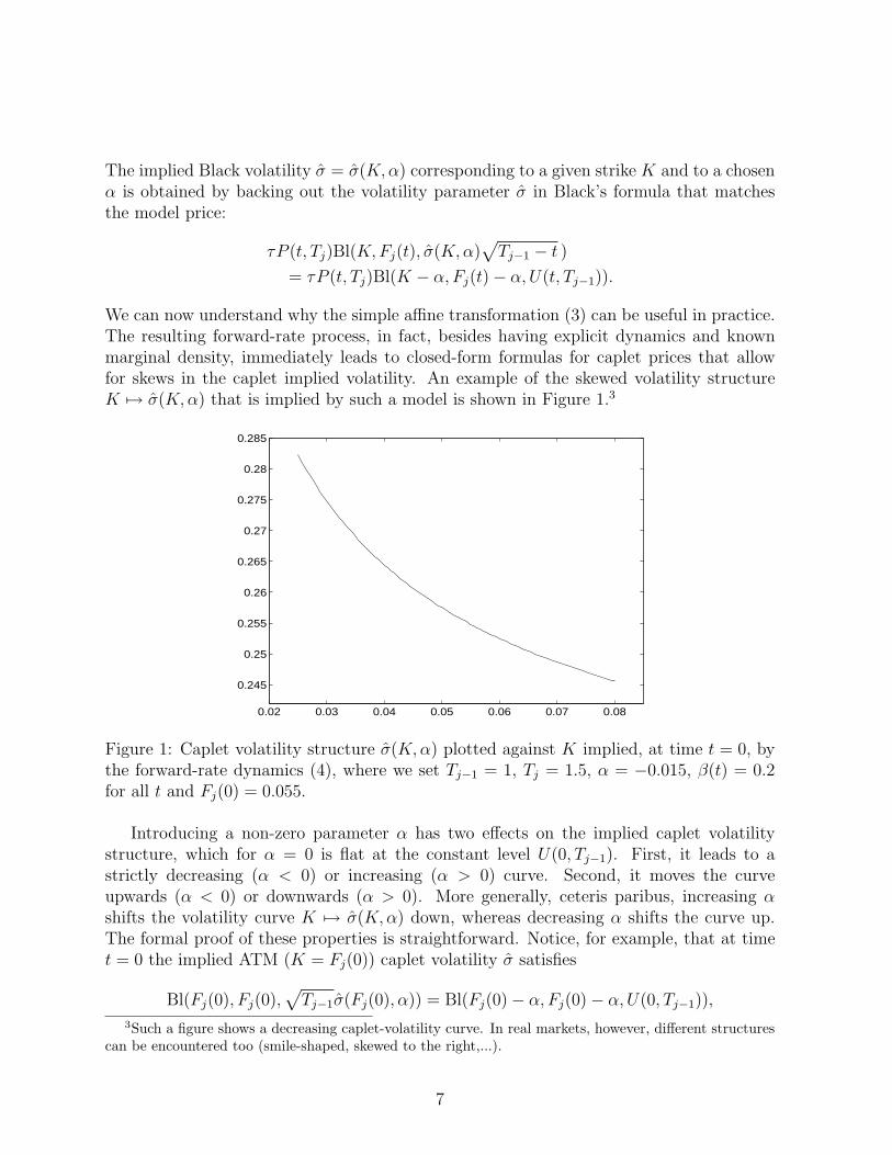
We can now understand why the simple affine transformation (3) can be useful in practice.The resulting forward-rate process, in fact, besides having explicit dynamics and knownmarginal density, immediately leads to closed-form formulas for caplet prices that allowfor skews in the caplet implied volatility. An example of the skewed volatility structureK 7→ σ(K, α) that is implied by such a model is shown in Figure 1.3

0.02 0.03 0.04 0.05 0.06 0.07 0.08

0.245

0.25

0.255

0.26

0.265

0.27

0.275

0.28

0.285

Figure 1: Caplet volatility structure σ(K,α) plotted against K implied, at time t = 0, bythe forward-rate dynamics (4), where we set Tj−1 = 1, Tj = 1.5, α = −0.015, β(t) = 0.2for all t and Fj(0) = 0.055.

Introducing a non-zero parameter α has two effects on the implied caplet volatilitystructure, which for α = 0 is flat at the constant level U(0, Tj−1). First, it leads to astrictly decreasing (α < 0) or increasing (α > 0) curve. Second, it moves the curveupwards (α < 0) or downwards (α > 0). More generally, ceteris paribus, increasing αshifts the volatility curve K 7→ σ(K,α) down, whereas decreasing α shifts the curve up.The formal proof of these properties is straightforward. Notice, for example, that at timet = 0 the implied ATM (K = Fj(0)) caplet volatility σ satisfies

Bl(Fj(0), Fj(0),√

Tj−1σ(Fj(0), α)) = Bl(Fj(0)− α, Fj(0)− α, U(0, Tj−1)),3Such a figure shows a decreasing caplet-volatility curve. In real markets, however, different structures

can be encountered too (smile-shaped, skewed to the right,...).

7

which reads

(Fj(0)− α)[

2Φ(

12U(0, Tj−1)

)

− 1]

= Fj(0)[

2Φ(

12

√

Tj−1σ(Fj(0), α))

− 1]

.

When increasing α the left hand side of this equation decreases, thus decreasing the σ inthe right-hand side that is needed to match the decreased left-hand side. Moreover, whendifferentiating (8) with respect to α we obtain a quantity that is always negative.

Shifting a lognormal diffusion can then help in recovering skewed volatility structures.However, such structures are often too rigid, and highly negative slopes are impossible torecover. Moreover, the best fitting of market data is often achieved for decreasing impliedvolatility curves, which correspond to negative values of the α parameter, and hence to asupport of the forward-rate density containing negative values. Even though the probabilityof negative rates may be negligible in practice, many people regard this drawback as anundesirable feature.

The next models we illustrate may offer the properties and flexibility required for asatisfactory fitting of market data.

3.2 The Constant Elasticity of Variance Model

Another classical model leading to skews in the implied caplet-volatility structure is theCEV model of Cox (1975) and Cox and Ross (1976). Recently, Andersen and Andreasen(2000) applied the CEV dynamics as a model of the evolution of forward LIBOR rates.

Andersen and Andreasen start with a general forward-LIBOR dynamics of the followingtype, under measure Qj,

dFj(t) = φ(Fj(t))σj(t) dWt,

where φ is a general function. Andersen and Andreasen suggest as a particularly tractablecase in this family the CEV model, where

φ(Fj(t)) = [Fj(t)]γ,

with 0 < γ < 1. Notice that the “border” cases γ = 0 and γ = 1 would lead respectivelyto a normal and a lognormal dynamics.

The model then reads

dFj(t) = σj(t)[Fj(t)]γ dWt, Fj = 0 absorbing boundary when 0 < γ < 1/2, (9)

where we set W = Zjj , a one-dimensional Brownian motion under the Tj forward measure.

For 0 < γ < 1/2 equation (9) does not have a unique solution unless we specify aboundary condition at Fj = 0. This is why we take Fj = 0 as an absorbing boundary forthe above SDE when 0 < γ < 1/2.4

4Andersen and Andreasen (2000) also extend their treatment to the case γ > 1, while noticing thatthis can lead to explosion when leaving the Tj-forward measure (under which the process has null drift).

8

Time dependence of σj can be dealt with through a deterministic time change. Indeed,by first setting

v(τ, T ) =∫ T

τσj(s)2ds

and then˜W (v(0, t)) :=

∫ t

0σj(s)dW (s),

we obtain a Brownian motion ˜W with time parameter v. We substitute this time changein equation (9) by setting fj(v(t)) := Fj(t) and obtain

dfj(v) = fj(v)γd˜W (v), fj = 0 absorbing boundary when 0 < γ < 1/2. (10)

This is a process that can be easily transformed into a Bessel process via a change ofvariable. Straightforward manipulations lead then to the transition density function of f .By also remembering our time change, we can finally go back to the transition densityfor the continuous part of our original forward-rate dynamics. The continuous part of thedensity function of Fj(T ) conditional on Fj(t), t < T ≤ Tj−1, is then given by

pFj(T )|Fj(t)(x) = 2(1− γ)k1/(2−2γ)(uw1−4γ)1/(4−4γ)e−u−wI1/(2−2γ)(2√

uw),

k =1

2v(t, T )(1− γ)2 ,

u = k[Fj(t)]2(1−γ),

w = kx2(1−γ),

(11)

with Iq denoting the modified Bessel function of the first kind of order q. Moreover,denoting by g(y, z) = e−zzy−1

Γ(y) the gamma density function and by G(y, x) =∫ +∞

x g(y, z)dzthe complementary gamma distribution, the probability that Fj(T ) = 0 conditional on

Fj(t) is G(

12(1−γ) , u

)

.A major advantage of the model (9) is its analytical tractability, allowing for the above

transition density function. This transition density can be useful, for example, in MonteCarlo simulations. From knowledge of the density follows also the possibility to price simpleclaims. In particular, the following explicit formula for a caplet price can be derived:

Cpl(t, Tj−1, Tj, τ,K) = τP (t, Tj)

[

Fj(t)+∞∑

n=0

g(n + 1, u) G(

cn, kK2(1−γ))

−K+∞∑

n=0

g (cn, u) G(

n + 1, kK2(1−γ))]

,

(12)

where k and u are defined as in (11) and

cn := n + 1 +1

2(1− γ).

9

This price can be expressed also in terms of the non-central chi-squared distribution func-tion we have encountered in the CIR model. Recall that we denote by χ2(x; r, ρ) thecumulative distribution function for a non-central chi-squared distribution with r degreesof freedom and non-centrality parameter ρ, computed at point x. Then the above pricecan be rewritten as

Cpl(t, Tj−1, Tj, τ,K)=τP (t, Tj)[

Fj(t)(

1− χ2(

2K1−γ;1

1− γ+2, 2u

)

)

−Kχ2(

2u;1

1− γ, 2kK1−γ

)

]

.(13)

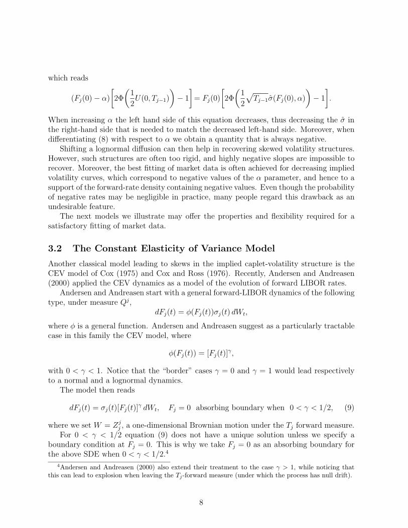
As hinted at above, the caplet price (12) leads to skews in the implied volatility structure.An example of the structure that can be implied is shown in Figure 2. As previously

0.03 0.04 0.05 0.06 0.07 0.080.17

0.18

0.19

0.2

0.21

0.22

0.23

Figure 2: Caplet volatility structure implied by (12) at time t = 0, where we set Tj−1 = 1,Tj = 1.5, σj(t) = 1.5 for all t, γ = 0.5 and Fj(0) = 0.055.

done in the case of a geometric Brownian motion, an extension of the above model can beproposed based on displacing the CEV process (9) and defining accordingly the forward-rate dynamics. The introduction of the extra parameter determining the density shiftingmay improve the calibration to market data.

Finally, there is the possibly annoying feature of absorption in F = 0. While thisdoes not necessarily constitute a problem for caplet pricing, it can be an undesirablefeature from an empirical point of view. Also, it is not clear whether there could be someproblems when pricing more exotic structures. As a remedy to this absorption problem,Andersen and Andreasen (2000) propose a “Limited” CEV (LCEV) process, where insteadof φ(F ) = F γ they set

φ(F ) = F min(εγ−1, F γ−1) ,

10

where ε is a small positive real number. This function collapses the CEV diffusion coefficientF γ to a (lognormal) level-proportional diffusion coefficient Fεγ−1 when F is small enough tomake little difference (smaller than ε itself). Andersen and Andreasen (2000) compare theLCEV and CEV models as far as cap prices are concerned and conclude that the differencesare small and tend to vanish when ε → 0. They also investigate, to some extent, the speedof convergence. A Crank-Nicholson scheme is used to compute cap prices within the LCEVmodel. As for the CEV model itself, Andersen and Andreasen allow for γ > 1 also in theLCEV case, with the difference that then ε has to be taken very large.

As far as the calibration of the CEV model to swaptions is concerned, approximatedswaption prices based on “freezing the drift” and “collapsing all measures” are also derived.See Andersen and Andreasen (2000) for the details.

4 A Class of Analytically-Tractable Models

We now propose a class of analytically tractable models that are flexible enough to recovera large variety of market volatility structures.

Let the dynamics of the forward rate Fj under the forward measure Qj be expressedby

dFj(t) = σ(t, Fj(t))Fj(t) dWt, (14)

where σ is a well-behaved deterministic function.The function σ, which is usually termed local volatility in the financial literature, must

be chosen so as to grant a unique strong solution to the SDE (14). In particular, we assumethat σ(·, ·) satisfies, for a suitable positive constant L, the linear-growth condition

σ2(t, y)y2 ≤ L(1 + y2) uniformly in t, (15)

which basically ensures existence of a strong solution.Let us then consider N diffusion processes with dynamics given by

dGi(t) = vi(t, Gi(t)) dWt, i = 1, . . . , N, Gi(0) = Fj(0) , (16)

with common initial value Fj(0), and where vi(t, y)’s are real functions satisfying regularityconditions to ensure existence and uniqueness of the solution to the SDE (16). In particularwe assume that, for suitable positive constants Li’s, the following linear-growth conditionshold:

v2i (t, y) ≤ Li(1 + y2) uniformly in t, i = 1, . . . , N. (17)

For each t, we denote by pit(·) the density function of Gi(t), i.e., pi

t(y) = d(QT{Gi(t) ≤y})/dy, where, in particular, pi

0 is the δ-Dirac function centered in Gi(0).The problem we want to address is the derivation of the local volatility σ(t, St) such

that the Qj-density of Fj(t) satisfies, for each time t,

pt(y) :=ddy

QT{Fj(t) ≤ y} =N

∑

i=1

λiddy

QT{Gi(t) ≤ y} =N

∑

i=1

λipit(y), (18)

11

where the λi’s are strictly positive constants such that∑N

i=1 λi = 1. Indeed, pt(·) is aproper QT -density function since, by definition,

∫ +∞

0ypt(y)dy =

N∑

i=1

λi

∫ +∞

0ypi

t(y)dy =N

∑

i=1

λiGi(0) = Fj(0).

Remark 4.1. Notice that in the last calculation we were able to recover the proper Qj-expectation thanks to our assumption that all processes (16) share the same null drift.However, the role of the processes Gi is merely instrumental, and there is no need toassume their drift to be of that form if not for simplifying calculations. In particular,what matters in obtaining the right expectation as in the last formula above is the marginaldistribution pi.

As already noticed by several authors,5 the above problem is essentially the reverse tothat of finding the marginal density function of the solution of an SDE when the coefficientsare known. In particular, σ(t, Fj(t)) can be found by solving the Fokker-Planck equation

∂∂t

pt(y) =12

∂2

∂y2

(

σ2(t, y)y2pt(y))

, (19)

given that each density pit(y) satisfies itself the Fokker-Planck equation

∂∂t

pit(y) =

12

∂2

∂y2

(

v2i (t, y)pi

t(y))

. (20)

Applying the definition (18) and the linearity of the derivative operator, (19) can be writtenas

N∑

i=1

λi∂∂t

pit(y) =

N∑

i=1

λi

[

− ∂∂y

(

µypit(y)

)

]

+N

∑

i=1

λi

[

12

∂2

∂y2

(

σ2(t, y)y2pit(y)

)

]

,

which by substituting from (20) becomes

N∑

i=1

λi

[

12

∂2

∂y2

(

v2i (t, y)pi

t(y))

]

=N

∑

i=1

λi

[

12

∂2

∂y2

(

σ2(t, y)y2pit(y)

)

]

.

Using again linearity of the second order derivative operator, we obtain

∂2

∂y2

[

N∑

i=1

λiv2i (t, y)pi

t(y)

]

=∂2

∂y2

[

σ2(t, y)y2N

∑

i=1

λipit(y)

]

.

If we look at this last equation as to a second order differential equation for σ(t, ·), we findeasily its general solution

σ2(t, y)y2N

∑

i=1

λipit(y) =

N∑

i=1

λiv2i (t, y)pi

t(y) + Aty + Bt, (21)

5See for instance Dupire (1997).

12

with A and B suitable real functions of time. The regularity conditions (17) and (15) implythat the LHS of the equation has zero limit for y →∞. As a consequence, the RHS musthave a zero limit as well. This holds if and only if At = Bt = 0, for each t. We thereforeobtain that the expression for σ(t, y) that is consistent with the marginal density (18) andwith the regularity constraint (15) is, for (t, y) > (0, 0),

σ(t, y) =

√

∑Ni=1 λiv2

i (t, y)pit(y)

∑Ni=1 λiy2pi

t(y). (22)

Indeed, notice that by setting

Λi(t, y) :=λipi

t(y)∑N

i=1 λipit(y)

(23)

for each i = 1, . . . , N and (t, y) > (0, 0), we can write

σ2(t, y) =N

∑

i=1

Λi(t, y)v2

i (t, y)y2 , (24)

so that the square of the volatility σ can be written as a (stochastic) convex combinationof the squared volatilities of the basic processes (16). In fact, for each (t, y), Λi(t, y) ≥ 0for each i and

∑Ni=1 Λi(t, y) = 1. Moreover, by (17) and setting L := maxi=1,...,N Li, the

condition (15) is fulfilled since

σ2(t, y)y2 =N

∑

i=1

Λi(t, y)v2i (t, y) ≤

N∑

i=1

Λi(t, y)Li(1 + y2) ≤ L(1 + y2).

The function σ may be then extended to the semi-axes {(t, 0) : t > 0} and {(0, y) : y > 0}according to the specific choice of the basic densities pi

t(·).Formula (22) leads to the following SDE for the forward rate under measure Qj:

dFj(t) =

√

∑Ni=1 λiv2

i (t, Fj(t))pit(Fj(t))

∑Ni=1 λiFj(t)2pi

t(Fj(t))Fj(t) dWt. (25)

This SDE, however, must be regarded as defining some candidate dynamics that leads tothe marginal density (18). Indeed, if σ is bounded, then the SDE is well defined, but theconditions we have imposed so far are not sufficient to grant the uniqueness of the strongsolution, so that a verification must be done on a case-by-case basis.

Let us now assume that the SDE (25) has a unique strong solution. We will see later ona fundamental case where this assumption holds. Then, remembering the definition (18), itis straightforward to derive the model caplet prices in terms of the caplet prices associated

13

to the basic models (16). Indeed, let us consider a caplet with strike K associated to thegiven forward rate. Then, the caplet price at the initial time t = 0 is given by

Cpl(0, Tj−1, Tj, τ, K) = τP (0, Tj)Ej {

[Fj(T )−K)]+}

= τP (0, Tj)N

∑

i=1

λi

∫ +∞

0[y −K]+pi

Tj(y)dy

=N

∑

i=1

λiCpli(0, Tj−1, Tj, τ,K),

(26)

where Cpli(0, Tj−1, Tj, τ, K) denotes the caplet price, with unit notional amount, associatedwith (16).

We can now justify our assumption that the forward rate marginal density be given bythe mixture of known basic densities. When proposing alternative dynamics, it is usuallyquite problematic to come up with analytical formulas for caplets. Here, instead, suchproblem can be avoided since the beginning if we use analytically-tractable densities pi.6

Moreover, the absence of bounds on the parameter N implies that a virtually unlimitednumber of parameters can be introduced in the dynamics so as to be used for a bettercalibration to market data.

A last remark concerns the classical economic interpretation of a mixture of densities.We can indeed view Fj as a process whose density at time t coincides with the basic densitypi

t with probability λi.

5 A Mixture-of-Lognormals Model

Let us now consider the particular case where the densities pit’s are all lognormal. Precisely,

we assume that, for each i,vi(t, y) = σi(t)y, (27)

where all σi’s are deterministic and continuous functions of time that are bounded fromabove and below by (strictly) positive constants.

The marginal density of Gi(t), for each time t, is then lognormal and given by

pit(y) =

1yVi(t)

√2π

exp

{

− 12V 2

i (t)

[

lny

Fj(0)+ 1

2V2i (t)

]2}

,

Vi(t) :=

√

∫ t

0σ2

i (u)du.

(28)

Brigo and Mercurio (2001a) proved the following.6Note that, due to the linearity of the derivative operator, the same convex combination applies to all

Greeks.

14

Proposition 5.1. Let us assume there exists an ε > 0 such that σi(t) = σ0 > 0, for eacht in [0, ε] and i = 1, . . . , N . Then, if we set

ν(t, y) :=

√

√

√

√

√

√

√

∑Ni=1 λiσ2

i (t)1

Vi(t)exp

{

− 12V 2

i (t)

[

ln yFj(0) + 1

2V2i (t)

]2}

∑Ni=1 λi

1Vi(t)

exp{

− 12V 2

i (t)

[

ln yFj(0) + 1

2V2i (t)

]2} , (29)

for (t, y) > (0, 0) and ν(t, y) = σ0 for (t, y) = (0, Fj(0)), the SDE

dFj(t) = ν(t, Fj(t))Fj(t) dWt (30)

has a unique strong solution whose marginal density is given by the mixture of lognormals

pt(y) =N

∑

i=1

λi1

yVi(t)√

2πexp

{

− 12V 2

i (t)

[

lny

Fj(0)+ 1

2V2i (t)

]2}

(31)

The above proposition provides us with the analytical expression for the diffusion coef-ficient in the SDE (14) such that the resulting equation has a unique strong solution whosemarginal density is given by (31).

The square of the local volatility ν(t, y) can be viewed as a weighted average of thesquared basic volatilities σ2

1(t), . . . , σ2N(t), where the weights are all functions of the log-

normal marginal densities (28). That is, for each i = 1, . . . , N and (t, y) > (0, 0), we canwrite

ν2(t, y) =N

∑

i=1

Λi(t, y)σ2i (t),

Λi(t, y) :=λipi

t(y)∑N

i=1 λipit(y)

.

As a consequence, for each t > 0 and y > 0, the function ν is bounded from below andabove by (strictly) positive constants. In fact

σ∗ ≤ ν(t, y) ≤ σ∗ for each t, y > 0, (32)

where

σ∗ := inft≥0

{

mini=1,...,N

σi(t)}

> 0,

σ∗ := supt≥0

{

maxi=1,...,N

σi(t)}

< +∞.

Remark 5.2. The function ν(t, y) can be extended by continuity to the semi-axes {(0, y) :y > 0} and {(t, 0) : t ≥ 0} by setting ν(0, y) = σ0 and ν(t, 0) = ν∗(t), where ν∗(t) := σi∗(t)

15

and i∗ = i∗(t) is such that Vi∗(t) = maxi=1,...,N Vi(t). In particular, ν(0, 0) = σ0. Indeed,for every y > 0 and every t ≥ 0,

limt→0

ν(t, y) = σ0,

limy→0

ν(t, y) = ν∗(t).

At time t = 0, the pricing of caplets under our forward-rate dynamics (30) is quitestraightforward. Indeed,

P (0, Tj)Ej{[Fj(Tj−1)−K]+} = P (0, Tj)∫ +∞

0(y −K)+pTj−1(y)dy

= P (0, Tj)N

∑

i=1

λi

∫ +∞

0(y −K)+pi

Tj−1(y)dy

so that, the caplet price Cpl(0, Tj−1, Tj, τ, K) associated with our dynamics (30) is simplygiven by

Cpl(0, Tj−1, Tj, τ, N, K) = τP (0, Tj)N

∑

i=1

λiBl(K, Fj(0), Vi(Tj−1)). (33)

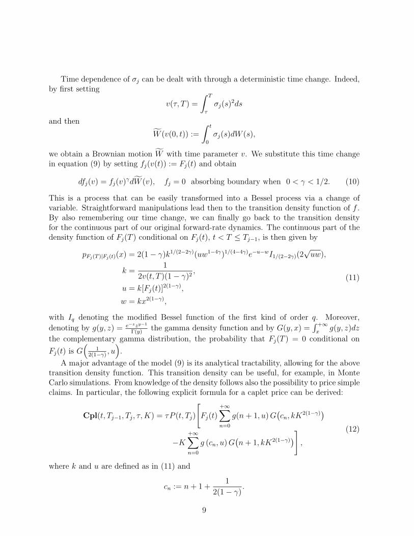
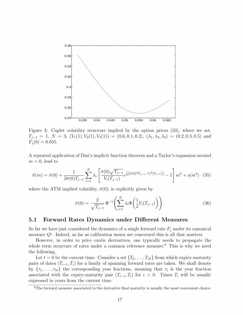
The caplet price (33) leads to smiles in the implied volatility structure. An exampleof the shape that can be reproduced is shown in Figure 3.7 Observe that the impliedvolatility curve has a minimum exactly at a strike equal to the initial forward rate Fj(0).This property, which is formally proven in Brigo and Mercurio (2000a), makes the modelsuitable for recovering smile-shaped volatility surfaces. In fact, also skewed shapes can beretrieved, but with zero slope at the ATM level.

Given the above analytical tractability, we can easily derive an explicit approximationfor the caplet implied volatility as a function of the caplet strike price. More precisely,define the moneyness m as the logarithm of the ratio between the forward rate and thestrike, i.e.,

m := lnFj(0)

K.

The implied volatility σ(m) for the moneyness m is implicitly defined by equating theBlack caplet price in σ(m) to the price implied by our model according to

[

Φ

(

m + 12 σ(m)2Tj−1

σ(m)√

Tj−1

)

− e−mΦ

(

m− 12 σ(m)2Tj−1

σ(m)√

Tj−1

)]

=N

∑

i=1

λi

[

Φ(

m + 12V

2i (Tj−1)

Vi(Tj−1)

)

− e−mΦ(

m− 12V

2i (Tj−1)

Vi(Tj−1)

)]

.

(34)

7In such a figure, we consider directly the values of the Vi’s. Notice that one can easily find some σi’ssatisfying our technical assumptions that are consistent with the chosen Vi’s.

16

0.035 0.04 0.045 0.05 0.055 0.06 0.0650.24

0.26

0.28

0.3

0.32

0.34

0.36

0.38

Figure 3: Caplet volatility structure implied by the option prices (33), where we set,Tj−1 = 1, N = 3, (V1(1), V2(1), V3(1)) = (0.6, 0.1, 0.2), (λ1, λ2, λ3) = (0.2, 0.3, 0.5) andFj(0) = 0.055.

A repeated application of Dini’s implicit function theorem and a Taylor’s expansion aroundm = 0, lead to

σ(m) = σ(0) +1

2σ(0)Tj−1

N∑

i=1

λi

[

σ(0)√

Tj−1

Vi(Tj−1)e

18(σ(0)2Tj−1−V 2

i (Tj−1)) − 1

]

m2 + o(m3) (35)

where the ATM implied volatility, σ(0), is explicitly given by

σ(0) =2

√

Tj−1Φ−1

(

N∑

i=1

λiΦ(

12Vi(Tj−1)

)

)

. (36)

5.1 Forward Rates Dynamics under Different Measures

So far we have just considered the dynamics of a single forward rate Fj under its canonicalmeasure Qj. Indeed, as far as calibration issues are concerned this is all that matters.

However, in order to price exotic derivatives, one typically needs to propagate thewhole term structure of rates under a common reference measure.8 This is why we needthe following.

Let t = 0 be the current time. Consider a set {T0, . . . , TM} from which expiry-maturitypairs of dates (Ti−1, Ti) for a family of spanning forward rates are taken. We shall denoteby {τ1, . . . , τM} the corresponding year fractions, meaning that τi is the year fractionassociated with the expiry-maturity pair (Ti−1, Ti) for i > 0. Times Ti will be usuallyexpressed in years from the current time.

8The forward measure associated to the derivative final maturity is usually the most convenient choice.

17

Proposition 5.1 applies to any forward rate, provided one consider different coefficientsfor different rates. Precisely, assume σi,j’s are deterministic and continuous functions oftime that are bounded from above and below by (strictly) positive constants, and thatthere exists an ε > 0 such that σi,j(t) = σ0

j > 0, for each t in [0, ε] and i = 1, . . . , N . Thendefine

Vi,j(t) :=

√

∫ t

0σ2

i,j(u)du

νj(t, y) :=

√

√

√

√

√

√

√

∑Ni=1 λi,j σ2

i,j(t)1

Vi,j(t)exp

{

− 12V 2

i,j(t)

[

ln yFj(0) + 1

2V2i,j(t)

]2}

∑Ni=1 λi,j

1Vi,j(t)

exp{

− 12V 2

i,j(t)

[

ln yFj(0) + 1

2V2i,j(t)

]2} ,

with λi,j > 0, for each i, j, and∑N

i=1 λi,j = 1 for each j.

Proposition 5.3. The dynamics of Fj = F (·; Tj−1, Tj) under the forward measure Qi inthe three cases i < j, i = j and i > j are, respectively,

i < j, t ≤ Ti :

dFj(t) = νj(t, Fj(t))Fj(t)j

∑

k=i+1

ρj,k τk νk(t, Fk(t)) Fk(t)1 + τkFk(t)

dt + νj(t, Fj(t))Fj(t) dW ij (t),

i = j, t ≤ Tj−1 :dFj(t) = νj(t, Fj(t))Fj(t) dW i

j (t),

i > j, t ≤ Tj−1 :

dFj(t) = −νj(t, Fj(t))Fj(t)i

∑

k=j+1

ρj,k τk νk(t, Fk(t)) Fk(t)1 + τkFk(t)

dt + νj(t, Fj(t))Fj(t) dW ij (t),

where W i = (W i1, . . . , W

iM) is an M-dimensional Brownian motion under Qi, with instan-

taneous correlation matrix (ρj,k), meaning that dW ij (t) dW i

k(t) = ρj,k dt.Moreover, all of the above equations admit a unique strong solution.

Proof. The proof is a direct consequence of Proposition 6.3.1. in Brigo and Mercurio (2001)and of the fact that all volatility coefficients νj’s are bounded.

Remark 5.4 (Swaptions pricing). In order to analytically price swaptions the classical“freezing-the-drift” technique9 can be employed for deriving analytical approximations of

9We refer to Brigo and Mercurio (2001) for an exhaustive explanation and justification of this method-ology.

18

implied swaption volatilities. For instance, in the case i < j, the above forward ratedynamics can be substituted by

dFj(t) = νj(t, Fj(0))Fj(t)j

∑

k=i+1

ρj,k τk νk(t, Fk(0)) Fk(t)1 + τkFk(t)

dt + νj(t, Fj(0))Fj(t) dW ij (t).

6 Shifting the Lognormal-Mixture Dynamics

Brigo and Mercurio (2000, 2001c) proposed a simple way to generalize the dynamics (30).With the main target consisting of retrieving a larger variety of volatility structures, thebasic lognormal-mixture model was combined with the displaced-diffusion technique byassuming that the forward-rate process Fj is given by

Fj(t) = α + Fj(t), (37)

where α is a real constant and Fj evolves according to the basic “lognormal mixture” dy-namics (30). It is easy to prove that this is actually the most general affine transformationfor which the forward-rate process is still a martingale under its canonical measure.

Dropping the index j where is redundant, so as to come back to the initial notation ofSection 5, the analytical expression for the marginal density of such a process is given bythe shifted mixture of lognormals

pt(y) =N

∑

i=1

λi1

(y − α)Vi(t)√

2πexp

{

− 12V 2

i (t)

[

lny − α

Fj(0)− α+ 1

2V2i (t)

]2}

,

with y > α.By Ito’s formula, we obtain that the forward rate process evolves according to

dFj(t) = ν(t, Fj(t)− α) (Fj(t)− α) dWt. (38)

This model for the forward rate process preserves the analytical tractability of the originalprocess Fj. Indeed,

P (0, Tj)Ej {

[Fj(Tj−1)−K]+}

= P (0, Tj)Ej{

[

F (Tj−1)− (K − α)]+

}

,

so that, for α < K, the caplet price Cpl(0, Tj−1, Tj, τ, K) associated with (37) is simplygiven by

Cpl(t, Tj−1, Tj, τ,K) = τP (t, Tj)N

∑

i=1

λiBl(K − α, Fj(0)− α, Vi(Tj−1)). (39)

19

Moreover, the caplet implied volatility (as a function of m) can be approximated as follows:

σ(m) = σ(0) + σ′(0)m +12σ′′(0)m2 + o(m2)

σ′(0) = α

√

2πTj−1

e18 σ(0)2Tj−1

Fj(0)

(

−N

∑

i=1

λiΦ(

12Vi(Tj−1)

)

+12

)

σ′′(0) =Fj(0)

Fj(0)− α

N∑

i=1

λie

18 (σ(0)2Tj−1−Vi(Tj−1)2)

Vi(Tj−1)√

Tj−1−

4− σ(0)2σ′(0)2T 2j−1

4σ(0)Tj−1,

where the ATM implied volatility, σ(0), is explicitly given by

σ(0) =2

Fj(0)√

Tj−1Φ−1

(

(Fj(0)− α)N

∑

i=1

λiΦ(

12Vi(Tj−1)

)

+α2

)

. (40)

For α = 0 the process Fj obviously coincides with Fj while preserving the correct zero drift.The introduction of the new parameter α has the effect that, decreasing α, the variance ofthe asset price at each time increases while maintaining the correct expectation. Indeed:

E(Fj(t)) = Fj(0),

Var(Fj(t)) = (Fj(0)− α)2

(

N∑

i=1

λieV 2i (t) − 1

)

.

As for the model (3), the parameter α affects the shape of the implied volatility curve intwo ways. First, it concurs to determine the level of such curve in that changing α leadsto an almost parallel shift of the curve itself. Second, it moves the strike with minimumvolatility. Precisely, if α > 0 (< 0) the minimum is attained for strikes lower (higher) thanthe ATM’s. When varying all parameters, the parameter α can be used to add asymmetryaround the ATM volatility without shifting the curve.

Finally, as far as the calibration of the above models to swaptions is concerned, onceagain approximated swaption prices similar to Rebonato’s formula in the FLM and based on“freezing the drift” and “collapsing all measures” approaches can be attempted, althoughresults need to be checked numerically in a sufficiently rich number of situations.

7 Two Further Alternative Dynamics

We now consider two further examples in the class of Section 4. The resulting processes,though slightly more involved than (30), have the major advantage of being more flexibleas far as the implied caplet volatility curves are concerned.

20

7.1 A Lognormal-Mixture with Different Means

In the first example we consider, the densities pit’s are still lognormal, but their means

are now assumed to be different. Precisely, we assume that the instrumental processes Gi

evolve, under Qj, according to

dGi(t) = µi(t)Gi(t)dt + σi(t)Gi(t) dWt, i = 1, . . . , N, Gi(0) = Fj(0) ,

where σi’s satisfy the conditions of Section 5, and µi’s are deterministic functions of time.The density of Gi at time t is thus given by

pit(y) =

1yVi(t)

√2π

exp

{

− 12V 2

i (t)

[

lny

Fj(0)−Mi(t) + 1

2V2i (t)

]2}

,

Mi(t) :=∫ t

0µi(u)du,

with Vi defined as before. The functions µi’s can not be defined arbitrarily, but must bechosen so that

N∑

i=1

λieMi(t) = 1, ∀t > 0.

This is because pt(y) =∑N

i=1 λipit(y) must have a constant mean equal to Fj(0).

As in Section 4, we look for a diffusion coefficient ψ(·, ·) such that

dFj(t) = ψ(t, Fj(t))Fj(t) dWt (41)

has a solution with marginal density pt(y) =∑N

i=1 λipit(y). As before, we then use the

Fokker-Planck equations for processes Fj and Gi’s to find that

ψ(t, y)2 := ν(t, y) +2∑N

i=1 λiµi(t)∫ +∞

y xpit(x)dx

y2∑N

i=1 λipit(y)

, (42)

with ν defined as in (29), namely

ν(t, y)2 =∑N

i=1 λiσi(t)2pit(y)

∑Mi=1 λipi

t(y),

where the new pit’s are to be used.

Remark 7.1. The integrals in the numerator of the second term in the RHS of (42)are quantities proportional the Black-Scholes prices of asset or nothing options for theinstrumental processes Gi.

21

The coefficient ψ is not necessarily well defined, since the second term in the RHS of(42) can become negative for some choices of the basic parameters. However, the functionν is bounded from below by a strictly positive constant, so that it is possible to deriveconditions under which positivity of ψ(t, y)2 is granted (at least for y in a compact set).Under these conditions is then easy to prove that the diffusion coefficient ψ(t, Fj(t))Fj(t)has linear growth and does not explode in finite time, i.e. that the resulting SDE admitsa unique strong solution.

The pricing of caplets, under dynamics (41), is again quite straightforward. Indeed,the caplet price Cpl(0, Tj−1, Tj, τ,K) is simply given by

Cpl(0, Tj−1, Tj, τ,K) = τP (0, Tj)N

∑

i=1

λieMi(Tj−1)Bl(

K e−Mi(Tj−1), Fj(0), Vi(Tj−1))

. (43)

Also this price leads to smiles in the implied volatility structure. However, the non-zerodrifts in the Gi-dynamics allows us to reproduce steeper and more skewed curves than inthe zero-drifts case, with minimums that can be shifted far away from the ATM level.

7.2 The Case of Hyperbolic-Sine Processes

The second case we consider lies in the class of dynamics (25). We in fact assume that thebasic processes Gi evolve, under Qj, according to a hyperbolic-sine process, i.e.10

Gi(t) = βi(t) sinh [αi(Wt − Li)] , i = 1, . . . , N, Gi(0) = Fj(0) , (44)

where αi’s are positive constant, Li’s are negative constants, and βi’s are chosen so as torender the Gi’s martingales, namely

βi(t) =Fj(0) e−

12α2

i t

sinh(−αiLi).

The SDE followed by each Gi is thus given by

dGi(t) = αi

√

β2i (t) + G2

i (t) dWt, i = 1, . . . , N.

Looking at this SDE’s diffusion coefficient we immediately notice that it is roughly de-terministic for small values of Gi(t), whereas it is roughly proportional to Gi(t) for largevalues of Gi(t). Therefore in the former case, the dynamics are approximately of Gaussiantype, whereas in the latter they are approximately of lognormal type. For further detailson such a process we refer to Carr et al. (1999).11

The hyperbolic-sine process (44) shares all the analytical tractability of the classicalgeometric Brownian motion. This is intuitive, since (44) is basically the difference of twogeometric Brownian motions (with perfectly negatively correlated logarithms).

10We remind that sinh(x) = ex−e−x

2 , and that sinh−1(x) = ln(x +√

1 + x2).11Carr et al. (1999) actually consider a process where negative values are absorbed into zero. Their

process is slightly more complicated, but not lose in analytical tractability.

22

The cumulative distribution function of process Gi at each time t is easily derived asfollows:

Qj{Gi(t) ≤ y} = Qj{

Wt ≤ Li +1αi

sinh−1(

yβi(t)

)}

= Φ(

Li√t

+1

αi√

tsinh−1

(

yβi(t)

))

,

so that the time-t marginal density of Gi is

pit(y) =

1

αi√

2πt√

β2i (t) + y2

exp

[

− 12t

(

Li +1αi

sinh−1(

yβi(t)

))2]

. (45)

Moreover, through a straightforward integration, we obtain the associated caplet price as

Cpl(0, Tj−1, Tj, τ,K) = τP (0, Tj)[

Fj(0)2 sinh(−αiLi)

(

e−αiLiΦ(

y(Tj−1) + αi

√

Tj−1

)

− eαiLiΦ(

y(Tj−1)− αi

√

Tj−1

)

)

−KΦ(

y(Tj−1))

]

,(46)

where we set, for a general t,

y(t) := − Li√t− 1

αi√

tsinh−1

(

Kβi(t)

)

. (47)

The pricing function (46) leads to steeply decreasing patterns in the implied volatilitycurve. Therefore, we can hope that a mixture of densities (45) leads to steeper impliedvolatility skews than in the lognormal-mixture model. Indeed, this turns out to be thecase.

The results in Section 4, and equation (25) in particular, immediately yield the followingSDE for the forward rate under measure Qj:

dFj(t) = χ(t, Fj(t)) dWt

χ(t, y) :=

√

√

√

√

√

√

√

∑Ni=1 λiαi exp

[

− 12t

(

Li + 1αi

sinh−1(

yβi(t)

))2]

∑Ni=1 λi

1αi

√β2

i (t)+y2exp

[

− 12t

(

Li + 1αi

sinh−1(

yβi(t)

))2] .

(48)

This equation, however, must be handled with due care. Indeed, the function χ is discon-tinuous in (0, Fj(0)), so that the existence and uniqueness of a solution remains an openissue.

A possible solution is given by introducing time-dependent coefficients, as we did inSection 5, and imposing suitable restrictions on them.

23

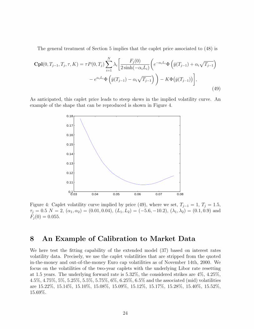
The general treatment of Section 5 implies that the caplet price associated to (48) is

Cpl(0, Tj−1, Tj, τ,K) = τP (0, Tj)N

∑

i=1

λi

[

Fj(0)2 sinh(−αiLi)

(

e−αiLiΦ(

y(Tj−1) + αi

√

Tj−1

)

− eαiLiΦ(

y(Tj−1)− αi

√

Tj−1

)

)

−KΦ(

y(Tj−1))

]

,

(49)

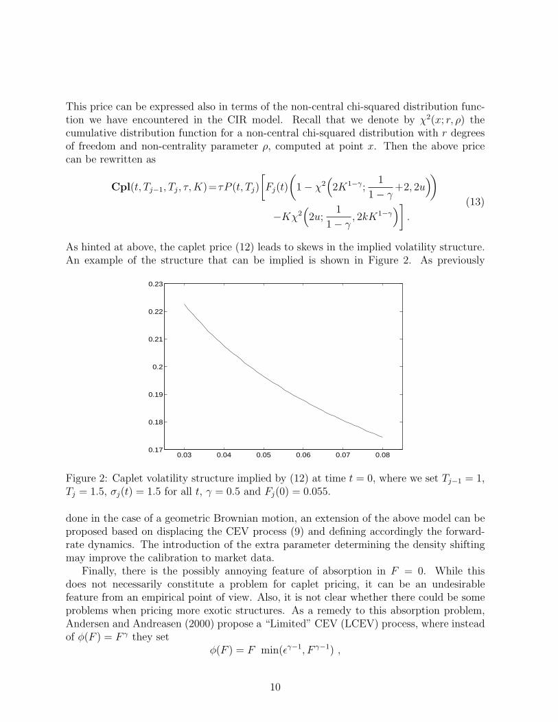
As anticipated, this caplet price leads to steep skews in the implied volatility curve. Anexample of the shape that can be reproduced is shown in Figure 4.

0.03 0.04 0.05 0.06 0.07 0.080.1

0.11

0.12

0.13

0.14

0.15

0.16

0.17

0.18

Figure 4: Caplet volatility curve implied by price (49), where we set, Tj−1 = 1, Tj = 1.5,τj = 0.5 N = 2, (α1, α2) = (0.01, 0.04), (L1, L2) = (−5.6,−10.2), (λ1, λ2) = (0.1, 0.9) andFj(0) = 0.055.

8 An Example of Calibration to Market Data

We here test the fitting capability of the extended model (37) based on interest ratesvolatility data. Precisely, we use the caplet volatilities that are stripped from the quotedin-the-money and out-of-the-money Euro cap volatilities as of November 14th, 2000. Wefocus on the volatilities of the two-year caplets with the underlying Libor rate resettingat 1.5 years. The underlying forward rate is 5.32%, the considered strikes are 4%, 4.25%,4.5%, 4.75%, 5%, 5.25%, 5.5%, 5.75%, 6%, 6.25%, 6.5% and the associated (mid) volatilitiesare 15.22%, 15.14%, 15.10%, 15.08%, 15.09%, 15.12%, 15.17%, 15.28%, 15.40%, 15.52%,15.69%.

24

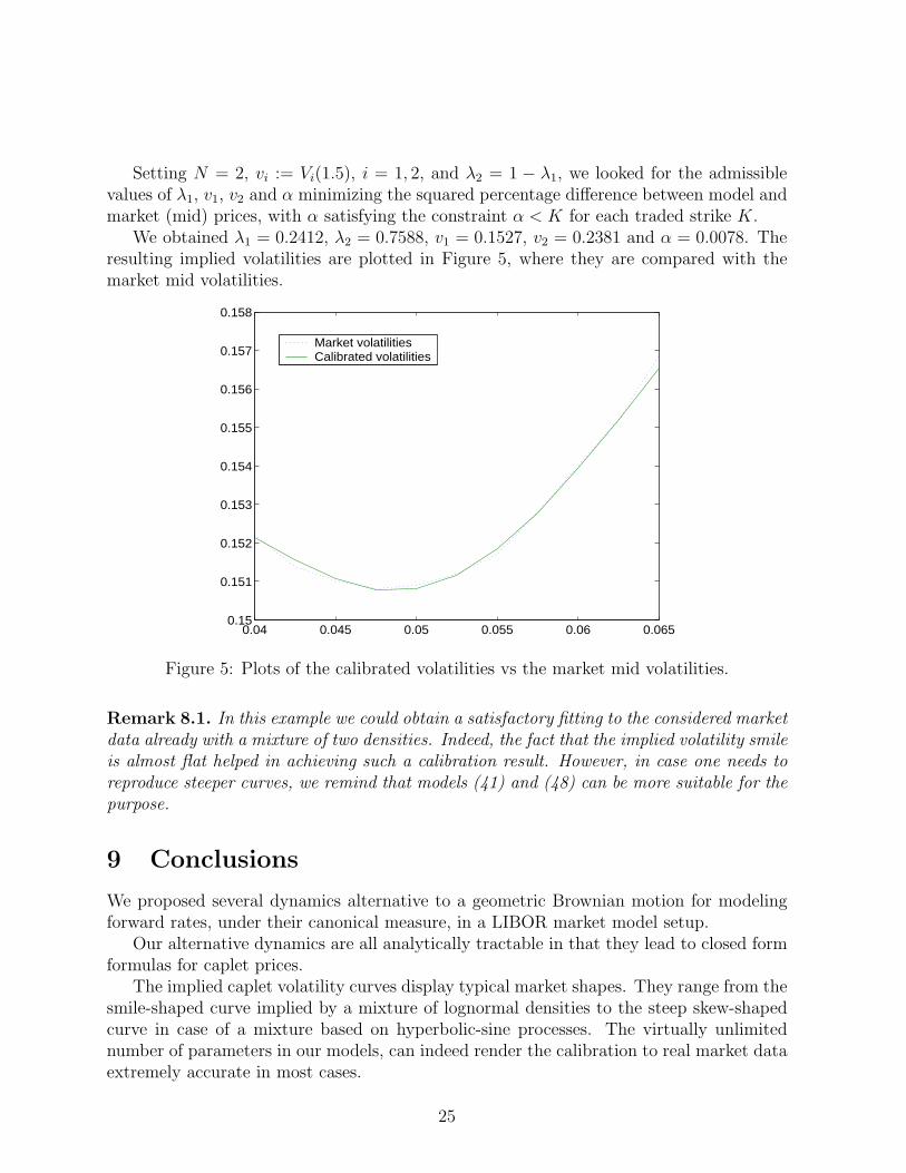
Setting N = 2, vi := Vi(1.5), i = 1, 2, and λ2 = 1 − λ1, we looked for the admissiblevalues of λ1, v1, v2 and α minimizing the squared percentage difference between model andmarket (mid) prices, with α satisfying the constraint α < K for each traded strike K.

We obtained λ1 = 0.2412, λ2 = 0.7588, v1 = 0.1527, v2 = 0.2381 and α = 0.0078. Theresulting implied volatilities are plotted in Figure 5, where they are compared with themarket mid volatilities.

0.04 0.045 0.05 0.055 0.06 0.0650.15

0.151

0.152

0.153

0.154

0.155

0.156

0.157

0.158

Market volatilities Calibrated volatilities

Figure 5: Plots of the calibrated volatilities vs the market mid volatilities.

Remark 8.1. In this example we could obtain a satisfactory fitting to the considered marketdata already with a mixture of two densities. Indeed, the fact that the implied volatility smileis almost flat helped in achieving such a calibration result. However, in case one needs toreproduce steeper curves, we remind that models (41) and (48) can be more suitable for thepurpose.

9 Conclusions

We proposed several dynamics alternative to a geometric Brownian motion for modelingforward rates, under their canonical measure, in a LIBOR market model setup.

Our alternative dynamics are all analytically tractable in that they lead to closed formformulas for caplet prices.

The implied caplet volatility curves display typical market shapes. They range from thesmile-shaped curve implied by a mixture of lognormal densities to the steep skew-shapedcurve in case of a mixture based on hyperbolic-sine processes. The virtually unlimitednumber of parameters in our models, can indeed render the calibration to real market dataextremely accurate in most cases.

25

Two are the main issues needing further investigation: i) the analysis of the evolutionof the caplet volatility curves implied in the future by our models; ii) the stability in timeof the model parameters. These are, indeed, the by-now classical problematic features onehas to face when dealing with local-volatility models like ours.

References

[1] Andersen, L., and Andreasen, J. (2000). Volatility Skews and Extensions of theLIBOR Market Model. Applied Mathematical Finance 7, 1-32.

[2] Avellaneda, M., Friedman, C., Holmes, R. and Samperi D. (1997) Calibrating Volatil-ity Surfaces via Relative-Entropy Minimization. Preprint. Courant Institute of Math-ematical Sciences. New York University.

[3] Black, F. and Scholes, M. (1973) The Pricing of Options and Corporate Liabilities.Journal of Political Economy 81, 637-659.

[4] Bhupinder, B. (1998) Implied Risk-Neutral Probability Density Functions from Op-tion Prices: A Central Bank Perspective. In Forecasting Volatility in the FinancialMarkets, 137-167. Edited by Knight, J., and Satchell, S. Butterworth Heinemann.Oxford.

[5] Brace, A., Goldys, B., Klebaner, F., and Womersley, R. (2001). Market Model ofStochastic Implied Volatility with application to the BGM Model. Working PaperS01-1, Department of Statistics, University of New South Wales, Sydney.

[6] Breeden, D.T. and Litzenberger, R.H. (1978) Prices of State-Contingent Claims Im-plicit in Option Prices. Journal of Business 51, 621-651.

[7] Brigo, D., and Mercurio, F. (2000). A mixed-up smile. Risk September, 123-126.

[8] Brigo, D., Mercurio, F. (2001a) Displaced and Mixture Diffusions for Analytically-Tractable Smile Models. In Mathematical Finance - Bachelier Congress 2000, Geman,H., Madan, D.B., Pliska, S.R., Vorst, A.C.F., eds. Springer Finance, Springer, BerlinHeidelberg New York.

[9] Brigo, D., Mercurio, F. (2001b) Lognormal-Mixture Dynamics and Calibration toMarket Volatility Smiles, International Journal of Theoretical & Applied Finance,forthcoming.

[10] Brigo, D., Mercurio, F. (2001c) Interest Rate Models: Theory and Practice. SpringerFinance. Springer.

[11] Britten-Jones, M. and Neuberger, A. (1999) Option Prices, Implied Price Processesand Stochastic Volatility. Preprint. London Business School.

26

[12] Carr, P., Tari, M. and Zariphopoulou T. (1999) Closed Form Option Valuation withSmiles. Preprint. NationsBanc Montgomery Securities.

[13] Cox, J. (1975) Notes on Option Pricing I: Constant Elasticity of Variance Diffusions.Working paper. Stanford University.

[14] Cox, J. and Ross S. (1976) The Valuation of Options for Alternative StochasticProcesses. Journal of Financial Economics 3, 145-166.

[15] Derman, E. and Kani, I. (1994) Riding on a Smile. Risk February, 32-39.

[16] Derman, E. and Kani, I. (1998) Stochastic Implied Trees: Arbitrage Pricing withStochastic Term and Strike Structure of Volatility. International Journal of Theoret-ical and Applied Finance 1, 61-110.

[17] Dupire, B. (1994) Pricing with a Smile. Risk January, 18-20.

[18] Dupire, B. (1997) Pricing and Hedging with Smiles. Mathematics of Derivative Se-curities, edited by M.A.H. Dempster and S.R. Pliska, Cambridge University Press,Cambridge, 103-111.

[19] Guo, C. (1998) Option Pricing with Heterogeneous Expectations. The FinancialReview 33, 81-92.

[20] Heston, S. (1993) A Closed Form Solution for Options with Stochastic Volatility withApplications to Bond and Currency Options. Review of Financial Studies 6, 327-343.

[21] Hull, J. and White, A. (1987) The Pricing of Options on Assets with StochasticVolatilities. Journal of Financial and Quantitative Analysis 3, 281-300.

[22] Jackwerth, J.C. and Rubinstein, M. (1996) Recovering Probability Distributions fromOption Prices. Journal of Finance 51, 1611-1631.

[23] Ledoit, O. and Santa-Clara, P. (1998) Relative Pricing of Options with StochasticVolatility. Working paper, Anderson Graduate School of Management, University ofCalifornia, Los Angeles.

[24] Melick, W.R., and Thomas, C.P. (1997) Recovering an Asset’s Implied PDF fromOption Prices: An Application to Crude Oil During the Gulf Crisis. Journal ofFinancial and Quantitative Analysis 32, 91-115.

[25] Musiela, M. and Rutkowski, M. (1998) Martingale Methods in Financial Modelling.Springer. Berlin.

[26] Prigent, J.L, Renault O. and Scaillet O. (2000) An Autoregressive Conditional Bi-nomial Option Pricing Model. Preprint. Universite de Cergy.

[27] Rebonato, R. (2001). The stochastic volatility Libor market model. Risk October, - .

27

[28] Ritchey, R.J. (1990) Call Option Valuation for Discrete Normal Mixtures. Journalof Financial Research 13, 285-296.

[29] Rubinstein, M. (1994) Implied Binomial Trees. Journal of Finance 49, 771-818.

[30] Shimko, D. (1993) Bounds of Probability. Risk April, 33-37.

[31] Schonbucher, P. (1999) A Market Model of Stochastic Implied Volatility. Philosoph-ical Transactions of the Royal Society, Series A, Vol. 357, No. 1758, pp. 2071-2092.

[32] Tompkins, R.G. (2000a) Stock Index Futures Markets: Stochastic Volatility Modelsand Smiles. Preprint. Department of Finance. Vienna University of Technology.

[33] Tompkins, R.G. (2000b) Fixed Income Futures Markets: Stochastic Volatility Modelsand Smiles. Preprint. Department of Finance. Vienna University of Technology.

28