PRICING EQUITY DERIVATIVES SUBJECT TO …users.iems.northwestern.edu/~linetsky/default.pdfPRICING...

Mathematical Finance, Vol. 16, No. 2 (April 2006), 255–282

PRICING EQUITY DERIVATIVES SUBJECT TO BANKRUPTCY

VADIM LINETSKY

Northwestern University, Evanston, Illinois

We solve in closed form a parsimonious extension of the Black–Scholes–Mertonmodel with bankruptcy where the hazard rate of bankruptcy is a negative power ofthe stock price. Combining a scale change and a measure change, the model dynamicsis reduced to a linear stochastic differential equation whose solution is a diffusionprocess that plays a central role in the pricing of Asian options. The solution is inthe form of a spectral expansion associated with the diffusion infinitesimal generator.The latter is closely related to the Schrodinger operator with Morse potential. Pricingformulas for both corporate bonds and stock options are obtained in closed form. Termcredit spreads on corporate bonds and implied volatility skews of stock options areclosely linked in this model, with parameters of the hazard rate specification controllingboth the shape of the term structure of credit spreads and the slope of the impliedvolatility skew. Our analytical formulas are easy to implement and should prove usefulto researchers and practitioners in corporate debt and equity derivatives markets.

KEY WORDS: bankruptcy, credit risk, hazard rate, credit spread, stock options, implied volatilityskew, Asian options, Brownian exponential functionals, Schrodinger operator with Morse potential,spectral expansions

1. INTRODUCTION

In the celebrated Black–Scholes–Merton model the firm’s stock price is assumed tofollow geometric Brownian motion (GBM)—a diffusion process with constant volatil-ity and infinite life time. On one hand, this assumption precludes bankruptcy. To thecontrary, modeling bankruptcy and credit spreads is at the center of the literature oncorporate bonds (see recent monographs Bielecki and Rutkowski [2002], Duffie andSingleton [2003], Lando [2004], and Schonbucher [2003], for a summary of the credit riskliterature). On the other hand, the GBM assumption contradicts the accumulated empir-ical evidence on implied volatility skews exhibited by stock options prices. Modeling theimplied volatility skew is at the center of the equity derivatives literature (e.g., Rubinstein1994; Jackwerth and Rubinstein 1996).

Until recently, the literature on stock options and the literature on corporate bondsdeveloped more or less independently. Recently, the two strands of literature have mergedon the topic of modeling convertible bonds, as convertible bonds are corporate bondswith embedded stock option features. In the reduced-form framework, one specifies thehazard rate of bankruptcy as a decreasing function of the underlying stock price, h = h(S).The bankruptcy event is modeled as the first jump time of a doubly stochastic Poisson

This research was supported by the U.S. National Science Foundation under Grant DMI-0200429.Manuscript received October 2004; final revision received January 2005.Address correspondence to V. Linetsky, Department of Industrial Engineering and Management Sciences,

McCormick School of Engineering and Applied Sciences, Northwestern University, 2145 Sheridan Road,Evanston, IL 60208; e-mail: [email protected].

C© 2006 The Author. Journal compilation C© 2006 Blackwell Publishing Inc., 350 Main St., Malden, MA 02148,USA, and 9600 Garsington Road, Oxford OX4 2DQ, UK.

255

256 V. LINETSKY

process with intensity h, and the term structure of credit spreads is determined from thespecification of the intensity and the parameters of the underlying stock price process.The negative power intensity provides a particularly parsimonious specification:

h(S) = αS−p(1.1)

for some p > 0 and α > 0. This specification was recently employed in Andersen andBuffum (2003), Ayache, Forsyth, and Vetzal (2003), Davis and Lischka (2002), Duffieand Singleton (2003, p. 216), Muromachi (1999), and Takahashi, Kobayashi, and Naka-gawa (2001) in the context of modeling convertible bonds. Muromachi (1999) empiricallyestimated the value of the power parameter p to be in the range between 1.2 and 2 forJapanese bonds rated BB+ and below. In these references the convertible bond pricewas determined numerically by finite-difference or lattice methods. The negative powerintensity model has become popular among practitioners for convertible bond modeling.While the main focus of these references is on pricing convertible bonds, Andersen andBuffum (2003) showed that this class of models exhibits implied volatility skews in stockoption prices, with the parameters of the hazard rate specification controlling the slope ofthe skew, thus establishing a link between implied volatility skews and credit spreads (seealso Hull, Nelken, and White [2004] for the linkage between credit spreads and impliedvolatility skews in Merton’s structural model).

In the present paper we solve the negative power intensity model in closed form both forcorporate bonds and European-style stock options. We start in Section 2 by introducingbankruptcy into the GBM model by killing the process at the rate h = h(S ), where h isa decreasing function of the underlying stock price. To insure that the discounted stockprice is a martingale under equivalent martingale measure (EMM), the hazard rate h(S)needs to be added to the drift rate of the process (e.g., Davis and Lischka 2002). We thendiscuss the pricing of equity derivatives in this diffusion-with-killing model and show that,by Girsanov’s theorem, the risky discount factor with the hazard rate can be removedfrom the valuation relationships at the expense of modifying the drift of the underlyingdiffusion, thus reducing the problem to the study of the diffusion process (2.3) withoutkilling. In Section 3 we adopt the negative power specification (1.1) and show that thevaluation problem further reduces to the problem of computing expectations with respectto the distribution of the diffusion process X (ν) solving the linear stochastic differentialequation (SDE) (3.4). This process has recently been studied in the context of pricingarithmetic Asian options (see Donati-Martin, Ghomrasni, and Yor [2001] and Linetsky[2004a] and references therein). Fortunately, the spectral representation of its transitiondensity is available in closed form (Proposition 3.3), and we are able to compute all thenecessary integrals in closed form and obtain closed-form expressions for both corpo-rate bonds (Proposition 3.4) and European-style stock options (Proposition 3.5). Theseclosed-form expressions are in the form of spectral expansions (for recent applicationsof the spectral expansion method to derivatives pricing see Lewis [1998], Gorovoi andLinetsky [2004], Linetsky [2004a–2004d] and references therein). In Section 4 our analyti-cal solutions are employed to develop an economic analysis of the model. In particular, westudy possible shapes and asymptotics of the term structure of credit spreads and impliedvolatility skews in the negative power intensity model, and explore the link between creditspreads and implied volatility skews. Section 5 concludes the paper. Appendix A presentsadditional mathematical details on the process X (ν) and its density p(ν) and their con-nections with several classical mathematical objects (Schrodinger operator with Morsepotential and Maass Laplacian on the hyperbolic plane). Appendix B discusses the closerelationship of the process X (ν) to the pricing of Asian options (Geman and Yor 1992,1993; Donati-Martin, Ghomrasni, and Yor 2001; Linetsky 2004a). Appendix C collects

PRICING EQUITY DERIVATIVES SUBJECT TO BANKRUPTCY 257

the necessary facts about special functions appearing in the pricing formulas. Appendix Dcontains proofs.

2. EQUITY DERIVATIVES SUBJECT TO BANKRUPTCYIN THE INTENSITY-BASED FRAMEWORK

2.1. The Stock Price Model

Let (�,G, P) be a probability space supporting a standard Brownian motion {Bt, t ≥0} and an exponential random variable e ∼ Exp(1) with unit parameter independent ofB. Let h = h(x) be a nonnegative function on R+ satisfying the following assumptions.

ASSUMPTION 2.1. We assume that h is C1(0, ∞), strictly decreasing, and has the fol-lowing limits:

limx→0

h(x) = +∞, limx→∞ h(x) = 0.

We take an EMM P as given and model the pre-bankruptcy underlying stock pricedynamics under the EMM as a diffusion process {St, t ≥ 0} solving the SDE

dSt = (r − q + h(St))St dt + σ St dBt, S0 = S > 0,(2.1)

where r > 0, q > 0, and σ > 0 are the risk-free interest rate, dividend yield, and pre-bankruptcy stock price volatility, respectively. Under Assumption 2.1, the SDE (2.1)has a unique strong nonexploding solution. This solution is a diffusion process on (0,∞) with both zero and infinity inaccessible boundaries. To see this, consider a process{Xt := σ−1ln St, t ≥ 0},

dXt = (μ + σ−1h(eσ Xt )) dt + dBt, X0 = σ−1 ln S, μ = (r − q − σ 2/2)/σ.

Under Assumption 2.1, this SDE has a unique strong nonexploding solution. Stronguniqueness up to the explosion time is insured by h ∈ C1 (e.g., Ikeda and Watanabe1981). Nonexplosion can be checked by applying Feller’s test for explosions (e.g., Karlinand Taylor 1981, p. 234).

We model the random time of bankruptcy τ as the first time when the process∫ t0 h(Su) du is greater or equal to the random level e (equivalently, as the first jump time of

a doubly stochastic Poisson process (Cox process) with intensity (hazard rate) ht = h(St)):

τ = inf{

t ≥ 0 :∫ t

0h(Su) du ≥ e

}.

At the time of bankruptcy τ , the stock price jumps to the bankruptcy state, �, where itremains forever (� is a cemetery state in the terminology of Markov processes; e.g., Revuzand Yor 1999). We assume that equity holders do not receive any recovery in the event ofbankruptcy and their equity position becomes worthless. In other words, we model thestock price subject to bankruptcy as a diffusion process {S�

t , t ≥ 0} with the extended statespace E� = (0, ∞) ∪ {�}, diffusion coefficient a(x) = σx, drift b(x) = (r − q + h(x))x,and killing rate h(x). In our notation, {St, t ≥ 0} is the pre-bankruptcy stock priceprocess (2.1), while {S�

t , t ≥ 0} is the stock price process subject to bankruptcy, so thatS�

t = St for t < τ and S�t = � for all t ≥ τ .

The addition of the hazard rate in the drift rate in the pre-bankruptcy dynamics (2.1)compensates for the bankruptcy jump to insure that the total expected rate of return to the

258 V. LINETSKY

stockholder is equal to the risk-free rate in the risk-neutral economy and the discountedgain process is a martingale under EMM (e.g., Davis and Lischka 2002). Our assumptionsabout the hazard rate are intuitive. As the stock price declines towards zero, the hazardrate increases to infinity. As the stock price increases, the hazard rate declines to zero,making the stock price process asymptotically GBM.

To keep track of how information is revealed over time, following Elliot et al. (2000),we introduce a bankruptcy jump indicator process {Dt, t ≥ 0}, Dt = 1{t≥τ }, denote byD = {Dt, t ≥ 0} a filtration generated by D, by F = {Ft, t ≥ 0} a filtration generated bythe Brownian motion B, and by G = {Gt, t ≥ 0}, Gt = Ft ∨ Dt, an enlarged filtration. Thedefaultable stock process S� is adapted to the enlarged filtration G.

If we identify the cemetery state � = 0, then we can write the process for the stockprice subject to bankruptcy in the form

dS�t = S�

t−((r − q) dt + σ dBt − dMt),

where

Mt = Dt −∫ t∧τ

0h(Su) du,

is a martingale (compensated bankruptcy jump process).

2.2. Equity Derivatives

A European-style equity derivative with maturity (expiration) at time T > 0 is definedby its payoff F : E� → R+,

F(S�

T

) = F(S�

T

)1{S�

T �=�} + R1{S�T =�},

where F(S�T )1{S�

T �=�} is the payoff at maturity, given no bankruptcy prior to T , and R =F(�) ≥ 0 is the recovery payment at maturity in the event of bankruptcy. The valuationof the two parts of the payoff is standard in the reduced-form intensity-based credit riskmodeling framework1

e−rTE[F

(S�

T

)1{S�

T �=�}] = e−rTE

[F(ST)1{τ>T}

]= e−rTE

[F(ST)E

[1{τ>T}

∣∣FT]] = e−rTE

[e− ∫ T

0 h(St) dt F(ST)],

and

e−rTE[R1{S�

T =�}] = e−rTE

[R1{τ≤T}

] = e−rT R(1 − E

[1{τ>T }

])= e−rT R

(1 − E

[E

[1{τ>T }

∣∣FT]]) = e−rT R

(1 − E

[e− ∫ T

0 h(St) dt]),where {Ft, t ≥ 0} is the filtration generated by the Brownian motion B, and we used thefact that

E[1{τ>T }

∣∣FT] = e− ∫ T

0 h(St) dt.

These valuations reduce to computing expectations of the form

Vψ (S, T) = e−rTE[e− ∫ T

0 h(St) dtψ(ST)].

1 See Duffie, Schroder, and Skiadas (1996), Duffie and Singleton (1999), Jarrow and Turnbull (1995),Jarrow, Lando, and Turnbull (1997), and Madan and Unal (1998), as well as recent monographs Bieleckiand Rutkowski (2002), Duffie and Singleton (2003), Lando (2004), and Schonbucher (2003). For the partialdifferential equation (PDE) approach to the pricing of equity derivatives with the hazard rate dependent onthe underlying stock price, see Carr and Javaheri (2005).


This can be interpreted as pricing a claim with payoff ψ(ST ) at T > 0 in a fictitiouseconomy with the risk-free interest rate process rt = r + h(St), stock price process (2.1),and no bankruptcy. The discount factor with h can be removed by changing the probabilitymeasure.

PROPOSITION 2.1.

Vψ (S, T ) = e−rTE[e− ∫ T

0 h(St) dtψ(ST)] = e−qT S E

[S−1

T ψ(ST)],(2.2)

where E is the expectation with respect to the probability measure P under which Bt :=Bt − σ t is a standard Brownian motion and

dS t = (r − q + σ 2 + h(St)

)St dt + σ St dBt, S0 = S > 0.(2.3)

Proof . From equation (2.1) we have

St = Se(r−q)t+∫ t0 h(Su ) du+σ Bt− 1

2 σ 2t, t ≥ 0,

and hence

e−rTE[e− ∫ T

0 h(St) dtψ(ST)]

= e−qT SE[eσ BT− 1

2 σ 2T S−1T ψ(ST)

].

Application of Girsanov’s theorem completes the proof. �

In particular, for fixed T > 0, we will be interested in a zero-coupon bond with unitface value and constant recovery payment 0 ≤ R < 1 at maturity, a call option with strikeK > 0 with the payoff (ST − K)+ at expiration and no recovery if the firm goes bankrupt,and a put option with strike K > 0 with the payoff (K − ST )+ if τ >T and recoverypayment R = K at expiration in the event of bankruptcy τ ≤ T (note that we decomposethe put payoff into two parts: (K − ST )+1{τ>T} + K1{τ≤T}). Using Proposition 2.1, thepricing formulas for the bond, call, and put take the form

BR(S, T ) = e−rT R + (1 − R)e−qT S E[S−1

T

],(2.4a)

CK (S, T ) = e−qT S E[(

1 − K S−1T

)+],(2.4b)

PK (S, T ) = e−qT S E[(

K S−1T − 1

)+] + K(e−rT − e−qT S E

[S−1

T

]),(2.4c)

respectively. In particular, the put–call parity is satisfied by

CK (S, T ) − PK (S, T ) = e−qT S − e−rT K .(2.5)

One notes that the put pricing formula (2.4c) consists of two parts: the present value ofthe put payoff given no bankruptcy,

e−qT S E[(

KS−1T − 1

)+],(2.6)

and the present value of the recovery in the event of bankruptcy,

K(e−rT − B(S, T )),(2.7)

where

B(S, T ) = e−rTP(τ > T) = e−qT S E[S−1

T

](2.8)

260 V. LINETSKY

is the price of the T-maturity zero-coupon bond with unit face value and zero recovery(the subscript 0 in B0(S, T) will be dropped for zero-recovery bonds) and P(τ > T) is the(risk-neutral) probability of surviving beyond time T (survival probability). The recoverypart of the put option is termed a bankruptcy claim by Lewis (1998) in the context ofMerton’s model with constant dividend rate, where the bankruptcy occurs when the stockprice process hits zero.

3. ANALYTICAL SOLUTION FOR THE NEGATIVEPOWER INTENSITY MODEL

3.1. The Negative Power Intensity Model

A parsimonious specification for the hazard rate satisfying Assumption 2.1 is

h(S) = αS−p, α > 0, p > 0.(3.1)

This specification was employed in Andersen and Buffum (2003), Ayache, Forsyth, andVetzal (2003), Davis and Lischka (2002), Duffie and Singleton (2003, p. 216), Muromachi(1999), and Takahashi, Kobayashi, and Nakagawa (2001) in the context of modelingconvertible bonds. Muromachi (1999) estimated the value of the power parameter p tobe in the range between 1.2 and 2 for Japanese bonds rated BB+ and below. In thesereferences the convertible bond price was determined numerically by finite-difference orlattice methods. The negative power intensity model (3.1) has become popular amongpractitioners for convertible bond modeling. In the present paper we solve the modelboth for corporate bonds and European-style stock options in closed form.

We are interested in calculating expectations (2.2) under the process (2.3) with h givenby Ito’s (3.1). First, introduce a new process {Zt := βSp

t , t ≥ 0}, where β = pσ 2/(4α).From Ito’s formula, it solves the linear SDE

dZt = (aZt + b) dt + cZt dBt, Z0 = z = βSp,(3.2)

with parameters

a = p(r − q + (p + 1)σ 2/2) ∈ R, b = p2σ 2/4 > 0, c = pσ > 0.

This linear SDE has a well-known solution (e.g., Karatzas and Shreve 1992, pp. 360–361)

Zt = e(a−c2/2)t+cBt

(z + b

∫ t

0e−(a−c2/2)u−cBu du

), t ≥ 0.

Using the Brownian scaling property cBt(law)= 2Bc2t/4, we can effect a time change so that

Zt = X (ν)τ (t), τ (t) = p2σ 2t/4,

where X (ν) is the standardized process:

X (ν)t = e2(νt+Bt)

(z +

∫ t

0e−2(νu+Bu )du

), t ≥ 0, with ν = 2

pσ 2

(r − q + σ 2

2

),

(3.3)

solving the standardized linear SDE2

dX (ν)t = (

2(ν + 1)X (ν)t + 1

)dt + 2X (ν)

t dBt, X (ν)0 = x = z = βSp.(3.4)

2 We note that this SDE was derived by Shiryaev (1961) in the context of quickest detection problems (seePeskir 2004).


Thus, the valuation equation (2.2) is reduced to

Vψ (S, T ) = e−qT SE(ν)x

[χψ

(X(ν)

τ

)], x = βSp, β = pσ 2/(4α), τ = p2σ 2T/4,

(3.5)

where the expectation E(ν)x is with respect to the law of the process X (ν) started at x

and

χψ (y) := (y/β)−1/pψ((y/β)1/p).(3.6)

3.2. The Process X (ν), Its Resolvent Kernel, and Transition Density

In this section we review the properties of the diffusion process X (ν).

PROPOSITION 3.1. The boundary at zero is entrance for all ν ∈ R. The boundary atinfinity is natural for all ν ∈ R. For ν > 0 it is attracting and the process is transient. Forν ≤ 0 it is nonattracting. For ν < 0 the process is positive recurrent and possesses a stationarydistribution with the density

π (x) = 2ν

�(−ν)xν−1e− 1

2x .(3.7)

Proof . The scale and speed densities of X (ν) are (see, e.g., Borodin and Salminen2002, p. 17, for scale and speed densities of one-dimensional diffusions)

s(x) = x−ν−1e1

2x , m(x) = 12

xν−1e− 12x .(3.8)

The nature of the boundaries at zero and infinity are established by applying Feller’sboundary classification criteria based on the behavior of the scale and speed densi-ties (Borodin and Salminen 2002, pp. 14–15). For ν < 0 the speed measure is finite,∫ ∞

0 m(x) dx < ∞, and hence, the process is positive recurrent with the stationary densitygiven by the normalized speed density (Borodin and Salminen 2002, pp. 20–21). �

Let p(ν)(t; x, y) be the transition density of X (ν) and, for s > 0, G(ν)s (x, y) its Laplace

transform in time (also called resolvent kernel or Green’s function, e.g., Borodin andSalminen 2002, pp. 19–20)3

G(ν)s (x, y) =

∫ ∞

0e−st p(ν)(t; x, y) dt.(3.9)

PROPOSITION 3.2. For x, y > 0, the resolvent kernel is given by (x ∧ y := min{x, y},x ∨ y := max{x, y}):

G(ν)s (x, y) = �

(μ(s) + ν

2

)(yx

) ν−12

e1

4x − 14y M 1−ν

2 ,μ(s)

(1

2(x ∨ y)

)W1−ν

2 ,μ(s)

(1

2(x ∧ y)

),

(3.10)

where

μ(s) = 12

√2s + ν2,(3.11)

3 Note that our Green’s function and transition density are defined with respect to the Lebesgue measure,while Borodin and Salminen’s are defined with respect to the speed measure and, thus, our Green’s functionand transition density differ from Borodin and Salminen’s by a factor of m(y).

262 V. LINETSKY

�(z) is the Gamma function, and Mκ,μ(z) and W κ,μ (z) are the Whittaker functions (C.2)and (C.3). For x = 0 and y > 0 the Green’s function reduces to

G(ν)s (0, y) = �

(μ(s) + ν

2

)(2y)

ν−12 e− 1

4y M 1−ν2 ,μ(s)

(1

2y

).

Proof . See Appendix D.

REMARK 3.1. This Green’s function was obtained by Donati-Martin, Ghomrasni, andYor (2001, Theorem 3.1) by solving the differential equation. The transition density isrecovered by inverting the Laplace transform. This produces the spectral representationfor the transition density (see McKean [1956] and Ito and McKean [1974, Section 4.11]for the spectral representation of the transition density of a one-dimensional diffusion,and Linetsky [2004b; 2006] and references therein for applications in finance).

PROPOSITION 3.3. For x, y > 0 and ν ∈ R, the transition density has the followingspectral representation

p(ν)(t; x, y) = 1{ν<0}π (y) + 1{ν<−2}[|ν|/2]∑n=1

e−2n(|ν|−n)t 2(|ν| − 2n)n!�(1 + |ν| − n)

e− 12y (2x)n(2y)n−1−|ν|

× L(|ν|−2n)n

(1

2x

)L(|ν|−2n)

n

(1

2y

)+ 1

2π2

∫ ∞

0e− (ν2+ρ2)t

2 e1

4x − 14y

(yx

) ν−12

× W1−ν2 ,

iρ2

(1

2x

)W1−ν

2 ,iρ2

(1

2y

)∣∣∣∣�(ν + iρ

2

)∣∣∣∣2

sinh(πρ)ρ dρ,

(3.12)

where L(α)n (x) are the generalized Laguerre polynomials, [x] denotes the integer part of x,

and 1{·} is the indicator. When x = 0, y > 0, and ν ∈ R,

p(ν)(t; 0, y) = 12π2

∫ ∞

0e− (ν2+ρ2)t

2 e− 14y (2y)

ν−12 W1−ν

2 ,iρ2

(1

2y

) ∣∣∣∣� (ν + iρ

2

)∣∣∣∣2

sinh(πρ)ρ dρ

+ 1{ν<0}π (y) + 1{ν<−2}[|ν|/2]∑n=1

e−2n(|ν|−n)t (−1)n2(|ν| − 2n)�(1 + |ν| − n)

× e− 12y (2y)n−1−|ν|L(|ν|−2n)

n

(1

2y

).


REMARK 3.2. The density in Proposition 3.3 has a long history and is closely relatedto a number of classical mathematical objects. For ν < 0 this density was first obtainedby Wong (1964, p. 271, equation (38)) in his studies of diffusions with stationary densitiesin the Pearson family. See Comtet, Monthus, and Yor (1998), Linetsky (2004a), andAppendix A and B for details. In Appendix D we provide a proof for all ν ∈ R.

REMARK 3.3. Because the boundary at zero is entrance, the process can be started atzero and G(ν)

s (0, y) and p(ν)(t; 0, y) exist. In the application to Asian options the process isstarted at zero (see Appendix B). In the present application to equity derivatives subjectto bankruptcy, the process is started at a positive value x = βSp > 0.


REMARK 3.4. For ν ≥ 0 the spectrum of the infinitesimal generator

G(ν) = 2x2 d 2

dx2 + (2(ν + 1) + 1)ddx

of X (ν) in the Hilbert space of functions square-integrable with the speed density m inequation (3.8) is purely continuous (the integral term in the spectral expansion (3.12)). Forν < 0 there is some nonempty discrete spectrum that contains at least the zero principaleigenvalue. The term in the spectral expansion (3.12) corresponding to the zero principaleigenvalue is the stationary density π (3.7). The spectral expansion for the transitiondensity can be obtained by directly inverting the Laplace transform of the resolvent kernel,using the Cauchy Residue Theorem. The resolvent kernel (3.10) needs to be considered inthe complex s-plane. The poles of the resolvent kernel (the poles of the Gamma functionin equation (3.10) for ν < 0) give the eigenvalues, and the integral along the branch cut{s = −ν2/2 − ρ2/2, ρ ∈ [0, ∞)} produces the continuous part of the spectral expansion.See Appendix D for this approach. Alternatively, the spectral expansion can be obtainedby employing the real-variable approach by first considering a truncated spectral problemon [0, b] for some b > 0 with the Dirichlet boundary condition at b and purely discretespectrum, and then passing to the limit b → ∞ (this approach is detailed in Linetsky2004a).

3.3. Pricing L2 Payoffs

We now apply the spectral representation to the valuation problem (3.5). Let H :=L2((0, ∞),m) be the Hilbert space of functions square-integrable with the speed density m

in equation (3.8) and endowed with the inner product

( f , g)m =∫ ∞

0f (x)g(x)m(x) dx.

For any ψ such that χψ ∈ H (χψ is defined in (3.6)), the valuation (3.5) has the spectralrepresentation

eqT S−1Vψ (S, T ) = 12π2

∫ ∞

0e− (ν2+ρ2)τ

2 Cψ (ρ)x1−ν

2 e1

4x

× W1−ν2 ,

iρ2

(1

2x

) ∣∣∣∣� (ν + iρ

2

)∣∣∣∣2

sinh(πρ)ρ dρ

+ 1{ν<0}cψ (0) + 1{ν<−2}[|ν|/2]∑n=1

cψ (n)e−2n(|ν|−n)τ

× 2(|ν| − 2n)n!�(1 + |ν| − n)

(2x)n L(|ν|−2n)n

(1

2x

),

(3.13)

where the expansion coefficients are given by

Cψ (ρ) =∫ ∞

0y

ν−12 e− 1

4y W1−ν2 ,

iρ2

(1

2y

)χψ (y) dy,(3.14)

cψ (0) =∫ ∞

0χψ (y)π (y) dy, cψ (n) =

∫ ∞

0(2y)n−|ν|−1 e− 1

2y L(|ν|−2n)n

(1

2y

)χψ (y) dy.

(3.15)

264 V. LINETSKY

For details of the spectral expansion approach to derivatives pricing, see Linetsky (2004b)and references therein.

3.4. Pricing Bonds

First consider the case ν < 2/p (from equation (3.3) this condition is equivalent tor − q − σ 2/2 < 0). Bond payoff ψbond(x) = 1 is such that χψ ∈ H, and the spectral rep-resentation (3.13) is applicable. Fortunately, in this case the integrals in equations (3.14)and (3.15) can be calculated in closed form.

The case ν ≥ 2/p (equivalently, r − q − σ 2/2 ≥ 0) is more involved. For the bondpayoff ψbond(x) = 1, χψ (x) = (x/β)−1/p /∈ H and, hence, the spectral representation(3.13) cannot be applied. The alternative is to first compute the Laplace transform

�(ν)s (x) :=

∫ ∞

0e−sτ E(ν)

x

[(X(ν)

τ /β)−1/p]

dτ =∫ ∞

0(y/β)−1/pG(ν)

s (x, y) dy(3.16)

with the kernel (3.10) and then do the Laplace inversion, choosing the contour of integra-tion in the Bromwich complex Laplace inversion formula to the right of any singularitiesof �

(ν)s (x) in the complex s-plane. In this case the function �

(ν)s (x) has an additional pole

in addition to the singularities inherited from the Green’s function G(ν)s (x, y), resulting

in an additional positive term in the pricing formula for ν > 2/p (this phenomenon fornon-L2 payoffs has been first discussed in Lewis 1998). The interpretation of this addi-tional term as the discounted probability of the firm asymptotically escaping to largestock price values and ultimately avoiding bankruptcy is provided in Section 4.

PROPOSITION 3.4. The pricing function (2.8) for the zero-coupon bond with unit facevalue and no recovery is given by

B(S, T ) = 1{ν>2/p}e−rT �(ν − 1/p)�(ν − 2/p)

U(

1p,

2p

− ν + 1,1

2x

)+ 1{ν<0}e−qT �(1/p − ν)

�(−ν)(2x)

1p

+ 1{ν<−2}e−qT[|ν|/2]∑n=1

e−2n(|ν|−n)τ (|ν| − 2n)�(−1/p)�(1/p + |ν| − n)�(1 + |ν| − n)�(1 − 1/p − n)

× (2x)1p +n L(|ν|−2n)

n

(1

2x

)+ e−qT

4π2�(1/p)

∫ ∞

0e− (ν2+ρ2)τ

2 (2x)1p + 1−ν

2 e1

4x

× W1−ν2 ,

iρ2

(1

2x

) ∣∣∣∣� (ν + iρ

2

)�

(1p

− ν + iρ2

)∣∣∣∣2

sinh(πρ)ρ dρ,

where U(a, b, z) is the second confluent hypergeometric function (see Appendix C ).


3.5. Pricing Options

The put payoff ψ(x) = (K − x)+ is such that χψ ∈ H for all ν ∈ R and, hence, thevaluation of the put payoff given no bankruptcy (2.6) follows from the spectral expansion(3.13). Fortunately, the integrals in the expressions for the expansion coefficients (3.14)and (3.15) can be computed in closed form. The recovery part (bankruptcy claim) value(2.7) follows from the bond valuation in Proposition 3.4.


PROPOSITION 3.5. Define k = βKp. The put pricing function (2.4c) is given by

PK (S, T ) = e−rT K − 1{ν>2/p}e−rT K�(ν − 1/p)�(ν − 2/p)

U(

1p,

2p

− ν + 1,1

2x

)− 1{ν<0}

e−qT S�(|ν|)

[�

(|ν|, 1

2k

)+ (2k)

1p γ

(1p

+ |ν|, 12k

)]

− 1{ν<−2}e−qT S[|ν|/2]∑n=1

pK (n)e−2n(|ν|−n)τ 2(|ν| − 2n)n!�(1 + |ν| − n)

(2x)n L(|ν|−2n)n

(1

2x

)

− e−qT S1

2π2

∫ ∞

0PK (ρ)e− (ν2+ρ2)τ

2 x1−ν

2 e1

4x

× W1−ν2 ,

iρ2

(1

2x

) ∣∣∣∣� (ν + iρ

2

)∣∣∣∣2

sinh(πρ)ρ dρ,

where

PK (ρ) = k1+ν

2 e− 14k W− 1+ν

2 ,iρ2

(1

2k

)+ 2

{(2k)

ν−iρ2 (2/p − ν − iρ)�(−iρ)

�(ν/2 − iρ/2)(ρ2 + (ν − 2/p)2)

× 2 F2

[1p − ν

2 + iρ2 , 1 − ν

2 + iρ2 ; 1 + iρ,

1p

− ν

2+ iρ

2+ 1; − 1

2k

]},

pK (n) = − 12n

(2k)n−|ν|e− 12k L(|ν|−2n)

n−1

(1

2k

)+ �(|ν| − n + 1)(2k)n−|ν|

2(|ν| − n + 1/p)n!�(|ν| − 2n + 1)

× 2 F2

[|ν| − n + 1, |ν| − n + 1

p; |ν| − 2n + 1, |ν| − n + 1 + 1

p; − 1

2k

],

and 2F2[a1, a2; b1, b2; z] is the hypergeometric function given in (C.13), γ (a, x) =∫ x0 za−1e−z dz is the incomplete Gamma function, �(a, x) = ∫ ∞

x za−1e−z dz is the comple-mentary incomplete Gamma function, and (z) ≡ (z + z)/2 denotes the real part of a com-plex number z.


The call payoff ψcall(x) = (x − K)+ is such that χψ ∈ H for ν < 0 but χψ /∈ H for ν ≥0. Nevertheless, we can use the put–call parity (2.5) to recover the call pricing functionCK (S, T) for all ν ∈ R from the put pricing formula in Proposition 3.5.

4. ECONOMIC ANALYSIS OF THE MODEL: CREDITSPREADS AND IMPLIED VOLATILITY SKEWS

Assuming the unit face value T-maturity zero-coupon bond recovers nothing in the eventof bankruptcy (R = 0), the T-maturity credit spread is defined as usual

S(S, T ) = − 1T

lnB(S, T ) − r .

For small T , asymptotically we have

S(S, T ) ∼ h(S) as T → 0.

266 V. LINETSKY

To investigate the long maturity asymptotics of the term structure of credit spreads, definethe asymptotic credit spread as

S∞ := limT→∞

S(S, T ).

There are three distinct cases, depending on the relationship among the risk-free rate,dividend yield, and volatility.

(i) When |r − q| ≤ σ 2/2 (0 ≤ ν ≤ 2/p), the spectrum is purely continuous, thebond pricing function in Proposition 3.4 contains only the integral term, andwe have (recall that τ = p2σ 2T/4)

S∞ = q − r + ν2 p2σ 2

8= 1

2σ 2

(r − q − σ 2

2

)2

.

For large T , the term structure of credit spreads flattens out toward the asymp-totic spreadS∞ = (r − q − σ 2/2)2/(2σ 2) ∈ [0, σ 2/2]. Note that it depends onlyon r, q and σ , and not on the hazard rate parameters α and p.

(ii) When the dividend yield is sufficiently large so that q > r + σ 2/2 (ν < 0), thereis some nonempty discrete spectrum containing at least the zero principal eigen-value that contributes the leading term in the spectral expansion of the bondpricing function, and

S∞ = q − r .

For large T , the term structure of credit spreads flattens out toward the asymp-totic spread S∞ = q − r > σ 2/2. In this case it depends only on r and q.

(iii) When the risk-free rate is sufficiently large so that r > q + σ 2/2 (ν > 2/p), thebond pricing function contains an additional term

e−rT �(ν − 1/p)�(ν − 2/p)

U(

1p,

2p

− ν + 1,1

2x

)and

S∞ = 0.

In this case, asymptotically the term structure of credit spreads declines tozero for long maturities. To understand this behavior, consider the process(2.1). For large values of the stock price, the process behaves asymptotically asGBM. The natural boundary at infinity is attracting when r − q − σ 2/2 > 0.For r − q − σ 2/2 > 0, there is thus a positive probability that the stock priceprocess asymptotically escapes to large values and the firm never goes bankrupt:

P(

limt→∞ S�

t = ∞∣∣∣ S0 = S

)> 0.

We can calculate this (risk-neutral) probability directly.

PROPOSITION 4.1. For ν > 2/p (equivalently, r − q − σ 2/2 > 0) and S > 0,

P(

limt→∞ S�

t = ∞∣∣∣ S0 = S

)= �(ν − 1/p)

�(ν − 2/p)U

(1p,

2p

− ν + 1,1

2x

).


Term Structure of Credit Spreads

3

3.2

3.4

3.6

3.8

4

4.2

4.4

4.6

4.8

5

0 5 10 15 20 25 30 35 40 45 50

Time to Maturity, Years

Cre

dit

Sp

read

, %

p=0.5

p=1

p=2

p=3

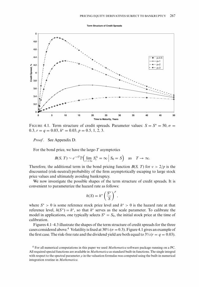
FIGURE 4.1. Term structure of credit spreads. Parameter values: S = S∗ = 50, σ =0.3, r = q = 0.03, h∗ = 0.03, p = 0.5, 1, 2, 3.


For the bond price, we have the large-T asymptotics

B(S, T ) ∼ e−rTP(

limt→∞ S�

t = ∞∣∣∣ S0 = S

)as T → ∞.

Therefore, the additional term in the bond pricing function B(S, T) for ν > 2/p is thediscounted (risk-neutral) probability of the firm asymptotically escaping to large stockprice values and ultimately avoiding bankruptcy.

We now investigate the possible shapes of the term structure of credit spreads. It isconvenient to parameterize the hazard rate as follows:

h(S) = h∗(

S∗

S

)p

,

where S∗ > 0 is some reference stock price level and h∗ > 0 is the hazard rate at thatreference level, h(S ∗) = h∗, so that h∗ serves as the scale parameter. To calibrate themodel in applications, one typically selects S∗ = S0, the initial stock price at the time ofcalibration.

Figures 4.1–4.3 illustrate the shapes of the term structure of credit spreads for the threecases considered above.4 Volatility is fixed at 30% (σ = 0.3). Figure 4.1 gives an example ofthe first case. The risk-free rate and the dividend yield are both equal to 3% (r = q = 0.03).

4 For all numerical computations in this paper we used Mathematica software package running on a PC.All required special functions are available in Mathematica as standard built-in functions. The single integralwith respect to the spectral parameter ρ in the valuation formulas was computed using the built-in numericalintegration routine in Mathematica.

268 V. LINETSKY


3

3.5

4

4.5

5

5.5

6

6.5

7

0 5 10 15 20 25 30 35 40 45 50


Cre

dit

Sp

read

, %

p=0.5

p=1

p=2

p=3

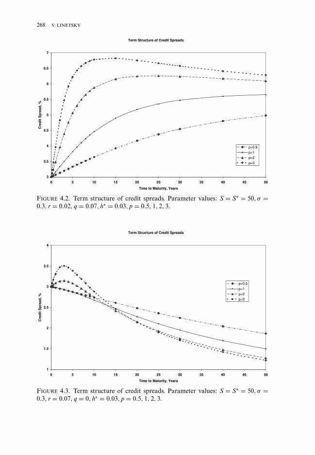
FIGURE 4.2. Term structure of credit spreads. Parameter values: S = S∗ = 50, σ =0.3, r = 0.02, q = 0.07, h∗ = 0.03, p = 0.5, 1, 2, 3.


1

1.5

2

2.5

3

3.5

4

0 5 10 15 20 25 30 35 40 45 50


Cre

dit

Sp

read

, %

p=0.5

p=1

p=2

p=3

FIGURE 4.3. Term structure of credit spreads. Parameter values: S = S∗ = 50, σ =0.3, r = 0.07, q = 0, h∗ = 0.03, p = 0.5, 1, 2, 3.


In this case |r − q| ≤ σ 2/2 and the asymptotic spread is S∞ = 0.01125 (112.5 basispoints). Figure 4.1 plots four curves corresponding to the four choices of the hazardrate parameter p = 0.5, 1, 2, 3 with h∗ = 0.03 and S∗ = 50. For these parameter values,the term structure has a humped shape, first upward slopping and then slowly downwardslopping toward the asymptotic yield.

Figure 4.2 gives an example of the second case with r=0.02 and q=0.07. In this case q >

r + σ 2/2 and the asymptotic spread is S∞ = 0.05 (500 basis points). Figure 4.2 plots fourcurves corresponding to the four choices of the hazard rate parameter p = 0.5, 1, 2, 3 withh∗ = 0.03 and S∗ = 50. The term structures are upward slopping, have a hump, and thendecline toward the asymptotic spread of 5%, which is much larger than that in Figure 4.1since the dividend yield is q > r + σ 2/2.

Figure 4.3 gives an example of the third case with r = 0.07 and q = 0. In this case r >

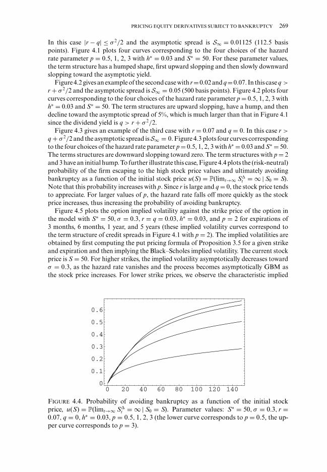
q + σ 2/2 and the asymptotic spread isS∞ = 0. Figure 4.3 plots four curves correspondingto the four choices of the hazard rate parameter p = 0.5, 1, 2, 3 with h∗ = 0.03 and S∗ = 50.The terms structures are downward slopping toward zero. The term structures with p = 2and 3 have an initial hump. To further illustrate this case, Figure 4.4 plots the (risk-neutral)probability of the firm escaping to the high stock price values and ultimately avoidingbankruptcy as a function of the initial stock price u(S) = P(limt→∞ S�

t = ∞ | S0 = S).Note that this probability increases with p. Since r is large and q = 0, the stock price tendsto appreciate. For larger values of p, the hazard rate falls off more quickly as the stockprice increases, thus increasing the probability of avoiding bankruptcy.

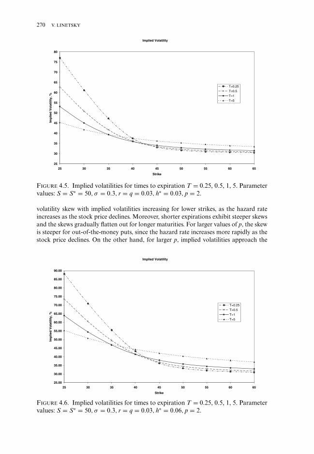
Figure 4.5 plots the option implied volatility against the strike price of the option inthe model with S∗ = 50, σ = 0.3, r = q = 0.03, h∗ = 0.03, and p = 2 for expirations of3 months, 6 months, 1 year, and 5 years (these implied volatility curves correspond tothe term structure of credit spreads in Figure 4.1 with p = 2). The implied volatilities areobtained by first computing the put pricing formula of Proposition 3.5 for a given strikeand expiration and then implying the Black–Scholes implied volatility. The current stockprice is S = 50. For higher strikes, the implied volatility asymptotically decreases towardσ = 0.3, as the hazard rate vanishes and the process becomes asymptotically GBM asthe stock price increases. For lower strike prices, we observe the characteristic implied

0 20 40 60 80 100 120 1400

0.1

0.2

0.3

0.4

0.5

0.6

FIGURE 4.4. Probability of avoiding bankruptcy as a function of the initial stockprice, u(S) = P(limt→∞ S�

t = ∞ | S0 = S). Parameter values: S∗ = 50, σ = 0.3, r =0.07, q = 0, h∗ = 0.03, p = 0.5, 1, 2, 3 (the lower curve corresponds to p = 0.5, the up-per curve corresponds to p = 3).

270 V. LINETSKY

Implied Volatility

25

30

35

40

45

50

55

60

65

70

75

80

25 30 35 40 45 50 55 60 65

Strike

Imp

lie

d V

ola

tili

ty,

%

T=0.25

T=0.5

T=1

T=5

FIGURE 4.5. Implied volatilities for times to expiration T = 0.25, 0.5, 1, 5. Parametervalues: S = S∗ = 50, σ = 0.3, r = q = 0.03, h∗ = 0.03, p = 2.

volatility skew with implied volatilities increasing for lower strikes, as the hazard rateincreases as the stock price declines. Moreover, shorter expirations exhibit steeper skewsand the skews gradually flatten out for longer maturities. For larger values of p, the skewis steeper for out-of-the-money puts, since the hazard rate increases more rapidly as thestock price declines. On the other hand, for larger p, implied volatilities approach the

Implied Volatility

25.00

30.00

35.00

40.00

45.00

50.00

55.00

60.00

65.00

70.00

75.00

80.00

85.00

90.00

25 30 35 40 45 50 55 60 65

Strike

Imp

lie

d V

ola

tili

ty,

%

T=0.25

T=0.5

T=1

T=5

FIGURE 4.6. Implied volatilities for times to expiration T = 0.25, 0.5, 1, 5. Parametervalues: S = S∗ = 50, σ = 0.3, r = q = 0.03, h∗ = 0.06, p = 2.


bankruptcy-free volatility σ more rapidly for out-of-the-money calls, as the hazard ratefalls off more rapidly as the stock price increases. For smaller p, the skew is flatter, butdeclines toward the bankruptcy-free σ slower.

Figure 4.6 plots implied volatility skews for the case with h∗ = 0.06. We observe that asthe hazard rate parameter h∗ increases, the skews become steeper. We thus have a clear linkbetween the hazard rate of bankruptcy and resulting credit spreads and option impliedvolatility skews. Increasing probability of bankruptcy of the underlying firm increases bothcredit spreads on corporate bonds and implied volatility skews in stock options.

5. CONCLUSION

In this paper we have solved in closed form a parsimonious extension of the Black–Scholes–Merton model with bankruptcy where the hazard rate of bankruptcy is a neg-ative power of the stock price. By combining a scale change and a measure change, wereduced the model dynamics to a linear stochastic differential equation, whose solutionis a diffusion process that has played a central role in the pricing of Asian options. Thesolution is in the form of a spectral expansion associated with the diffusion infinitesimalgenerator. Pricing formulas for both corporate bonds and stock options are obtainedin closed form. Term credit spreads on corporate bonds and implied volatility skews ofstock options are closely linked in this model, with parameters of the hazard rate speci-fication controlling both the shape of the term structure of credit spreads and the slopeof the implied volatility skew. The results of our analysis provide further insights intothe linkage between corporate credit spreads and volatility skews in stock options. Ouranalytical formulas are easy to implement and, it is hoped, will prove useful to researchersand practitioners in corporate debt and equity derivatives markets.

To conclude, we note that credit risk is not the only cause of implied volatility skewsin equity options. Stochastic volatility σ that is negatively correlated with the stock priceprocess will further contribute to the steepening of the skew. In this paper we kept σ

constant to focus on the credit risk aspect of the problem. Carr and Linetsky (2005)study a jump-to-default extension of the constant elasticity of variance (CEV) model,where σ is a function the underlying stock price.

APPENDIX A: MATHEMATICAL ORIGINS OF THE DENSITY p(ν):BROWNIAN EXPONENTIAL FUNCTIONALS, SCHRODINGER OPERATOR

WITH MORSE POTENTIAL, AND MAASS LAPLACIAN

In this appendix we discuss the mathematical origins of the density p(ν) in Proposition 3.3and provide relevant references. For ν < 0, this density was first obtained by Wong (1964,p. 271, equation 38) (see also Comtet, Monthus, and Yor [1998] and Linetsky [2004a]).This density is closely related to several classical mathematical objects.

For ν ∈ R, consider the process X (ν) solving the SDE (3.4) and starting at x > 0. Definea new process {Z(ν)

t := 12 ln X (ν)

t , t ≥ 0},

dZ (ν)t =

(ν + 1

2e−2Z (ν)

t

)dt + dBt, Z(ν)

0 = z = 12

ln x.

Let P(ν)z be the law of the process Z(ν) starting at z ∈ R and let PB

z be the law of standardBrownian motion starting at z ∈ R.

272 V. LINETSKY

PROPOSITION A.1. We have the following absolute continuity relationship

dP (ν)z

dPBz

∣∣∣∣∣Ft

= exp{−ν2

2t + ν(Bt − z) − 1

4(e−2Bt − e−2z) −

∫ t

0

(ν − 1

2e−2Bu + 1

8e−4Bu

)du

}.

Proof . This result follows from Girsanov’s theorem. �

Let q(ν)(t; x, y) be the density defined by

q (ν)(t; x, y) := ∂

∂yEB

x

[e− ∫ t

0 ( ν−12 e−2Bu + 1

8 e−4Bu ) du1{Bt≤y}],(A.1)

where B is a standard Brownian motion starting at x. From Proposition A.1 we have

p(ν)(t; x, y) = e− ν22 te

14x − 1

4y

(yx

) ν2

q (ν)(

t;12

ln x,12

ln y)

.

By the Feynman–Kac theorem, the density q(ν)(t; x, y) is the heat kernel of the second-order differential operator

H(ν) = −12

d2

dx2+ ν − 1

2e−2x + 1

8e−4x,

a self-adjoint operator in L2(R). The heat kernel satisfies the heat equation with theoperator H(ν)

H(ν)q = −∂q∂t

with the initial condition q(ν)(0; x, y) = δ(x − y), where δ(·) is Dirac’s delta. Theoperator H(ν) is the well-known Schrodinger operator with Morse potential. The spectralexpansion of the density p(ν) in Proposition 3.3 thus follows from the spectral expansionof the Schrodinger operator with Morse potential. The Schrodinger operator

− d2

dx2 + V(x)

with potential of the form

V(x) = ae−βx + be−2βx

first appeared in quantum mechanics in the classical paper Morse (1929) on the spectraof diatomic molecules. It is closely related to another classical differential operator, theMaass Laplacian or Schrodinger operator on the Poincare upper half-plane in a magneticfield.

Let H2 be the upper half-plane with rectangular coordinates (x, y), x ∈ R, y > 0, andwith the Poincare metric (hyperbolic plane). Consider the Schrodinger operator with auniform magnetic field B, B ∈ R, on H2

HB = −12

y2(

∂2

∂x2+ ∂2

∂y2

)+ iBy

∂

∂x+ B2

2.

This is a −1/2 of the standard Laplace–Beltrami operator on H2 plus magnetic field terms.Introduce a new variable η = − 1

2 ln y. On functions of the form u(x, η) = exp(−i px −12η)v(η) the operator HB reduces to the Schrodinger operator with Morse potential.


Harmonic analysis on the hyperbolic plane can be applied to obtain its spectral repre-sentation.

Thus, the density of linear diffusion (3.4), the density of Brownian motion killed at alinear combination of two Brownian exponential functionals (A.1), the heat kernel of theSchrodinger operator with Morse potential, and the heat kernel of the Maass Laplacianon the hyperbolic plane are closely related. These connections have been explored inAlili and Gruet (1997), Alili, Matsumoto, and Shiraishi (2001), Comtet (1987), Comtetand Monthus (1996), Comtet, Monthus, and Yor (1998), Grosche (1988), and Ikeda andMatsumoto (1999) in several different contexts.

APPENDIX B: CONNECTION WITH ASIAN OPTIONS

The process X (ν) and its density p(ν) are closely related to the problem of pricing arithmeticAsian options. Assume that, under the EMM, the underlying asset price follows a GBMprocess {St = S0 exp(σBt + (r − q − σ 2/2)t), t ≥ 0}. For t > 0, let At be the continuousarithmetic average price, At = t−1

∫ t0 Su du. An Asian call (put) option with strike K >

0 and expiration t > 0 delivers the payoff (AT − K)+((K − AT)+) at T . After standard-izing the problem (see Geman and Yor 1993), it reduces to computing expectations ofthe form E[(A(ν)

τ − k)+](E[(k − A(ν)τ )+]), where τ = σ 2T/4, ν = 2(r − q − σ 2/2)/σ 2, k =

τK/S0, and A(ν)τ is a Brownian exponential functional (see Yor 2001)

A(ν)τ =

∫ τ

0e2(Bu+νu) du.

Dufresne’s identity in law (Dufresne 1989, 1990; see also Donati-Martin, Ghomrasni,and Yor 2001) states that, for each fixed t > 0,

A(ν)t

(law)= X (ν)t ,

where X (ν)t is the diffusion process (3.4) starting at the origin. To see this, recall equa-

tion (3.3) (in this case x = 0). By invariance to time reversal of Brownian motion, foreach fixed t > 0

X (ν)t =

∫ t

0e2(Bt−Bu )+2ν(t−u)du

(law)=∫ t

0e2(Bs+νs) ds = A(ν)

t .

Dufresne’s identity in law was applied to the valuation of Asian options by Donati-Martin, Ghomrasni, and Yor (2001). To compute the Asian option price, these authorsobserve that this computation is equivalent to the computation of the price of an optionwritten on the process X (ν) starting at the origin. They compute the resolvent kernel ofX (ν) and, on integration with the payoff, obtain the Laplace transform of the option pricewith respect to time to expiration. This gives an alternative derivation of the celebratedGeman and Yor (1992, 1993) Laplace transform result (which was originally obtainedvia Lamperti’s identity and the theory of Bessel processes). To recover the Asian optionprice for fixed time to expiration, one needs to invert the Laplace transform. The Laplaceinversion for Asian options is accomplished in Linetsky (2004a) by means of the spectralexpansion approach.

APPENDIX C: CONFLUENT HYPERGEOMETRIC FUNCTIONS

This appendix collects some facts about the confluent hypergeometric functions. Thereader is referred to Slater (1960), Buchholz (1969), Abramowitz and Stegun (1972), and

274 V. LINETSKY

Prudnikov, Brychkov, and Marichev (1990) for further details. All the special functionsin this Appendix are available as built-in functions in Mathematica and Maple softwarepackages. To compute these functions efficiently, these packages use a variety of integraland asymptotic representations given in the above references, in addition to the defininghypergeometric series presented here.

The Kummer confluent hypergeometric function is defined by the hypergeometric series

1 F1[a; b; z] =∞∑

n=0

(a)n

(b)n

zn

n!,

where (a)0 = 1, (a)n = a(a + 1) · · · (a + n − 1) are the Pochhammer symbols, (a)n =�(a + n)/�(a), where �(z) is the Gamma function. The regularized Kummer function1F1[a; b; z]/�(b) is an analytic function of a, b, and z, and is defined for all values of a, b,and z real or complex. The second confluent hypergeometric function (Tricomi function)is defined by

U(a, b, z) = π

sin(πb)

{1 F1[a; b; z]

�(1 + a − b)�(b)− z1−b

1 F1[1 + a − b; 2 − b; z]�(a)�(2 − b)

}.

It is analytic for all values of a, b, and z real or complex even when b is zero or a negativeinteger, for in these cases it can be defined in the limit b → ±n or 0. It has the followingsymmetry property

U(a, b, z) = z1−bU(1 + a − b, 2 − b, z).

The confluent hypergeometric functions are solutions of the confluent hypergeometricequation

zd2udz2

+ (b − z)dudz

− au = 0.(C.1)

The first Whittaker function is defined by

Mκ,μ(z) = zμ+1/2e−z/21 F1[1/2 + μ − κ; 1 + 2μ; z].

The regularized Whittaker function

Mκ,μ(z) = Mκ,μ(z)�(1 + 2μ)

(C.2)

is analytic for all values of κ, μ, and z real or complex. The second Whittaker function isdefined by

Wκ,μ(z) = zμ+1/2e−z/2U(1/2 + μ − κ, 1 + 2μ, z)

= π

sin(2μπ )

{ Mκ,−μ(z)�(1/2 + μ − κ)

− Mκ,μ(z)�(1/2 − μ − κ)

}(C.3)

and is analytic for all values of k, μ, and z real or complex, and is even in its second index,

Wκ,−μ(z) = Wκ,μ(z).

Whittaker functions Mκ,μ(z) and W κ,μ(z) are the two solutions of the Whittaker dif-ferential equation

wzz +

⎛⎜⎝−14

+ κ

z+

14

− μ2

z2

⎞⎟⎠ w = 0(C.4)


with the Wronskian

Wκ,μ(z)M′κ,μ(z) − Mκ,μ(z)W ′

κ,μ(z) = 1�(μ − κ + 1/2)

.(C.5)

When κ = μ + n + 12 , n = 0, 1, 2, . . . , the Wronskian vanishes and the functionsMκ,μ(z)

and Wκ,μ(z) become linearly dependent and reduce to generalized Laguerre polynomials(Buchholz 1969, p. 214)

Mμ+n+ 12 ,μ(z) = n!

�(2μ + n + 1)e− z

2 zμ+ 12 L(2μ)

n (z),(C.6)

Wμ+n+ 12 ,μ(z) = (−1)nn!e− z

2 zμ+ 12 L(2μ)

n (z).(C.7)

The following integrals with Whittaker functions are used in the proofs of bond andoption pricing formulas:

∫ x

0zα−1e− z

2 Mκ,μ(z) dz = xα+μ+1/2

α + μ + 1/2

× 2 F2[α + μ + 1/2, 1/2 + κ + μ; α + μ + 3/2, 2μ + 1; −x]

(C.8)

for x > 0 and (α + μ + 1/2) > 0 (Prudnikov, Brychkov, and Marichev 1990, p. 39,equation (1.13.1.1)),

∫ ∞

xzα−1e− z

2 Wκ,μ(z) dz = �(α + μ + 1/2)�(α − μ + 1/2)�(α − κ + 1)

− xα+μ+1/2

α + μ + 1/2�(−2μ)

�(1/2 − κ − μ)

× 2 F2[α + μ + 1/2, 1/2 + κ + μ; α + μ + 3/2, 2μ + 1; −x]

− xα−μ+1/2

α − μ + 1/2�(2μ)

�(1/2 − κ + μ)

× 2 F2[α − μ + 1/2, 1/2 + κ − μ; α − μ + 3/2, −2μ + 1; −x]

(C.9)

for x > 0 (Prudnikov, Brychkov, and Marichev 1990, p. 40, equation (1.13.2.2)),∫ ∞

0zα−1e− z

2 Wκ,μ(z) dz = �(α + μ + 1/2)�(α − μ + 1/2)�(α − κ + 1)

(C.10)

for (α) > | (μ)| − 1/2 (Prudnikov, Brychkov, and Marichev 1990, p. 256, equa-tion (2.19.3.7)), and indefinite integrals (Prudnikov, Brychkov, and Marichev 1990,pp. 39–40, equations (1.13.1.6) and (1.13.2.6))∫

zκ−2e− z2 Wκ,μ(z) dz = −zκ−1e− z

2 Wκ−1,μ(z),(C.11)

∫zκ−2e− z

2 Mκ,μ(z) dz = 1κ + μ − 1/2

zκ−1e− z2 Mκ−1,μ(z).(C.12)

276 V. LINETSKY

The generalized hypergeometric function is defined by

2 F2[a1, a2; b1, b2; z] =∞∑

n=0

(a1)n(a2)n

(b1)n(b2)n

zn

n!.(C.13)

The regularized function 2F2[a1, a2; b1, b2; z]/(�(b1)�(b2)) is analytic for all values ofa1, a2, b1, b2, and z real or complex.

The following integrals with Laguerre polynomials are used in the proofs of pricingformulas: ∫ ∞

0xα−1e−xL(ν)

n (x) dx = (ν − α + 1)n

n!�(α)(C.14)

for (α) > 0 (Prudnikov, Brychkov, and Marichev 1986, p. 463, equation (2.19.3.5)),∫ ∞

xzα−1e−z L(ν)

n (z) dz = (ν − α + 1)n

n!�(α)

− (ν + 1)n

n!xα

α2 F2[ν + n + 1, α; ν + 1, α + 1; −x]

(C.15)

for x > 0 (Prudnikov, Brychkov, and Marichev 1986, p. 51, equation (1.14.3.7)), and theindefinite integral (Prudnikov, Brychkov, and Marichev 1986, p. 51, equation (1.14.3.9))∫

zν+n−1e−z L(ν)n (z) dz = 1

nzν+ne−z L(ν)

n−1(z).(C.16)

APPENDIX D: PROOFS

Proof of Proposition 3.2 (Donati-Martin, Ghomrasni, and Yor 2001). It is classical(Ito and McKean 1974) that, for s > 0, the resolvent kernel can be taken in the form

Gs(x, y) = w −1s m(y)ψs(x ∧ y)φs(x ∨ y),(D.1)

where the functions ψ s(x) and φs(x) can be characterized as the unique (up to a multipleindependent of x) solutions of the ODE

2x2u′′(x) + [2(ν + 1)x + 1]u′(x) = su(x)(D.2)

by demanding that ψ s is increasing and φs is decreasing (Borodin and Salminen 2002,p. 18). These functions have the following limits at zero and infinity (Borodin and Salminen2002, pp. 18–19)). At the entrance boundary at zero: ψs(0+) > 0, φs(0+) = ∞. At thenatural boundary at infinity: ψs(∞) = +∞, φs(∞) = 0. The functions ψ s(x) and φs(x)are linearly independent for all s > 0. Moreover, the Wronskian ws with respect to thescale density s(x) defined by

φs(x)ψ ′s(x) − ψs(x)φ′

s(x) = s(x)ws

is independent of x.We look for solutions to (D.2) in the form

u(x) = x1−ν

2 e1

4x w(

12x

)(D.3)

for some function w(z). Substituting this functional form into equation (D.2), we arriveat the Whittaker equation (C.4) for w , where κ = (1 − ν)/2 and μ = μ(s) = 1

2

√2s + ν2.

For s > 0, the two linearly independent solutions are Mκ,μ(z) and W κ,μ (z) with the


Wronskian (C.5). Thus, the solutions ψs(x) and φs(x) of the original problem can betaken in the form

ψs(x) = x1−ν

2 e1

4x W1−ν2 ,μ(s)

(1

2x

), φs(x) = x

1−ν2 e

14x M 1−ν

2 ,μ(s)

(1

2x

).(D.4)

The boundary properties are verified using the asymptotic properties of the Whittakerfunctions for z > 0 and μ > 0

Mκ,μ(z) ∼ 1�(1 + 2μ)

zμ+ 12 e− z

2 and Wκ,μ(z) ∼ �(2μ)� (μ − κ + 1/2)

z−μ+ 12 e− z

2 as z → 0,

(D.5)

Mκ,μ(z) ∼ 1� (1/2 + μ − κ)

z−κez2 and Wκ,μ(z) ∼ zκe− z

2 as z → ∞.(D.6)

From (C.5), the Wronskian with respect to the scale density is

ws = 12�(μ(s) + ν/2)

.(D.7)

Substituting (D.4) and (D.7) into (D.1), we arrive at (3.10). The case x = 0 is obtained inthe limit x → 0, using the asymptotic properties of the Whittaker functions (D.6). �

Proof of Proposition 3.3. Following the complex variable approach to spectral expan-sions (see Titchmarsh 1962), we analytically invert the Laplace transform (3.9) with theresolvent kernel (3.10). Regarded as a function of complex variable s ∈ C, the resolventkernel (3.10) has the following singularities. For ν < 0, it has simple poles at

s = sn = −λn, λn = 2n(|ν| − n), n = 0, 1, . . . , [|ν|/2],(D.8)

(poles of the Gamma function in (3.10) at μ(−λn) + ν/2 = −n, n = 0, 1, . . . , [|ν|/2],where [x] denotes the integer part of x). The residues at these poles are

Ress=−λn Gs(x, y)

= (−1)n 2(|ν| − 2n)n!

e1

4x − 14y

(yx

) ν−12

M 1−ν2 ,− ν

2 −n

(1

2(x ∨ y)

)W1−ν

2 ,− ν2 −n

(1

2(x ∧ y)

)

= 2(|ν| − 2n)n!�(1 + |ν| − n)

e− 12y

(1

2x

)−n (1

2y

)1+|ν|−n

L(|ν|−2n)n

(1

2x

)L(|ν|−2n)

n

(1

2y

).

(D.9)

The second equality follows from the reduction of the Whittaker functions to generalizedLaguerre polynomials when the difference between the two indexes is a positive half-integer (equations (C.6) and (C.7)). Furthermore, for all real ν, the resolvent has a branchpoint at s = −ν2/2. We place the branch cut from s = −ν2/2 to s → −∞ on the negative

278 V. LINETSKY

real axis. It is convenient to parameterize the branch cut as {s = −(ρ2 + ν2)/2, ρ ≥ 0}.The jump across the branch cut is

G 12 (ν2+ρ2)eiπ (x, y) − G 1

2 (ν2+ρ2)e−iπ (x, y)

= −e1

4x − 14y

(yx

) ν−12

W1−ν2 ,

iρ2

(1

2(x ∧ y)

) {�

(ν − iρ

2

)M 1−ν

2 ,− iρ2

(1

2(x ∨ y)

)− �

(ν + iρ

2

)M 1−ν

2 ,iρ2

(1

2(x ∨ y)

)}

= − iπ

e1

4x − 14y

(yx

) ν−12

W1−ν2 ,

iρ2

(1

2x

)W1−ν

2 ,iρ2

(1

2y

) ∣∣∣∣� (ν + iρ

2

)∣∣∣∣2

sinh(πρ).

(D.10)

In the first equality we used the fact that W κ,μ (z) is even in its second index. In the secondequality we used equation (C.3).

To recover the transition density, we invert the Laplace transform (3.9). The Bromwichcomplex inversion formula reads for t > 0

p(t; x, y) = 12π i

∫ c+i∞

c−i∞estGs(x, y) ds,

where the integration is performed along the contour Re(s) = c for some c > 0. Thisintegral is calculated by applying the Cauchy Residue Theorem (see Titchmarsh 1962):

p(t; x, y) = 1{ν<0}[|ν|/2]∑n=0

esntRess=sn Gs(x, y)

− 12π i

∫ ∞

0e− (ν2+ρ2)t

2

{G 1

2 (ν2+ρ2)eiπ (x, y) − G 12 (ν2+ρ2)e−iπ (x, y)

}ρ dρ.

(D.11)

Substituting (D.9) and (D.10) in (D.11), we arrive at the spectral representation for thedensity (3.12).

Since the boundary at zero is entrance, the limit x → 0 exists and can be explicitly com-puted using the asymptotics of the Whittaker function (D.6) and Laguerre polynomials

limz→∞

(z−n L(α)

n (z)) = (−1)n

n!. �

Proof of Proposition 3.4. First consider the case ν < 2/p (equivalently, r − q − σ 2/2 <

0). Bond payoff ψbond(x) = 1 is such that χψ ∈ H, and the spectral representation (3.13) is

applicable. The integrals in equations (3.14) and (3.15) for χψ (y) = (y/β)−1p are calculated

in closed form by reduction to the known integrals (C.10) and (C.14) for Whittakerfunctions and Laguerre polynomials.

The case ν ≥ 2/p (equivalently, r − q − σ 2/2 ≥ 0) is more involved. For the bondpayoff ψbond(x) = 1, χψ (x) = (x/β)−1/p /∈ H and, hence, the spectral representation(3.13) cannot be applied. The alternative is to first compute the Laplace transform (3.16)


with the resolvent kernel (3.10) and then do the Laplace inversion, choosing the contourof integration in the Laplace inversion formula

eqT S−1 B(S, T ) = E(ν)x

[(X(ν)

τ

/β)−1/p] = 1

2π i

∫ c+i∞

c−i∞esτ�(ν)

s (x) ds(D.12)

to the right of any singularities of �(ν)s (x) in the complex s-plane. The function �

(ν)s (x) is

calculated in closed form by calculating the integral in (3.16), using the known integrals(C.8) and (C.9). We omit the resulting cumbersome expression. In addition to the singu-larities inherited from the resolvent kernel Gs(x, y) (a branch cut from s = −ν2/2 to −∞on the negative real axis for all real ν and poles (D.8) for ν < 0), for ν > 2/p, �

(ν)s (x) has

an additional simple pole at

s = s∗ = −λ∗, λ∗ = 2p

(ν − 1

p

)= 4(r − q)

p2σ 2> 0

that comes from the factor 1/(1/p − ν/2 + μ(s)). The residue at this pole is

Ress=s∗�(ν)s (x) = (x/β)−

1p�(ν − 1/p)�(ν − 2/p)

U(

1p,

2p

− ν + 1,1

2x

),

a strictly positive expression for ν > 2/p.The inversion integral (D.12) is calculated by applying the Cauchy Residue Theorem

as in the proof of Proposition 3.3 (equation (D.11))

E(ν)x

[(X(ν)

τ

/β)−1/p] = 1{ν>2/p}es∗τ Ress=s∗�(ν)

s (x) + 1{ν<0}[|ν|/2]∑n=0

esnτ Ress=sn �(ν)s (x)

− 12π i

∫ ∞

0e− (ν2+ρ2)τ

2

{�

(ν)12 (ν2+ρ2)eiπ (x) − �

(ν)12 (ν2+ρ2)e−iπ (x)

}ρ dρ.

Computing this expression leads to the result in Proposition 3.4 for the bond price, withthe additional pole at s = s∗ resulting in the additional positive term in the bond pricingformula for ν > 2/p. �

Proof of Proposition 3.5. The put payoff ψput(x) = (K − x)+ is such that χψ ∈ H forall ν ∈ R and, hence, the valuation of the put payoff given no bankruptcy (2.6) followsfrom the spectral expansion (3.13). The integrals in the expressions for the expansioncoefficients (3.14) and (3.15) are calculated in closed form by reduction to the knownintegrals (C.9) and (C.15). The recovery part (bankruptcy claim) value (2.7) follows fromthe bond valuation in Proposition 3.4. �

Proof of Proposition 4.1. The function u(S) = P(limt→∞ S�t = ∞ | S0 = S) solves the

ODE (see Karlin and Taylor 1981, Chapter 12)

12σ 2S2uSS + [r − q + αS−p]SuS = αS−pu

subject to the boundary conditions

u(0) = 0, u(∞) = 1.

Introducing a new variable y = 1/(2x), where x = (pσ 2/(4α))Sp as in Section 3, this ODEreduces to the confluent hypergeometric equation (C.1) with

a = 1p, b = 2

p− ν + 1 = 2(q − r )

pσ 2+ 1 + 1

p.

280 V. LINETSKY

The solution satisfying the required boundary conditions is

u(S) = �(ν − 1/p)�(ν − 2/p)

U(

1p,

2p

− ν + 1,1

2x

).

The boundary conditions are verified by using the asymptotic properties of the functionU(a, b, x)

limx→0

U(a, b, x) = �(1 − b)�(1 + a − b)

for b < 1, and

limx→∞ U(a, b, x) = 0

for a > 0. �

REFERENCES

ABRAMOWITZ, M., and I. A. STEGUN (1972): Handbook of Mathematical Functions. New York:Dover.

ALILI, L., and J.-C. GRUET (1997): An Explanation of a Generalized Bougerol’s Identity in Termsof Hyperbolic Brownian Motion, in Exponential Functionals and Principal Values Related toBrownian Motion, M. Yor, ed. Biblioteca de la Revista Matematica Iberoamericana, Madrid.

ALILI, L., H. MATSUMOTO, and T. SHIRAISHI (2001): On a Triplet of Exponential BrownianFunctionals, Sem. de Prob., xxxv, Springer, Berlin, 396–415.

ANDERSEN, L., and D. BUFFUM (2003/2004): Calibration and Implementation of ConvertibleBond Models, J. Comput. Finance 7(2), 1–34.

AYACHE, E., P. FORSYTH, and K. VETZAL (2003): The Valuation of Convertible Bonds with CreditRisk, J. Derivatives 11(Fall), 9–29.

BIELECKI, T., and M. RUTKOWSKI (2002): Credit Risk: Modeling, Valuation and Hedging. Berlin:Springer.

BORODIN, A. N., and P. SALMINEN (2002): Handbook of Brownian Motion, 2d ed. Boston:Birkhauser.

BUCHHOLZ, H. (1969): The Confluent Hypergeometric Function. Berlin: Springer.

CARR, P., and A. JAVAHERI (2005): The Forward PDE for European Options on Stocks withFixed Fractional Jumps, Int. J. Theoret. Appl. Finance 8(2), 239–253.

CARR, P., and V. LINETSKY (2005): A Jump-to-Default Extended Constant Elasticity of VarianceModel: An Application of Bessel Processes, Working Paper.

COMTET, A. (1987): On the Landau Levels on the Hyperbolic Space, Ann. Phys. 173, 185–209.

COMTET, A., and C. MONTHUS (1996): Diffusion in a One-Dimensional Random Medium andHyperbolic Brownian Motion, J. Phys. A 29, 1331–1345.

COMTET, A., C. MONTHUS, and M. YOR (1998): Exponential Functionals of Brownian Motionand Disordered Systems, J. Appl. Prob. 35, 255–271.

DAVIS, M., and F. LISCHKA (2002): Convertible Bonds with Market Risk and Credit Risk, inApplied Probability, R. Chan et al., eds. Studies in Advanced Mathematics. Providence, RI:American Mathematical Society/International Press, 45–58.

DONATI-MARTIN, C., R. GHOMRASNI, and M. YOR (2001): On Certain Markov Procsses Attachedto Exponential Functionals of Brownian Motion: Applications to Asian Options, RevistaMatematica Iberoamericana, 17(1), 179–193.


DUFFIE, D., M. SCHRODER, and C. SKIADAS (1996): Recursive Valuation of Defaultable Securitiesand the Timing of Resolution of Uncertainty, Ann. Appl. Prob. 6, 1075–1096.

DUFFIE, D., and K. SINGLETON (1999): Modeling Term Structures of Defaultable Bonds, Rev.Financial Stud. 12, 653–686.

DUFFIE, D., and K. SINGLETON (2003): Credit Risk. Princeton, NJ: Princeton University Press.

DUFRESNE, D. (1989): Weak Convergence of Random Growth Processes with Applications toInsurance, Insur. Math. Econ. 8, 187–201.

DUFRESNE, D. (1990): The Distribution of a Perpetuity, with Applications to Risk Theory andPension Funding, Scand. Actuar. J. 1990, 39–79.

GEMAN, H., and M. YOR (1992): Some Relations between Bessel Processes, Asian Options andConfluent Hypergeometric Functions, C.R. Acad. Sci., Paris, Ser. I 314, 471–474 (Englishtranslation reprinted in Yor, M., 2001, Exponential Functionals of Brownian Motion and Re-lated Processes. Berlin: Springer.).

GEMAN, H., and M. YOR (1993): Bessel Processes, Asian Options and Perpetuities, Math. Finance3, 349–375.

GOROVOI, V., and V. LINETSKY (2004): Black’s Model of Interest Rates as Options, EigenfunctionExpansions, and Japanese Interest Rates, Math. Finance 14, 49–78.

GROSCHE, C. (1988): The Path Integral on the Poincare Upper Half Plane with a Magnetic Fieldand for the Morse Potential, Ann. Phys. 187, 110–134.

HULL, J., I. NELKEN, and A. WHITE (2004): Merton’s Model, Credit Risk, and Volatility Skews,Working Paper, University of Toronto.

IKEDA, N., and H. MATSUMOTO (1999): Brownian Motion on the Hyperbolic Plane and SelbergTrace Formula, J. Funct. Anal. 163, 63–110.

IKEDA, N., and S. WATANABE (1981): Stochastic Differential Equations and Diffusion Processes.Amsterdam: North-Holland.

ITo, K., and H. MCKEAN, (1974): Diffusion Processes and Their Sample Paths. Berlin: Springer.

JACKWERTH, J. C., and M. RUBINSTEIN (1996): Recovering Probability Distributions from OptionPrices, J. Finance 51, 62–74.

JARROW, R., D. LANDO, and S. TURNBULL (1997): A Markov Model for the Term Structure ofCredit Risk Spreads, Rev. Financial Stud. 10, 481–523.

JARROW, R., and S. TURNBULL (1995): Pricing Derivatives on Financial Securities Subject toCredit Risk, J. Finance 50(1), 53–85.

JEANBLANC, M., M. YOR, and M. CHESNEY (2006): Mathematical Methods for Financial Markets.Berlin: Springer.

KARATZAS, I., and S. SHREVE (1992): Brownian Motion and Stochastic Calculus. New York:Springer-Verlag.

KARLIN, S., and H. M. TAYLOR (1981): A Second Course in Stochastic Processes. San Diego:Academic Press.

LANDO, D. (2004): Credit Risk Modeling. Princeton, NJ: Princeton University Press.

LEWIS, A. (1998): Applications of Eigenfunction Expansions in Continuous-Time Finance,Math. Finance 8, 349–383.

LINETSKY, V. (2004a): Spectral Expansions for Asian (Average Price) Options, Operat. Res. 52(6),856–867.

LINETSKY, V. (2004b): The Spectral Decomposition of the Option Value, Int. J. Theoret. Appl.Finance 7(3), 337–384.

LINETSKY, V. (2004c): Lookback Options and Diffusion Hitting Times: A Spectral ExpansionApproach, Finance Stochast. 8(3), 373–398.

282 V. LINETSKY

LINETSKY, V. (2004d): The Spectral Representation of Bessel Processes with Constant Drift:Applications in Queueing and Finance, J. Appl. Prob. 41(2), 327–344.

LINETSKY, V. (2006): Spectral Methods in Derivatives Pricing, in Handbook of Financial Engi-neering, J. R. Birge and V. Linetsky, eds. Amsterdam: Elsevier.

MADAN, D., and H. UNAL (1998): Pricing the Risk of Default, Rev. Deriv. Res. 2, 121–160.

MCKEAN, H. (1956): Elementary Solutions for Certain Parabolic Partial Differential Equations,Transactions of the American Mathematical Society 82, 519–548.

MORSE, P. M. (1929): Diatomic Molecules According to the Wave Mechanics, II: VibrationalLevels, Phys. Rev. 34, 57–64.

MUROMACHI, Y. (1999): The Growing Recognition of Credit Risk in Corporate and FinancialBond Markets, Working Paper, NLI Research Institute.

PESKIR, G. (2004): On the Fundamental Solution of the Kolmogorov-Shiryaev Equation, Re-search Report No. 438, Aarhus.

PRUDNIKOV, A. P., Y. A. BRYCHKOV, and O. I. MARICHEV (1986): Integrals and Series, Vol. 2.New York: Gordon and Breach.

PRUDNIKOV, A. P., Y. A. BRYCHKOV, and O. I. MARICHEV (1990): Integrals and Series, Vol. 3.New York: Gordon and Breach.

REVUZ, D., and M. YOR (1999): Continuous Martingales and Brownian Motion, 3rd edn. Berlin:Springer.

RUBINSTEIN, M. (1994): Implied Binomial Trees, J. Finance 49, 771–818.

SCHOONBUCHER, P. J. (2003): Credit Derivatives Pricing Models. New York: Wiley.

SHIRYAEV, A. N. (1961): The Problem of the Most Rapid Detection of a Disturbance in aStationary Process, Soviet Mathematics Doklady 2, 795–799.

SLATER, L. J. (1960): Confluent Hypergeometric Functions. Cambridge, UK: Cambridge Univer-sity Press.

TAKAHASHI, A., T. KOBAYASHI, and N. NAKAGAWA (2001): Pricing Convertible Bonds withDefault Risk, J. Fixed Income 11, 20–29.

TITCHMARSH, E. C. (1962): Eigenfunction Expansions Associated with Second-Order DifferentialEquations. Oxford: Clarendon.

WONG, E. (1964): The Construction of a Class of Stationary Markoff Processes, in SixteenthSymposium in Applied Mathematics—Stochastic Processes in Mathematical Physics and En-gineering, R. Bellman, ed. Providence, RI: American Mathematical Society, 264–276.

YOR, M. (2001): Exponential Functionals of Brownian Motion and Related Processes. Berlin:Springer.

PRICING EQUITY DERIVATIVES SUBJECT TO …users.iems.northwestern.edu/~linetsky/default.pdfPRICING...

Documents

Transcript of PRICING EQUITY DERIVATIVES SUBJECT TO …users.iems.northwestern.edu/~linetsky/default.pdfPRICING...