Pricing and Hedging of Japan Equity-Linked Power Reverse Dual Note

Pricing and Hedging of Japan Equity-linked Power Reverse Dual Note Using Least Squares

Monte Carlo Simulation

Frank Fung

Shaoyu Hou

Nicholas Lee

Mayank Rao

Abstract

We computed the price of a structured product, the Japan Equity-linked Power Reverse Dual

note (hereafter referred to as JRD), using a Monte Carlo approach with Least Squares to

account for early exercise. We benchmarked the pricing model on a number of simpler

derivatives with closed form solutions or highly accurate pricing from FD schemes. The

sensitivity of JRD with respect to various parameters and performance from different basis

functions is investigated. We employed quasi-random sequences, latin hypercubes and

Brownian bridges as Variance Reduction techniques. We also hedge the JRD using static and

dynamic delta hedging.

Nomenclature

For illustrative purpose we consider an instance of the product with 8 months until maturity,

2 coupon payments in total (including that at maturity) and monthly observations:

T: Date of maturity

τ: Time interval between two consecutive observation dates t�: The date of the payment of the nth

coupon (n=1 in this case) S�: Stock price of the ith

stock in the basket B�: Knock-out barrier of the ith

stock in the basket

Problem Description

Japan Equity-linked Power Reverse Dual Target Accrual Note (JRD): The JRD is a note targeted

towards Japanese investors wishing to gain exposure to US equity markets. Investors can also

gain exposure to FX via the “power reverse” feature. The note pays off a coupon based on

the best performing stock in a basket of 5 stocks. A detailed definition of terms and product

specifications can be found in the following sections.

Definition of terms:

Power Reverse Dual: Reverse dual notes offer coupons in domestic currency based on a

foreign interest rate. Power reverse dual notes offer FX exposure and are suitable when you

expect the domestic/foreign rate to decline.

The JRD note offers a twist on this standard product by allowing investors to gain equity

exposure instead of just interest rates (which are currently at historic lows and not attractive).

Moreover, the JPY is currently very strong. However given the state of the Japanese economy

relative to the US economy, we expect the JPY to decline - thereby the “power” feature in

the note, which exposes the investor to the FX rate, enhances the yield if the yen declines.

Equity Linked Note: This note pays a coupon on a principle of ¥100 based on the best

performing stock from a basket of 5 stocks.

Up and Out Barrier: If any of the stocks in the underlying basket breach their preset barriers,

the note terminates immediately, and investors a paid a bonus coupon to compensate them

for the early termination.

τ

T t�

Product Specification:

The diagram above illustrates the basic setup of the JRD note. The mechanics are as follows:

• Investor pays ¥X to the issuing bank

• Principal is protected, but subject to FX risk.

• On an annual basis, the investor receives ¥ Y*JPYUSD from the bank. Here Y is

calculated as:

� � �� − �� , 0� ∗ 100 ∀� Here �� is the stock prices of stock i on each observation day; �� is the stock

price of stock i at the beginning of the coupon interval and �� is the strike price for

stock i

• The JPYUSD exchange rate is calculated on the day of any cashflow.

• If any of the stocks �� in the basket hits their “knock out barrier” ��, the note is

terminated, and the investor is paid a bonus coupon

• �� is checked on each observation day.

• After 1 year, if the note has not been redeemed or called, the note terminates and

the investor received his final coupon on a notional of ¥100 (the basic pricing unit for

the JRD)

• On any of the observation dates, the investor can call the product. If the product is

called the investor will be paid a coupon linked to the highest performing asset as of

the exercise date (only in the Bermudan version of the JRD)

Pricing a product with early exercise features is a complicated exercise when using Monte

Carlo simulation. A simple way to do this would be to simulate entire trajectories, and then

at each point consider exercising versus holding on. However the price obtained by following

this procedure will be biased upwards, as it is a “perfect foresight” estimate of the price. In

reality we do not know what the optimal exercise decision will be. Longstaff and Schwartz[1]

present a technique based on a least squares regression that allows you to make a decision

for early exercise based on the conditional expectation of the underlying asset price. This

technique requires the use of basis functions that are capable of expressing information

Investor

Issuer

Basket of

5 stocks

X JPY

Y*JPYUSD Y=Best of 5

Equity exposure

about the underlying prices that can then be used in an ordinary least squares regression to

generate conditional expectations. There is no hard and fast rule for the choice of basis

functions, and we need to experiment with various kinds of functions to determine a good fit.

In this paper we experiment with various kinds of functions (Monomials, Laguerre, Bessel,

Hermite and Chebyshev). We pick a function that best captures the behavior of the JRD

under various scenarios.

To focus on the simulation and the analysis of our product, we decide to use a simple

geometric Brownian motion model for the stock and FX dynamics, namely dS� = �r − y�"S�dt + σ�S�dW� �1" dQ = �r& − r "Qdt + σ'QdW' �2"

with the correlation matrix for the Brownian motions (5 stocks, and 1 FX rate which is

assumed to be uncorrelated to any of the stocks hence has zero entries at all places except a

‘correlation’ of 1 with itself)

ρ) =*++,

1ρ�.ρ./ρ/0ρ010

ρ.�1ρ./ρ.0ρ.10

ρ/�ρ/.1ρ/0ρ010

ρ0�ρ0.ρ0/1ρ010

ρ1�ρ1.ρ1/ρ1010

0000012334 �3"

here r is the foreign risk-free rate, y� is the dividend yield for the ith

stock, σ� is the

volatility of the ith

stock, r& is the domestic risk-free rate and σ' is the volatility of the

6789:;<= =>??9@=AB7?9<C@ =>??9@=A FX rate. Considering the complexity in the structure, we will assume a

constant flat yield curve throughout.

In this paper we consider we have a basket of 5 stocks whose correlation matrix we derived

from historical data. The correlation matrix along with the other parameters can be found in

Appendix A.

Methodology

Here we briefly describe how we priced the product including the least squares regression.

Equity Linked option: Using cholesky decomposition, we generate correlated weiner

processes. These processes are used to simulate stock trajectories. At each observation date

we consider a payout based on the best performing stock if the exercise cashflow is greater

than the conditional expectation of the stock prices at that point (from the Least Squares

regression)

Barrier Option: through matrices “stillAlive” and “breachingPoint” we keep of track of when

the barrier was breached by any stock

Power Reverse Dual (PRDC): Each cashflow is multiplied by the corresponding FX rate which

is also simulated at each point

Pricing on intermediate dates: This feature allows us to dynamically hedge the product. To

handle this, we divide the maturity into intervals and calculate the number of intervals

remaining in each coupon.

Least Squares Regression: At each observation date we determine the conditional

expectation of future prices by regressing the current stock prices against some basis

functions. This is further discussed in the “Basis Functions” section.

Benchmarking

We benchmarked our pricing function against several sources.

1) The basket call from Tavella [2] page 200: This example has a benchmark that was

obtained by running a high quality finite differencing scheme on a basket of 3 assets.

There are no barriers or other exotic features. The results obtained are shown in

Table 1

Exercise

Opportunities

Benchmark JRD

Pricer

Error Diff against

Benchmark

10 17.844 17.782 0.18 -0.062

15 17.969 17.891 0.13 -0.078

30 18.082 17.949 0.18 -0.133

Table 1: Benchmarking against basket of 3 assets from FD scheme[2]

2) Benchmarking against options with analytical results: To validate the JRD’s rainbow,

barrier and FX features, we benchmark our product with simpler derivatives where

analytical solutions are available.

We implemented general closed form pricing models for options contingent to the

maximum or the minimum of any number of assets using the result by Johnson[4].

With respect to the barrier feature, since our product has a discrete barrier which

does not have a closed form solution, we benchmarked our result to a continuous

barrier option’s analytical solution, with displaced barrier as suggested by Broadie

and Glasserman[5].

Theoretical value JRD Pricer

Rainbow option 13.243 13.288

Barrier option (pricing from adjusted

continuous barrier)

3.4371 3.4512

Quanto option 4.1075 4.1409

Table 2: Benchmarking against Analytical option prices

3) Benchmarking against European structures: Another way to benchmark a pricing

function is to consider the European version of the product and the Bermudan

premium. This premium is discussed more extensively in the “European versus

Bermudan structures” section.

Results and Discussion

For pricing the Bermudan JRD note, we utilized Monte Carlo simulations with the Least

Squares approach for early exercise. We also experimented with several variance reduction

techniques to accelerate the pricing over the naïve MC approach. We discuss these

techniques briefly and then present our results.

Quasi-Random Sequences: We implemented the Sobol sequence. In the naïve approach we

sample randomly from a normal distribution. However this approach does not cover the

sample space uniformly and as a result we experience a clustering effect. QRS numbers

rectify this problem. In lower dimensions, QRS numbers cover the sample space relatively

well and therefore lead to more accurate pricing. A problem with QRS numbers is that unlike

the naive approach which has a clearly defined convergence law (and therefore a well

defined termination criterion), convergence is not as well defined. This is primarily because

the theoretical error can be drastically different from the numerical error obtained. It is

therefore good practice to calibrate to the naïve MC. The reader is referred to [2] for further

details on this.

Quasi-Random Sequences with Brownian Bridges: numbers generated from a QRS tend to

work well in low dimensions. As the dimensionality of the problem increases however, the

numbers generated from quasi-random sequences tend to leave gaps. This reduces the

acceleration obtained in higher dimensions. This can be exploited by using Brownian bridges.

The numbers from the lower dimensions can be used at the more important points (end of

the trajectory, mid point of trajectory etc). Each time we add a point using the Brownian

bridge technique, the variance of the new point is reduced by half. We can therefore obtain

significant acceleration in this way. To control the random numbers used in the construction

of the bridge we developed our own implementation of the bridge (rather than use the

default one implemented in MATLAB).

Table 3 shows the results from under different scenarios. The parameters used to obtain

these results are shown in Appendix A. For the Least Squares regression we used 10 Hermite

polynomials on 3 cross products ( �., .. & � .) on the two best performing stocks in the

basket at each observation date.

Naïve Sobol Sobol with BB

Cycles Price Standard

Error

CPU Price Standard

Error

CPU Price Standard

Error

CPU

8 Exercise Opportunities

10000 23.34 0.10656 74 23.31 0.06902 49 23.37 0.045109 47

50000 23.34 0.06056 222 23.37 0.031173 265 23.41 0.020798 268

100000 23.40 0.03715 196 23.38 0.020319 237 23.39 0.014715 252


10000 23.81 0.09871 75 23.97 0.078865 96 23.95 0.056059 102

50000 23.93 0.041052 544 24.01 0.028306 596 23.96 0.021163 615

100000 24.00 0.03370 647 24.00 0.021172 1053 23.94 0.014697 864


10000 24.40 0.09754 96 24.45 0.077832 113 24.38 0.056099 110

50000 24.31 0.06085 807 24.40 0.03699 954 24.38 0.023484 1047

100000 24.37 0.03605 984 24.37 0.022355 990 24.35 0.016417 1000

Table 3: Prices and errors obtained via naïve MC, MC with Sobol and MC with Sobol & Brownian bridges

Depending on the number of exercise opportunities, the JRD has dimensions ranging from 48

to 192 (5 stocks + 1 fx rate times the # of exercise opportunities) in Table 3. The results show

that even though Sobol sequences do reduce the standard error, they are not as effective in

higher dimensions. Adding Brownian bridges however reduces the variance by more than

half in most of the cases.

Latin Hypercube Sampling (LHS): extends the concept from stratified sampling (which

samples from each ‘strata’ in the unit hypercube). LHS is similar except that it samples from

each ‘row’ and ‘column’ in the multi dimensional hypercube such that no cell is repeated. By

increasing the number of cells in the LHS, we can therefore obtain a sequence of random

numbers that cover the sample space better than the standard sampling.

Latin Hypercube Sampling (LHS) with Brownian Bridges: similar to the case with sobol

sequences, we can construct Brownian bridges using random numbers generated from the

LHS.

Using the same setup as before, we price the JRD using LHS. The results are presented in

table 4.

LHS LHS with BB

Cycles Price Standard Error CPU Price Standard Error CPU


10000 23.56 0.077112 694 23.47 0.072128 484

50000 23.39 0.031476 2712 23.43 0.029398 2788


10000 23.93 0.081044 2026 23.91 0.059213 2137

50000 23.99 0.028629 10514 23.98 0.023684 9589


10000 24.39 0.083112 7163 24.40 0.045832 6560

50000 24.39 0.028626 38807 24.39 0.028538 37693

Table 4: Prices and errors obtained via MC with LHS and MC with LHS & Brownian bridges

Table 4 shows that while LHS does offer some acceleration, it does not work as well as Sobol

sequences even when we add Brownian bridges. One explanation for this is sampling in the

LHS scheme is done by drawing one sample from each cell. Therefore this approach is

expected to work best when the correlation between dimensions is minimal. Apart from the

FX rate, the component stocks in the JRD are correlated with each other. Also the payoff

function depends on the entire trajectory and this introduces a complex correlation across

the observation dates. This correlation reduces the efficiency of LHS as a variance reduction

technique for the JRD.

One last point to note is that the CPU time for the LHS is very high. This can be explained by

the algorithm used to generate these samples. We used the MATLAB implementation of the

LHS. As is evident, the LHS’ computational requirements are far higher than any of the other

techniques. Because of the computational cost we did not run a sample with 100,000

cycles/samples as we did in the other schemes.

From the JRD price, we generated an “exercise boundary” by calculating the maximum of the

underlying stock prices when the option was exercised. This boundary is shown in Fig 1.

Fig 1: Exercise Boundary versus the observation time

European versus Bermudan structures

An interesting study of the JRD’s behavior arises when we calculate the Bermudan premium.

In calculating the premium there are a few factors to consider:

• Dividend Yield: In the presence of dividends, options with early exercise features can

become valuable. We therefore try a number of different dividend yields to

determine how the pricing of the JRD behaves with respect to the dividend yield of

the underlying basket of stocks. We consider constant and continuous dividend

yields that are the same for all stocks for simplicity.

The Bermudan premium as a fraction of the European price is shown in Figure 2 for a

range of dividend yields (0 to 0.2) with 32 observation dates/exercise opportunities.

Fig 2: Bermudan premium versus Dividend Yields for the JRD

Figure 2 shows the premiums obtained by using Laguerre (7 polynomials), Hermite

(10 polynomials) and Monomials (7 monomials) as basis functions with 7 cross

products (refer to Appendix B). We also experimented with Chebyshev polynomials

of the 1st and 2

nd kind, and Bessel equations of varying orders. However these

functions performed poorly in the least squares regression, returning negative

premiums at lower dividend yields. The interested reader is referred to Appendix C

for plots showing the premiums obtained from these polynomials.

• Barrier Level & Rebate: Analytically, there is a complex interaction between the

barrier level and rebates and the Bermudan premium. When the barrier level is set

above the rebate, then we expect a significant premium, as it is valuable to exercise

when any of the underlying stocks approaches the barrier. When the reverse is true,

the behavior depends on the level of the barrier. If the barrier is set very low, then

the chances that both the European and Bermudan versions get knocked out early

are higher, and we do not expect a big premium. However when the barrier is set

high, then the premium should become more valuable.

For a barrier level B� of 150% of the spot price for each stock, we evaluate the

Bermudan premium of the JRD with 32 observation dates/exercise opportunities.

Figure 3 shows the premium versus the rebate.

0 0.02 0.04 0.06 0.08 0.1 0.12 0.14 0.16 0.18 0.20.02

0.04

0.06

0.08

0.1

0.12

0.14

0.16

0.18

0.2

0.22

Dividend Yield

Bermudan Premium as fraction of European Price

Laguerre

Monomial

Hermite

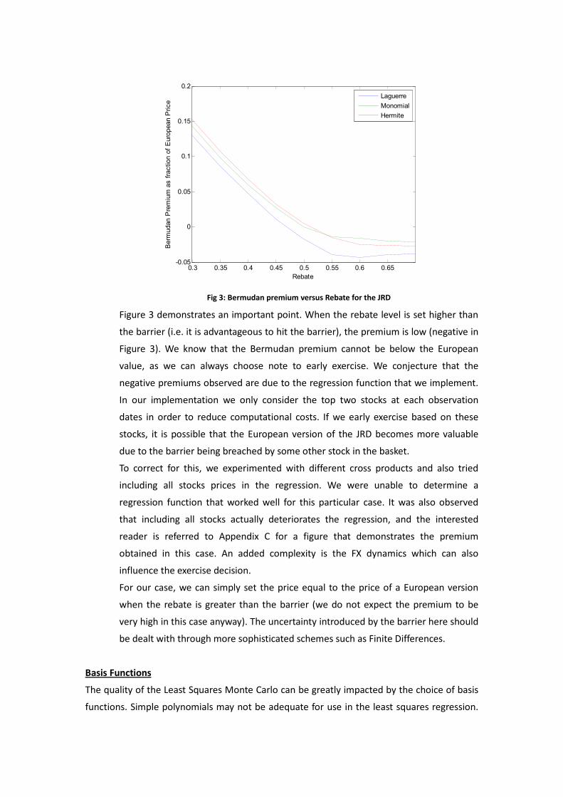
Fig 3: Bermudan premium versus Rebate for the JRD

Figure 3 demonstrates an important point. When the rebate level is set higher than

the barrier (i.e. it is advantageous to hit the barrier), the premium is low (negative in

Figure 3). We know that the Bermudan premium cannot be below the European

value, as we can always choose note to early exercise. We conjecture that the

negative premiums observed are due to the regression function that we implement.

In our implementation we only consider the top two stocks at each observation

dates in order to reduce computational costs. If we early exercise based on these

stocks, it is possible that the European version of the JRD becomes more valuable

due to the barrier being breached by some other stock in the basket.

To correct for this, we experimented with different cross products and also tried

including all stocks prices in the regression. We were unable to determine a

regression function that worked well for this particular case. It was also observed

that including all stocks actually deteriorates the regression, and the interested

reader is referred to Appendix C for a figure that demonstrates the premium

obtained in this case. An added complexity is the FX dynamics which can also

influence the exercise decision.

For our case, we can simply set the price equal to the price of a European version

when the rebate is greater than the barrier (we do not expect the premium to be

very high in this case anyway). The uncertainty introduced by the barrier here should

be dealt with through more sophisticated schemes such as Finite Differences.

Basis Functions

The quality of the Least Squares Monte Carlo can be greatly impacted by the choice of basis

functions. Simple polynomials may not be adequate for use in the least squares regression.

0.3 0.35 0.4 0.45 0.5 0.55 0.6 0.65-0.05

0

0.05

0.1

0.15

0.2

Rebate


Laguerre

Monomial

Hermite

We therefore experimented with a number of polynomials including Laguerre, Bessel

(varying orders), Chebyshev (1st and 2

nd kinds) and Hermite functions. Figure 4 shows the

rebate generated through different basis functions.

Fig 4: Bermudan premium versus number of basis functions for the JRD

For the JRD, we have a basket of 5 correlated stocks. So our choice of basis functions should

also allow for the correlation between these stocks. For computational economy we only

considered running regressions on the two best performing stocks and taking various cross

products of these stocks. A definition of the cross products can be found in Appendix B. We

found that the Chebyshev polynomials and the Bessel functions did not work well with a low

number of cross products (negative premiums generated). Figure 5 demonstrates the impact

of changing the number of cross products on Laguerre and Hermite polynomials.

Note that the “monomial” basis function was taken from [2], and we do not change the

number of cross products in this, therefore it is simply one value.

1 2 3 4 5 6 7-0.05

0

0.05

0.1

0.15

0.2

Number of Basis Functions


Laguerre

Monomial

Hermite

Chebyshev1st

Chebyshev2nd

Bessel

Fig 5: Bermudan premium versus number of cross products for the JRD

Another check on the use of different basis functions is to consider the impact of changing

the strike. We do not expect big differences in premiums depending on whether the JRD is in

the money or out of the money. Basis functions that describe this behavior are more suited

for pricing the JRD dynamically. Figure 6 shows premium for Laguerre, Monomials and

Hermite functions (the others do not produce valid results).

Fig 6: Bermudan premium versus normalized strike for the JRD

Figure 6 demonstrates that Monomials and Hermite functions produce the most consistent

results overall. In the pricing numbers presented in tables 3 and 4, we use 10 Hermite

polynomials.

1 2 3 4 5 6 7-0.02

0

0.02

0.04

0.06

0.08

0.1

0.12

0.14

0.16

0.18

Number of cross products


Laguerre

Monomial

Hermite

0.94 0.96 0.98 1 1.02 1.04 1.060.04

0.06

0.08

0.1

0.12

0.14

0.16

0.18

Normalized Strike


Laguerre

Monomial

Hermite

Hedging

In this section we present two techniques for hedging the JRD 1) Dynamic Hedging and 2)

Static Hedging. In dynamic hedging we simulate various trajectories for the underlying stocks,

and at each point compute the delta. Based on the delta we can form a replicating portfolio

that can hedge our short position in the product (assuming we sold the product). By contrast

static hedging assumes that we do not change our hedging portfolio over the lifetime of the

product. We therefore need to mimic the JRD’s early exercise and FX features, and we

achieve this by using a combination of barrier and quanto options.

Dynamic Delta Hedging

We follow a dynamic delta hedging strategy and compute the cost of hedging based on the

change in delta at each time step. This procedure is outlined in greater detail in Hull [3].

To test this strategy we first simulate a set of asset trajectories (without loss of generality we

assume the FX rate is fixed). We will test the delta hedging scheme as if these simulated

trajectories are out of sample realized prices. We choose to carry out the hedging using

Monte Carlo, and in particular using the CV approach. The other two alternatives (i.e.,

Likelihood Ratio and Pathwise Derivative) require us to compute partial derivatives, which is

outside the scope of our investigation.

Figure 7 shows some sample trajectories. Note that the prices here are the actual stock

prices from Appendix A (i.e not the normalized stock prices).

Fig 7: Bermudan premium versus number of cross products for the JRD

Starting from time zero and moving forward in time, we calculate the unperturbed derivative

price PF and five perturbed prices PG�,.,/,0,1. The unperturbed price is calculated simply by

using the MC pricing function with maturity and spot prices updated for each time step. For

0 2 4 6 8 10 12 14 16 180

50

100

150

200

250

300

350Sample Realized Trajectories

each of the perturbed prices, we change the corresponding spot price by multiplying it by �1 + ϵ" where ϵ is small. Note that in calculating the 6 prices (perturbed or unperturbed),

we have used the same set of Wiener processes for the Monte Carlo simulations. This

ensures that the error converges. The individual deltas are then approximated by taking the

ratio of

Δ� = PG� − PFϵPF , ∀i We rebalance the replicating portfolio one period later by changing our unit of stock holdings

to these one-period-lagged deltas. The rebalancing is self-financed by changing the position

in a USD, and in turn a JPY, cash account (recall that in this case the FX rate is fixed). By

repeating this procedure until knock-out or expiry, we obtained a cost (or profit) of hedging

in JPY. If the hedging has been effective, we would expect that the discounted cost should

equal the derivative price.

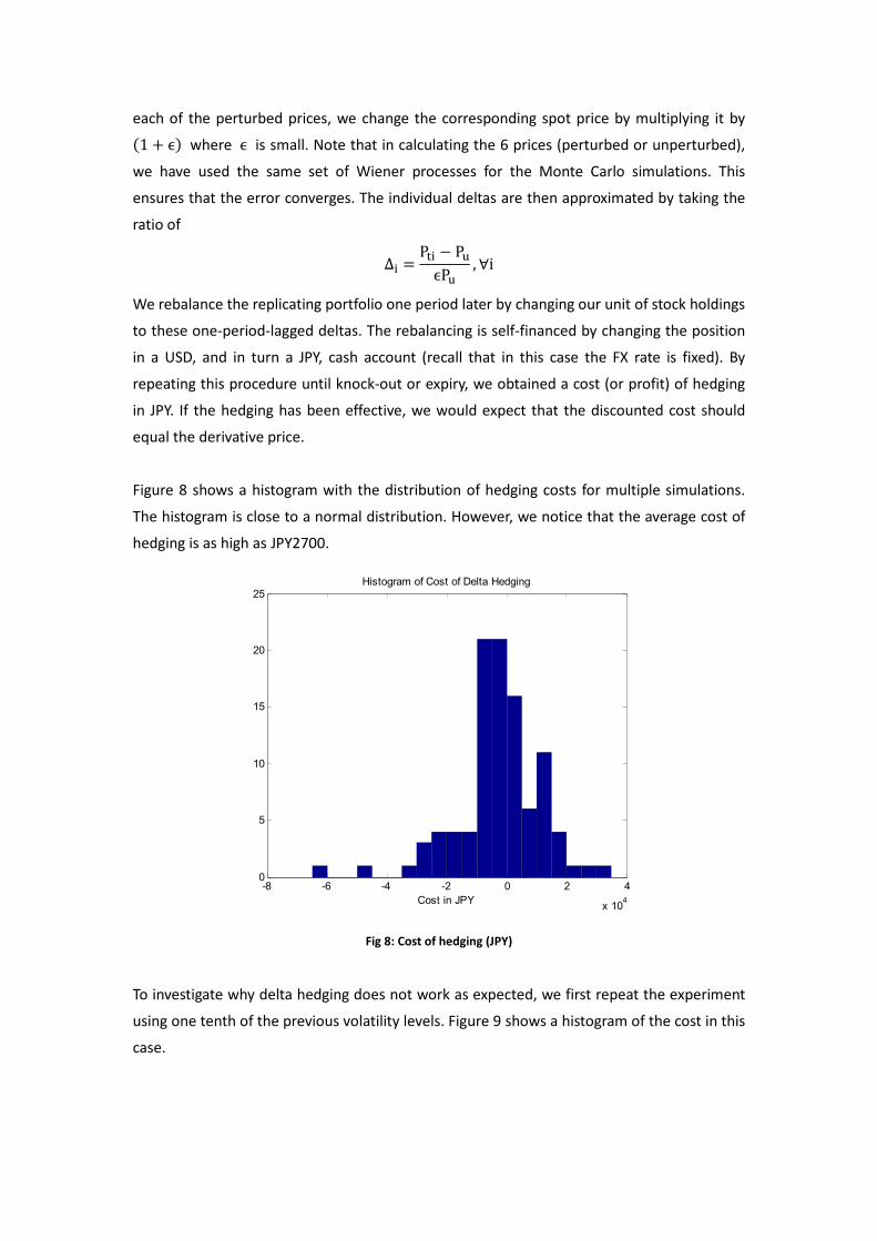
Figure 8 shows a histogram with the distribution of hedging costs for multiple simulations.

The histogram is close to a normal distribution. However, we notice that the average cost of

hedging is as high as JPY2700.

Fig 8: Cost of hedging (JPY)

To investigate why delta hedging does not work as expected, we first repeat the experiment

using one tenth of the previous volatility levels. Figure 9 shows a histogram of the cost in this

case.

-8 -6 -4 -2 0 2 4

x 104

0

5

10

15

20

25

Cost in JPY

Histogram of Cost of Delta Hedging

Fig 9: Cost of hedging (One Tenth volatility)

The average cost of hedging drops from JPY2700 to JPY800. Furthermore, if we look at the

change in the deltas in different time steps, as shown in the following table, the value of

delta can change abruptly at different points in time.

Time Step KL KM KN KO KP

1 0.0326 0.1617 0.7020 0.1110 3.7821

2 0.0348 0.1829 5.7690 3.7583 1.0930

3 0.0410 0.1817 0.4511 0.1464 -16.9050

4 0.0378 0.2077 1.4777 0.1937 1.4602

Table 5: Delta with respect to individual stocks

Taking the two pieces of evidence into account, we make the following postulation regarding

the poor performance of delta hedging for JRD. The payoff of JRD depends on the return of

the best performer in the basket. By this nature, the value of the JRD is a highly non-linear

function of the underlying asset prices. As a didactic example, suppose that by the CV

approach we perturb the price of Asset 1 and found that Δ� = 0.03 and suppose that at

this price level Asset 1 is the best performer. When the price of Asset 1 changes further,

however, it ceases to be the best performer and the JRD value is determined by the return of

Asset 4. As a consequence Δ� is not a smooth function of S1. This agrees with the abruptly

changing deltas we saw in the table. In other words, the gamma of JRD is so high that delta

hedging simply cannot capture the instantaneous risk. This also agrees with the fact that

under lower volatility the hedging performance is marginally improved, since under lower

volatility a best performer has a higher probability to remain the best performer, and vice

versa.

-1.5 -1 -0.5 0 0.5 1 1.5

x 104

0

5

10

15

20

25

Cost in JPY

Histogram of Cost of Delta Hedging

This analysis suggests that hedging may better be achieved through a static approach, where

we do not need to rebalance and incur hedging costs at each observation date. This is

discussed in the next section.

Static Hedging

The exotic features of this product include:

Rainbow option (best performance of the five underlying)

Exchange option (paid in JPY)

Knock out Barrier option (can be triggered by any of the five assets)

First touch option (rebate)

Due to the nature of complexity of the product, it is quite difficult to achieve perfect hedging

by implementing a static hedging strategy. Therefore, we employ an approximate static

hedging using Mean Monte Carlo (MMC). This procedure is equivalent to partially hedging

the claim using a portfolio of simpler assets. If the residual risk is deemed appropriate or can

be reduced to a suitable level, the static portfolio can be employed in place of complex

dynamic hedging procedures (for further details refer to Pellizzari 2001 [6]).

Here we denote the final payoff of the coupon at R = S as T� �U , .U … WU" . We then

choose a combination of low dimensional instruments {YU�Z"}\]�,.…W, ^ℎ`a` YU�Z" = T�b� �U", b� .U", … \U , … b� WU""

Such that the variance of

T� �U , .U … WU" − c d\YU�Z"W\]�

is minimized. However, the barrier in our product can be triggered by any asset. So it is quite

different from a combination of multiple barrier options each of which has a single

underlying asset with its own barriers.

As the base price is set at time 0, the strike prices for all the options are at the money. The

hedging portfolio then consists of:

Six month at the money European Barrier options on three of the most volatile underlying

stocks

Six month at the money European Exchange Option between USD and JPY

Six month European first touch options on three of the most volatile underlying stocks

The trading strategy is to hold the hedging portfolio at the beginning, with the weight

determined by the following procedure, and remaining money is put into a risk free account.

For each trajectory, if the product hit the barrier, we clear all of our positions, pay the rebate,

and put the remaining, if any left, into risk free account till the end. If the product is early

exercised, we clear all of our positions as well and pay the option payoff, and put the

remaining, if any left, into risk free account till the end. We took 10,000 trajectories and

recorded the payoff profit and loss for each one. We then chose our weight of holding on

each component such that the total variance of final profit and loss is minimized. Finally we

used the weights calculated above to test the hedging on another 10,000 trajectories. The

result is summarized in Table 6.

efgL% efgP% efgMP% ijklmnknmo

MMC Hedging -0.22627 -0. 13964 -0.014769 0.077624

Without Hedging -0.30433 -0.23425 -0.14161 0.15011

Table 6: Simulation results with MMC hedging

Fig 10: PnL with MMC hedging

Fig 11: PnL without MMC hedging (note the big positive premium and fat tail)

We can find that although the hedging portfolio is not completely hedged, the hedging

portfolio weighted by the Mean Monte Carlo technique using 10,000 simulations is better

distributed than the unhedged portfolio results as shown in Figures 10 and 11 (both VAR and

volatility are much smaller).

As the market marker, it would not be hard to get these instruments from the OTC market.

If we cannot find a barrier option with the desired barrier in the market, we can instead

replicate this single barrier option with a combination of vanilla index options with different

strikes, using the hedging techniques suggested by Carr and Chou [7].

It is clear that the static hedging appears to work better for the JRD, due to the hedging costs

involved with dynamic hedging. The dimensionality of the problem is the critical factor here.

With a high dimension product, we are faced with very high delta’s and this is difficult to

hedge with only first order hedging. If we have access to a market with other exotic options

on single assets, we can however create a hedging portfolio that minimizes our variance as

demonstrated by the MMC hedging technique.

Final Remarks

In this paper we have demonstrated pricing and hedging of a complicated structured product

using the Least Squares Monte Carlo approach. We saw that as the dimensionality of the

product increases, we are forced to think of innovative techniques to achieve the desired

accuracy from the pricing function. In this paper we achieved significant variance reduction

by using a combination of Sobol numbers and Brownian Bridges. To get comfortable with the

price of the product, we also benchmarked our pricing to several analytical results and a high

quality numerical result. We also demonstrated two different hedging techniques for this

product and showed that it is cheaper to use static hedging for the JRD note.

The MATLAB implementation of this product can be found in Appendix D for the interested

reader.

References

[1] Longstaff and Schwartz, “Valuing American options by simulation: a simple least-squares

approach”

[2] Tavella, Domingo A., Quantitative Methods in Derivatives Pricing

[3] Hull, John C., Options, Futures and Other Derivatives (6th

Edition)

[4] Johnson, Herb “Options on the Maximum or the Minimum of Several Assets.” The Journal

of Financial and Quantitative Analysis, Vol. 22, 1987

[5] Broadie and Glasserman

[6] Pellizzari, P. "Static Hedging of Multivariate Derivatives by Simulation." European Journal

of Operational Research (2005): 507-19. Web.

[7] Carr, Peter and Chou, Andrew “Breaking Barriers.” Risk September 1987

[8] Derman, E., D. Ergener, and I. Kani. Static Options Replication. Goldman, Sachs & Co.

[9] Jäckel, Peter. Monte Carlo Methods in Finance. Chichester, West Sussex, England: J. Wiley,

2002. Print.

[10] Piterbarg, V. “A Multi-currency Model with FX Volatility Skew.” (February 7, 2005).

Available at SSRN: http://ssrn.com/abstract=685084

[11] Pricing Power Reverse Dual Currency Notes. Available at

http://www.fincad.com/derivatives-resources/articles/price-power-reverse-dual-curr

ency.aspx

Appendix A – Parameters Used

The parameters used to price our final product:

Stocks used: Apple, Citi, P&G, American Express and Microsoft

Correlation Matrix:

1.0000 0.2957 0.3729 0.1930 0.2438 0

0.2957 1.0000 0.3819 0.3738 0.5604 0

0.3729 0.3819 1.0000 0.2846 0.3097 0

0.1930 0.3738 0.2846 1.0000 0.2846 0

0.2438 0.5604 0.3097 0.2846 1.0000 0

0 0 0 0 0 1

(note the final row and column refers to the FX rate, which is assumed to be uncorrelated

with the underlying stocks)

Volatilities: [0.15;0.2;0.23;0.3;0.1];

Spot Prices: [250;40;23;60;3.8];

Dividend Yields: [0.05;0.02;0.09;0.01;0.02];

Barriers: spots*1.2 (20% increase in any stock)

Rebate: 30%

Maturity: 1 year

Coupon maturity : 1 year (annual)

Foreign Interest Rates: 5%

Domestic Interest Rates: 1%

FX volatility: 15%

Initial FX Rate: 100

Appendix B – Basis Functions and Cross Products

Laguerre Polynomials

1 1

2 − + 1

3 12 �. − 4 + 2"

4 16 �−/ + 9. − 18 + 6"

5 124 �0 − 16/ + 72. − 96 + 24"

6 1120 �−1 + 250 − 200/ + 600. − 600 + 120"

7 1720 �v − 361 + 4500 − 2400/ + 5400. − 4320 + 720"

Hermite (probabilists) Polynomials

1 1

2

3 . − 1

4 / − 3

5 0 − 6. + 3

6 1 − 10/ + 15

7 v − 150 + 45. − 15

8 w − 211 − 105/ + 105

9 x − 28v + 2100 − 420. + 105

10 y − 36w + 3781 − 1260/ + 945

Chebyshev (1st kind) Polynomials

1 1

2

3 2. − 1

4 4/ − 3

5 80 − 8. + 1

6 161 − 20/ + 5

7 32v − 480 + 18. − 1

8 64w − 1121 + 56/ − 7

9 128x − 256v + 1600 − 32. + 1

10 256y − 576w + 4321 − 120/ + 9

Chebyshev (2nd

kind) Polynomials

1 1

2 2

3 4. − 1

4 8/ − 4

5 160 − 12. + 1

6 321 − 32/ + 6

7 64v − 800 + 24. − 1

8 128w − 1921 + 80/ − 8

9 256x − 448v + 2400 − 40. + 1

10 512y − 1024w + 6721 − 160/ + 10

Bessel Functions: We use the MATLAB implementation of the Bessel functions of various

orders

Monomials (taken from Tavella[2])

1 � + �. + �/ + �0 + �1

2 . + .. + ./ + .0 + .1

3 � . + � .. + � ./ + � .0

4 �. . + �. .. + �. ./

5 �/ . + �/ ..

6 �0 .

7 1

For the basis functions (Laguerre, Hermite and Laguerre), we use the following cross

products:

1 �

2 .

3 � .

4 �. .

5 �/ .

6 �. ..

7 �/ ./

We also tried cross products with all 5 stocks included

1 �.

2 ..

3 /.

4 0.

5 1.

6 � .

7 �. .

8 � /

9 � 0

10 � 1

11 . /

12 . 0

Appendix C – Misc Graphs

Fig C.1: Bermudan premium with varying div yields

From Fig C.1 it is clear that the Chebyshev polynomials and Bessel functions do not work well

with low dividend yields and generate negative premiums.

Fig C.2: Bermudan premium with varying rebates

Fig C.2 shows that Chebyshev polynomials and Bessel functions do not work well with

barriers. In the paper we talked about how we obtained negative premiums even with

Hermite, laguerre and monomials when the rebate was set high above the barrier. We

hypothesized that this was due to the other components of the basket which were not

0 0.02 0.04 0.06 0.08 0.1 0.12 0.14 0.16 0.18 0.2-0.5

-0.4

-0.3

-0.2

-0.1

0

0.1

0.2

0.3

Div Yield


Chebyshev1st

Chebyshev2nd

Bessel

0.3 0.35 0.4 0.45 0.5 0.55 0.6 0.65-0.8

-0.7

-0.6

-0.5

-0.4

-0.3

-0.2

-0.1

0

0.1

Rebate


Chebyshev1st

Chebyshev2nd

Bessel

Hermite with all cross products

included in the least squares regression. However Fig C.2 shows that even when we include

more cross products which cover all the assets, we obtain negative premiums. In fact in this

case the regression does not work well at all, with consistent negative premiums. This

suggests that either the basis functions and cross products need to be more complex, or that

the LSMC technique cannot handle the complexity introduced by the barriers and the

dimensionality of the product, and we must use other schemes such as Finite Differencing.

Fig C.3: Bermudan premium with varying rebates

Fig C.3 shows the Bermudan premium against normalized strikes when using Chebyshev and

Bessel functions. Bessel functions do produce a positive premium, but the premium is much

lower than we expect. We therefore disregard these functions.

0.94 0.96 0.98 1 1.02 1.04 1.06-0.35

-0.3

-0.25

-0.2

-0.15

-0.1

-0.05

0

0.05

0.1

Normalized Strike


Chebyshev1st

Chebyshev2nd

Bessel

Appendix D – MATLAB implementation

%%%%%%%%%%%%%%%%%%%%%%%%%%%%%%%%%%%%%%%%%%%%%%%%%%%%%%%%

% Main pricing function (includes all variance reduction

% techniques and also prices the European version)

%%%%%%%%%%%%%%%%%%%%%%%%%%%%%%%%%%%%%%%%%%%%%%%%%%%%%%%%

function MCResults=jrd_LSMC(maturity, vols, divYields, foreignRate,...

spots, strikes,observation_frequency, cycles, corMatrix,

basketSize,extraAssets, ...

highBarrier,rebate,domesticRate,fxVol,fxRate,batches,MCType,useBrowni

anBridge,...

basisType,basisFns,crossProducts,productType)

MCResults=zeros(3,1);

% parameters

interval = 1/observation_frequency;

payoffs = zeros(batches,1);

cholMatrix=chol(corMatrix)';

strikes = strikes./spots; %scale strike for ease of use in basis functions

time_steps = observation_frequency*maturity + 1;

dimensions=(basketSize + extraAssets + 1)*(time_steps-1);

highBarrier= highBarrier./spots;

if strcmp(MCType,'sobol')

sobol_obj=sobolset(dimensions,'Skip',1e3);

end

for i=1:batches


sobol_seq=sobol_obj((i-1)*cycles+1:i*cycles,:);

sobol_norm=norminv(sobol_seq);

sobol_norm_seq=reshape(sobol_norm,[cycles,time_steps-1,

basketSize + extraAssets + 1]);

elseif strcmp(MCType,'lhs')

lhs_unformatted=lhsdesign(cycles,dimensions,'smooth','off','criterion

','correlation');

lhs_unformatted=norminv(lhs_unformatted);

lhs=reshape(lhs_unformatted,cycles,time_steps-1,basketSize +

extraAssets + 1);

end

% work with normalizes stock prices and fx rates, hence period 0 values

% are 1

trajectories = ones(cycles, time_steps, basketSize + extraAssets);

fxTrajectories = ones(cycles,time_steps);

trajectoriesW = ones(cycles, time_steps, basketSize + extraAssets);

fxTrajectoriesW = ones(cycles,time_steps);

% generate weiner processes

if useBrownianBridge % steps must be in 2^k + 1 format!

currInterval = maturity;

% generate beginning and end points

randSetIndex = 1;

beginW = zeros(cycles,basketSize + extraAssets);

beginFxW = zeros(cycles,1);

trajectoriesW(:,1,:) = reshape(beginW,cycles,1,basketSize +

extraAssets);

fxTrajectoriesW(:,1) = beginFxW;


endW =

(cholMatrix*sobol_norm(:,randSetIndex:randSetIndex+basketSize+extraAs

sets-1)')'*sqrt(currInterval);

randSetIndex = randSetIndex + basketSize+extraAssets;

endFxW =

sobol_norm(:,randSetIndex:randSetIndex)*sqrt(currInterval);

randSetIndex = randSetIndex + 1;


endW =

(cholMatrix*lhs_unformatted(:,randSetIndex:randSetIndex+basketSize+ex

traAssets-1)')'*sqrt(currInterval);


endFxW =

lhs_unformatted(:,randSetIndex:randSetIndex)*sqrt(currInterval);


end

trajectoriesW(:,time_steps,:) =

reshape(endW,cycles,1,basketSize + extraAssets);

fxTrajectoriesW(:,time_steps) = endFxW;

bbInterval = interval;

while (currInterval > interval)

bbIndex = 1;

trajIndex = 1;

while (bbIndex*currInterval <= maturity)


currZ =

(cholMatrix*sobol_norm(:,randSetIndex:randSetIndex+basketSize+extraAs

sets-1)')';


currFxZ = sobol_norm(:,randSetIndex:randSetIndex);



currZ =

(cholMatrix*lhs_unformatted(:,randSetIndex:randSetIndex+basketSize+ex

traAssets-1)')';


currFxZ =

lhs_unformatted(:,randSetIndex:randSetIndex);


end

variance = currInterval/4;

currW = 0.5*(beginW+endW) + sqrt(variance)*currZ;

currFxW = 0.5*(beginFxW+endFxW) + sqrt(variance)*currFxZ;

trajIndex = trajIndex +

((time_steps-1)/(maturity/(currInterval/2)));

trajectoriesW(:,trajIndex,:) =

reshape(currW,cycles,1,basketSize + extraAssets);

fxTrajectoriesW(:,trajIndex) = currFxW;

bbIndex = bbIndex + 1;

beginW = endW; beginFxW = endFxW;

trajIndex = trajIndex +

((time_steps-1)/(maturity/(currInterval/2)));

endIndex =

((time_steps-1)/(maturity/currInterval))*bbIndex + 1;

if endIndex <= time_steps

endW =

reshape(trajectoriesW(:,endIndex,:),cycles,basketSize + extraAssets);

endFxW = fxTrajectoriesW(:,endIndex);

end

end

currInterval = currInterval/2;

beginW = zeros(cycles,basketSize + extraAssets);

beginFxW = zeros(cycles,1);

trajIndex = ((time_steps-1)/(maturity/currInterval)) + 1;

endW =

reshape(trajectoriesW(:,trajIndex,:),cycles,basketSize + extraAssets);

endFxW = fxTrajectoriesW(:,trajIndex);

bbInterval = bbInterval/2;

end

% free memory

clear beginW endW beginFxW endFxW currW currFxW;

% generate trajectories

for j=2:time_steps

for k=1:basketSize + extraAssets

trajectories(:,j,k) =

trajectories(:,j-1,k).*exp((foreignRate...

-divYields(k)-0.5*(vols(k)^2))*interval +

vols(k)*(trajectoriesW(:,j,k)-trajectoriesW(:,j-1,k)));

end

fxTrajectories(:,j) =

fxTrajectories(:,j-1).*exp((domesticRate...

-foreignRate-0.5*(fxVol^2))*interval +

fxVol*(fxTrajectoriesW(:,j)-fxTrajectoriesW(:,j-1)));

end

clear trajectoriesW fxTrajectoriesW;

else

for j=2:time_steps


sobol_eachtimeStep=reshape(sobol_norm_seq(:,(j-1),:),[cycles,


z=sobol_eachtimeStep(:,1:basketSize +

extraAssets)*cholMatrix';

fxZ=sobol_eachtimeStep(:,basketSize + extraAssets +

1:basketSize + extraAssets + 1);


lhs_eachtimeStep=reshape(lhs(:,(j-1),:),[cycles,


z=lhs_eachtimeStep(:,1:basketSize +

extraAssets)*cholMatrix';

fxZ=lhs_eachtimeStep(:,basketSize + extraAssets +

1:basketSize + extraAssets + 1);

else

z=(cholMatrix*normrnd(0,1,basketSize +

extraAssets,cycles))';

fxZ=randn(cycles,1);

end






vols(k)*sqrt(interval)*z(:,k));

end




fxVol*sqrt(interval)*fxZ);

end

end

clear z sobol_norm_seq sobol_norm lhs_unformatted lhs; % free up memory

% work backwards

cfMatrix = zeros(cycles, time_steps-1);

cfMatrixPlusRebate= zeros(cycles, observation_frequency*maturity);

stillAlive=zeros(cycles, observation_frequency*maturity);

% determine final payoff based on initial composition of the basket

currPrice = reshape(trajectories(:,time_steps,1:basketSize),cycles,

basketSize);

cfMatrix(:,time_steps-1) = (max(max(currPrice...

-

repmat(strikes(1:basketSize)',cycles,1),0),[],2)).*fxTrajectories(:,t

ime_steps-1);

alive=ones(cycles,1);

% determine the trajectories where the barriers are not breached

for m=1:observation_frequency*maturity

temp=reshape(trajectories(:,m+1,:),cycles,basketSize);

alive=alive.* min((repmat(highBarrier',cycles,1)-temp)>0,[],2);

stillAlive(:,m)=alive;

end

breachingPoint=[ones(cycles,1),stillAlive(:,1:(end-1))]-

stillAlive;

cfMatrix(:,time_steps-1)=cfMatrix(:,time_steps-1).*stillAlive(:,time_

steps-1);

% pay rebate at the point where barriers were breached

cfMatrixPlusRebate = cfMatrix + rebate.*breachingPoint;

% loop through to determine bermudan value

if strcmp(productType,'bermudan')

for j=time_steps-1:-1:1

% determining current exercise value

currPrice = reshape(trajectories(:,j+1,1:basketSize),cycles,

basketSize);

exerciseCF = (max(max(currPrice -

repmat(strikes(1:basketSize)',cycles,1),0),[],2)).*fxTrajectories(:,j

+1);

exerciseCF = exerciseCF.*stillAlive(:,j); % cannot exercise if

knocked out

moneyness = exerciseCF>0;

pvVector = zeros(cycles,1);

for k=j+1:time_steps-1

% As all future cashflows have already been converted to

% the

% domestic currency discounting done in domestic rate

pvVector = pvVector +

cfMatrixPlusRebate(:,k)*exp(-domesticRate*interval*(k-j));

end

% only consider the two best performing assets for the least

% squares regression

sortedPrices =

reshape(sort(trajectories(:,j+1,1:basketSize),3,'descend'),cycles,bas

ketSize);

currPrices = sortedPrices(:,1:2);

if sum(moneyness)==0

condExpect = moneyness;

else

if strcmp(basisType,'all')

condExpect =

LSR(sortedPrices,pvVector,basisType,basisFns,crossProducts,moneyness)

else

condExpect =

LSR(currPrices,pvVector,basisType,basisFns,crossProducts,moneyness);

end

end

cfMatrix(:,j) = moneyness.*((condExpect <

exerciseCF).*exerciseCF);

% If knocked out pay the rebate

cfMatrixPlusRebate(:,j) = cfMatrix(:,j) +

rebate*breachingPoint(:,j);

% set CF's of j+1 to maturity zero if exercised at current time

for k=j+1:time_steps-1

% If not exercised and not knocked out, keep old cashflows

cfMatrix(:,k) = cfMatrix(:,k).*(cfMatrix(:,j)==0);

cfMatrixPlusRebate(:,k) =

cfMatrixPlusRebate(:,k).*(cfMatrix(:,j)==0);

end

end

end

% Discount the CFs from the CF matrix to get option value

currPayoffs = zeros(cycles,1);

for j=time_steps-1:-1:1

currPayoffs = currPayoffs +

cfMatrixPlusRebate(:,j).*exp(-(domesticRate/observation_frequency)*j)

;

end

payoffs(i) = mean(currPayoffs)*fxRate; % Scale by current fxRate

end

clear trajectories fxTrajectories; % free memory

MCResults(1)=payoffs(1);

MCResults(2) = std(payoffs);

end

%%%%%%%%%%%%%%%%%%%%%%%%%%%%%%%%%%%%%%%%%%%%%%%%%%%%%%%%

% Function to perform Least Squares Regression for LSMC

%%%%%%%%%%%%%%%%%%%%%%%%%%%%%%%%%%%%%%%%%%%%%%%%%%%%%%%%

function condCF=LSR(currPrices, pvVector, fnType,

numFns,crossProducts,moneyness)

condCF=zeros(size(currPrices,1),1);

crossTerms = zeros(size(currPrices,1),7);

regressFns = numFns;

if strcmp(fnType,'simplest')

basisFns = zeros(size(currPrices,1),numFns);

for i=2:numFns

basisFns(:,i) = currPrices.^(i-1);

end

elseif strcmp(fnType,'sine')


for i=2:numFns

basisFns(:,i) = sin((i-1)*currPrices);

end

elseif strcmp(fnType,'monomial')


basisFns(:,1) = currPrices(:,1) + currPrices(:,1).^2 +

currPrices(:,1).^3 ...

+ currPrices(:,1).^4 + currPrices(:,1).^5;

if numFns >= 2

basisFns(:,2) = currPrices(:,2) + currPrices(:,2).^2 +


+ currPrices(:,2).^4 + currPrices(:,2).^5;

end

if numFns >= 3

basisFns(:,3) = currPrices(:,1).*currPrices(:,2) +

currPrices(:,1).*(currPrices(:,2).^2) ...

+ currPrices(:,1).*(currPrices(:,2).^3) +

currPrices(:,1).*(currPrices(:,2).^4);

end

if numFns >= 4

basisFns(:,4) = (currPrices(:,1).^2).*currPrices(:,2) +

(currPrices(:,1).^2).*(currPrices(:,2).^2) ...

+ (currPrices(:,1).^2).*(currPrices(:,2).^3);

end

if numFns >= 5

basisFns(:,5) = (currPrices(:,1).^3).*currPrices(:,2) +

(currPrices(:,1).^3).*(currPrices(:,2).^2);

end

if numFns >= 6

basisFns(:,6) = (currPrices(:,1).^4).*currPrices(:,2);

end

if numFns >= 7

basisFns(:,7) = 1;

end

elseif strcmp(fnType,'laguerre')

crossTerms(:,1) = sum(laguerre(currPrices(:,1),numFns),2);

crossTerms(:,2) = sum(laguerre(currPrices(:,2),numFns),2);

crossTerms(:,3) =

sum(laguerre(currPrices(:,1).*currPrices(:,2),numFns),2);

crossTerms(:,4) =

sum(laguerre((currPrices(:,1).^2).*currPrices(:,2),numFns),2);

crossTerms(:,5) =

sum(laguerre((currPrices(:,1).^3).*currPrices(:,2),numFns),2);

crossTerms(:,6) =

sum(laguerre((currPrices(:,1).^2).*(currPrices(:,2).^2),numFns),2);

crossTerms(:,7) =

sum(laguerre((currPrices(:,1).^3).*(currPrices(:,2).^3),numFns),2);

basisFns = crossTerms(:,1:crossProducts);

regressFns = crossProducts;

elseif strcmp(fnType,'Chebyshev1st')

crossTerms(:,1) = sum(Chebyshev1st(currPrices(:,1),numFns),2);

crossTerms(:,2) = sum(Chebyshev1st(currPrices(:,2),numFns),2);

crossTerms(:,3) =

sum(Chebyshev1st(currPrices(:,1).*currPrices(:,2),numFns),2);

crossTerms(:,4) =

sum(Chebyshev1st((currPrices(:,1).^2).*currPrices(:,2),numFns),2);

crossTerms(:,5) =

sum(Chebyshev1st((currPrices(:,1).^3).*currPrices(:,2),numFns),2);

crossTerms(:,6) =

sum(Chebyshev1st((currPrices(:,1).^2).*(currPrices(:,2).^2),numFns),2

);

crossTerms(:,7) =

sum(Chebyshev1st((currPrices(:,1).^3).*(currPrices(:,2).^3),numFns),2

);



elseif strcmp(fnType,'Chebyshev2nd')

crossTerms(:,1) = sum(Chebyshev2nd(currPrices(:,1),numFns),2);

crossTerms(:,2) = sum(Chebyshev2nd(currPrices(:,2),numFns),2);

crossTerms(:,3) =

sum(Chebyshev2nd(currPrices(:,1).*currPrices(:,2),numFns),2);

crossTerms(:,4) =

sum(Chebyshev2nd((currPrices(:,1).^2).*currPrices(:,2),numFns),2);

crossTerms(:,5) =

sum(Chebyshev2nd((currPrices(:,1).^3).*currPrices(:,2),numFns),2);

crossTerms(:,6) =

sum(Chebyshev2nd((currPrices(:,1).^2).*(currPrices(:,2).^2),numFns),2

);

crossTerms(:,7) =

sum(Chebyshev2nd((currPrices(:,1).^3).*(currPrices(:,2).^3),numFns),2

);



elseif strcmp(fnType,'Hermite')

crossTerms(:,1) = sum(Hermite(currPrices(:,1),numFns),2);

crossTerms(:,2) = sum(Hermite(currPrices(:,2),numFns),2);

crossTerms(:,3) =

sum(Hermite(currPrices(:,1).*currPrices(:,2),numFns),2);

crossTerms(:,4) =

sum(Hermite((currPrices(:,1).^2).*currPrices(:,2),numFns),2);

crossTerms(:,5) =


crossTerms(:,6) =

sum(Hermite((currPrices(:,1).^2).*(currPrices(:,2).^2),numFns),2);

crossTerms(:,7) =

sum(Hermite((currPrices(:,1).^3).*(currPrices(:,2).^3),numFns),2);



elseif strcmp(fnType,'all')

crossTerms(:,1) = sum(Hermite(currPrices(:,1).^2,numFns),2);





crossTerms(:,6) =


crossTerms(:,7) =


crossTerms(:,8) =


crossTerms(:,9) =


crossTerms(:,10) =


crossTerms(:,11) =


crossTerms(:,12) =

sum(Hermite(currPrices(:,1).*currPrices(:,2),numFns),2)...

+sum(Hermite(currPrices(:,2).*currPrices(:,3),numFns),2);


regressFns = 12;

elseif strcmp(fnType,'bessel')

crossTerms(:,1) = sum(bessel(numFns,currPrices(:,1)),2);

crossTerms(:,2) = sum(bessel(numFns,currPrices(:,2)),2);

crossTerms(:,3) =

sum(bessel(numFns,currPrices(:,1).*currPrices(:,2)),2);

crossTerms(:,4) =

sum(bessel(numFns,(currPrices(:,1).^2).*currPrices(:,2)),2);

crossTerms(:,5) =

sum(bessel(numFns,(currPrices(:,1).^3).*currPrices(:,2)),2);

crossTerms(:,6) =

sum(bessel(numFns,(currPrices(:,1).^2).*(currPrices(:,2).^2)),2);

crossTerms(:,7) =

sum(bessel(numFns,(currPrices(:,1).^3).*(currPrices(:,2).^3)),2);



end

% basisFns(:,1) = basisFns(:,1).*moneyness;

formattedBasisFns = zeros(sum(moneyness),regressFns);

formattedPvs = zeros(sum(moneyness),1);

counter = 1;

for i=1:size(currPrices,1)

if moneyness(i)==1

formattedBasisFns(counter,:) = basisFns(i,:);

formattedPvs(counter,:) = pvVector(i,:);

counter = counter + 1;

end

end

b = regress(formattedPvs,formattedBasisFns);

if strcmp(fnType,'simplest')

for i=1:numFns

condCF = condCF + b(i)*currPrices.^(i-1);

end

elseif strcmp(fnType,'sine')

condCF = b(1);

for i=2:numFns

condCF = condCF + b(i)*sin((i-1)*currPrices);

end

elseif strcmp(fnType,'monomial')

condCF = condCF + b(1)*(currPrices(:,1) + currPrices(:,1).^2 +


+ currPrices(:,1).^4 + currPrices(:,1).^5);

if numFns >= 2

condCF = condCF + b(2)*(currPrices(:,2) + currPrices(:,2).^2 +


+ currPrices(:,2).^4 + currPrices(:,2).^5);

end

if numFns >= 3

condCF = condCF + b(3)*(currPrices(:,1).*currPrices(:,2) +

currPrices(:,1).*(currPrices(:,2).^2) ...

+ currPrices(:,1).*(currPrices(:,2).^3) +

currPrices(:,1).*(currPrices(:,2).^4));

end

if numFns >= 4

condCF = condCF + b(4)*((currPrices(:,1).^2).*currPrices(:,2) +

(currPrices(:,1).^2).*(currPrices(:,2).^2) ...

+ (currPrices(:,1).^2).*(currPrices(:,2).^3));

end

if numFns >= 5

condCF = condCF + b(5)*((currPrices(:,1).^3).*currPrices(:,2) +

(currPrices(:,1).^3).*(currPrices(:,2).^2));

end

if numFns >= 6

condCF = condCF + b(6)*((currPrices(:,1).^4).*currPrices(:,2));

end

if numFns >= 7

condCF = condCF + b(7);

end

elseif strcmp(fnType,'all')

condCF = condCF + b(1)*sum(Hermite(currPrices(:,1).^2,numFns),2);





condCF = condCF +

b(6)*sum(Hermite(currPrices(:,1).*currPrices(:,2),numFns),2);

condCF = condCF +

b(7)*sum(Hermite((currPrices(:,1).^2).*currPrices(:,2),numFns),2);

condCF = condCF +


condCF = condCF +


condCF = condCF +


condCF = condCF +


condCF = condCF +

b(12)*sum(Hermite(currPrices(:,1).*currPrices(:,2),numFns),2)...

+sum(Hermite(currPrices(:,2).*currPrices(:,3),numFns),2);

else

condCF = condCF + b(1)*crossTerms(:,1);

if crossProducts >= 2


end



end



end



end



end



end

end

condCF = condCF.*moneyness;

end

function out=laguerre(x, n)

y0=ones(size(x,1),1);

y1=-x+1;

y2=0.5*(x.^2-4*x+2);

y3=(1/6)*(-x.^3+9*x.^2-18*x+6);

y4=(1/24)*(x.^4-16*x.^3+72*x.^2-96*x+24);

y5=(1/120)*(-x.^5+25*x.^4-200*x.^3+600*x.^2-600*x+120);

y6=(1/720)*(x.^6-36*x.^5+450*x.^4-2400*x.^3+5400*x.^2-4320*x+720);

Y=[y0 y1 y2 y3 y4 y5 y6];

out=Y(:,1:n);

end

function out=Chebyshev1st(x, n)


y1=x;

y2=2*x.^2-1;

y3=4*x.^3-3*x;

y4=8*x.^4-8*x.^2+1;

y5=16*x.^5-20*x.^3+5*x;

y6=32*x.^6-48*x.^4+18*x.^2-1;

y7=64*x.^7-112*x.^5+56*x.^3-7*x;

y8=128*x.^8-256*x.^6+160*x.^4-32*x.^2+1;

y9=256*x.^9-576*x.^7+432*x.^5-120*x.^3+9*x;

Y=[y0 y1 y2 y3 y4 y5 y6 y7 y8 y9];

out=Y(:,1:n);

end

function out=Chebyshev2nd(x, n)


y1=2*x;

y2=4*x.^2-1;

y3=8*x.^3-4*x;

y4=16*x.^4-12*x.^2+1;

y5=32*x.^5-32*x.^3+6*x;

y6=64*x.^6-80*x.^4+24*x.^2-1;

y7=128*x.^7-192*x.^5+80*x.^3-8*x;

y8=256*x.^8-448*x.^6+240*x.^4-40*x.^2+1;

y9=512*x.^9-1024*x.^7+672*x.^5-160*x.^3+10*x;

Y=[y0 y1 y2 y3 y4 y5 y6 y7 y8 y9];

out=Y(:,1:n);

end

function out=Hermite(x, n)


y1=x;

y2=x.^2-1;

y3=x.^3-3*x;

y4=x.^4-6*x.^2+3;

y5=x.^5-10*x.^3+15*x;

y6=x.^6-15*x.^4+45*x.^2-15;

y7=x.^7-21*x.^5+105*x.^3-105*x;

y8=x.^8-28*x.^6+210*x.^4-420*x.^2+105;

y9=x.^9-36*x.^7+378*x.^5-1260*x.^3+945*x;

Y=[y0 y1 y2 y3 y4 y5 y6 y7 y8 y9];

out=Y(:,1:n);

end

%%%%%%%%%%%%%%%%%%%%%%%%%%%%%%%%%%%%%%%%%%%%%%%%%%%%%%%%

% Code for dynamic delta

%%%%%%%%%%%%%%%%%%%%%%%%%%%%%%%%%%%%%%%%%%%%%%%%%%%%%%%%

clc;

clear;

format short g;

warning('off', 'stats:regress:RankDefDesignMat');

corMatrix= [1.0000, 0.2957, 0.3729, 0.1930, 0.2438;

0.2957, 1.0000, 0.3819, 0.3738, 0.5604;

0.3729, 0.3819, 1.0000, 0.2846, 0.3097;

0.1930, 0.3738, 0.2846, 1.0000, 0.2846;

0.2438, 0.5604, 0.3097, 0.2846, 1.0000];

corMatrix = eye(1);

vols=[.15;.2;.23;0.3;0.1];

divYields=[0.1;0.1;0.1;0.1;0.1];

spots=[250;40;23;60;3.8];

strikes=[250;40;23;60;3.8];

barriers=spots*1.2;

cycles = 1000;

size = 1;

foreignRate = 0.05;

obsFreq = 16;

basketSize = 5;

extraAssets = 0;

rebate = 0.3;

domesticRate = 0.01;

fxVol = 0.15;

fxRate = 100;

maturity = 1;

batches = 1;

basisType = 'Hermite';

basisFns = 10;

crossProducts = 3;

dimensions=(basketSize + extraAssets + 1)*(obsFreq*maturity);

useBrownianBridge = 1;

productType = 'bermudan';

% parameters

interval = 1/obsFreq;

payoffs = zeros(batches,1);


time_steps = obsFreq*maturity + 1;

dimensions=(basketSize + extraAssets + 1)*(time_steps-1);

pertDS = 0.0001; %this is the percentage perturbation in the underlying

asset

dummy = 0;

batches_hedge = 100;

termValues = [];

cumcostYen_dump=zeros(batches_hedge,time_steps-1);der_price=zeros(bat

ches_hedge,time_steps-1);

num_TotIntervals = time_steps; %number of total intevals over the entire

maturity

for q = 1:batches_hedge

currentPort= zeros(1,basketSize+extraAssets+2);

%generate the realized trajectories to carry out the hedging simulation

realTraj=(gen_traj(maturity, time_steps-1,corMatrix, vols,...

fxVol, spots,fxRate, divYields,

domesticRate,foreignRate,num_TotIntervals))';

cumcostYen = 0; %the cumulative cost in Japanese yen

dummy = 0; %dummy variable indicates if the barrier has been breached

for i = 1:time_steps-1

if i~=1

costYen=0;

cumcostYen=cumcostYen*exp(domesticRate*1/obsFreq);

%interest accrual in JPY

currentPort(1,end-1:end)=[currentPort(1,end-1)*exp(foreignRate*1/obsF

req),...

currentPort(1,end)*exp(domesticRate*1/obsFreq)]; %interest

accrual in USD

oldMMUSD = currentPort(1,6); %the USD money market account

prior to delta hedging

%if barrier is breached cash out the position

if max(realTraj(i,1:5))>barriers

terminalValue =

(currentPort(1,1:end-2)*realTraj(i,1:end-1)'...

+currentPort(1,end-1))*realTraj(i,end)+currentPort(1,end);

dummy = 1;

end

oldStockUSD=currentPort(1:end-2)*realTraj(i,1:end-1)';

%the USD value of the stocks

currentPort(1:end-2) = delta; %update the current portfolio

holding to delta

newStockUSD=currentPort(1:end-2)*realTraj(i,1:end-1)'; %new

portfolio holdings

currentPort(1,6)=currentPort(1,6)+(oldStockUSD-newStockUSD); %update

the USD money market

newMMUSD = currentPort(1,6); %update the USD money market

account after delta hedging

currentPort(1,7)=currentPort(1,7)+(oldMMUSD -

newMMUSD)*realTraj(i,end); %convert USD money market to JPY

costYen=(oldMMUSD - newMMUSD)*realTraj(i,end); %record the

current cost of hedging in JPY

cumcostYen=cumcostYen+costYen; %update the cumulative cost in

JPY

cumcostYen_dump(q,i-1)=cumcostYen; %store the values of the

cumcostYen

end

if dummy ~= 1

norm_spots=realTraj(i,1:5)./realTraj(i,1:5); %normalize the

spots to 1

%select the price at time step i and replicate

trajectories = repmat(norm_spots,cycles,1);

fxTrajectories = ones(cycles,time_steps);

%reshape the 2D matrix into a 3D matrix

temp =

reshape(trajectories,cycles,1,basketSize+extraAssets);

trajectories=zeros(cycles, time_steps+1-i, basketSize +

extraAssets);

trajectoriesP=zeros(cycles, time_steps+1-i, basketSize +

extraAssets);

trajectories(:,1,:) = temp;

%create a matrix to store the brownian motions to use the same

%brownian motion for the perturbed and unperturbed trajectories

zMat =zeros(cycles, time_steps-i, basketSize + extraAssets);

fxZMat =zeros(cycles, time_steps-i);

for p=1:time_steps-i

zslice=(cholMatrix*normrnd(0,1,basketSize +

extraAssets,cycles))';

zslice=reshape(zslice,[cycles,1,basketSize +

extraAssets]);

zMat(:,p,:)=zslice;

fxZ=randn(cycles,time_steps-i);

end

for j=2:time_steps-i+1

% generate unperturbed trajectories





vols(k)*sqrt(interval)*zMat(:,j-1,k));

end




fxVol*sqrt(interval)*fxZ(:,j-1));

end

% generate perturbed trajectories by perturbing at time step 1


trajectoriesP(:,1,k) = trajectories(:,1,k)*(1+pertDS);

end

fxTrajectoriesP(:,1) = fxTrajectories(:,1)*(1+pertDS);

%let the perturbed trajectories propagate from time step 2

through end for each asset

for j=2:time_steps-i+1



trajectoriesP(:,j,k) =

trajectoriesP(:,j-1,k).*exp((foreignRate...


vols(k)*sqrt(interval)*zMat(:,j-1,k));

end

fxTrajectoriesP(:,j) =

fxTrajectoriesP(:,j-1).*exp((domesticRate...


fxVol*sqrt(interval)*fxZ(:,j-1));

end

%Assign the unperturbed paths

paths = trajectories;

fxpaths = fxTrajectories;

%output the price of the portfolio prior to perturbation

nMC_results = jrd_LSMC(maturity-(i-1)/obsFreq, vols,

divYields, foreignRate,...

spots, strikes, obsFreq+1-i, cycles, corMatrix,


barriers, rebate, domesticRate, fxVol,

fxRate,batches,'naive',useBrownianBridge,...

basisType,basisFns,crossProducts,'bermudan',1,paths,fxpaths);

der_price(q,i)=(nMC_results(1));

results =[];

pricesPert = [];

pathsPert=zeros(cycles, time_steps+1-i, basketSize +

extraAssets);

%Assign the perturbed paths for each asset and for the fx


pathsPert = trajectories;

pathsPert(:,:,k) = trajectoriesP(:,:,k);

%output the price of the portfolio after the perturbation

nMC_resultsP = jrd_LSMC(maturity-(i-1)/obsFreq, vols,






basisType,basisFns,crossProducts,'bermudan',1,pathsPert,fxpaths);

results = [results nMC_resultsP(1)];

pricesPert = [pricesPert

trajectories(1,1,k)*pertDS*realTraj(i,k)];

end

delta = (results - nMC_results(1))./pricesPert

fxpathP = fxTrajectoriesP;

%output the price of the portfolio after perturbing the fx rate

nMC_resultsPfx = jrd_LSMC(maturity-(i-1)/obsFreq, vols,






basisType,basisFns,crossProducts,'bermudan',1,paths,fxpathP);

FXpricePert = fxTrajectories(1,i)*pertDS;

deltaFX = (nMC_resultsPfx(1) - nMC_results(1))/FXpricePert;

else

break

end

end

%out the terminal value of the hedging portfolio

terminalValue = (currentPort(1,1:end-2)*realTraj(end,1:end-1)'...

+currentPort(1,end-1))*realTraj(end,end)+currentPort(1,end);

termValues = [termValues terminalValue];

end

xlswrite('deltaHedging.xls',termValues','Terminal Values');

hist(termValues,20);

%%%%%%%%%%%%%%%%%%%%%%%%%%%%%%%%%%%%%%%%%%%%%%%%%%%%%%%%

% Program to generate exercise boundaries

%%%%%%%%%%%%%%%%%%%%%%%%%%%%%%%%%%%%%%%%%%%%%%%%%%%%%%%%

boundaryplot=[];

corMatrix= [1.0000, 0.2957, 0.3729, 0.1930, 0.2438;

0.2957, 1.0000, 0.3819, 0.3738, 0.5604;

0.3729, 0.3819, 1.0000, 0.2846, 0.3097;

0.1930, 0.3738, 0.2846, 1.0000, 0.2846;

0.2438, 0.5604, 0.3097, 0.2846, 1.0000];

vols=[.15;.2;.23;0.3;0.1];

divYields=[0.1;0.1;0.1;0.1;0.1];

spots=[250;40;23;60;3.8];

strikes=[250;40;23;60;3.8];

barMultiplier=[1.2:0.1:2];

cycles = 100000;

size = 1;

foreignRate = 0.05;

observation_frequency = 24;

basketSize = 5;

extraAssets = 0;

rebate = 0.3;

domesticRate = 0.01;

fxVol = 0.15;

fxRate = 100;

maturity = 1;

batches = 1;

for counter=1:length(barMultiplier)

% barriers=spots*barMultiplier(counter);

if counter == 1

color = 'b';

basisType = 'Hermite';

elseif counter == 2

color = 'g';

basisType = 'monomial';

elseif counter == 3

color = 'r';

basisType = 'laguerre';

end

basisFns = 10;

crossProducts = 3;

dimensions=(basketSize + extraAssets +

1)*(observation_frequency*maturity);

useBrownianBridge = 0;

productType = 'bermudan';

bound=boundaryCal(maturity, vols, divYields, foreignRate,...



barriers, rebate, domesticRate, fxVol, fxRate);

disp(bound);

plot(bound,color);

boundaryplot=[boundaryplot; bound];

hold on

end

legend('Hermite','monomial','laguerre');

legend(gca,'boxoff');

xlabel('Time');

ylabel('Normalized stock Price');

function out=boundaryCal(maturity, vols, divYields, foreignRate,...



highBarrier, rebate, domesticRate, fxVol, fxRate)

% parameters





%for i=1:batches


% are 1

trajectories = ones(cycles, observation_frequency*maturity+1,

basketSize + extraAssets);

fxTrajectories = ones(cycles,observation_frequency*maturity+1);

for j=2:observation_frequency*maturity+1

z=(cholMatrix*normrnd(0,1,basketSize + extraAssets,cycles))';






end



-foreignRate-0.5*(fxVol^2))*interval + fxVol* ...

sqrt(interval)*randn(cycles,1));

end

clear z cholMatrix; % free up memory

% work backwards

cfMatrix = zeros(cycles, observation_frequency*maturity);

cfMatrixPlusRabate= zeros(cycles, observation_frequency*maturity);



currPrice =

reshape(trajectories(:,observation_frequency*maturity+1,...

1:basketSize),cycles, basketSize);

cfMatrix(:,observation_frequency*maturity) = (max(max(currPrice...

-

repmat(strikes(1:basketSize)',cycles,1),0),[],2)).*fxTrajectories(:,o

bservation_frequency*maturity);






end


stillAlive;

cfMatrix(:,observation_frequency*maturity)=cfMatrix(:,observation

_frequency*maturity).*stillAlive(:,observation_frequency*maturity);

cfMatrixPlusRabate(:,observation_frequency*maturity)=

cfMatrix(:,observation_frequency*maturity)+rebate.*breachingPoint(:,o


for j=observation_frequency*maturity-1:-1:1

% determing current exercise value


basketSize);



+1);


knocked out



for k=j+1:observation_frequency*maturity

% As all future cashflows have already been converted to the



cfMatrixPlusRabate(:,k)*exp(-domesticRate*interval*(k-j));

end



sortedPrices =


ketSize);


condExpect = LSR_mono(currPrices,pvVector,3,7,moneyness);

cfMatrix(:,j) = moneyness.*((condExpect < exerciseCF).*exerciseCF);


cfMatrixPlusRabate(:,j)=cfMatrix(:,j)+rebate*breachingPoint(:,j);





cfMatrixPlusRabate(:,k) =

cfMatrixPlusRabate(:,k).*(cfMatrix(:,j)==0)

end

end

temp=ones(cycles, observation_frequency*maturity);

temp=max(trajectories(:,2:end,:),[],3);

temp1=temp.*(cfMatrix~=0);

index = find(temp1 == 0);

temp(index)=NaN;

boundary=nanmin(temp,[],1);


out=boundary;

end

%%%%%%%%%%%%%%%%%%%%%%%%%%%%%%%%%%%%%%%%%%%%%%%%%%%%%%%%

% Code for static hedging

%%%%%%%%%%%%%%%%%%%%%%%%%%%%%%%%%%%%%%%%%%%%%%%%%%%%%%%%

hedging=staticH(maturity, vols, divYields, foreignRate,...



barriers, rebate, domesticRate, fxVol, fxRate);

% regression

[b,bint,residuals]=regress(hedging(2:end,1),hedging(2:end,2:end));

% P&L

hedgingPL=-residuals+(hedging(1,1)-(b(1)*hedging(1,2)+b(2)*hedging(1,

3)+b(3)*hedging(1,4)));

noHedgingPL=mean(hedging(:,1))-hedging(:,1);

% Plot and summary

figure(1);

hist(hedgingPL,100);

xlabel('P&L');

ylabel('frequency');

xlim([-0.6 0.6]);

ylim([0 2000]);

title('With MMC Hedging')

quantile(hedgingPL,[0.01,0.05,0.25])

figure(2);

hist(noHedgingPL,100);

xlabel('P&L');

ylabel('frequency');

xlim([-0.6 0.6]);

ylim([0 2000]);

title('Without Hedging')

quantile(noHedgingPL,[0.01,0.05,0.25])

function out=staticH(maturity, vols, divYields, foreignRate,...



highBarrier, rebate, domesticRate, fxVol, fxRate)

% parameters


batches = 1;





% are 1

trajectories = ones(cycles, observation_frequency*maturity+1,

basketSize + extraAssets);

fxTrajectories = ones(cycles,observation_frequency*maturity+1);


for j=2:observation_frequency*maturity+1

z=(cholMatrix*normrnd(0,1,basketSize + extraAssets,cycles))';






end



-foreignRate-0.5*(fxVol^2))*interval + fxVol* ...

sqrt(interval)*randn(cycles,1));

end

clear z cholMatrix; % free up memory

% work backwards

cfMatrix = zeros(cycles, observation_frequency*maturity);

cfMatrixPlusRabate= zeros(cycles, observation_frequency*maturity);

optionBarrier1=zeros(cycles, observation_frequency*maturity);




stillAlive1=zeros(cycles, observation_frequency*maturity);




currPrice =

reshape(trajectories(:,observation_frequency*maturity+1,...

1:basketSize),cycles, basketSize);

cfMatrix(:,observation_frequency*maturity) = (max(max(currPrice...

-

repmat(strikes(1:basketSize)',cycles,1),0),[],2)).*fxTrajectories(:,o



alive1=ones(cycles,1); %

alive2=ones(cycles,1);

alive3=ones(cycles,1);




alive1=alive1.* min((highBarrier(1)-temp(:,1))>0,[],2); % if the

first asset is alive at time j

alive2=alive2.* min((highBarrier(2)-temp(:,2))>0,[],2);

alive3=alive3.* min((highBarrier(3)-temp(:,3))>0,[],2);


stillAlive1(:,m)=alive1; % alive matrix for first aaset

stillAlive2(:,m)=alive2;

stillAlive3(:,m)=alive3;

end


stillAlive; % when product is breach the barrier

cfMatrix(:,observation_frequency*maturity)=cfMatrix(:,observation

_frequency*maturity).*stillAlive(:,observation_frequency*maturity);

cfMatrixPlusRabate(:,observation_frequency*maturity)=

cfMatrix(:,observation_frequency*maturity)+rebate.*breachingPoint(:,o


for j=observation_frequency*maturity-1:-1:1

% determing current exercise value


basketSize);



+1);


knocked out




% As all future cashflows have already been converted to the



cfMatrixPlusRabate(:,k)*exp(-domesticRate*interval*(k-j));

end



sortedPrices =


ketSize);


condExpect = LSR_mono(currPrices,pvVector,3,7,moneyness);

cfMatrix(:,j) = moneyness.*((condExpect <

exerciseCF).*exerciseCF);


cfMatrixPlusRabate(:,j) = cfMatrix(:,j) +

rebate*breachingPoint(:,j);





cfMatrixPlusRabate(:,k) =

cfMatrixPlusRabate(:,k).*(cfMatrix(:,j)==0);

end

end

underlyMatrix=ones(cycles,observation_frequency*maturity,4); %

the underlying price at barrier breaching or early excercised time of our

product

underlyMatrix(:,:,1)=reshape(reshape(trajectories(:,2:end,1).*sti

llAlive1,cycles,observation_frequency*maturity).*(cfMatrixPlusRabate~

=0),cycles,observation_frequency*maturity,1);







for j=1:observation_frequency*maturity % the european price of

hedging instrument on each point in time

optionBarrier1(:,j)=barrierUpOutCon(underlyMatrix(:,j,1),strikes(

1),domesticRate,divYields(1),vols(1),(1/observation_frequency)*(obser

vation_frequency*maturity-j),highBarrier(1)*exp(0.5826*vols(1)*sqrt(1

/observation_frequency)));









end

rateFun=repmat(exp((domesticRate/observation_frequency).*(observa

tion_frequency*maturity-1:-1:0)),cycles,1);

finalValue1=max(optionBarrier1.*rateFun,[],2);

finalValue2=max(optionBarrier2.*rateFun,[],2);

finalValue3=max(optionBarrier3.*rateFun,[],2); % final payoff on

each trajectory

finalpayoff=max(cfMatrixPlusRabate.*rateFun,[],2);

productPrice=mean(finalpayoff);

optionPrice=NaN(1,3);

for i = 1:3

optionPrice(i)=exp(domesticRate*maturity)*barrierUpOutCon(1,strik

es(i),domesticRate,divYields(i),vols(i),maturity,highBarrier(i)*exp(0

.5826*vols(i)*sqrt(1/observation_frequency)));

end

out1=[productPrice,optionPrice]; % record simulated hedging

instrument price

out2=[finalpayoff, finalValue1, finalValue2, finalValue3];

out=[out1; out2];


end

%%%%%%%%%%%%%%%%%%%%%%%%%%%%%%%%%%%%%%%%%%%%%%%%%%%%%%%%

% Code for Benchmarking (Analytical Formulae)

%%%%%%%%%%%%%%%%%%%%%%%%%%%%%%%%%%%%%%%%%%%%%%%%%%%%%%%%

rainbow5S(spots, strikes, vols, corMatrix, maturity, domesticRate)

barrierUpOutCon(spots, strikes, domesticRate, divident, vols,

maturity,barriers)

function out=rainbow5S(S, K, sigma, P, T, r)

value=0;

for i=1:5

value=value+S(i)*Nn_S(S,i,K,sigma,P,T,r);

end

out=value-K*exp(r*T)*Nn_K(S,K,sigma,P,T,r);

end

function out=Nn_S(S,i,K,sigma,P,T,r)

b_vector=zeros(1,5);

sig=zeros(5,5);

m=zeros(1,5);

for j=1:5

for k=1:5

sig(j,k)=sigma(i)^2-P(i,j)*sigma(i)*sigma(j)-P(i,k)*sigma(i)*sigm

a(k)...

+P(j,k)*sigma(j)*sigma(k);

end

end

for j=1:5

m(j)=sigma(i)^2-P(i,j)*sigma(i)*sigma(j);

end

sig(:,i)=m;

sig(i,:)=m;

sig(i,i)=sigma(i)^2;

X_1st=d1(S(i),K,sigma(i),T,r);

for j=1:5

b_vector(j)=b1(S(i),S(j),sqrt(sig(j,j)),T,r);

end

b_vector(i)=[];

X_input=[X_1st, b_vector];

out=mvncdf(X_input,zeros(1,5),sig);

end

function out=Nn_K(S,K,sigma,P,T,r)

X_input=zeros(1,5);

sig=zeros(5,5);

for j=1:5

X_input(j)=-d2(S(j),K,sigma(j),T,r);

end

for i=1:5

for m=1:5

sig(i,m)=P(i,m)*sigma(i)*sigma(m);

end

end

out=mvncdf(X_input,zeros(1,5),sig);

function out=b1(s1,s2,sigma,T,r)

out=b2(s1,s2,sigma,T,r)+sigma*sqrt(T);

end

function out=b2(s1,s2,sigma,T,r)

out=(log(s1/s2)-0.5*sigma^2*T)/(sigma*sqrt(T));

end

function out=d1(s,x,sigma,T,r)

out=(log(s/x)+(r-0.5*sigma^2)*T)/(sigma*sqrt(T));

end

function out=d2(s,x,sigma,T,r)

out=d1(s,x,sigma,T,r)-sigma*sqrt(T);

end

function out=barrierUpOutCon(S,K,r,q,sigma,tao,S_b)

a=(S_b./S).^(-1+(2*(r-q)./sigma^2));

b=(S_b./S).^(1+(2*(r-q)./sigma^2));

d1=(log(S./K)+(r-q+0.5*sigma^2)*tao)./(sigma*sqrt(tao));

d2=(log(S./K)+(r-q-0.5*sigma^2)*tao)./(sigma*sqrt(tao));

d3=(log(S./S_b)+(r-q+0.5*sigma^2)*tao)./(sigma*sqrt(tao));

d4=(log(S./S_b)+(r-q-0.5*sigma^2)*tao)./(sigma*sqrt(tao));

d5=(log(S./S_b)-(r-q-0.5*sigma^2)*tao)./(sigma*sqrt(tao));

d6=(log(S./S_b)-(r-q+0.5*sigma^2)*tao)./(sigma*sqrt(tao));

d7=(log(S.*K./S_b^2)-(r-q-0.5*sigma^2)*tao)./(sigma*sqrt(tao));

d8=(log(S.*K./S_b^2)-(r-q+0.5*sigma^2)*tao)./(sigma*sqrt(tao));

out=S.*exp(-q*tao).*(normcdf(d1)-normcdf(d3)-b.*(normcdf(d6)-normcdf(

d8)))...

-K.*exp(-r*tao)*(normcdf(d2)-normcdf(d4)-a.*(normcdf(d5)-normcdf(

d7)));

end

Pricing and Hedging of Japan Equity-Linked Power Reverse Dual Note

Documents

Transcript of Pricing and Hedging of Japan Equity-Linked Power Reverse Dual Note