Price elasticity of demand and capacity expansion features...

International Journal of Production ResearchVol. 48, No. 21, 1 November 2010, 6387–6416

Price elasticity of demand and capacity expansion features

in an enhanced ABC product-mix decision model

Wen-Hsien Tsaia*, Lopin Kuob, Thomas W. Linc,Yi-Chen Kuod and Yu-Shan Shena

aDepartment of Business Administration, National Central University, Jhongli, Taoyuan 320,Taiwan; bDepartment of Accounting, TamKang University, Tamsui, Taipei 251, Taiwan;cLeventhal School of Accounting, Marshall School of Business, University of SouthernCalifornia, Los Angeles, CA 90089, USA; dDepartment of Business Administration,

St. John’s University, Tamsui, Taipei 251, Taiwan

(Received 8 October 2008; final version received 25 August 2009)

In recent years, activity-based costing (ABC) has become a popular cost andoperations management technique to improve the accuracy of firms’ product orservice costs in order to help the firms stay competitive. Since the product-mixdecision is an important ABC application, most studies in the ABC literaturewere generally focused on the effect of ABC analysis on the product-mix decisionor product cost calculation. However, these studies usually ignored someimportant factors, such as: capacity expansions, management’s degree of controlover resources, purchase discount, and change of product’s price. Hence, in thispaper, we consider these factors to propose a more general model. This model canhelp managers to make a product-mix decision and identify excess resourcesso that managers can redeploy them to optimise resource usage. Furthermore,since previous studies did not consider the impact of price changes on product-mix decisions, this paper also examines the impact of reducing product price withdifferent price elasticity of demand ("D) on the simulated company’s profit.

Keywords: activity-based costing (ABC); price elasticity of demand ("D); capacityexpansion; theory of constraints (TOC); management’s control over resourcesability

1. Introduction

Traditional cost accounting (TCA), which mainly uses direct labour hours or cost toallocate the overhead costs, systematically distorts product costs in advanced manufactur-ing environments in which overhead costs are a significant portion of product costs. Sinceincorrect product cost information can lead to poor decisions, activity-based costing(ABC) was developed by General Electric and other firms to improve the usefulness ofaccounting information (Johnson 1992). Experts believe that ABC can provide moreaccurate product costing information than TCA when products are diverse in size,complexity, material requirements, and/or setup procedures (Cooper and Kaplan 1988a).ABC uses a two-stage procedure of cost assignment to achieve the accurate costs.

*Corresponding author. Email: [email protected]

ISSN 0020–7543 print/ISSN 1366–588X online

� 2010 Taylor & Francis

DOI: 10.1080/00207540903289763

http://www.informaworld.com

First, resource costs are traced to various activities by using resource drivers according tothe consumption of resources by activities. Then, activity costs are traced to variousproducts or services by using activity drivers according to the consumption of activities byproducts or services (Cooper 1989, Turney 1991). The main features of the ABC model arethe identification of activities and the use of both volume and non-volume drivers to assignresource costs to products or services. In ABC models, the hierarchy of company activitiesis composed of the following categories: unit-level activities (performed one time for oneunit of product or service, e.g., machining, finishing); batch-level activities (performed onetime for a batch of products or services, e.g., setup, scheduling); product-level activities(performed to benefit all units of a particular product or service, e.g., product design);and facility-level activities (performed to sustain the manufacturing or service facility,e.g., plant guard and management) (Cooper 1990, Cooper and Kaplan 1991). ABC usesthese four categories of activities to facilitate the identification of costs and drivers.Furthermore, appropriate activity drivers should be chosen for different kinds of activitycosts. For example, machine hour is used as the activity driver for the activity machining;setup hours or the number of setups for machine setup; and the number of drawings or thenumber of design hours for product design (Tsai 1996a, 1996b).

Since 1988, ABC has rapidly evolved from the concept stage to implementation.The applications of ABC have been extended from manufacturing industries (Zhuangand Burns 1992, Dhavale 1993, Brewer et al. 2003, Needy et al. 2003) to service industries(Carlson and Young 1993, Chan 1993, Tsai and Kuo 2004, Tsai and Hsu 2008), non-profitorganisations (Antos 1992), and governmental agencies (Harr 1990). In addition, theinformation obtained from the ABC approach has also been applied in various fields suchas product mix decision, joint products decision (Tsai 1996b, Tsai and Lai 2007, Tsai et al.2008), outsourcing (Tsai and Lai 2007, Tsai et al. 2007), quality improvement (Tsai 1998),environmental management (Tsai et al. 2007, Tsai and Hung 2009a, 2009b), projectmanagement (Raz and Elnathan 1999), software development (Fichman and Kemerer2002), and so on.

Among the above ABC applications, the product-mix decision is important bothin management practice and academic research. Product-mix decision problems exist atall times, and it has been applied to mathematical programming on semiconductorfoundry manufacturing (Chou and Hong 2000), PCB manufacturing (Bhatnagar et al.1999), and commercial banks (Wheelock and Wilson 2001, Young and Roland 2001).Previous research (Cooper et al. 1992, Swenson and Flesher 1996, Foster and Swenson1997), indicated that the product-mix decision is a dominant application of ABC in theirexamined firms. In addition, the longitudinal study of Innes et al. (2000) demonstratedthat ABC users perceive its use as more important and successful for making pricing andproduct-mix decisions over time.

However, ABC has been criticised for its failure to identify and remove constraintsin the production process (Johnson 1992). Therefore, Kee (1995) integrated ABC with thecapacity constraints to propose a liner programming model, and adopted the conceptof bottleneck recognition and relieve coming from the theory of constraints (TOC)to conduct a sensitivity analysis. After Kee (1995), there were many other factors, suchas capacity expansions, management’s degree of control over resources, purchase discount,and change of product’s price, considered by subsequent researchers to enhance this model(Holmen 1995, Campbell et al. 1997, Kee and Schmidt 2000, Lea and Fredendall 2002).

Kaplan (2005) indicated that ‘when the capacity of existing resources isexceeded, the pain is obvious through shortages, increased pace of activity, delays, or

6388 W.-H. Tsai et al.

poor-quality work’. The ABC approach helps us make clear that such shortages not onlyoccur on machine, but also occur for designing, scheduling, maintaining, and other peopleresources performing support activities (Kaplan 2005). Facing such shortages, companiescan increase the supply of resources by spending more cost to relieve the bottleneck, whereBanker and Hughes (1994) and subsequent researchers referred to the ability to acquireadditional resources as a soft constraint. Capacity expansion has been applied in powersystem planning (Wang and Sparrow 1999). However, as what Kee (2008) indicated, thecost of capacity expansion associated with a product-mix decision creates costs that arenot proportional to the quantity of a product produced. Therefore, the factor of capacityexpansion should be incorporated into the product-mix decision model.

Besides signalling those resources that are at capacity constraints, ABC also signalswhere unused capacity exists (Kaplan 2005). To obtain the benefit from unused resources,managers may reduce the supply of these resources or redeploy them to other profitableactivities. On the contrary, if managers do nothing about the unused capacity, the reducedcost of resources used will only be offset by an equivalent increase in the cost of unusedcapacity (Kaplan 2005). Unused capacity is an important topic and has been applied in thereal world such as the flexible manufacturing system (Sebestyen and Juhasz 2003).Managers have to exploit the unused capacity according to their discretionary power overit. Therefore, identifying management’s degree of control over resources is significantfor making a product-mix decision.

Pricing is another dominant application of ABC. Since ABC offers more accurateinformation of product costing, some companies use their ABC information to repricetheir products, services, or customers so that the revenues (resources) received exceedthe costs of resources used to produce products for individual customers (Cooper andKaplan 1992). For maximising the net income, product-mix and prices of the productsshould be considered together. ‘A product whose revenue is less than its activity-based costmay be beneficial for the firm to produce when the firm has excess resources that cannot beterminated or deployed elsewhere in the firms operations’, as indicated in Kee and Schmidt(2000). On the other hand, re-pricing a product not only affects the revenue of this productdirectly, price elasticity is also an important factor to consider. Price elasticityconsideration has been applied in airport pricing (Zhang and Zhang 2003); and evidenceon the cyclical behaviour for food manufacturing industries (Field and Pagoulatos 1997)indicates that the demand of a product varies with its price as well. Furthermore, managersusually determine the amount of resources acquired according to the demand of products,and that may change the cost of resources. For example, the vendor of a material mayallow a purchase discount for purchases that qualify a specific threshold.

All factors mentioned above are important, and there are interactions not only amongthem but also between each of them and the product-mix decision. Therefore, these factorsshould be considered and evaluated simultaneously within a product-mix decision model.However, most of the related works only consider one or two factors of them. In thispaper, we develop a more general model which integrates ABC with the TOC principlesto reflect different degree of management’s control over resources. In addition, our modelincorporates the factors of capacity expansions and purchase discount. We also examinethe impact of reducing product price with different price elasticity of demand ("D) on thesimulated company’s profit with our model.

In the next section, we review the literature on product-mix decision studies of ABC.In the third section, we develop an enhanced general model. A numerical example ise usedto illustrate the application of this model in Section 4, and an examination of the impact

International Journal of Production Research 6389

of reducing product price with different price elasticity of demand is analysed in Section 5.In the last section, we offer concluding remarks.

2. Literature review

The product-mix decision is one of the most important ABC applications (Cooper andKaplan 1988b, Roth and Borthick 1989, Bakke and Hellberg 1991, Smith and Leksan1991, Kee 1995, Lea 1998, Kee and Schmidt 2000, Lea and Fredendall 2002). Cooper andKaplan (1988b), Roth and Borthick, (1989), and Smith and Leksan (1991) focused theiranalyses on product cost calculation or the impact of the product-mix decision on profitsor product costs under ABC. Additionally, some researchers utilised several kinds ofmathematical programming to improve product-mix decision models (Charnes et al. 1963,Sheshai et al. 1977, Tsai and Lin 1990, Tsai 1994, Tsai and Lin 2004).

Kee (1995) provided a numerical example that integrated ABC with the TOC principlesto illustrate the economic consequences of production-related decisions. ABC and thetheory of constraints (TOC) represent alternative paradigms to traditional cost-basedaccounting systems. Both paradigms are designed to overcome limitations of traditionalcost-based systems. TOC, developed by Goldratt (1990), is a systems-managementphilosophy and a process of ongoing improvement. TOC is composed of a series offocusing procedures for identifying the bottlenecks and managing the production systemconcerned with these constraints. After removing a bottleneck, the firm moves to a higherlevel of goal attainment. The cycle of managing the firm by being concerned with newbottlenecks is repeated, leading to on-going, effective improvements in the firm’s operationand performance. In the literature, some researchers (Bakke and Hellberg 1991,MacArthur 1993, Holmen 1995) examined the complementary nature of ABC andTOC, and addressed that the strengths of ABC and TOC could make up for each other’slimitations. Under the TOC, direct material is treated as a variable cost, while directlabour and all other costs are treated as fixed. The objective of the TOC is to maximisethroughput subject to the capacity of the individual production activities of the firm. TOCassumes that production capacity is constrained while ABC assumes that productioncapacity is unconstrained. The TOC assumes that there is always a bottleneck. UnderTOC, only the products with the highest contribution per unit of the bottleneck shouldbe produced. TOC using throughput maximisation as a decision criterion may lead tosuboptimal decisions in some circumstances. For intermediate and longer-run decisionsin which management has discretionary power over direct labour or overhead cost items,the global operational measures of TOC ignore factors relevant to decision process.Alternatively, ABC provides a comprehensive framework for modelling the economicattributes of the production process. Thereby, integrating ABC with TOC means toincorporate the opportunity cost of a production constraint, i.e., it can identify thoseproducts with the highest potential profit under the firm’s limited productionopportunities. Simultaneously, it selects products where the marginal revenue from thelast unit produced is equal to the marginal cost of the resources used in the manufacturing.On the application of integrating ABC and TOC, Campbell et al. (1997) distinguishedresources into people-intensive and machine-intensive, and then showed how a hybridABC and TOC approach leads to better profitability estimation.

Many researchers suggested that TOC is appropriate for decisions in the short-run,while ABC is appropriate for decisions in the long-run. Kee and Schmidt (2000) argued


that management’s discretionary power over labour and overhead determines when theTOC and ABC lead to an optimal product mix. Therefore, Kee and Schmidt (2000)indicated that managers should focus on the discretionary power they have over theresources over a given time horizon rather than focusing on time alone. The assumptionsof TOC and ABC were that a firm’s management has either no control or has completecontrol over its labour and overhead resources, respectively. When the respectiveassumptions are met, the TOC and ABC can lead to optimal product-mix decisions.However, when a firm has varying degrees of control over labour and overhead resources,neither the TOC nor ABC may lead to an optimal product-mix. Kee and Schmidt (2000)developed a more general product-mix decision model that overcame the stringentrequirements of the TOC and ABC, and demonstrated that the TOC and ABC werespecial cases of their model. Lea and Fredendall (2002) found in an extension study of Keeand Schmidt’s (2000) model that the performance of management accounting systemsor product-mix algorithms or product structures was not different between the short andthe long term.

Kee (1995), and Kee and Schmidt’s (2000) ABC product-mix models neglected themechanism of capacity expansion in production. The feasibility or benefits of capacityexpansions have usually been evaluated by using post-optimal (sensitivity) analysis.As argued by Tsai and Lin (2004), it is difficult to simultaneously consider two or morekinds of capacity expansions by using this kind of product-mix decision models. Tsai andLin (2004) utilised mixed-integer programming to develop a product-mix model withcapacity expansion features and illustrated how to quickly acquire the product-mixinformation. However, the basis for making these decisions in Tsai and Lin’s (2004) ABCmodel is to assume that a firm’s management has complete control over its labour andmost of the overhead resources.

Previous studies usually regarded price as fixed in their models, while the highera product’s price, the lower the quantity of the product that will be produced and sold(Kee, 2008). Kee (2008) considered the different price and its corresponding demand of aproduct. Kee (2008) also considered the purchase discount for further improvementin the product-mix model. However, in Kee (2008), price of a product was only dividedinto high, medium, and low levels, and the different price elasticity of the product wasignored. Because the demand curve is downward sloping, when the price is lower, morecustomers will demand or purchase. When the price is lower, then customers will increasedemand or purchases, because the demand curve is downward sloping. Companiesin order to satisfy the customers’ demand, will adopt the capacity expansion strategy.The greater "D value in the product the more customers will demand or purchase by alower price. Hence, the factors of capacity expansion and price elasticity should beconsidered. Both of them have been applied in water supply in a planning supportsystem (Kim and Hopkins 1996) and manufacturing industry (Chomiakow 2007). On theother hand, Kee (2008) also considered the purchase discount for further improvementin the product-mix model. However, in Kee (2008), price of a product was only dividedinto high, medium, and low levels, and the different price elasticity of the product wasignored.

In this paper, we integrate the ideas of Kee and Schmidt (2000) and Tsai andLin (2004), and develop a more general model which considers both management’s degreeof control over resources and capacity expansion. In addition, our study also considers theimpact of price elasticity of demand to help managers find an optimal product-mixsolution.


3. Model formulation

In this section, we propose an enhanced general model which incorporates four factors:capacity constraint, management’s degree of control over resource, capacity expansions,and purchase discount to determine an optimal product-mix decision.

3.1 Assumptions

Suppose a company plans to add a new product into the existing product line. Thefollowing assumptions are incorporated in our enhanced general product-mix decisionmodel. First, the overhead activities in a multi-product manufacturing company have beenclassified as unit-level, batch-level, product-level, and facility-level activities, and resourcedrivers and activity drivers have been chosen by the company’s ABC task force through anABC study. Second, the data on running actual activity cost (Tyson et al. 1989) per activitydriver for each activity has been collected and used in the product-mix decision model.Third, unit prices and direct material costs for existing products remain fixed within acertain relevant range in the short term. For some materials, a purchase discount will beoffered if the quantity in an order satisfies a specific threshold. Fourth, this model does notconsider the substitution of resources in the product-mix decision; for example, this modeldoes not consider the replacement of labour hours by machine hours. Fifth, under ABC,facility-level activity costs will, however, be smaller in amount than traditional fixed costsbecause they represent only that portion of the traditional fixed costs that do not vary withbatch- or product-level activities (Lere 2000). They include costs such as depreciation,property taxes and insurance on the factory building. Floor space occupied is oftenreferred to as the facility-level driver for assigning facility-level costs. However, thisstretches the idea of a driver, because it is rare that the total floor space devoted to eachproduct or unit can be identified (Carter and Usry 2002). For the purpose of planning, weassume, in this paper, that the cost function of facility-level activity is a stepwise functionthat varies with the machine-hours range (Tsai and Lin 2004). Sixth, the company hasestablished good relationships and contracts with some vendors, so renting additionalmachines from vendors can expand the machine hour resource in the short term. Seventh,in conforming to government’s policy, the direct labour resource can be expanded by usingovertime work or additional night shifts with a higher wage rate in the short term. Eighth,management can acquire accurate cost information from the company’s financialdepartment, so the company’s production policy will be based on a maximising profitrule instead of only considering customers’ demand. This study implies that the companyproduces both the old and new products based on aggregate market demand and relatedcost information of products. Ninth, the price of potential competitors’ products is notsensitive to temporary price changes in the company’s products in the short term. Themain reason for this is because the products of each company have their own customersegments and price orientation.

3.2 Notation

The following notation is used in this paper:

� the company’s profit;pi the unit selling price of product i;


Yi the production quantity of old product i;qi the production quantity of new product i;lr the unit cost of the rth material without a purchase discount used;

lDr the unit cost of the rth material with a purchase discount used (r2D);Ar the quantities of the rth material without a purchase discount used;

ADr the quantities of the rth material with a purchase discount used (r2D);TDr the quantities of the rth material that an order has to satisfy for receiving a

purchase discount;SDr a 0–1 variable. SDr ¼ 1 means that the quantities of the rth material satisfy

the threshold of discount (r2D), otherwise, SDr ¼ 0;NDr a 0–1 variable. NDr ¼ 1 means that the quantities of the rth material

dissatisfy the threshold of discount (r2D), otherwise, NDr ¼ 0;bir the requirement of the rth material for one unit of product i;Wr the available quantity of the rth material;G1 the available normal direct labour hours;G2 total direct labour hours under overtime work or additional night shift

situation;C1 total direct labour cost in G1;C2 total direct labour cost in G2;

�1, �2 an SOS1 (special ordered set of type 1) set of 0–1 variables within whichexactly one variable must be non-zero (Williams 1985);

�0, �1, �2 an SOS2 (special ordered set of type 2) set of non-negative variables withinwhich at most two adjacent variables, in the ordering given to the set, can benon-zero (Williams 1985);

aj the actual running activity cost per activity driver for activity j;ah the cost per direct machine hour;�ij the requirement of the activity driver of unit-level activity j ( j2U) for one

unit of product i;Nj the capacity limit of the activity driver of unit-level activity j ( j2U);�ij the requirement of the activity driver of batch-level activity j ( j2B) for

product i;Bij the number of the batches of batch-level activity j ( j2B) for product i;�ij the number of units per batch of batch-level activity j ( j2B) for product i;Tj the capacity limit of the activity driver of batch-level activity j ( j2B);�ij the requirement of the activity driver of product-level activity j ( j2P) for

product i;Zi the indicator for producing product i (Zi ¼ 1) or not producing product i

(Zi ¼ 0);Qj the capacity limit of the activity driver of product-level activity j ( j2P);Di the maximal (aggregate market) demand of product i;Mk the machine hours of kth level capacity;Fk the facility-level activity cost in machine hours of the kth level capacity;’ih the requirement of the machine hours for one unit of product i;k an SOS1 set of 0–1 variables within which exactly one variable must be non-

zero, k ¼ 1 (k 6¼ 0) means that the capacity needs to be expanded to the kthlevel, i.e., Mk machine hours (Williams 1985);

TL total direct labour hours;


"D the price elasticity of demand (using the measurement of arc elasticity in thispaper).

3.3 The enhanced ABC product-mix decision model

In the remainder of this section, we first introduce two product-mix decision models underABC and TOC, respectively, and then, we propose our enhanced general model, whereboth TOC and ABC are special cases of this model. As stated in Section 3.1, both labourhours and machine hours are expandable resources. Therefore, we separate them from thefour categories of overhead activity costs for describing in the following models. We firstpresent an enhanced ABC product-mix decision model based on Kee and Schmidt (2000)and Tsai and Lin (2004) as follows:

Maximise � ¼ total revenue

� total direct material cost

� total direct labour cost

� total direct machine cost

� total unit-, batch-, product- & facility-level overhead activity costs:

� ¼Xni¼1

piYi þXmi¼nþ1

piqi

!�

Xsr¼1

lrAr þXr2D

lDrADr

!� C1�1 þ C2�2ð Þ

�Xni¼1

ah’ihYi þXmi¼nþ1

ah’ihqi

!�

Xni¼1

Xj2U

aj’ijYi þXmi¼nþ1

Xj2U

aj’ijqi

!

�Xmi¼1

Xj2B

aj�ijBij �Xmi¼1

Xj2P

aj�ijZi �Xtk¼0

Fkk: ð1Þ

Subject to:Direct material quantity constraints:

Pni¼1

birYi þPm

i¼nþ1

birqi � Ar, r ¼ 1, 2, . . . , s, r =2 D ð2Þ

Ar �Wr, r ¼ 1, 2, . . . , s, r =2 D ð3Þ

Xni¼1

birYi þXmi¼nþ1

birqi � Ar þ ADr, r ¼ 1, 2, . . . , s, r2D ð4Þ

ADr � TDrSDr, r ¼ 1, 2, . . . , s, r2D ð5Þ

Ar 5TDrNDr, r ¼ 1, 2, . . . , s, r2D ð6Þ

ADr �WrSDr, r ¼ 1, 2, . . . , s, r2D ð7Þ


NDr þ SDr ¼ 1, r ¼ 1, 2, . . . , s, r2D ð8Þ

Ar � 0, r ¼ 1, 2, . . . , s: ð9Þ

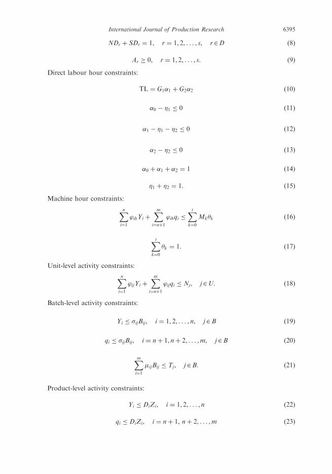
Direct labour hour constraints:

TL ¼ G1�1 þ G2�2 ð10Þ

�0 � �1 � 0 ð11Þ

�1 � �1 � �2 � 0 ð12Þ

�2 � �2 � 0 ð13Þ

�0 þ �1 þ �2 ¼ 1 ð14Þ

�1 þ �2 ¼ 1: ð15Þ

Machine hour constraints:

Xni¼1

’ihYi þXmi¼nþ1

’ihqi �Xtk¼0

Mkk ð16Þ

Xtk¼0

k ¼ 1: ð17Þ

Unit-level activity constraints:

Xni¼1

’ijYi þXmi¼nþ1

’ijqi � Nj, j2U: ð18Þ

Batch-level activity constraints:

Yi � �ijBij, i ¼ 1, 2, . . . , n, j2B ð19Þ

qi � �ijBij, i ¼ nþ 1, nþ 2, . . . ,m, j2B ð20Þ

Xmi¼1

�ijBij � Tj, j2B: ð21Þ

Product-level activity constraints:

Yi � DiZi, i ¼ 1, 2, . . . , n ð22Þ

qi � DiZi, i ¼ nþ 1, nþ 2, . . . ,m ð23Þ


Xmi¼1

�ijZi � Qj, j2P ð24Þ

Yi � 0, i ¼ 1, 2, . . . , n ð25Þ

qi � 0, i ¼ nþ 1, nþ 2, . . . ,m: ð26Þ

Where:

(NDr , SDr) is an SOS1 set of 0–1 variables, r¼ 1, 2 , . . . , s, r2D;(�0, �1, �2) is an SOS2 set of non-negative variables;(�1, �2) is an SOS1 set of 0–1 variables;(0, 1, . . . , t) is an SOS1 set of 0–1 variables;Zi is 0–1 variable, i¼ 1, 2, . . . ,m; andBij is non-negative integer variable, i¼ 1, 2, . . . ,m, j2B.

The following is the detailed description of the above model:

. Total revenue

The terms in the first set of parentheses in Equation (1) represent total revenue of

old and new products. The first term is the revenue of n original products and the

second term is that of the new product.

. Total direct material cost

The terms in the second set of parentheses in Equation (1), i.e.,Ps

r¼1 lrArþPr2D lDrADr, represent total direct material cost with (r2D) and without (r =2 D)

a purchase discount, respectively. Equations (2)–(9) are the constraints associated

with the various kinds of materials. For a material with a purchase discount

condition (r2D), Equation (4) describes that the quantity of this material that

either did qualify or did not qualify of a purchase discount should satisfy its

necessary amount for producing each product. Equations (5) and (6) describe the

conditions that a purchase discount either did qualify or not. Equation (7) sets a

maximum quantity of a material with a purchase discount that can be ordered.

At last, Equation (8) ensures that one, and only one of the conditions described

by Equations (5) and (6) is in effect for each material.

. Total direct labour cost

The terms in the third set of parentheses in Equation (1), i.e., C1�1 þ C2�2,represent total direct labour cost of both old and new products. Equations (10)–

(15) are the constraints associated with direct labour. TL, in Equation (10),

is total direct labour hours we need, and its function depends on the case under

study. In this paper, we assume that the direct labour resource can be expanded

by using overtime work or additional night shift with a higher wage rate.

Thus, the total direct labour cost function will be a piecewise linear function

composed of two segments with different wage rates as shown in Figure 1.

In Equations (11)–(15), (�1, �2) is an SOS1 set of 0–1 variables within which

exactly one variable must be non-zero; (�0,�1,�2) is an SOS2 set of non-negative

variables within which at most two adjacent variables, in the order given to the


set, can be non-zero (Williams 1985). If �1¼ 1, then �2 ¼ 0, �2 ¼ 0, �0, �1� 1, and�0 þ �1 ¼ 1. Thus, total direct labour hours needed and total direct labour costare G1�1 and C1�1, respectively. This means that: (1) the point (G1�1, C1�1) is onthe first segment of the piecewise linear direct labour cost function; and (2) (G1�1,C1�1) is the linear combination of (0, 0) and (G1, C1). This also means that we willnot need the overtime work. On the other hand, if �2 ¼ 1, then �1 ¼ 0, �0 ¼ 0, �1,�2� 1, and �1 þ �2 ¼ 1. Thus, total direct labour hours needed and total directlabour cost are G1�1 þ G2�2 and C1�1 þ C2�2, respectively. This means that: (1)the point (G1�1 þ G2�2, C1�1 þ C2�2) is on the second segment of the piecewiselinear direct labour cost function; and (2) (G1�1 þ G2�2, C1�1 þ C2�2) is the linearcombination of (G1, C1) and (G2, C2). This also means that we will need theovertime work.

. Total direct machine cost

The terms in the fourth set of parentheses in Equation (1), i.e.,Pn

i¼1 ah’ihYiþPmi¼nþ1 ah’ihqi, represent total direct machine cost. As stated in Section 3.1,

we assume that the facility-level activity cost function is a stepwise function,discussed later, which varies with the machine hours.

. Total unit-level overhead activity cost

The term (Pn

i¼1

Pj2U aj’ijYi þ

Pmi¼nþ1

Pj2U aj’ijqi) in Equation (1) is total unit-

level overhead activity cost of various unit-level activities ( j2U ) needed byboth old and new products. Equation (18) is the capacity constraints for variousunit-level activities.

. Total batch-level overhead activity cost

The termPm

i¼1

Pj2B aj�ijBij in Equation (1) is total batch-level overhead activity

cost of various batch-level activities ( j2B) needed by both old and new products.Equations (19)–(21) are the constraints associated with various batch-levelactivities, where Equation (21) is the capacity constraints for various batch-levelactivities. For example, we may use ‘setup hours’ as the activity driver of thebatch-level activity ‘setup’ because each product needs different setup hours.In this case, Tj are the available setup hours, �ij are the needed setup hours forproduct i, Bij is the number of setups needed for product i, and �ij is the average

Cost

Labour Hour0

C1

C2

G1 G2

Figure 1. Direct labour cost in enhanced ABC product-mix decision model.


number of units in each setup batch. In fact, there may be a different numberof units in each setup batch for a specific product. However, we can use theaverage number of units for the purpose of planning. On the other hand, we mayuse ‘number of batches’ as the activity driver of the batch-level activity ‘setup’because the setup hours needed is the same for each product. In this situation,�ij can be set to 1 and Tj is the available number of setups.

. Total product-level overhead activity cost

The termPm

i¼1

Pj2P aj�ijZi in Equation (1) is total product-level overhead

activity cost of various product-level activities ( j2P) needed by both old and newproducts. Equations (22)–(24) are the constraints associated with various product-level activities. Equations (22) and (23) are the market demand constraints forold and new products, respectively and Equation (24) is the capacity constraintsfor various product-level activities. For example, we may use ‘number ofdrawings’ as the activity driver of the product-level activity ‘product design’.In this case, Qj is the available number of drawings for the firm’s capacity, and �ijis the number of drawings needed for product i. Since Zi is a 0–1 variable,the market demand constraint for product i (in Equation (22) or (23)) will existif Zi ¼ 1.

. Total facility-level overhead activity cost

The termPt

k¼0 Fkk in Equation (1) is total facility-level overhead activity costand Equations (16)–(17) are the associated constraints. For the purpose ofplanning, we assume that the cost function of facility-level activity is a stepwisefunction that varies with the machine-hours range. (0, 1, . . . , t) is an SOS1 set of0–1 variables within which exactly one variable must be non-zero (Williams 1985).If 0 ¼ 1, the current machine hour capacity M0 will not be expanded and thecurrent total facility-level activity cost is still F0. If v ¼ 1 (v 6¼ 0), we know thatthe capacity needs to be expanded to the vth level, i.e., Mv machine hours, andtotal facility-level activity cost will be increased to Fv.

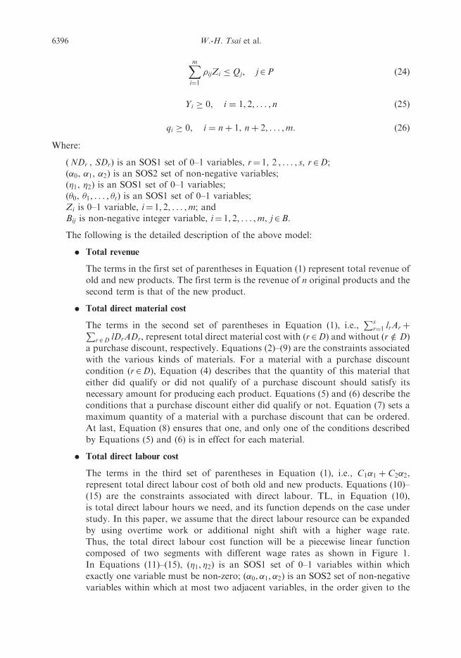
3.4 The product-mix decision model under TOC

In Kee (1995), and Kee and Schmidt (2000), a product-mix decision model under TOCselects a product mix based on maximising throughput, which is defined as a product’sprice less its direct material cost, while direct labour and overhead are treated as a fixedoperating expense. However, since the cost of capacity expansion is not a committedresource initially, the cost of capacity expansion should be treated as a variable. Therefore,for TOC, the product mix is selected by maximising the objective function shown inEquation (27) subject to the constraints in Equations (2)–(26) except Equations (10)–(15)which are replaced with Equations (28) and (29).

For the terms in the third set of parentheses in Equation (27), the cost of normal directlabour hours, C1, becomes fixed, but the direct labour resource can be expanded from G1

to G2 as shown in Figure 2. is a non-negative variable, where ðG2 � G1Þ and ðC2 � C1Þare the total expanded direct labour hours needed and the total expanded direct labourcost, respectively.

The terms from the fifth set to the last set of parentheses in Equation (27) represent thetotal overhead activity cost of the four levels respectively. The cost function of total direct


machine cost, i.e.,Pt

k¼0 ahMkk, and facility-level activity, i.e.,Pt

k¼0 Fkk, are assumed tobe stepwise functions that vary with the machine-hours range.

� ¼Xni¼1

piYi þXmi¼nþ1

piqi

!�

Xsr¼1

lrAr þXr2D

lDrADr

!

� C1 þ C2 � C1ð Þð Þ

�Xtk¼0

ahMkk �Xj2U

ajNj �Xj2B

ajTj �Xj2P

ajQj �Xtk¼0

Fkk ð27Þ

TL ¼ G1 þ G2 � G1ð Þ ð28Þ

� 0: ð29Þ

3.5 The enhanced general product-mix decision model

As indicated by Kee and Schmidt (2000), Equations (1) and (27) imply that managementhas either complete control or has no control over labour and overhead resources that aresomewhat extreme. Therefore, we propose an enhanced general model which incorporatesmanagement’s degree of control over resources together with capacity expansions andpurchase discount into the product-mix decision model as follows:

� ¼Xni¼1

piYi þXmi¼nþ1

piqi

!�

Xsr¼1

lrAr þXr2D

lDrADr

!

� ðNC1 þDC1�1 þ ðC2 �NC1Þ�2Þ

�Xtk¼0

ahðNMk þDM �k Þk �

Xj2U

ðaj ðNNj þDN �j ÞÞ

�Xj2B

ðaj ðNTj þDT �j ÞÞ

�Xj2P

ðaj ðNQj þDQ �j ÞÞ �Xtk¼0

Fkk: ð30Þ

Cost

Labour Hour0

C1

C2

G1 G2

Figure 2. Direct labour cost in enhanced TOC product-mix decision model.


Subject to:Direct material quantity constraints:

Xni¼1

birYi þXmi¼nþ1

birqi � Ar, r ¼ 1, 2, . . . , s, r =2 D ð31Þ

Ar �Wr, r ¼ 1, 2, . . . , s, r =2 D ð32Þ

Xni¼1

birYi þXmi¼nþ1

birqi � Ar þ ADr, r ¼ 1, 2, . . . , s, r2D ð33Þ

ADr � TDrSDr, r ¼ 1, 2, . . . , s, r2D ð34Þ

Ar 5TDrNDr, r ¼ 1, 2, . . . , s, r2D ð35Þ

ADr �WrSDr, r ¼ 1, 2, . . . , s, r2D ð36Þ

NDr þ SDr ¼ 1, r ¼ 1, 2, . . . , s, r2D ð37Þ

Ar � 0, r ¼ 1, 2, . . . , s: ð38Þ

Direct labour hour constraints:

TL ¼ NG1 þDG1�1 þ G2 �NG1ð Þ�2ð Þ ð39Þ

�0 � �1 � 0 ð40Þ

�1 � �1 � �2 � 0 ð41Þ

�2 � �2 � 0 ð42Þ

�0 þ �1 þ �2 ¼ 1 ð43Þ

�1 þ �2 ¼ 1: ð44Þ

Machine hour constraints:

Xni¼1

’ihYi þXmi¼nþ1

’ihqi �Xtk¼0

NM �k þDM �

k

� �k ð45Þ

Xtk¼0

NM �k k �

Xtk¼0

NMkk ð46Þ

Xtk¼0

DM �k k �

Xtk¼0

DMkk ð47Þ

Xtk¼0

NMk þDMkð Þk �Xtk¼0

Mkk ð48Þ


Xtk¼0

k ¼ 1: ð49Þ

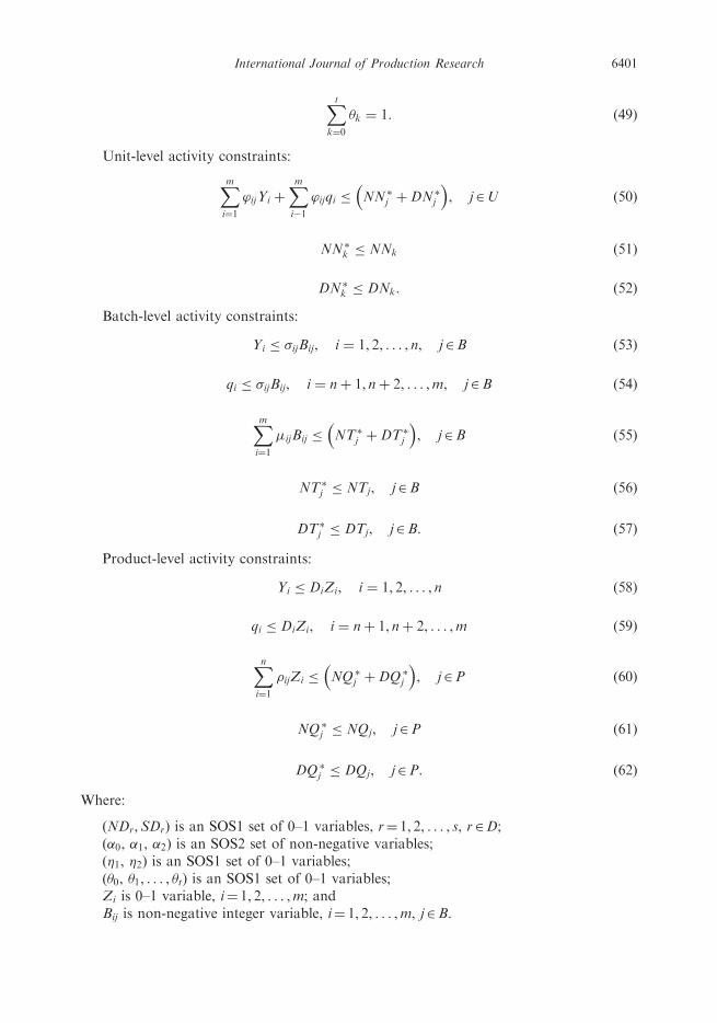
Unit-level activity constraints:

Xmi¼1

’ijYi þXmi�1

’ijqi � NN �j þDN �j

� �, j2U ð50Þ

NN �k � NNk ð51Þ

DN �k � DNk: ð52Þ

Batch-level activity constraints:

Yi � �ijBij, i ¼ 1, 2, . . . , n, j2B ð53Þ

qi � �ijBij, i ¼ nþ 1, nþ 2, . . . ,m, j2B ð54Þ

Xmi¼1

�ijBij � NT �j þDT �j

� �, j2B ð55Þ

NT �j � NTj, j2B ð56Þ

DT �j � DTj, j2B: ð57Þ

Product-level activity constraints:

Yi � DiZi, i ¼ 1, 2, . . . , n ð58Þ

qi � DiZi, i ¼ nþ 1, nþ 2, . . . ,m ð59Þ

Xni¼1

�ijZi � NQ �j þDQ �j

� �, j2P ð60Þ

NQ �j � NQj, j2P ð61Þ

DQ �j � DQj, j2P: ð62Þ

Where:

(NDr,SDr) is an SOS1 set of 0–1 variables, r¼ 1, 2, . . . , s, r2D;(�0, �1, �2) is an SOS2 set of non-negative variables;(�1, �2) is an SOS1 set of 0–1 variables;(0, 1, . . . , t) is an SOS1 set of 0–1 variables;Zi is 0–1 variable, i¼ 1, 2, . . . ,m; andBij is non-negative integer variable, i¼ 1, 2, . . . ,m, j2B.


We assume that direct material is a variable cost and facility-level activity is a fixed costas prior studies did. For other resources, management may have different discretionarypower. Therefore, we use DC1, DMk, DNj, DTj, and DQj to denote the amount ofresources which subject to management control, and use NC1, NMk, NNj, NTj, and NQj

to denote the amount of resources which do not subject to management control, whileDC �1 , NC �1 , DM �

k , NM �k , DN �j , NN �j , DT �j , NT �j , DQ �j , and NQ �j represent the amount

of those resources that are consumed in production.The objective function in Equation (30) incorporates the resources that management

has no control over as a fixed cost and the resources over which management has controlthat is used in production as a product cost. The constraints in Equations (45)–(62) statethat different kinds of resources used in production must under the sum of the amountof those resources which are non-discretionary and the amount of those resources whichare discretionary and are used in production. The amounts of resources which have nocontrol over and control over are also restricted by the constraints in Equations (45)–(62).

The normal direct labour hours are separated into two parts: non-discretionarylabour hours and discretionary labour hours as shown in Figure 3. The terms in the thirdset of parentheses in Equation (30), i.e., ðNC1 þDC1�1 þ ðC2 �NC1Þ�2Þ, representtotal direct labour cost of both old and new products, where NC1 represents the costof non-discretionary labour hours, and DC1�1 þ ðC2 �NC1Þ�2 represents the sum of thecost of discretionary labour hours and the cost of overtime work. The functions ofEquations (40)–(44) are similar to the Equations (11)–(15) in the enhanced ABC model.

4. A numerical illustration

4.1 Data and description of a numerical example

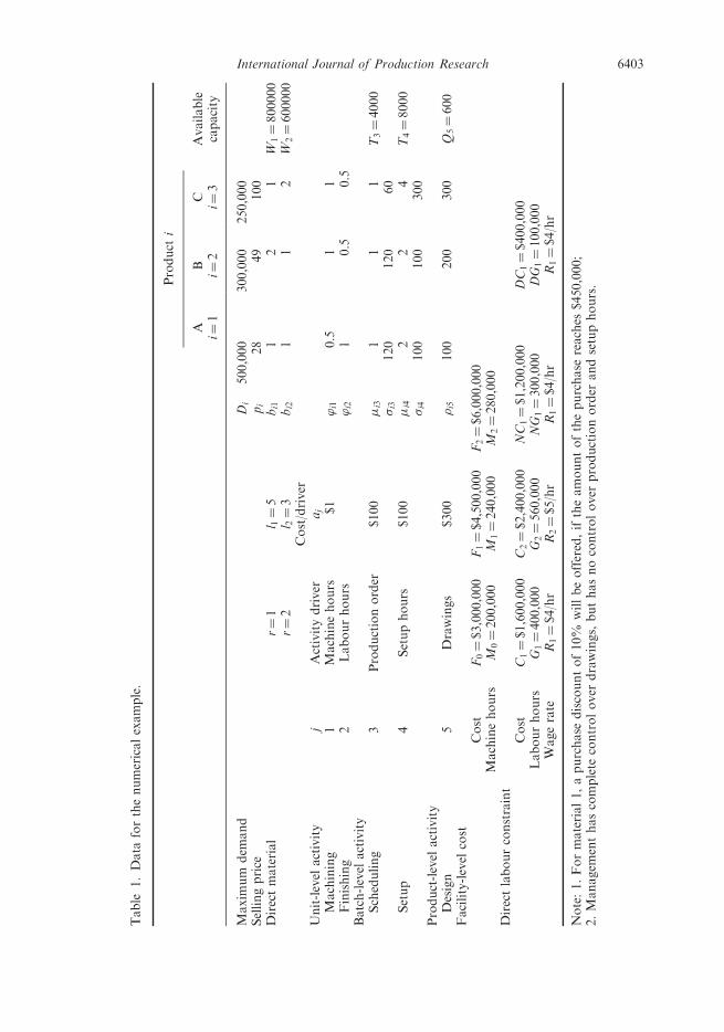
This paper provides a numerical example to apply the product-mix decision models.The data and background of this example are described as follows.

Let us assume that a company produces two products, A (i¼ 1) and B (i¼ 2), and plansto launch a new product C (i¼ 3). Each product requires the processing of five primaryactivities, of which, two activities are performed at the unit-level, two at the batch-leveland one at the product-level. Three products consume two types of direct material. Thevendor of material 1 allows a purchase discount of 10% if the amount of the purchasereaches $450,000. Table 1 shows the data in this example. In Table 1, M0 stands for thecurrent machine capacity, 200,000 machine hours, and F0 represents the facility-level

Cost

Labour Hour0

C1

C2

DG1 G2NG1

Figure 3. Direct labour cost in enhanced general product-mix decision model.


Table

1.Data

forthenumericalexample.

Product

i

Available

capacity

AB

Ci¼

1i¼

2i¼

3

Maxim

um

dem

and

Di

500,000

300,000

250,000

Sellingprice

pi

28

49

100

Directmaterial

r¼1

l 1¼5

bi1

12

1W

1¼800000

r¼2

l 2¼3

bi2

11

2W

2¼600000

Cost/driver

Unit-level

activity

jActivitydriver

aj

Machining

1Machinehours

$1

’i1

0.5

11

Finishing

2Labourhours

’i2

10.5

0.5

Batch-level

activity

Scheduling

3Productionorder

$100

�i3

11

1T3¼4000

�i3

120

120

60

Setup

4Setuphours

$100

�i4

22

4T4¼8000

�i4

100

100

300

Product-level

activity

Design

5Drawings

$300

�i5

100

200

300

Q5¼600

Facility-level

cost

Cost

F0¼$3,000,000

F1¼$4,500,000

F2¼$6,000,000

Machinehours

M0¼200,000

M1¼240,000

M2¼280,000

Directlabourconstraint

Cost

C1¼$1,600,000

C2¼$2,400,000

NC

1¼$1,200,000

DC

1¼$400,000

Labourhours

G1¼400,000

G2¼560,000

NG

1¼300,000

DG

1¼100,000

Wagerate

R1¼$4/hr

R2¼$5/hr

R1¼$4/hr

R1¼$4/hr

Note:1.Formaterial1,apurchase

discountof10%

willbeoffered,iftheamountofthepurchase

reaches

$450,000;

2.Managem

enthascomplete

controlover

drawings,buthasnocontrolover

productionorder

andsetuphours.


activity cost, $3,000,000 at this capacity level. To increase the machine capacity from M0

toM1 orM2, the company needs to lease machines from vendors and, as a result, increasesthe facility-level cost to $4,500,000 (F1) or $6,000,000 (F2). Normal direct labour hours,G1, is 400,000 hours, and the wage rate is $4 per hour. In the 400,000 direct labour hours,300,000 of them come from formal employees that are non-discretionary, while the other100,000 come from temporary workers that are discretionary. The direct labour hourscan be expanded to G2¼ 560,000 hours by using overtime work and the wage rate will be$5 per hour. In this case, total direct labour hours (TL), can be depicted by the followingequation:

Xni¼1

’i2Yi þXmi¼nþ1

’i2qi ¼ G1�1 þ G2�2: ð63Þ

In this example, management has complete control over drawings, but has no controlover production order and setup hours.

4.2 Three-part analysis

4.2.1 Part 1: determining the optimal product-mix and capacity expansion before addingnew products

The objective of this part is to find the optimal product-mix that maximises the company’sprofit prior to adding a new product into the product-mix. Based on the informationprovided in Table 1, this part applies the three proposed models, which are 0–1 mixed-integer programming models and can be solved by the software ‘LINGO’, and ignores thenew product C’s information. Table 2 shows the objective function, related constraintsbefore adding a new product into the product-mix of the three models.

A comparison of the optimal solutions of the three models is shown in Table 3.In Table 3, panel 1, the product mix, the resources used in production, the unusedresources, and the capacity expansions are compared, while an income statement for theproduct mix selected with the three models is shown in Table 3, panel 2. According toTable 3, panel 2, the product mix selected with ABC has the highest income based onthe resources used in production. However, when the cost of unused non-discretionaryresources was deducted from revenue, the product mix selected with the enhanced generalmodel leads to the highest income.

4.2.2 Part 2: determining the optimal product-mix after adding new products

Generally, the initial production volume of a new product is lower because the companyis unaware of the condition of market acceptance. Over a period of time, when the newproduct receives positive evaluation from customers, the company then takes expandedaction. Additionally, the company will gradually transfer production resources from oldproducts to new products. However, the company’s production policy in old products stillmaintains at specific volumes to keep the old customers.

The company should evaluate carefully for new product’s price orientation in themarket. Based on the information provided in Table 1, this part applies our enhancedgeneral model, Equations (30) to (62), and other constraints (i.e., new product’s price isequal to 70 (p3¼ 70) and old products’ production volumes are greater than or equal to500 units respectively (Y1� 500, Y2� 500)) to explore the optimal product-mix.


Table 2. Decision analysis prior to adding the new product into the product-mix (only two originalproducts).

Enhanced ABC product-mix decision model

Maximise�¼ 28Y1þ 49Y2� 5M1� 4.5MD1� 3M2� 1,600,000�1� 2,400,000�2� 0.5Y1� Y2� 100B13� 100B23� 200B14� 200B24� 30,000Z1� 60,000Z2

� 3,000,0000� 4,500,0001� 6,000,0002

Subject to—direct material Subject to—machine hourY1þ 2Y2�M1�MD1� 0 0.5Y1þY2� 200,0000� 240,0001� 280,0002 � 0Y1þY2�M2� 0 0þ 1þ 2¼ 1

M1� 0 Subject to—batch-level activity (scheduling)M15 4500,000ND1 Y1� 120B13� 0MD1� 450,0000SD1 Y2� 120B23� 0MD1� 800,000SD1 B13þB23� 4000

ND1þSD1¼ 1 Subject to—batch-level activity (setup)M2� 0 Y1� 100B14� 0M2� 600,000 Y2� 100B24� 0

2B14þ 2B24� 8000

Subject to—direct labour Subject to—product-level activity (design)Y1þ 0.5Y2� 400,000�1� 560,000�2 � 0 Y1� 500,000Z1� 0�0� �1 � 0 Y2� 300,000Z2� 0�1� �1� �2� 0 100Z1þ 200Z2 � 600�2� �2 � 0�0þ �1þ�2¼ 1�1þ �2¼ 1

Enhanced TOC product-mix decision model

Maximise�¼ 28Y1þ 49Y2� 5M1� 4.5MD1� 3M2� 1,600,000� 800,000� 200,0000� 240,0001� 280,0002� 400,000� 800,000� 180,000� 3,000,0000� 4,500,0001� 6,000,0002

Subject to—direct material Subject to—machine hourY1þ 2Y2�M1�MD1� 0 0.5Y1þY2� 200,0000� 240,0001� 280,0002 � 0Y1þY2�M2 � 0 0þ 1þ 2¼ 1

M1� 0 Subject to—batch-level activity (scheduling)M1 5 4500,000ND1 Y1� 120B13� 0MD1 � 450,0000SD1 Y2� 120B23� 0MD1 � 800,000SD1 B13þB23� 4000


2B14þ 2B24� 8000

Subject to—direct labour Subject to—product-level activity (design)Y1þ 0.5Y2� 400,000� 160,000� 0 Y1� 500,000Z1� 0 � 0 Y2� 300,000Z2� 0

100Z1þ 200Z2 � 600

(continued )


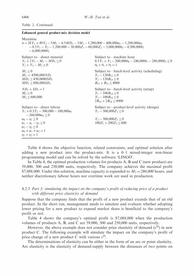
Table 4 shows the objective function, related constraints, and optimal solution afteradding a new product into the product-mix. It is a 0–1 mixed-integer non-linearprogramming model and can be solved by the software ‘LINGO’.

In Table 4, the optimal production volumes for products A, B and C (new product) are59,000, 500 and 250,000 units, respectively. The company achieves the maximal profit$7,088,000. Under this solution, machine capacity is expanded to M2¼ 280,000 hours, andneither discretionary labour hours nor overtime work are used in production.

4.2.3 Part 3: simulating the impact on the company’s profit of reducing price of a productwith different price elasticity of demand

Suppose that the company finds that the profit of a new product exceeds that of an oldproduct. In the short run, management needs to simulate and evaluate whether adoptinglower pricing for a new product to expand market share is beneficial to the company’sprofit or not.

Table 4 shows the company’s optimal profit is $7,088,000 when the productionvolumes of products A, B, and C are 59,000, 500 and 250,000 units, respectively.

However, the above example does not consider price elasticity of demand ("D) in newproduct C. The following example will simulate the impact on the company’s profit ofprice change of a new product C with various "D.

The determinations of elasticity can be either in the form of an arc or point elasticity.Arc elasticity is the elasticity of demand/supply between the distances of two points on

Table 2. Continued.

Enhanced general product-mix decision model

Maximise�¼ 28Y1þ 49Y2� 5M1� 4.5MD1� 3M2� 1,200,000� 400,000�1� 1,200,000�2� 0.5Y1�Y2� 1,200,000� 30,000Z1� 60,000Z2� 3,000,0000� 4,500,0001� 6,000,0002

Subject to—direct material Subject to—machine hourY1þ 2Y2�M1�MD1� 0 0.5Y1þY2� 200,0000� 240,0001� 280,0002� 0Y1þY2�M2 � 0 0þ 1þ 2¼ 1

M1� 0 Subject to—batch-level activity (scheduling)M1 5 4500,000ND1 Y1� 120B13� 0MD1 � 450,0000SD1 Y2� 120B23� 0MD1 � 800,000SD1 B13þB23� 4000


2B14þ 2B24� 8000

Subject to—direct labour Subject to—product-level activity (design)Y1þ 0.5Y2� 300,000� 100,000�1� 260,000�2 � 0

Y1� 500,000Z1 � 0

�0� �1 � 0 Y2� 300,000Z2 � 0�1� �1� �2� 0 100Z1þ 200Z2 � 600�2� �2 � 0�0þ �1þ�2¼ 1�1þ �2¼ 1


a demand/supply curve. In this paper, the concept of arc elasticity is used to measure price

elasticity of demand. The price elasticity of demand "D is defined as the following

equation:

"D ¼ �Dq�12 ðq0 þ qÞ

Dp�12 ð p0 þ pÞ

!

¼ �Dq= �q

Dp= �p

� �:

ð64Þ

Table 3. A comparison between the optimal solutions of the three models.

TOC ABC General-model

Panel 1: product-mixProduct mixA 400,000 0 240,000B 0 200,000 120,000

Resource used in productionDirect material 1 400,000 400,000 480,000Direct material 2 400,000 200,000 360,000Non-discretionary direct labour hours 300,000 100,000 300,000Discretionary direct labour hours 100,000 0 0Direct machine hours 200,000 200,000 240,000Production order 3334 1667 3000Setup hours 8000 4000 7200Engineering drawings 100 200 300

Unused resourcesNon-discretionary direct labour hours 0 200,000 0Discretionary direct labour hours 0 100,000 100,000Direct machine hours 0 0 0Production order 666 2333 1,000Setup hours 0 4000 800Engineering drawings 500 400 300

Capacity expansionMachine capacity 0 0 40,000Overtime work 0 0 0

Panel 2: product-mix income

Revenue 11,200,000 9,800,000 12,600,000Cost of resource used in productionDirect material 1 2,000,000 2,000,000 2,160,000Direct material 2 1,200,000 600,000 1,080,000Non-discretionary direct labour hours 1,200,000 400,000 1,200,000Discretionary direct labour hours 400,000 0 0Direct machine hours 200,000 200,000 240,000Production order 333,400 166,700 300,000Setup hours 800,000 400,000 720,000Engineering drawings 30,000 60,000 90,000Facility-level cost 3,000,000 3,000,000 4,500,000

Income based on resources used 2,036,600 2,973,300 2,310,000Cost of unused non-discretionary resource 66,600 1,433,300 180,000Net income 1,970,000 1,540,000 2,130,000


In calculating the price elasticity, we use the average of the original and new price, i.e.,�p ; similarly for the quantity demanded, we use �q. An elasticity computed by this method

is called an arc elasticity of demand (Pindyck and Rubinfeld 1998). Where p represents

the selling price, and p0 represents that of after change; Dp (i.e., p0 � p) is a change in price;

q represents the quantity demanded of new product before change, and q0 represents that

of after change; Dq (i.e., q0 � q) is induced change in the quantity demanded.This paper assumes that "D value of new product C is varied from 0.25 to 1000.

Additionally, the company adopts a lower pricing strategy to stimulate demand, and the

company’s plant is able to supply the product as needed. Thus, the following equation

is added into the product-mix decision model:

"D ¼ �Dq3

�12 q03 þ q3� �

Dp3�12 p03 þ p3� �

!¼ k, k ¼ 0:25, 1, 5:286, 20, 40, 1000: ð65Þ

Table 4. Decision analysis of the enhanced general product-mix decision model after adding a newproduct.

Maximise�¼ 28Y1þ 49Y2þ p3q3� 5M1� 4.5MD1� 3M2� 1,200,000� 400,000�1� 1,200,000�2� 0.5Y1�Y2� q3� 400,000� 800,000� 30,000Z1� 60,000Z2� 90,000Z3� 3,000,0000� 4,500,0001� 6,000,0002

Subject to—direct material Subject to—batch-level activity (scheduling)Y1þ 2Y2þ q3�M1�MD1� 0 Y1� 120B13� 0Y1þY2þ 2q3�M2 � 0 Y2� 120B23� 0M1� 0 Y3� 90B33� 0M1 5 450,000ND1 B13þB23þB33� 4000MD1 � 450,0000SD1 Subject to—batch-level activity (setup)MD1 � 800,000SD1 Y1� 100B14� 0ND1þSD1¼ 1 Y2� 100B24� 0M2� 0 Y3� 300B34� 0M2� 600,000 2B14þ 2B24þ 4B34� 8000

Subject to—direct labour Subject to—product-level activity (design)Y1þ 0.5Y2þ 0.5q3� 300,000� 100,000�1� 260,000�2 � 0

Y1� 500,000Z1 � 0

�0� �1 � 0 Y2� 300,000Z2 � 0�1� �1� �2� 0 Y3� 250,000Z3 � 0�2� �2 � 0 100Z1þ 200Z2þ 300Z3 � 600�0þ �1þ�2¼ 1�1þ �2¼ 1

Other constraint (1)—p3¼ 100Other constraint (2)—Y1 � 500Y2� 500

Subject to—machine hour0.5Y1þY2þ q3� 200,0000� 240,0001

� 280,0002 � 00þ 1þ 2¼ 1

Optimal solution is as follows: �¼ 7,088,000, Y1¼ 59,000, Y2¼ 500, p3¼ 70, q3¼ 250,000,M1¼ 310,000, MD1¼ 0, M2¼ 559,500, ND1¼ 1, SD1¼ 0, �0¼ 1, �1¼ 0, �2¼ 0, B13¼ 492,


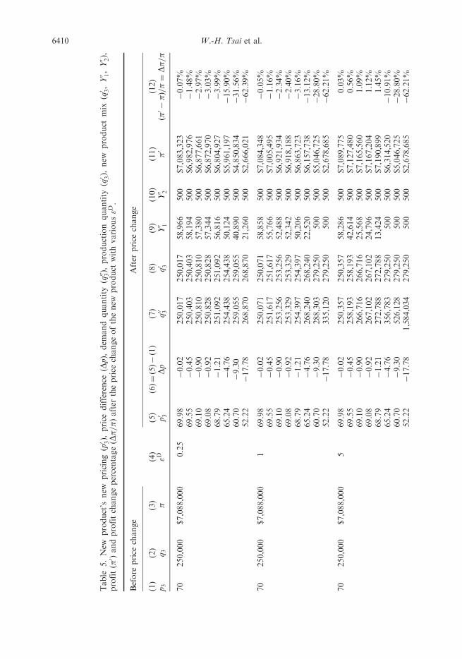
Under a different k value, we could formulate the constraint of "D 1. Assume "D ofproduct C has six different situations (see column (4) of Table 5), and reducing priceof product C has eight possibilities (see columns (5) and (6) of Table 5). According to thisinformation, we could obtain demand quantity information of product C while reducingthe price at different "D from column (7) of Table 5.

For most goods, the lower the price the more customers will demand or purchase,because the demand curve is downward sloping. Furthermore, the greater "D value in theproduct the more customers will demand or purchase by a lower price. On columns (4) to(7) of Table 5, if new pricing (p03) of product C is 99.98 (reducing price $0.02), then demandquantity for product C will be 250,017 to 333,347 units in "D varied from 0.25 to 1000.On column (8) of Table 5, we can see that even the demand quantity of product C increaseswith the price1 of product C decrease, the maximal production volumes of product Cis 279,250 under the capacity and production constraints listed in Table 4. In columns (8)to (10) of Table 5, this symbol (—) represents the demand quantity of product C exceedsthe boundary of general integer of LINGO.

In general, the company’s production policy will be based on the maximising profit ruleinstead of only considering customers’ demand. However, management needs to simulateand evaluate whether adopting lower pricing for a new product is beneficial to thecompany’s profit or not.

It is important for management to not only consider the impact of "D and reducing theprice for new product C, but to also evaluate the impact on the company’s aggregate profitof price change. The details about a new product’s new price (p03), price difference (Dp),demand quantity (q003), production quantity (q03), new product mix (q03, Y

01, Y

02), profit (�

0)and profit change percentage are shown in Table 5. Table 5 shows product C’s initialselling price is 70 when the company produces 250,000 units of product C. Suppose thatthe company plans to increase product C’s production volumes from 250,000 to at least262,500 units (q03� 262,500), i.e., increasing 5% market share. In Table 5, left and rightsides for "D column represent the information before and after a price change in productC, respectively. According to the earlier eighth assumption, this study implies that thecompany produces the old and new products based on aggregate market demand andrelated cost information of products. Column (8) of Table 5 represents product C’sproduction quantity maximising company’s profit after a price change. For example, when"D of product C is equal to 20 and the new pricing of product C is 69.10 (reducing the priceby $0.9), the customer will demand 324,318 units of product C. In this situation, theproduction quantity of products A, B, and C are 500, 500, and 279,250 units, respectively,and the company could increase profits compared to before the price change (increasingprofit 4.29%).

On the contrary, observing "D¼ 1 situation in Table 5, if the company produces268,240 units of product C (selling price $65.24), 22,520 units of product A (Y01¼ 22,520)and 500 units of product B (Y02¼ 500), then this company’s profit is $6,157,738, lower thanthe product-mix’s profit (�¼ $7,088,000) before the price change. The same situationhappens on "D¼ 0.25 of Table 5. Suppose that the company plans to increase product C’sproduction volume from 250,000 to at least 262,500 units (q03� 262,500), i.e., increasing5% market share. In Table 5 for "D¼ 0.25 for p03¼ 52.22 the values for q03, Y01, Y02,(the optimal product-mix) and �0 are 268,870, 21,260, 500 and $2,666,021, respectively,lower than the product-mix’s profit (�¼ $7,088,000) before the price change. Thissituation indicates product C having "D¼ 0.25 in this case is not appropriate for reducingprice from profit view. If the current strategy of the company is to upgrade market share


Table

5.New

product’s

new

pricing(p0 3),

price

difference

(Dp),

dem

and

quantity

(q00 3),

production

quantity

(q0 3),

new

product

mix

(q0 3,Y0 1,Y0 2),

profit(�0 )andprofitchangepercentage(D�=�

)after

theprice

changeofthenew

product

withvarious"D

.

Before

price

change

After

price

change

(1)

(2)

(3)

(4)

"D(5)

(6)¼(5)�(1)

(7)

(8)

(9)

(10)

(11)

(12)

p3

q3

�p0 3

Dp

q00 3

q0 3

Y0 1

Y0 2

�0

ð�0��Þ=�¼

D�=�

70

250,000

$7,088,000

0.25

69.98

�0.02

250,017

250,017

58,966

500

$7,083,323

�0.07%

69.55

�0.45

250,403

250,403

58,194

500

$6,982,976

�1.48%

69.10

�0.90

250,810

250,810

57,380

500

$6,877,661

�2.97%

69.08

�0.92

250,828

250,828

57,344

500

$6,872,970

�3.03%

68.79

�1.21

251,092

251,092

56,816

500

$6,804,927

�3.99%

65.24

�4.76

254,438

254,438

50,124

500

$5,961,197

�15.90%

60.70

�9.30

259,055

259,055

40,890

500

$4,850,834

�31.56%

52.22

�17.78

268,870

268,870

21,260

500

$2,666,021

�62.39%

70

250,000

$7,088,000

169.98

�0.02

250,071

250,071

58,858

500

$7,084,348

�0.05%

69.55

�0.45

251,617

251,617

55,766

500

$7,005,495

�1.16%

69.10

�0.90

253,256

253,256

52,488

500

$6,921,934

�2.34%

69.08

�0.92

253,329

253,329

52,342

500

$6,918,188

�2.40%

68.79

�1.21

254,397

254,397

50,206

500

$6,863,723

�3.16%

65.24

�4.76

268,240

268,240

22,520

500

$6,157,738

�13.12%

60.70

�9.30

288,303

279,250

500

500

$5,046,725

�28.80%

52.22

�17.78

335,120

279,250

500

500

$2,678,685

�62.21%

70

250,000

$7,088,000

569.98

�0.02

250,357

250,357

58,286

500

$7,089,775

0.03%

69.55

�0.45

258,193

258,193

42,614

500

$7,127,480

0.56%

69.10

�0.90

266,716

266,716

25,568

500

$7,165,560

1.09%

69.08

�0.92

267,102

267,102

24,796

500

$7,167,204

1.12%

68.79

�1.21

272,788

272,788

13,424

500

$7,190,899

1.45%

65.24

�4.76

356,783

279,250

500

500

$6,314,520

�10.91%

60.70

�9.30

526,128

279,250

500

500

$5,046,725

�28.80%

52.22

�17.78

1,584,034

279,250

500

500

$2,678,685

�62.21%


70

250,000

$7,088,000

20

69.98

�0.02

251,432

251,432

56,136

500

$7,110,179

0.31%

69.55

�0.45

284,469

279,250

500

500

$7,518,088

6.07%

69.10

�0.90

324,318

279,250

500

500

$7,392,425

4.29%

69.08

�0.92

326,234

279,250

500

500

$7,386,840

4.22%

68.79

�1.21

355,593

279,250

500

500

$7,305,858

3.07%

65.24

�4.76

1,438,811

279,250

500

500

$6,314,520

�10.91%

60.70

�9.30

——

——

52.22

�17.78

——

——

70

250,000

$7,088,000

40

69.98

�0.02

252,874

252,873

53,254

500

$7,137,530

0.70%

69.55

�0.45

324,043

279,250

500

500

$7,518,088

6.07%

69.10

�0.90

424,587

279,250

500

500

$7,392,425

4.29%

69.08

�0.92

429,898

279,250

500

500

$7,386,840

4.22%

68.79

�1.21

517,728

279,250

500

500

$7,305,858

3.07%

65.24

�4.76

——

——

60.70

�9.30

——

——

52.22

�17.78

——

——

70

250,000

$7,088,000

1,000

69.98

�0.02

333,347

279,250

500

500

$7,638,165

7.76%

69.55

�0.45

——

——

69.10

�0.90

——

——

69.08

�0.92

——

——

68.79

�1.21

——

——

65.24

�4.76

——

——

60.70

�9.30

——

——

52.22

�17.78

——

——

Note:Thesymbol(—

)represents

thedem

andquantity

ofproduct

Cexceedstheboundary

ofgeneralinteger

ofLIN

GO.


at a goal volume (i.e., at least q03� 262,500), then the company will decrease more profitto trade-off market share comparing to before price change (decreasing profit 62.39%).Note that for a price of p03¼ 69.98 and p03¼ 52.22 in "D¼ 0.25, the profits of both product-mix are lower than the profit before the price change. In this case, the company ought notto adopt reducing price strategy for product C having "D¼ 0.25 to expand market share,because it will decrease the company’s total profit.

The above situation illustrates that the company cannot arbitrarily adopt lowerpricing strategy to expand market share because the company’s profit growth rate (D�=�)is negative when "D value of a new product is lower than a specific value. This numericalexample shows the importance of considering the price elasticity of demand. The moremanagement realises the elasticity of a company’s product, the more management adoptsan appropriate price strategy. Some economics professors often use Starbucks as anexample of a company whose product seems to have little price elasticity. Starbuck’smanagement agrees with those professors and thinks the demand of Starbuck’s product isinelastic, meaning that a price change will cause less of a change in quantity demanded.Maybe, that is one reason behind Starbuck’s success, because Starbuck’s managementfully realises their products’ characteristics. Generally, the price elasticity of demand isaffected by factors such as those listed below:

. Availability of substitutes: the more possible substitutes, the greater the elasticity.

. Degree of necessity or luxury: luxury products tend to have greater elasticity.Some products that initially have a low degree of necessity are habit forming andcan become ‘necessities’ to some consumers.

. Proportion of the purchaser’s budget consumed by the item: products that consumea large portion of the purchaser’s budget tend to have greater elasticity.

. Time period considered: elasticity tends to be greater over the long run becauseconsumers have more time to adjust their behaviour.

. Permanent or temporary price change: a one-day sale will elicit a different responsethan a permanent price decrease.

According to available information, the company can examine price elasticity ofrelated products, and develop an appropriate pricing strategy for a particular productto increase its market share and profit.

5. Concluding remarks

This paper developed an enhanced general model that incorporates all four factors:capacity constraint, management’s degree of control over resource, capacity expansions,and purchase discount to determine the optimal product-mix.

Establishing a general model related to ABC product-mix decisions is still limited in thecurrent ABC literature. This paper tried to develop a more realistic product-mix decisionmodel under ABC and discussed the related-analysis for adding a new product intothe present product-mix. This paper integrated factors proposed in related works andconsidered an important feature in practice: price elasticity of demand and the capacityexpansion. This paper also provided a comprehensive illustration on how a company usesthe mathematical programming approach to obtain the optimal product-mix and thecapacity expansion to achieve profit goals. Additionally, this paper used a numericalexample to simulate the impact on the company’s profit for reducing the price of a productwith different "D.


This paper was based on some specific assumptions. For example, this paper assumedthat potential competitors’ prices are not sensitive to temporary price changes of acompany’s product in the short term. In future studies, researchers can relax assumptionsto explore more complicated and realistic situations.

Acknowledgement

This study was supported by National Science Council of Taiwan under grant NSC90-2416-H-008-001.

Note

1. For example, when "D¼ 1, we then have the following equation by using Equation (65):

q03 � q3� �

p3 þ p03� �

¼ q3 þ q03� �

p3 � p03� �

! q03p3 þ q03p03 � q3p3 � q3p

03

� �¼ q3p3 � q3p

03 þ q03p3 � q03p

03

� �! 2q03p

03 ¼ 2q3p3

! q03p03 ¼ q3p3:

Assuming that p3¼ 70, q3¼ 250,000, then q03p03^ 17,500,000 (the constraint when "D¼ 1).

References

Antos, J., 1992. Activity-based management for service, not-for-profit, and governmental

organizations. Journal of Cost Management, 6 (2), 13–23.Banker, R. and Hughes, J., 1994. Product cost and pricing. Accounting Review, 69 (3), 479–494.Bakke, N. and Hellberg, R., 1991. Relevance lost? A critical discussion of different cost accounting

principles in connection with decision making for both short and long term production

scheduling. International Journal of Production Economics, 24 (1–2), 1–18.Bhatnagar, R., et al., 1999. Order release and product mix co-ordination in a complex PCB

manufacturing line with batch processors. International Journal of Flexible Manufacturing

Systems, 11 (4), 327–351.Brewer, P.C., Juras, P.E., and Brownlee II, E.R., 2003. Global Electronics, Inc.: ABC implemen-

tation and change management process. Issues in Accounting Education, 18 (1), 49–69.Campbell, R., Brewer, P., and Mills, T., 1997. Designing an information system using activity-based

costing and the theory of constraints. Journal of Cost Management, 11 (1), 16–25.Carlson, D.A. and Young, S.M., 1993. Activity-based total quality management at American

Express. Journal of Cost Management, 7 (1), 48–58.Carter, W.K. and Usry, M.F., 2002. Cost accounting. 13th ed. London: Dame/Thomson Learning.Chan, Y.-C., 1993. Improving hospital cost accounting with activity-based costing. Health Care

Management Review, 18 (1), 71–77.Charnes, A., Cooper, W.W., and Ijiri, Y., 1963. Break-even budgeting and programming to goals.

Journal of Accounting Research, 1 (1), 16–43.

Chomiakow, D., 2007. A generic pattern for modeling manufacturing companies. In: Proceedingsof the 2007 international conference of the System Dynamics Society and 50th anniversary

celebration. 29 July–2 August Boston, Massachusetts, 71.Chou, Y.C. and Hong, I.H., 2000. A methodology for product mix planning in semiconductor

foundry manufacturing. IEEE Transactions on Semiconductor Manufacturing, 13 (3), 278–285.Cooper, R. and Kaplan, R.S., 1988a. How cost accounting distorts product costs. Management

Accounting, 69 (10), 20–27.


Cooper, R. and Kaplan, R.S., 1988b. Measure costs right: make the right decisions. Harvard

Business Review, 66 (5), 96–103.

Cooper, R., 1989. The rise of activity-based costing – part four: what do activity-based cost system

look like? Journal of Cost Management, 3 (1), 38–49.

Cooper, R., 1990. Cost classification in unit-based and activity-based manufacturing cost systems.

Journal of Cost Management, 4 (3), 4–14.

Cooper, R. and Kaplan, R.S., 1991. Profit priorities from activity-based costing. Harvard Business

Review, 69 (3), 130–135.

Cooper, R. and Kaplan, R., 1992. Activity-based-systems: measuring the costs of resource usage.

Accounting Horizons, 6 (3), 1–13.

Cooper, R., et al., 1992. From ABC to ABM: does activity-based management automatically follow

from an activity-based costing project? Management Accounting, 74 (5), 54–57.

Dhavale, D.G., 1993. Activity-based costing in cellular manufacturing systems. Journal of Cost

Management, 7 (1), 13–27.

Fichman, R.G. and Kemerer, C.F., 2002. Activity based costing for component-based software

development. Information Technology and Management, 3 (1–2), 137–160.

Field, M.K. and Pagoulatos, E., 1997. The cyclical behavior of price elasticity of demand. Southern

Economic Journal, 64 (1), 118–129.

Foster, G. and Swenson, D., 1997. Measuring the success of activity-based cost management and its

determinants. Journal of Management Accounting Research, 9, 109–141.

Goldratt, E.M., 1990. Theory of constraints: what is this thing called theory of constraints and how

should it be implemented? Croton-on-Hudson, NY: North River Press.

Harr, D.J., 1990. How activity accounting works in government. Management Accounting, 72 (3),

36–40.

Holmen, J., 1995. ABC vs. TOC: it’s a matter of time activity-based costing and the theory of

constraints can work together. Management Accounting, 76 (7), 37–40.

Innes, J., Mitchell, F., and Sinclair, D., 2000. Activity-based costing in the UK’s largest companies:

a comparison of 1994 and 1999 survey results. Management Accounting Research, 11 (3),

349–362.Johnson, H., 1992. It’s time to stop overselling activity-based concepts. Management Accounting,

74 (3), 26–35.Kaplan, R., 2005. Activity-based costing and capacity. Technical note #9-105-059. Boston, MA:

Harvard Business School.Kee, R., 1995. Integrating activity-based costing with the theory of constraints to enhance

production-related decision-making. Accounting Horizons, 9 (12), 48–61.Kee, R. and Schmidt, C., 2000. A comparative analysis of utilizing activity-based costing and the

theory of constrains for making product-mix decisions. International Journal of Production

Economics, 63 (1), 1–17.Kee, R., 2008. The sufficiency of product and variable costs for production-related decisions when

economies of scope are present. International Journal of Production Economics, 114 (2),

682–696.

Kim, H.B. and Hopkins, L.D., 1996. Capacity expansion modeling of water supply in a planning

support system for urban growth management. URISA Journal, 8 (1), 58–66.

Lea, B.R., 1998. The impact of management accounting alternatives in different manufacturing

environments. Dissertation (PhD). Clemson University, Clemson, SC, UMI Co., Ann Arbor,

Michigan.Lea, B.R. and Fredendall, L.D., 2002. The impact of management accounting, product structure,

product mix algorithm, and planning horizon on manufacturing performance. International

Journal of Production Economics, 79 (3), 279–299.Lere, J.C., 2000. Activity-based costing: a powerful tool for pricing. The Journal of Business &

Industrial Marketing, 15 (1), 23–33.


MacArthur, J.B., 1993. Theory of constraints and activity-based costing: friends or foes? Journal of

Cost Management, 7 (2), 50–56.

Needy, K.L., et al., 2003. Implementing activity-based costing systems in small manufacturing firms:

a field study. Engineering Management Journal, 15 (1), 3–10.

Pindyck, R.S. and Rubinfeld, D.L., 1998. Microeconomics. 4th ed. Englewood Cliffs, NJ: Prentice

Hall.

Raz, T. and Elnathan, D., 1999. Activity based costing for projects. International Journal of Project

Management, 17 (1), 61–67.

Roth, H.P. and Borthick, A.F., 1989. Getting closer to real product costs. Management Accounting,

70 (11), 28–33.

Sebestyen, Z. and Juhasz, V., 2003. The impact of the unused capacity on production planning of

flexible manufacturing systems. Periodica Polytechnica – Social and Management Sciences,

11 (2), 185–200.Sheshai, K.M.E., Harwood, G.B., and Hermanson, R.H., 1977. Cost volume profit analysis with

integer goal programming. Management Accounting, 54 (4), 43–47.Smith, K.V. and Leksan, M.P., 1991. A manufacturing case study on activity-based costing.

Journal of Cost Management, 5 (2), 45–54.Swenson, D. and Flesher, D., 1996. Are you satisfied with your cost management system?

Manufactures that have implemented ABC are, this study shows. Management Accounting,

77 (9), 49–53.Tsai, W.-H. and Lin, T.-M., 1990. Nonlinear multiproduct CVP analysis with 0–1 mixed integer

programming. Engineering Costs and Production Economics, 20 (1), 81–91.Tsai, W.-H., 1994. Product-mix decision model under activity-based costing. In: Proceedings of the

1994 Japan-USA. Symposium on flexible automation, Institute of Systems, Control and

Information Engineers, 11–18 July Kobe, Japan, 87–90.

Tsai, W.-H., 1996a. A technical note on using work sampling to estimate the effort on

activities under activity-based costing. International Journal of Production Economics, 43 (1),

11–16.Tsai, W.-H., 1996b. Activity-based costing model for joint products. Computers and Industrial

Engineering, 31 (3–4), 725–729.Tsai, W.-H., 1998. Quality cost measurement under activity-based costing. International Journal of

Quality & Reliability Management, 15 (7), 719–752.Tsai, W.-H. and Kuo, L., 2004. Operating costs and capacity in the airline industry. Journal of Air

Transport Management, 10 (4), 269–275.Tsai, W.-H. and Lin, T.W., 2004. A mathematical programming approach to analyze the

activity-based costing product-mix decision with capacity expansions, In: K.D. Lawrence, ed.

Applications of management science. Vol. 11, Greenwich, CT: JAI Press, 161–176.Tsai, W.-H., Hsu, J.-L., and Chen, C.-H., 2007. Integrating activity-based costing and revenue

management approaches to analyze the remanufacturing outsourcing decision with qualitative

factors. International Journal of Revenue Management, 1 (4), 367–387.Tsai, W.-H. and Lai, C.-W., 2007. Outsourcing or capacity expansions: application of activity-

based costing model on joint product decisions. Computers & Operations Research, 34 (12),

3666–3681.

Tsai, W.-H. and Hsu, J.-L., 2008. Corporation social responsibility programs choice and costs

assessment in the airline industry – a hybrid model. Journal of Air Transport Management,

14 (4), 188–196.Tsai, W.-H., et al., 2008. Embedding management discretionary power into an ABC model for a

joint products mix decision. International Journal of Production Economics, 115 (1), 210–220.Tsai, W.-H. and Hung, S.-J., 2009a. A fuzzy goal programming approach for green supply chain

optimisation under activity-based costing and performance evaluation with a value-chain

structure. International Journal of Production Research, 47 (18), 4991–5017.


Tsai, W.-H. and Hung, S.-J., 2009b. Treatment and recycling system optimisation with activity-based costing in WEEE reverse logistics management: an environmental supply chainperspective. International Journal of Production Research, 47 (19), 5391–5420.

Turney, P.B.B., 1991. Common cents: the ABC performance breakthrough – how to succeed with

activity-based costing. Hillsboro, OR: Cost Technology.Tyson, T., Weisenfeld, L., and Stout, D., 1989. Running actual costs vs. standard costs. Management

Accounting, 71 (2), 54–56.

Wang, J. and Sparrow, F.T., 1999. The cost of uncertainty in capacity expansion problems.International Journal of Energy Research, 23 (13), 1187–1198.

Williams, H.P., 1985.Model building in mathematical programming. 2nd ed. NewYork: John Wiley &

Sons, 173–177.Wheelock, D.C. and Wilson, P.W., 2001. New evidence on returns to scale and product mix among

U.S. commercial banks. Journal of Monetary Economics, 47 (3), 653–674.

Young, R.D. and Roland, K.P., 2001. Product mix and earnings volatility at commercial banks:evidence from a degree of total leverage model. Journal of Financial Intermediation, 10 (1),54–84.

Zhang, A. and Zhang, Y., 2003. Airport charges and capacity expansion: effects of concessions and

privatization. Journal of Urban Economics, 53 (1), 54–75.Zhuang, L. and Burns, G., 1992. Activity-based costing in non-standard route manufacturing.

International Journal of Operations & Production Management, 12 (3), 38–60.


Copyright of International Journal of Production Research is the property of Taylor & Francis Ltd and its

content may not be copied or emailed to multiple sites or posted to a listserv without the copyright holder's

express written permission. However, users may print, download, or email articles for individual use.

Price elasticity of demand and capacity expansion features...

Documents

Transcript of Price elasticity of demand and capacity expansion features...