1

Price Discovery in the European Bond Market

Peter G. Dunne*

Queen's University, Belfast, Northern Ireland

Michael J. Moore

Queen's University, Belfast, Northern Ireland

Richard Portes

London Business School and CEPR

December 2004

Abstract

What is a benchmark bond? We provide a formal theoretical treatment of this concept and derive its implications. We describe a rich but little used econometric technique for identifying the benchmark, which is congruent with our theoretical framework. We apply this to the natural experiment that occurred when benchmark status was contested in the European bond market following the introduction of the euro. We show that no one country, such as Germany, provides the benchmark at all maturities.

Keywords: Price discovery, benchmark, euro government bonds, cointegration JEL Classification: F36, G12, H63

* The address for correspondence is: Michael J. Moore, School of Management and Economics, Queen’s University, Belfast, Northern Ireland BT7 1NN, United Kingdom, Tel +44 28 90273208, Fax +44 28 90335156, email m.moore@qub.ac.uk. We are grateful for comments from Lasse Pedersen, Jim Davidson, David Goldreich, Stephen Hall, Harald Hau, Rich Lyons, Kjell Nyborg, Carol Osler and Kathy Yuan. This paper is part of a research network on ‘The Analysis of International Capital Markets: Understanding Europe’s Role in the Global Economy’, funded by the European Commission under the Research Training Network Programme (Contract No. HPRNŒCTŒ1999Œ00067). We thank Euro-MTS Ltd for providing the data. Particular thanks to Kx Systems, Palo Alto, and their European partner, First Derivatives, for providing their database software Kdb.

2

1. Introduction

The introduction of the euro on 1 January 1999 eliminated exchange risk

between the currencies of participating member states and thereby created the

conditions for a substantially more integrated public debt market in the euro area. The

euro-area member states agreed that from the outset, all new issuance should be in

euro and outstanding stocks of debt should be re-denominated into euro. As a result,

the euro-area debt market is comparable to the US treasuries market both in terms of

size and issuance volume (see Galati and Tsatsaronis, 2001, page 8 & Blanco 2001,

page 23). Unlike in the United States, however, public debt management in the euro

area is decentralised under the responsibility of 12 separate national agencies.

This decentralised management of the euro-area public debt market is one

reason for cross-country yield spreads. McCauley (1999) draws some comparisons

between the US municipal bond market and the euro government bond markets. But

the evidence of differentiation across countries has not been thoroughly explored

(see Codogno et al., 2003, and Portes, 2003). However it is clear from Blanco

(2001, page 28) that yields are lowest for German bonds; that there is an inner

periphery of countries centred on France for which yields are consistently higher;

and that the outer periphery centred on Italy displays the highest yields.

Our main contribution comes in examining benchmark status rather than

resolving why such yield spreads exist. In this decentralised euro government bond

market, there is no official designation of benchmark securities, nor any established

market convention. Indeed, benchmark status is more or less explicitly contested

among countries.

3

One might ask why this should be so, aside from national pride. What are the benefits

of achieving benchmark status? This leads us to consider the appropriate definition of

‘benchmark’. If the ‘benchmark’ were simply the security with lowest yield, the

question would answer itself: clearly governments wish to borrow at the lowest

possible yields; and there is an obvious welfare consequence, if foreigners hold any

significant share of domestic government securities.

If indeed lowest yield were all that mattered for benchmark status, then the German

market would provide the benchmark at all maturities. Analysts who take this view

accept that the appropriate underlying criterion for benchmark status is that this is the

security against which others are priced, and they simply assume that the security with

lowest yield takes that role (e.g., Favero et al., 2000, pages 25-26). A plausible

alternative, however, is to interpret benchmark to mean the most liquid security (see

Blanco 2002), which is therefore most capable of providing a reference point for the

market. But the Italian market, not the German, is easily the largest and arguably the

most liquid.

Liquidity is to some extent quantifiable but liquidity alone is unlikely to be a

reliable identifier of benchmark status. For example, the Italian long yield is probably

too variable to be a good reference point, or a suitable hedge, for other parts of the

market. We believe that the characteristic of being a reference point for the market is

something that closely relates to Yuan’s (2002) definition of a benchmark. We also

believe it is possible to distinguish the benchmark empirically given that the

benchmark is defined this way. So our approach focuses directly on the price

4

discovery process to reveal benchmark status. See Hasbrouck (1995) for a treatment

in the context of equity markets.

While Yuan’s model employs an exogenously determined benchmark, we

expect that similar attributes would be possessed by an endogenously determined

benchmark and we modify Yuan’s model to fit the Euro-area bond market in this and

other respects. It is important to note that endogeneity in the emergence of the

benchmark is not of central importance to our identification methodology.

In essence, our model closely associates benchmark status with the price

discovery process. Once in existence the benchmark security provides an information

externality to the market as a whole because it best represents common movements of

the entire market. Essentially, the benchmark bond is the instrument to which the

prices of other bonds react. On this view, the identification of benchmark status must

emerge from empirical analysis and cannot simply be asserted or read off the data. In

essence a benchmark security concentrates the aggregation of information and reduces

the cost of information acquisition in all markets where a security is traded against the

benchmark.

Since price discovery is central to our definition of benchmark status it is

worthwhile examining the existing empirical approaches to identifying the price

discovery process. Scalia and Vacca (1999) for example, use Granger-Causality tests

to determine whether price discovery occurs in the cash or futures market in Italian

Bonds. In the context of identifying benchmark status however, we believe that

Granger-Causality testing exhibits significant weaknesses, particularly in the context

of high-frequency transaction data with variable liquidity. Firstly, it can be

inconclusive because series can Granger-cause each other. Secondly, Granger-

5

causality is about dynamics: it has nothing to say about long-run relationships

between series1.

Our alternative empirical method exploits the fact that yields are non-

stationary for every country and at every maturity. If there were a unique benchmark

at every maturity, then we would expect that the yields of other bonds would be

cointegrated with that benchmark. Indeed, there should be multiple cointegrating

vectors centering on the benchmark bond. In essence, this empirical approach relies

on a result, based on Davidson (1998), that the structural nature of the cointegrating

relationship between a benchmark bond and other bonds can be identified even in the

context of quite a general theoretical framework.

One legacy of the introduction of the euro has been the growing recognition of

the need to broaden the scope of open market operations. The European Central Bank

currently concentrates on the swaps and repo market to implement its monetary

policy. However, the ECB in its ‘General documentation on Eurosystem monetary

policy instruments and procedures (2002)’ refers to the possible need for structural

operations that may be required to influence the market’s liquidity position over long

horizons. Our analysis has a bearing on the choice of policy instrument.

In the next section, we provide an explicit theoretical framework within which

a benchmark security is defined. Section 3 presents the novel empirical methodology.

The results from applying this to the euro-area bond market are presented in section 4.

Section 5 contains concluding remarks and directions for future research.

2. Benchmark securities: a framework

Yuan (2002) formalises the concept of a benchmark security. Adopting her

definition to our context, define a country-specific security as having a yield with the

following factor structure2:

% 1.....,fi i ir r i nβ γ ε= + + = (1)

where is the nominal return on the ith country’s security, irfr is the risk-free rate. %γ

is euro-zone wide risk and iβ is country i’s sensitivity to that risk. iε is the country-

specific shock.

Conventionally, factor pricing models often place very little emphasis on

issues of stationarity3. This is surprising since bond yields are typically non-

stationary. In this respect, Yuan’s model is unsatisfactory and we specifically identify

the source of the non-stationarity as the systematic risk %γ which is a general I(1)

process. The equations can be motivated, for example, as inverse money demand

functions with nonstationary velocity4. In a multi-currency setting, such as the legacy

European Monetary System, this would have been implausible as there would have

been as many non-stationarity factors as currencies. The proposed one-factor

structure is designed to capture the essential character of the new monetary union5.

Consequently, all of the yields are themselves non-stationary.

The risk free rate does not have to be constant so long as it is stationary. This

assumption would not be tenable during inflationary periods. However it seems

reasonable when inflation is credibly low, as characterises the euro-zone, so long as

6

the rate of return on capital is stationary6. Any stationary time variation in the risk-

free rate is systemic and is included in the stationary component of systematic risk %γ .

The country specific shocks are stationary ARMA processes: 1.....,i iε ∀ = n

i

( )i iB Lε η= (2) The parameters of the ARMA process ( )iB L are country specific and the iη are

independently distributed with mean zero and constant variance 2iσ . Any country

specific dynamics in the risk-free rate are included here. Specifically, we are

modelling country default and credit risk as stationary. If this were not so, the euro-

zone would not be a credible monetary union. This is what distinguishes the euro-

zone from a mere system of national currency boards. We also assume

that ( ) 0iE iη µ = ∀% % . This implies that no country in the union is large enough for its

risk factors to become systemic. In other words, we are assuming that the Stability

and Growth Pact has been effective: it remains to be seen whether this will be the

case.

At this point, it is worth showing the following result:

Lemma 1. All pairs of country yields { }, 1....,ir i n= are cointegrated

Proof: For any equation (1) implies that and ir jr

1 1j jfi i

i j i j i j

rr rεε

β β β β β

⎛ ⎞⎛ ⎞− = − + −⎜ ⎟⎜ ⎟⎜ ⎟ ⎜ ⎟⎝ ⎠ ⎝ ⎠β

The right hand side is stationary by assumption. The cointegrating vector is

1 1,i jβ β

⎛ ⎞−⎜ ⎟⎜ ⎟

⎝ ⎠■

7

Note that the variance of the cointegrating residual is:

( ){ } ( ){ }2 22 2

2Var i i jji

i j i j

B L B Lrr2

jσ σ

β β β β⎛ ⎞

− = +⎜ ⎟⎜ ⎟⎝ ⎠

(3)

We are now in a position to define a benchmark security:

Definition 1 (Yuan): A benchmark security has the following two properties:

(i) it has no sensitivity to country-specific risk,

(ii) it has unit sensitivity to systematic risk.

In our case, systematic risk is the euro-zone risk %γ . The benchmark security can be

constructed as follows. Form the following basket of country-specific securities:

%1 1 1

1 1with 0 and 1

n n nf

b i i i i ii i i

n

i i i in ni i

r w r w w

w wLim Lim

β γ ε

ε β

= = =

→∞ →∞= =

= + +

n

= =

∑ ∑ ∑

∑ ∑ (4)

where are the weights on each country’s security with

. In effect, the benchmark security’s yield, , is:

1.....,iw i n=

1

0 1 and n

ii

w=

< < =∑ 1iw br

%f

br r γ= + (5)

It is noteworthy that within this framework there is no explicit role for the level of the

yield. While benchmark status may give rise to lower yields, here it is assumed that

benchmark attributes stem purely from characteristics related to the security’s

information content.

Lemma 2. All country yields { }, 1....,ir i n= are pairwise cointegrated with the

benchmark yield . br

Proof:

From equations (1) and (5), 8

1 1fi ib

i i

r r ri

εβ β β

⎛ ⎞− = − +⎜ ⎟

⎝ ⎠

The right hand side is stationary by assumption. The cointegrating vector is

1 , 1iβ

⎛ ⎞−⎜ ⎟

⎝ ⎠■

Note that the variance of the cointegrating residual is:

( ){ }2 2

2

1Var 1 if i

i i i

B Lr iσε

β β β⎧ ⎫⎛ ⎞⎪ ⎪− + =⎨ ⎬⎜ ⎟⎪ ⎪⎝ ⎠⎩ ⎭

(6)

We are now in a position to state the main result:

Theorem 1:

The variance of the residual error in the cointegrating vector between country i’s

yield and any other country specific security j=1…,n. is always greater than the

variance of the residual error in the cointegrating vector between country j’s yield

and the benchmark yield.

Proof: Compare equations (3) and (6). ■

The above results have been developed using the property that the benchmark

is a basket of bonds. The concept of a benchmark security as a basket of bonds is not

entirely new. Galati and Tsatsaronis (2001) raise the idea in the context of euro-area

government bonds, only to dismiss it immediately: ‘Market participants, however, are

not yet ready to accept a benchmark yield curve made up of more than one issuer,

being wary of the problems posed by small but persistent technical differences

between the issues that complicate hedging and arbitrage across the maturity spectrum

(p. 10).’

The analysis of this section is predicated on the idea that the benchmark bond

is issued exogenously. In the euro-area bond market, however, this cannot occur. We

argue, instead, that a particular country’s bond emerges endogenously as the 9

10

benchmark, at each maturity, with the characteristics outlined in Definition 1.

Whether or not the benchmark is endogenously determined, our analysis regarding its

characteristics is likely to hold true. The contest for benchmark status may itself be

worth modelling but here we restrict attention to the more modest task of identifying

the benchmarks at each maturity. The empirical approach we use is capable of

identifying the benchmark independent of the nature of the contest for benchmark

status.

3. Econometric Methodology

The factor definition of a benchmark in section 2 along with Lemmas 1 and 2

as well as Theorem 1 suggests that the benchmark should be identified from an

analysis of the cointegration properties of the yield series. Despite the use of a basket

of bonds as benchmark in the analysis of section 2, in this section we entertain the

idea that a single country’s bonds could possess benchmark characteristics. If a

particular country provides the benchmark at a given maturity, then there should be

two cointegrating vectors in the three-variable system of country yields. For example,

if Germany were the benchmark, then the cointegrating vectors could be7

Italian yield = γGerman yield + nuisance parameters

French yield = δGerman yield + nuisance parameters

The difficulty with the above analysis emerges from the identification

problem. Even if we are satisfied that cointegration vectors along the lines of the

11

above exist, we still cannot draw any immediate conclusion about the structure of the

relationships between yields such as the identity of the benchmark. The reason for

this is that any linear combination of multiple cointegrating vectors is itself a

cointegrating vector. Consider the following example:

Italian yield = (γ/δ) French yield + nuisance parameters,

This provides us with a perfectly valid cointegrating vector but it is a

derivative of the two relations we posit as the structural cointegrating relations. On

the face of it, any one of the three yields can provide the benchmark and we have

made no progress.

A recent development in non-stationary econometrics due to Davidson (1998)

and developed by Barassi, Caporale and Hall (2000 a,b) [BCH] enables us to explore

the matter further. This involves testing for irreducibility of cointegrating relations

and ranking according to the criterion of minimum variance. The interesting feature of

this method is that it allows us to learn about the structural relationship that links

cointegrated series from the data alone, without imposing any arbitrary identifying

conditions. In this case, the ‘structural’ relationship that we are exploring is the

identity of the benchmark in a set of bond yields.

There is a risk of confusion in the use of the word ‘structure’, because of the

many different uses to which it has been put by different authors. Davidson uses the

term to mean parameters or relations that have a direct economic interpretation and

may therefore satisfy restrictions based on economic theory. It need not mean a

relationship that is regime-invariant. The possibility that “incredible assumptions”

12

(Sims, 1980) need not always be the price of obtaining structural estimates turns out

to be a distinctive feature of models with stochastic trends.

We begin with the concept of an irreducible cointegrating vector.

Definition 2 (Davidson): A set of I(1) variables is called irreducibly cointegrated

(IC) if they are cointegrated, but dropping any of the variables leaves a set that is not

cointegrated.

IC vectors can be divided into two classes: structural and solved. A structural IC

vector is one that has a direct economic interpretation.

Theorem 2 (Davidson). If an IC relation contains a variable which appears in no

other IC relation, it is structural.

The less interesting solved cointegrating vectors are defined as follows:

Definition 3 (Davidson). A solved vector is a linear combination of structural vectors

from which one or more common variables are eliminated by choice of offsetting

weights such that the included variables are not a superset of any of the component

relations.

A solved vector is an IC vector which is a linear combination of structural IC

vectors. Once an IC relation is found, interest focuses on the problem of

distinguishing between structural and solved forms. Of course, the theoretical model

might answer this question for us, but this would then simply be using the theory to

identify the model, so in the absence of overidentifying restrictions we could learn

nothing about the validity of the theory itself. The compelling issue is whether we

can identify the structure from the data directly.

BCH introduce an extension of Davidson's framework that can be illustrated

concretely with our problem as follows. In our system made up of three I(1)

variables, the French, German and Italian bond yields, consider the case where the

pairs (German yields, French yields) and (German yields, Italian yields) are both

cointegrated. It follows necessarily that the pair (French yields, Italian yields) is also

cointegrated. The cointegrating rank of these three variables is 2, and one of these

three IC relations necessarily is solved from the other two. The problem is that we

cannot know which, without a prior theory. Here is where the BCH extension of

Davidson's methodology shows its effectiveness. In order to detect which of the

cointegrating relations is the solved one and which of the vectors are irreducible and

structural, we calculate the descriptive statistics of each cointegrating relation and

rank these vectors on the basis of the magnitude of the variance of their residual

errors. The structural vectors are identified as the ones corresponding to the lowest

variance. The reason for this is suggested by standard statistical theory and can be

illustrated as follows: Let x, y and z be our cointegrated series and let

y - βx = e1

y - γz = e2

x - δz = e3

be the three irreducible cointegrating relations. Now assume that the structural

relationships are the first two, (y-βx and y-γz), with e1 and e2 being the structural

error terms from the first two which are therefore assumed8 to be distributed

independently N(0, 2iσ ), i=1,2. The third equation is just solved from the first two9.

This implies that e3 is a function of e1 and e2, and therefore we expect it to be

distributed N(0,2 21 2σ σ+

2β): if { }2 2

3 11 then ,Max 22β σ σ≤ > σ . Therefore cointegrating

relations whose residuals display lower variance10 should be the structural ones, the

13

14

remaining others being just solved cointegrating relations. This result simply mirrors

the statement of Theorem 1 in Section 2.

4. Application and Results

4.1 Data

4.1.1 Primary data

We have a unique transactions-based data set11 from Euro-MTS for October

and November of 2000. Since the creation of the euro in 1999, Euro-MTS has

emerged as the principal electronic trading platform for bonds denominated in euros.

At the end of 2000, it handled over 40% of total transactions volume (Galati and

Tsatsaronis, 2001). Government bonds traded on Euro-MTS must have an issue size

of at least € 5 bn. For a discussion of MTS, see Scalia and Vacca (1999).

The full data set consists of all actual transactions. For each transaction, we

have a time stamp, the volume traded, the price at which the trade was conducted and

an indicator showing whether the trade is initiated by the buyer or seller. We refer to

the latter as the trade type indicator. The countries represented are Germany, Finland,

Portugal, Spain, Austria, Italy, France, the Netherlands and Belgium: all euro-area

countries except Ireland12. Greece joined the euro-area after the time-period covered

by the sample, while the twelfth euro-area country, Luxembourg, has negligible

government debt.

The sample includes all Euro-MTS and country-specific MTS bonds traded on

the electronic platforms. In addition to treasury paper, the data set also includes

15

French and German mortgage-backed bonds, a European Investment Bank bond, and

a euro-denominated US agency bond (“Freddie-Mac”).

4.1.2 Derived data

In the analysis below we use the most frequently traded bond on the platform for each

of three countries (Italy, France and Germany) and for each of four maturities13.

Together they account for over 70% of the market (Blanco, 2001). We found that the

coverage of the data for the other countries was too sparse to get a consistently clear

picture of intra-daily activity.

The coverage of our data set for these three countries is set out in Table 6.

The first column details the number of bonds traded for each country and maturity

with percentages in the second column. The third column gives the volume of

transactions by country and maturity and this is represented in percentage form in the

fourth column. The final column repeats this for the bond actually used in the analysis

for each country. It is evident that even at the very long maturity, there is much

greater transactions volume for Italy on Euro-MTS than for either of the other

countries (reflecting the origins of MTS in the Italian market). But there is no

particular problem of ‘unrepresentativeness’ in our data for the other two countries.

For our time-series analysis, we track only a single security for each country at each

maturity, and there are enough transactions in the most liquid bonds to give a fully

representative series. The modal trade size in all maturities except the very-long was

€5 million14. In the case of very-long bonds the modal size of trade is €2.5 million.

In each case the data are observed twice daily, once in the morning trading period and

16

once in the afternoon trading period. Our sample covers October and November of the

year 2000. This was a consistently active period for the MTS electronic trading

platform. Thus we have 44 trading days and 88 observations for each bond.

For each maturity, the transactions for each country were chosen according to

their closeness in time to (either before or after) the last available transaction in each

period15. For example, if the last available transaction for the French bond is at 4.22

pm, we use the nearest German and Italian trade to that time rather than using the

nearest German or Italian trade to the 4.30 close. This minimises the time gap

between observations. We use this criterion irrespective of whether the trade is buyer

or seller initiated (a ‘buy’ or a ‘sell’ trade). However, our regressions include a

dummy which takes on the value 1 for a ‘buy’ and 0 for a ‘sell’. We refer to this as

the trade type indicator. These dummy variables are included in the regressions to

avoid biasing the estimated relation between yields since these could be explained by

similar changes in the associated transaction type.

In some cases, no trade was recorded in the chosen bond for a particular

country. In that case, we ‘interpolated’ the yield by using the yield for a close

substitute. Interpolation was done in relatively few cases (never for the Italian) and

almost always involved the use of the most similar bonds from the same country (i.e.

similar in terms of maturity, coupon, liquidity, and the yield gap against the other two

countries). In the case of the long maturity, interpolation of the French bond was

sometimes done using the most similar Dutch bond. In the instances where

interpolation was not possible, the previously observed yield was continued forward.

Continuations of this kind amounted to less than 3% of the sample.

17

4.2 Results

For each maturity, each bond and yield gap is subjected to a stationarity test.

We use the Dickey-Fuller test or the Augmented Dickey-Fuller test where necessary.

The results are reported in Table 116. The outcome of the tests is simple to

summarise. In every case, the yield is non-stationary. The results for the yield gaps,

however, are not so clear. This is reflected in the fact that all of the tests on the yield

gaps were carried out first with just a constant in the specification and then repeated

with both a constant and a trend. For example, at the short end, it is unclear whether

the Italian-German or the Italian-French yield gaps are stationary, whereas the

French-German gap appears to be stationary. The implications of this will be

developed in the next sub-section. However, Lemma 1 in Section 2 shows that we

should not necessarily expect yield gaps to be stationary.

In the light of the above, our empirical strategy is as follows. First, we use the

Johansen procedure to identify the number of cointegrating vectors at each maturity in

our three-variable system. Then, we use Phillips-Hansen fully modified estimation to

estimate the irreducible cointegrating vectors as recommended by Davidson. Finally

we rank the irreducible cointegrating vectors using the variance-ranking criterion of

BCH. From this we identify the structural vectors and therefore the benchmark. The

latter must be the common yield in the two structural irreducible cointegrating

vectors. The results are shown for each maturity in Tables 2 to 5.

(i) Johansen Procedure:

In Tables 2, 4 and 5, it is clear that that there are two cointegrating vectors among

the three yields at the short, long and very long maturities. Table 3 provides more

ambiguous evidence. For the medium maturity, there is at least one cointegrating

vector using the trace and λ max tests, but only the latter suggests that there are two

cointegrating vectors. On balance, we conclude that there are two cointegrating

vectors at each maturity. Consequently, all yields are pairwise cointegrated.

(ii) Irreducible cointegration vectors and BCH minimum variance ranking:

Regressions for each pair of yields were carried. out using Phillips Hansen

Fully Modified Estimation. Two sets of estimates were obtained for each pair: one for

each possible normalisation. In each regression, a trade type indicator was included

for each variable: this controlled for whether the yield was on the bid or ask side of

the spread. This amounts to six regressions for each maturity: twenty four in all.

Full details of the regressions are available on request. For each maturity, Tables 2 to

5 report the residual standard error of each regression. The results are summarised by

each maturity:

Short: The standard deviation of the residuals of the six cointegrating vectors varies

from 1.09% to 1.32%. The latter arises from the regression of the French on the

German yield. From this we conclude that that the Italian-German and Italian-French

relationships are structural and that the Italian yield provides the benchmark at the

short end.

18

19

Medium: The standard deviation of the residuals of the six cointegrating vectors

varies from 0.847% to 1.11%. The latter arises from the regression of the Italian on

the German yield. On this basis, the French yield is the benchmark at the medium

maturity. The French-German and French-Italian relationships are structural.

Long and Very Long: For both these maturities, the conclusion is the same. For the

long maturity, the largest standard deviation (1.33%) comes from the regression of the

Italian yield on the French yield. bond. In the very long maturity, the highest standard

deviation is for the same pair and is 1.59%. Thus the German market provides the

benchmarks at both the long and very long maturities.

Our analysis supports the conventional view of Germany as the benchmark

issuer at the long end of the market. That Italy provides the benchmark at the short

end is perhaps not surprising, in view of the relative volume of Italian issues and the

historical absence of German issues at this maturity. French domination at the

medium maturity is also likely to be due to its historical position in this maturity

bracket. What is clear is that some role for liquidity in determining benchmark status

emerges from the cointegration analysis. This is of course consistent with the idea that

efficient price discovery and information aggregation occur in the more liquid

markets, so these are where we might expect to find an endogenously determined

benchmark. Lower liquidity would be associated with larger transitory pricing errors,

which would make the security less suitable as a benchmark in price discovery.

20

5. Conclusion We focus on the meaning of ‘benchmark’ bond in the context of the market for

euro-area government securities, extending the theoretical definition of a benchmark.

We show that the Modified Davidson Method is an econometric technique that

enables us to identify the benchmarks in the European bond market.

The simple idea that the security with the lowest yield provides the benchmark

has no role to play in the analysis. Instead it is the information content of the security

that is key. Our results provide evidence that Germany does not necessarily provide

the benchmark in the short and medium maturities, even though its yields were the

lowest during our data period. Our findings confirm the lack of German dominance in

benchmark listings on Reuters and Bloomberg in late 1999 for the shorter end of the

yield curve. This latter is evidenced in Jessen and Matzen (1999)

Both the theoretical framework and the econometric methodology presented

here are completely general and are not specific to the particular application that is

offered as a detailed illustration. Whenever a market displays a concentration of

liquidity, a benchmark asset can potentially be identified. This is true in any national

bond market where our analysis can be used to pinpoint the benchmark. It can be

used to analyse municipal and state bonds along the lines of the market in the US.

Corporate bond markets also display a concentration of price discovery and our

approach can be applied there as well. Going beyond bonds, the analysis can be used

to uncover benchmarks in any market where information acquisition is concentrated.

21

References Barassi, M. R., G. M. Caporale, and S. G. Hall, 2000a, Interest Rate Linkages:

Identifying Structural Relations, Discussion Paper no. 2000.02, Centre for

International Macroeconomics, University of Oxford.

Barassi, M. R., G. M. Caporale, and S. G. Hall, 2000b, Irreducibility and Structural

Cointegrating Relations: An Application to the G-7 Long Term Interest Rates,

Working Paper ICMS4, Imperial College of Science, Technology and Medicine.

Blanco, R., 2001, The euro-area government securities markets: recent developments

and implications for market functioning, Working Paper no. 0120, Servicio de

Estudios, Banco de Espana.

Blanco, R., 2002, The euro-area government securities markets: recent developments

and implications for market functioning, mimeo, Launching Workshop of the ECB-

CFS Research Network on Capital Markets and Financial Integration in Europe,

European Central Bank.

Cochrane, J.H., Asset Pricing, Princeton: Princeton University Press, 2001.

Codogno, L., C. Favero, and A. Missale, 2003, Yield spreads on EMU government

bonds, Economic Policy, October 2003, vol. 18, no. 37, pp. 503-532.

Davidson, J., 1998, Structural relations, cointegration and identification: some simple

results and their application, Journal of Econometrics 87,87-113.

Engle, R.F., and C. W. J. Granger, 1987, Co-integration and error-correction:

representation, estimation, and testing, Econometrica, 55, 1987, 251-76.

European Central Bank, 2002, The Single Monetary Policy in the Euro Area, General

documentation on Eurosystem monetary policy instruments and procedures, ISBN 92-

9181-265-X.

22

Favero, C., A. Missale, and G. Piga, 2000, EMU and public debt management: one

money, one debt?, CEPR Policy Paper No. 3.

Galati, G., and K. Tsatsaronis, 2001, The impact of the euro on Europe’s financial

markets, Working Paper No. 100, Bank for International Settlements.

Hasbrouck, J., 1995, One Security, Many Markets: Determining the Location of Price

Discovery, Journal of Finance, 50, 4, 1175-1199

Jessen, L, and A. Matzen, 1999, The Market for Government Bonds in the Euro Area,

Danmarks Nationalbank Monetary review - 3rd Quarter.

McCauley, R., 1999, The Euro and the Liquidity of European Fixed Income Markets,

in Part 2.2. of “Market Liquidity: Research Findings and Selected Policy

Implications", Committee on the Global Financial System, Bank for International

Settlements, Publications No. 11 (May 1999).

Portes, R., 2003, Discussion of Codogno et al., Economic Policy, October 2003, vol.

18, no. 37, pp. 527-529.

Remolona E. M., 2002, Micro and Macro structures in fixed income markets: The

issues at stake in Europe, mimeo, Launching Workshop of the ECB-CFS Research

Network on Capital Markets and Financial Integration in Europe, European Central

Bank.

Scalia, A., and V. Vacca 1999, Does market transparency matter? a case study,

Discussion Paper 359, Banca d’Italia.

Sims, C., 1980, Macroeconomics and Reality. Econometrica 48 (1), 1-48.

Yuan, K., (2002), The Liquidity Service of Sovereign Bonds, mimeo, University of

Michigan Business School, available at

http://webuser.bus.umich.edu/kyuan/papers/benchmark.pdf

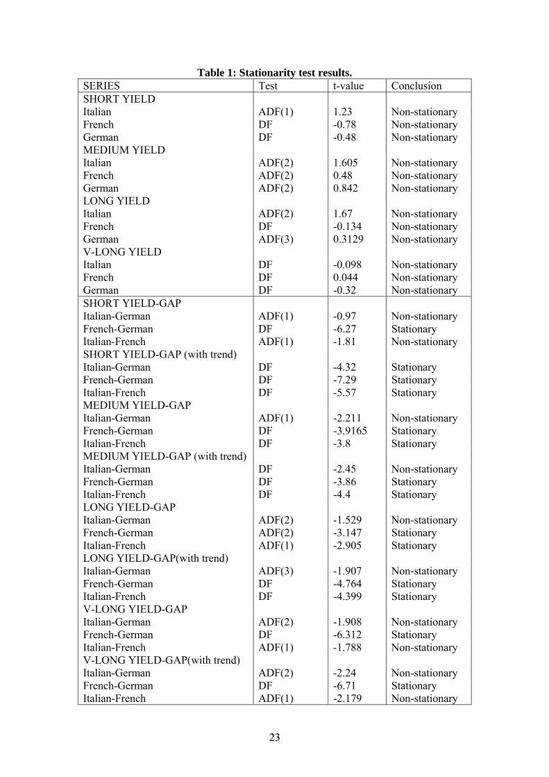
Table 1: Stationarity test results. SERIES Test t-value Conclusion SHORT YIELD Italian ADF(1) 1.23 Non-stationary French DF -0.78 Non-stationary German DF -0.48 Non-stationary MEDIUM YIELD Italian ADF(2) 1.605 Non-stationary French ADF(2) 0.48 Non-stationary German ADF(2) 0.842 Non-stationary LONG YIELD Italian ADF(2) 1.67 Non-stationary French DF -0.134 Non-stationary German ADF(3) 0.3129 Non-stationary V-LONG YIELD Italian DF -0.098 Non-stationary French DF 0.044 Non-stationary German DF -0.32 Non-stationary SHORT YIELD-GAP Italian-German ADF(1) -0.97 Non-stationary French-German DF -6.27 Stationary Italian-French ADF(1) -1.81 Non-stationary SHORT YIELD-GAP (with trend) Italian-German DF -4.32 Stationary French-German DF -7.29 Stationary Italian-French DF -5.57 Stationary MEDIUM YIELD-GAP Italian-German ADF(1) -2.211 Non-stationary French-German DF -3.9165 Stationary Italian-French DF -3.8 Stationary MEDIUM YIELD-GAP (with trend) Italian-German DF -2.45 Non-stationary French-German DF -3.86 Stationary Italian-French DF -4.4 Stationary LONG YIELD-GAP Italian-German ADF(2) -1.529 Non-stationary French-German ADF(2) -3.147 Stationary Italian-French ADF(1) -2.905 Stationary LONG YIELD-GAP(with trend) Italian-German ADF(3) -1.907 Non-stationary French-German DF -4.764 Stationary Italian-French DF -4.399 Stationary V-LONG YIELD-GAP Italian-German ADF(2) -1.908 Non-stationary French-German DF -6.312 Stationary Italian-French ADF(1) -1.788 Non-stationary V-LONG YIELD-GAP(with trend) Italian-German ADF(2) -2.24 Non-stationary French-German DF -6.71 Stationary Italian-French ADF(1) -2.179 Non-stationary

23

Table 2: Cointegration: Short Maturity Johansen Test of Cointegrating Rank. Endogenous Variables: Italian, French and German Yields. Exogenous variables in cointegration space: Drift and trade-type indicators. Unrestricted constant outside cointegration space. Lag length: 1 Effective sample: 2 to 88 Eigenvalues L-max Trace H0: rank L-max Crit. 90% Trace Crit. 90%

0.4276 48.55 75.12 0 16.13 39.08 0.1743 16.66 26.58 1 12.39 22.95 0.1077 9.92 9.92 2 10.56 10.56

Conclusion Both the L-Max and Trace statistics imply that there are two cointegrating vectors. Philips-Hansen pair-wise cointegrating regressions: Standard Deviation of residual for all regression pairings (dependent variable listed first – all regressions include intercept, trend and trade-type dummies)

French-German

German-French

Italian-French

French-Italian

Italian-German

German-Italian

1.23 1.32 1.17 1.28 1.09 1.23 Conclusion. Italian bond provides the benchmark.

Table 3: Cointegration: Medium Maturity

Johansen Test of Cointegrating Rank. Endogenous Variables: Italian, French and German Yields. Exogenous variables in cointegration space: Drift and trade-type indicators. Unrestricted constant outside cointegration space. Lag length: 1 Effective sample: 2 to 88

Eigenvalues L-max Trace H0: rank L-max Crit. 90% Trace Crit. 90% 0.4277 48.55 67.73 0 16.13 39.08 0.139 13.02 19.18 1 12.39 22.95 0.0684 6.16 6.16 2 10.56 10.56

Conclusion L-Max statistic implies 2 cointegrating vectors while Trace statistic implies 1. Philips-Hansen pair-wise cointegrating regressions: Standard Deviation of residual for all regression pairings (dependent variable listed first – all regressions include intercept, trend and trade-type dummies)

French-German

German-French

Italian-French

French-Italian

Italian-German

German-Italian

0.847 0.96 0.97 0.95 1.09 1.11 Conclusion. French bond provides the benchmark.

24

Table 4: Cointegration: Long Maturity Johansen Test of Cointegrating Rank. Endogenous Variables: Italian, French and German Yields. Exogenous variables in cointegration space: Drift and trade-type indicators. Unrestricted constant outside cointegration space. Lag length: 3 Effective sample: 4 to 88 Eigenvalues L-max Trace H0: rank L-max Crit. 90% Trace Crit. 90%

0.3034 30.74 66.43 0 16.13 39.08 0.2829 28.26 35.7 1 12.39 22.95 0.0838 7.44 7.44 2 10.56 10.56

Conclusion Both the L-Max and Trace statistics imply that there are two cointegrating vectors. Philips-Hansen pair-wise cointegrating regressions: Standard Deviation of residual for all regression pairings (dependent variable listed first – all regressions include intercept, trend and trade-type dummies)

French-German

German-French

Italian-French

French-Italian

Italian-German

German-Italian

1.15 1.10 1.29 1.33 0.997 0.983 Conclusion. German bond provides the benchmark.

Table 5: Cointegration: Very-Long Maturity

Johansen Test of Cointegrating Rank. Endogenous Variables: Italian, French and German Yields. Exogenous variables in cointegration space: Drift and trade-type indicators. Unrestricted constant outside cointegration space. Lag length: 1 Effective sample: 2 to 88 Eigenvalues L-max Trace H0: rank L-max Crit. 90% Trace Crit. 90%

0.4064 45.37 70.67 0 16.13 39.08 0.1726 16.48 25.3 1 12.39 22.95 0.0964 8.82 8.82 2 10.56 10.56

Conclusion Both the L-Max and Trace statistics imply that there are two cointegrating vectors. Philips-Hansen pair-wise cointegrating regressions: Standard Deviation of residual for all regression pairings (dependent variable listed first – all regressions include intercept, trend and trade-type dummies)

French-German

German-French

Italian-French

French-Italian

Italian-German

German-Italian

1.00 0.966 1.49 1.59 1.40 1.46 Conclusion. German bond provides the benchmark.

25

Table 6: Coverage of Data Set Country Number

of bonds.

% Number of transactions in All Bonds.

% Transactions in most liquid bond.

%

Short Maturity. German 7 16.7 808 3.7 280 11.9 French 4 9.5 938 4.3 517 22.0 Italian 31 73.8 20151 92.0 1551 66.1 Medium Maturity. German 23 36.5 1358 4.9 407 6.0 French 11 17.5 2048 7.5 606 9.0 Italian 29 46.0 24046 87.6 5744 85.0 Long Maturity. German 20 43.5 2221 6.3 722 3.0 French 15 32.6 2426 6.8 1081 4.5 Italian 11 23.9 30873 86.9 22059 92.4 Very-Long Maturity. German 4 28.6 1127 13.5 679 12.2 French 5 35.7 451 5.4 261 4.7 Italian 5 35.7 6767 81.1 4641 83.2 All Maturities. Total Short 42 25.5 21897 23.5 2348 6.1 Total Medium 63 38.2 27452 29.5 6757 17.5 Total Long 46 27.9 35520 38.1 23862 61.9 Total V-Long 14 8.5 8345 9.0 5581 14.5 Total All 165 100.0 93214 100.0 38548 100.0

26

constant+noisei ir Log v

1 We did in fact carry out Granger-causality tests and the generally inconclusive results are in the web

appendix.

2 In what follows, all variables are implicitly indexed by time. To avoid cluttering the notation, we

suppress the time subscripts.

3 See for example John Cochrane’s 2001 book ‘Asset Pricing’. It has less than two pages devoted to

stationarity.

β= − +

i

4 For example: where v is the velocity of money. The latter is

typically non-stationary. β is the inverse of the interest semi elasticity of the demand for money and

is country specific.

5 This also implies that our model is an unconditional factor model. A conditional factor model can be

re-expressed as an unconditional factor model with additional factors equal to the existing factors

scaled by the conditioning variables. The introduction of a multi-factor model is certainly feasible but

is not indicated by our empirical results. In Section 4, we compare 3 countries. If there were two

nonstationary factors there would be at most one cointegrating vector between the three. If pairwise

cointegration is rejected this amounts to a refutation of the one factor model.

6 For example, for Cobb-Douglas production technology, all that is required is that the capital-output

ratio is trend stationary.

7 A strong restriction is that the constant in both cointegrating vectors be unity. This corresponds to

two stationary yield gaps. The discussion in the next section will show that this is problematic.

8 If residuals from the structural vectors are not orthogonal, then it is not clear what ‘structural’ means

in this context. It is essential one way or the other to make some assumption about the covariance

between the structural relations. However, any assumption other than a zero value makes the

application of the irreducible cointegrating vector approach inconclusive.

2 13 and e e γδ

β β−

= =

1

e9 Note that

β ≤10 The requirement that may appear arbitrary and dependant on normalisation. If the outcome

of a specific analysis is dependant on the choice of normalisation, the theory of the previous section

provides a good guide. Suppose that the Italian bond is proposed as a benchmark. Lemma 2 requires

27

that that all equations, involving this proposed benchmark, should be normalised on the Italian yield.

For the cross-equation, involving the German and Italian bonds, lemma 1 requires that we calculate:

2 2

1 1Var G GF FG F F G

G F G F F G

r r Var r r Var r rβ ββ β β β β β

⎛ ⎞ ⎛ ⎞⎛ ⎞− = − = −⎜ ⎟ ⎜ ⎟⎜ ⎟

⎝ ⎠⎝ ⎠ ⎝ ⎠

F G Gr Fr

In practice, the last two expressions can be interpreted as derived from estimation using the two

possible normalisations i.e. regressing r on r and on respectively. The resulting residual

variances are deflated by 2

1

Gβ2

1

Fβ and .respectively. These can be interpreted as being derived from

regressing the German return on the proposed Italian benchmark ˆGβ ˆ

Fβ and similarly for . The final

step is to compare the three variances. Using the BCH maximum variance criterion, this either

confirms or refutes the supposition that (in this case) the benchmark is the Italian bond.

2 2

ˆ ˆ1 1ˆ ˆ ˆ ˆ

G FG F F G

G F F G

Var r r Var r rβ ββ β β β

⎛ ⎞ ⎛ ⎞− = −⎜ ⎟ ⎜ ⎟⎜ ⎟ ⎜ ⎟

⎝ ⎠ ⎝ ⎠There are two obvious points here. Firstly, is only

correct asymptotically. Consequently, the ranking could be ambiguous: in that case, we could not

conclude that the benchmark is Italian.. For the same reason, two different bonds could be identified as

benchmark: in that case no conclusion about the identity of the benchmark could be reached. This

would occur if benchmark status were contested: this in itself would be an interesting result.

11 The appropriate sample period for a particular study very much depends on the sort of market that

one is considering. In the vector error correction representation of the model a typical value of the

ECM adjustment coefficients is 0.05. Since the data is half daily, this means that the half-life of a

response to a shock to equilibrium is just over 4 days. In such a market two months is a long enough

time-span.

12 Ireland joined Euro-MTS in June 2002.

13 Short-dated bonds have maturities between 1.25 and 3.5 years. Medium, long and very long bonds

have maturity spans of 3.5-6.5 years, 6.6-13.5 years and >13.5 years respectively. There is also a fifth

category for bills: securities with maturity less than 1.25 years. However, until recently, only Italy was

significantly trading such instruments on Euro-MTS. There is also a fifth category for bills: securities

with maturity less than 1.25 years. However, until recently, only Italy was significantly trading such

instruments on Euro-MTS.

28

14 Trading is heavily dominated by the modal trade size. Over 90% of trades for the first three

maturities occur at the mode while 78% are at the mode for the very-long maturity.

15 We use 12.30 as the end of the morning trading period and 4.30 as the end of the afternoon trading

period.

16 More details of these tests can be obtained from the relevant web address listed above.

29