Price and Volatility Spillovers Across the International ...
51
Price and Volatility Spillovers Across the International Steam Coal Market Jonathan A. Batten a , Janusz Brzeszczynski b , Cetin Ciner c , Marco C. K. Lau d , Brian Lucey e,* , Larisa Yarovaya f a School of Economics, Finance and Banking, Universiti Utara Malaysia, Sintok, 06010, Kedah, Malaysia b Newcastle Business School, Northumbria University, Newcastle upon Tyne NE1 8ST, United Kingdom c Cameron Business School, UNC Wilmington, 601 S. College Road, Wilmington NC 28403 USA d Huddersfield Business School, University of Huddersfield, Huddersfield HD1 3HD, United Kingdom e Trinity Business School, Trinity College Dublin, Dublin 2, Ireland & University of Sydney Business School, H70, Abercrombie St & Codrington St, Darlington NSW 2006, Australia & Institute of Business Research, University of Economics Ho Chi Minh City, 59C Nguyen Dinh Chieu, Ward 6, District 3, Ho Chi Minh City, Vietnam f Southampton Business School, University of Southampton, SO17 1BJ, United Kingdom Abstract We examine the degree of integration of the global steam coal market. Using a variety of measures, we show that the Australian market remains the dominant force in setting world coal prices, fol- lowed by Mozambique and South Africa. We find little evidence of asymmetric price and volatility transmission. In fact, most markets react to both positive and negative shocks in a symmetric man- ner. The coal market displays a significant degree of integration, although this effect varies over time. While China provides a major source of volatility to the global coal market, it is relatively insignificant in terms of price transmission. Keywords: Integration; Information transmissions; Generalized VAR model; Steam coal JEL Codes : C32, F18, F49, Q37 * Corresponding Author Email addresses: Email:[email protected] (Jonathan A. Batten), Email:[email protected] (Janusz Brzeszczynski), Email:[email protected] (Cetin Ciner), Email:[email protected] (Marco C. K. Lau), Email:[email protected] (Brian Lucey), Email:[email protected] (Larisa Yarovaya) brought to you by CORE View metadata, citation and similar papers at core.ac.uk provided by Huddersfield Research Portal
Transcript of Price and Volatility Spillovers Across the International ...

Price and Volatility Spillovers Across the International Steam Coal
Market
Jonathan A. Battena, Janusz Brzeszczynskib, Cetin Cinerc, Marco C. K. Laud, BrianLuceye,∗, Larisa Yarovayaf
aSchool of Economics, Finance and Banking, Universiti Utara Malaysia, Sintok, 06010, Kedah, MalaysiabNewcastle Business School, Northumbria University, Newcastle upon Tyne NE1 8ST, United Kingdom
cCameron Business School, UNC Wilmington, 601 S. College Road, Wilmington NC 28403 USAdHuddersfield Business School, University of Huddersfield, Huddersfield HD1 3HD, United Kingdom
eTrinity Business School, Trinity College Dublin, Dublin 2, Ireland &University of Sydney Business School, H70, Abercrombie St & Codrington St, Darlington NSW 2006,
Australia &Institute of Business Research, University of Economics Ho Chi Minh City, 59C Nguyen Dinh Chieu, Ward
6, District 3, Ho Chi Minh City, VietnamfSouthampton Business School, University of Southampton, SO17 1BJ, United Kingdom
Abstract
We examine the degree of integration of the global steam coal market. Using a variety of measures,we show that the Australian market remains the dominant force in setting world coal prices, fol-lowed by Mozambique and South Africa. We find little evidence of asymmetric price and volatilitytransmission. In fact, most markets react to both positive and negative shocks in a symmetric man-ner. The coal market displays a significant degree of integration, although this effect varies overtime. While China provides a major source of volatility to the global coal market, it is relativelyinsignificant in terms of price transmission.
Keywords: Integration; Information transmissions; Generalized VAR model; Steam coal
JEL Codes : C32, F18, F49, Q37
∗Corresponding AuthorEmail addresses: Email:[email protected] (Jonathan A. Batten),
Email:[email protected] (Janusz Brzeszczynski), Email:[email protected](Cetin Ciner), Email:[email protected] (Marco C. K. Lau), Email:[email protected] (Brian Lucey),Email:[email protected] (Larisa Yarovaya)
brought to you by COREView metadata, citation and similar papers at core.ac.uk
provided by Huddersfield Research Portal

1. Introduction
Steam coal (also known as thermal coal) is the most important fuel source for power
generation worldwide. In 2016, for example, coal accounted for 37% of global electricity
production, while the next four largest sources, i.e. gas, renewables, nuclear energy and oil,
represented only 24%, 24%, 11% and 4% of the global market, respectively1. The importance
of coal as an energy source also continues to rise. For example, the demand for steam coal
in generating electricity increased from 33% in 1971 to 41% in 2013 (World Bank., 2015)2.
Thus, despite the increased use of alternative energy sources worldwide, the percentage share
of coal as an energy source has increased relative to its long-term average value.
In this paper we examine the degree of integration of the steam coal market. Many energy
sector analysts and researchers consider the international coal market to be well-integrated
(e.g., (Ellerman, 1995), (Humphreys and Welham, 2000); (Warell, 2006); (Li et al., 2010a);
(Smiech et al., 2016)). While there is little debate on the presence of integration in the
coal market, there is only limited empirical evidence available regarding the intensity and
direction of return and volatility transmission effects across the various regional coal markets,
which historically have been segmented due to distances imposed by particular geographical
locations. Furthermore, the question of asymmetric information transmission across markets,
which is well documented in the finance literature, is still largely unexplored in this area of
energy economics.
The closest contribution to ours has been provided by Papiez and Smiech (2015) who
analysed the integration of the steam coal markets using weekly data spanning from October
5, 2001 to March, 28, 2014. Papiez and Smiech (2015) employed the rolling trace test to
identify the level of coal markets integration. They found the relationships between the
freight costs and degree of integration between markets. Particularly, in the periods when
freight costs are higher the integration is weaker, while in the period when the costs are
lower the integration is stronger. They also identified the main price-setters and price-takers,
highlighting that their roles are changing over time. However, Papiez and Smiech (2015)
1Source: World Coal Association, www.worldcoal.org/global-electricity-mix2This number is based on the authors calculations using data from 169 countries, for the period from 1960
to 2014. It should be noted that there is significant variation between countries. For example, as much as
95% of electricity is generated from coal-fired power plants in Botswana and South Africa, 75% in Australia
and 69% in China. On the other hand, other countries use less coal for their electricity production due to
alternate sources of supply, such as from nuclear power (e.g. in France only 2% of electricity was generated
from coal-fired power plants in 2014). Ninety five percent of electricity is generated from coal-fired power
plants in Botswana and Mozambique, while the figure for China is 69%, and 75% for Australia.
2

study employs only coal prices although the intensity and dynamics of volatility spillovers
can be different from level. Therefore, we augment the existing evidence on information
transmission mechanism between steam coal markets using alternative empirical approaches
that are employed to both prices and volatilities.
Our paper differs from other studies in the literature in the following ways. First, it pro-
vides novel evidence about both the price and volatility transmission processes across eight
major international coal markets. To understand these dynamics, we apply the variance
decomposition framework of Diebold and Yilmaz (2012) to weekly coal prices and volatilities
in order to measure the total, directional and net-pairwise spillover indices. Second, we also
use an asymmetric causality test of Hatemi-J (2011) to provide new results on the degree
of asymmetry in the spillovers present in the global coal market. We augment them with a
number of additional robustness tests. These statistical measures show that the Australian
market remains the dominant force in setting world coal prices with little evidence of asym-
metric price and volatility transmission. Consistent with previous findings, we show that
the international coal market displays a significant degree of integration, although this effect
varies over time due to different economic shocks and other impacts arising from technological
innovation.
Finally, we provide indication regarding how our results can be used for the design of
hypothetical trading strategies relying on the findings about the markets which have been
identified as net-contributors and net-recipients.
The paper is organized as follows. The next Section 2 provides the overview of the steam
coal market. Section 3 presents a review of the literature about integration and spillover
effects in the coal market. Section 4 describes the dataset and the methodology used in our
empirical analysis, while Section 5 reports the empirical results. Section 6 provides indication
regarding how our findings can be used for the design of hypothetical trading strategies.
Section 7 discusses the results and presents their broader economic interpretations as well as
implications for international steam coal market participants. Finally, Section 8 concludes
the paper.
2. Steam Coal Market Overview
Globalization and other economic and political drivers of the integration process in the
coal industry began in the 1960s. Until that time, the international coal market was highly
fragmented with mostly domestic production of steam coal used by households for heating.
Coal was rarely exported due to high transportation costs. With significant increases in
3

the oil price, following the Organization of Arab Petroleum Exporting Countries (OAPEC)
oil embargo in the 1970s, the demand for steam coal for electricity generation increased
signifiantly. Improvements in transport infrastructure also occurred around this timewith
the cost of shipping declining significantly (Lundgren, 1996). All tese factors drove the
increase in global demand for coal, during the period of four decades between 1965 and 2014,
by more than 278% (British Petroleum, 2015).
The two largest coal producing countries worldwide are China (1844.6 Mt Million tonnes
oil equivalent in 2014) and the United States (507.8 Mt Million tonnes oil equivalent in
2014), although these two markets mainly consume their own coal. The major coal exporting
countries are Australia, Indonesia, Columbia and South Africa, while a number of other key
countries have limited domestic production and rely on coal imports. These markets include
the key industrialised export-based economies of Japan, South Korea and Taiwan as well as
some western European countries.
International trading activity in coal is clearly divided into two geographical centres based
around the Atlantic and Pacific regions. The trade pattern within these two regions is based
on variation in domestic production and freight costs (Warell (2006)). The Atlantic market
includes Northwest Europe, South Africa, Colombia and Russia, where Russia is the largest
exporter. The cost, insurance and freight (cif) ARA price (Amsterdam, Rotterdam, Antwerp)
is the benchmark coal price for European importers in the Atlantic basin market, while free
on board (fob), meaning that the buyer takes delivery of shipped goods once the goods leave
the supplier’s shipping dock, is used elsewhere. For example, key export prices are fob Puerto
Bolivar (Colombia), fob Richards Bay (South Africa) and fob Baltic ports (Russia). Papiez
and Smiech (2015) found that price movements appear to be initiated mainly by the Atlantic
market with pricing from the ARA ports being of particular importance.
Within the Pacific market the largest importing countries are Japan, South Korea, China,
Taiwan and India, whereas Australia, Indonesia, Vietnam, China and Russia are the main
exporters. While India is technically not located on the Pacific rim, its suppliers however
are. South Africa is uniquely placed geographically to supply both the Atlantic and Pacific
basin markets. The main benchmark importing price is cif South China, while the main
benchmark exporting price in the Pacific market is fob Newcastle-Australia (Zaklan et al.
(2012b) and Papiez and Smiech (2015)).
4

3. Integration and Spillovers in Coal Market
The existence of an integrated commodity market is implied through the economic theory
of the law of one price. Originally, Heckscher (1916) argued that trade-based transaction
costs, arising from spatial separation of counter-parties, can lead to deviations from the law
of one price (i.e. price divergence). The basic research framework for analysis of non-linear
price convergence is presented in Section 3. This investigation is motivated by a number
of papers including Taylor et al. (2001); Sarno et al. (2004) and Apergis and Lau (2015).
The price differential creates an arbitrage opportunity for the same, and to some extent
substitutable, good (e.g. steam coal of various qualities). Thus, lower-priced goods will be
transported to another region and sold for a higher price (inclusive of all transaction and
transportation costs). In equilibrium, the prices of the same good at different locations will
converge to a single price (or at least to a similar price level).
Note that within this framework, the trade only occurs on condition that price difference,
or profit, generated from the arbitrage activities can cover the transaction cost (see Taylor
et al. (2001)). For example, consider a case where Australia ships steam coal to Europe and
Japan. If the law of one price holds, the price differential between Europe and Japan should
be equal to the difference in shipping costs between Australia-Europe and Australia-Japan
Warell (2006).
Numerous empirical studies have applied the theoretical non-linear version of the law of
one price to allow for differences in the degree of income and price convergence (for example,
see Akhmedjonov et al. (2013); Lau et al. (2012); Akhmedjonov and Lau (2012); Lau et al.
(2012); Suvankulov et al. (2012)). Other notable recent studies include Akhmedjonov et al.
(2013), who uses Exponential Smooth Auto Regressive Augmented DickeyFuller (ESTAR-
ADF) unit root tests to investigate the unconditional income convergence across Russian
regions, and finds evidence of inter-regional inequalities. Another example is Lau et al.
(2012), who propose a new theoretical model to investigate if there is income convergence
across the provinces of China. Their study applies a non-linear panel unit root test of
Exponential Smooth Auto-Regressive Augmented Dickey-Fuller (ESTAR-ADF) unit root
test to empirically test the conditional convergence hypothesis in China from 1952 to 2003
and find that the number of converging provinces decreases in the post-reform period.
A similar approach is adopted by Akhmedjonov and Lau (2012), who investigate the
pattern of price convergence in Russian energy markets, comprising diesel, gasoline, electricity
and coal, from January 2003 to October 2010, over 83 Russian regions. Given the geographical
scale of Russia, and variation in transport and infrastructure costs, it is not surprising that
5

they find evidence of segmentation. Nonetheless, the unequal distribution of energy reserves
and limited cross-border transmission capacity across different regions, creates a complex set
of pricing distortions, with the coal price correctly converging in only 37% of the Russian
regions.
However, another obstacle to regional convergence is local protectionism. For example,
Young (2000) argues that there is increasing local protectionism in China, as provinces at-
tempt economic adjustment driven by national policy change (e.g. the decision not to use
local coal that may be more polluting than imported coal).
Market structure is another factor that affects the degree of market integration. (Warell,
2006) suggests that since the coal industry has experienced a number of mergers and ac-
quisitions, this in turn may lead to larger and more monopolistic corporations being able
to manipulate and control prices (Regibeau, 2000). Mergers and acquisitions may result in
barriers to entry, price discrimination and collusion; therefore price convergence across mar-
kets is invalid because the law of one price does not hold. However one may also argue that
mergers and acquisitions drive productivity improvement in the form of cost-cutting, and
this potential increase in profit may encourage price convergence.
Market structure is another factor that affects the degree of market integration. Warell
(2006) suggests that since the coal industry has experienced a number of mergers and acquisi-
tions (see e.g. Regibeau (2000), among others), the establishment of these larger corporations
may lead to less competition in the global market. Given the scale and scope economies avail-
able to these large, merged corporations, this may also lead to infrastructure based barriers
to entry, price discrimination and collusion. Therefore, the conclusion on price convergence
across markets is biased, and potentially misleading in terms of policy outcomes, because the
law of one price does not hold. However, one may also argue that mergers and acquisitions
drive productivity improvement in the form of cost-cutting and that this increase in profit
margin may encourage price convergence.
The existing empirical evidence concerning the scope (and to some extent scale) of coal
market integration is somewhat mixed. Li et al. (2010a) performed a cointegration analysis
using monthly FOB coal prices in the period January 1995 - July 2007 and concludes that
the global steam coal market is well integrated. However, Zaklan et al. (2012a) applied a
similar cointegration analysis to the steam coal market using export and import steam coal
prices, and freight rates for the period December 2001 to August 2009, and find that the
steam coal market is not fully integrated. The analysis by Warell (2006) of the international
coal market, also found evidence of integration between Europe and Japan, for the period
6

1980 to 2000, using cointegration techniques.
Warell (2006) also tested for the presence of a single international market for the steam
coal industry and concluded that there was no long-run cointegrating relationship between
the respective price series (i.e. quarterly Cost, Insurance and Freight (CIF) import coal
prices). The lack of a single market was attributed to mergers and acquisitions during the
sample period. Smiech et al. (2016) investigated the relationships between steam coal prices
in the Atlantic and Pacific basins using Granger causality tests. They concluded that the
Pacific basin plays a dominant role in the setting of global price due to the large import
demand from China, Korea and Japan.
We contribute to the energy economics literature by undertaking a more extensive analysis
of the global coal market than these previous studies. Our findings reveal complex patterns
of price and volatility transmission mechanisms within the global coal market. Moreover, we
consider not only regional price causality, but also examine the spillover and transmission
channels of price and volatility across markets using the Diebold and Yilmaz (2012) frame-
work. This method has been previously employed in analysis of the interrelationships in the
global base metal markets by Ciner (2018) and spillovers between equity and futures markets
by Yarovaya et al. (2016), but to our best knowledge it has not been applied to the steam
coal markets yet. Thus, a key novelty of this paper is that it is the first study to provide an
empirical analysis of price and volatility spillovers and transmission mechanisms across the
international coal market using this new methodology.
4. Methodology
4.1. Data
Our study employs weekly coal price index data from January 12, 2001 to December
26, 2014. We investigate price convergence and spillover effects across eight international
steam coal markets located in Australia, China, Amsterdam Rotterdam Antwerp, Colombia,
Russia (Baltic), Russia (Vostochny), Mozambique, and South Africa. All data are sourced
from Bloomberg. Table 1 presents the summary statistics of the stem coal prices in these
eight steam coal markets. Sample means, medians, maximums, minimums, standard devi-
ations, skewness, kurtosis, and the Jarque-Bera (JB) statistic are reported. According to
key statistics on the supply, transformation and consumption of all major energy resourcers
provided by the International Energy Agency, the leading producers of coal are China, Aus-
tralia, Russia and South Africa accounted for 44.7%, 6.6%, 5.1% and 3.4% of world total coal
production in 201, respectively. It is also important to highlight that the net exporters of coal
7

are Australia (379Mt), Russia (161Mt), South Africa (71Mt) and Mozambique (12Mt), while
China (263Mt) is still net importer of coal regardless its leading role in the global production
of coal3.
The weekly price indexes for the markets ranged from $64.538 (South Africa) to $81.056
(China). The standard deviations range from $28.027 (Europe) to $41.213 (China). China is
the most volatile market while Europe is the most stable market. There are also some types
of nonlinear components within its Data Generating Process (DGP). Table 1 also shows a
clear evidence of departures from normality (as implied by significant JB statistics).
Table 3 reports tests for the presence of a unit root (we accept the null hypothesis of a
unit root at the 0.01 level of significance). We conclude that the steam coal price indexes are
non-stationary. The test also indicates that a structural break occurs in late 2007 with the
exception of China and the Russian Baltic. Moreover we use the Narayan et al. (2010) 2-break
test, which is more powerful. The result shows that all series contain a unit root, with an
exception of Australian market (see Table 4, panel A). Furthermore, because the empirical
analysis is based on weekly data, Narayan and Liu (2015) show that heteroskedasticity is
an issue and therefore they develop a GARCH unit root test. As data actually exhibit
heteroskedasticity, we therefore carried out the test of Narayan and Liu (2015), and the
result shows that all series are stationary (see Table 4, panel B).
4.2. Nonlinear Panel Unit Root Test
Numerous studies apply unit root tests to investigate market integration. For example,
Fan and Wei (2006) find evidence of high integration between major Chinese goods, such
as raw materials and durable goods; Ma et al. (2009) provide evidence that major energy
prices are converging to their national averages in China; Suvankulov et al. (2012) investigate
gasoline price convergence in Canada using nonlinear panel unit root test and find evidence
that price convergence has declined significantly since July 2006; Fallahi and Voia (2015)
study the stochastic convergence of per capita energy use in 25 OECD countries; Presno
et al. (2014) find evidence of convergence in per capita CO2 emissions in 28 OECD countries
using nonlinear unit root test.
The use of a nonlinear panel unit root test can achieve higher statistical power in com-
parison to a linear panel unit test if data contains non-linear elements (Lau et al., 2012) and
this fact is confirmed here by the BDS test. Consider the series of interest for market i, which
3Source: www.iea.org/statistics/kwes/supply/
8

at time t is y(i, t) that is defined as follows:
yi,t = ln(Vi,t
Vt) (1)
where Vi,t is the price index for market i at time t (t = 1...T ); yi,t is the relative price index
in comparison to the average, and Vt is the average price index across all markets at time
t. Following Cerrato et al. (2011, 2013), the Data Generating Process (DGP) for the time
series of interest yi,t, can be modelled as:
yi,t = ξiyi,t−1 + ξ∗i yi,t−1Z(θi; yi,t−d) + µi,t (2)
where
Z(θi; yi,t−d) = 1− exp[−θi(yi,t−d − χ∗)2] (3)
and θi is a positive parameter and χ∗ is the equilibrium value of yi,t (i.e. the equilibrium price
differential between two markets). It is important to note that this value of χ∗ quantifies the
abstract idea of transaction cost (inclusion of shipping costs, storing costs; inland transport
costs, loading cost and unobserved hidden costs originated from heterogeneous institutional
arrangements for different locations); µi,t is the error term and it has a one-factor structure
such as:
µi,t = γift + εi,t (4)
(εi,t)t ∼ i.i.d.(0, σ2i ) (5)
where ft is the unobserved common factor and εi,t is the individual-specific (idiosyncratic)
error. Following the literature, we set the delay parameter d to unity such that Equation (5)
in its first difference yields:
∆yi,t = αi + ξiyi,t−1 +h−1∑h=1
δijh∆yij,t−h + (α∗i + ξ∗i yi,t−1+
h−1∑h=1
δ∗ih∆yij,t−h)∗Z(θi; yi,t−d) + γif + i+ εi,t (6)
Several characteristics of Equation (6) are noteworthy:
a) When yi,t−d = c, Z(.) = 0 the equation converges to the linear augmented Dickey-Fuller
model.
b) When the price difference between two markets is far from its equilibrium level4 it
4Literally, the term equilibrium means at this level of price differential that the market i has no incentive
to change its current exporting price after taking into consideration all of the transaction costs and potential
profit.
9

implies the differential between yi,t−d (i.e. the actual coal price difference d lagged periods)
and χ is too large, a new linear augmented Dickey-Fuller model with parameter βi = ξi + ξ∗i
in Equation (2) will emerge immediately because Z(.)will approach 1.
c) As the gap between the actual and equilibrium level of the coal price difference between
the two markets is negligible, the parameter ξ∗i is responsible for the movement of yi,t. Or, if
the gap between the actual and equilibrium level of the price difference is too large, ξ∗i will
dominate the adjustment process of the relative coal price in Equation (2).
d) As discussed in the literature, ξi + ξ∗i < 0 is the necessary condition for global stability
to hold. As long as ξi + ξ∗i < 0 holds in the adjustment process, ξ∗i ≥ 0 can exist.
e) yi,t may follow a non-stationary process (e.g. a random walk or possibly an explosive
innovation within the band of inaction of ξ∗) and it will converge to its equilibrium level
when the magnitude of price divergence is outside the ”band”.
Once we assert that yi,t follows a unit root process in the middle regime of ξi = 0, the
Equation (5) can be rewritten as:
∆yi,t = ξ∗i yi,t−1[1− exp(−θiy2i,t−1)] + γift + εi,t (7)
We can form the null hypothesis of non-stationarity H0 : θi = 0∀i against its alternative
H1 : θi > 0 for i = 1, 2, ..., N1 and θi = 0 for i = N1 + 1, ..., N . Due to the fact that ξ∗i is
not identified under the null hypothesis, the null hypothesis cannot be tested. Cerrato et al.
(2011) use a first-order Taylor series approximation method that reparametrizes Equation
(7) and the auxiliary regression yields:
∆yi,t = ai + δy3i,t−1 + γift + εi,t (8)
Equation (8) can be extended if errors are serially correlated becoming:
∆yi,t = ai + δy3i,t−1 +
h−1∑h=1
ϑi,h∆yi,t−h + γift + εi,t (9)
Cerrato et al. (2011) further prove that the common factor ft can be approximated by:
ft ≈1
γ∆yt −
b
γy3t−1 (10)
where yt is the mean of yi,t and b = 1N
∑Ni=1 bi. Combining Equation (9) and Equation
(10), it can be written as the following non-linear cross-sectionally augmented DF (NCADF)
regression:
∆yi,t = ai + biy3i,t−1 + ci∆yt + di∆y
3t−1 + εi,t (11)
10

t-statistics can be derived from bi, which are denoted by:
tiNL(N, T ) =bi
s.e.(bi)(12)
where bi is the OLS estimate of bi, and s.e.(bi) is its associated standard error. The t-statistic
in Equation (12) can be used to construct a panel unit root test by averaging the individual
test statistics:
tiNL(N, T ) =1
N
N∑i=1
tiNL(N, T ) (13)
This is a non-linear cross-sectionally augmented version of the IPS test (NCIPS).
4.3. Spillover Index
This study also employs the Diebold and Yilmaz (2012) (DY) framework to measure the
price dynamics and the intensity of information transmission across global coal markets. The
DY framework is based on a generalized vector autoregressive (VAR) model and has been
actively employed in the finance literature to investigate spillover effects across various finan-
cial markets (Diebold and Yilmaz (2009); Batten et al. (2014); Yarovaya and Lau (2016)).
However, to the best of our knowledge, this methodology has not yet been applied to coal
data or to the analysis of coal markets.
The spillover index approach allows presentation of the empirical results in the form of
spillover tables and spillover plots, visualizing the channels and the dynamics of information
transmission across markets. Furthermore, the DY framework can provide a clear evidence
of net-contributors and net-recipients of information in the international coal market. The
DY framework can be described as follows.
Consider a covariance stationary N-variable VAR (p), Xt =∑p
i=1 = ΨiXt−i+εt, where Ψi
is a paremeter matrix, and ε ∼ (0; Σ) is a vector of independently and identically distributed
disturbances. The VAR model can be transformed into a moving average (MA) representa-
tion, Xt =∑∞
i=oAiεt−i, where Ai is ans N × N identity matrix Ai = Ψ1Ai−1 + Ψ2Ai−2 +
...ΨpAi−p beign an N × N identity matrix and with Ai = 0 for i < 0. The DY framework
relies on the N-variable VAR variance decompositions that allows for each variable Xi to be
added to the shares of its H-step-ahead error forecasting variance, associated with shocks
of relevance to variable Xj (where ∀i 6= j for each observation). This provides evidence on
the information spillovers from one market to another. Besides detecting the cross variance
shares, the DY framework defines own variance shares as the fraction of the H-step ahead
error variance in predicting Xi due to shocks in Xi. Following Diebold and Yilmaz (2012),
11

the methodological framework employed in this paper relies on KPPS H-step-ahead forecast
errors, which are invariant to the ordering of the variables in comparison to the alternative
identification schemes like that based on Cholesky factorization (Diebold and Yilmaz (2009))
and can be defined for H = [1, 2...+∞), as:
ϑgij(H) =σ−1jj
∑H−1h=0 (e
′iAhΩej)
2∑H−1h−0 (e
′jAhΩA
′hei)
(14)
where Ω is the variance matrix for the error vector ε; σjj is the standard deviation of the error
term for the jth equation; ei is the selection vector, with one as the ith element and zero
otherwise. The sum of the elements in each row of the variance decomposition∑N
j=1 ϑgij(H)
is not equal to 1. The normalization of each entry of the variance decomposition matrix by
the row sum can be defined as:
ϑgij(H) =ϑgij(H)∑Nj=1 ϑ
gij(H)
(15)
where∑N
j=1 ϑgij(H) = 1 and
∑Ni,j=1 ϑ
gij(H) = N .
The total volatility contributions from KPPS variance decompositions are used to calcu-
late the Total Spillover Index (TSI):
TSI(H) =
∑Ni,j=1,i 6=j ϑ
gij(H)∑N
i,j=1 ϑgij(H)
× 100 =
∑Ni,j=1,i 6=j ϑ
gij(H)
N× 100 (16)
We also estimate Directional Spillover Indices (DSI) to measure spillovers from market i
to all markets j, as well as the reverse direction of transmission from all markets j to market
i, using equations (4) and (5), respectively:
DSIj←i(H) =
∑Ni,j=1,i 6=j ϑ
gji(H)∑N
i,j=1 ϑgij(H)
× 100 (17)
DSIi←j(H) =
∑Ni,j=1,i 6=j ϑ
gij(H)∑N
i,j=1 ϑgij(H)
× 100 (18)
Finally, we explore who are the net-contributors and net-recipients of information in the
international coal market, using the Net Spillover Index (NSI) calculated as the difference
between total shocks transmitted from market i to all markets j and those transmitted to
market i from all markets j:
NSIij(H) =
∑Ni,j=1,i 6=j ϑ
gji(H)∑N
i,j=1 ϑgij(H)
−∑N
i,j=1,i 6=j ϑgij(H)∑N
i,j=1 ϑgij(H)
× 100 (19)
12

4.4. Asymmetric Causality
The asymmetry in causal linkages between international coal prices is assessed using
the asymmetric causality test by Hatemi-J (2011) and the suggested bootstrap simulation
technique for calculating critical values. The approach to transform the data into both
cumulative positive and negative innovations was introduced by Granger and Yoon (2002)
to test time-series for cointegration and it later has been adopted by Hatemi-J (2011). In
effect, we examine whether or not a series negative, or positive, innovations shows greater
causal impact on other series negative, or positive, innovations.
Assume that two integrated variables y1t and y2t are described by the following random
walk processes:
y1t = y1t−1 + θ1t = y1,0 +t∑i=1
θ+1i +
t∑i=1
θ−1i, (20)
and similarly
y2t = y2t−1 + θ2t = y2,0 +t∑i=1
θ+2i +
t∑i=1
θ−2i. (21)
The cumulative sums of positive and negative shocks of each underlying variable can be
defined as follows:
y+1t =
t∑i=1
θ+1i, y
−1t =
t∑i=1
θ−1i, y+2t =
t∑i=1
θ+2i, y
−2t =
t∑i=1
θ−2i, (22)
where positive and negative shocks are defined as: θ+1t = max(∆θ1i, 0); θ+
2t = max(∆θ2i, 0);
θ−1t = min(∆θ1i, 0); θ−2t = min(∆θ2i, 0).
To test the causalities between these components, a vector autoregressive model of order
p, VAR (p) is used:
y+t = v + A1y
+t−1 + ...+ Apy
+t−1 + u+
t , (23)
where y+t = (y1t
+, y2t+) is the 2×1 vector of the variables, v is the 2×1 vector of intercepts,
and u+t is a 2 × 1 vector of error terms (corresponding to each of the variables representing
the cumulative sum of positive shocks); Aj is a 2 × 1 matrix of parameters for lag order
γ(γ = 1, , p). The information criterion proposed by Hatemi-J (2003) is used to select the
optimal lag order (p):
HJC = ln(|Ωj|) + j(n2 lnT + 2n2 ln(lnT )
2T), (24)
where j = 0, ..., p; |Ωj| is the determinant of the estimated variance-covariance matrix of the
error terms in the VAR model based on the lag order j, n is the number of equations in the
VAR model and T is the number of observations.
13

This information criterion was proposed by Hatemi-j (2008). The simulation experiments
confirmed the robustness of this criterion to ARCH effects, which is important in case of
our study due to the existence of heteroskedasticity in the data. The next step of the
analysis is to test the Null Hypothesis that the kth element of y+t does not Granger-cause
the ωth element of y+t using the Wald test methodology. Furthermore, Hatemi-J (2012)
employs a bootstrap algorithm with leverage correction to calculate the critical values for
the asymmetric causality test in order to remedy the heteroskedasticity problem. The details
of the Wald test methodology and the bootstrap procedure are discussed in depth by Hacker
and Hatemi-J (2012).
5. Empirical Results
5.1. Cointegration and Long Term Linkages
As mentioned earlier, the primary purpose of this paper is to identify spillovers and causal-
ity effects between the international coal markets rather than examining their cointegration
properties, which was thoroughly analyzed in (Papiez and Smiech, 2015). However, since our
data covers a longer time period and, also, since we include China in our analysis, we begin
by providing updated evidence on the cointegration of international coal prices and report
the results in Table 2. We also examine the drivers of the system of the coal prices to provide
information on the long term spillovers.
We first test for the cointegration rank of the system. Similar to Papiez and Smiech (2015)
we rely on the full information maximum likelihood method of (Johansen et al., 2000). Since
the econometric details of this approach are commonly known, we do not discuss them in
this study. However, it should be mentioned that in Johansens method, an important issue
prior to conducting the rank tests, is to establish how to deal with any trend in the system,
i.e. specifically whether the trend should enter only in the cointegration relation (Johansens
Case 2) or whether the trend should be orthogonal to the relation (Johansens Case 3). There
is no clear trend in the coal price series, which suggests adopting Case 2. However, we also
test this restriction by means of a likelihood ratio test and the null hypothesis of restricting
the trend cannot be rejected.
The second issue is related to the fact that there is a structural break in the system, as we
detect in this study, during the Global Financial Crisis. Structural breaks could significantly
impact the conclusions of the Johansen (1991) cointegration analysis. In fact, Papiez and
Smiech (2015) state this as one of their primary reasons for conducting rolling tests, since
the full sample analysis could be unreliable. While there is definitely merit in such approach,
14

it should also be mentioned that Johansen et al. (2000) and Lutkepohl et al. (2004) discuss
how the method can be adjusted in the presence of a structural break.
Therefore, in this paper, we follow the (Johansen et al., 2000) method of analysis, to
estimate the p-values for the likelihood ratio (trace) tests to test for cointegration by using
the structural break date identified in the paper on September 14, 2007.
Panel A in Table 2 reveals noteworthy findings. First, we detect five cointegration relations
in the system. This is consistent with our intuition that in the long term international coal
prices will not drift apart arbitrarily from each other. The number of the relations is also
largely consistent with the evidence presented in Papiez and Smiech (2015), although the
analyses is not directly comparable for the reasons mentioned above. However, also note
that we do not find seven cointegration relations, which would indicate perfect convergence
between the international coal prices and, hence, the presence of the law of one price.
In Panel B of Table 2, we report loading coefficients for the coal markets for each of the
cointegration relations. Loading, or speed of adjustment, shows the statistical significance
of the response of each of the coal markets when the system moves away from equilibria.
The purpose of this analysis is to identify which market adjusts least to any disequilibria,
since this one would be the market that drives the long term trend. The loading coefficients
for Australia are never significant, which indicates again that Australia does not respond to
disequilibria. In turn, all of the other markets show significant adjustment to changes in the
cointegration vectors. In other words, they correct for the errors in the system.
In Panel C of Table 2, the focus is on the forecast error variance decompositions (FEVDs)
of the system of equations. The FEVDs provide information on how much of the variables
movements are explained by the past movements of another variable. Since the purpose in
this section is to provide evidence on long term relations, we calculate the FEVDs for 26 and
52 week horizons. We argue that Australia appears to be driving the long term trend in the
system.
If that contention is correct, we should find that the Australian coal price has noticeable
explanatory power for the other prices at these horizons. The results are highly consistent
with this argument. Specifically, after 52 weeks, Australia’s own information explains almost
90 percent of its own movements. In other words, the influence of the other markets on the
price changes in Australia is very limited, as we would expect in the case of the leader of the
system. On the other hand, Australia has significant explanatory power for all of the other
markets in the system. This is again consistent with our contention. For example, after 52
weeks, 73 percent and 70 percent of price changes in COBA and SAMA, respectively, are
15

explained by Australia.
5.2. Market Integration: Nonlinear Panel Unit Root Test
Having found a break in the market on September 14, 2007 we now examine the degree
of market integration pre and post this break. The findings of the nonlinear panel unit root
test indicate that most markets were converging to the mean price index before 2007 with
the exception of two Russian markets and the Australian market (see the left panel of Table
5). However, after the break only the American market and the European market diverge
from the mean (see the left panel of Table 3).
5.3. Return and Volatility Spillovers Across Market
The empirical results of the DY spillover tests are reported in Table 6 for the coal prices
and Table 7 for volatility. The findings indicate that the Total Spillover Index for the market
is 73 %. This implies a well-integrated international market with 73% of the variation in the
market price originating within it. Table 6 also displays values of the net-spillover indices
for each individual market, and indicates the net-contributors and net-recipients of coal price
spillovers.
The contribution of the Australian market to other markets is 210.85 %, which is the
highest in the sample5, whereas Australia contributes 39.4% of spillover indexes to South
Africa. In contrast, Colombia only transmits 5% to the other markets, while China receives
the most price spillovers from the other markets (i.e. 84.13 %), which makes it the largest
net-recipient of price spillover in the global market. In summary, Australia and Mozambique
are the net-contributors of the coal price spillover index, while the net-recipients are China,
Colombia, Europe, Baltic, Russian Vostochny, and South Africa.
We define price volatility as the absolute return6: Vt = |ln(Pt) − ln(Pt−1)|, where Pt
is the weekly closing price of the coal price on day t. Table 7 shows the Total Volatility
Spillover Index for the coal price (i.e., 51.5%), which is appropriately 21.5% lower than the
price spillover. However, we still see that in general over half the volatility in the world
coal market is internally generated. In particular, the contribution of China, in terms of
volatility spillovers, turns out to be the highest (i.e. 79.14%), while it contributes 17.05% to
Europe. Colombia transmits only 26.24% to other countries, while Europe receives 62.38%
5Australia exports 90% of its coal output. Australia is the world’s second biggest net exporter of coal in
2017, and the total amount of coal exports was 379Mt in 2017.6This same calculation is used by recent studies including Forsberg and Ghysels (2007), Antonakakis and
Kizys (2015), and Wang et al. (2016).
16

of volatility spillovers from other countries. Overall, Australia, Europe, Baltic, Mozambique
and China are the net-contributors of price volatility, while the net-recipients are Colombia,
Vostochny and South Africa.
Fig 1 shows the dynamics of the coal price spillovers in the international market using a
60 weeks rolling window. Fig 1 indicates time-varying dynamics for the total price spillovers
indices. We note a clear, but gradually increasing, trend of international coal market total
spillovers over the period April 2005 to September 2007. This is most likely due to a relatively
competitive steam coal market from 2005 to 2008 and there is evidence that steam coal prices
were driven by fundamentally marginal cost (i.e. mining cost escalation and freight rates)
based from 2005 to 2008 ((Truby et al., 2010)). However, the degree of connectedness,
starting from September 2008, decreases as the global financial crisis worsened. Figure 2
presents a similar analysis for volatility. It depicts a solid increase in the within system
volatility spillover that mirrors the decline in the price spillover with the system settling at
a more or less steady state after 2007.
5.4. Time-Frequency Decomposition of International Coal Market Prices Connectedness
We now further investigate the degree of time variation in the system using the spectral
representation of GFEVD as derived in Barunik and Krehlik (2015). It is possible to define
an aggregate measure of the frequency band d specified as7:
Cd = Cd · SW (d) (25)
where the spectral weight SW (d) =∑k
i,j=1(θd)i,j∑i,j(θ)i,j
=∑k
i,j=1(θd)i,j
kis the contribution of frequency
band d to the whole VAR system, and Cd is the total connectedness measure on the con-
nectedness tables (θd) corresponding to an arbitrary frequency of band d. It is important
to note that the total connectedness measures (C) as defined in (Diebold and Yilmaz, 2012)
can be calculated as C =∑
d Cd. The time-frequency dynamics of connectedness can be
obtained by using the spectral representations of variance with moving window of 200 trad-
ing weeks. We use two lags to capture the dynamics in the window. The time-frequency
decomposition of price connectedness is presented in Table 8. With weekly data we then
have 1-5 weeks, 5-20 weeks, 20-60 weeks and 60-200 weeks as the time spectrum8. We set
7For detailed derivation of the GFEVD and explanation of the proposed time-frequency dynamics of
connectedness measures, please refer to page 29 Barunik and Krehlik (2015).8In the R script we set bounds < −c(pi + 0.0001, pi/c(4, 12, 48), 0) such that we have weekly, monthly,
quarterly and yearly cycles. Literally we are investigating time domain on 1-5 weeks, 5-20 weeks, 20-60 weeks,
and 60-200 weeks.
17

the H steps forecast horizon to be 100 as an approximation of the frequencies (especially
for low frequencies around zero this choice is appropriate). As we take a Fourier transform
of the impulse response functions, we therefore need larger forecast horizons to obtain low
frequencies.
In a similar analysis, Greenwood-Nimmo et al. (2015) notes that with increasing horizon,
directional connectedness intensies, and rapidly converges to a long-run value. While this
is attributed to gradual transmission of shocks, we add that this behaviour is also perhaps
due to a long frequency response of the shocks. Increasing the horizon will then only better
approximate the permanent effects of shocks. Moreover, the nature of the shocks will not
allow isolation of the connectedness at business cycle frequencies, as discussed earlier. Here,
using frequency responses of shocks and our spectral representation of measures will be useful.
Table 8 shows the connectedness at different cycle frequencies and it reveals how the system
was connected in these cycles.
We find that the largest connectedness comes from frequencies higher than yearly cycles
(i.e. 60-200 weeks) with a value of 80.1, while the weekly, monthly and quarterly cycles are
connected with values of 0.3, 0.7 and 2.6, respectively. Previous studies use aggregate effects
to measure market connectedness by applying methods of causality testing, systemic risk,
co-movement and spillovers index. but they emphasize the empirical importance of frequency
sources of connectedness, arguing that shocks to volatility will impact differently on future
uncertainty 9.
More generally, Table 8 reinforces the importance of Australia at all frequencies, as the
main source of price contribution, which is followed by South Africa albeit at a lower level.
Columbia, at the shorter frequency, is also an important net-contributor. Indeed, at the
shorter cycles, it is Columbia that tends to be the largest gross (but not net) contributor. This
is consistent with a segmented market both in terms of geography and time. Furthermore,
the Australian market receives the highest spillover index (i.e. at 60-200 weeks frequency)
from South Africa and Russia Vostochny has the lowest connectedness with the Baltic. The
decomposition shows that the largest portion of connections is created from lower frequencies
of 60 weeks up to 200 weeks and higher frequencies up to one month play an insignificant
role in the degree of connectedness. Our results also provide important insights into the time
dynamics of the frequency connections since there is a clear pattern of lower frequency bands
9Changes in mining cost escalation and freight rates may trigger fundamental changes in investors expec-
tations, and this shock will impact the market in the longer term. These long-term expectations may transit
to surrounding coal markets in the portfolio differently than shocks that have a short-term impact.
18
dominating all others, whereas connectedness has been driven mostly by yearly information.
5.5. Asymmetry in Price Spillovers
Finally, we analyse how positive and negative innovations on one market affect positive
and negative innovations in another market. Table 9 reports the results of the application of
the asymmetric causality test by Hatemi-J (2011) to coal prices. The results are organized
by presenting them for each market as a contributor of information.
Table 9 shows that for majority of market pairs an asymmetry in spillover effect is not ev-
ident, i.e. the transmission of both negative and positive innovations is equally pronounced.
It is clearly visible, for example, for China, Europe and the South Africa markets (Panel B, C
and G). However, there are a few notable exceptions. A decline in coal prices in the Colom-
bian market causes a decline in prices in the Australian, Vostochny, Baltic, South Africa and
Mozambique markets, while an increase in prices in the same Colombia market causes only
an increase in the Baltic market. This indicates that the transmission of negative shocks
from this market is stronger than the transmission of positive shocks. Similar patterns of
transmission are evident for the Australia-Baltic and Australia-Mozambique market combi-
nations in Panel A, Baltic-Colombia, Baltic-China and Baltic-Mozambique pairs in Panel
E and also Vostochny-Europe, Vostochny-Europe and Vostochny-Mozambique as shown in
Panel F. The results for Europe-China, Vostochny-China and Mozambique-China illustrate
the transmission of positive shocks only, which shows that the market of China is more sus-
ceptible to positive spillover effects from other markets. This is also evident for the South
Africa-Mozambique and Mozambique-Europe market pairs (Panels G and E).
6. Trading Strategies
In this section, we provide indication regarding how our results reported so far can be used
for the design of hypothetical trading strategies relying on the findings presented previously
about the markets which have been identified as net-contributors and net-recipients.
The information about the coal prices divided into two groups of net-recipients and net-
contributors can be exploited in a relatively simple ’long-short strategy’ based on the assump-
tion that the net-recipients are the markets which receive signals and the net-contributors
are the markets which send signals. It implies that when a trader opens a long position in
the net-recipients prices, it can be hedged by opening a short position in the net-contributors
prices.
We simulate three different strategies for comparison and they are constructed as follows.
Strategy 1 relies on all markets in our sample, where long positions are opened in the coal
19

prices of all net-recipients (China, Europe, Colombia, Russia Baltic, Russia Vostochny and
Mozambique) and short positions are opened in all markets of net-contributors (Australia
and South Africa). In Strategy 1 all markets are equally weighted, i.e. they have weights 25%
in case of net-recipients and 50% in case of net contributions. Strategy 2 is also based on all
markets in our sample, and long positions are opened in the coal prices of all net-recipients
while short positions are opened in all markets of net-contributors, however the weights are
now not equal but they are allocated according to the value of their contribution within each
group (as reported earlier in Table 6). Strategy 3 extracts only the markets, which are the
strongest influencer (Australia) and the most sensitive recipient (China), so a long position
is opened in the coal price in China and it is hedged by a short position in the coal price in
Australia.
The calculations cover our entire sample period and the data frequency is weekly. We
compute the net result of the long and short positions each week and we report it for all
three strategies in Table 10.
As Table 10 illustrates, all three strategies deliver positive net returns. The sum of weekly
differences in returns between long and short positions in Strategy 1 with equal weights is
+16.69% and it is slightly higher +19.26% in case of Strategy 2 with weights allocated
according to the markets actual contributions. However, the best result by far is achieved by
Strategy 3 with only Australia and China coal prices, for which the sum of weekly differences
in returns between long and short positions is +52.43%.
Similarly, the average weekly difference in returns between long and short positions is
positive in all three cases and it has the highest value of +0.0719% for Strategy 3.
The results adjusted for risk confirm this pattern. The ratio of the sum of the weekly
differences in returns between long and short positions to the weekly standard deviation of
the long-short strategy returns is: 5.70, 6.59, 13.28 for Strategy 1, Strategy 2 and Strategy
3, respectively.
The positive results from the strategies presented in Table 10 may reflect transportation
and storage costs equivalent to the costs of arbitrage, although they are not pure arbitrage
strategies and, given the nature of the coal business trade, the assessment of such costs
is difficult because they vary according to markets, there are such issues as sovereign risk
which affects funding costs etc. and, finally, due to limitations in access to such data. The
decomposition of arbitrage costs is also outside the scope of the existing work in this paper.
20

7. Discussion
In this section, we provide a discussion of our results along with their broader economic
interpretation and we indicate some possible implications of our findings for international
steam coal market participants, such as producers, traders and financial investors.
The empirical results, which we reported so far, clearly point towards the conclusion that
the steam coal trading centre in Australia is the most influential market around the globe
with by far with the highest ’Contribution to Others’ value and with the lowest value for
’Contribution from Others’ in terms of price spillovers, as it is demonstrated in Table 6.
Hence, we can interpret this finding that Australia is the most dominant coal trading centre
and at the same time it is also least sensitive to other markets. In addition, Table 7 shows a
confirmation of the leading role of Australia also in terms of volatility, where it has the lowest
value in the ’Contribution from Others’, so it is least susceptible to the volatility shocks from
other coal markets.
Our general finding about dominant role of Australia is consistent with the results re-
ported previously by Papiez and Smiech (2015), who provided evidence that Australian mar-
ket (i.e. the ”Newcastle port” in their study) gained importance over time as a ’price setter’
Papiez and Smiech (2015) attribute the pattern of their results to the fact that the ’price
setters’ have well developed futures markets, even if they are not the largest international
coal producers or exporters).
The international steam coal market has a specific structure in terms of supply (naturally
segmented markets due to physical and geographical barriers based on freight and quality
etc.) and demand (major energy source, especially for emerging economies, but nowadays
subject to competition from alternate energy sources due to concerns over pollution etc.).
The dominance of Australia forms part of the broader picture where there is existence of two
regional and segmented markets, i.e. Atlantic (Americas to Europe) and Pacific (Australia
and Indonesian exports to Asia), which based on our results and the findings reported in
other earlier studies, such as Papiez and Smiech (2015), can now be restated as a segmented
market led by Australian coal prices 10.
The dominant role of Australia can be explained by a number of different factors related
to: (1) quality of coal, (2) technical constraints, (3) geographical circumstances and (4)
nature of the coal extraction, production and transportation processes. We discuss them in
turn below.
10For statistical information please see http://www.worldcoal.org/coal/coal-market-pricing
21

The simple price correlations between Australian, Colombian and South African monthly
coal data (about 70% between each) are due to their equivalence in terms of quality (energy,
ash and metal pollutants). However, while they may be equivalent, the bulky nature of the
material ensures that transport costs effectively underpin market segmentation, but bigger
ships may erode regional cost advantages over time. Thus, in the medium term in a world with
lower and better available alternate energy sources, (primarily) gas relative price differences
between the grades of coals should become more apparent and, as our results suggest, favour
Australia.
Another important issue are the technical constraints on grade of thermal coal used in
power stations (for example, Japan values higher grade coal shipped from Australia). The
role of Australia as the global leader is consistent with a ”quality” benchmark forming the
benchmark pricing curve (spot to forward).
Moreover, the competition with alternate energy sources, especially gas causing the price
to fall, favours purchasing the better quality thermal coals (as cheaper and less polluting
energy source). There is also the likely retirement of less efficient and polluting plants due
to stricter emissions standards that again favour better quality coal.
While China is a major producer of coal, the production is concentrated in the north-
eastern part of the country, while the factories are on the coast (dito India). Thus, the
geographical isolation of the Chinese local supply and improvements in Australia extraction
and lowering of production costs favour the importing of higher grade (and likely cheaper)
Australian coal to the Chinese coastal power plants. Although some of the mining literature
argues that the quality of Australian coal is questionable (high energy but high ash), some of
the ash is typically washed prior to export. The new rules in China will support the import
of better quality coal.11
Last but not least, competition between markets and the foreign exchange rates dynam-
ics are also an important part of the broader picture. Coal is priced in USD, but key cost
extraction components (labour and maintenance expenses) may assist production cost re-
duction and maintain mine profits despite a fall in USD prices. In the case of Australia, the
11’Under new Chinese regulations, the use of coal with ash content higher than 16% and sulfur content
above 1% will be restricted in the main population centres of the country from 1 January, 2015.There will
be a ban on mining, sale, transportation and imports of coal with ash and sulfur content exceeding 40% and
3% respectively. For coal that will be transported for more than 600 km from production site or receiving
port, the ash content limit will be 20%’. https://www.theguardian.com/world/2014/sep/17/chinas-ban-on-
dirty-coal-could-cost-australian-mining-almost-15bn
22

devaluation of the AUD (some 30% against the USD in the past few years) partly offsets the
impact of the fall in coal prices. Thus, the mines may remain profitable due to reduction in
the USD equivalent cost of some key expenses. The fall in the price of oil in recent years
would also assist reduction in costs.
8. Conclusion
We examined the interconnectedness of the global steam coal market. Using a variety of
recent econometric techniques, we uncovered a number of important relationships that have
not previously been identified in the exisitng literature. In contrast to Papiez and Smiech
(2015), who found that the ARA ports, the Richards Bay port and the Puerto Bolivar port are
prices-setters, we show that Australia, and to a lesser extent Mozambique, are the dominant
source of price spillovers on the global coal market. China remains a price taker, which is
surprising given its large imports. It is, however, the single largest source of volatility to
the global coal market. The global coal market appears to have a considerable degree of
integration with 70% or more of price variation being generated within the market and more
than 50% of the volatility. This finding about integration is similar to the result reported
in Li et al. (2010b). These relationships are, for positive and negative innovations, generally
symmetrical. There is no evidence of enhanced market reaction to either positive or negative
news.
Our study extends the results of Papiez and Smiech (2015) using a different set of tech-
niques and different data. Common to both are the results that demonstrate a significant
degree of interconnectedness and integration in the markets, a break or change in the degree
of this integration in and around the commencement of the GFC, and the finding that Aus-
tralia sets the prices. Unlike Papiez and Smiech (2015), we also include China, the world’s
largest coal market, and we report the results indicating its relative position. We also show
that the coal market is symmetrical in its reactions.
23

Bibliography
Akhmedjonov, A. and C. K. Lau (2012). Do energy prices converge across Russian regions?
Economic Modelling 29 (5), 1623–1631.
Akhmedjonov, A., M. C. K. Lau, and B. Balci Izgi (2013). New Evidence of Regional Income
Divergence in Post-reform Russia. Applied Economics 45 (16-18), 2675–2682.
Antonakakis, N. and R. Kizys (2015). Dynamic spillovers between commodity and currency
markets. International Review of Financial Analysis 41, 303–319.
Apergis, N. and M. C. K. Lau (2015). Structural breaks and electricity prices: Further
evidence on the role of climate policy uncertainties in the Australian electricity market.
Energy Economics 52, 176–182.
Barunik, J. and T. Krehlik (2015). Measuring the frequency dynamics of financial and
macroeconomic connectedness. Available at SSRN 2627599 .
Batten, J. A., C. Ciner, and B. M. Lucey (2014, December). Which precious metals spill over
on which, when and why? Some evidence. Applied Economics Letters 22 (6), 466–473.
British Petroleum (2015). BP Statistical Review of World Energy, June 2015. Nuclear
Energy (June), www.bp.com/statisticalreview.
Ciner, C., L. B. Y. L. (2018). Spillovers, integration and causality in lme non-ferrous metal
markets. Journal of Commodity Markets Forthcoming.
Diebold, F. X. and K. Yilmaz (2009). Measuring Financial Asset Return and Volatility
Spillovers, with Application to Global Equity Markets. The Economic Journal 119 (534),
158–171.
Diebold, F. X. and K. Yilmaz (2012). Better to give than to receive: Predictive directional
measurement of volatility spillovers. International Journal of Forecasting 28 (1), 57–66.
Ellerman, A. D. (1995). The World Price of Coal. Electronics and Power 23 (6), 499–506.
Fallahi, F. and M. C. Voia (2015). Convergence and persistence in per capita energy use
among OECD countries: Revisited using confidence intervals. Energy Economics 52 (Part
A), 246–253.
24

Fan, C. S. and X. Wei (2006). The law of one price: Evidence from the transitional economy
of China. Review of Economics and Statistics 88 (4), 682–697.
Forsberg, L. and E. Ghysels (2007). Why do absolute returns predict volatility so well?
Journal of Financial Econometrics 5 (1), 31–67.
Granger, C. and G. Yoon (2002). Hidden cointegration.
Greenwood-Nimmo, M., V. H. Nguyen, Y. Shin, M. Greenwood-nimmo, V. H. Nguyen, and
Y. Shin (2015). Measuring the Connectedness of the Global Economy.
Hacker, S. and A. Hatemi-J (2012). A bootstrap test for causality with endogenous lag length
choice: theory and application in finance. Journal of Economic Studies 39, 144–160.
Hatemi-j, A. (2008). Tests for cointegration with two unknown regime shifts with an appli-
cation to financial market integration. Empirical Economics 35 (3), 497–505.
Hatemi-J, A. (2011, May). Asymmetric causality tests with an application. Empirical Eco-
nomics 43 (1), 447–456.
Heckscher, E. F. (1916). Vaxelkursens grundval vid pappersmyntfot. Ekonomisk Tid-
skrift (haft 10), 309–312.
Humphreys, D. and K. Welham (2000). The restructuring of the international coal industry.
International Journal of Global Energy Issues 13 (4), 333–347.
Johansen, S. (1991). Estimation and hypothesis testing of cointegration vectors in gaussian
vector autoregressive models. Econometrica: Journal of the Econometric Society , 1551–
1580.
Johansen, S., R. Mosconi, and B. Nielsen (2000). Cointegration analysis in the presence of
structural breaks in the deterministic trend. The Econometrics Journal 3 (2), 216–249.
Lau, C. K. M., F. Suvankulov, Y. Su, and F. Chau (2012). Some cautions on the use of
nonlinear panel unit root tests: Evidence from a modified series-specific non-linear panel
unit-root test. Economic Modelling 29 (3), 810–816.
Li, R., R. Joyeux, and R. Ripple (2010a). International steam coal market integration. Energy
Journal 31 (3), 181–202.
25

Li, R., R. Joyeux, and R. D. Ripple (2010b). International steam coal market integration.
Energy Journal 31 (3), 181–202.
Lundgren, N. G. (1996). Bulk Trade and Maritime Transport Costs: The Evolution of Global
Markets. Resources Policy 22 (1), 5–32.
Lutkepohl, H., P. Saikkonen, and C. Trenkler (2004). Testing for the cointegrating rank of a
var process with level shift at unknown time. Econometrica 72 (2), 647–662.
Ma, H., L. Oxley, and J. Gibson (2009). Gradual reforms and the emergence of energy market
in China: Evidence from tests for convergence of energy prices. Energy Policy 37 (11),
4834–4850.
Narayan, P. K. and R. Liu (2015). A unit root model for trending time-series energy variables.
Energy Economics 50, 391–402.
Narayan, P. K., S. Narayan, and S. Popp (2010). Energy consumption at the state level: the
unit root null hypothesis from australia. Applied Energy 87 (6), 1953–1962.
Papiez, M. and S. Smiech (2015). Dynamic steam coal market integration: Evidence from
rolling cointegration analysis. Energy Economics 51, 510–520.
Presno, M. J., M. Landajo, and P. Fernandez Gonzalez (2014). Stochastic convergence
in per capita CO2 emissions. An approach from nonlinear stationarity analysis. Energy
Economics .
Regibeau, P. (2000). The global energy industry: is competition among suppliers ensured?
International Journal of Global Energy Issues 13 (4), 378–399.
Sarno, L., M. P. Taylor, and I. Chowdhury (2004). Nonlinear dynamics in deviations from
the law of one price: a broad-based empirical study. Journal of International Money and
Finance 23 (1), 1–25.
Smiech, S., M. Papiez, and K. Fijorek (2016). Causality on the steam coal market. Energy
Sources, Part B: Economics, Planning, and Policy 11 (4), 328–334.
Suvankulov, F., M. C. K. Lau, and F. Ogucu (2012). Price regulation and relative price
convergence: Evidence from the retail gasoline market in Canada. Energy Policy 40 (1),
325–334.
26

Taylor, M. P., D. A. Peel, and L. Sarno (2001). Nonlinear Mean-Reversion in Real Exchange
Rates: Toward a Solution To the Purchasing Power Parity Puzzles. International Economic
Review 42 (4), 1015–1042.
Truby, J., M. Paulus, et al. (2010). Have prices of internationally traded steam coal been
marginal cost based. Institute of Energy Economics at the University of Cologne.
Wang, G. J., C. Xie, Z. Q. Jiang, and H. Eugene Stanley (2016). Who are the net senders
and recipients of volatility spillovers in China’s financial markets?
Warell, L. (2006). Market integration in the international coal industry: A cointegration
approach. Energy Journal 27 (1), 99–118.
World Bank. (2015). Electricity production from coal sources (percentage of total).
Yarovaya, L., J. Brzeszczynski, and C. Lau (2016). Intra- and inter-regional return and
volatility spillovers across emerging and developed markets:evidence from stock indices
and stock index futures. International Review of Financial Analysis 43, 96–114.
Yarovaya, L. and M. C. K. Lau (2016, May). Stock market comovements around the Global
Financial Crisis: Evidence from the UK, BRICS and MIST markets. Research in Interna-
tional Business and Finance 37, 605–619.
Young, A. (2000). The Razor’s Edge: Distortions and Incremental Reform in the People’s
Republic of China. The Quarterly Journal of Economics 115 (4), 1091–1135.
Zaklan, A., A. Cullmann, A. Neumann, and C. von Hirschhausen (2012a). The global-
ization of steam coal markets and the role of logistics: An empirical analysis. Energy
Economics 34 (1), 105–116.
Zaklan, A., A. Cullmann, A. Neumann, and C. von Hirschhausen (2012b). The global-
ization of steam coal markets and the role of logistics: An empirical analysis. Energy
Economics 34 (1), 105–116.
27

Table 1: Summary statistics: International coal price index
Australia Colombia Europe Russia Baltic Russia Vostochny Sth. Africa Mozambique China
Mean 69.189 66.045 64.818 69.783 72.163 64.538 67.312 81.056
Median 65.600 62.000 60.000 65.000 69.000 58.590 62.300 84.950
Maximum 192.500 174.500 174.500 194.000 175.000 172.000 176.800 168.000
Minimum 21.760 25.800 22.400 22.170 23.000 19.900 20.640 24.000
Std. Dev. 33.692 26.915 28.027 31.247 33.841 30.741 30.873 41.213
Skewness 0.640 1.139 1.028 1.089 0.491 0.634 0.646 0.195
Kurtosis 3.045 4.619 4.323 5.068 2.731 2.968 3.071 1.794
Jarque-Bera 49.824 237.195 181.438 273.950 31.535 48.835 50.875 48.818
Probability 0.000 0.000 0.000 0.000 0.000 0.000 0.000 0.000
Observations 729 729 729 729 729 729 729 729
28

Table 2: Cointgrating and Longterm Relations
Panel A: Cointegration Tests
r0 LR p-value
0.00 370.93 0.00
1.00 272.78 0.00
2.00 194.07 0.00
3.00 132.43 0.00
4.00 86.27 0.00
5.00 49.41 0.02
6.00 22.56 0.21
7.00 2.44 0.95
Panel B: Loading Coefficients
dAustralia dChina dColombia dSouthAFrica dBaltics dVostochny dEurope dMozambique
ec1(t-1) 0.00 0.05 0.05 0.06 0.00 0.07 0.05 0.05
0.61 0.00 0.00 0.00 0.86 0.00 0.00 0.00ec2(t-1) 0.01 -0.04 -0.03 -0.04 -0.02 0.00 0.03 0.01
0.27 0.00 0.01 0.00 0.07 0.76 0.02 0.40ec3(t-1) 0.01 -0.03 -0.14 -0.03 -0.04 -0.06 -0.07 -0.01
0.48 0.14 0.00 0.30 0.09 0.00 0.00 0.66ec4(t-1) 0.00 -0.02 0.03 -0.03 0.01 0.00 0.03 -0.02
0.97 0.04 0.02 0.04 0.28 0.99 0.02 0.18ec5(t-1) 0.00 0.01 0.04 0.00 -0.03 0.06 0.06 0.06
0.56 0.39 0.03 0.96 0.08 0.00 0.00 0.00Panel C: Forecast Error Vari-
ance Explained by Australia
Australia China Colombia SouthAFrica Baltics Vostochny Europe Mozambique
26-weeks 0.93 0.50 0.61 0.64 0.42 0.68 0.66 0.65
52- weeks 0.89 0.55 0.67 0.73 0.48 0.69 0.70 0.67
Note- This table provides the results of the cointegration testsin Panel A. The system is estimated by 3 lags, determined by the Hannah- Quinn criteriain Panel B, statistical significance of the speed of adjustment coefficients are provided.In Panel C, the forecast error variance explained by Australia for each variable is reported.
29

Table 3: Stationarity test with structural break
Panel A: Univariate unit root test/stationarity test Innovational Outlier Test
Variables P-value (ADF) P-value (PP) P-value (Model A) Break Date
Aus 0.563 0.602 0.641 21/09/2007
Colombia 0.209 0.366 0.467 14/09/2007
Europe 0.237 0.400 0.495 14/09/2007
Baltic 0.083 0.349 0.152 11/07/2008
Vostochny 0.708 0.678 0.965 12/10/2007
Sth. Africa 0.207 0.447 0.302 14/09/2007
Mozambique 0.805 0.473 0.922 14/09/2007
China 0.478 0.653 0.513 24/09/2010
Panel B: Panel unit root test
Test Coal Price Index (p-value)
Im, Pesaran, and Shin (2003) 0.1823
Hadri (2000) Homogenous variance 0.000
Heterogeneous variance 0.000
Note: For PP test, the selected truncation for the Bartlett Kernel are based on the suggestion by Newey and West (1994).
The optimum lag order is selected based on the BIC criterion.The Innovational outlier test followed Perron (1989).
It assumes that the break occurs gradually, with the breaks following the same dynamic path as the innovations.
Results for univariate unit root test with structural break is based on Vogelsang and Perron (1998) asymptotic one-sided p-values.
30

Table 4: Unit root test with 2 breaks and GARCH
Panel A: Univariate unit root test with 2 breaks
Country/Market M1 M2
Australia -4.742*** -4.385***
China 1.036 -0.6506
Europe -0.1687 -0.8325
Colombia -0.3474 -1.031
Baltic -0.2089 -1.219
Vostochny -1.171 -2.456
Sth. Africa -0.4733 -1.935
Mozambique 0.3481 -2.142
Panel B: Unit root test with 2 breaks and GARCH effect
Australia -5.41***
China -10.77***
Europe -3.45**
Colombia -2.98**
Baltic -5.3***
Vostochny -6.48***
Sth. Africa -2.91**
Mozambique -2.97**
Hadri (2000) Homogenous variance 0.000
Heterogeneous variance 0.000
Note: For the M1 model: Critical values at the 1% and 5% levels are - 4.672 and - 4.081, respectively. Critical values are extracted from table 3 of Narayan and Popp (2010).
For the M2 model critical values at the 1% and 5% levels are -5.287, - 4.692, respectively. Critical values are extracted from table 3 of Narayan and Popp (2010).
For the unit root test with breaks and GARCH effect, we extract appropriate CVs from Liu and Narayan (2010) , which are -3.807 and -2.869 at the 1% and 5% as the break dates fall within the range of 0.20.8 respectively.
31

Table 5: Nonlinear panel unit root test results (NCIPS)
States Before After
Aus -2.793 -8.4466 ***
Colombia -2.828 * -1.7986
Europe -5.064 *** -1.6284
Baltic -2.157 -8.5946 ***
Vostochny -2.255 -4.0584 ***
Sth. Africa -3.559 *** -7.5253 ***
Mozambique -3.446 ** -6.9299 ***
China -6.746 *** -4.8645 ***
Panel Stat. -3.606 *** -5.481 ***
Critical values of Panel Critical values of Panel
NCADF Distribution (N = 8, T = 349): NCADF Distribution (N = 8, T = 381):
1% -3.73 1% -3.73
5% -3.12 5% -3.12
10% -2.82 10% -2.82
Critical values of Panel Critical values of Panel
NCADF Distribution (N = 8, T = 349): NCADF Distribution (N = 8, T = 381):
1% -2.50 1% -2.50
5% -2.33 5% -2.33
10% -2.25 10% -2.25
Note: Critical values are from Table 13. and Table 14. of Cerrato et al., (2011).
***, **, and * denote 1%, 5%, and 10% critical values respectively.
32

Table 6: Price spillovers across international coal markets
Aus Colombia Europe Baltic Vostochny Sth. Africa Mozambique China From
Others*
Net Conclusion
Australia 44.30 7.12 3.74 3.06 6.29 25.16 8.81 1.51 55.70 119.94 net-contributor
Columbia 21.96 18.73 10.87 5.30 5.19 25.68 11.76 0.52 81.27 -16.03 net-recipient
Europe 19.50 17.06 18.58 4.56 5.26 22.87 11.74 0.42 81.42 -43.26 net-recipient
Baltic 22.22 11.78 7.23 18.14 4.48 25.17 10.75 0.24 81.86 -52.27 net-recipient
Vostochny 33.44 4.74 2.31 5.88 21.40 20.81 7.71 3.70 78.60 -37.32 net-recipient
Sth. Africa 29.48 9.28 5.50 4.07 4.70 35.50 10.55 0.92 64.50 99.06 net-contributor
Mozambique 26.17 10.72 6.71 5.54 4.85 29.20 15.89 0.91 84.11 -14.29 net-recipient
China 22.87 4.54 1.79 1.18 10.51 14.67 8.50 35.94 64.06 -55.83 net-recipient
Contribution
to others
175.64 65.24 38.15 29.59 41.28 163.56 69.82 8.23 591.52
Contribution
including
own
219.94 83.97 56.74 47.73 62.68 199.06 85.71 44.17 73.9%
Note: *From Others - directional indices measure spillovers from all marketsj to marketi;
**Contrib to others - directional indices measure spillovers from all marketsj to marketi;;
***Contrib including own - directional indices measure spillovers from marketi to all marketsj ,including from own innovations to marketi;
Other columns contain net pairwise (i,j)-th spillover indices.
33

Table 7: Volatility spillovers across international coal markets
Aus Colombia Europe Baltic Vostochny Sth. Africa Mozambique China From
Others*
Net Conclusion
Australia 50.1 3.51 0.02 6.57 7.07 24.61 6.34 1.85 50 87.9 net-contributor
Columbia 18.89 21.73 0.54 10.76 4.57 33.14 9.76 0.6 78.3 -43 net-recipient
Europe 6.98 8.08 62.37 5.21 3.01 10.05 4.21 0.09 37.6 -35.9 net-recipient
Baltic 15.37 6.92 0.17 34.9 5.2 27.79 9 0.65 65.1 -9.4 net-recipient
Vostochny 29.53 2.99 0.4 10.05 28.72 18.49 5.72 4.2 71.3 -32.4 net-recipient
Sth. Africa 26.86 4.47 0.02 8.11 3.93 48.38 7.13 1.12 51.6 112.8 net-contributor
Mozambique 21.9 6.72 0.09 11.09 4.12 35.73 18.84 1.49 81.2 -33.6 net-recipient
China 18.32 2.56 0.48 3.93 11.04 14.56 5.48 43.62 56.4 -46.5 net-recipient
Contribution
to others
137.9 35.3 1.7 55.7 38.9 164.4 47.6 9.9 491.4
Contribution
including
own
187.9 57 64.1 90.6 67.7 212.8 66.5 53.5 61.40%
Note: *From Others - directional indices measure spillovers from all marketsj to marketi;
**Contrib to others - directional indices measure spillovers from all marketsj to marketi;;
***Contrib including own - directional indices measure spillovers from marketi to all marketsj ,including from own innovations to marketi;
Other columns contain net pairwise (i,j)-th spillover indices.
34

Table 8: Total connectedness of coal market at different time frequencies
Aus Colombia Europe Russia Baltic Vostochny Sth. Africa Mozambique China From Others* Net Conclusion
Weekly cycle
Aus 0.082 0.026 0.022 0.000 0.006 0.055 0.031 0.004 0.145 0.221 net-contributor
Colombia 0.044 0.244 0.155 0.016 0.018 0.069 0.084 0.010 0.397 0.015 net-contributor
Europe 0.040 0.176 0.214 0.023 0.025 0.062 0.101 0.010 0.437 -0.061 net-recipient
Russia Baltic 0.078 0.015 0.015 0.416 0.021 0.042 0.025 0.002 0.199 -0.082 net-recipient
Vostochny 0.082 0.024 0.022 0.017 0.244 0.029 0.022 0.050 0.246 -0.096 net-recipient
Sth. Africa 0.030 0.050 0.042 0.007 0.002 0.198 0.050 0.002 0.183 0.188 net-contributor
Mozambique 0.050 0.111 0.115 0.046 0.034 0.081 0.233 0.005 0.443 -0.127 net-recipient
China 0.042 0.010 0.005 0.006 0.044 0.032 0.003 0.456 0.143 -0.059 net-recipient
Contribution
to others** 0.366 0.412 0.376 0.116 0.150 0.371 0.317 0.084 2.192
Contribution
inc own*** 0.448 0.656 0.590 0.532 0.394 0.570 0.550 0.540 0.274
Monthly cycle
Aus 0.3877 0.1239 0.0991 0.0037 0.0266 0.2988 0.1300 0.0204 0.7025 0.1399 net-contributor
Colombia 0.0777 0.5485 0.3378 0.0048 0.0153 0.2216 0.1634 0.0253 0.8459 0.2192 net-contributor
Europe 0.0839 0.3767 0.4204 0.0100 0.0210 0.2391 0.1692 0.0232 0.9231 -0.0167 net-recipient
Russia Baltic 0.1541 0.0734 0.0636 0.5425 0.0150 0.1731 0.0495 0.0087 0.5374 -0.4352 net-recipient
Vostochny 0.1500 0.0541 0.0401 0.0198 0.4197 0.0984 0.0450 0.0875 0.4950 -0.3226 net-recipient
Sth. Africa 0.1279 0.1777 0.1420 0.0147 0.0065 0.5360 0.1377 0.0079 0.6144 0.8466 net-contributor
Mozambique 0.1377 0.2324 0.2047 0.0264 0.0309 0.3729 0.3677 0.0100 1.0150 -0.2883 net-recipient
China 0.1110 0.0269 0.0190 0.0229 0.0570 0.0572 0.0318 0.8263 0.3258 -0.1428 net-recipient
Contribution
to others** 0.8424 1.0651 0.9064 0.1021 0.1723 1.4611 0.7266 0.1831 5.4591
Contribution
inc own*** 1.2301 1.6136 1.3268 0.6446 0.5920 1.9970 1.0943 1.0093 0.6824
Quarterly cycle
Aus 1.425 0.246 0.200 0.039 0.105 0.827 0.301 0.046 1.765 4.329 net-contributor
Colombia 0.745 1.414 0.918 0.086 0.091 0.861 0.526 0.072 3.299 -0.561 net-recipient
Europe 0.764 0.896 0.957 0.105 0.064 0.957 0.463 0.066 3.314 -0.858 net-recipient
Russia Baltic 0.951 0.537 0.496 0.634 0.024 0.985 0.337 0.081 3.411 -2.821 net-recipient
Vostochny 1.028 0.083 0.059 0.154 0.763 0.604 0.163 0.097 2.188 -1.677 net-recipient
Sth. Africa 0.879 0.357 0.302 0.086 0.041 1.307 0.413 0.007 2.085 3.757 net-contributor
Mozambique 0.883 0.494 0.379 0.063 0.042 1.173 0.699 0.012 3.046 -0.621 net-recipient
China 0.846 0.125 0.103 0.057 0.143 0.435 0.221 1.534 1.930 -1.548 net-recipient
Contribution to oth-
ers**
6.094 2.738 2.456 0.590 0.511 5.842 2.424 0.382 21.038
Contribution includ-
ing own***
7.519 4.153 3.413 1.225 1.273 7.150 3.124 1.916 2.630
Yearly cycle
Aus 58.411 1.019 3.103 1.791 3.084 22.827 4.436 0.821 37.082 326.330 net-contributor
Colombia 47.795 4.345 6.308 3.021 3.084 23.347 5.227 0.122 88.906 -76.827 net-recipient
Europe 48.893 3.186 6.334 3.137 2.834 24.132 5.098 0.122 87.401 -58.950 net-recipient
Russia Baltic 49.232 2.810 5.489 5.035 2.664 23.980 4.782 0.269 89.225 -72.439 net-recipient
Vostochny 56.477 0.750 2.783 2.925 5.031 22.781 4.285 0.611 90.613 -70.117 net-recipient
Sth. Africa 53.535 1.601 3.883 2.271 2.599 25.872 5.015 0.298 69.203 93.958 net-contributor
Mozambique 52.189 1.929 4.102 2.403 2.703 24.706 5.814 0.349 88.382 -54.743 net-recipient
China 55.291 0.783 2.782 1.237 3.528 21.387 4.797 4.980 89.805 -87.212 net-recipient
35

Table 8: Total connectedness of coal market at different time frequencies
Aus Colombia Europe Russia Baltic Vostochny Sth. Africa Mozambique China From Others* Net Conclusion
Contribution
to others** 363.413 12.079 28.450 16.786 20.496 163.161 33.639 2.592 640.617
Contribution
inc own***: 421.823 16.424 34.785 21.822 25.527 189.033 39.453 7.573 80.077
Note: *From Others - directional spillover indices measure spillovers from all markets j to market i;**Contribution to others - directional spillover indices measure spillovers from market i to all markets j;***Contribution including own - directional spillover indices measure spillovers from market i to all markets j,including contribution from own innovations to market i;Other columns contain net pairwise (i,j)-th spillovers indices.
36

Table 9: Asymmetric Causality Tests for Coal Prices
Null Hypothesis Test value Bootstrap CV
at 1%
Bootstrap CV
at 5%
Bootstrap CV
at 10%
Conclusion
Panel A: Australia as contributor
Aus+6=>China+ 6.776* 16.073 8.906 5.771 Aus+=>China+
Aus-6=>China- 16.975** 17.138 8.498 5.924 Aus-=>China-
Aus + 6=> Europe+ 3.003 16.012 8.129 6.501 Aus + 6=> Europe+
Aus - 6=> Europe- 1.502 15.345 7.637 5.727 Aus - 6=> Europe-
Aus+ 6=> Colombia+ 1.070 22.984 6.224 3.907 Aus+ 6=> Colombia+
Aus- 6=> Colombia- 0.673 14.202 8.014 6.509 Aus- 6=> Colombia-
Aus+ 6=> Baltic+ 1.446 17.230 7.971 5.411 Aus+ 6=> Baltic+
Aus- 6=> Baltic- 56.022*** 17.103 9.838 7.762 Aus- => Baltic-
Aus+ 6=> Vostochny+ 5.941 19.500 9.107 6.350 Aus+ 6=> Vostochny+
Aus- 6=> Vostochny- 2.724 12.760 7.904 6.139 Aus- 6=> Vostochny-
Aus+ 6=> Sth. Africa+ 14.079*** 12.594 7.675 6.364 Aus+ => Sth. Africa+
Aus- 6=> Sth. Africa- 21.189*** 10.182 6.353 4.713 Aus- => Sth. Africa-
Aus+ 6=> Mozambique+ 4.418 17.318 8.107 6.163 Aus+ 6=> Mozam-
bique+
Aus- 6=> Mozambique- 10.195** 13.459 8.539 6.322 Aus- => Mozambique-
Panel B: China as contributor
China+ 6=> Aus+ 14.651** 23.015 10.543 6.597 China+ = Aus+
China- 6=> Aus- 139.128*** 23.015 10.543 6.597 China- => Aus-
China+ 6=> Europe+ 44.975*** 15.328 8.737 6.369 China+ => Europe+
China+ 6=> Europe+ 45.044*** 28.789 11.778 6.955 China+ => Europe+
China+ 6=> Colombia+ 1.655 15.184 3.699 1.926 China+ 6=> Colombia+
China- 6=> Colombia- 1.056 16.456 4.802 1.724 China- 6=> Colombia-
China+ 6=> Baltic+ 14.968** 21.265 10.534 5.752 China+ => Baltic+
China- 6=> Baltic- 12.088** 29.349 10.712 6.804 China- => Baltic-
China+ 6=> Vostochny+ 45.706*** 19.079 9.358 6.068 China+ => Vostochny+
China- 6=> Vostochny- 22.118*** 00000 00000 00000 China- => Vostochny-
China+ 6=> Sth. Africa+ 43.062*** 15.384 10.024 7.936 China+ => Sth.
Africa+
China- 6=> Sth. Africa- 155.942*** 19.684 10.387 6.971 China- 6=> Sth. Africa-
China+ 6=> Mozam-
bique+
25.352*** 19.765 9.319 6.387 China+ => Mozam-
bique+
China- 6=> Mozambique- 64.123*** 24.031 12.752 7.604 China- =>
Mozambique-
Panel C: Europe as contributor
Europe + 6=> Aus+ 58.531*** 15.419 8.690 6.863 Europe + => Aus+
Europe- 6=> Aus- 72.542*** 16.252 8.557 6.276 Europe-=> Aus-
Europe + 6=> China+ 13.296** 15.478 8.289 6.141 Europe + => China+
Europe- 6=> China- 0.311 23.457 10.294 6.141 Europe- 6=> China-
Europe+ 6=> Colombia+ 0.111 12.462 3.983 2.213 Europe+ 6=> Colom-
bia+
Europe- 6=> Colombia- 0.860 16.114 8.598 6.361 Europe- 6=> Colombia-
Europe+ 6=> Baltic+ 9.889** 15.041 8.610 6.775 Europe+ => Baltic+
Europe- 6=> Baltic- 41.241*** 15.942 8.756 6.246 Europe- => Baltic-
Europe+ 6=> Vostochny+ 10.695** 19.025 9.988 7.333 Europe+ => Vos-
tochny+
37

Table 9: Asymmetric Causality Tests for Coal Prices
Null Hypothesis Test value Bootstrap CV
at 1%
Bootstrap CV
at 5%
Bootstrap CV
at 10%
Conclusion
Europe- 6=> Vostochny- 16.843*** 16.602 9.689 6.835 Europe- => Vostochny-
Europe+ 6=> Sth. Africa+ 216.889*** 13.954 9.166 6.595 Europe+ => Sth.
Africa+
Europe- 6=> Sth. Africa- 137.584*** 11.649 8.035 6.159 Europe- => Sth.
Africa-
Europe+ 6=> Mozam-
bique+
18.678*** 14.144 8.117 6.353 Europe+ => Mozam-
bique+
Europe- 6=> Mozambique- 58.014*** 15.545 8.816 6.474 Europe- =>
Mozambique-
Panel D: Colombia US as contributor
Colombia+ 6=> Aus+ 0.794 15.521 5.868 3.928 Colombia+ 6=> Aus+
Colombia- 6=> Aus- 96.310*** 14.021 8.635 6.427 Colombia- => Aus-
Colombia+ 6=> China+ 1.474 9.287 2.781 1.658 Colombia+ 6=> China+
Colombia- 6=> China- 0.245 12.757 3.723 1.771 Colombia- 6=> China-
Colombia+ 6=> Europe+ 0.038 10.621 3.124 1.775 Colombia+ 6=> Eu-
rope+
Colombia- 6=> Europe- 2.437 14.849 9.031 6.201 Colombia- 6=> Europe-
Colombia+ 6=> Baltic+ 17.677** 52.979 11.396 7.103 Colombia+ => Baltic+
Colombia- 6=> Baltic- 13.199** 22.711 11.474 7.183 Colombia- => Baltic-
Colombia+ 6=> Vos-
tochny+
0.254 8.879 3.192 1.633 Colombia-6=>
Vostochny-
Colombia- 6=> Vostochny- 20.985*** 17.243 9.458 6.857 Colombia- =>
Vostochny-
Colombia+ 6=> Sth.
Africa+
2.307 12.921 7.136 4.819 Colombia+ 6=> Sth.
Africa+
Colombia- 6=> Sth.
Africa-
157.652*** 14.062 8.163 5.754 Colombia- => Sth.
Africa-
Colombia+ 6=> Mozam-
bique+
0.304 10.371 3.366 1.790 Colombia+ 6=> Mozam-
bique+
Colombia- 6=>
Mozambique-
32.412*** 17.465 8.465 6.374 Colombia- =>
Mozambique-
Panel E: Russia Baltic as contributor
Baltic+ 6=> Aus+ 60.981*** 19.175 8.308 6.091 Baltic+ => Aus+
Baltic- 6=> Aus- 103.046*** 21.541 10.378 7.765 Baltic- => Aus-
Baltic+ 6=> China+ 4.600 16.928 8.979 6.604 Baltic+ 6=> China+
Baltic- 6=> China- 210.299*** 30.789 7.254 5.015 Baltic- − > China-
Baltic+ 6=> Europe+ 61.393*** 14.053 8.158 6.201 Baltic+ => Europe+
Baltic- 6=> Europe- 95.436*** 18.522 9.016 6.189 Baltic- => Europe-
Baltic+ 6=> Colombia+ 2.227 41.153 13.413 6.160 Baltic+ 6=> Colombia+
Baltic- 6=> Colombia- 101.482*** 20.754 9.588 6.130 Baltic- => Colombia-
Baltic+ 6=> Vostochny+ 1.725 18.697 10.554 6.917 Baltic+ 6=> Vostochny+
Baltic- 6=> Vostochny- 100.611*** 20.997 9.891 5.969 Baltic- => Vostochny-
Baltic+ 6=> Sth. Africa+ 144.585*** 14.980 9.884 8.015 Baltic+ => Sth.
Africa+
Baltic- 6=> Sth. Africa- 125.449*** 18.161 10.294 7.956 Baltic- => Sth. Africa-
Baltic+ 6=> Mozam-
bique+
57.581*** 16.856 8.946 6.395 Baltic+ 6=> Mozam-
bique+
38

Table 9: Asymmetric Causality Tests for Coal Prices
Null Hypothesis Test value Bootstrap CV
at 1%
Bootstrap CV
at 5%
Bootstrap CV
at 10%
Conclusion
Baltic- 6=> Mozambique- 46.201*** 22.071 9.018 5.969 Baltic- 6=>
Mozambique-
Panel F: Russia Vostochny as contributor
Vostochny+ 6=> Aus+ 182.832*** 20.225 8.078 5.978 Vostochny+ => Aus+
Vostochny- 6=> Aus- 183.400*** 19.314 8.444 6.172 Vostochny- => Aus-
Vostochny+ 6=> China+ 10.895** 20.104 9.942 6.236 Vostochny+ => China+
Vostochny- 6=> China- 2.021 30.682 9.872 6.109 Vostochny- 6=> China-
Vostochny+ 6=> Europe+ 5.512 13.677 8.621 6.258 Vostochny+ 6=> Eu-
rope+
Vostochny- 6=> Europe- 40.439*** 20.677 10.067 6.773 Vostochny- => Europe-
Vostochny+ 6=> Colom-
bia+
0.711 11.117 3.438 1.924 Vostochny+ 6=> Colom-
bia+
Vostochny- 6=> Colombia- 22.402*** 18.514 9.343 6.498 Vostochny- =>
Colombia-
Vostochny+ 6=> Baltic+ 8.598* 24.712 9.037 5.945 Vostochny+ => Baltic+
Vostochny- 6=> Baltic- 8.349* 21.545 10.474 6.372 Vostochny- => Baltic-
Vostochny+ 6=> Sth.
Africa+
48.533*** 15.359 10.587 8.083 Vostochny+ => Sth.
Africa+
Vostochny- 6=> Sth.
Africa-
182.436*** 16.027 8.266 6.301 Vostochny- 6=> Sth.
Africa-
Vostochny+ 6=> Mozam-
bique+
1.829 8.958 3.357 2.051 Vostochny+ 6=>
Mozambique+
Vostochny- 6=>
Mozambique-
54.004*** 17.933 9.879 6.389 Vostochny- =>
Mozambique-
Panel G: Mozambique as contributor
Sth. Africa+ 6=> Aus+ 14.384*** 12.541 7.571 5.892 Sth. Africa+=> Aus+
Sth. Africa- 6=> Aus- 45.796*** 10.313 6.575 4.549 Sth. Africa-=> Aus-
Sth. Africa+ 6=> China+ 10.169** 15.785 9.730 7.684 Sth. Africa+ =>
China+
Sth. Africa- 6=> China- 15.767** 16.615 8.766 6.411 Sth. Africa- => China-
Sth. Africa+ 6=> Europe+ 7.788 13.459 9.325 7.959 Sth. Africa+ 6=> Eu-
rope+
Sth. Africa- 6=> Europe- 2.876 11.698 8.487 6.300 Sth. Africa- 6=>
Europe-
Sth. Africa+ 6=> Colom-
bia+
0.911 12.804 7.286 4.638 Sth. Africa+ 6=>
Colombia+
Sth. Africa- 6=>
Colombia-
5.537 13.332 8.041 6.247 Sth. Africa- 6=>
Colombia-
Sth. Africa+ 6=> Baltic+ 12.176** 15.986 9.996 7.702 Sth. Africa+ =>
Baltic+
Sth. Africa- 6=> Baltic- 51.398*** 19.197 10.603 8.514 Sth. Africa- => Baltic-
Sth. Africa+ 6=> Vos-
tochny+
16.761*** 14.626 9.612 7.986 Sth. Africa+ => Vos-
tochny+
Sth. Africa- 6=>
Vostochny-
12.653*** 12.127 8.000 6.212 Sth. Africa- =>
Vostochny-
Sth. Africa+ 6=> Mozam-
bique+
9.911** 14.102 9.433 7.496 Sth. Africa+ =>
Mozambique+
39

Table 9: Asymmetric Causality Tests for Coal Prices
Null Hypothesis Test value Bootstrap CV
at 1%
Bootstrap CV
at 5%
Bootstrap CV
at 10%
Conclusion
Sth. Africa- 6=>
Mozambique-
2.618 11.758 8.384 6.557 Sth. Africa- 6=>
Mozambique-
Panel E: Sth. Africa as contributor
Mozambique+ 6=> Aus+ 80.064*** 16.712 8.775 6.303 Mozambique+ =>
Aus+
Mozambique- 6=> Aus- 107.566*** 16.720 8.639 6.816 Mozambique- => Aus-
Mozambique+ 6=>
China+
18.925** 18.990 9.288 6.020 Mozambique+ 6=>
China+
Mozambique- 6=> China- 1.294 22.660 10.467 6.241 Mozambique- 6=>
China-
Mozambique+ 6=> Eu-
rope+
11.469** 13.428 8.117 6.412 Mozambique+ => Eu-
rope+
Mozambique- 6=> Europe- 3.054 13.823 8.528 6.531 Mozambique- 6=>
Europe-
Mozambique+ 6=> Colom-
bia+
0.561 12.488 3.243 1.800 Mozambique+ 6=>
Colombia+
Mozambique- 6=>
Colombia-
1.864 14.196 8.665 6.295 Mozambique- 6=>
Colombia-
Mozambique+ 6=>
Baltic+
3.307 15.520 9.582 7.008 Mozambique+ 6=>
Baltic+
Mozambique- 6=> Baltic- 14.038** 18.283 8.992 5.978 Mozambique- 6=>
Baltic-
Mozambique+ 6=> Vos-
tochny+
1.068 8.771 3.292 2.114 Mozambique+ 6=> Vos-
tochny+
Mozambique- 6=>
Vostochny-
17.844*** 15.361 10.056 6.917 Mozambique- =>
Vostochny-
Mozambique+ 6=> Sth.
Africa+
207.943*** 14.280 9.926 8.164 Mozambique+ => Sth.
Africa+
Mozambique- 6=> Sth.
Africa-
292.449*** 12.708 8.052 6.562 Mozambique- => Sth.
Africa-
40

Table 10: Results of trading strategies
Strategy 1 Strategy 2 Strategy 3
Sum of weekly differences in returns between long and short positions (1) +16.69% +19.26% +52.43%
Average weekly difference in returns between long and short positions (2) +0.0229% +0.0264% +0.0719%
Weekly standard deviation of the long-short strategy returns (3) 2.93% 2.92% 3.95%
Ratio: (1) / (3) 5.70 6.59 13.28
Note: (1) Strategy 1 relies on all markets in the sample. Long positions are opened in the coal prices of all net-recipients (China, Europe, Colombia, RussiaBaltic, Russia Vostochny and Mozambique) and short positions are opened in all markets of net-contributors (Australia and South Africa). All markets are equally weighted within these two groups.
(2) Strategy 2 is also based on all markets in the sample. Longpositions are opened in the coal prices of all net-recipients, while short positions are opened in all markets of net-contributors. The weights are allocated according to the value of their contribution within each group.
(3) Strategy 3 extracts only the markets, which are the strongest influencer (Australia) and the most sensitive recipient (China). In this case, long position is opened in the coal price in China and it is hedged by a short position in the coal price in Australia.
41

Figure 1: Total Spillover Index - Price
Figure 2: Total Spillover Index - Volatility
42

Figure 3: Dynamic frequency connectedness - Australia
43

Figure 4: Dynamic frequency connectedness - Mozambique
Figure 5: Dynamic frequency connectedness - China
44

Figure 6: Dynamic frequency connectedness - coba
45
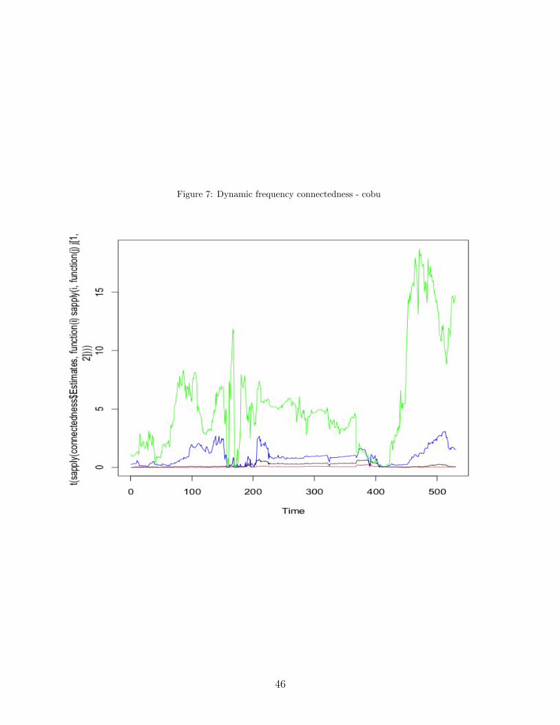
Figure 7: Dynamic frequency connectedness - cobu
46

Figure 8: Dynamic frequency connectedness - Baltic
47

Figure 9: Dynamic frequency connectedness - Russia
Figure 10: Directional Price Spillovers - From Others
48

Figure 11: Directional Price Spillovers - From Others 2
Figure 12: Directional Price Spillovers - to Others
Figure 13: Directional Price Spillovers - to Others 2
49

Figure 14: Directional Volatility Spillovers - From Others
Figure 15: Directional Volatility Spillovers - From Others 2
50

Figure 16: Directional Volatility Spillovers - to Others
Figure 17: Directional Volatility Spillovers - to Others 2
51