pribeiro/Book-Final/SECTION-6-Chapte… · Web viewThe word ‘blind’ emphasizes that the ......

Section 6 - Chapter 5 - Chapter 19 - Harmonic Load Identification Using Independent Component Analysis

Ekrem Gursoy, Dagmar Niebur

519.1 - Introduction

Due to an increase of power electronic equipment and other harmonic sources, the

identification and estimation of harmonic loads is of concern in electric power transmission and

distribution systems. Conventional harmonic state estimation requires a redundant number of

expensive harmonic measurements. In this chapter we explore the use of a statistical signal

processing technique, known as Independent Component Analysis for harmonic source

identification and estimation. If the harmonic currents are statistically independent, ICA is able

to estimate the currents using a limited number of harmonic voltage measurements and

without any knowledge of the system admittances or topology. Results are presented for the

modified IEEE 30 bus system.

Identification and measurement of harmonic sources has become an important issue in

electric power systems, since increased use of power electronic devices and equipments

sensitive to harmonics, has increased the number of adverse harmonic related events.

Harmonic distortion causes financial expenses for customers and electric power

companies. Companies are required to take necessary action to keep the harmonic distortion at

levels defined by standards, i.e. IEEE Standard 519-1992. Marginal pricing of harmonic

injections is addressed in to determine the costs of mitigating harmonic distortion. Harmonic

levels in the power system need to be known to solve these issues. However, in a deregulated

network, it may be difficult to obtain sufficient measurements at substations owned by other

companies.

Harmonic measurements are more sophisticated and costly than ordinary

measurements because they require synchronization for phase measurements, which is

achieved by Global Positioning Systems (GPS). It is not easy and economical to obtain a large

number of harmonic measurements because of instrumentation installation maintenance and

related measurement acquisition issues.

Harmonic state estimation (HSE) techniques have been developed to assess the

harmonic levels and to identify the harmonic sources in electric power systems -. Using

synchronized, partial, asymmetric harmonic measurements, harmonic levels can be estimated

by system-wide HSE techniques . An algorithm to estimate the harmonic state of the network

partially is developed using limited number of measurements . The number and the location of

harmonic measurements for HSE are determined from observability analysis . Either for a fully

observable or a partially observable network, the number of required harmonic measurements

is much larger than the number of sources.

HSE techniques require detailed and accurate knowledge of network parameters and

topology. Approximation of the system model and poor knowledge of network parameters may

lead to large errors in the results. Measurement of harmonic impedances , can be a solution,

which again is impractical and expensive for large networks.

It is therefore very desirable to estimate the harmonic sources without the knowledge

of network topology and parameters, using only a small number of harmonic measurements.

In this chapter we present the estimation of harmonic load profiles of harmonic sources

in the system using a blind source separation algorithm (BSS) which is commonly referred to as

Independent Component Analysis (ICA). The proposed approach is based on the statistical

properties of loads. Both the linear loads and nonlinear loads are modeled as random variables.

519.2 - Independent Component Analysis - ICA Model

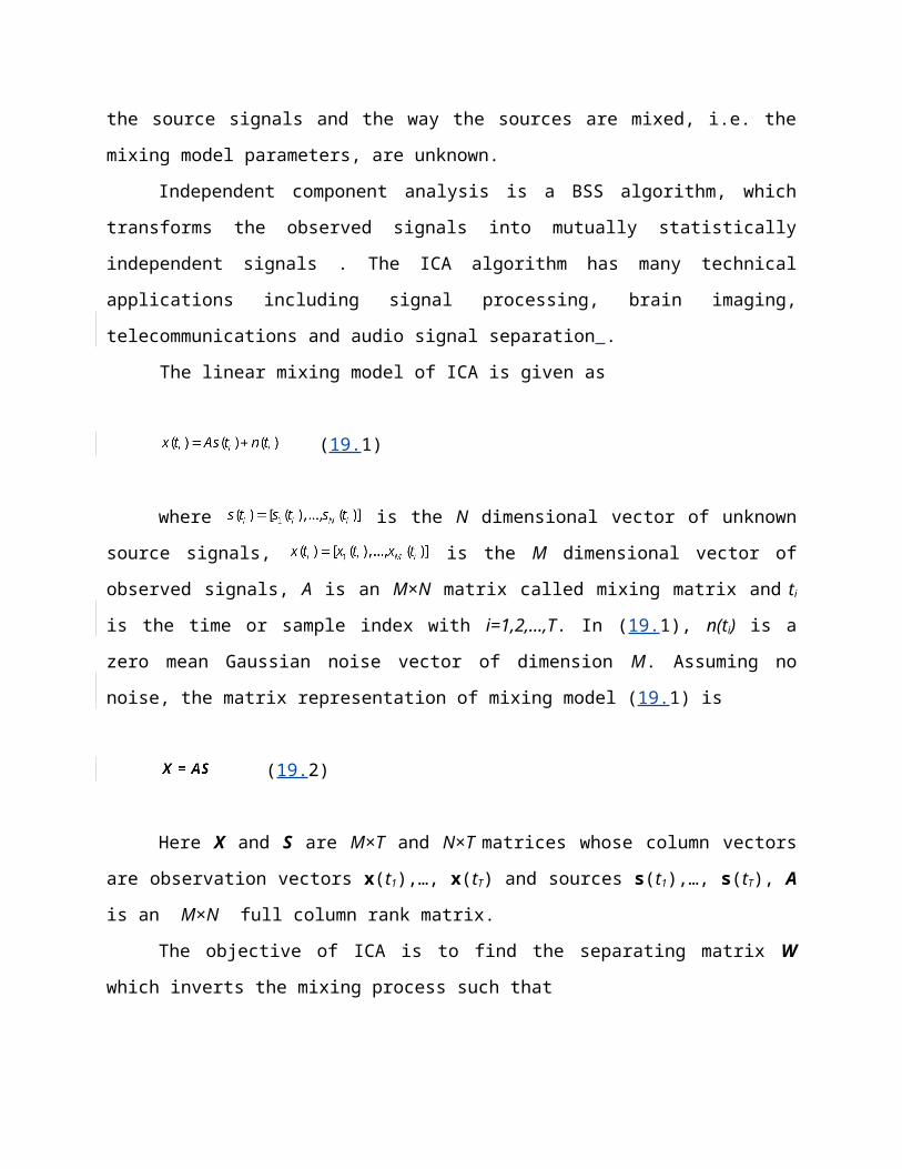
Blind source separation algorithms estimate the source signals from observed mixtures.

The word ‘blind’ emphasizes that the source signals and the way the sources are mixed, i.e. the

mixing model parameters, are unknown.

Independent component analysis is a BSS algorithm, which transforms the observed

signals into mutually statistically independent signals . The ICA algorithm has many technical

applications including signal processing, brain imaging, telecommunications and audio signal

separation .

The linear mixing model of ICA is given as

(19.1)

where is the N dimensional vector of unknown source signals,

is the M dimensional vector of observed signals, A is an M×N matrix called

mixing matrix and ti is the time or sample index with i=1,2,…,T. In (19.1), n(ti) is a zero mean

Gaussian noise vector of dimension M. Assuming no noise, the matrix representation of mixing

model (19.1) is

(19.2)

Here X and S are M×T and N×T matrices whose column vectors are observation vectors

x(t1),…, x(tT) and sources s(t1),…, s(tT), A is an M×N full column rank matrix.

The objective of ICA is to find the separating matrix W which inverts the mixing process

such that

(19.3)

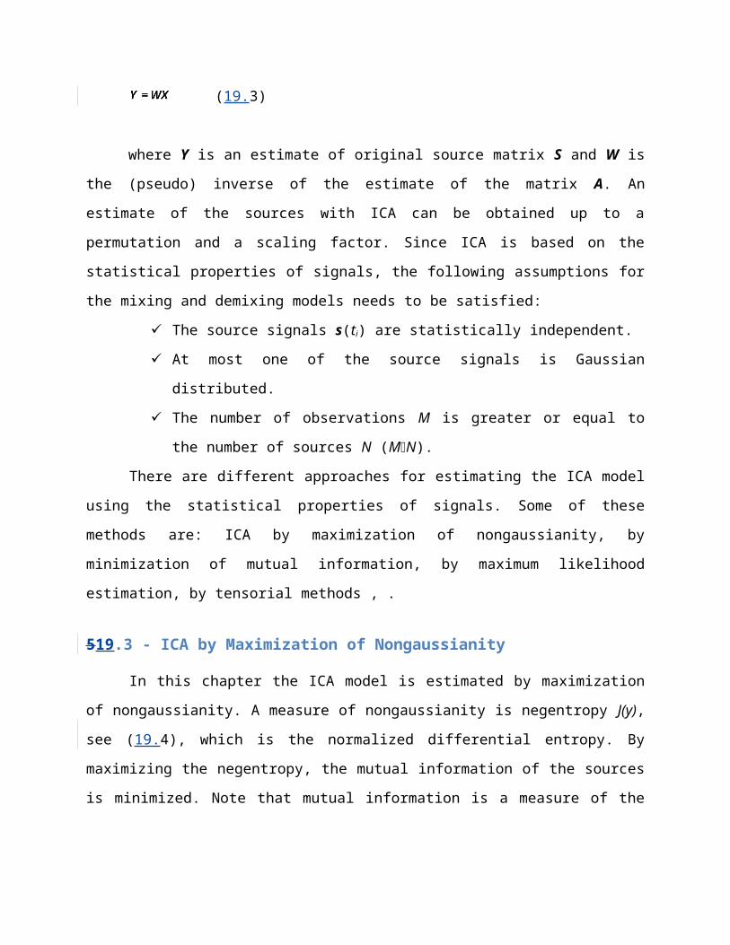
where Y is an estimate of original source matrix S and W is the (pseudo) inverse of the

estimate of the matrix A. An estimate of the sources with ICA can be obtained up to a

permutation and a scaling factor. Since ICA is based on the statistical properties of signals, the

following assumptions for the mixing and demixing models needs to be satisfied:

The source signals s(ti) are statistically independent.

At most one of the source signals is Gaussian distributed.

The number of observations M is greater or equal to the number of sources N

(MN).

There are different approaches for estimating the ICA model using the statistical

properties of signals. Some of these methods are: ICA by maximization of nongaussianity, by

minimization of mutual information, by maximum likelihood estimation, by tensorial methods ,

.

519.3 - ICA by Maximization of Nongaussianity

In this chapter the ICA model is estimated by maximization of nongaussianity. A

measure of nongaussianity is negentropy J(y), see (19.4), which is the normalized differential

entropy. By maximizing the negentropy, the mutual information of the sources is minimized.

Note that mutual information is a measure of the independence of random variables.

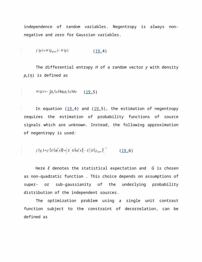
Negentropy is always non-negative and zero for Gaussian variables.

(19.4)

The differential entropy H of a random vector y with density py(η) is defined as

(19.5)

In equation (19.4) and (19.5), the estimation of negentropy requires the estimation of

probability functions of source signals which are unknown. Instead, the following

approximation of negentropy is used:

(19.6)

Here E denotes the statistical expectation and G is chosen as non-quadratic function .

This choice depends on assumptions of super- or sub-gaussianity of the underlying probability

distribution of the independent sources.

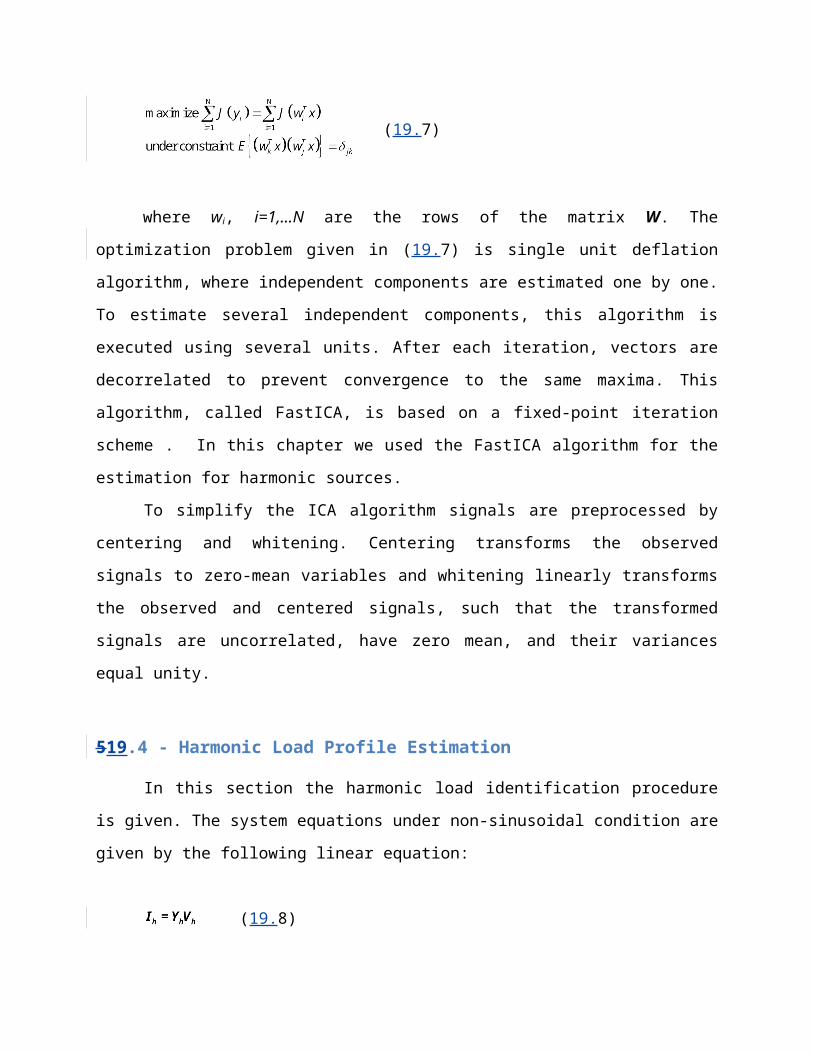
The optimization problem using a single unit contrast function subject to the constraint

of decorrelation, can be defined as

(19.7)

where wi, i=1,…N are the rows of the matrix W. The optimization problem given in (19.7)

is single unit deflation algorithm, where independent components are estimated one by one. To

estimate several independent components, this algorithm is executed using several units. After

each iteration, vectors are decorrelated to prevent convergence to the same maxima. This

algorithm, called FastICA, is based on a fixed-point iteration scheme . In this chapter we used

the FastICA algorithm for the estimation for harmonic sources.

To simplify the ICA algorithm signals are preprocessed by centering and whitening.

Centering transforms the observed signals to zero-mean variables and whitening linearly

transforms the observed and centered signals, such that the transformed signals are

uncorrelated, have zero mean, and their variances equal unity.

519.4 - Harmonic Load Profile Estimation

In this section the harmonic load identification procedure is given. The system equations

under non-sinusoidal condition are given by the following linear equation:

(19.8)

where h is the harmonic order of the frequency, Ih is the bus current injection vector, Vh

is the bus voltage vector and Yh is the system admittance matrix at frequency h. The linear

equation (19.8) is solved for each frequency of interest.

As mentioned in the introduction, it may be difficult to obtain a) accurate system

parameters (Yh), especially for higher harmonics and b) enough harmonic measurements for an

observable system. Using time sequence data of available measurements, i.e. complex

harmonic voltage measurement sequences on a limited number of busses, the ICA approach is

able to estimate the load profiles of harmonic current sources without the knowledge of system

parameters and topology using the statistical properties of time series data only.

The linear measurement model for the harmonic load flow given in (19.8) can be defined

as

(19.9)

Here Vh(ti) M are the known harmonic voltage measurement vectors, Ih(ti) N are

unknown harmonic current source vectors, Zh M×N is the unknown mixing matrix relating

measurements to the sources, n(ti) M is the Gaussian distributed measurement error vector, h

is the harmonic order, ti is the sample index and T is the number of samples. In the presence of

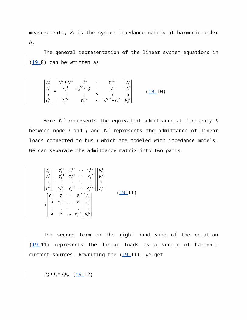
only harmonic voltage measurements, Zh is the system impedance matrix at harmonic order h.

The general representation of the linear system equations in (19.8) can be written as

(19.10)

Here Yhi,j represents the equivalent admittance at frequency h between node i and j and

YhLi represents the admittance of linear loads connected to bus i which are modeled with

impedance models. We can separate the admittance matrix into two parts:

(19.11)

The second term on the right hand side of the equation (19.11) represents the linear

loads as a vector of harmonic current sources. Rewriting the (19.11), we get

(19.12)

Here IhL is the harmonic current source vector corresponding the second term on the

right hand side of (19.11). In the ICA model, the mixing matrix A, which represents the

admittance matrix Yh in the harmonic domain, is required to be time-independent for all time

steps ti, i=1,2,…T. Using this simple manipulation, the load model for linear loads changes from

impedance model to current model and the admittance matrix is kept constant. Using current

models for linear loads increases the number of sources to be estimated in addition to the non-

linear loads. However considering there are no linear loads on harmonic source busses and

combining the linear loads, which have similar load profiles, the number of sources to be

estimated can be reduced.

519.5 - Statistical Properties of Loads

Estimation with ICA requires the statistical independence and non-gaussianity of

sources.

Load profiles of electric loads consist of two parts; a slow varying component and a fast

varying component. Slow varying components represent the variation of loads depending on

the temperature, weather, day of week, time of day etc. Fast varying components can be

modeled as a stochastic process, which represents temporal variation. Generally electrical loads

are not statistically independent because of the slow varying component. This dependency can

be removed by applying a linear filter to the observed data . Fast varying components remain

after filtering the slow varying part of the time series data. Fast fluctuations are assumed to be

statistically independent and non-gaussian distributed. It is shown in for a particular load that

fast fluctuations are statistically independent and that they follow a supergaussian distribution.

Linear filtering of data does not change the mixing matrix A. Therefore, ICA can be applied to

fast varying part of the data and the original sources can be recovered by the estimated

demixing matrix. In studies of probabilistic analysis of harmonic loads, recorded signals are

treated as the sum of deterministic and a random component , ; furthermore harmonic sources

are assumed to be independent similar to the general electric loads.

519.6 - Harmonic Load Estimation

There are some ambiguities in estimation by ICA. Independent components can be

estimated up to a scaling and a permutation factor. This is due to the fact that both the sources

s and the mixing matrix A are unknown. A source can be multiplied by a factor k and the

corresponding column of the mixing matrix can be divided by k, without changing the

probability distribution and the measurement vector. Similarly, permuting two columns of A

and the two corresponding rows of source s will not affect the measurement vector.

This indeterminacy can be eliminated if there is some prior knowledge of sources. In

fact, in electric power systems, it is reasonable to assume that historical load data is available,

which can be used to match the estimated sources to original sources; furthermore it is

assumed that forecasted peak loads are available which can be used to scale the load profiles .

For simplicity, we assume that the number of measurements is equal to the number of

sources. In other words A is a square matrix. If there is a redundancy in measurements, the

dimension of the measurement vector can be reduced using principle component analysis

(PCA).

In this chapter, we assume constant power factor for loads and statistical independence

of loads. Using the FastICA algorithm, we are able to estimate the real and imaginary part of

each harmonic component individually.

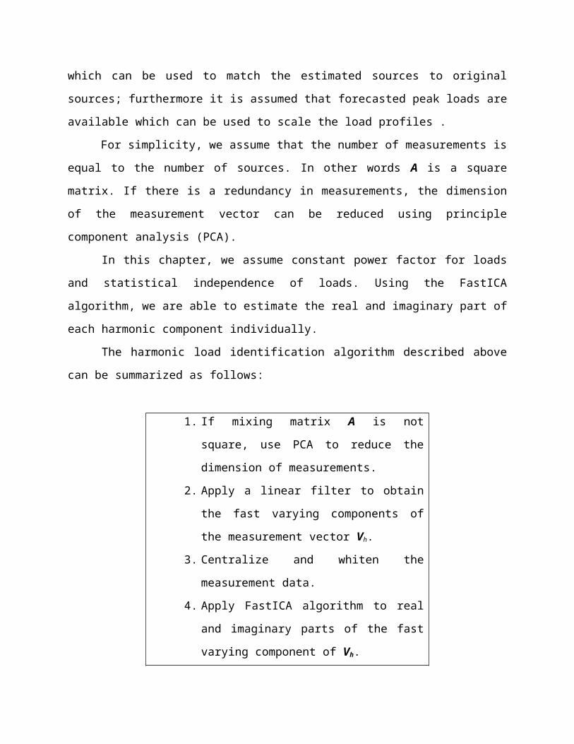
The harmonic load identification algorithm described above can be summarized as

follows:

1. If mixing matrix A is not square, use PCA to

reduce the dimension of measurements.

2. Apply a linear filter to obtain the fast varying

components of the measurement vector Vh.

3. Centralize and whiten the measurement data.

4. Apply FastICA algorithm to real and imaginary

parts of the fast varying component of Vh.

5. Obtain the estimates of real and imaginary parts

of the harmonic current sources at harmonic

frequency h.

6. Perform steps 2 through 5 for each harmonic

component of interest.

7. Reorder and scale the estimated sources using

historical data.

519.7 - Case studies

Case 1

For this chapter typical load profiles were downloaded from the website of Electric

Reliability Council of Texas (ERCOT) . To distinguish fast and slow-varying components of the

normalized and centered load profiles which thus have a zero mean and unity variance, a zero

mean Laplace distributed random variable with 0.02 variance is added to the normalized and

centered load profiles. Here the Laplace distributed random variable represents the fast varying

components, which are statistically independent, and the load profiles represent the slow

varying components mentioned in the previous part. The apparent power of each load is

multiplied by one of these load profiles. Harmonic measurement vectors, i.e. the harmonic bus

voltages, are simulated by harmonic power flow. The public-domain MATPOWER program was

modified to carry out both fundamental and harmonic power flow calculations. First, the

fundamental frequency power flow solution is obtained. Harmonic sources are modeled as

constant power loads in this step. Harmonic current source models are obtained for harmonic

sources using the power flow solution. Next, we calculate the harmonic bus voltages by solving

the linear system equations in (19.8) for each harmonic frequency of interest. In harmonic

analysis, a transmission line, a generator and a transformer are modeled as a π-model, a sub-

transient reactance and a short circuit impedance respectively. The impedance model #2 given

in is used to model linear loads in harmonic domain. The harmonic measurement vector

obtained by harmonic power flow is used in ICA for the estimation of harmonic sources.

The proposed harmonic load identification algorithm is tested on a modified IEEE 30-Bus

test system shown in Fig.19.1. The system is assumed to be balanced. We placed 3 harmonic

producing loads at buses 7, 16 and 30. These buses are geographically and electrically far from

each other, which is usually the case in power systems. These harmonic loads are modeled as

harmonic current injection sources. Harmonic current spectrums given in are used for these

loads and simulations are obtained up to the 17th harmonic. Harmonic source power ratings are

45+j20 MVA, 25 MVar and 25+j16 MVA at bus 7, 16 and 30 respectively. In addition to harmonic

loads, there are 7 linear loads at buses 3, 8, 14, 17, 18, 22, and 25. Four of these linear loads

have a power rating close to harmonic loads power ratings. The remaining buses are no-load

buses. Both the harmonic loads and linear loads have 1-minute varying load shapes, which are

obtained by adding Laplace distributed random variables to slow varying load shapes

normalized to unity and by multiplying them with the power rating of each load. For the

measurements, harmonic voltage measurements are used, since in general these

measurements are easier and more reliable than other harmonic measurements, such as power

measurements. There are 7 harmonic voltage measurement placed at buses 2, 4, 6, 10, 15, 20

and 28. In general it is easier and less expensive to obtain measurements at substations than at

other buses. Therefore six of these measurements are located at substations. None of the

measurements are on the load buses. This reflects the case of a deregulated network where

generation and distribution are unbundled.

The proposed algorithm explained in Part III-B is used to estimate the load shapes of the

harmonic sources. Estimates of the real and imaginary part of the harmonic current sources are

shown in Fig. 19.2-19.4.

Figure 19.1. Modified IEEE 30-Bus system

Figure 19.2 shows the smoothed current profiles of the estimated harmonic current

injection at bus 7. The solid line represents the actual load shapes and the dashed line

represents the estimated ones. The real and imaginary part of the current is estimated

separately by applying the ICA algorithm to real and imaginary part of the observations,

harmonic voltage measurements. Table 19.1 shows the error and the correlation coefficients

between estimated and actual load shapes. The results from Fig. 19.2 and Table 19.1 show that

the proposed algorithm is capable of estimating the load profiles of harmonic injection within a

small error range. Correlation coefficients are close to 1, indicating matching of high accuracy

between estimated and actual profiles.

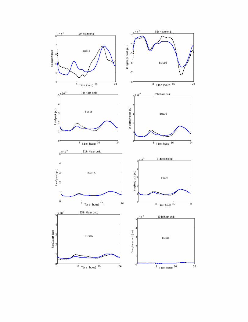
In Fig 19.3 and 19.4, harmonic current injection profiles of the nonlinear loads at bus 16

and 30 are given respectively. The graphs show that there are some slight difference between

estimates and actual shapes. However, estimates are tracking the actual load shapes. Estimates

of the harmonic source at bus 30 are better than the estimates of bus 16. From the figures we

can see that, the high percentage error occurs at small values of current magnitude. Estimates

are more accurate when the magnitude of the current is high. For example, for the imaginary

part of the 5th harmonic, the mean percentage errors are 1.98%, 6.90 % and 2.21% at buses 7,

16 and 30 respectively.

In our simulations, measurement noise is ignored. As investigated in , measurement

noise increases the errors in estimates at lower load levels and additional measurements

increase the performance of the algorithm. In the harmonic domain, the linear loads can be

viewed as distracters adding some non-linearity to the ICA model by changing the mixing matrix

or additional sources as shown in (19.9-19.11). To reduce the effect of the linear loads on the

estimation of harmonic sources, we used more measurements (7 measurements) than the

number of harmonic sources (3 harmonic sources). However, the total number of loads,

including the linear loads, is less than the number of measurements, indicating that there are

some additional effects that contribute to the corruption of the load estimates.

8 16 24-0.04

-0.03

-0.02

-0.01

05th Harmonic

Time (hour)

Rea

l par

t (pu

)

Bus7

8 16 24-0.06

-0.05

-0.04

-0.03

-0.025th Harmonic

Time (hour)

Imag

inar

y pa

rt (

pu)

Bus7

8 16 240.01

0.02

0.03

0.04

0.057th Harmonic

Time (hour)

Rea

l par

t (pu

)

Bus7

8 16 24-0.04

-0.03

-0.02

-0.01

07th Harmonic

Time (hour)

Imag

inar

y pa

rt (

pu)

Bus7

8 16 240

0.01

0.02

0.03

0.0411th Harmonic

Time (hour)

Rea

l par

t (pu

)

Bus7

8 16 24-0.04

-0.03

-0.02

-0.01

011th Harmonic

Time (hour)

Imag

inar

y pa

rt (

pu)

Bus7

8 16 240

0.01

0.02

0.03

0.0413th Harmonic

Time (hour)

Rea

l par

t (pu

) Bus7

8 16 240

0.01

0.02

0.03

0.0413th Harmonic

Time (hour)Im

agin

ary

part

(pu

)

Bus7

8 16 240

0.01

0.02

0.03

0.0417th Harmonic

Time (hour)

Rea

l par

t (pu

)

Bus7

8 16 240

0.01

0.02

0.03

0.0417th Harmonic

Time (hour)

Imag

inar

y pa

rt (

pu)

Bus7

Figure 19.2. Harmonic components of current injection at Bus 7

Table 19.1. ERRORS BETWEEN ESTIMATED AND ACTUAL SMOOTHED HARMONIC CURRENT PROFILES AT BUS 7

Harmonic

Order

Correlation

Coefficient

Maximum

Percentage

Error (%)

Mean Percentage Error (%)

5Real 0.9988 2.73 0.73

Imag 0.9932 5.30 1.98

7Real 0.9964 4.71 1.74

Imag 0.9975 3.81 1.39

11 Real 0.9933 5.43 2.31

BUS

7Imag 0.9974 3.20 1.47

13Real 0.9989 5.51 1.54

Imag 0.9967 3.77 1.15

17Real 0.9992 2.71 0.67

Imag 0.9713 9.38 2.29

8 16 243

4

5

6

7

8 x 10-3 5th Harmonic

Time (hour)

Rea

l par

t (pu

) Bus16

8 16 24-8

-7

-6

-5

-4

-3 x 10-3 5th Harmonic

Time (hour)

Imag

inar

y pa

rt (

pu)

Bus16

8 16 240

1

2

3

4


Time (hour)

Rea

l par

t (pu

)

Bus16

8 16 241

2

3

4

5


Time (hour)

Imag

inar

y pa

rt (

pu)

Bus16

8 16 240

1

2

3

4


Time (hour)

Rea

l par

t (pu

)

Bus16

8 16 240

1

2

3

4


Time (hour)

Imag

inar

y pa

rt (

pu)

Bus16

8 16 240

1

2

3

4


Time (hour)

Rea

l par

t (pu

)Bus16

8 16 240

1

2

3

4


Time (hour)

Imag

inar

y pa

rt (

pu)

Bus16

8 16 24-5

-4

-3

-2

-1


Time (hour)

Rea

l par

t (pu

)

Bus16

8 16 240

1

2

3

4


Time (hour)

Imag

inar

y pa

rt (

pu)

Bus16


Table 19.2. errors between estimated and actual smoothed harmonic current profiles at bus 16

Harmonic

Order

Correlation

Coefficient

Maximum

Percentage

Error (%)


BUS

16

5Real 0.6825 24.85 14.58

Imag 0.9309 21.91 6.90

7Real 0.9122 21.44 7.70

Imag 0.9461 12.30 4.38

11Real 0.9857 9.03 2.15

Imag 0.9121 16.15 6.12

13Real 0.6780 36.34 14.96

Imag 0.5429 42.42 11.48

17Real 0.7476 25.84 9.28

Imag 0.6849 35.78 11.92

8 16 24-10

-8

-6

-4

-2

05th Harmonic

Time (hour)

Rea

l par

t (pu

) Bus30

x 10 -3

8 16 24-32

-30

-28

-26

-24

-225th Harmonic

Time (hour)

Imag

inar

y pa

rt (

pu)

Bus30

x 10 -3

8 16 24-18

-16

-14

-12

-10

7th Harmonic

Time (hour)

Rea

l par

t (pu

)

Bus30

x 10 -3

8 16 24-20

-18

-16

-14

-12

-107th Harmonic

Time (hour)

Imag

inar

y pa

rt (

pu)

Bus30

x 10 -3

8 16 24-12

-10

-8

-6

-4

-2 x 10-3 11th Harmonic

Time (hour)

Rea

l par

t (pu

) Bus30

8 16 240

2

4

6

8

1011th Harmonic

Time (hour)

Imag

inar

y pa

rt (

pu)

Bus30

x 10 -3

8 16 24-10

-8

-6

-4

-2

013th Harmonic

Time (hour)

Rea

l par

t (pu

)

Bus30

x 10 -3

8 16 240

2

4

6

8

1013th Harmonic

Time (hour)

Imag

inar

y pa

rt (

pu)

Bus30

x 10 -3

8 16 240

2

4

6

8

1017th Harmonic

Time (hour)

Rea

l par

t (pu

)

Bus30

x 10 -3

8 16 240

2

4

6

8

1017th Harmonic

Time (hour)

Imag

inar

y pa

rt (

pu)

Bus30

x 10 -3


Table 19.3. errors between estimated and actual smoothed harmonic current profiles at bus 30

Harmonic

Order

Correlation

Coefficient

Maximum

Percentage

Error (%)


BUS

30

5Real 0.6150 27.13 11.59

Imag 0.9640 6.39 2.21

7Real 0.9592 7.21 2.15

Imag 0.9525 7.55 2.66

11Real 0.9485 7.95 3.20

Imag 0.8817 19.39 8.47

13Real 0.9669 5.43 1.81

Imag 0.8787 15.07 6.02

17Real 0.8940 12.97 5.96

Imag 0.9398 10.18 3.14

Case 2In this case, the estimation process is based on fewer measurements in order to test the

effectiveness of the proposed algorithm for estimating the largest harmonic source in the

network. Using the same test system as in Fig. 19.1, two harmonic voltage measurements are

taken from bus 2 and 4 instead of seven measurements as in Case 1.

Estimation results for the harmonic source at bus 7 are given in Table 19.4. Using the

ICA algorithm, this harmonic load is estimated with a small error. Second output of the ICA

estimation can not be matched with other two harmonic sources at Bus 16 and 30, because the

correlation coefficients are small, i.e. 0.3516 and 0.4587.

Table 19.4. errors between estimated and actual smoothed harmonic current profiles at bus 7 with 2 harmonic measurements

Harmonic

Order

Correlation

Coefficient

Maximum

Percentage

Error (%)


BUS

7

5Real 0.9982 3.29 1.00

Imag 0.9916 6.31 2.26

7Real 0.9949 6.20 2.02

Imag 0.9989 2.62 0.79

11Real 0.9989 2.09 0.90

Imag 0.9993 2.17 0.54

13Real 0.9977 5.21 1.06

Imag 0.9983 2.25 1.12

17Real 0.9417 16.68 6.48

Imag 0.9593 8.95 2.38

From the results given in Case 1 and 2, we can see that, the harmonic source with

harmonic current rating higher than the other system loads, can be estimated with a very good

range of error.

As future work, the impact of the location and number of measurements as well as the

number time steps per measurement on the accuracy of the estimation needs further

investigation.

519.8 - Conclusion

Independent Component Analysis is used to estimate the load profiles of harmonic

sources without prior knowledge of network topology and parameters. This method is based on

the statistical properties of loads. Statistical independence of loads is assured by separating the

fast and slow varying components in load profiles using a linear filter and by using only the fast-

varying component for the independent component analysis. The application of the proposed

algorithm to the modified IEEE 30-Bus test system shows that current profiles of harmonic

sources can be estimated using only a small number of harmonic voltage measurements.

The proposed method is quite promising for the application in a deregulated network

since the number of measurements is small and the measurements can be taken far from the

sources. Also this algorithm can be extended to find the minimum set of measurements to

reduce the measurements cost and increase estimation accuracy for the harmonic meter

placement problem.

Acknowledgment

The authors would like to acknowledge Huaiwei Liao’s help in the early stages of this work.

519.9 References

pribeiro/Book-Final/SECTION-6-Chapte… · Web viewThe word ‘blind’ emphasizes that the ......

Documents

Transcript of pribeiro/Book-Final/SECTION-6-Chapte… · Web viewThe word ‘blind’ emphasizes that the ......