Previous Lecture: NGS Alignment

NGS Alignment

Spring CHIBI Courses• BMI Foundations I: Bioinformatics (BMSC-GA 4456)

• Constantin Aliferis– Study classic Bioinformatics/Genomics papers and reproduce data analysis, for advanced

informatics students

• Integrative Genomic Data Analysis (BMSC-GA 4453)• Jinhua Wang

– build competence in quantitative methods for the analysis of high-throughput genomic data• Microbiomics Informatics (BMSC-GA 4440)

• Alexander Alekseyenko– analysis of microbial community data generated by sequencing technologies: preprocess raw

sequencing data into abundance tables, associate abundance with clinical phenotype and outcomes.

• Next Generation Sequencing (BMSC-GA 4452)• Stuart Brown

– An overview of Next-Generation sequencing informatics methods for data pre-processing, alignment, variant detection, structural variation, ChIP-seq, RNA-seq, and metagenomics.

• Proteomics Informatics (BMSC-GA 4437)• David Fenyo

– A practical introduction of proteomics and mass spectrometry workflows, experimental design, and data analysis

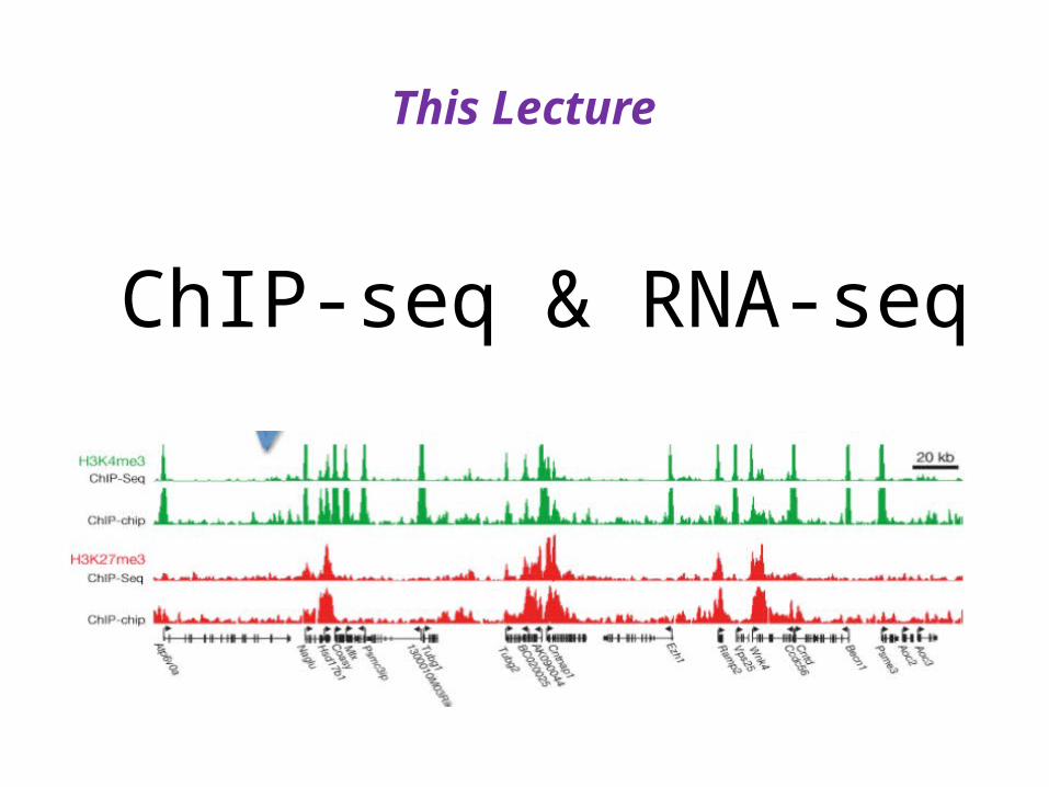
ChIP-seq & RNA-seq

This Lecture

Learning Objectives

• ChIP-seq experimental methods• Transcription factors and epigenetics

• Alignment and data processing• Finding peaks: MACS algorithm• Annotation

• RNA-seq experimental methods• Alignment challenges (splice sites)

• TopHat• Counting reads per gene

• Normalization• HTSeq-count and Cufflinks

• Statistics of differential expression for RNA-seq

ChIP-seq

• Combine sequencing with Chromatin‐Immunoprecipitaion

• Select (and identify) fragments of DNA that interact with specific proteins such as: – Transcription factors – Modified histones – Methylation– RNA Polymerase (survey actively transcribe portions of the

genome) – DNA polymerase (investigate DNA replication)– DNA repair enzmes

ChIP-chip

• [Pre-sequencing technology] • Do chromatin IP with YFA (Your Favorite Antibody)• Take IP-purified DNA fragments, label & hybridize to a

microarray containing (putative) promoter (or TF binding) sequences from lots of genes

• Estimate binding, relate to DNA binding of protein targeted by antibody– limited to well annotated genomes – need to build special microarrays – suffers from hybridization bias– assumes all TF binding sites are known and correctly located on

genome

Release DNA

Immunoprecipitate

High-throughput sequencing

Map sequence tags to genome

ChIP-seq

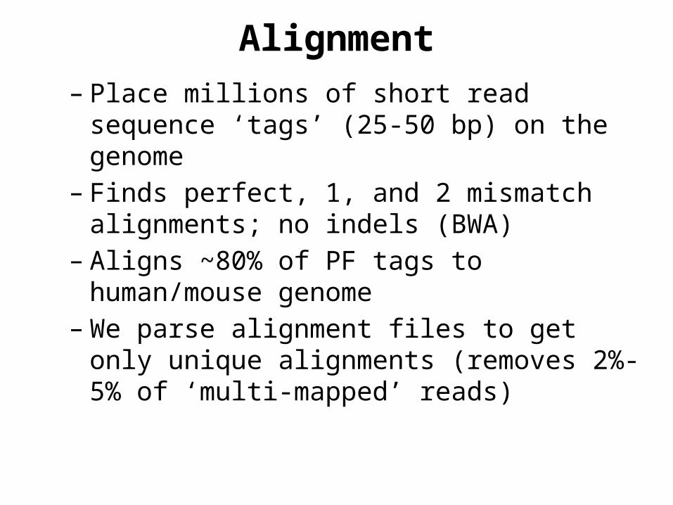
– Place millions of short read sequence ‘tags’ (25-50 bp) on the genome

– Finds perfect, 1, and 2 mismatch alignments; no indels (BWA)

– Aligns ~80% of PF tags to human/mouse genome

– We parse alignment files to get only unique alignments (removes 2%-5% of ‘multi-mapped’ reads)

Alignment

ChIP-seq for TF

Jothi, et al. Genome-wide identification of in vivo protein–DNA binding sites from ChIP-Seq data. NAR (2008), 36: 5221-31

(SISSRS software)

Saturation• How many sequence reads are needed to

find all of the binding targets in the genome?• Look for plateau

20 30 40 50 60 70 80 900

20

40

60

80

100

120

Pol2 data: 11M reads vs. 12M control reads, peaks found with MACS, data sub-sampled.

100% = 15,291 peaks

Rozowsky, et al. Nature Biotech. Vol 27-1, Jan 2009.

ChIP-seq Challenges

• We want to find the peaks (enriched regions = protein binding sites on genome)

• Goals include: accuracy (location of peak on genome), sensitivity, & reproducibility

• Challenges: non-random background, PCR artifacts, difficult to estimate false negatives

• Very difficult to compare samples to find changes in TF binding (many borderline peaks)

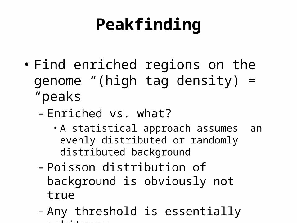
Peakfinding

• Find enriched regions on the genome (high tag density) = “peaks”– Enriched vs. what?

• A statistical approach assumes an evenly distributed or randomly distributed background

– Poisson distribution of background is obviously not true

– Any threshold is essentially arbitrary

Compare to Background• Goal is to make ‘fold change’

measurements• What is the appropriate background?

– Input DNA (no IP)– IP with non-specific antibody (IgG)

[We mostly use input DNA]

• Must first identify “peak region” in sample, then compare tag counts vs BG

MACS• Zhang et al. Model-based Analysis of ChIP-Seq (MACS).

Genome Biol (2008) vol. 9 (9) pp. R137• Open source Unix software (Python !)

– MACS improves the spatial resolution of binding sites through combining the information of sequencing tag position and orientation by using empirical models for the length of the sequenced ChIP fragments

• (slides + and – strand reads toward center of fragment)

– MACS uses a dynamic Poisson distribution (local background count in the control) to effectively capture local biases in the genome sequence, allowing for more sensitive and robust prediction

– Uses control to calculate “random” peaks, sets FDR rate.

Feng J, Liu T, Zhang Y. Using MACS to identify peaks from ChIP-Seq data. Curr Protoc Bioinformatics. 2011 Jun;Chapter 2:Unit 2.14.

BED format• BED format defines a genomic interval as positions on a reference

genome.• An interval can be a anything with a location: gene, exon, binding site,

region of low complexity, etc. • MACS outputs ChIP-seq peaks in BED format• BED files can also specify color, width, some other formatting.

chr1 213941196 213942363 chr1 213942363 213943530 chr1 213943530 213944697 chr2 158364697 158365864 chr2 158365864 158367031 chr3 127477031 127478198 chr3 127478198 127479365 chr3 127479365 127480532

chromosome start end

track name="ItemRGBDemo" description="Item RGB demonstration" itemRgb="On" chr7 127471196 127472363 Pos1 0 + 127471196 127472363 255,0,0 chr7 127472363 127473530 Pos2 0 + 127472363 127473530 255,0,0 chr7 127473530 127474697 Pos3 0 + 127473530 127474697 255,0,0 chr7 127474697 127475864 Pos4 0 + 127474697 127475864 255,0,0 chr7 127475864 127477031 Neg1 0 - 127475864 127477031 0,0,255 chr7 127477031 127478198 Neg2 0 - 127477031 127478198 0,0,255 chr7 127478198 127479365 Neg3 0 - 127478198 127479365 0,0,255 chr7 127479365 127480532 Pos5 0 + 127479365 127480532 255,0,0

Remove Duplicates

• In some ChIP-seq samples, PCR amplification of IP-enriched DNA creates artifacts (highly duplicated fragments)

• Huge differences depending on target of antibody and amount of IP DNA collected.

• “Complexity” of the library

PCR ‘stacks’

• Always in F-R pairs, ~200 bp apart

% of Duplicates varies

Different IP Targets

• Huge difference between Transcription Factors and Histone modification as targets of IP

TF• sequence-specific

binding motifs• few thousand sites• binding region ~50bp• oriented tags• yes/no binding• promoters or

enhancers

Histone Mods• not sequence-specific• tens to hundreds of

thousands of sites• large binding region

(~2kb)• tags not oriented• signal may be scaled• associated w/ almost

all transcribed genes

Mikkelsen, Lander, et al. Genome-wide maps of chromatin state in pluripotent and lineage-committed cells. Nature (2007) 448: 553-562.

H3K4me3

Normalization

• How to compare lanes with different numbers of reads?

• Will bias fold-change calculations• Simple method – set all counts in ‘peak’

regions as per million reads– This does not work well for >2x differences in

read counts.

Evaluation

• Peaks near promoters of known genes (TSS)

• Generally a high %• As parameters become less stringent, more

peaks are found, % near TSS declines

• Estimate false positive rate• Pure statistical (Poisson or Monte Carlo)• Compare 2 bg sampels (QuEST)• Reverse sample & bg (MACS)• Can’t estimate false negative rate – don’t know

‘true’ number of binding sites

Evaluation• Overlap with ChIP-chip data

• What is an overlap?• What % overlap is good?

• Reproducibility• Need to define (we use overlap of 1 bp)• Very important for biological conclusions• Essential for comparisons of diff. conditions• Must have replicate samples!!• Trade off: reproducibility vs. sensitivity

• Synthetic data• Allows calculation of sensitivity & specificity• How similar to real data? (All synth has bias)

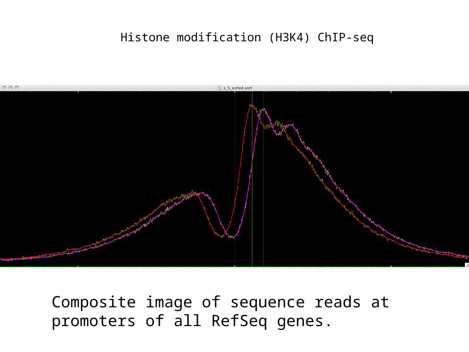
Histone modification (H3K4) ChIP-seq

Composite image of sequence reads at promoters of all RefSeq genes.

The Use of Next Generation Sequencing to Study Transcriptomes:

RNA-seq

RNA-seq Measures the Transcriptome

• Takes advantage of the rapidly dropping cost of Next-Generation DNA sequencing

• Measures gene expression in true genome-wide fashion (all the RNA)

• Also enables detection of mutations (SNPs), alternative splicing, allele specific expression, and fusion genes

• More accurate and better dynamic range than Microarray

• Can be used to detect miRNA, ncRNA, and other non-coding RNA

RNA-seq Measures the Transcriptome

• Takes advantage of the rapidly dropping cost of Next-Generation DNA sequencing

• Measures gene expression in true genome-wide fashion (all the RNA)

• Also enables detection of mutations (SNPs), alternative splicing, allele specific expression, and fusion genes

• More accurate and better dynamic range than Microarray

• Can be used to detect miRNA, ncRNA, and other non-coding RNA

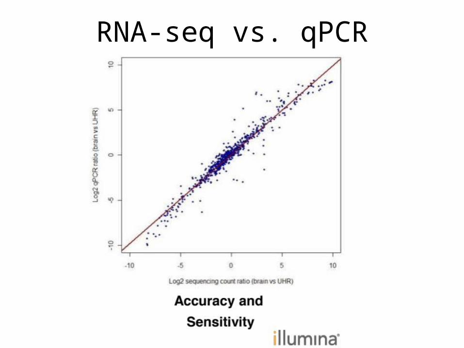
RNA-seq vs. qPCR

Depth of Coverage

• With the Illumina HiSeq producing >200 million reads per sample, what depth of coverage is needed for RNA-seq?

• Can we multiplex several samples per lane and save $$ on sequencing?

• For expression profiling (and detection of differentially expressed genes), probably yes, 2-4 samples per lane is practical

Toung, et al. Genome Res. 2011 June; 21(6): 991–998..

100 million reads, 81% of genes FPKM ≥ 0.05Each additional 100 million reads detects ~3% more genes

Illumina mRNA Sequencing

Poly-A selection

Random primer PCR

Fragment & size-select

Sample prep can create 3’ or 5’ bias

5’ bias(strand oriented protocol)

no bias (low coverage at ends

of transcript)

3’ bias (poly-A selection)

Detect Small RNAs – depends on sample prep method

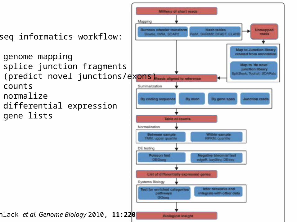
Oshlack et al. Genome Biology 2010, 11:220

RNA-seq informatics workflow:

• genome mapping• splice junction fragments• (predict novel junctions/exons)• counts• normalize• differential expression• gene lists

RNA-seq Alignment Challenges

• Using RNA-seq for gene expression requires counting sequence reads per gene

• Must map reads to genes – but this is a more difficult problem than mapping reads to a reference genome

• Introns create big gaps in alignment• Small reads mean many short overlaps at one end or the

other of intron gaps• What to do with reads that map to introns or outside

exon boundaries?• What about overlapping genes?

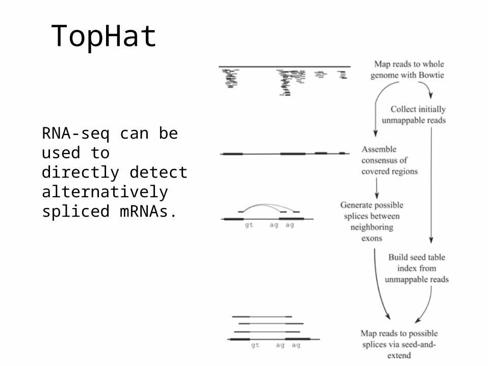
TopHat

RNA-seq can be used to directly detect alternatively spliced mRNAs.

Map reads to exons & junctions

The seed and extend alignment used to match reads to possible splice sites.

Trapnell C et al. Bioinformatics 2009;25:1105-1111

TopHat

Real data generally support existing annotation

Data from Costa lab

RNA-seq informatics• Filter out rRNA, tRNA, mitoRNA• Align to genome• Find splice junction fragments (join exon

boundaries)• Differential expression• Alternatively spliced transcripts• Novel genes/exons• Sequence variants (SNPs, indels,

translocations)• Allele-specific expression

Count Reads per gene

• Need a reference genome with exon information

• How to count partial alignments, novel splices etc?

• Simple or complex model?– Simple: HTSeq-count– Complex: Cufflinks

• Normalization methods affect the count very dramatically

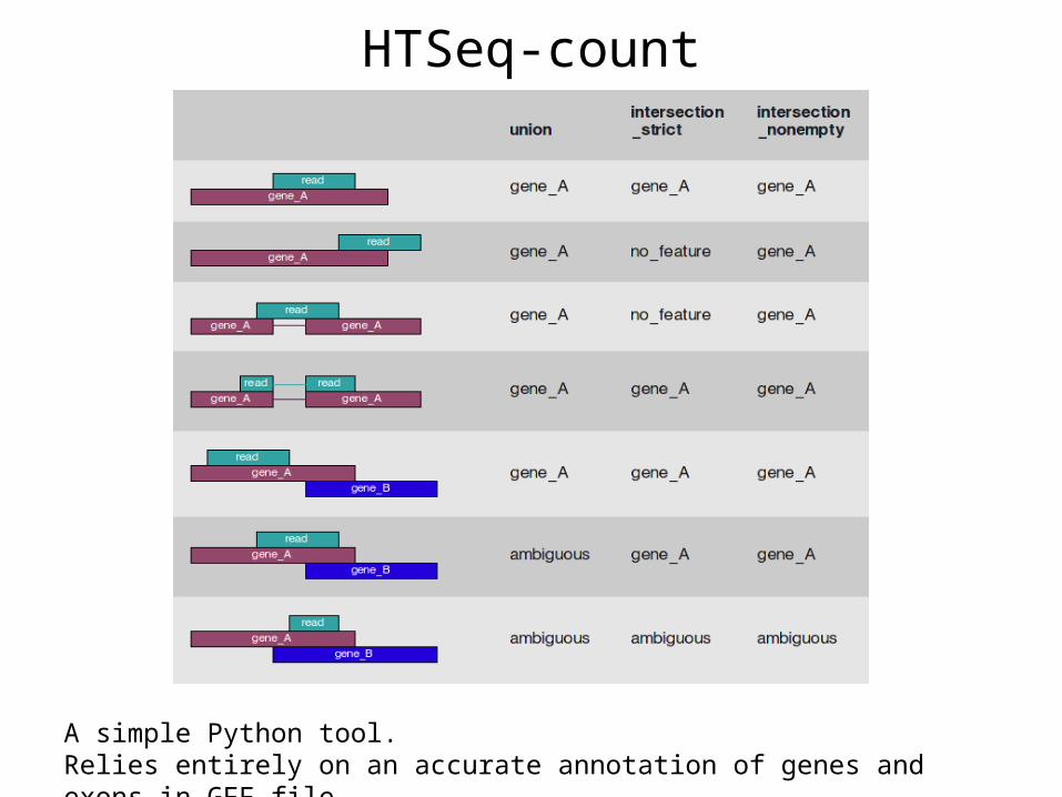
HTSeq-count

A simple Python tool. Relies entirely on an accurate annotation of genes and exons in GFF file.

Cufflinks Isoform Models

ADM

Differential Expression

Data from Costa Lab

Normalization• Differential Expression (DE) requires comparison of 2 or

more RNA-seq samples.• Number of reads (coverage) will not be exactly the

same for each sample• Problem: Need to scale RNA counts per gene to total

sample coverage• Solution – divide counts per million reads

• Problem: Longer genes have more reads, gives better chance to detect DE

• Solution – divide counts by gene length

• Result = RPKM (Reads Per KB per Million)

Better Normalization• RPKM assumes:

• Total amount of RNA per cell is constant• Most genes do not change expression

• RPKM is invalid if there are a few very highly expressed genes that have dramatic change in expression (dominate the pool of reads)

• Better to use “Upper Quartile” (75th percentile) or “Quantile” normalization

• Different normalization methods give different results (different DE genes & different p-value rankings)

Statistics of DE• mRNA levels are variable in cells/tissues/organisms

over time/treatment/tissue etc. • Like microarrays, need replicates to separate

biological variability from experimental variability• If there is high experimental variability, then

variance within replicates will be high, statistical significance for DE will be difficult to find.

• Best methods to discover DE are coupled with sophisticated approaches to normalization

• Best to ignore very low expressing genes: RPKM<1

Popular DE Statistical methods• Cufflinks-Cuffdiff

• part of TopHat software suite – easy to use• Uses FPKM normalization• complex model for counting reads among splice variants

– can be set to ignore novel variants

• Estimates variance in log fold change for each gene using permutations• finds the most DE genes, high false positive rate

• edgeR • requires raw count data, does its own normalization• Estimates standard deviation (dispersion) with a weighted combination of individual gene

(gene-wise) and global measures• Statistical model is Negative Binomial distribution (has a dispersion parameter)• Fisher’s Exact test (for 2-sample), or generalized linear model (complex design)• acceptable tradeoff of sensitivity and specificity

• Many others: DESeq, SAMseq, baySeq. • Many rather inconclusive benchmarking studies

DE genes by different methods

Differentially expressed genes

Data from Meruelo Lab70% of DE genes validated by qPCR

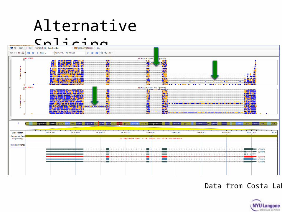
Alternative Splicing

Data from Costa Lab

Good SNP

data from Zavadil lab

Novel Genomes• RNA-seq can be used to annotate genomes –

gene discovery, exon mapping.

data from Desplan lab

Summary

• ChIP-seq experimental methods• Transcription factors and epigenetics

• Alignment and data processing• Finding peaks: MACS algorithm• Annotation

• RNA-seq experimental methods• Alignment challenges (splice sites)

• TopHat• Counting reads per gene

• Normalization• HTSeq-count and Cufflinks

• Statistics of differential expression for RNA-seq

Next Lecture: Signal Processing