Preview Control for Wind Turbines

A DISSERTATION

SUBMITTED TO THE FACULTY OF THE GRADUATE SCHOOL

OF THE UNIVERSITY OF MINNESOTA

BY

Ahmet Arda Ozdemir

IN PARTIAL FULFILLMENT OF THE REQUIREMENTS

FOR THE DEGREE OF

Doctor of Philosophy

Professor Gary J. Balas

Professor Peter J. Seiler

August, 2013

c⃝ Ahmet Arda Ozdemir 2013

Section 5.4: c⃝ 2013 IEEE. Reprinted, with permission, from

Ahmet Arda Ozdemir, Peter Seiler, Gary J. Balas,

Design Tradeoffs of Wind Turbine Preview Control,

IEEE Transactions on Control Systems Technology, July, 2013

ALL RIGHTS RESERVED

Acknowledgements

I would like to express my endless gratitude for my advisers Gary Balas and Pete Seiler.

They have been exceptional guides throughout my graduate studies. They taught me

how to think. What I have learned from them is above and beyond what is contained

in this thesis. I have been very lucky to have them as my advisers. They will remain

as my role models as I progress beyond my graduate studies. I will strive to live up to

their high standards.

I would like to thank my thesis committee members Mihailo R. Jovanovic and Demoz

Gebre-Egziabher. I learned a great deal from their excellent classes. Their feedback on

my research and my thesis was very valuable.

The current and past members of the Lab 309, or formerly Lab 15 as I prefer to

call it, have enriched my graduate school experience with their sincere friendship and

knowledge. I would like to acknowledge Paul, Andrei, Claudia, Abhijit, Arnar, David,

Will, Shu and Bin. We spent countless hours talking about many topics ranging from

control theory to random bits of life during our lunch breaks, happy hours and the ‘I

am stuck on my research’ breaks we had throughout the day. It was time well spent: I

owe my sanity to those moments.

No less important are my friends Kamran, Pietro, Kyung-Hoon, Eyoab and Davide.

I have shared countless memories with them that made my time in Minneapolis a special

chapter in my life. I would also like to thank Miao for her support during the initial

years of my studies.

I am very grateful for the patience and understanding of Briahna. This thesis took

away many hours of my time from her. I especially thank her for bearing with the

boring me while I was busy writing all the time. I deeply appreciate her support.

Last but not least, I would like to thank my parents for their unwavering love.

i

Dedicated to my parents: Zumral and Nutullah Ozdemir

ii

Abstract

The success of wind power as a renewable energy source depends on its cost of energy.

Wind turbine control has attracted much attention in the controls community due to its

potential impact on the cost of wind power. However, novel methods in the literature

have not transitioned well to industry. This is because the potential cost benefits of

these methods are not well understood. There is a need for basic research to address

this issue.

This thesis is one step toward transitioning of advanced control methods in literature

to the industry. Particularly, we aim to understand the limits of performance. The

potential performance improvements of the advanced methods should be large enough

to justify their cost and complexity. We investigate the optimal trade-offs between

multiple turbine performance goals. We also explore the use of a novel wind preview

sensor in closed-loop control laws. The impact of this novel sensor on the optimal

turbine performance is investigated.

The specific contributions of this thesis can be grouped in three categories. First, we

present a preliminary, nonlinear optimization based controller design and analysis frame-

work. This framework can simplify the design of the advanced multivariable controllers

for nonlinear systems. It can also be used to investigate the optimal design trade-offs

between nonlinear performance constraints and objectives. Second, engineering insight

is provided into turbine design trade-offs. Third, we provide mathematical tools that

quantify the limits of turbine performance in presence of preview wind measurements.

Optimization tools that can analyze the trade-off between preview time and operating

condition dependent turbine performance objectives are presented. In low wind speeds,

our results show that simultaneous power capture improvements and structural load

reductions can be obtained. In high wind speeds, a short amount of preview wind in-

formation can be used to overcome the fundamental performance limitations imposed

by actuator rate constraints. We provide analytical formulas that quantify these pre-

view time requirements and performance limitations. A convex optimization framework

is also presented for the analysis of extreme operating conditions that are defined by

deterministic wind disturbance trajectories.

iii

Contents

Acknowledgements i

Abstract iii

List of Tables vii

List of Figures viii

1 Introduction 1

1.1 Thesis Overview . . . . . . . . . . . . . . . . . . . . . . . . . . . . . . . 3

1.2 Thesis Contributions . . . . . . . . . . . . . . . . . . . . . . . . . . . . . 5

2 Background 7

2.1 Introduction . . . . . . . . . . . . . . . . . . . . . . . . . . . . . . . . . . 7

2.2 Types of Turbine Designs . . . . . . . . . . . . . . . . . . . . . . . . . . 8

2.3 Basics of Horizontal-Axis Turbine Operation . . . . . . . . . . . . . . . 10

2.4 Current Approaches and Challenges . . . . . . . . . . . . . . . . . . . . 12

3 Wind Turbine Modeling 16

3.1 Introduction . . . . . . . . . . . . . . . . . . . . . . . . . . . . . . . . . . 16

3.2 Overview of Turbine Modeling . . . . . . . . . . . . . . . . . . . . . . . 17

3.3 Lower Fidelity Models . . . . . . . . . . . . . . . . . . . . . . . . . . . . 21

3.4 Medium Fidelity Models . . . . . . . . . . . . . . . . . . . . . . . . . . . 22

3.4.1 Turbine Dynamics . . . . . . . . . . . . . . . . . . . . . . . . . . 22

3.4.2 Actuator Dynamics . . . . . . . . . . . . . . . . . . . . . . . . . . 25

iv

3.4.3 LIDAR Sensor Dynamics . . . . . . . . . . . . . . . . . . . . . . 26

3.5 Linear System Approximations . . . . . . . . . . . . . . . . . . . . . . . 27

3.5.1 Linear Time Varying via Linearization . . . . . . . . . . . . . . . 28

3.5.2 LTI Approximation and Multiblade Coordinate Transformation . 30

4 Multivariable Control Design 34

4.1 Introduction . . . . . . . . . . . . . . . . . . . . . . . . . . . . . . . . . . 34

4.2 Multivariable Control Design Framework . . . . . . . . . . . . . . . . . . 36

4.2.1 Problem Formulation . . . . . . . . . . . . . . . . . . . . . . . . 36

4.2.2 Design Process . . . . . . . . . . . . . . . . . . . . . . . . . . . . 39

4.2.3 Auto-Tuning Framework . . . . . . . . . . . . . . . . . . . . . . . 43

4.3 Example Problem: Turbine Region 3 Controllers . . . . . . . . . . . . . 45

4.3.1 Linear Model and Input-Measurement Transformations . . . . . 47

4.3.2 H∞ Design Interconnection and the Initial Design . . . . . . . . 49

4.3.3 Cost and Constraint Functions . . . . . . . . . . . . . . . . . . . 52

4.3.4 Gradient-based Optimization . . . . . . . . . . . . . . . . . . . . 54

4.4 Example Problem Results . . . . . . . . . . . . . . . . . . . . . . . . . . 54

4.5 Conclusions and Recommendations . . . . . . . . . . . . . . . . . . . . . 59

5 Preview Control 61

5.1 Introduction . . . . . . . . . . . . . . . . . . . . . . . . . . . . . . . . . . 61

5.2 Related Work . . . . . . . . . . . . . . . . . . . . . . . . . . . . . . . . . 63

5.3 Region 2 Preview Control . . . . . . . . . . . . . . . . . . . . . . . . . . 64

5.3.1 Problem Formulation . . . . . . . . . . . . . . . . . . . . . . . . 65

5.3.2 Power Capture versus Drivetrain Loads Trade-off . . . . . . . . . 71

5.4 Region 3 Preview Control . . . . . . . . . . . . . . . . . . . . . . . . . . 76

5.4.1 Analytical Results for One-State Turbine Model . . . . . . . . . 77

5.4.2 Validation with H∞ Preview Controllers . . . . . . . . . . . . . . 87

5.5 Preview Control for Extreme Events . . . . . . . . . . . . . . . . . . . . 99

5.5.1 Problem Formulation . . . . . . . . . . . . . . . . . . . . . . . . 101

5.5.2 Analysis of a 50-Year Gust . . . . . . . . . . . . . . . . . . . . . 104

5.5.3 Generalizations . . . . . . . . . . . . . . . . . . . . . . . . . . . . 108

5.6 Conclusions . . . . . . . . . . . . . . . . . . . . . . . . . . . . . . . . . . 109

v

6 Conclusions and Recommendations 111

References 116

vi

List of Tables

4.1 Optimization Results . . . . . . . . . . . . . . . . . . . . . . . . . . . . . 55

5.1 Atmospheric parameters used in TurbSim for generating turbulent wind

data . . . . . . . . . . . . . . . . . . . . . . . . . . . . . . . . . . . . . . 80

5.2 Summary of results for a = 0 . . . . . . . . . . . . . . . . . . . . . . . . 86

5.3 Weights for H∞ Preview Control Design . . . . . . . . . . . . . . . . . . 93

5.4 Values of gain K used in actuator penalty weight Wact . . . . . . . . . . 93

vii

List of Figures

2.1 Turbine System Components [1] . . . . . . . . . . . . . . . . . . . . . . . 11

2.2 Clipper Liberty turbine [2] (left) and power curve (right) . . . . . . . . . 12

2.3 Performance: PID and state-space controller [3] . . . . . . . . . . . . . . 14

3.1 Sub-components of a turbine modeling problem . . . . . . . . . . . . . . 17

3.2 Diagram of a rigid body turbine rotor model . . . . . . . . . . . . . . . 21

3.3 The Controls Advanced Research Turbine (CART3) at the NWTC site at

Golden, CO. Photo courtesy of Benjamin Sanderse from Energy Research

Centre of the Netherlands. . . . . . . . . . . . . . . . . . . . . . . . . . . 24

4.1 Nonlinear, classical feedback diagram . . . . . . . . . . . . . . . . . . . . 37

4.2 Controller implementation on the nonlinear plant . . . . . . . . . . . . . 38

4.3 Linear, classical feedback interconnection . . . . . . . . . . . . . . . . . 39

4.4 H∞-optimal controller design interconnection . . . . . . . . . . . . . . . 40

4.5 LFT representation for controller design . . . . . . . . . . . . . . . . . . 42

4.6 MBC application and Approximate LTI Turbine Model . . . . . . . . . 48

4.7 System Interconnection for H∞ Region 3 Controller Design . . . . . . . 50

4.8 Bode plot from wind perturbations to rotor speed error. . . . . . . . . . 56

4.9 Bode plot from wind perturbations to collective blade bending moments. 57

4.10 Bode plot from wind perturbations to blade bending moments in tilt

direction. . . . . . . . . . . . . . . . . . . . . . . . . . . . . . . . . . . . 58

4.11 Power spectral densities of the blade bending moments in non-rotating

coordinates. . . . . . . . . . . . . . . . . . . . . . . . . . . . . . . . . . . 58

4.12 Bode plot from wind perturbations to tower fore-aft bending. . . . . . . 59

5.1 Control of the CART3 for the maximum power capture . . . . . . . . . 67

5.2 Pareto optimal performance trade-off with different preview times . . . 72

viii

5.3 Time-domain plots of the standard control law and the model predictive

controller . . . . . . . . . . . . . . . . . . . . . . . . . . . . . . . . . . . 73

5.4 Cp versus λ data for the CART3 . . . . . . . . . . . . . . . . . . . . . . 74

5.5 Pareto optimal performance trade-off with a fixed preview time of 15 (s) 75

5.6 Frequency spectrum of the hub-height average speed of the turbulent

wind conditions . . . . . . . . . . . . . . . . . . . . . . . . . . . . . . . . 79

5.7 Time responses of rotor speed error (δωr(t)) for “small” preview times.

The wind gust occurs at t = 0 for all responses . . . . . . . . . . . . . . 82

5.8 Time responses of rotor speed error (δωr(t)) and optimal pitch command

(δβ(t)) for “moderate” preview times. The wind gust occurs at t = 0 for

all responses . . . . . . . . . . . . . . . . . . . . . . . . . . . . . . . . . . 84

5.9 Performance versus preview time predictions from analytical results . . 86

5.10 Fundamental preview time versus trim wind speed . . . . . . . . . . . . 88

5.11 System Interconnection for H∞ Collective Pitch Controller Design . . . 89

5.12 Closed-loop response of the CART3 FAST model to a 2.5 m/s step uni-

form wind gust. The wind gust occurs at t = 0 for all responses . . . . . 95

5.13 Peak rotor speed error vs. preview time for step and turbulent wind for

H∞ controllers on FAST simulations. Ideal three point measurements of

the wind field is used. . . . . . . . . . . . . . . . . . . . . . . . . . . . . 95

5.14 Normalized, average blade DELs vs. preview time for step and turbu-

lent wind for H∞ controllers on FAST simulations. Ideal three point

measurements of the wind field is used. . . . . . . . . . . . . . . . . . . . 96

5.15 Performance metrics vs. preview time for H∞ controller simulations in

turbulent wind and realistic LIDAR sensor models on FAST . . . . . . . 98

5.16 A 50-year extreme gust as defined by IEC-61400-1 . . . . . . . . . . . . 106

5.17 Peak Positive Rotor Speed Error with varying preview wind amounts . . 107

ix

Chapter 1

Introduction

The control of utility-scale wind turbines is considered in this thesis. This control

problem has recently attracted much attention in the literature due to an increasing

worldwide demand for renewable energy resources. Wind power is a strong candidate for

this demand with its cost of energy approaching competitive levels with non-renewable

energy resources. As a result, the global installed wind power capacity increased by 21%

(199GW to 241GW ) in 2011 [4]. However, this rapid growth is still not sufficient to reach

the aggressive renewable energy goals set by many governments. One such example is

the U.S. Department of Energy’s goal to supply 20% of the nation’s electrical energy by

wind power by 2030 [5]. Achieving these aggressive goals requires further reductions in

the cost of wind power.

The cost of wind power mainly depends on three factors: The efficiency of the

power capture, the costs associated with initial installation and the recurring mainte-

nance costs. Turbine controllers have an impact on all three factors. Improved control

algorithms have the potential to extract a larger portion of the energy from the wind.

These controllers can also reduce the loads on the turbine structures. Load reduction

allows use of cheaper materials to lower the initial installation cost and less frequent

maintenance due to reduced wear and tear.

Wind turbines offer many interesting control challenges. The control objectives de-

pend on the operating conditions: low and high wind speeds. Optimal power capture,

the control objective in low wind speeds, is achieved when the rotation speed of the tur-

bine rotor is a constant multiple of the wind speed. There are two challenges associated

1

2

with this problem. First, there are no reliable wind measurements available in cur-

rent commercial wind turbines. Second, the large rotor inertia of utility-scale turbines

prevents rapid control of the rotor speed in response to rapid wind fluctuations. The

control objective during high wind speeds is to reduce the loads on the turbine struc-

ture while maintaining a constant power production or constant rotor speed. There is

a trade-off between the load reduction and the rotor speed regulation goals. The pitch

angles of the turbine blades are controlled to achieve these objectives. However, blade

pitch actuators’ rate of response is constrained due to large blade inertia. Actuator

rate constraints place fundamental constraints on performance. The turbine control

problem in both wind conditions is further complicated by the periodic effects due to

rotor rotation as well as the variations in the nonlinear turbine model based on the wind

speed.

Recent research in the turbine control literature focused on two approaches to ad-

dress these challenges. First, a preview wind sensor can be used to obtain a reliable

wind speed measurement for the closed-loop controllers. This measurement can be

used to address challenges associated with wind speed tracking, large rotor inertia and

blade pitch rate limits. Second, advanced multiple-input multiple-output (MIMO) con-

trollers can be used. Industrial turbine control is still, for the most part, based on

classical, SISO designs. These SISO controllers yield sub-optimal performance since

they ignore the coupling between multiple actuators, sensors and multiple performance

goals. MIMO control algorithms take advantage of this coupling to achieve the optimal

trade-off between rotor speed regulation and structural reduction objectives. Moreover,

MIMO control design methodologies offer straightforward methods to make use of the

preview wind measurements.

Unfortunately it has proven difficult to successfully transition the advanced MIMO

controllers and the novel sensing solutions to the industry. The advanced MIMO de-

sign methodologies can deliver superior performance and reduced structural loads but

they tend to have significantly more tunable design parameters. Multivariable control

techniques also optimize performance with respect to mathematical cost functions that

can be difficult to relate to the actual turbine performance objectives. Hence tuning of

advanced multivariable controllers can be significantly more time consuming as well as

requiring specific expertise in the particular design methodology. Increased performance

3

and reduced failures comes at the price of increased design time and cost, both of which

are critical in an industrial setting. There are many questions and challenges before

the transitioning of the MIMO controllers and preview wind sensors to the industry.

Particularly, there are no clear answers to the following questions: Can the design of

multivariable controllers be simplified? Is it possible to improve the turbine performance

using preview sensors? Are the potential performance improvements enough to justify

the high cost of these sensors? How much preview time is needed? It is clear that there

is a need for a fundamental research to address these questions.

1.1 Thesis Overview

The transition of the current state-of-the-art wind turbine control research to industry is

the basic motivation of this thesis. We investigate two specific aspects of this challenge.

Can the design of advanced multivariable controllers be simplified? This aims to lower

the knowledge barrier required to use multivariable controllers for control engineers

in industry and help improve turbine performance. The second aspect is: How much

performance improvement can be obtained with the use of preview wind sensors? The

answer is important to decide if the use of these expensive sensors can be justified

from an economic point of view. Investigation of these questions can be addressed using

various tools from optimization literature for optimal turbine control. This section gives

an outline of this thesis and the path taken to answer these questions.

Chapter 2 presents the background information for our turbine control work. We

briefly describe the types of turbines available both in field and literature. The basic

operation of a specific type of turbine, 3-bladed horizontal-axis upwind turbine, is ex-

plained in detail. This turbine is the focus of our research and is the most common

commercially available, utility-scale turbine currently available. Common turbine con-

trol approaches and a brief review of the recent advanced control literature is presented.

The research is presented in the context of that in literature and the research objectives

are motivated.

Chapter 3 presents dynamic models of utility-scale turbines. First, an overview of

the modeling tools available for the turbine subcomponents is presented. The mod-

els are grouped into two categories: first-principles based and the numerically derived

4

models. We explain in detail the first-principles based low and medium-fidelity mod-

els. The low-fidelity models are important since they are used for control design and

to gain physical insight into turbine control problems. The medium-fidelity models are

used for controller testing and verification of the trends observed with the lower-fidelity

models. These medium-fidelity models are considered sufficient for turbine control pur-

poses in literature. Numerically derived models correspond to linear models obtained

from medium to high-fidelity turbine simulation tools. These linear models are useful

for capturing the flexible structural modes of the turbine from higher-fidelity nonlin-

ear simulations. Linearization of the high-fidelity nonlinear simulations yields linear

time-varying models due to the rotor rotation and periodic disturbances on the turbine.

We discuss linear time-invariant (LTI) approximations of the linear, time-varying mod-

els to use well-established control methodologies. Specifically, an LTI approximation

tool commonly used for rotary wing systems, the multiblade coordinate transformation

(MBC), is explained in detail. The research presented in Chapter 4 relies on the MBC

approach to generate linear, time-invariant models for control design.

Chapter 4 discusses our work on simplification of the design process of advanced

multivariable turbine controllers. More specifically, we propose a design framework that

uses gradient-based optimization tools to tune the design parameters of linear multi-

variable optimal controllers for nonlinear performance objectives and design constraints.

This allows a simplified design procedure since the optimization lifts the burden of the

tuning of abstract design parameters that are not correlated to main design goals in

an intuitive, straightforward way. An example problem, a simplified turbine control

problem in above-rated wind speeds, is used to test the effectiveness of the framework.

This example problem is used to analyze the blade load reduction performance objective

versus pitch actuator rate-limit trade-off.

Chapter 5 is dedicated to preview control. We treat the preview control problem in

low and high wind speeds separately. This is because of the different control objectives

and challenges in these operating conditions. In low wind speeds, we demonstrate that

there is a trade-off between power capture and gearbox loads. We formulate and solve

a two-objective nonlinear optimal control problem and show that simultaneous power

capture improvements and gearbox load reductions can be attained with the use of

preview.

5

In high wind speeds, blade pitch is used to regulate the rotor speed and to reduce

the structural loads. There is a fundamental performance limit imposed by the blade

pitch rates. The use of a wind preview sensor to improve performance under rate-

constrained control is investigated. We examine three cases: short, medium and long

preview times. The analytical formulas that describe the optimal control actions and

the performance limits in each case are explained in detail. We show that there is a

fundamental preview time beyond which no performance improvements are obtained.

This fundamental preview time is proportional to the turbulence levels observed at

turbine site and inversely proportional to the pitch rate limits. These explanations

and analytical formulas relied on a step wind gust that approximates the frequency

spectrum of the turbulent wind conditions observed during normal operation. We also

provide a framework that can be used to analyze limits of performance and preview

time requirements for arbitrary wind trajectories. This is useful to analyze turbine

behavior during extreme operating conditions which are defined with deterministic wind

trajectories.

Chapter 6 presents conclusions and recommendations for future work.

1.2 Thesis Contributions

This thesis provides detailed engineering insight into wind turbine design trade-offs and

makes contributions in the areas of multivariable controller design and preview control.

These contributions include:

1. Multivariable Design Tools: In Chapter 4 we propose a preliminary control

design framework that tunes the design variables of H∞ controllers based on non-

linear performance objectives and design constraints. This tool is also useful for

analyzing the trade-offs between performance objectives and constraints.

2. Performance Trade-offs: We investigate optimal performance trade-offs and

provide engineering insight into turbine control problem.

• Results in Chapter 5 show that there is a direct trade-off between power

capture and gearbox structural loads in low wind speeds. The turbulence

level at the turbine site has a significant impact on this trade-off.

6

• In high wind speeds, we find that the structural load reduction performance

is heavily constrained by the blade-pitch rates and the generator overspeed

limits. This analysis can be found in Chapter 4.

3. Preview Control: Theoretical results and practical tools are developed in the

area of preview control. These are presented in Chapter 5. The key contributions

are:

• We present an analysis framework based on the nonlinear optimization meth-

ods in the literature for turbine control in below-rated wind speeds. This

framework can be used to analyze the preview time requirements and the

potential performance improvements with preview based on the operating

conditions at the turbine site. A key result is that the use of preview can

simultaneously improve the power capture and reduce the gearbox loads over

the standard control law used in currently fielded turbines.

• Analytical formulas are derived for performance limits with preview infor-

mation under actuator rate constraints. These results for first-order systems

with step-like disturbances are applied to turbine control in above-rated wind

speeds. These formulas show three important results. First, performance

improves linear with small preview times. Second, there is a fundamental

preview time beyond which no additional performance improvement can be

obtained. Third, this fundamental preview time is proportional to the step

input magnitude and inversely related to the actuator rate limit.

• A numerical method to generalize the preview time analytical results is pre-

sented. This allows to consider multivariable systems, a larger set of per-

formance metrics and arbitrary disturbance trajectories can be considered.

This framework is useful for analyzing the preview control problem during

extreme operating conditions for wind turbines.

Chapter 2

Background

2.1 Introduction

The overall objective of wind turbine control, in its simplest form, is to minimize the

cost of wind energy. Because there is no fuel cost associated with wind energy, the cost

is due to a large initial investment for wind farm development and a relatively smaller

cost of recurring maintenance. These costs are offset by the revenue generated through

energy capture over the turbine lifetime. The turbine design task involves a delicate

design balance between the efficiency of power capture and the costs associated with

initial installation and recurring maintenance.

This design balance is becoming more difficult to maintain for commercial wind

turbines that are growing increasingly larger. The trend toward larger designs is an

outgrowth of two factors. First, the captured power is proportional to the square of the

blade length. Hence larger turbines capture more power. Second, mean wind speeds

are greater at higher heights. These design factors have driven the wind power industry

to turbines of enormous size. Unfortunately the tower and blade flexibility increase as

the dimensions increase, resulting in higher structural loads. Increased structural loads

lead to additional failures, longer downtimes, and increased maintenance costs.

Turbine control algorithms have an impact on the energy capture, initial installation

cost and the recurring maintenance costs. Optimized wind turbine control algorithms

can lower the cost of energy in two ways. First, the turbine can capture a higher

percentage of the energy available in the wind. Second, the loads on turbine structures

7

8

can be lowered, prolonging the life of turbines. A longer life means more energy will

be captured and sold for profit. Alternatively, less expensive materials can be used in

the next generation turbines since these structures need to withstand lesser loads with

optimized control algorithms. For instance, lowering the bending moments at the tower

base can enable the use of cheaper materials for the tower. This also allows the use of

a smaller, lower cost turbine foundations.

This chapter provides a background on wind turbine control. Section 2.2 describes

common turbine designs available in field and literature. Section 2.3 explains in detail

the operation of a particular type of turbine, so called 3-bladed horizontal axis turbines.

This is the most commonly used utility-scale turbine type today and is the focus of our

research. Turbine performance objectives, measurements and inputs available for control

are also discussed in this section. Section 2.4 explains the current control approaches

and the challenges for wind turbine control. This section also gives the context of our

research in terms of these challenges.

2.2 Types of Turbine Designs

There are various wind turbine designs proposed in the literature, and implemented on

today’s turbines. Most of these designs fall into a few common categories. The first

distinction can be made based on turbine siting. There are land-based, onshore turbines

and sea or ocean based offshore turbines. Onshore turbines use simpler foundations to

balance the structure. Maintenance crews and the spare parts can be transported fast

and easily, leading to lower maintenance costs. The interaction of the atmosphere

and land causes higher wind speed fluctuations that can stress the turbine structure.

Onshore turbines are constrained in size due to the size limit on what can be transported

on public highways. Offshore turbines have access to faster, less turbulent wind. They

also have no major size constraints. On the other hand, offshore turbines require more

sophisticated methods to balance the turbine and counter the wave motion. This is a

significant challenge especially in deep water bodies. The maintenance can also be more

challenging due to distance from land.

The second distinction can be made based on the axis of rotation of the turbine rotor.

Rotor of a vertical axis wind turbine has its axis of rotation vertical, i.e. perpendicular

9

to the earth surface. Horizontal axis wind turbine (HAWT) rotors have a horizontal

axis of rotation that is parallel to the wind inflow. Most utility-scale turbines today are

HAWTs due to their higher efficiency.

HAWTs can further be categorized into two groups based on location of the rotor

with respect to the wind inflow and tower. Upwind HAWTs have rotors that face the

wind inflow. The tower is behind the rotor with respect to the wind. This is in contrast

with downwind HAWTs. With downwind designs the wind inflow hits the tower first

and the rotor afterward. The main advantage of the upwind HAWTs is the reduced

tower shadow. Tower shadow leads to a slower wind speed around tower even in front

of the tower. This corresponds to a power loss when a blade passing through the

tower. The wind speed and power reduction is much smaller with upwind designs. One

disadvantage of the upwind designs is the possibility of the blades striking the tower.

This is because the wind inflow bends the blades toward the tower. Common ways

to mitigate this problem include increasing the distance of the rotor from the tower,

pointing the axis of rotation of the turbine slightly upward with respect to horizon or use

of stiffer blades. Another distinguishing characteristic between upwind and downwind

turbines is the yaw mechanism requirements. Upwind HAWTs require an active yaw

mechanism to keep the rotor pointing into the wind. Downwind HAWTs can maintain

their downwind position passively. However, large downwind turbine designs may still

require an active yaw mechanism to avoid twisting of the power cables that carry large

amount of currents.

A final distinction can be made based on number of blades used for the HAWT

rotor. This decision involves trade-offs between many factors such as cost of structures,

aerodynamic efficiency, noise and aesthetics [6]. For instance, higher number of blades

correspond to better aerodynamic efficiency in steady operation albeit at a rapidly

diminishing rate. The trade-off is that a higher number of blades also corresponds

to a higher rotor inertia. This is undesired as it prohibits the turbine from rapidly

accelerating with wind gusts. Resulting power loss combined with higher structural

costs can negate the benefits of higher aerodynamic efficiency. Another design trade-off

is the extra moment balancing mechanisms required at rotor hub for rotors with even

numbered blades. These can be complex and expensive for large turbines. These rotors

undergo a large tilting moment every time a blade is passing through the tower. The

10

blade passing the tower observes a slow wind due to tower shadow and lower altitude,

while the opposing blade gets a faster wind at higher altitude. The extra complexity can

be a case against increasing the blade number by odd numbers for higher efficiency. Over

the years the turbine industry converged to 3-bladed designs for utility-scale turbines

partially due to these reasons. Some fielded smaller 2-bladed turbines also exist, but

they are rare for utility-scale designs.

2.3 Basics of Horizontal-Axis Turbine Operation

We consider the most common commercially available, utility-scale turbine type today:

onshore, horizontal-axis, upwind, 3-bladed turbines. These turbines are truly multivari-

able systems with many actuators and sensors used to balance the competing perfor-

mance objectives of power capture and load reduction. Figure 2.1 shows the key system

components. The nacelle sits atop the turbine tower and houses the main components

including the generator and gearbox. Lift is generated on the turbine blades as wind

flows past and this causes the blades to rotate. The blades are attached to the rotor and

the central shaft of the rotor is connected to a generator via a gearbox. The generator

converts the mechanical rotational energy in the shaft rotation into electrical energy.

A gearbox is needed to step up the slow blade rotation speeds to the higher generator

shaft speed. Large turbines typically have actuators for tower yaw, blade pitch, and

generator torque. The yaw motor is used to rotate the turbine so that it faces into the

wind direction. Each turbine blade has an actuator to rotate (pitch) the blade and this

has the effect of varying the lift force on the blades. In addition, the generator torque

can be set to control the electronic power extracted from the system. The main sensors

used for industrial turbine control are rotor speed and wind speed. The wind speed is

measured with an anemometer located at the back of the turbine nacelle. This wind

speed measurement is corrupted by the rotating blades and hence it is of limited use for

control. Several other sensors have been investigated for turbine control including tower

top acceleration, blade root bending loads, and LIDAR wind speed measurements.

The trade-off between power capture and load reduction is currently achieved on

today’s turbines using a mode-dependent controller with objectives that depend on the

wind speed [7–10]. There are essentially four operating regions as shown in the power

11

Figure 2.1: Turbine System Components [1]

versus wind speed curve in Figure 2.2. Below the cut-in speed (Region 1), there is

insufficient wind and the turbine is kept in a parked, non-rotating state. Between the

cut-in and rated wind speeds (Region 2), the objective is to maximize the captured

power. Between the rated and cut-out wind speeds (Region 3), the objective is to

maintain the rated power while minimizing the structural loads on the turbine. Blending

of Region 2 and Region 3 control algorithms is used as the wind speed approaches the

rated wind speed to ensure smooth transition between the Region 2 and Region 3 control

objectives. The transition between Regions 2 and 3 is sometimes referred to as Region

2.5. The turbine is shut down above the cut-out speed (Region 4) to prevent structural

damage. This is done by turning the leading edge of the blades into the wind to decrease

the lift and the aerodynamic torque. The blades can also be turned in the other direction

to increase their angle of attack into stall to reduce the aerodynamic torque [8]. As a

specific example, the Clipper Liberty C100 is a typical 2.5MW on-shore utility-scale

turbine with a rotor diameter of 100m and a tower size (hub height) of 80m [11]. This

particular turbine, shown in Figure 2.2, has cut-in and cut-out velocities of 4m/s and

25m/s. The power curve shown in Figure 2.2 is based on the operating modes for this

12

2.5MW turbine.

4 10.55 25

0.14

1.00

2.00

2.50

Wind Speed (m/s)

Po

we

r (M

W)

Reg. 1 Region 2 Region 3 Reg. 4

Figure 2.2: Clipper Liberty turbine [2] (left) and power curve (right)

2.4 Current Approaches and Challenges

Industrial turbines typically use classical control strategies for Region 2 and Region 3

control [7–10, 12]. In Region 2, the objective is to maximize power capture. This is

achieved by holding blade pitch constant and commanding the generator torque. The

standard Region 2 controller sets the generator torque to be proportional to the rotor

speed [12]. The generator torque command can also include an additional term to add

damping to the drive train vibrations [7,13,14]. Mathematically, this Region 2 controller

takes the form:

τg = Kω2r +B(s)ωr (2.1)

βi = β for i = 1, 2, 3 (2.2)

where τg is the generator torque command, ωr is the rotor speed, and βi is the pitch

command for the ith blade. The overbars, as in β, refer to constant quantities in this

section. If the turbine power characteristics are known perfectly then the proportional

gain K and constant blade pitch β can be chosen to achieve maximum power capture in

steady wind conditions [15]. β is called the fine pitch angle. The B(s)ωr term provides

the additional drivetrain damping where B(s) is a filter designed to have high gain at

the drivetrain resonant frequency. Note that the standard Region 2 controller does not

depend on wind speed due to the poor quality of the anemometer measurement.

13

In Region 3, the blade pitch angles are actively controlled to maintain rotor speed

at its rated value, ωr. The use of blade pitch to reduce variations in rotor speed also has

the effect of reducing bending loads on the blades and tower. In Region 3 the generator

torque command is equal to its rated value τg plus the drivetrain damping term. Thus

a typical Region 3 controller has the form:

τg = τg +B(s)ωr (2.3)

βi = β + C(s) (ωr − ωr) for i = 1, 2, 3 (2.4)

In this case β denotes a constant, trim blade pitch command and C(s) is a classical

controller, e.g. a PID controller. The same pitch command is used for all three blades.

This is commonly called ”collective” pitch control.

There have been many research papers on advanced turbine control strategies [3,

13–43]. These research papers include a variety of methods to increase power capture,

reduce tower/blade bending loads, and increase the drivetrain damping. For example,

control methods have been developed to increase power capture by adaptively updating

the Region 2 gainK in real-time [15,21,22]. Blade load reduction in Region 3 has mainly

focused on advanced multivariable controllers that use individual pitch control, i.e.

different pitch commands are used for each of the three blades [17–20,24–26,28]. Finally,

drivetrain dampers have been designed that account for the cross-coupling between

blade pitch and the drivetrain natural frequency [14]. The advanced control designs

have demonstrated significant performance benefits both in simulation as well as on

fielded research turbines [3, 35, 40–43]. Figure 2.3 shows a comparison of results from

two different controllers tested on the 2-bladed Controls Advanced Research turbine at

NREL [3]. This figure compares damage equivalent loads in each component from two

different controllers: 1) a simple classical PID controller, and 2) a modern state-space

controller. The state-space controller achieves significant load reduction because it is

using all of the available turbine actuators optimally. This controller adds significant

damping to various turbine components, with a dramatic decrease in fatigue loads.

Unfortunately it has proven difficult to successfully transition advanced, multivari-

able control design techniques to industrial turbines. As a result the industry control

designs are still, for the most part, mainly based on the single-input, single-output

14

Figure 2.3: Performance: PID and state-space controller [3]

(SISO) framework with designs based on decoupled performance objectives. The ad-

vanced multi-input, multi-output (MIMO) design methodologies can deliver superior

performance but they tend to have significantly more tunable design parameters. In

addition, optimal control techniques use cost functions (H∞ norm, integral quadratic

costs) that can be difficult to relate to the actual turbine performance objectives of

power capture and load reduction. As a result, tuning of advanced controllers can be

significantly more time consuming as well as requiring specific domain expertise in the

particular design methodology. This increases both the design time and costs both of

which are critical in an industrial setting. We tackle this problem in Chapter 4. Our re-

search investigates the suitability of the use of mathematical optimization tools available

in literature for automated tuning of advanced multivariable turbine controllers. These

tools take certain basic turbine design goals of interest and tune turbine controllers using

detailed turbine models. These automated tuning tools lower the technical knowledge

requirements on the control engineers for the use of advanced control methods. We

present a sample problem of tuning of so called H∞-optimal multivariable controllers

for a Region 3 control problem. These tuning methods can also be used for Region 2

control problems.

A second challenge regarding the turbine controller design is the lack of tools that

quantify the ultimate performance limits for a given turbine design. Chapter 5 discusses

the development of these analysis tools for Region 2 and 3 control with a focus on

preview measurements. Current work in the literature use preview wind measurements

with laser sensors in turbine control laws. However, the performance limits with the

15

use of these extra sensors is not well established. We aim to develop these tools for

three main reasons. First, these tools can capture the optimal trade-off between various

turbine performance metrics of interest. Second, they can show how far from optimal a

controller on hand is. A designer can use this information to decide if more time should

be spent on tuning or if a more advanced method should be used. The third benefit

is that the impact of new sensors or actuators on turbine performance can be studied

before a prototype is built. This is important since the performance benefits of using

an extra sensor or actuator given an optimal controller design should be able to justify

their cost.

Chapter 3

Wind Turbine Modeling

3.1 Introduction

This chapter describes dynamic models of utility-scale turbines. The models we utilize

range from low-fidelity to medium-fidelity models. The lower order linear and nonlinear

models are used for control design and to gain insight into turbine control problems

investigated in Chapters 4 and 5. The medium-fidelity models are used for simulation

testing and the verification of the trends observed with the lower order models. The

medium-fidelity models are considered to be sufficiently accurate for turbine certification

and controller testing by turbine certification authorities and in literature.

Accurate wind turbine modeling is important for three reasons. First, turbines are

safety critical systems. Stability and performance of controllers must be tested with

detailed simulation models before implementation. Second, a commercial size wind

turbine is not available for testing to most researchers. Scaled-down wind turbines may

be available but these are only suitable for certain research purposes. For instance,

the effect of strong spatial wind variations across the blades cannot be observed with

small turbines. Third, field testing of controllers is time-consuming and expensive.

Waiting for the right wind conditions can take a long time or even be impractical. For

example, turbines need to be certified for safe operation under extreme situations. One

such example is a 50-year gust that is expected to happen once in every fifty years.

It is not possible to field test every commercial turbine model for such extreme cases.

International wind turbine certification standards such as IEC [44] and Germanischer

16

17

Lloyd [45] allow manufacturers to use certain medium and high-fidelity simulation tools

for certification for these cases.

The remainder of the chapter is structured as follows. Section 3.2 explains the

fundamental turbine modeling concepts. Low-fidelity, 1-state nonlinear models that

capture rigid-body rotor dynamics are explained in Section 3.3. Section 3.4.1 discusses

the medium-fidelity FAST code for aeroelastic turbine modeling. Turbine actuator

models are explained in Section 3.4.2. The model of a preview wind sensor, a continuous-

wave LIDAR, is described in Section 3.4.3. We use the National Renewable Energy

Laboratory’s FAST code with these sensor and actuator models later in Chapters 4 and

5 for realistic controller testing. Section 3.5 describes the linear system approximations

for turbine dynamics. These numerically derived linear models are presented separately

from the physics based low and medium-fidelity models.

3.2 Overview of Turbine Modeling

Figure 3.1 summarizes the various sub-components of the turbine modeling problem.

There are three high level components: atmospheric conditions, fluid-structure inter-

action and the turbine structure. This section describes the fundamental modeling of

these components and how they interact.

Figure 3.1: Sub-components of a turbine modeling problem

The most common methods of modeling atmospheric conditions involve a compu-

tational fluid dynamics (CFD) code or use of stochastic wind simulators. CFD codes

numerically solve partial differential equations that describe fluid motion in a three di-

mensional space. This is done at simulation time since the turbine dynamics and fluid

18

motion interact. CFD codes allow modeling of wind wake behind the rotor, which is

required for turbine interaction and wind farm studies. CFD codes provide high-fidelity

atmospheric modeling at the cost of slow execution speed. A simpler method is to use

stochastic wind simulators. These simulators use spectral models that describe the fre-

quency distribution of the wind speed. Spectral models are used with spatial coherence

models that describe the how the wind speed is related between different points in space.

The output is a random wind speed trajectory observed on the turbine rotor. The dis-

tinction between these models and CFD codes is that they are not based on physics of

the fluid dynamics. The impact of the turbine on wind flow is ignored. Therefore these

wind simulators can be run independently from turbine dynamics. This approach leads

to faster turbine simulations at the expense of accuracy.

Fluid-structure interaction models capture the interaction between air, blades, tower

and the nacelle. High-fidelity interaction models rely on various computational methods

based on the assumptions on fluid motion such as the Reynolds number. An overview of

these models can be found in Reference [46]. An example of application of such methods

for wind turbines can be found in References [47, 48]. These fluid-structure interaction

models provide good accuracy but are computationally intensive. A more common and

faster approach is to obtain detailed airfoil characteristics of the turbine blades before

simulation time. This simplifies the three-dimensional geometry and physics of the

problem and allows use of two-dimensional aerodynamic models. Typically the combi-

nation of the blade element and momentum theories are used for this approach. Blade

element theory involves breaking the blade down into various elements with different

airfoil characteristics. Two dimensional airfoil properties are used to calculate the forces

and moments on each element. Induced flow velocities, required for this calculation, are

obtained from the momentum theory. Momentum theory gives equations for the tan-

gential and axial forces given an annular element of fluid on an ideal rotor disk. Certain

corrections, such as losses at blade tip, are also applied to improve accuracy. Many tur-

bine modeling tools rely on blade element momentum theory for turbine aerodynamics.

The blades, tower and the nacelle are the components of the turbine that directly

interact with the surrounding airflow. Modeling of the flexible motion of the tower and

blades is important for a utility scale turbine due to the large structural loads and the

large size of these components. This modeling can be done for different levels of fidelity.

19

Two common approaches exist in the literature. Finite element methods (FEM) can

be used for high-fidelity modeling of the flexible structures. This approach divides the

tower and the blades into a high number of smaller elements and calculates their motion

with respect to each other. The resulting high number of degrees of freedom system

is computationally expensive to simulate. A lower degrees of freedom system can be

obtained with the assumed modes method [49, 50] at the expense of some accuracy.

With this method the tower and the blades are treated as one-dimensional cantilever

beams with tip mass and mass distribution along their length. The tower is attached to

the foundation and supports the nacelle and the rotor at top. The blades are attached

to the hub on the nacelle. These blades can have tip-brakes, but this is less common for

current utility scale turbines. The material deformation is approximated with a number

of basis functions known as mode shapes. Each mode shape corresponds to a particular

deformation shape and is described by one degree of freedom. Superposition of multiple

mode shapes converge to the actual deformation. These mode shapes are calculated

from material properties. The mode shapes are typically computed independently for

blades and tower assuming that the specific structure is at rest. In reality, there is

coupling between all structural modes. It is assumed that the effect of this coupling is

small and does not affect the model response.

The nacelle houses the drivetrain and the electrical generator. Most turbines use

a drivetrain to connect the rotor to the generator. The drivetrain typically includes a

gearbox to step up the slow rotor speed to speeds suitable for the generator. However,

gearless turbine designs also exist. The aerodynamic torque is applied on the rotor

side of the drivetain. The generator places an opposing torque on the other end of

the drivetrain. This system is most commonly modeled as two inertias, rotor and

generator, connected with a lossy gear. The flexibility in the system is lumped into a

linear torsional spring and damper placed on one side of the shafts. The generator is

responsible for conversion of mechanical energy into electrical energy. The input to the

generator is the generator torque demand from the turbine controller. The output is

the actual generator torque. Generator torque times the drivetrain speed corresponds

to the electrical power capture. The high-level input-output behavior of the generator

is typically approximated by a first order linear system. More detailed models of power

electronics contained in the generator are also available. These detailed models are most

20

commonly used to study the interaction of turbines with the power grid.

In summary, the highest-fidelity turbine modeling option is to use a combination

of a CFD code, a detailed fluid-structure interaction model and a finite element code.

This level of fidelity comes with the cost of heavy computational requirements. These

models are typically run on supercomputers and not very suitable for Monte Carlo sim-

ulations. Monte Carlo simulations rely on many realizations of stochastic processes to

generate statistically meaningful numerical results. Wind turbine industry uses Monte

Carlo simulations by simulating turbine models in many wind conditions with differ-

ent statistical properties. This is a requirement from wind turbine safety certification

authorities [44, 45]. The high computational cost of the highest fidelity models make

the use of these models in Monte Carlo simulations time- and cost-ineffective. Simpler

methods are commonly used for some turbine sub-systems when they are seen suffi-

cient. For instance, simpler, pre-calculated wind trajectories can be used instead of

CFD codes when the goal is to model a single turbine’s behavior. A second example

is that if the airfoil properties are well known, simplified aerodynamic models can be

utilized over detailed fluid-structure interaction models. These type of simplifications

are also necessary for models used for control design and analysis. The execution times

for the highest-fidelity models are prohibitive for the iterative controller design and

testing process. Medium-fidelity models are preferred for controller testing purposes.

Low-fidelity models are used for design of controllers.

There are various widely used turbine modeling tools in literature. A large set

of open source tools are available from the National Renewable Energy Laboratory

(NREL). These freely available tools include FAST [51], AeroDyn [52], SOWFA [53]

and TurbSim [54]. FAST is a nonlinear aeroelastic simulation package for onshore and

offshore turbine dynamics. It is commonly coupled with AeroDyn for the calculation

of aerodynamics loads on the structure. AeroDyn uses the blade-element momentum

theory with modifications. SOWFA is a combination of various CFD codes and FAST.

It offers high-fidelity atmospheric modeling and simulation of multiple turbines via

multiple instances of FAST. The aerodynamic loads on the turbine are calculated via

blade element theory in SOWFA and the momentum theory is replaced by a CFD code.

TurbSim is a stochastic, turbulent wind simulator. Its inputs are various turbulence

properties. The output of TurbSim is a description of the turbulent wind field as a

21

function of time on turbine rotor. These pre-calculated wind trajectories can be used

with AeroDyn-based tools. These sets of tools from NREL are considered to be sufficient

fidelity for control purposes. FAST, AeroDyn and TurbSim tools are used extensively

in this thesis. These tools are explained in more detail in Section 3.4.1.

3.3 Lower Fidelity Models

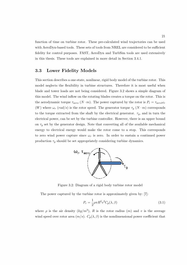
This section describes a one-state, nonlinear, rigid body model of the turbine rotor. This

model neglects the flexibility in turbine structures. Therefore it is most useful when

blade and tower loads are not being considered. Figure 3.2 shows a simple diagram of

this model. The wind inflow on the rotating blades creates a torque on the rotor. This is

the aerodynamic torque τaero (N ·m). The power captured by the rotor is Pr = τaeroωr

(W ) where ωr (rad/s) is the rotor speed. The generator torque τg (N ·m) corresponds

to the torque extracted from the shaft by the electrical generator. τg, and in turn the

electrical power, can be set by the turbine controller. However, there is an upper bound

on τg set by the generator design. Note that converting all of the available mechanical

energy to electrical energy would make the rotor come to a stop. This corresponds

to zero wind power capture since ωr is zero. In order to sustain a continued power

production τg should be set appropriately considering turbine dynamics.

Figure 3.2: Diagram of a rigid body turbine rotor model

The power captured by the turbine rotor is approximately given by: [7]:

Pr =1

2ρπR2v3Cp(λ, β) (3.1)

where ρ is the air density (kg/m3), R is the rotor radius (m) and v is the average

wind speed over rotor area (m/s). Cp(λ, β) is the nondimensional power coefficient that

22

represents how much of the power available in wind is captured. It is a function of the

blade pitch angle β (deg) and the tip speed ratio λ := Rωrv (unitless).

A one-state nonlinear model of the rigid-body rotor dynamics can be obtained using

Newton’s law for the system shown in Figure 3.2:

ωr =1

J(τaero − τg) (3.2)

where J (kg ·m2) is the combined rotor, generator and drivetrain inertia. The turbine

gearbox is ignored here. The quantities J , τaero and τg are expressed as their low-speed

shaft equivalents. Using the rotor power Pr expression from Eq. (3.1) and substituting

τaero for Prωr

in Eq. (3.2) gives:

ωr =ρπR2v3Cp(λ, β)

2Jωr− τgJ

(3.3)

Here the Cp(λ, β) data is usually available in lookup tables.

The accuracy of the one-state nonlinear rotor model depends on the size and the

flexibility of the turbine. However, for most current turbines this model can capture the

rotor dynamics accurately enough for closed-loop control purposes. We use this model

in Section 5.3 for optimal Region 2 control. A linearized version of this model is used

in Section 5.4 for optimal Region 3 control for rotor speed tracking.

3.4 Medium Fidelity Models

3.4.1 Turbine Dynamics

The Fatigue, Aerodynamics, Structures and Turbulence (FAST) turbine simulation

package [51, 55] is used to model turbine dynamics in this thesis. FAST is a pub-

licly available nonlinear aeroelastic turbine simulation code developed by the National

Renewable Energy Laboratory (NREL). FAST captures the effects of structural flexi-

bility that was ignored by the 1-state nonlinear rigid-body rotor model. FAST has been

validated against ADAMS and Germanischer Lloyd turbine simulation codes [56]. It

has been certified by Germanischer Lloyd that it is acceptable for turbine manufacturers

to use FAST for onshore turbine certification.

The tower, blades and the drivetrain are treated as flexible structures in FAST. The

drivetrain torsional flexibility is modeled as a linear inertia-spring-damper system. The

23

deflection of the tower and the blades are approximated via assumed modes method.

The properties of the tower and the blades can vary along their length. These properties

are specified at desired points on the structures. Linear interpolation is used between

these points. For instance this allows specification of different airfoil properties along

the blade length.

FAST is integrated with the AeroDyn [52] code of NREL for the calculation of

aerodynamic loads. AeroDyn uses blade element momentum theory to calculate aero-

dynamic forces and moments. Modifications and corrections are implemented for blade

tip losses and yawed wind inflow. If desired the FAST code can be coupled with other

aerodynamics tools or CFD codes instead of AeroDyn.

The FAST code can model the onshore wind turbines with a total 18 degrees of

freedom (DOF). An extra 6 DOF are available for modeling of platform motion for

offshore wind turbines. The full list of 18 DOF in FAST for 3-bladed onshore wind

turbines is as follows. 4 DOF include first and second tower bending modes in fore-

aft as well as side-to-side directions. Three degrees of freedom for each blade model

the first edgewise bending mode in addition to the first and second bending modes in

flapwise direction. These account for 9 DOF in total. Drivetrain torsion and generator

speed correspond to 2 DOF. 1 DOF accounts for the nacelle yaw motion. 2 more DOF

correspond to rotor and tail furl.

The wind field used in FAST simulations can be described in two levels of fidelity.

One option is to describe the spatial and temporal variations in the field by a combina-

tion of various time-varying parameters. These parameters are the average horizontal

wind speed over the rotor area, vertical wind speed, wind direction, vertical and hori-

zontal wind shears. The second option is the use of so-called full-field wind data. Wind

speed in three directions on a raster grid over the rotor surface is specified as a func-

tion of time. This second option allows a more realistic modeling of the wind field by

better capturing the spatial variations in the wind field. This is important for larger

commercial wind turbines where wind can vary significantly over the rotor surface. This

higher-fidelity option is used in our simulations. Wind files in both formats can be gen-

erated with the TurbSim [54] code of NREL. TurbSim has the capability of generating

wind trajectories with various spatial and temporal correlation models. These models

include common turbulence models that are used for wind turbine testing as defined in

24

the IEC-61400-1 [44] standards.

Figure 3.3: The Controls Advanced Research Turbine (CART3) at the NWTC site atGolden, CO. Photo courtesy of Benjamin Sanderse from Energy Research Centre of theNetherlands.

The turbine models we use are the 600kW 3-bladed Control Advanced Research

Turbine (CART3) and the 1.5MW WindPACT [57, 58] turbine. The CART3, shown

in Figure 3.3, is located at Boulder, Colorado at the National Wind Technology Center

(NWTC) site. The 1.5MW WindPACT is a hypothetical turbine designed by the

NWTC and Windward Engineering. The rotor diameters are 40m and 70m respectively.

The size of these turbines are representative of the currently fielded commercial turbines.

The FAST model data for the CART3 turbine was obtained from A. Wright [59]. The

model of the WindPACT turbine is distributed with the original FAST code. These

models are chosen because they are heavily used in turbine control literature.

Our medium-fidelity simulations use 15 of the 18 available DOF in FAST for onshore

25

turbines. 2 DOF for rotor and tail furl are not used since the CART3 and the Wind-

PACT turbine are designed to use active pitch control to protect turbine structures in

Region 3 operation. We also ignore the slow yaw dynamics of the turbine. The basic

FAST code does not include actuator and sensor models. In other words, the actuator

inputs affect the system immediately and the measurements are noise free. Realistic

simulations require complementing the FAST code with appropriate actuator and sensor

models. The following two sub-sections 3.4.2 and 3.4.3 discuss these actuator and sensor

dynamics respectively. The 15 DOF FAST model implemented in Simulink with these

actuator and sensor models is used as the basis of our medium-fidelity simulations.

3.4.2 Actuator Dynamics

The control inputs available for closed-loop control are the generator torque demand,

blade pitch angle demand and the turbine yaw angle demand. A model for the pitch

actuators are implemented, but the generator and yaw dynamics are ignored. This is

because the blade pitch actuators play an important role on control performance. Blade

pitch actuators have restrictive bandwidths for our turbine control problems of interest,

namely power capture optimization and structural load reduction. In addition, there

are hard bounds on pitch rates that put fundamental constraints on the achievable

performance. The dynamics of these pitch actuators can be approximated by first or

second order linear systems. In the case of the CART3 and the WindPACT turbine, first

order models are sufficient. These pitch actuator models have bandwidths of 30rad/s,

10rad/s and the pitch rate limits of 18deg/s, 10deg/s respectively. The hard bounds

on rate limits are implemented with our simulation models.

No yaw actuator models are implemented and the turbine yaw angle is held fixed

during simulations. This is because the yaw motion and the actuator dynamics have

time constants considerable larger than the other dynamics of the system. An electrical

generator model is also omitted since these dynamics are significantly faster than the

turbine dynamics of interest. Therefore it is assumed that the generator torque demand

can be achieved almost immediately for the desired control bandwidth.

26

3.4.3 LIDAR Sensor Dynamics

A detailed model of the ZephIR LIDAR [60], a commercially available continuous wave

LIDAR, is implemented with FAST for medium-fidelity simulations. A detailed LIDAR

model is important for realistic evaluation of preview controllers’ performance that we

investigate in Chapter 5. This model captures various sources wind measurement errors

inherent to the nature of the continuous wave LIDARs. The core of this model is based

on the work in Reference [61]. It is assumed that the LIDAR is mounted at the turbine

hub in a forward looking fashion and spinning with the rotor. The LIDAR itself also

contains an internal spinning mechanism that allows its laser beam to be directed in

any direction during operation independent of the rotor angle. It is assumed that the

LIDAR is supplying the average of the wind measurements at three points in space

to the controller. In other words, the spinning mechanism in the LIDAR is used to

direct the laser beam in three directions during one sample time of the controller. The

location of these three points depend on the preview time and the desired measurement

point on the blade span. We use the CART3 turbine for our preview control research.

The measurement point on each place is chosen at the 75% blade span or 15m from

the rotor hub. The future position of the blades is estimated by a constant rotor speed

assumption during the preview time. This measurement point is moved horizontally in

space for the desired preview amount. The outer section of the blades is chosen since

most of the turbine power capture is obtained around this section.

The LIDAR sensor measures a weighted average of the wind speed along its beam in

three dimensional space. The use of this model incorporates two error sources for wind

measurements. The first source of error stems from the fact that LIDAR cannot measure

wind measurements at a fixed point in space. The measurements from continuous wave

LIDARs involve a spatial weighting across the laser beam. This weighting is given by

a Lorentzian function [61]. This function depends on the focus distance. Longer focus

distances correspond to more averaging. This introduces higher errors with increasing

focus distance or preview time. The second type of error arises from the orientation of

the laser beam. The wind speed measurement of interest is the wind in the horizontal

direction at the desired blade span. A large angle between the horizon and the laser

beam means that the projection of the horizontal wind on the laser beam will be limited.

Instead, the vertical and side-wise wind speeds will corrupt the measurement. The error

27

increases with smaller preview times and measurements that are farther away in the

transverse (perpendicular to earth surface) direction from the rotor hub.

There are two more error sources that need to be considered for preview wind mea-

surements. The first source of error arises from the fact that it is not possible to know

the future rotor position. A simple predictor that assumes a constant rotor speed for the

duration of preview is used to predict the future position of the blades. This prediction

error increases with increasing preview times. The second error source is the assump-

tion of the Taylor’s frozen turbulence hypothesis, but this effect is not captured in our

medium-fidelity simulations. In other words, the evolution of the wind field from the

measurement point to the turbine is ignored. The impact of this assumption depends

on the preview time. This effect can be studied with use of an advanced computational

fluid dynamics code. However, this is beyond the scope of this study. Note that the

two error sources described in this paragraph are not directly tied to the LIDAR sensor

model.

This LIDAR model is implemented with the FAST Simulink model by reading the

full-field turbulent wind files generated by TurbSim before the simulation. These files

describe the wind speed across the rotor plane at zero yaw angle as a function of time.

This wind information is unfolded in space with the assumption of Taylor’s frozen

turbulence hypothesis [62]. It is assumed that the wind is traveling at a constant speed

which is the mean horizontal wind speed at the hub-height throughout the wind file.

FAST time-shifts the data in the full-field wind files before the simulation start time.

This is in order to contain the turbine rotor in the wind field for any initial yaw angle.

The exact time-shift in seconds is 0.5 times the ratio of the total width of the wind data

grid and the mean horizontal wind speed at hub-height [54]. This width is defined as

the size of the grid in the perpendicular direction to the vertical in the rotor plane.

3.5 Linear System Approximations

The FAST tool and many other turbine simulation tools can output linear system ap-

proximations through numerical perturbation of dynamical equations. These lower-

fidelity models allow use of well established linear control techniques. Turbine linear

models differ from the 1-state nonlinear rigid-body model and the turbine models on

28

the FAST simulation package by the fact that they are obtained numerically and not

through first principles. These linear models lose the nonlinearities captured by the

1-state nonlinear rotor model, but can capture the flexible blade and tower structural

modes. Linear models that capture the structural modes are preferred in Region 3

control since structural load attenuation is one of the main control objectives in this

region.

3.5.1 Linear Time Varying via Linearization

The nonlinear wind turbine model in FAST is represented by Equation (3.4):

q = f(q, q, u, F, t)

y = g(q, q, u, F, t)(3.4)

where q ∈ Rnq and q ∈ Rnq are the turbine states. In the most general case for offshore

wind turbines the value of nq is 24. For the utility scale onshore turbines we typically

use 15 of these 24 degrees of freedom as explained in Section 3.4.1.

It is possible disable individual degrees of freedom in FAST to obtain a lower order

nonlinear or linear model. u ∈ R5 is the control input. These inputs are the generator

torque, yaw angle and individual pitch angles for three blades. y ∈ R is the measurement

vector and its dimension depends on chosen outputs. F ∈ R7 is the wind disturbance.

This is the simplified wind field description option in the FAST simulation package.

These 7 disturbances consist of hub-height average wind speed, horizontal wind direc-

tion, vertical wind speed, horizontal wind shear, vertical power law wind shear, linear

vertical wind shear, horizontal hub-height wind gust. This simplified description is in

contrast with the more complex full-field wind description that can be used in the FAST

tool. This complex approach is not suitable for controls oriented linearization due to

high number of inputs required to the model the wind input on a raster grid on rotor.

The linearization in FAST is obtained as follows. The nonlinear system is first simu-

lated under steady wind conditions until the turbine reaches a trim operating condition.

The trim operating condition is a periodic trajectory q(t) that satisfies Equation (3.5)

¨q = f( ˙q, q, u, F , t)

y = g( ˙q, q, u, F , t)(3.5)

29

q(t) is periodic in the rotor rotation period T , i.e. q(t + T ) = q(t). The nonlinear

system (Equation (3.4)) is linearized around q(t) through numerical perturbation. The

resulting linear time-varying model have the form of Equation (3.6).

δx = A(ψr(t))δx +B(ψr(t))δu +Bd(ψr(t))δF

δy = C(ψr(t))δx +D(ψr(t))δu +Dd(ψr(t))δF(3.6)

where

δx(t) :=

[δq(t)

δq(t)

]=

[q(t)− q(t)

q(t)− ˙q(t)

]δu(t) := u(t)− u(t)

δF (t) := F (t)− F (t)

δy(t) := y(t)− y(t)

(3.7)

The dimensions of the δx(t), δu(t), δF (t), δy(t) directly follow from the state, input

and output signal dimensions from Equation (3.4) used for linearization. Since the trim

trajectories are periodic, ψr(t) = ψr(t+T ), the system equations given by Equation (3.6)

are also periodic.

It is common in turbine control literature to approximate the periodic time varying

system (PLTV) in Equation (3.6) by a time-invariant one. This is typically done to make

use of well established linear time invariant (LTI) control techniques. LPV models

built by a combination of LTI models obtained at different operating conditions are

also used in the literature. These models capture the model variations due to the

change in operating condition as defined by the mean wind speed over the rotor surface.

There are various methods to perform the LTI approximation for PLTV systems. The

simplest approaches are to evaluate the PLTV system at one rotor position or to average

the state matrices over one rotor period. These approaches ignore the periodic modal

characteristics of the turbine and typically do not provide an LTI model of sufficient

accuracy. Floquet theory [63, 64] gives a time-varying coordinate transformation that

transforms a PLTV system into one with a constant state “A” matrix. The Floquet

transformation retains the periodic modal characteristics but physical intuition about

the system states is lost in the transformed system. The most common approach for

wind turbine models is to use the multi-blade coordinate (MBC) transformation [65–71]

30

followed by averaging. We employ this approach in our multivariable controller design

work in Chapter 4. Section 3.5.2 discusses the details of the MBC transformation in

detail.

3.5.2 LTI Approximation and Multiblade Coordinate Transformation

The linear and nonlinear wind turbine equations of motion presented in Sections 3.4.1

and 3.5.1 are derived using a variety of coordinate frames. The FAST manual [51]

contains detailed figures of the coordinate frames used to derive the nonlinear turbine

equations of motion (Equation (3.4)). Specifically, the tower and rotor degrees of free-

dom are expressed in an earth fixed coordinate frame while quantities associated with

individual blades are defined in a frame that rotates with the rotor. For example, the

tip displacements of the blade flapwise bending mode are defined with respect to a

rotating coordinate frame attached to the blade. The MBC transformation takes the

system states, inputs and outputs defined in a mixed coordinate system (both rotating

and non-rotating) and expresses them in a purely non-rotating coordinate frame.

The MBC transformation was originally developed in the helicopter literature [63,

72]. It transforms quantities from rotating blade coordinates into a non-rotating, inertial

coordinate frame. The MBC transformation ideally converts the PLTV system into an

LTI system. In practice, applying the MBC to the PLTV models generated by FAST

yields a system that is still “weakly” periodic, i.e. the transformed system is periodic

but with significantly less time variation compared to the original PLTV system. An

LTI approximation is obtained by averaging the state matrices of the “weakly” periodic

system over one rotor period. This LTI approximation is of sufficient fidelity in many

cases [67]. However, the averaging step is ad-hoc and does not rely on a quantifiable

error criterion.

The MBC transformation is used to convert blade quantities back and forth between

rotating and non-rotating (inertial) coordinate frames. Define the transformation matrix

M : R → R3×3 as a function of rotor position:

M(ψ) :=

1 sin(ψ) cos(ψ)

1 sin(ψ + 2π3 ) cos(ψ + 2π

3 )

1 sin(ψ + 4π3 ) cos(ψ + 4π

3 )

(3.8)

31

For a given rotor position ψ, M(ψ) transforms quantities in the inertial (non-rotating)

frame to the rotating frame attached to the rotor. Conversely, the inverse of M(ψ)

transforms quantities from a rotating to non-rotating frame. This inverse is explicitly

given by

M(ψ)−1 =2

3

12

12

12

sin(ψ) sin(ψ + 2π3 ) sin(ψ + 4π

3 )

cos(ψ) cos(ψ + 2π3 ) cos(ψ + 4π

3 )

(3.9)

As a simplified example, consider a five DOF (on-shore) turbine model that includes

rotor position, first tower fore-aft bending mode, and first flapwise bending mode for

each blade. For constant wind conditions, this five DOF model can be specified by a

nonlinear dynamical equation of the form:

q = f(q, q, u)

y = g(q, q, u)(3.10)

where q ∈ R5 is defined as:

q :=

Tower 1st Fore-Aft Tip Displacement (m)

Rotor position, ψ (rad)

Blade 1 1st Flapwise Tip Displacement (m)

Blade 2 1st Flapwise Tip Displacement (m)

Blade 3 1st Flapwise Tip Displacement (m)

(3.11)

The rotor position, denoted as ψ, is defined to be zero when blade 1 is in the upward

position. The input and output vectors, u ∈ R4 and y ∈ R4, are defined as:

u :=

Blade 1 Pitch Angle (rad)

Blade 2 Pitch Angle (rad)

Blade 3 Pitch Angle (rad)

Generator Torque (N m)

(3.12)

y :=

Rotor Speed (rpm)

Blade 1 Root Bending Moment (kN m)

Blade 2 Root Bending Moment (kN m)

Blade 3 Root Bending Moment (kN m)

(3.13)

32

A linearization of this nonlinear FAST model yields the periodic LTV model in

Equation (3.6). In this example the last three entries of the output vector are the root

bending moments for the three blades measured in the rotating frame. For a given rotor

position ψ these quantities are transformed to the non-rotating frame by:ynravg

ynryaw

ynrtilt

=M(ψ)−1

y2

y3

y4

(3.14)

The superscript nr denotes quantities expressed in an inertial non-rotating frame. After

the transformation, these quantities have meanings in terms of rotor motion instead of

individual blades. ynravg represents average value of blade root bending moments. The

average moment causes the rotor to bend as a cone. ynrtilt and ynryaw are the blade moments

resulting in rotor tilt and yaw, respectively [17]. Similarly, the blade pitch angle inputs

and blade flapwise tip displacements can be mapped from rotating to non-rotating

coordinates: unr1

unr2

unr3

=M(ψ)−1

u1

u2

u3

(3.15)

qnr3

qnr4

qnr5

=M(ψ)−1

q3

q4

q5

, (3.16)

qnr3 , qnr4 , and qnr5 are the rotor coning, rotor tip-path-plane fore-aft tilt and rotor tip-

path-plane side-side tilt, respectively [69]. Moreover, unr1 is the collective pitch command

while unr2 and unr3 are cyclic individual blade pitch commands.

The system states, inputs, and outputs are defined in a mixed coordinate system,

i.e. they have entries expressed in both rotating and non-rotating (inertial) coordinate

frames. The MBC transformation is used to convert all quantities to a non-rotating

coordinate frame. Specifically, the transformation M introduced in Equation 3.8 is

used to define a transformation Mq acting on the linearized DOF:

Mq(ψ(t)) :=

[I2 02

02 M(ψ(t))

](3.17)

33

The linearized DOFs are transformed as:

δq(t) =Mq(ψ(t)) δnrq (t) (3.18)

Mq transforms only those quantities that are specified in the rotating frame. Quantities

specified in the inertial frame are left unchanged. Similarly, the state, input, and output

transformations for the linearized system are:

δx(t) =Mx(ψ(t)) δnrx (t) (3.19)

δu(t) =Mu(ψ(t)) δnru (t) (3.20)

δy(t) =My(ψ(t)) δnry (t) (3.21)

where the transformation matrices are given by

Mx(ψ(t)) =

[Mq(ψ(t)) 05ddtMq(ψ(t)) Mq(ψ(t))

](3.22)

Mu(ψ(t)) :=

[M(ψ(t)) 0

0 1

](3.23)

My(ψ(t)) :=

[1 0

0 M(ψ(t))

](3.24)

The transformationMx is derived by applying the chain rule to Equation 3.18 and using

the definition of δx in terms of δq and δq. The complete MBC transformation for the

linearized system is given by the collection of state, input, and output transformations

(Mx,Mu,My). Applying these transformations to the PLTV model in Equation 3.6

reduces the variation due to rotor position but it typically does not lead to an LTI

system. Averaging the remaining variations over one rotor period often gives an LTI

model of sufficient fidelity [67]. The basic approach reviewed in this section can easily

be generalized to turbine models with additional DOFs specified in the inertial and/or

rotating frames. Additional details of MBC can be found in [69] and in the manual for

the NREL MATLAB utilities that implement the MBC transformations [70].

Chapter 4

Multivariable Control Design

4.1 Introduction

Modern wind turbines are multivariable systems with multiple actuators and sensors

used to balance the competing performance objectives of power capture and load re-

duction. This challenging controller design problem is also complicated by the changes

in the nonlinear turbine dynamics and the performance objectives with the wind speed.

Controllers need to adapt to these changes based on wind speed, but an accurate wind

speed measurement is typically not available. Despite these challenges, industrial tur-

bine control is still, for the most part, based on classical, single-input single-output

(SISO) designs. Classical SISO designs have a small number of easily tunable param-

eters engineers can manipulate. Each tunable parameter has a well-understood im-

pact on the turbine performance. Thus industrial control designers can quickly tune

the controller to obtain acceptable, although sub-optimal, performance. The advanced

multiple-input multiple output (MIMO) design methodologies can deliver superior per-

formance and reduced structural loads but they tend to have significantly more tunable

design parameters. Multivariable control techniques also optimize performance with

respect to mathematical costs (H∞ norm, integral quadratic costs) that can be diffi-

cult to relate to the actual turbine performance objectives. Hence tuning of advanced

multivariable controllers can be significantly more time consuming as well as requiring

specific expertise in the particular design methodology. Advanced methodologies can

increase performance and reduce failures but at the price of increased design time and

34

35

cost, both of which are critical in an industrial setting.

There have been many research papers on advanced strategies for Region 3 control [3,

14, 17, 20, 25, 28, 43]. These research papers include a variety of methods to reduce

tower/blade bending loads and increase the drivetrain damping. Studies whose aim is to

reduce blade loads in Region 3 have mainly focused on advanced multivariable controllers

that use individual pitch control, i.e. different pitch commands are used for each of the

three blades [17,20,24,25,28]. Drivetrain dampers have been designed that account for

the cross-coupling between blade pitch and the drivetrain natural frequency [14]. The

advanced control designs have demonstrated significant performance benefits both in

simulation as well as on fielded research turbines [3, 43]. However, these methods have

not transitioned well to industry due to design time and development cost constraints.

This chapter focuses on a framework for efficient design of multivariable controllers

for industrial systems described by nonlinear dynamics. A two-layered architecture is

proposed. The lower layer uses signal-based H∞ control design, with weighted tuning

parameters, to construct multivariable controllers based on linear model approxima-

tions. The upper layer is used to specify the performance constraints and objectives

such as power capture, structural load reduction and blade pitch-rate limits. A gra-

dient optimization is used to tune the parametrized controller weighting functions in

the lower layer based on user specified performance criteria in the upper layer. This

approach combines the mathematical tractability and computational efficiency of H∞

multivariable control with the ease of design tuning for specific performance metrics on

the nonlinear plant. The proposed framework aims for fast and easy design of advanced

multivariable controllers thus speeding their transition to the industry. We use a largely

simplified Region 3 turbine control design problem to test the efficiency of the proposed

framework. For this problem the upper design layer considers important turbine design

limitations such as blade pitch rates, generator overspeed and damping of flexible modes

of the system. The lower layer tracks rotor speed and rejects wind disturbances. This

example is based on a medium-fidelity nonlinear aeroelastic simulation model. It should

be noted that this is a preliminary example that ignores the variations in the nonlinear

model and the operating-condition based control objectives. However, it still serves to

investigate the applicability of this framework on a simpler class of control problems.

The remainder of the chapter is structured as follows. Section 4.2 gives an overview

36

of the proposed design framework. The example Region 3 turbine control problem is

presented in Section 4.3. Results obtained for this example problem are discussed in

Section 4.4. Our conclusions are summarized in Section 4.5.

4.2 Multivariable Control Design Framework

This section explains the proposed design framework for tuning advanced multivariable

controllers. We propose this framework with two main objectives. The first goal is to

automate the tuning of advanced multivariable controllers. This simplifies the tuning of

the abstract design parameters and lowers the knowledge requirement for the application

of the advanced methods. The second goal is to directly incorporate the nonlinear plant

and the real performance metrics of interest to the design and tuning process. The aim

is to eliminate the iterations between linear control design and the nonlinear Monte

Carlo testing. The proposed framework can be generically applied to any nonlinear

time-varying plant, i.e. this design framework is not specific to wind turbines.

4.2.1 Problem Formulation

Figure 4.1 presents a classical feedback diagram for an industrial system. K represents

the controller to be designed and P is the plant to be controlled. The plant P can

be a nonlinear, time-varying system. Assume P is described by the following ordinary

differential equations:

x = f(x, d, u, t)

w = h1(x, d, u, t)

y = h2(x, d, u, t)

x(0) = x0

(4.1)

where t ∈ R is time. x(t) ∈ Rnx , d(t) ∈ Rnd , u(t) ∈ Rnu and y(t) ∈ Rny are the state,

disturbance, control input and measurement at time t, respectively. x(0) is the initial

condition at time t = 0. w(t) ∈ Rnw is a signal which is used to specify the performance

objectives and constraints. f : Rnx ×Rnd ×Rnu ×R → Rnx is the vector field, h1 : Rnx ×Rnd ×Rnu ×R → Rnw is the performance equation and h2 : Rnx ×Rnd ×Rnu ×R → Rny

is the measurement equation. There is a rich body of mathematical results providing

37

technical conditions which ensure the existence and uniqueness of solutions over a time

interval [0, tf ]. We assume that the vector field, measurement equation, performance

equation and initial condition are such that there exists a unique solution x ∈ Lnx2 [0, tf ],

measurement y ∈ Lny

2 [0, tf ] and performance w ∈ Lnw2 [0, tf ].

r-- K u -

d

-P

w-

y

Figure 4.1: Nonlinear, classical feedback diagram

Eq. (4.1) assumes that w(t) contains all the signals that might be used to specify

some performance constraints without loss in generality. Mathematically oriented ob-

jectives, e.g. signal L2-norm, or more complicated objectives such as damage-equivalent

loads in a turbine structure can be used. In the most general case, a performance con-

straint can be specified as a functional on w(t) that maps it to a scalar number. Let

Ci : Lnw2 [0, tf ] → R denote the functional that describes the ith performance constraint

by Ci(w) ≤ 0. In other words, Ci maps the trajectory w(t) to a scalar non-positive

number if the ith performance constraint is satisfied. Assume there are m such con-

straints and let C : Lnw2 [0, tf ] → Rm denote the vector stacking of all such constraints.

In other words, the performance constraints are denoted by C(w) ≤ 0. Similarly, let

G : Lnw2 [0, tf ] → R denote an objective function that quantifies the performance of the

output by G(w). For example, if w(t) is the bending load on the turbine tower then

the L∞ norm, G(w) := maxt|w(t)|, represents the peak bending load over time on the

turbine tower.

Denote a trim initial condition and time-varying operating trajectory with x0, d(t),

u(t), y(t) for t ∈ [0, tf ]. The control problem considered is as follows: Design a controller

K such that the feedback connection of the nonlinear, time-varying plant P and the

controller K in Figure 4.2 satisfies the performance constraints C(w) ≤ 0 when operating

close to x0, d(t), u(t), y(t). The controller K has the inputs δr = ξr(r, u, y, d, u, y) and

δy = ξy(r, u, y, d, u, y) where ξr : Rnr × Rnu × Rny × Rnd × Rnu × Rny → Rnr and

ξy : Rnr × Rnu × Rny × Rnd × Rnu × Rny → Rny . The plant input u(t) is related to

the controller output δu through u = ξu(r, u, y, d, u, y) where ξu : Rnr × Rnu × Rny ×

38

Rnd ×Rnu ×Rny → Rnu . The functions ξu, ξy and ξr represent input, measurement and

reference transformations that relate the signals in the interconnection to the control

objectives. In the standard case, these transformations simply subtract off and add

back trim conditions as would be used in most linear control designs implemented for

a nonlinear plant. The more general notation used here is to allow for other types

of transformations, e.g. the multiblade coordinate transformation in turbine control.

These transformations and objectives are selected by the designer before the design

task of K. For instance, let y(t) represent the turbine tower structural load. The

objective is to keep y(t) constant at the average of its trim trajectory over time to

minimize structural fatigue. Then the transformation ξy = y − 1T

∫ T0 y(t) dt is chosen

to represent this objective where T is the trim oscillation period. The combination of

the K, ξu, ξy, ξr corresponds to the K in Figure 4.1 where the dependency of K on

d(t), y(t), u(t) was omitted for simplicity.

ξy -δy

ξr -δr

K

-δuξu -

u

-d

P

-w

-

y

-

-

-

-

-r

-

-

Figure 4.2: Controller implementation on the nonlinear plant

Many potential issues are glossed over in this formulation. First, the controller K

may fail to satisfy the performance constraints at an initial condition far from the x0.

Second, d(t) can be a stochastic signal. The plant behavior around the deterministic

d(t) may not sufficiently capture the system dynamics for other potential trajectories.

Third, the control objectives can be a function of the disturbance d when a reliable

measurement of d is not available. This raises issues with the choice of ξr, ξu and ξy

for the implementation of the controller. Consider the turbine tower structural load

example with ξy = y − 1T

∫ T0 y(t)dt mentioned in the previous paragraph. In reality,

the control objective the average tower load depends on d. In other words, we rely on

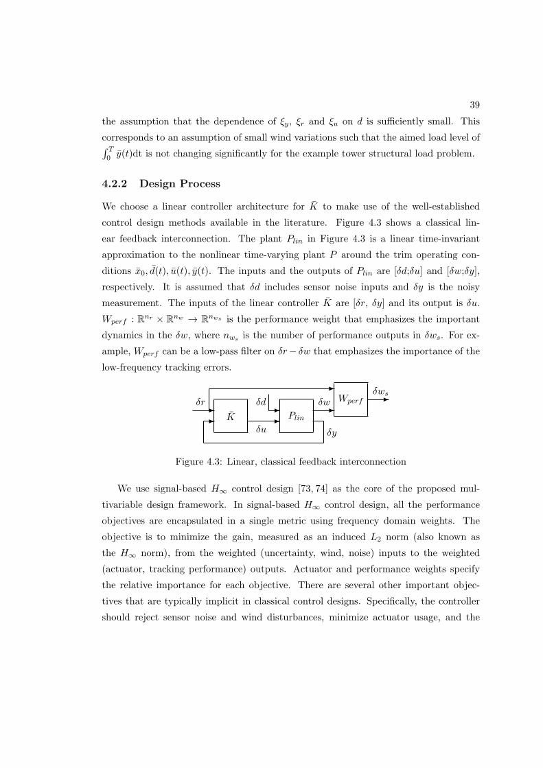
39

the assumption that the dependence of ξy, ξr and ξu on d is sufficiently small. This

corresponds to an assumption of small wind variations such that the aimed load level of∫ T0 y(t)dt is not changing significantly for the example tower structural load problem.

4.2.2 Design Process

We choose a linear controller architecture for K to make use of the well-established

control design methods available in the literature. Figure 4.3 shows a classical lin-

ear feedback interconnection. The plant Plin in Figure 4.3 is a linear time-invariant

approximation to the nonlinear time-varying plant P around the trim operating con-

ditions x0, d(t), u(t), y(t). The inputs and the outputs of Plin are [δd;δu] and [δw;δy],

respectively. It is assumed that δd includes sensor noise inputs and δy is the noisy

measurement. The inputs of the linear controller K are [δr, δy] and its output is δu.

Wperf : Rnr × Rnw → Rnws is the performance weight that emphasizes the important

dynamics in the δw, where nws is the number of performance outputs in δws. For ex-

ample, Wperf can be a low-pass filter on δr− δw that emphasizes the importance of the

low-frequency tracking errors.

δr-- K -

δu

δd -Plin

δw-

δy

Wperf

-δws-

Figure 4.3: Linear, classical feedback interconnection

We use signal-based H∞ control design [73, 74] as the core of the proposed mul-

tivariable design framework. In signal-based H∞ control design, all the performance

objectives are encapsulated in a single metric using frequency domain weights. The

objective is to minimize the gain, measured as an induced L2 norm (also known as

the H∞ norm), from the weighted (uncertainty, wind, noise) inputs to the weighted

(actuator, tracking performance) outputs. Actuator and performance weights specify

the relative importance for each objective. There are several other important objec-

tives that are typically implicit in classical control designs. Specifically, the controller

should reject sensor noise and wind disturbances, minimize actuator usage, and the

40

performance should be robust to model uncertainties.

Figure 4.4 presents a typical H∞ design interconnection. This interconnection is

used to specify the relative importance of the signals encountered in the linear system

approximation in Figure 4.3 for optimal control design. The signals in this interconnec-

tion can be categorized into four groups. The exogenous inputs are [δdu, δd, δr] where

the hat notationˆdenotes the normalized, L2 norm bounded signals. The outputs are

[δus, δws] where the subscript s denotes the weighted signals. The controller takes the

measurements [δy, δr] and outputs δu. The weights Wdu , Wd and Wr represent the

expected frequency content of the typical δdu, δd and δr signals, respectively. Similarly,

the weights Wu, Wperf represent the relative importance of the δu and δw respectively.

These weights can be either constant or dynamic. In the latter case they must be stable

and proper systems.

ControlInputs δu - +

+

InputUnc. δdu

?Wdu

? -

6Wu

6

ActuatorPen. δus

?Wd

-

Disturbanceδd

Plin δy

�NoisyMeasurements

δw -Wperf -

WeightedPerformance δws

δr�Wr

-

�ReferenceCommands δr

Figure 4.4: H∞-optimal controller design interconnection

Wd represents the expected frequency content of the exogenous disturbances and

measurement noise. Disturbance data can typically be obtained from open-loop or offline

data from the plant P . Noise information is derived from laboratory experiments or is

based on manufacturer measurements. An example is the wind disturbance experienced

by a turbine. Typically this data is available from the met towers installed for wind farm

feasibility studies at the site. Fast Fourier Transformation and power spectral density

estimation techniques can be used to extract the frequency content of this time-domain

data.

Wr is used in problems requiring tracking a reference command. It shapes the

frequency content of the expected reference signals. For example δr can be the desired

41

pitch rate command for a plane. Fighter pilots typically generate control stick inputs up

to 12rad/s. In this case Wr can have a low-pass filter characteristic with a bandwidth

of 12rad/s.

Wdu is the input uncertainty that lumps the uncertainties in the plant Plin into a

single weight. This uncertainty modeling method was chosen due to its simplicity. Since

the output of the Wdu is added to the actual control signal δu, a choice can be made

considering the expected ||δu(t)||∞ = maxt |δu(t)| and the frequencies where the model

uncertainties are large, i.e. where the dynamics of P and Plin differ largely. Wdu can be

set as dynamic weight such that its gain is a small percentage of the ||δu(t)||∞ in the

frequency range where the model uncertainties are small. A higher gain should be used

at frequencies where the model deviations in P from Plin is large. This weight limits the

frequencies where the controller will be active. Specifically, there is no control authority

when the magnitude of the uncertain input δdus is as large as the control signal δu.

This is because the uncertain, weighted signal δdus with arbitrary phase can cancel the

command from the controller.

The performance penalty Wperf can contain two types of weights. For the tracking

objectives, it can contain a desired ideal model for the closed-loop system and weigh

the difference between the ideal and the actual response. Often it is desired to have a

good match at low-frequencies within the actuator bandwidth. Wperf can also penalize

the other variables internal to the Plin that are not a part of the tracking objectives.

Wu is used to penalize the control signal usage. This is necessary to limit the actuator

use to keep them within their deflection and rate limits in the face of the tracking and

disturbance rejection objectives already defined. One choice is a high pass filter that

penalizes high-frequency control signal beyond the bandwidth of the actuators.

Denote the H∞ design interconnection with inputs [δdu, δd, δr, δu] and outputs

[δws, δus, δy, δr] as Plin. In the most general case, all such interconnections can be

represented in the linear fractional transformation form shown in Figure 4.5. The H∞-

norm of this closed-loop system is defined as [74]:

||Fl(Plin, K)||∞ = maxω

σ(Fl(Plin, K)(jω)) (4.2)

where Fl is the lower linear fractional transformation, ω is the frequency-domain vari-

able, σ is the peak singular value across all input-output channels as a function of the

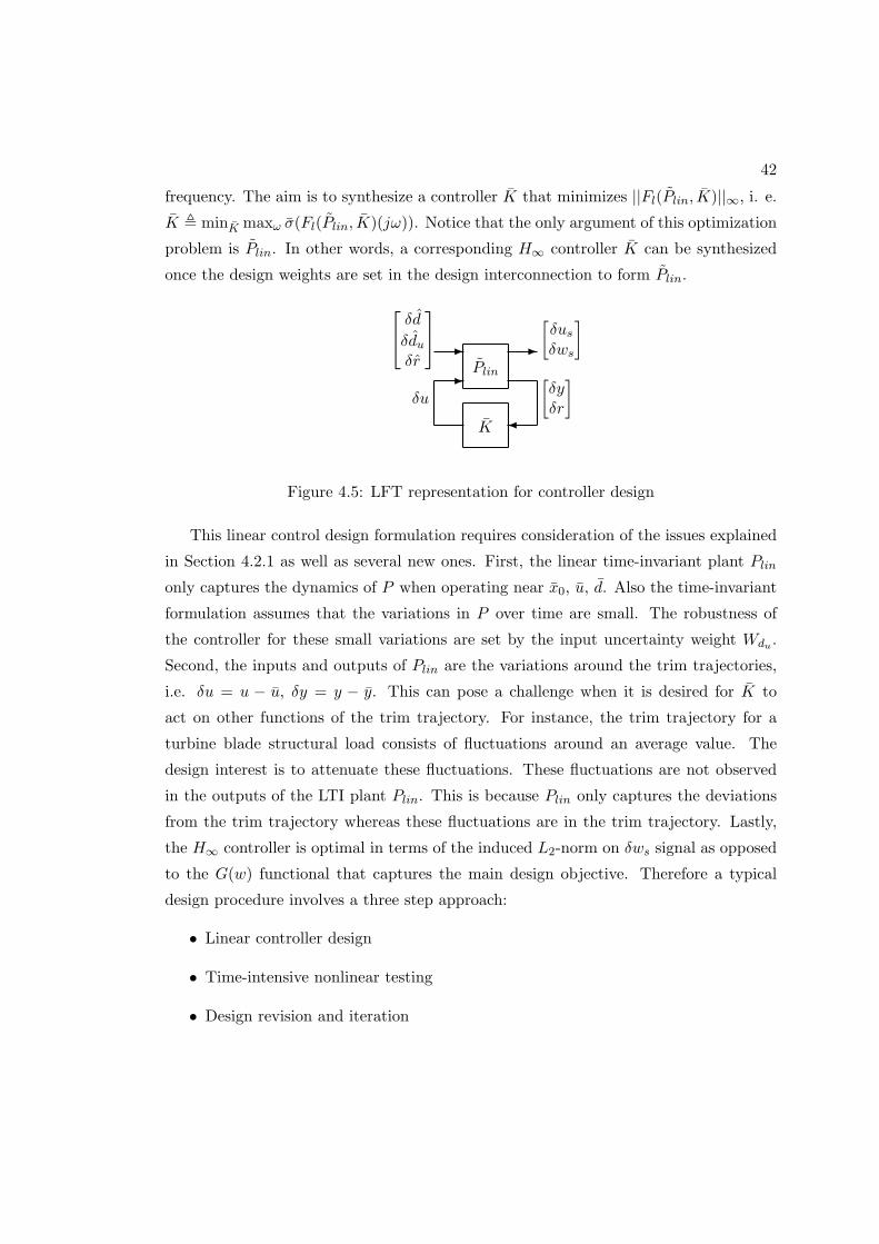
42

frequency. The aim is to synthesize a controller K that minimizes ||Fl(Plin, K)||∞, i. e.

K , minK maxω σ(Fl(Plin, K)(jω)). Notice that the only argument of this optimization

problem is Plin. In other words, a corresponding H∞ controller K can be synthesized

once the design weights are set in the design interconnection to form Plin.

Plin

K

δdδduδr

-

δu

-

[δusδws

]- [

δyδr

]�

Figure 4.5: LFT representation for controller design

This linear control design formulation requires consideration of the issues explained

in Section 4.2.1 as well as several new ones. First, the linear time-invariant plant Plin

only captures the dynamics of P when operating near x0, u, d. Also the time-invariant

formulation assumes that the variations in P over time are small. The robustness of

the controller for these small variations are set by the input uncertainty weight Wdu .

Second, the inputs and outputs of Plin are the variations around the trim trajectories,

i.e. δu = u − u, δy = y − y. This can pose a challenge when it is desired for K to

act on other functions of the trim trajectory. For instance, the trim trajectory for a

turbine blade structural load consists of fluctuations around an average value. The

design interest is to attenuate these fluctuations. These fluctuations are not observed

in the outputs of the LTI plant Plin. This is because Plin only captures the deviations

from the trim trajectory whereas these fluctuations are in the trim trajectory. Lastly,

the H∞ controller is optimal in terms of the induced L2-norm on δws signal as opposed

to the G(w) functional that captures the main design objective. Therefore a typical

design procedure involves a three step approach:

• Linear controller design

• Time-intensive nonlinear testing

• Design revision and iteration

43

The design revision step relies on designer’s knowledge about the plant and the chosen

control method. This iteration continues until satisfactory performance is achieved in

the nonlinear testing step. This iterative approach increases design time and cost.

4.2.3 Auto-Tuning Framework

There is a correspondence between the generalized plant Plin and K, i.e. given a Plin

an H∞ optimal K can be synthesized. This correspondence can be used to formulate

a finite-dimensional nonlinear control problem that optimizes K based on performance

requirements C(w) ≤ 0 and objectives G(w) specified in the time and frequency do-

mains. The weights used to construct the generalized plant Plin can be parametrized

for tuning. As an example, block diagonal weights are used to penalize each actuator

and performance penalty signal independently. Each weight is parametrized as:

W (s) = F0(1 + γ1)s+ z0(1 + γ2)

s+ p0(1 + γ3)(4.3)

where F0, z0, p0 are the initial gain, location of the zero and the pole of this 1st order

weight. γ1, γ2, γ3 represent percentage-wise adjustments made by the optimization. Let

γ ∈ Rnγ be the vector of the parameters of Wu and Wperf that appear in the H∞

architecture. For each set of weight parameters γ, a controller, denoted Kγ(s), can be

easily computed using standard robust control software tools [75]. This formulation

requires a strict lower-bound of −1 on each element of γ. This ensures the stability of

the weights assuming that the initial parametrized weight is stable and minimum-phase.

The nonlinear optimization problem is formulated as follows:

minimize:γ

G(wγ)

subject to: C(wγ) ≤ 0

lb ≤ γ ≤ ub

Equation (4.1)

Kγ , minK

maxω

σ(Fl(Plin(γ), K)(jω))

u = ξu(r, Kγ [δr; δy], y, d, u, y)

δy = ξy(r, u, y, d, u, y), δr = ξr(r, u, y, d, u, y)

Given x(0), r[0, tf ] and d[0, tf ]

(4.4)

44

where γ ∈ Γ ⊆ Rnγ is the allowable set of decision variables that are used to construct

an advanced, multivariable controller Kγ . Maximization problem is without loss of gen-

erality since minγ G(wγ) = −maxγ [−G(wγ)]. The subscript γ in Kγ and wγ denotes

their dependence on γ. The design task is to synthesize a Kγ that satisfies the per-

formance constraints specified in C(wγ) ∈ Rm. The Kγ is optimized with respect to

the performance objective functional G(wγ) ∈ R. The G(wγ) and C(wγ) depend on

wγ(t), which depends on Kγ , P , r, d and the initial conditions x(0). In other words,

given a set of decision variables γ an H∞-optimal controller Kγ is designed using the

generalized plant Plin(γ). The nonlinear plant P is simulated with the Kγ with the

transformations ξu, ξy, ξr for the initial condition x(0) and the disturbance trajectory

d(y). The resulting w(t) trajectory is used to evaluate the performance objective G(wγ)

and constraints C(wγ). The gradient based algorithm tunes the design parameter γ

based on G(wγ) and C(wγ) iteratively.

An initial feasible set of decision variables γ that satisfy constraints C(wγ) ≤ 0 and

bounds lb ≤ γ ≤ ub, is required. This is a common requirement of the constrained

nonlinear optimization solvers. The following iterative Phase I optimization procedure

can be followed to obtain an initial feasible point:

1. Choose a random parameter set or some intelligent heuristic based set of param-

eters on a few performance specifications such as controller bandwidth. This set

of parameters will yield an H∞ controller that stabilizes the LTI plant Plin under

some certain mild conditions [74].

2. Simulate the closed-loop nonlinear simulation with the H∞ controller obtained in

Step 1. In case the nonlinear closed-loop system is unstable skip to Step 3. If the

nonlinear closed-loop system is stable and the simulations achieve a finite cost,

continue with the Phase I optimization given in Eq. (4.5). The optimization in

Eq. (4.5) minimizes the slack variable ζ to obtain a set of design parameters γ

that easily satisfies design constraints in C(wγ).

minimize:γ,ζ

ζ

subject to: C(wγ) ≤ ζ

Other constraints in Eq. (4.4)

(4.5)

45

3. Scale down the disturbances (wind gusts and measurement noise) to a sufficiently

small level that the nonlinear closed-loop system is stable and the simulations

achieve a finite cost. Specifically, the scaled disturbance signal is d = Λ(d− d)+ dwhere Λ ∈ (0, 1] is the scale factor. At this point the H∞ controller stabilizes the

nonlinear closed-loop system for smaller amplitude perturbations from the trim.

Solve the optimization in Eq. (4.6) until Λ = 1. This yields an H∞ controller that

stabilizes the nonlinear system on the desired disturbance signals. The Phase I

optimization in Eq. (4.5) can be used at this point to find a feasible design.

maximize:γ,Λ

Λ

subject to: C(wγ) ≤ ∞

Other constraints in Eq. (4.4) where d is replaced with d

(4.6)

This problem formulation makes no assumptions about the objective functional

G(wγ), constraint functional C(wγ), or how the parameter vector γ enters into the

system dynamics and measurement equation. Consequently, this minimization is a

computationally difficult problem to solve. In general, it is not a convex optimization

and it may have many local optima that are not global optima. Our goal will be to use

gradient-based optimization to find a parameter vector that achieves a local maxima.

This will generally not find a global maxima. However, it does provide a means to

improve upon a ‘bad’ initial control design. The gradient based solver approximately

requires nγ + 1 nonlinear simulations at each iteration. The total number of simula-

tions can be approximated by nit(nγ + 1) where nit is the number of iterations. If the

computation time for one simulation is tsim then the expected time for the optimization

can be approximated with tsimnit(nγ + 1). Assuming that the tsim is approximately

independent of the decision variables, it can be calculated with a simulation before the

optimization. Therefore the total design time or the desired number of iterations can

be chosen beforehand.

4.3 Example Problem: Turbine Region 3 Controllers

This section presents an example of the proposed control design framework. A turbine

control problem in above-rated wind speeds (Region 3) is considered. We present a

46

simplified problem. Design of a controller that will be implemented on an actual tur-

bine requires many extra design considerations. However, this example still serves to

demonstrate the applicability of the proposed framework.

Typical Region 3 control design objectives consist of rotor speed regulation as well

as blade, tower and gearbox structural load minimization goals. These are disturbance

rejection goals and there are no reference tracking objectives. A major performance

constraint is to keep the generator speed under its over-speed limit. Structural load

specifications include peak load and damage equivalent loads (DELs). These perfor-

mance objectives must be satisfied under model uncertainties and limitations of the

pitch actuators. Specifically, pitch actuators have a limited bandwidth and they are

subject to pitch-rate constraints.

The nonlinear plant considered is the WindPACT 1.5MW turbine. A model of this

plant, P , is distributed with the FAST [51] aeroelastic turbine simulation package. P

includes first-order linear models of the pitch actuators that have a 10rad/s bandwidth.

The disturbance, d(t) ∈ R4, is the turbulent wind conditions that are generated by

NREL’s TurbSim [54]. A single 450s wind trajectory with 18m/s average hub-height

wind speed and 5% turbulence was chosen for Region 3 operation. This corresponds to

a typical, mild turbulence level. We use the simplified wind field description in FAST

that consists of variations in average horizontal wind speed over the rotor area (m/s),

vertical wind speed (m/s), wind direction (deg) and a constant vertical power-law wind

shear of 0.2 (unitless). The control input u(t) ∈ R3 is the pitch angle command for each

blade in (rad/s). The generator torque is held constant at its rated value of 8376.58Nm

and is not included in u(t). The plant measurements y(t) ∈ R6 consist of rotor position

(rad), rotor speed (rpm), flapwise root bending moment for each blade (kNm) and

the tower bending moment at root in the fore-aft direction (kNm). The variables used

for the performance constraints and objectives, w(t) ∈ R6, are chosen to be the same

with the vector y(t). Ideal measurements with no noise are used in simulations of P .

The following section, Section 4.3.3, explains the linearization process to obtain an LTI

turbine model Plin as well as the ξu, ξy input-measurement transformations used to

select the controller inputs and outputs.

47

4.3.1 Linear Model and Input-Measurement Transformations

Assume a constant wind speed trim operating condition d ∈ R4 where the only nonzero

elements of the disturbance vector are the average horizontal wind speed over the rotor

area 18m/s and the constant vertical power-law wind shear of 0.2 (unitless). Let u

be the corresponding constant pitch angle for trim. The turbine is subjected to time-

varying loads even in constant wind conditions because persistent disturbances such

as tower shadow, gravity and aerodynamic forces depend on the rotor position and

structural flexibility. As a result, the wind turbine trim values are time-varying and

periodic even in constant wind conditions. In other words, y(t) ∈ R6 is a periodic

trim trajectory with period T = 2π2.15 = 2.92s where 2.15rad/s is the rated rotor speed.

The value of u = 0.335rad is calculated through FAST through an iterative method.

Linearizations computed around d, u, y at various rotor positions result in a periodic,

linear time-varying (LTV) system with period equal to the rotor rotation period. The

inputs [δd; δu] and the outputs [δw; δy] of this periodic LTV are the deviations from

their respective trim trajectories. For design simplicity we eliminate 3 elements of δd

and only leave the variations in average horizontal wind speed over the rotor area (m/s)

in the linear model. This is the input channel with the largest variations and it has the

most impact on the outputs.

The multiblade coordinate transformation (MBC) followed by averaging is used to

obtain an LTI approximation from the periodic LTV model. The details of this approach

can be found in Section 3.5. The MBC transformation expresses the turbine variables

that are defined in rotating coordinate frames in a non-rotating coordinate frame. This

LTI approximation of the periodic LTV system is shown in Figure 4.6 and denoted as

Plin. ψr(t) denotes the trim trajectory of the rotor position that is contained in y(t).

Mu(ψr) : R3 → R3 and T−1y (ψr) : R6 → R6 are the MBC transformation functions. The

input transformation Mu(ψr) is given in Eq. (4.7):

Mu(ψr(t)) =

1 cos(ψr(t)) sin(ψr(t))

1 cos(ψr(t) + 2π/3) sin(ψr(t) + 2π/3)

1 cos(ψr(t) + 4π/3) sin(ψr(t) + 4π/3)

(4.7)

The measurement transformation T−1y (ψr) can be written with the help of the inverse

48

of the Mu:

M−1u (ψr(t)) =

1

3

1 1 1

2 cos(ψr(t)) 2 cos(ψr(t) + 2π/3) 2 cos(ψr(t) + 4π/3)

2 sin(ψr(t)) 2 sin(ψr(t) + 2π/3) 2 sin(ψr(t) + 4π/3)

(4.8)

T−1y (ψr(t)) =

1 0 01×3 0

0 1 01×3 0

03×1 03×1 M−1u (ψr(t)) 03×1

0 0 01×3 1

(4.9)

The superscript nr notation for δunr, δynr, δwnr denotes the quantities expressed

in non-rotating frame. More specifically, the transformed control input is δunr =

[δβcoll; δβtilt

; δβyaw ]. The δβcoll(rad) is the collective pitch angle. It is the average pitch

angle from the three blades. The δβtiltand δβyaw (rad) correspond to cyclic blade pitch

motions that control the tilting and yawing motion of the turbine rotor, respectively.

The only elements of the δy that are transformed to the non-rotating coordinate frame

are the 3rd through 5th elements. These transformed variables are δMavg , δMtilt, δMyaw .

δMavg is the average bending loads on the three blades (kNm) that cause the rotor to

assume a cone shape. The δMtiltand δMyaw (kNm) are bending moments at the root

that cause the rotor to tilt and yaw.

δd -δunr -Mu(ψr)

δu-δx = A(ψr)δx+B(ψr)δu+Bd(ψr)δd

δy = C(ψr)δx+D(ψr)δu+Dd(ψr)δd

Periodic LTV Model

-δwT−1y (ψr) -δwnr

-δyT−1y (ψr) -δynr

Approximate LTI Turbine Model

Figure 4.6: MBC application and Approximate LTI Turbine Model

In summary, the input and measurements of the nonlinear plant P and the linear

turbine model Plin are related through the transformations u =M−1u (ψr(t))δu

nr+u and

δynr = T−1y (ψr)(y(t) − y(y)). However, there are two implementation challenges with

49

this approach. First, the MBC transformation is a function of the trim trajectory of

rotor position. When implemented, the rotor position of the actual turbine will diverge

from its trim trajectory due to varying wind conditions. Hence it is desired to use the

actual rotor position, i.e. T−1y (ψr) rather than T−1

y (ψr), for the MBC transformation.

Second, it is desired from the controller to attenuate the variations around the average

of the y(t) over time in each channel. This is especially important for the bending load

measurements. Therefore the actual implementation of the transformations are u =

ξu(δunr, y, u) =M−1

u (ψr(t))δunr+ u and δynr = ξy(y, y) = T−1

y (ψr)(y(t)− 1T

∫ T0 y(t) dt).

4.3.2 H∞ Design Interconnection and the Initial Design

Figure 4.7 shows the system interconnection used for the disturbance rejecting con-

troller design. The design task is to select weights in the H∞ design interconnection in

Figure 4.7 to satisfy performance specifications on the nonlinear turbine model. These

weights can be separated into two categories. The weights Wd, Wnoise and Wdu are

selected to describe the frequency content of the wind disturbances, sensor noise and

model uncertainties. These quantities are set by the turbine design and the environ-

mental conditions. These weights are set a-priori and left as constants in the nonlinear

optimization. The second class of weights consist of Wu and Wperf . These weights

describe the actuator limitations and the performance trade-off between multiple objec-

tives. Tuning of these weights to achieve the desired performance and robustness can

be time consuming and it requires specific domain expertise in the H∞ design method-

ology. This increases both the design time and costs. Therefore this task is left to the

proposed automated tuning framework.

We aim to obtain an initial design that satisfies design constraints C(wγ) ≤ 0 in a rel-

atively small amount of time. Optimality with respect to cost function is not considered.

The resulting controller is likely sub-optimal but will be tuned by the gradient-based

optimization based on design specifications in the objective and constraint functions

G(wγ) and C(wγ).

Wd represents the frequency-content of the worst-case wind conditions for the turbine

operation. This can be obtained either from wind turbulence models appropriate for the

turbine location or from time-domain data that is gathered at the wind farm. Available

time domain data can be mapped to the frequency domain via the Discrete Fourier

50

ControlInputs δunr

- +

+

InputUnc. δdu

?Wdu

? -

6Wu

6

ActuatorPen. δunr

s

?Wd

-

Wind δd1

LTITurbineModel Plin

Outputs

- Wperf -WeightedPerformance δws

δw

?+

+� Wnoise��Measurements δy

SensorNoise δd2

Figure 4.7: System Interconnection for H∞ Region 3 Controller Design

Transform. The frequency domain magnitude data can then be over-bounded by a

transfer function to obtain Wd. For this study, operation under a mild turbulence level

(5%) is considered. Wind data with 5% turbulence with an average wind speed of 18m/s

is generated using TurbSim [54] developed by NREL. A transfer function is obtained as

described from the hub-height wind data. The resulting weight is given by:

Wd = 0.25s/60 + 1

s/4 + 1(4.10)

Wn represents the noise on the sensors. We choose Wn as constant block diagonal

weights that correspond to the 1% of the y. This approximately models noise with

amplitude equal to 1% of each signal.

The input uncertainty Wdu is chosen based on the expected peak pitch angle input

of 0.5rad. For the sake of simplicity in the example problem a constant and low level of

uncertainty, a block diagonal weight with the 2% of the trim pitch inputs, is chosen. A

more detailed uncertainty modeling approach can involve modifying the parameters of

the nonlinear model and obtaining many linearizations. An uncertainty set that covers

all these linearizations can be used.

The actuator and performance penalty weights, Wu and Wperf , are tuned by the

optimization algorithm. The initial values of these weights are chosen to obtain a

conservative controller with limited bandwidth. The block diagonal actuator penalty

weight Wu = diag(Wcoll,Wtilt,Wyaw) consists of penalties on the collective and cyclic

pitch action. These penalties are chosen as 1st order high-pass filters to penalize high-

frequency control action. Specifically, the zero locations of these filters are chosen

51

at the bandwidth of the actuator models to penalize actuation beyond the actuator

bandwidth. The gain of Wcoll is selected to be lower than the cyclic pitch penalties.

Hence the resulting controllers focus on collective pitch control. Collective pitch action

has a dominant role in rotor speed tracking and tower fore-aft bending. In addition,

this prevents controllers from using excess pitch-rates with individual pitch control.

Therefore this selection is helpful for satisfying the constraints in C(wγ) even though

it may be sub-optimal for blade load reduction. All three weights have zeros at s = 10

and poles at s = 80. Their DC (low-frequency) gains are 0.25, 1 and 1 respectively.

The block diagonal performance weight Wperf consists of weights on rotor speed

error (Wpωr), collective blade bending moments (WpMavg), blade bending moment in

tilt and yaw directions (WpMtilt and WpMyaw) and the tower fore-aft bending moment

at the tower root (WpTFA). All these weights are parametrized as 1st order transfer

functions except the penalty on the tower fore-aft bending moments. This weight was

chosen as a constant since it is sufficient to penalize its sharp peak without imposing

significant penalty at other frequencies. All 1st order weights are initially set to have

the same pole/zero location. The pole is set to be at very low frequencies (s = 0.05)

to obtain a low bandwidth controller. The location of this pole was set such that the

performance penalties roll-off before all of the turbine flexible modes. The location of

the zero s = 80 is set more than 1 decade away to keep the penalties at high-frequencies

small enough. The gains of each penalty were adjusted quickly after a few iterations

on nonlinear simulation to ensure that the controller is focused on rotor speed tracking

and tower load reduction. The gains used for the initial design for each performance

weight are 0.25, 10−4, 10−4, 10−4, 2× 10−6 respectively.

For fixed operating conditions, the H∞ weight parameters can be tuned by solving

the optimization in Equation 4.4 using gradient-based optimization methods [76, 77].

The cost and constraint functions in this optimization that depend on the weight pa-

rameters and can be evaluated as follows. The controller Kγ is constructed for a given

parameter vector γ. The turbine performance is simulated on medium-fidelity non-

linear models for a fixed set of conditions (noise, wind, and model errors) to obtain

the captured power and bending loads as a function of time. Performance constraints,

e.g. actuator position and rate limits, can similarly be formulated and evaluated in the

constraint C(wγ) ≤ 0. This optimization will return local but not necessarily globally

52

optimal parameters. The operating conditions include the wind and sensor noise profiles

as well as modeling errors. These are stochastic quantities and hence the cost and con-

straint functions are actually random values depending on the wind/noise realizations.

Stochastic optimization techniques are applicable but, for simplicity, the cost and con-

straint functions are evaluated by sufficiently long simulations that capture a sufficiently

rich set of wind variations. More realistic design tasks can contain many different real-

izations of the turbulent wind trajectories as well as the extreme operating conditions

that the turbine need to withstand. This more realistic approach is important to obtain

statistically meaningful results and to reach conclusions about safe turbine operation.

The following control problem is studied: blade damage equivalent load minimization

subject to limits on generator speed, blade pitch-rate and the damping of the tower fore-

aft motion. This problem is studied for various blade pitch-rate limitations to test the

applicability of the proposed framework. This problem also allows gaining insight into

actuator limitations and performance trade-offs. Details of the performance objective

and constraint cost and constraint functions are explained in Section 4.3.3.

4.3.3 Cost and Constraint Functions

The performance objective G(wγ) captures blade load reduction performance in terms

of damage equivalent loads. Given a controller Kγ that is a function of decision variables

γ, a medium-fidelity model of the turbine is simulated in the FAST simulation package.

Time traces of the blade bending moments are processed with MCrunch [78] developed

by NREL to obtain damage equivalent loads (DELs). G(wγ) is computed by averaging

the DELs from the three blades. Damage equivalent loads are a complex, nonlinear

cost function. DELs are non-integrable and need to be calculated after the simulation

is completed.

The performance constraint C(wγ) ≤ 0 is based on the turbine component specifi-

cations and operating conditions. The vector valued constraint functional C(wγ) has

the following structure:

C(wγ) :=

||ωγ ||∞ −D1

||βγ ||∞ −D2

||Tγ ||∞ −D3

(4.11)

53

where T is the transfer function from wind speed input to tower fore-aft motion. D1 is

the overspeed limit, D2 is the pitch rate limit, and D3 is the open-loop peak magnitude

of T . The first two entries are functions of time and for these signals || · ||∞ denotes

the peak value in time. The third entry is a transfer function and || · ||∞ denotes the

peak magnitude of the frequency response. The numerical values of the D1 and D3 are

2.252rad/s and 83.3dB respectively. This problem is solved for D2 = 6, 8 and 10deg/s

to gain insight into blade pitch rate versus performance trade-offs.

The first constraint, ||ωγ ||∞ − D1 ≤ 0, is keeping the generator speed under its

overspeed limit. An overspeed event should be avoided at all times since it can lead to

physical damage in the generator components. This requires the controller to success-

fully attenuate large gusts observed in Region 3 operation. The equivalent rotor speed

to this generator overspeed limit is D1 = 2.252rad/s for the WindPACT turbine. This

corresponds to a 0.105rad/s deviation from the trim rotor speed.

The second constraint, ||βγ ||∞ − D2 ≤ 0 , is the pitch rate bounds of the pitch

actuators. This limitation is due to the large inertia of the turbine blades and the forces

acting on them. Pitch rate limits are enforced in the nonlinear optimization through

C(wγ), but these hard bounds are not implemented in the FAST simulation model of

the WindPACT. This was done to avoid introducing a non-smooth constraint for the

generic gradient based optimization algorithm.

The third constraint of interest, ||Tγ ||∞ −D3 ≤ 0, is the damping of the tower fore-

aft motion. Tall, slender turbine towers lead to a very lightly damped flexible mode.

This design choice is made for reducing the material and transportation costs. The

frequency of this flexible mode is adjusted at design time such that it is above the rated

rotor speed, but below three times of this value for 3-bladed turbines. This is done for

avoiding the rotor rotation and the blades passing in front of the tower exciting this

flexible mode. This mode can most easily be observed in open-loop Bode plots from wind

disturbances to tower fore-aft motion as a sharp peak at the tower natural frequency.

The peak gain (infinity-norm) of this transfer function is related the damping of the

tower fore-aft bending mode. It is assumed that the turbine is operating under mild

turbulent conditions (5%) and no extra damping is demanded from the controller for

this study. However, the infinity-norm of this transfer function is constrained to be less

than or equal to the infinity-norm of open-loop response, D3 = 83.3dB. This constraint

54

prevents the control design from reducing blade loads at the expense of excessive tower

loads.

4.3.4 Gradient-based Optimization

This nonlinear optimization problem is solved with the commercially available software

MATLAB Optimization Toolbox [79] via active-set methods. This optimization is re-

peated for three different pitch rate limits. The inputs of the gradient-based algorithm

are the design constraints and a set of initial weights. A total of nγ = 19 decision vari-

ables are used in the optimization. The actuator penalty weight consists of collective

and cyclic pitch input penalties. The two cyclic pitch inputs use the same weight. The

resulting two first-order weights require 6 decision variables. Four first-order weights

and a static gain weight in the performance penalty weight require 13 decision variables.

Controllers are evaluated on a 450s wind trajectory on the FAST simulator to calculate

the cost and constraint functions. The resulting controllers are not necessarily globally

optimal. However, these results can give rough guidelines on the trade-offs between

pitch-rate limits and performance objectives. This is because all optimization problems

start from the same initial design and the only difference is the relaxation of the pitch

rate constraints.

4.4 Example Problem Results

This section presents the analysis of the resulting H∞ controllers and simulations. The

gradient-based solver took 12 iterations and 250 function evaluations, i.e. simulations,

on average before converging to an optimal point. The number of function evaluations

are approximately in agreement with the nit(nγ + 1) prediction with nγ = 19. The

final values of the cost function and the constraint functions are listed in Table 4.1.

The first column of this table lists the pitch-rate limits specified in the gradient-search

algorithm. The second column lists the final value of the cost function, i.e. average of

the DELs from three blades. The third, fourth and fifth column present the values of

the vector valued constraint function. The entries of this function are described in the

previous section. Being close to 0 from below means that the final solution is close to

the limits of the constraint. These columns are given in the units of rad/s, deg/s, dB

55

respectively. The fifth column represents the infinity norm of the wind to tower fore-aft

motion. For example a value of −6dB means the peak gain of the closed loop with

the resulting controller is 6dB less than the open loop response. The main observation

from this table is that all solutions are similarly constrained by the rotor over-speed

and blade pitch rate limits. Increasing the allowed pitch rate has a significant impact

on the achieved blade load reduction levels.

Table 4.1: Optimization Results

G(wγ) C(wγ)

D2 Blade DEL ||ωx||∞ −D1 ||βx||∞ −D2 ||Tx||∞ −D3

(deg/s) (kNm) (rad/s) (deg/s) (dB)

6 326 -0.0186 -0.112 -6.7928 288 -0.0230 -0.014 -5.14710 255 -0.0131 -0.098 -6.629

Closed loop Bode plots from wind perturbations to rotor speed errors are given in

Figure 4.8. The blue solid line is the open loop response and the green solid line is the

closed loop with the initial controller. The red dotted line, cyan dash-dotted line and

black dotted line represent the response with the final controllers obtained from gradient-

based tuning with 6, 8 and 10deg/s pitch rate limits respectively. At frequencies lower

than 0.2rad/s the initial controller and the 6deg/s pitch-rate controller have higher

attenuation. In the range of 0.2 to 10rad/s, the 8deg/s and 10deg/s controllers have

higher attenuation. The worst case amplification in this plot is much smaller for these

controllers. However, note that in Table 4.1 all controllers have a peak tracking error

(||ωx||∞−D1) that is very close to the overspeed limit. This behavior can most likely be

explained by the fact that all controllers show similar behavior beyond 10rad/s. This is

the bandwidth of the pitch actuators of the WindPACT 1.5MW turbine. Moreover, the

low-pass performance weight on rotor speed tracking errors rolls-off before this frequency

for all controllers. Therefore the increased pitch rate limits have a limited impact on

the peak tracking error caused by the wind gusts.

Three plots can be used to analyze the controller behavior and the impact of the

extra pitch rates on blade load reduction. Figures 4.9 and 4.10 present the Bode plots

from wind perturbations to collective blade bending moments and the rotor-tilt moment.

Power spectral densities (PSD) of the collective and tilt bending moment signals from

56

10−1

100

101

−50

−40

−30

−20

−10

0

10From: HH Wind Disturbance [m/s] To: RotSpeed (rpm)

Ma

gn

itu

de

(d

B)

Bode Diagram

Frequency (rad/s)

Open Loop

Closed−Loop w/ Initial H∞

CLP Final H∞ 6

° Pitch−Rate Lim.

CLP Final H∞ 8

° Pitch−Rate Lim.

CLP Final H∞ 10

° Pitch−Rate Lim.

Figure 4.8: Bode plot from wind perturbations to rotor speed error.

the FAST simulations are presented in Figure 4.11. These signals are obtained by

applying the MBC transformation to the root bending moments from three blades.

The PSD plot is important to investigate the behavior of the proposed framework by

connecting the nonlinear performance metrics with the linear system analysis via Bode

plots. The plots for the moments in the yaw direction are not presented since they had

similar trends to the moments in the tilt direction. Figure 4.11 shows that the largest

portion of the collective loads occur below 1rad/s. The controller with 8deg/s pitch

rate improves attenuation over the 6deg/s controller up to 1.5rad/s in the collective

moment Bode plot in Figures 4.9. The 10deg/s controller improves this attenuation

further. These are consistent with the PSDs in Figure 4.11. Figure 4.11 also shows

that the largest portion of the tilt loads are seen below 2rad/s with an additional peak

around 6.45rad/s. This is three times the rated rotor speed. In this channel there is

a large difference between the 6deg/s and 8deg/s controller. The 10deg/s controller is

slightly worse than the 8deg/s controller. This is also seen in the tilt channel Bode plot

in Figure 4.10. However, the peaks in the collective loads’ PSD is much higher than

the peaks in the tilt channel. Therefore this worse performance in this channel is less

important. The extra 2deg/s pitch rate limit over the 8deg/s is used in the collective

57

bending channel. As seen in the Table 4.1 the 10deg/s controller is able to achieve a

10% smaller blade DEL over the 8deg/s controller by focusing on these collective loads.

These loads are caused by the wind fluctuations that cover a large enough area to

impact the three blades simultaneously. The optimization algorithm is seen to optimize

the controller in accordance to the nonlinear simulation outputs and the performance

metrics.

10−1

100

101

15

20

25

30

35

40

45

50From: HH Wind Disturbance [m/s] To: Rotor (hub) loading (kN·m)

Magnitude (

dB

)

Bode Diagram

Frequency (rad/s)

Open Loop

Closed−Loop w/ Initial H∞

CLP Final H∞ 6

° Pitch−Rate Lim.

CLP Final H∞ 8

° Pitch−Rate Lim.

CLP Final H∞ 10

° Pitch−Rate Lim.

Figure 4.9: Bode plot from wind perturbations to collective blade bending moments.

The Bode plot for the tower fore-aft bending mode is shown in Figure 4.12. There

is a good correlation between pitch-rate limits and tower load attenuation even though

tower loads were not explicitly penalized. This is also intuitive because collective root

bending moments Mavg have an interpretation in terms or rotor hub loading, which in

turn affects forces at the tower top. Therefore improvements at Mavg attenuation are

correlated with attenuation of the tower fore-aft bending moments. This can be seen by

comparing the Bode plots in Figure 4.12 and 4.9. In both figures the 8deg/s controller

improves attenuation over the 6deg/s controller up to 1.5rad/s frequency range. The

8deg/s controller is slightly worse up to 5rad/s. At higher frequencies both controller

perform similarly. The 10deg/s controller is better than both controllers up to 10rad/s

and perform similarly beyond this frequency. The similar control behavior beyond

58

10−1

100

101

−20

−10

0

10

20

30

40

50From: HH Wind Disturbance [m/s] To: Rotor flap moment in tilt direction (kN·m)

Ma

gn

itu

de

(d

B)

Bode Diagram

Frequency (rad/s)

Open Loop

Closed−Loop w/ Initial H∞

CLP Final H∞ 6

° Pitch−Rate Lim.

CLP Final H∞ 8

° Pitch−Rate Lim.

CLP Final H∞ 10

° Pitch−Rate Lim.

Figure 4.10: Bode plot from wind perturbations to blade bending moments in tiltdirection.

0 1 2 3 4 5 6 70

1

2

3

4x 10

4 Power Spectral Density

Co

llective

Bla

de

Lo

ad

s

Frequency (rad/s)

0 1 2 3 4 5 6 70

500

1000

1500

2000

Bla

de

Lo

ad

s in

Tilt

Dire

ctio

n

Frequency (rad/s)

Closed−Loop H∞ 6

° Pitch−Rate Limit

Closed−Loop H∞ 8

° Pitch−Rate Limit

Closed−Loop H∞ 10

° Pitch−Rate Limit

Figure 4.11: Power spectral densities of the blade bending moments in non-rotatingcoordinates.

59

10rad/s is shared in all channels and is likely due to the pitch actuator bandwidth.

10−1

100

101

20

30

40

50

60

70

80

90From: HH Wind Disturbance [m/s] To: Tower base Fore−Aft moment (kN·m)

Magnitude (

dB

)

Bode Diagram

Frequency (rad/s)

Open Loop

Closed−Loop w/ Initial H∞

CLP Final H∞ 6

° Pitch−Rate Lim.

CLP Final H∞ 8

° Pitch−Rate Lim.

CLP Final H∞ 10

° Pitch−Rate Lim.

Figure 4.12: Bode plot from wind perturbations to tower fore-aft bending.

4.5 Conclusions and Recommendations

The simple example problem used to test the basic effectiveness of the proposed frame-

work showed some preliminary promising results. Particularly, it was seen that the

framework was able to tune the advanced multivariable H∞ controllers to improve the

performance of a nonlinear plant in terms of a non-integrable and non-smooth perfor-

mance metric.

The proposed framework can help transition MIMO tools to industry, but reaching

a more concrete conclusion requires further research. Some of the basic goals of a more

realistic controller design problem such as robustness and sensitivity to measurement

noise was not studied in detail here. Moreover, the test case presented here considered

operation around a single operating condition. This framework further needs to be

generalized if the nonlinear plant cannot be sufficiently approximated by a linear model

obtained at a single operating condition. Wind turbines fall into this category. Turbines

also have condition-dependent performance goals that are based on wind speed. This

60

requires further consideration and generalization of the proposed method.

Chapter 5

Preview Control

5.1 Introduction

Performance of the turbine controllers can be improved in two ways. First, a new

controller that better utilizes the available sensors and actuators can be designed. Sec-

ond, current sensors and actuators can either be modified or complemented with new

ones. This chapter investigates the second approach. In particular, our interest is to

understand the impact of the addition of a preview wind sensor on limits of turbine

performance and controller design trade-offs.

Wind speed fluctuations play a key role in turbine performance. In Region 2 op-

eration, maintaining the optimal tip speed for maximum power capture corresponds

to a wind speed tracking problem. Having the large rotor inertia to respond to these

fluctuations is a challenging control problem. In Region 3 operation, the turbine control

system tries to reject wind disturbances to attenuate structural loads on the blades and

the tower. Restrictive blade pitch rate limits impose a fundamental limit on the turbine

performance for responding to rapid gusts. Pitch-rate limits also impact turbine control

during extreme operating conditions. These are extreme weather events observed once

a year or once in fifty years on average.

Current turbines use anemometers mounted on the rear of the nacelle for wind speed

measurements. However, these anemometers measure a disturbed wind field since they

are located behind the turbine rotor. The low quality anemometer measurements are

typically not used for closed-loop control. Alternatively, an advanced preview wind

61

62

sensor, e.g. LIDARs, can be used to measure the incoming wind field. These sensors

can be mounted on the rotor hub in a forward looking fashion. This setup offers three

key benefits. First, a higher accuracy measurement of the undisturbed wind field can

be obtained. Second, spatial variations in the wind field can be detected. Lastly, wind

fluctuations are detected before their impact on the turbine. Turbine control systems

can be designed to utilize this information and minimize the impact of wind speed

variations.

Turbine controller design with preview wind information involves some new design

variables. The first question is how much preview time is required for optimal perfor-

mance. The second question is what kind of wind information should be used by the

controller. This question arises because the controller can only take in a finite number

of variables that represent the spatial and temporal variations in the wind field. We

investigate the first question, how much preview, in this chapter. For the second ques-

tion we assume a realistic wind measurement set up with current commercially available

sensors.

Aside from the question of how much preview, it is also of interest to know how

much the turbine performance can be improved. We investigate the ultimate perfor-

mance bounds that can be achieved by any controller for Region 2 and 3 operation.

Vastly different control objectives for these regions necessitate a separate analysis for

them. We also consider turbine performance in extreme events. The impact of the

physical limitations and the error characteristics of continuous wave LIDARs on tur-

bine performance and preview time requirements are also investigated. Knowing these

performance bounds are of great interest for two reasons. First, these bounds can serve

as a certificate of optimality for a given controller design. Control engineers can decide

if a particular design is worthwhile of detailed simulation and field testing. These are

time-intensive tasks, which is crucial in industrial setting. The second reason is that

an additional sensor comes with an economic cost. The performance improvements

obtained from this additional sensor should justify its cost.

The remainder of the chapter is structured in five main sections. Section 5.2 gives

an overview of the recent research for the preview control of wind turbines. Section 5.3

considers the use of preview for Region 2 control. We analyze the design trade-offs

between power capture and gearbox structural loads. Preview control in Region 3 is

63

investigated in Section 5.4. We consider the impact of the blade pitch-rate limits on

turbine performance. Section 5.5 presents a framework that can be used to investigate

the limits of turbine performance during extreme operating conditions. We present

an example use of this framework and analyze a 50-year gust. The conclusions are

presented in Section 5.6.

5.2 Related Work

Various methodologies have been studied for turbine preview control in recent years.

Reference [81] considers Region 2 control, References [31, 33, 81, 82] focus on Region

3 control whereas references [82, 83] uses preview information for extreme operating

events. H∞-optimal [31], linear parameter varying [83] and model predictive con-

trollers [33, 81–83] are some of the main methods used in the literature. Ideal preview

measurements [31,33,81,82], a normally distributed noise [83] and detailed preview sen-

sor models [31, 33] are considered. Reference [31] is of particular interest to us since

it also uses H∞ controllers for turbine control in above-rated wind speeds. This ref-

erence investigates pitch rate constrained H∞ preview controllers designed via linear

matrix inequality methods. The maximum singular value of these full-information H∞

controllers are presented for various preview times and pitch rate limitations. These pre-

view controllers are simulated on a medium-fidelity turbine model with ideal and noisy

preview measurements. The load reduction performance is deteriorated with noisy mea-

surements while ideal measurements yielded improved results compared to a baseline

non-preview controller.

In summary, all these control design methods rely on numerical studies to investigate

the impact of different sensor models and additional preview time. The resulting con-

trollers are tested with Monte Carlo simulations on medium to high-fidelity, nonlinear

turbine models to understand the impact of preview time. These studies provide useful

insight about the effects of additional preview information. However, all the approaches

depend on specific design choices, e.g. the control methodology and design weights. We

focus on finding the ultimate performance bounds achievable by any controller and the

trade-off between turbine control objectives.

64

5.3 Region 2 Preview Control

The Kω2r standard control law [7] is the most common method to control the turbine

generator torque in below-rated (Region 2) wind conditions. The popularity of this law

is mainly due to its simple design and relatively good power capture performance. In

addition, this control law only requires a measurement of the rotor speed. However,

it is not without its shortcomings. First, the standard law only yields the optimal

power capture under steady wind conditions. Second, there is a fundamental trade-off

between the gearbox loads and power capture. It is not clear if the standard control law

is Pareto optimal in terms of this trade-off. In other words, it is unknown if there exists

a different controller that can improve the power capture and lower the gearbox loads

simultaneously. Finally, the standard law does not utilize preview wind measurements

that can be obtained from advanced sensors such as LIDARs. These preview wind

measurements can be used to alleviate the effects of wind fluctuations to improve the

power capture and reduce gearbox loads.

The trade-off between gearbox loads and the power capture can be seen in various

results in the literature. For instance reference [7] describes a method that relies on a

measurement of rotor acceleration. The authors report approximately 1% improvement

in power capture, but with elevated swings in the generator torque that can be harmful

for the gearbox. On the other hand, reference [15] uses a smaller gain in the standard

law. Results show higher energy capture with lower generator torque in turbulent wind

conditions. This result suggests that the standard law is not Pareto optimal since

the lower generator torque is also likely to correspond to a lower gearbox load. The

optimality of various Region 2 controllers in the literature is not quantified. Therefore

it is not clear how far these controllers from the optimal in terms of the trade-off between

the power capture and the gearbox loads.

We formulate a two-objective nonlinear optimal control problem that yields the

Pareto optimal trade-off between the power capture and the gearbox loads in presence

of preview wind information. The effect of the preview time and turbulence intensity

on this trade-off is studied. The optimization problem is formulated in continuous-

time based on a one-state rigid-body model of the National Wind Technology Center’s

65

(NWTC) Control Advanced Research Turbine 3 (CART3) [59]. This optimization prob-

lem is solved numerically. Our main result is that the use of preview wind information

can improve the power capture and reduce the drivetrain loads simultaneously. It is

also seen that the standard Kω2r control law is not Pareto optimal in turbulent wind

conditions.

The remainder of this section is structured as follows: Section 5.3.1 details the

formulation of the turbine optimal control problem. Section 5.3.2 analyzes the effect of

the preview time and turbulence intensity on the optimal performance.

5.3.1 Problem Formulation

The nonlinear optimal control problem studied in this section relies on the one-state

rigid body turbine model described in Section 3.3. This model has the following form:

ωr =ρπR2v3Cp(β, λ)

2Jωr− τgJ

(5.1)

where the first term corresponds to the aerodynamic torque divided by the effective

drivetrain inertia denoted as J . τg, generator torque, is the control input used for

Region 2 control. We obtain Cp(λ, β) data from the medium-fidelity models on the

FAST simulation package. This was done by simulating the turbines in steady Region 2

level winds with a simple PI controller for λ tracking. The blade pitch β is held constant

at a given value and the PI controller adjusts the generator torque τg to achieve the

desired λ. The Cp is obtained from the simulation after the turbine reaches a steady

operation with small fluctuations in the power coefficient.

Flexible turbine gearboxes are often modeled as a mass-damper-spring system that

connects the rotor and generator inertia. The damage in the gearbox is measured by

the torque transmitted from the low-speed shaft to the high-speed shaft through the

spring and the damper. The one-state model in Eq. (5.1) does not capture the flexible

gearbox dynamics. However the variations in the generator torque τg closely represent

the oscillations in the transmitted torque. Variations in τg are used as a measure of

the gearbox damage in place of the more realistic damage-equivalent loads calculations

based on the rotor shaft torque. This simpler model will be used in the formulation of

our optimal control problem.

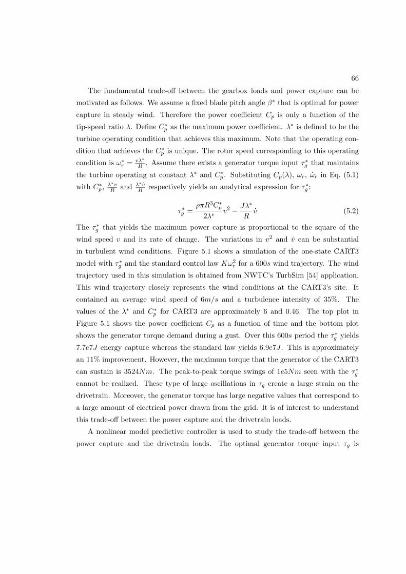
66

The fundamental trade-off between the gearbox loads and power capture can be

motivated as follows. We assume a fixed blade pitch angle β∗ that is optimal for power

capture in steady wind. Therefore the power coefficient Cp is only a function of the

tip-speed ratio λ. Define C∗p as the maximum power coefficient. λ∗ is defined to be the

turbine operating condition that achieves this maximum. Note that the operating con-

dition that achieves the C∗p is unique. The rotor speed corresponding to this operating

condition is ω∗r = vλ∗

R . Assume there exists a generator torque input τ∗g that maintains

the turbine operating at constant λ∗ and C∗p . Substituting Cp(λ), ωr, ωr in Eq. (5.1)

with C∗p ,

λ∗vR and λ∗v

R respectively yields an analytical expression for τ∗g :

τ∗g =ρπR3C∗

p

2λ∗v2 − Jλ∗

Rv (5.2)

The τ∗g that yields the maximum power capture is proportional to the square of the

wind speed v and its rate of change. The variations in v2 and v can be substantial

in turbulent wind conditions. Figure 5.1 shows a simulation of the one-state CART3

model with τ∗g and the standard control law Kω2r for a 600s wind trajectory. The wind

trajectory used in this simulation is obtained from NWTC’s TurbSim [54] application.

This wind trajectory closely represents the wind conditions at the CART3’s site. It

contained an average wind speed of 6m/s and a turbulence intensity of 35%. The

values of the λ∗ and C∗p for CART3 are approximately 6 and 0.46. The top plot in

Figure 5.1 shows the power coefficient Cp as a function of time and the bottom plot

shows the generator torque demand during a gust. Over this 600s period the τ∗g yields

7.7e7J energy capture whereas the standard law yields 6.9e7J . This is approximately

an 11% improvement. However, the maximum torque that the generator of the CART3

can sustain is 3524Nm. The peak-to-peak torque swings of 1e5Nm seen with the τ∗g

cannot be realized. These type of large oscillations in τg create a large strain on the

drivetrain. Moreover, the generator torque has large negative values that correspond to

a large amount of electrical power drawn from the grid. It is of interest to understand

this trade-off between the power capture and the drivetrain loads.

A nonlinear model predictive controller is used to study the trade-off between the

power capture and the drivetrain loads. The optimal generator torque input τg is

67

58 58.5 59 59.5 60 60.5 61 61.5 620.35

0.4

0.45

0.5

Time [s]

Cp

[unit

less

]

58 58.5 59 59.5 60 60.5 61 61.5 62

2400

2600

2800

3000

Time [s]

Kω

2 rG

enTorq

[Nm

]

Kω2

rLaw

τ∗

g

58 58.5 59 59.5 60 60.5 61 61.5 62

−1

0

1

x 105

Time [s]

τ∗ g

Gen

Torq

[Nm

]

Figure 5.1: Control of the CART3 for the maximum power capture

68

calculated at each time step by solving the following optimal control problem:

minimizeτg(t)∈[0,T ]

∫ T

0τ2g (t)− αv3(t)Cp(λ(t)) dt (5.3)

subject to: Equation (5.1)

ωr(0) = ωr0

The τ2g term in the cost function corresponds to minimizing the actuator usage. This

leads to a smaller gearbox damage. The −v3Cp(λ) term represents maximizing the

power capture on rotor. The coefficient α is the weight on the power capture. It is

assumed that v(t) in t ∈ [0, T ) is supplied by an advanced wind preview sensor such

as a LIDAR. In other words, studying this optimization problem for a terminal time

T corresponds to the use of T seconds of wind preview information for control. The

current rotor speed ωr0 is also available to the controller. The τg(t) that yields the

optimal trade-off between these weighted objectives is being calculated. The control

input τg(0) is implemented. The optimization problem is solved again at the next time

step with the new wind and rotor speed measurements. The system is started at the

ωr0 that yields the optimal power coefficient C∗p for v(0). We analyze this problem for

a single, long (600s) realization of the random process v(t). This long realization helps

capture the statistical properties of the v(t). However, more realistic and statistically

meaningful results require solving this problem with many realizations of v(t).

The optimization problem in Eq. (5.3) is a nonlinear optimal control problem with

a fixed terminal time. Denote L(ωr(t), τg(t), t) = τ2g (t) − αv3(t)Cp(λ(t)). The turbine

dynamics in Eq. (5.1) are denoted as ωr = f(ωr(t), τg(t), v(t)). The three necessary

optimality conditions for the optimal τg in Eq. (5.3) are given by [84]:

ωr = f(ωr(t), τg(t), v(t))

ξ = −(∂f

∂ωr

)T

ξ −(∂L

∂ωr

)T

0 =

(∂f

∂τg

)T

ξ +

(∂L

∂τg

)T

(5.4)

with boundary conditions ωr(0) = λ∗v(0)/R and ξ(T ) = 0. ξ(t) is the Lagrange mul-

tiplier function. These equations are known as the Euler-Lagrange equations in the

calculus of variations [84]. This is a two-point boundary-value problem. The partial

69

derivatives in Eq. (5.4) correspond to the following expressions for the turbine control

problem defined in Eq. (5.3):

∂f

∂ωr= −ρπR

2v3Cp(λ)

2Jω2r

+ρπR3v2

2Jωr

dCp(λ)

dλ

∂L

∂ωr= −αRv2dCp(λ)

dλ

∂f

∂τg=

1

J

∂L

∂τg= 2τg

(5.5)

This problem is solved numerically to obtain the optimal control input τg over the

time horizon of t ∈ [0, T ). This solution is obtained as follows. The variables in

Eq. (5.4) (ωr, τg, ξ) are discretized in time with sample time of Ts. The derivative

terms on the left-hand side of the Eq. (5.4) are approximated via forward-differences,

i.e. ωr(0) ≈ (ωr(Ts)− ωr(0))/Ts. The three equations in Eq. (5.4) are converted to the

following nonlinear equations:

M1

ωr(0)

ωr(Ts)

ωr(2Ts)

ωr(3Ts)...

ωr(T )

=

f(ωr(0), τg(0), v(0))

f(ωr(Ts), τg(Ts), v(Ts))......

f(ωr(T − Ts), τg(T − Ts), v(T − Ts))

(5.6)

M1

ξ(0)

ξ(Ts)

ξ(2Ts)...

ξ(T − Ts)

ξ(T )

= −

∂f∂ωr

∣∣t=0

ξ(0)∂f∂ωr

∣∣t=Ts

ξ(Ts)......

∂f∂ωr

∣∣t=T−Ts

ξ(T − Ts)

−

∂L∂ωr

∣∣t=0

∂L∂ωr

∣∣t=Ts......

∂L∂ωr

∣∣t=T−Ts

(5.7)

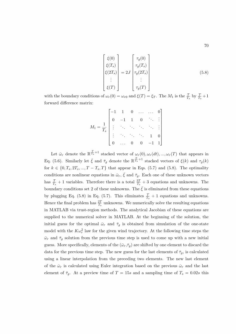
70

ξ(0)

ξ(Ts)

ξ(2Ts)...

ξ(T )

= 2J

τg(0)

τg(Ts)

τg(2Ts)...

τg(T )

(5.8)

with the boundary conditions of ωr(0) = ωr0 and ξ(T ) = ξT . TheM1 is theTTs

by TTs

+1

forward difference matrix:

M1 =1

Ts

−1 1 0 . . . . . . 0

0 −1 1 0. . .

......

. . .. . .

. . .. . .

......

. . .. . .

. . . 1 0

0 . . . 0 0 −1 1

Let ωr denote the R

TTs

+1 stacked vector of ωr(0), ωr(dt), ..., ωr(T ) that appears in

Eq. (5.6). Similarly let ξ and τg denote the RTTs

+1 stacked vectors of ξ(k) and τg(k)

for k ∈ {0, Ts, 2Ts, ..., T − Ts, T} that appear in Eqs. (5.7) and (5.8). The optimality

conditions are nonlinear equations in ωr, ξ and τg. Each one of these unknown vectors

has TTs

+ 1 variables. Therefore there is a total 3TTs

+ 3 equations and unknowns. The

boundary conditions set 2 of these unknowns. The ξ is eliminated from these equations

by plugging Eq. (5.8) in Eq. (5.7). This eliminates TTs

+ 1 equations and unknowns.

Hence the final problem has 2TTs

unknowns. We numerically solve the resulting equations

in MATLAB via trust-region methods. The analytical Jacobian of these equations are

supplied to the numerical solver in MATLAB. At the beginning of the solution, the

initial guess for the optimal ωr and τg is obtained from simulation of the one-state

model with the Kω2r law for the given wind trajectory. At the following time steps the

ωr and τg solution from the previous time step is used to come up with a new initial

guess. More specifically, elements of the (ωr,τg) are shifted by one element to discard the

data for the previous time step. The new guess for the last elements of τg, is calculated

using a linear interpolation from the preceding two elements. The new last element

of the ωr is calculated using Euler integration based on the previous ωr and the last

element of τg. At a preview time of T = 15s and a sampling time of Ts = 0.02s this

71

problem contains 2T/Ts = 1500 variables. Solution of one such optimization step takes

less than 0.1s on a typical desktop computer.

5.3.2 Power Capture versus Drivetrain Loads Trade-off

First we study the impact of the preview time on the optimal performance. A wind

trajectory that represent the turbulence conditions at the CART3 site is generated with

NWTC’s TurbSim code. This trajectory is generated at an average wind speed of 6m/s

and has a turbulence intensity of 35%. T = 15, 30 and 600s of preview times are

investigated. Current preview wind sensors can typically supply wind information up

to 200m distance from turbines. The rated wind-speed of CART3 is 12.5m/s. Therefore

200m preview corresponds to 16s and is sufficient for Region 2 control. The 30s case

investigates the benefits of extra preview. The 600s preview case represents the limiting

case where the full wind trajectory is available to the controller.

The optimization problem in Eq. (5.3) is solved in model predictive control style

over a simulation window of 600s. These simulations are run with different weights on

energy capture (α in Eq. (5.3)) to capture the optimal trade-off between the power cap-

ture and gearbox load reduction objectives. These performance metrics are normalized

with respect to their respective values obtained with the Kω2r law for the same wind

trajectory. Figure 5.2 presents the optimal performance trade-off with different preview

times. It is seen that the 15s preview is mostly sufficient for the optimal control action.

However, it should be noted that larger turbines than the CART3 may require longer

preview times. This is because it is harder to make the larger rotor inertia respond to

large wind gusts. In the case of CART3, T = 30s preview yields a limited performance

improvement over the 15s preview. This performance is almost optimal and the perfor-

mance difference with the limiting 600s preview case is negligible. It is also seen that a

large performance improvement over the standard law can be obtained with the use of

preview. A notable 6% improvement in power capture can be obtained while retaining

similar gearbox loads. Similarly a 30% load reduction can be obtained while achieving

a similar power capture to the Kω2r law. The limiting case for the maximum energy

capture is an 11% improvement over the Kω2r . This is calculated from the analytical

formula given in Eq. (5.2). The corresponding normalized actuator usage, the ratio of

||τg(t)||2 for the maximum power capture case and the Kω2r law, is approximately 25.

72

0.7 0.8 0.9 1 1.1 1.20.98

0.99

1

1.01

1.02

1.03

1.04

1.05

1.06

1.07

1.08

Normalized Actuator Usage

Norm

alize

dE

ner

gy

Captu

re

Pareto Optimal Performance - 35% Turbulence at NWTC

15s Preview

30s Preview

600s Preview

Kω2

rLaw

Figure 5.2: Pareto optimal performance trade-off with different preview times

Figure 5.3 shows the time-domain behavior of the standard control law Kω2r and

the model predictive controller with α = 1.1e5. This model predictive controller yields

the same gearbox loads with the Kω2r law and captures 6% more energy over the 600s

wind trajectory. Figure 5.3 compares the power captured by the rotor, the tip speed

ratio and the generator torque. The wind trajectory used in this problem is presented

in the bottom plot. The optimal tip-speed ratio λ∗ = 6 for CART3 is denoted with the

red-dashed line in the tip-speed ratio plot.

It is possible to gain some simple insight into controller behavior by analyzing the

time-domain results in Figure 5.3. The MPC with preview is able to improve power

capture without much increase in generator torque. This relies on two factors. First, it

is operating closer to λ∗ = 6 when the wind speed is highest. This is crucial for power

capture. Second, the power coefficient Cp(λ) drops more sharply for values λ < λ∗ than

λ ≥ λ∗. This can be seen in Figure 5.4 that presents the Cp − λ curve for the CART3.

Wind gusts can lead to sharp drops in λ below λ∗. The preview MPC controller avoids

this situation to capture more power during gusts. The mean value of the λ for the Kω2r

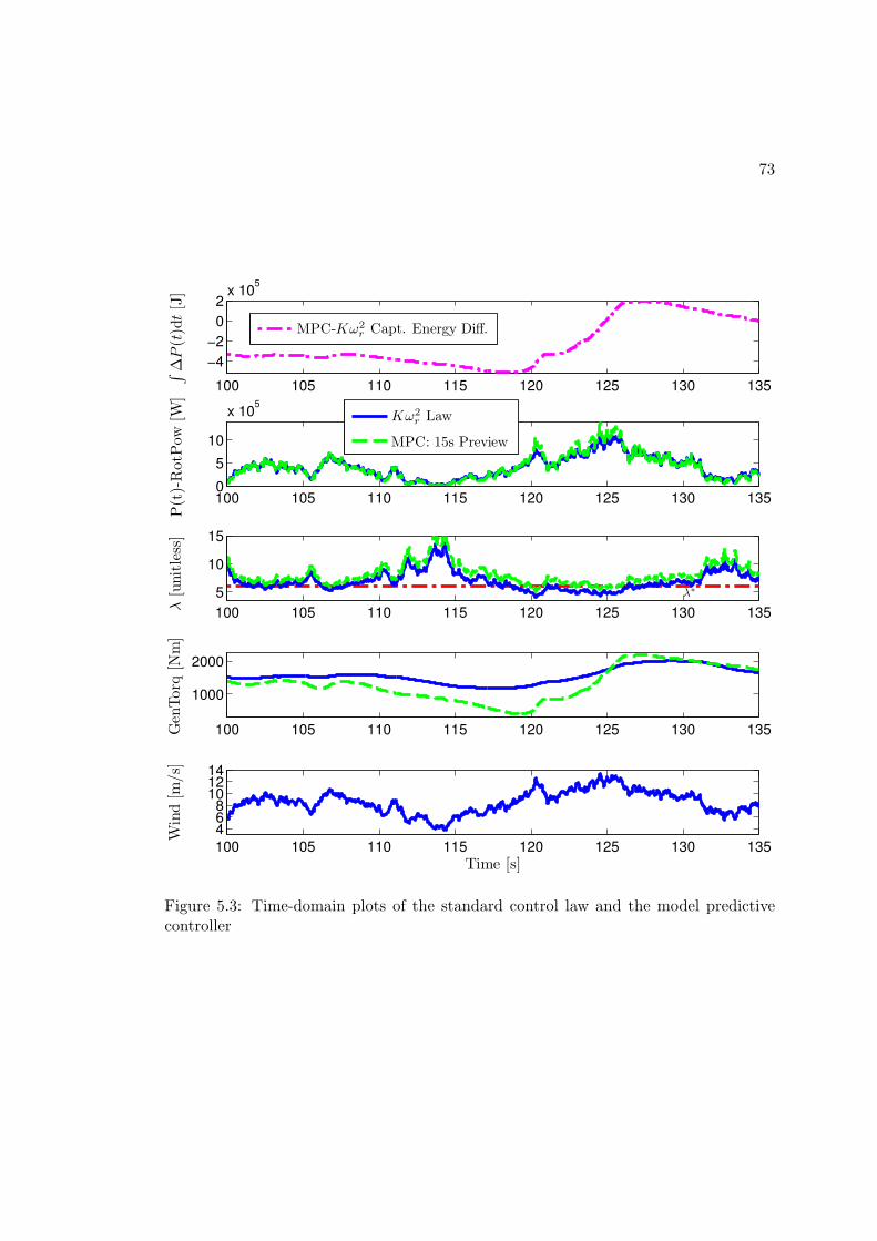
73

100 105 110 115 120 125 130 135

−4

−2

0

2x 10

5

∫∆

P(t

)dt

[J]

MPC-Kω2

rCapt. Energy Diff.

100 105 110 115 120 125 130 1350

5

10

x 105

P(t

)-R

otP

ow[W

]

100 105 110 115 120 125 130 135

5

10

15

λ[u

nit

less

]

λ∗

Kω2

rLaw

MPC: 15s Preview

100 105 110 115 120 125 130 135

1000

2000

Gen

Torq

[Nm

]

100 105 110 115 120 125 130 135

468

101214

Time [s]

Win

d[m

/s]

Figure 5.3: Time-domain plots of the standard control law and the model predictivecontroller

74

3 4 5 6 7 8 9 100.1

0.2

0.3

0.4

Tip Speed Ratio λ

Pow

erC

offi

cien

tC

p(λ

)

Cp(λ) versus λ for the CART3

Figure 5.4: Cp versus λ data for the CART3

and 15s preview MPC are 7.5 and 8.3 respectively. The standard deviations are 3.5 and

2.9, respectively. The preview MPC is sacrificing a small amount of power capture by

operating at larger λ > λ∗. This is especially true during lower wind speeds when the

power capture is less important. The top plot in Figure 5.3 has a slight downward slope

up until t ≈ 118s showing that the MPC is capturing less power. The benefit of this

reduced power is the reduced generator torque. Before the onset of the gusts the rotor

is accelerated such that the λ drops to the λ∗ when the gust hits. This behavior can

be seen at ≈ 120s and ≈ 125s in Figure 5.3. The gain in power capture during gusts

is much larger than the power sacrificed in lower wind speeds. The energy capture

difference between the preview MPC and Kω2r becomes positive rapidly in the top plot

in Figure 5.3. This shows that the MPC is capturing significantly more power during

the highest wind speeds by operating near λ∗. On the other hand, the Kω2r law drops

below the λ∗ value at the highest wind speeds and captures less power.

The second problem investigated is the effect of the turbulence level on the optimal

performance. Three wind trajectories that have an average wind speed of 6 (m/s) and

turbulence intensities of 35%, 22%, and 14% are considered. The 35% turbulent wind

case corresponds to the wind conditions at the CART3 site. A realistic preview time of

T = 15s is considered. The model predictive controller defined in Eq. (5.3) is simulated

over 600s simulation windows. The normalized performance metrics are calculated for

75

each wind trajectory. These results are presented in Figure 5.5. There are three key

observations in Figure 5.5. First, the distance between the Pareto optimal front and

the Kω2r law increases with increasing turbulence intensity. Second, simultaneous large

improvements in power capture and reductions in gearbox loads can be obtained with

use of preview. Third, sustaining larger drivetrain damage than the Kω2r law in low-

turbulent wind conditions yields limited power capture improvements. However, there

is an important trade-off between the extra power capture and the loads with larger

wind fluctuations. Whether a control method that yields higher power with higher

loads is desirable depends on the extra cost incurred by the extra drivetrain damage.

Development of cost models for turbine structures that relate the sustained damage to

an economic cost is an open area of research.

0.7 0.8 0.9 1 1.1 1.20.96

0.98

1

1.02

1.04

1.06

1.08

Normalized Actuator Usage

Norm

alizedEnergyCapture

Pareto Optimal Performance for Preview Time: T=15 (s)

Wind Cond. at NWTC, High Turb.(35%)

Medium Turbulence (22%)

Low Turbulence (14%)

Kω2rLaw

Figure 5.5: Pareto optimal performance trade-off with a fixed preview time of 15 (s)

76

5.4 Region 3 Preview Control1

Turbine Region 3 control problem has different objectives and challenges than the Region

2 control problem. Blade pitch is the main control input used in Region 3 control whereas

the generator torque is held constant or set to achieve a constant power. The large

turbine blades encountered in commercial turbines often have restrictive rate limits.

This section aims to understand the fundamental trade-offs between performance, wind

preview time, and blade pitch rate limits in Region 3 control.

The main control objective is to use preview information to reject wind disturbances

subject to blade pitch rate constraints. We study Region 3 rotor speed regulation prob-

lem using two different fidelity models. First, an optimal control problem is formulated

in continuous-time for a simple one-state, linear rigid-body model of a wind turbine.

The exact, analytical solution of this problem provides insight into the fundamental per-

formance limits. Second, H∞ preview controllers are designed for a number of preview

times. These controllers are simulated on a medium-fidelity, nonlinear turbine model

with realistic preview sensor models. The performance versus preview time characteris-

tics of the H∞ controllers are in agreement with the predictions from the lower-fidelity

models. Thus we believe the analytical results obtained with the low-order model can

provide design guidelines for the use of preview information in turbine control.

The remainder of this section is structured as follows: Section 5.4.1 presents the

problem formulation and the analytical results for the simple one-state model of the

turbine. Section 5.4.2 discusses the results with the medium-fidelity nonlinear model of

the turbine and compares these with the analytical results. The challenges associated

with the preview wind measurements are also discussed in Section 5.4.2.

1 In reference to IEEE copyrighted material which is used with permission inthis thesis, the IEEE does not endorse any of the University of Minnesota’s productsor services. Internal or personal use of this material is permitted. If interested inreprinting/republishing IEEE copyrighted material for advertising or promotional pur-poses or for creating new collective works for resale or redistribution, please go tohttp://www.ieee.org/publications standards/publications/rights/rights link.html to learnhow to obtain a License from RightsLink.

77

5.4.1 Analytical Results for One-State Turbine Model

An exact analytical solution to solve the optimal control problem for a first-order system

with preview information was provided in [85]. This section applies a simplified version

of the results in [85] for rotor speed tracking in above-rated wind conditions (Region

3). The control objective is to minimize the peak tracking error. The L∞ (peak)

norm is used to measure the tracking error for two reasons. First, minimizing the

peak rotor speed error is crucial to avoiding generator over-speed. Second, variations in

rotor speed are correlated to structural loads on the turbine. Hence reducing variations

in rotor speed typically leads to reduced peak blade, tower and gearbox loads. Peak

loads encountered under extreme wind conditions are a driving design factor for large,

commercial wind turbines that contain highly flexible structures.

The wind turbine considered for the analysis is the three-bladed Controls Advanced

Research Turbine (CART3) located at the National Wind Technology Center (NWTC).

The CART3 is chosen for this study because it has been used extensively in the lit-

erature. This provides the opportunity to understand performance trends observed in

previous work on preview control for wind turbines [31] and [33] in the context of the

analytical results provided in this paper.

Problem Formulation

The one-state linear turbine model used for the control problem formulation can be

obtained either from FAST or the one-state nonlinear model described in Section 3.3

and 5.3.1. For the sake of a simple description we assume that this linear model is

obtained from the latter option. Eq. (3.3) has one state (ωr), two control inputs (τg and

β) and one exogenous disturbance (v). Equation (3.3) can be numerically linearized at

a trim condition (ωr, τg, β, v) to obtain a one-state model of the form:

δωr(t) = a δωr(t) + b δβ(t) + c δv(t) (5.9)

Here the ωr is the rotor speed, β is the pitch angle and v is the wind speed. δ denotes

the deviations from these variables’ trim values. The constant coefficients a, b and c

in this linear model correspond to the damping, control gain, and disturbance gain,

respectively. In Region 3 the trim condition ωr is the rated rotor speed and hence

78

δωr(t) is the rotor speed tracking error. The control objective is to regulate δωr(t) to

zero. The disturbance is “matched” in Equation (5.9) and hence it can be perfectly

canceled by setting δβ(t) = − cδv(t)b . However, perfect cancellation is not possible if

the actuator is subject to rate constraints and the wind speed is rapidly changing. An

advanced sensor, e.g. LIDAR, can be used to generate a preview measurement of the

wind disturbance, i.e. a measurement of δv(τ) for τ > t. This preview measurement can

be used to partially overcome the disturbance rejection limitations imposed by actuator

rate constraints.

Assume the controller has access to T seconds of preview wind information. The

essence of the performance vs. preview trade-off is captured by the following control

optimization problem:

p(T ) := minβ∈C[−T,∞)

||δωr ||∞

subject to: Equation (5.9)

|β(t)| ≤ r

δωr(−T ) = 0, δβ(−T ) = 0

δvT (t) =

{0 if t < 0

v∗ if t ≥ 0

(5.10)

where C[−T,∞) is the vector space of continuous functions defined on the interval

[−T,∞). The infinity-norm for the continuous signal δωr is defined as

||δωr ||∞ = supt∈[−T,∞)

|δωr(t)|

In words, the turbine is initialized at the equilibrium δωr(−T ) = 0 and is disturbed by

a wind gust of magnitude v∗ at time t = 0. The objective is to design the optimal

pitch input that minimizes the peak deviation in δωr . Here the pitch rate constraint

is written as |β| < r without the symbol δ since the trim pitch rate ˙β is zero. δβ is

rate constrained and hence the wind gust cannot be perfectly canceled. The control

problem formulation allows δβ to anticipate the disturbance, i.e. the blades can begin

moving at t = −T to cancel the step gust at t = 0. This models a situation in which

the controller has a measurement of the disturbance with T seconds of preview. p(T )

denotes the optimal performance as a function of the preview time T . The rest of the

presentation assumes, without loss of generality, that v∗ ≥ 0.

79

The step wind gusts used in this formulation do not fully capture the effects of

turbulent wind conditions. However, the frequency spectra of many common turbulence

models [54] exhibit a roll-off characteristic similar to of a step gust. Hence step wind

gusts can provide a useful approximation to the turbine performance under turbulence.

The frequency spectrum of the turbulent wind conditions generated for CART3 is

shown in Figure 5.6 (blue solid line). TurbSim [54], developed at NWTC, was used to

generate the turbulent wind data. The parameters for generating the turbulent wind

data are taken from the work by Laks, et al. [33] and are listed in the Table 5.4.1. These

wind conditions are considered to be realistic for the NWTC site where the CART3 is

located. The average wind speed of 18m/s was chosen to ensure constant Region 3

operation. The wind conditions generated by TurbSim include spatial and temporal

variations. Only the frequency spectrum of the hub-height average wind minus the trim

wind speed is shown. The green dash-dotted line in Figure 5.6 is the spectrum of a

2.5m/s step wind gust. The spectrum of the step gust is a good approximation for the

turbulent spectrum over a wide frequency band of 0.01 to 25rad/s. The red dashed

curve in Figure 5.6 is the H∞ design weight used to describe the expected spectrum of

the disturbances. This curve and weight will be discussed further in the next section.

10−2

10−1

100

101

−30

−20

−10

0

10

20

30

40

50

Frequency (rad/s)

Magnitude

(dB

)

TurbSim Wind Data

H∞

Design Weight

Step Wind Gust

Figure 5.6: Frequency spectrum of the hub-height average speed of the turbulent windconditions

The CART3 model [59] is trimmed at v = 18m/s for Region 3 linearization. This

80

Parameter Value

Mean Wind Speed 18 m/s

Vertical Wind Shear (α0) 0.110

Vertical Stability (RiTL) −0.18

Mean Friction Velocity (U∗D) 0.682 m/s

Table 5.1: Atmospheric parameters used in TurbSim for generating turbulent wind data

is approximately the mean of the rated and cut-out wind speed specifications for this

turbine. The rated rotor speed, generator torque and corresponding trim pitch angles

are ω = 3.881rad/s, τg = 152130Nm, and β = 16.52deg. The resulting numerical

values of a, b and c are −0.27711s , −0.0527 1

deg·s2 and 0.0731 1m·s . A step wind gust of

v∗ = 2.5m/s on top of the 18m/s steady wind was used for the problem formulation in

Equation (5.10). This amplitude was obtained from fitting the turbulent wind spectrum

used for CART3 simulations with of a step gust as shown in Figure 5.6. The only

remaining parameter in the optimal control problem (Equation (5.10)) is the pitch rate

limit r. The CART3 pitch actuators have rate limits of 18deg/s. The design value of

the actuator rate limit is conservatively chosen as r = 6deg/s for this analysis. This

conservative choice is made because the controllers designed in this section are also

tested in extreme wind conditions in Section 5.5. A controller designed to yield 6deg/s

peak pitch rate for step and turbulent wind conditions can use higher pitch rates in

extreme wind conditions. These conservative controllers avoid pitch rate saturations

that can destabilize the closed loop system.

The remainder of this section provides the optimal pitch control as a function of the

preview time. Additional details, including proofs of optimality, can be found in [85].

The optimal solution consists of four cases: zero, small, medium, and large preview

times. The characterizations of these four cases depends on a fundamental preview

time defined as T ∗ := cv∗

r|b| . In addition, the optimal solution depends on the non-

dimensional decay rate α := aT ∗. For the CART3 linearization data the constants are

T ∗ = 0.577s and α = −0.160. The results are presented for the approximation that

α = 0 (equivalently a = 0). This introduces less than 1% error because α ≪ 1 for the

CART3 data. More importantly, this approximation leads to simpler analytical formulas

that can be used to gain insight into the preview control problem. This approximation

arises because a utility-scale wind turbine has a large rotor inertia. The large inertia

81

translates into a small decay rate a relative to the fundamental time scale T ∗ that arises

in the preview control problem, i.e. aT ∗ ≪ 1. The exact amount of error introduced by

this approximation can be obtained by comparing the full solution presented in [85] to

the simplified results presented here.

No Preview: T = 0

If there is no preview (T = 0) then the optimal response is to ramp the blades at their

maximum rate β = r until δβ cancels the wind gust. It takes T ∗ := cv∗

r|b| seconds to pitch

the blades δβ from 0 to cv∗

|b| . This optimal input can be written as:

δβ0(t) =

{r(t+ T ) if − T ≤ t < T ∗ − Tcv∗

|b| if t ≥ T ∗ − T(5.11)

Integration of the system dynamics (Equation (5.9)) with a = 0 yields the trajectory:

δω0(t) =

{cv∗(t+ T )− |b|r(t+T )2

2 if − T ≤ t < T ∗ − T(cv∗)2

2r|b| if t ≥ T ∗ − T(5.12)

Therefore the minimal peak rotor speed tracking error (Equation (5.10)) with no preview

is given by p(0) = (cv∗)2

2r|b| .

Small Preview: T ≤(√

2− 1)T ∗

For “small” preview times, the optimal pitch action is still given by δβ0(t) in Equa-

tion (5.11). Specifically, δβ0(t) is optimal for preview times that satisfy T ≤(√

2− 1)T ∗.

Figure 5.7 shows the response of the turbine rotor with the optimal input δβ0(t) for three

different “small” preview times. The wind gust occurs at t = 0 for each response. The

controller starts acting when the wind gust information enters the system at t = −T .In other words, the controller has exactly T seconds to act before the gust. The solid

line in this figure is the response δω0(t) for no preview (Equation (5.12)). For the

CART3 data, T ∗ = 0.577s and the minimal peak rotor speed error with no preview

is p(0) = 0.0527rad/s. The dashed and dash-dotted lines are the optimal responses

for T = 0.1s and T = 0.23s. All three trajectories achieve their peak magnitude at

t = T ∗ − T and have δωr(t) = 0 for t ≥ T ∗ − T .

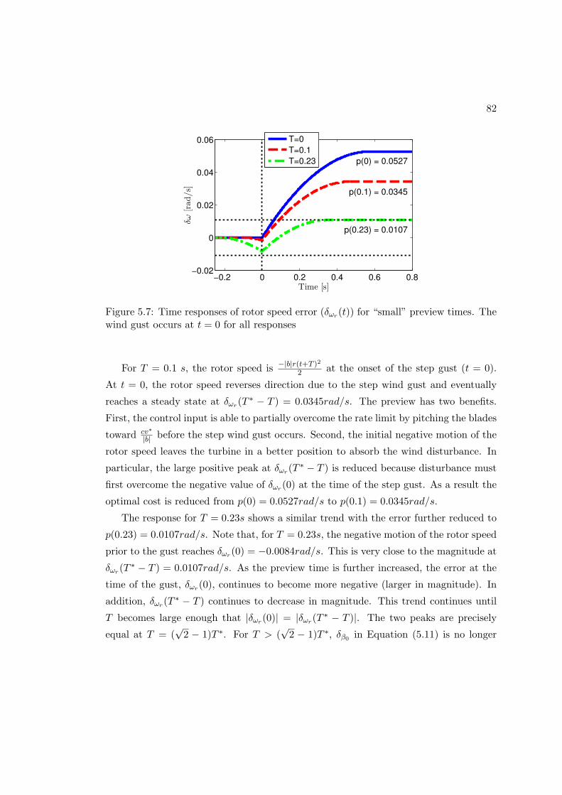
82

−0.2 0 0.2 0.4 0.6 0.8−0.02

0

0.02

0.04

0.06

Time [s]

δω

[rad/s]

p(0) = 0.0527

p(0.1) = 0.0345

p(0.23) = 0.0107

T=0

T=0.1

T=0.23

Figure 5.7: Time responses of rotor speed error (δωr(t)) for “small” preview times. Thewind gust occurs at t = 0 for all responses

For T = 0.1 s, the rotor speed is −|b|r(t+T )2

2 at the onset of the step gust (t = 0).

At t = 0, the rotor speed reverses direction due to the step wind gust and eventually

reaches a steady state at δωr(T∗ − T ) = 0.0345rad/s. The preview has two benefits.

First, the control input is able to partially overcome the rate limit by pitching the blades

toward cv∗

|b| before the step wind gust occurs. Second, the initial negative motion of the

rotor speed leaves the turbine in a better position to absorb the wind disturbance. In

particular, the large positive peak at δωr(T∗ − T ) is reduced because disturbance must

first overcome the negative value of δωr(0) at the time of the step gust. As a result the

optimal cost is reduced from p(0) = 0.0527rad/s to p(0.1) = 0.0345rad/s.

The response for T = 0.23s shows a similar trend with the error further reduced to

p(0.23) = 0.0107rad/s. Note that, for T = 0.23s, the negative motion of the rotor speed

prior to the gust reaches δωr(0) = −0.0084rad/s. This is very close to the magnitude at

δωr(T∗ − T ) = 0.0107rad/s. As the preview time is further increased, the error at the

time of the gust, δωr(0), continues to become more negative (larger in magnitude). In

addition, δωr(T∗ − T ) continues to decrease in magnitude. This trend continues until

T becomes large enough that |δωr(0)| = |δωr(T∗ − T )|. The two peaks are precisely

equal at T = (√2 − 1)T ∗. For T > (

√2 − 1)T ∗, δβ0 in Equation (5.11) is no longer

83

optimal because the blade pitch before the wind gust creates a negative peak at δωr(0)

that dominates the cost. In other words, the control action before the gust specified in

Equation (5.11) does more harm than good.

Moderate Preview:(√

2− 1)T ∗ < T ≤ T ∗

For “moderate” preview times (√2− 1)T ∗ < T ≤ T ∗, the optimal pitch action is of the

form:

δβT(t) =

−r(t+ T ) if − T ≤ t < t1 − T

+r(t+ T − 2t1) if t1 − T ≤ t < 2t1 + T ∗ − Tcv∗

|b| if t ≥ 2t1 + T ∗ − T

(5.13)

where t1 := T 2+2TT ∗−T ∗2

4(T+T ∗) . The subscript in δβTdenotes that the optimal pitch action

depends on T through the parameter t1. For t ≤ t1 − T the optimal input δβTramps

the blades at maximum rate in the wrong direction, i.e. away from the value cv∗

|b|

required to cancel the step wind gust. Then it ramps the blades at maximum rate in

the other direction until it reaches cv∗

|b| . As noted above, the optimal cost for preview time

T = (√2 − 1)T ∗ becomes constrained by the negative peak at δωr(0). The magnitude

of δωr(0) is reduced by ramping the blades initially in the wrong direction. The initial

pitching in the wrong direction allows the system to be closer to the final pitch angle

at the time of gust (t = 0) without causing a larger rotor speed error.

Figure 5.8 shows the rotor speed response and optimal input δβT(t) for three different

“moderate” preview times. The solid, dashed, and dash-dotted lines are the responses

for T = 0.3s, 0.4s, and T ∗ = 0.577s. All three trajectories have δωr(t) = 0 for t ≥2t1 + T ∗ − T . For each preview time the state trajectory δωr(t) achieves the peak

magnitude p(T ) at both t = 0 and t = 2t1 + T ∗ − T . In other words, the value

of t1 is chosen to balance both the negative peak at δωr(0) and the positive peak at

δωr(2t1 + T ∗ − T ).

For each trajectory the optimal control δβTis negative for t < 2t1 − T . This causes

δωr(t) to initially move in the positive direction and achieve a local maximum at δωr(2t1−T ). As the preview time T increases, δωr(2t1 − T ) becomes more positive while the

magnitudes of δωr(0) and δωr(2t1 + T ∗ − T ) are both reduced. When T = T ∗ the first

positive peak at t = 2t1−T satisfies |δωr(2t1−T )| = |δωr(0)| = |δωr(2t1+T ∗−T )|. For

84

−0.6 −0.4 −0.2 0 0.2 0.4−0.01

0

0.01

Time [s]

δω

[rad/s]

−0.6 −0.4 −0.2 0 0.2 0.4

0

2

4

Time [s]

δβ

[deg

]

T=0.3

T=0.45

T=0.577

Figure 5.8: Time responses of rotor speed error (δωr(t)) and optimal pitch command(δβ(t)) for “moderate” preview times. The wind gust occurs at t = 0 for all responses

T > T ∗, the input δβTin Equation (5.13) is no longer optimal because the magnitude

of δωr(2t1 − T ) dominates the cost. For the given data, T ∗ = 0.577s and hence the

dash-dotted curve in Figure 5.8 represents the optimal response for the limiting case

of “moderate” preview (T = T ∗). The optimal input δβ shown in the bottom subplot

changes from δβ = −r to δβ = +r at t1 − T . The top subplot shows that the optimal

δωr(t) for T = 0.577 s achieves its maximum magnitude at times 2t1 − T , 0, and

2t1 + T ∗ − T .

One issue may arise with “moderate” preview times when the wind speeds are just

above the rated wind speed required for Region 3 operation. The initial blade pitch

action with δβ = −r is limited in this situation since the blades may hit the β lower-

bound of pitch-to-feather turbines. This means the blade pitch angles cannot be lowered

any more to gain rotor speed before the gust. In this case the performance can be

conservatively considered to be bounded by the performance given with “small” preview

times. This is a limited performance loss since “moderate” preview times yield limited

performance improvement as seen in Figure 5.9.

85

Long Preview: T > T ∗

For T > T ∗ one might suspect that p(T ) can be further reduced by pre-pending the

control action δβT∗ (t) with an initial negative ramp of the blades. This might simul-

taneously reduce the magnitudes of δωr(2t1 − T ), δωr(0), and δωr(2t1 + T ∗ − T ) which

constrain the performance for T = T ∗. In actuality, no further improvement can be ob-

tained for T > T ∗, i.e. there is a fundamental bound on the performance improvements

achieved via preview. This fact is formalized in the following theorem:

Theorem 1 p(T ) = p(T ∗) for all T ≥ T ∗ = cv∗

r|b| . The minimal cost is p(T ∗) = (cv∗)2

16r|b|

Proof: Follows from reference [85].

The optimal input for T > T ∗ is not unique but one choice is given by:

δβT(t) =

{0 if t < −T ∗

δβT ∗ (t) if t ≥ −T ∗(5.14)

where δβT∗ is the optimal input given by Equation (5.13) for T = T ∗. This choice wastes

the first T − T ∗ seconds of preview by leaving the input at zero and then executes the

control action δβT∗ once T ∗ seconds of preview remains.

Summary

The solution to the optimal control problem (Equation (5.10)) for a = 0 (no damping

in Eq. (5.9)) is summarized in Table 5.2. Figure 5.9 shows the minimum rotor speed

error versus preview time. T ∗ = cv∗

r|b| is a fundamental preview time beyond which no

additional performance improvements are obtained. The fundamental preview time and

optimal tracking cost p(T ∗) are both inversely related to the rate limit r and control

gain b in Eq. (5.9). T ∗ grows linearly with increasing magnitude of the wind gust v∗

and disturbance gain c while p(T ∗) grows quadratically. In addition, p(0) = (cv∗)2

2r|b| and

p(T ∗) = (cv∗)2

16r|b| . Thus, preview information can, at best, reduce the peak tracking error

by a factor of eight compared to the performance with no preview. Finally, the use of

preview has the largest impact for T ≤ (√2 − 1)T ∗. For these small preview times,

the rotor speed error reduces linearly in T . Only minor improvements in the cost are

obtained for preview times (√2− 1)T ∗ < T ≤ T ∗.

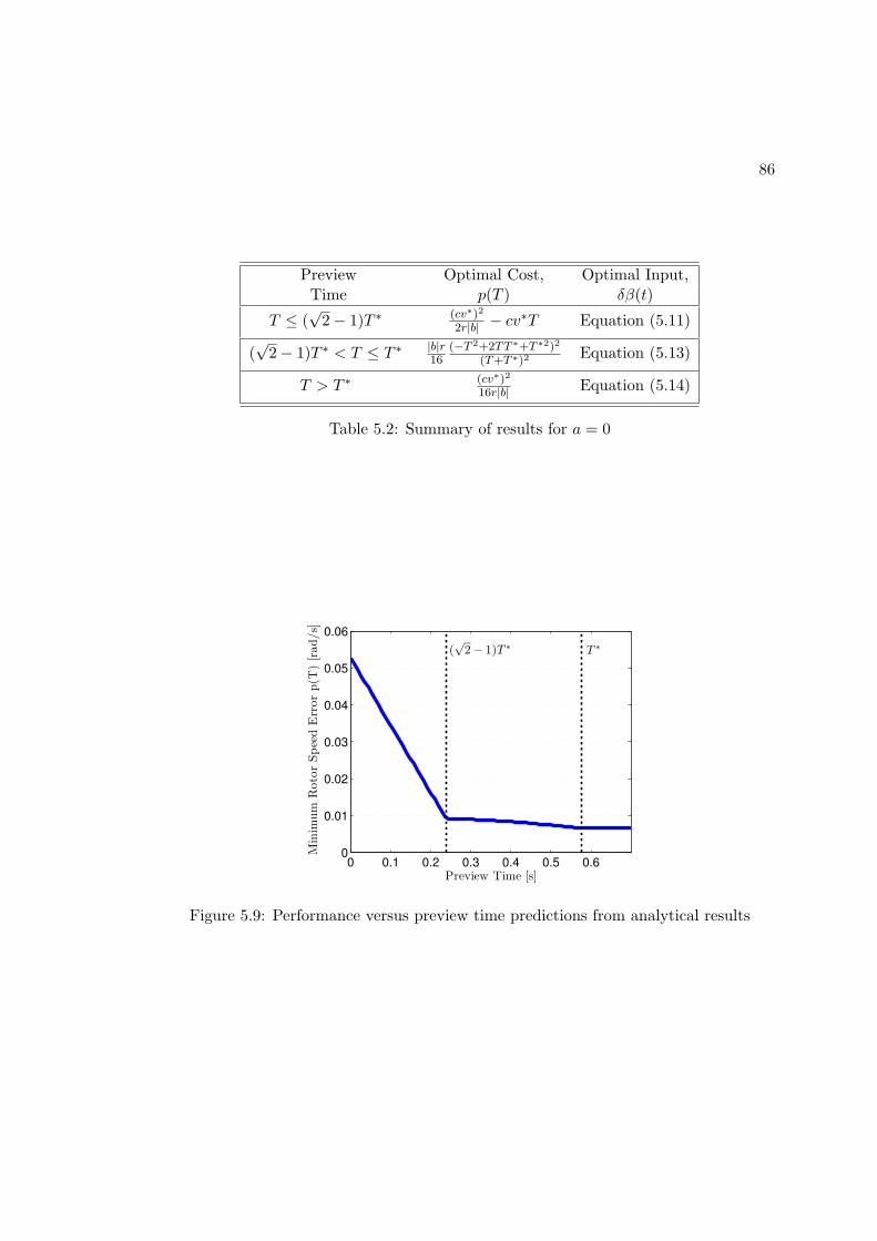
86

Preview Optimal Cost, Optimal Input,Time p(T ) δβ(t)

T ≤ (√2− 1)T ∗ (cv∗)2

2r|b| − cv∗T Equation (5.11)

(√2− 1)T ∗ < T ≤ T ∗ |b|r

16(−T 2+2TT ∗+T ∗2)2

(T+T ∗)2 Equation (5.13)

T > T ∗ (cv∗)2

16r|b| Equation (5.14)

Table 5.2: Summary of results for a = 0

0 0.1 0.2 0.3 0.4 0.5 0.60

0.01

0.02

0.03

0.04

0.05

0.06

Preview Time [s]

(√

2 − 1)T ∗T

∗

Min

imum

Roto

rSpee

dE

rror

p(T

)[rad/s]

Figure 5.9: Performance versus preview time predictions from analytical results

87

Effect of Operating Condition

The results presented in the previous sub-sections are based on a 1-state rigid body

model of the CART3 trimmed at 18 m/s. The parameters a, b and c of this model

change with the mean wind speed. We have obtained linearizations from the rated

wind speed of the CART3, 12.5m/s, up to 24m/s to investigate the effect of operating

conditions on preview time requirements. The b and c parameters from each of these

models are used to calculate the fundamental preview time T ∗. Figure 5.10 shows the T ∗

versus the trim wind speed. The T ∗ = 83s calculated for 12.5m/s trim wind condition is

not plotted. This is because T ∗ decreases rapidly with increasing trim wind speed. Trim

pitch angle difference between 12.5m/s and 12.6m/s is approximately 1.5deg. Blades

with the pitch rate limit 18deg/s can travel 1.5deg in a much shorter time than the

difference in the fundamental preview times between these two trim wind speeds.

The preview time versus trim wind speed trend observed in Figure 5.10 agrees well

with general turbine design considerations. This trend is largely driven by the variations

in the control gain parameter b. Turbine power and torque capture are designed to be

insensitive to pitch angle variations around the optimal pitch angle for power capture

in Region 2. This corresponds to a small b value. This is in order to minimize power

losses due to uncertainties related to calculation of this optimal pitch angle. As the

turbine enters Region 3, the pitch angle is increased to shed some of the power in wind.

To achieve this effect the turbine design favors a higher b value at increasing pitch

angles. For instance, b = −0.0070 and −0.0260 at trim wind speeds equal to 12.6m/s

and 14m/s, respectively. The fundamental preview time T ∗ is inversely related to b.

Hence the increase in control effectiveness b from 12.6m/s to 14m/s corresponds to the

decrease in fundamental preview time.

5.4.2 Validation with H∞ Preview Controllers

This section presents an H∞ preview controller using a design architecture similar to

that used by Laks, et al. [31]. This is a 2-input (rotor speed and wind speed measure-

ments) and 1-output (collective pitch) controller. The performance vs. preview time

is evaluated using the NWTC’s Fatigue, Aerodynamics, Structures, and Turbulence

(FAST) nonlinear simulation code [51]. A detailed LIDAR sensor model is implemented

88

12.6 14 16 18 20 22 24

0.5

1

1.5

2

2.5

3

3.5

Trim Wind Speed [m/s]Fundam

enta

lP

revie

wT

ime,

T∗

[s]

Figure 5.10: Fundamental preview time versus trim wind speed

to capture the challenges associated preview wind sensing. The performance trends

for this medium-fidelity model are compared with the trends predicted by the simple,

rigid-body analysis described in the previous section.

A low order linear model of the CART3 was used for the control design. The low

order, 5 degrees of freedom design model contained modes for generator speed, tower first

fore-aft bending and blade first flapwise bending. This model is based on a linearization

of the FAST model of CART3 at 18m/s hub-height wind speed. The turbine dynamics

depend on rotor position and have a non-steady trim trajectory. Hence linearizations

are performed on a grid of rotor positions and result in linear time-varying (LTV)

models. This LTV model is converted to an LTI model using the multi-blade coordinate

transformation [20,37,63,67,69] followed by averaging of the resulting matrices. Finally,

the turbine model was discretized using a bilinear (Tustin) transformation with a sample

time of Ts = 0.025s. The discretization step was needed for modeling of the wind preview

information. Finally, the first-order pitch actuator models with 30 rad/s bandwidth were

added to the design model. The final design model had 11 states. The continuous time

model without the actuators has the following form before the discretization step:

x =Ax+Bu

y =Cx+Du

89

CollectiveBladePitchCommand

- +

+

?Win

?

InputUncertainty

-Pact

ActuatorModel

Act.PitchRate(δβ)

-PitchAngles (δβ)

6Wact

6

Pitch RatePenalty Wind

?Wwnd

-Delays

1zN

-LTITurbineModel

-∆MBlade

-∆MTower

-∆ωrWperf

---

WeightedPerf.

��

+

+

�

Wnois� Sensor

Noise

6�Controller

Inputs

Figure 5.11: System Interconnection for H∞ Collective Pitch Controller Design

The first two states of this linear system are the tower 1st tower fore-aft bending mode

tip-displacement (m) and rotor position (rad). The next three states correspond to

the collective and cyclic 1st blade flapwise bending mode displacements. States 6-

10 are the derivatives of the first five states. The system inputs are the hub-height

wind disturbance (m/s) and collective blade pitch angles (rad). The outputs are the

collective blade flapwise root bending moment (kN · m), tower base fore-aft bending

moment (kN ·m) and rotor speed (rpm). The state and output matrices have the block

partitioned form:

A =

[0 I5

A21 A22

]

C =[C1 C2

]The system matrices are given by:

A21 =

−34.76 −0.0616 4.709 0.2444 −1.483

−0.7381 −0.0016 2.431 −0.0007 −0.0304

72.79 0.0822 −238.7 −0.697 2.370

6.918 −10.54 −1.269 −186.5 −13.32

−49.13 −8.738 5.088 13.98 −188.5

90

A22 =

−0.1006 −0.0605 0.0049 0.0023 0.0106

−0.0125 −0.0781 0.013 −0.0001 0.0014

−6.375 −19.58 −3.680 0.0264 0.0095

10.74 0.0979 0.0567 −3.518 −7.765

5.404 −0.511 0.0997 7.765 −3.501

B =

0 0

0 0

0 0

0 0

0 0

0.0775 −2.1115

0.0118 1.1015

6.0254 −405.343

−0.0254 29.4093

−0.7780 11.8315

C1 =

192.5 0.389 900 −1.24 9.04

58220 50.81 −211 −153.5 1173

0 0 0 0 0

C2 =

−7.58 −9.18 0.383 −0.0006 −0.099

24.92 −3.42 −0.447 −1.520 −6.969

0 9.55 0 0 0

D =

7.8878 −219.6507

−3.7719 102.9489

0 0

A H∞ preview controller is designed based on this reduced-order, discrete-time LTI

model of the CART3. The control objective is rotor speed tracking as well as tower

91

and blade load reduction at higher (Region 3) wind speeds. The control input is the

collective pitch angle of three blades. The measurement for control is the rotor speed.

In addition, it is assumed that the controller has access to a preview wind measurement

that is the average of three point measurements in space supplied by the LIDARs.

The preview measurements are modeled by augmenting the wind disturbance input of

the design model with N delays. The controller has access to a measurement of the

wind disturbance input to the chain of N delays. As a result, the controller has a

measurement of the wind disturbance with a preview of NTs seconds prior to its impact

on the turbine. The amount of preview available to the H∞ controller is adjusted by

changing the number of delays N .

Signal-weighted H∞ control designs were performed for a variety of preview times N

using the system interconnection shown in Figure 5.11. The block labeled “LTI Turbine

Model” is the discrete-time LTI design model without the actuator dynamics and the N

steps of delay on the wind input. The block Pact contains the pitch actuator model for

CART3. The first output of this model is the actuator pitch rate and the second output

is the pitch angle. The extra pitch rate output was created to penalize blade pitch rates

to normalize control usage across all the designs. The system interconnection contains

weights for performance, input uncertainty, measurement noise, actuator usage, and

wind disturbance. All weights except Wact, which penalizes the pitch command rate,

are independent of the preview time. The weights were initially specified in continuous-

time and then converted to discrete-time using a bilinear (Tustin) transformation with

a sample time of Ts = 0.025s.

The continuous-time transfer functions for each weight are provided in the Table 5.3.

The performance weight is block diagonal Wperf = diag(WBladeM ,WTowerM ,Wωr) with

the individual blocks penalizing flapwise collective blade bending moment, tower fore-

aft bending moment, and rotor speed tracking respectively. The performance penalty

WBladeM emphasizes attenuation of the blade bending moment at middle to high fre-

quencies. This choice is made because the DC and lower frequency components of the

blade bending moments, due to persistent wind disturbances, cannot be attenuated.

The penalty weight on the tower bending WTowerM is chosen to add extra damping

at the tower bending moment frequency. The performance penalty Wωr is chosen to

attenuate low-frequency tracking errors. The input disturbance Win models dynamic

92

uncertainty across all frequencies. The weight Wnois = diag(Wn,ωr ,Wn,wnd) is a 2 × 2

diagonal weight that models noise on the rotor speed and wind speed, respectively. The

rotor speed and wind speed measurement noise weights are chosen as a high pass to

avoid excitation of the high-frequency modes of the turbine. The actuator weight Wact

is used to penalize the blade pitch rates. This penalty acts directly on the pitch rates as

opposed to the pitch command rates. The gain of the constant weight K is chosen as a

function of the wind preview time N . The value of K is tuned through simulations to

obtain a closed-loop peak pitch rate of 6 deg/s for a 2.5 m/s uniform wind gust input

for all H∞ controllers of different preview lengths. This ensures that controllers for all

preview times have roughly the same actuator usage. This normalization is carried out

so that the H∞ controllers have the same peak pitch rate with the analytical solutions

presented in the previous section. Values of gain K versus preview time are provided

in Table 5.4. The second column of this table, denoted as “Delay States (N)”, lists

the number of delay states used in the design interconnection to model preview wind

information.

One design weight of particular importance is the weight on the wind disturbance

Wwnd. This weight represents the frequency spectrum of the operating wind conditions.

This spectrum is important because the preview time required for optimal pitch action

depends on the turbulent wind conditions. For instance slow wind variations with small

magnitude require smaller preview times. Larger magnitude fluctuations observed in

higher turbulence require longer preview times. The weight Wwnd used in this design

is obtained from time-series turbulent wind data generated by TurbSim as described in

the Section 5.4.1. The frequency spectrum of this wind profile, shown in Figure 5.6, is

fit with a first-order transfer function to obtainWwnd. The preview time required by the

H∞ controllers depend on this weight. This is similar to the fact that the fundamental

preview time T ∗ is related to the step wind gust magnitude v∗ used in the analytical

results.

Results with Ideal Measurements

This section presents the results with ideal preview measurements. Note that this

“ideal” measurement case is still impacted by the prediction errors regarding future

rotor position and the Taylor’s frozen turbulence assumption.

93

Weight Transfer Function

Wωr 0.002s+ 50

s+ 0.05

WBladeM 2× 10−7 s+ 50

s+ 0.2

WTowerM 5× 10−7 s+ 50

s+ 5

Win 0.03

Wn,ωr 1.5s+ 0.1

s+ 5

Wn,wnd 15s+ 0.5

s+ 75

Wwnd2.64

s+ 0.12

Wact K(N)

Table 5.3: Weights for H∞ Preview Control Design

Preview Time (s) Delay States (N) Gain K

0 0 3.850

0.10 4 3.250

0.20 8 2.700

0.30 12 2.100

0.40 16 1.500

0.50 20 1.000

0.60 24 0.500

0.70 28 0.035

0.80 32 0.041

≥ 0.80 ≥ 32 0.041

Table 5.4: Values of gain K used in actuator penalty weight Wact

94

The closed-loop response of the nonlinear CART3 system to a 2.5 m/s uniform

wind step disturbance is shown in Figure 5.12 for H∞ controllers with three different

preview lengths. The blue solid, red dashed, and green dash-dot lines are the responses

for the controllers with 0.0s, 0.4s, and 0.8s of preview, respectively. The simulation

results are time shifted such that the step wind gust occurs at t = 0. The controller

with small 0.4s preview starts pitching the blades as soon as information about the

incoming gust in received (t = −0.4s). The control action looks similar to that of the

no-preview controller but time-shifted by 0.4s. This behavior shows close agreement

with the predictions from the analytical results, i.e. similar pitch action for small and

no preview. As the preview time increases further 0.8s, the controller starts pitching

the blades earlier at t = −0.8s. The additional preview enables the controller to achieve

larger pitch angles at the time of the gust (t = 0) than the other controllers. The H∞

controller achieves a much smaller error by having a more negative (larger in magnitude)

error before the gust. The H∞ controllers with preview times larger than 0.8s yield

very similar results to the controller with 0.8s preview and are not plotted. The long

preview time (0.8s) used here is slightly longer than the T ∗ = 0.577s calculated with

the analytical results. The initial pitching toward the fine pitch angle with long preview

times observed with analytical results are not seen here. The analytical result uses the

L∞ (peak) norm to measure performance while the H∞ norm is induced by the L2

(power) norm on signals. We believe the difference in behavior is simply due to this

difference in the objective functions of the optimizations.

Figure 5.13 summarizes the rotor speed tracking performance of the H∞ controllers

on the nonlinear FAST simulations with step and turbulent wind gusts with ideal three

point measurements of the wind field. The blue stars represent H∞ controllers with

step wind gusts. The red circles are the H∞ controllers in turbulent wind conditions.

The green triangles are the analytical solutions based on the one-state rigid body rotor

model of the turbine. All nonlinear simulations with step gusts had peak pitch rates

between 5.95 and 6.05 (deg/s). The nonlinear simulations in turbulent wind had peak

pitch rates between 4.75 and 7 (deg/s). The vertical lines in this plot correspond to the

“small” and “long” preview times predicted by analytical solutions.

There are three key observations in Figure 5.13. First, the peak rotor speed error is

95

−1 0 1 2 3−0.05

0

0.05

0.1

H∞ Controllers on FAST - Step Gust at t = 0

RotS

pE

rr.

δω

r[r

ad/s]

−1 0 1 2 3

18

20

22

Pit

chA

ngle

β[d

eg] No Preview

0.40s Prev.

0.80s Prev.

Figure 5.12: Closed-loop response of the CART3 FAST model to a 2.5 m/s step uniformwind gust. The wind gust occurs at t = 0 for all responses

0 0.1 0.2 0.3 0.4 0.5 0.6 0.7 0.8

0.05

0.1

0.15T ∗(

√2 − 1)T ∗

p∗

Preview Time [s]

||δω

r|| ∞

[rad/s]

Perf. vs. Preview - 2.5m/s Step Wind Gust

H∞

− Turb. Wind

H∞

− Step Gust

Analytical

Figure 5.13: Peak rotor speed error vs. preview time for step and turbulent wind forH∞ controllers on FAST simulations. Ideal three point measurements of the wind fieldis used.

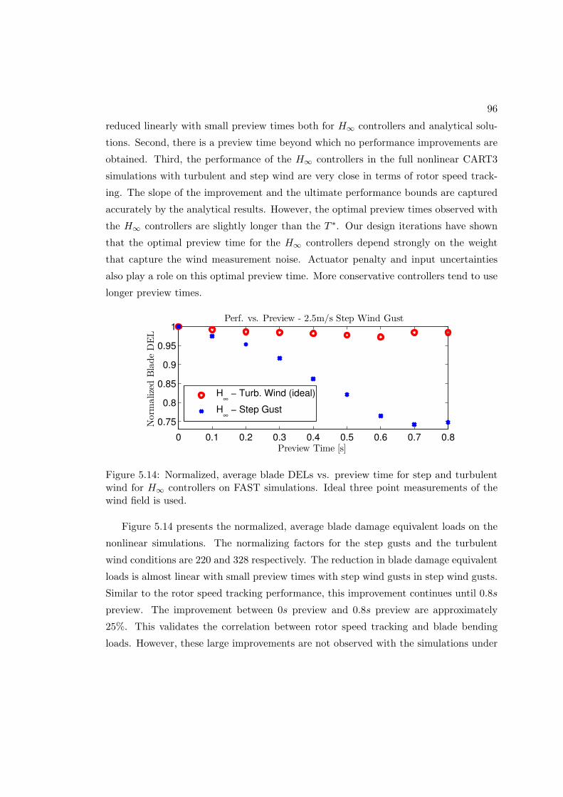
96

reduced linearly with small preview times both for H∞ controllers and analytical solu-

tions. Second, there is a preview time beyond which no performance improvements are

obtained. Third, the performance of the H∞ controllers in the full nonlinear CART3

simulations with turbulent and step wind are very close in terms of rotor speed track-

ing. The slope of the improvement and the ultimate performance bounds are captured

accurately by the analytical results. However, the optimal preview times observed with

the H∞ controllers are slightly longer than the T ∗. Our design iterations have shown

that the optimal preview time for the H∞ controllers depend strongly on the weight

that capture the wind measurement noise. Actuator penalty and input uncertainties

also play a role on this optimal preview time. More conservative controllers tend to use

longer preview times.

0 0.1 0.2 0.3 0.4 0.5 0.6 0.7 0.8

0.75

0.8

0.85

0.9

0.95

1Perf. vs. Preview - 2.5m/s Step Wind Gust

Preview Time [s]

Norm

alize

dB

lade

DE

L

H∞

− Turb. Wind (ideal)

H∞

− Step Gust

Figure 5.14: Normalized, average blade DELs vs. preview time for step and turbulentwind for H∞ controllers on FAST simulations. Ideal three point measurements of thewind field is used.

Figure 5.14 presents the normalized, average blade damage equivalent loads on the

nonlinear simulations. The normalizing factors for the step gusts and the turbulent

wind conditions are 220 and 328 respectively. The reduction in blade damage equivalent

loads is almost linear with small preview times with step wind gusts in step wind gusts.

Similar to the rotor speed tracking performance, this improvement continues until 0.8s

preview. The improvement between 0s preview and 0.8s preview are approximately

25%. This validates the correlation between rotor speed tracking and blade bending

loads. However, these large improvements are not observed with the simulations under

97

turbulent wind. The improvement obtained in this case is approximately 3%. Even

though this performance depends on the design weights, we anticipate this gap to be

due to the strong spatial variation of the wind over turbine blades with realistic full-

field wind trajectories. This renders the use of collective pitch control for blade load

reduction less effective. Individual pitch control with preview wind information may be

used to address this issue.

The tower fore-aft bending moments and the RMS rotor tracking speed errors in step

and turbulent wind conditions in FAST simulations are not shown here. These results

follow the same trend as the peak rotor speed errors shown in Figure 5.13. Almost

linear improvements are observed at low preview times and the improvements stop at

0.8s preview.

The results presented in this section are in agreement with the results in [31] which

present the worst case gains of various H∞ preview controllers designed for the CART3.

The worst-case gain of the controller with 6deg/s pitch rate limit approximately flattens

out at 0.65s of preview. This is a slightly shorter preview time than the one predicted

here. But reference [31] does not use a frequency-based weighting for the wind distur-

bances. The optimal preview time depends on the design weight choice. Results in [31]

also show that there is a fundamental performance limitation imposed by the pitch rate

constraints regardless of the preview time. The worst-case gain versus preview time

plots flatten out at a higher gain for controllers with smaller pitch rate bounds. This

agrees with the results presented in Section 5.4.1 which shows that the optimal cost

with long preview is inversely proportional to the pitch rate bounds.

Results with Realistic LIDAR Measurements

Figure 5.15 compares the performance of the H∞ controllers with ideal measurements

presented in Section 5.4.2 to their performance with realistic preview wind measure-

ments. These results capture the error characteristics of typical continuous wave LI-

DARs but use the Taylor’s frozen turbulence hypothesis. Specifically, wind measurement

errors from spatial range weighting and projection of the horizontal wind onto the laser

beam are incorporated on top of the errors caused by the rotor position prediction. The

results with LIDAR models under 0.3s are not plotted since the large measurement

errors from larger measurement angles from the horizon are extremely detrimental to

98

turbine performance. The key conclusion from Figure 5.15 is that the error character-

istics of the LIDAR sensors may require a longer preview time than the ones observed

with the ideal measurements. The main reason behind this behavior is the large angle

between the LIDAR beam and the horizon when trying to measure wind at the 75%

blade span with small preview. The LIDAR measures the projection of the three di-

mensional wind speed along its beam. The increased angle between the horizon and

the beam reduces the contribution of the horizontal wind speed to the measurement

and increases the contributions of the vertical and side-wise wind speed. Increasing

the preview time allows the LIDAR to obtain measurements at the same blade span

with a smaller angle with the horizon. It is observed that the performance with real-

istic measurement get fairly close to the ideal performance with higher preview times.

It should be noted that using too long preview times can also deteriorate the turbine

performance. At long preview times the range weighting errors and the errors from the

frozen turbulence hypothesis can dominate the measurement errors and be detrimental

to turbine performance.

0 0.1 0.2 0.3 0.4 0.5 0.6 0.7 0.8

0.2

0.4

||δω

r|| ∞

[rad

/s]

Perf. vs. Preview - Turbulent Wind

0 0.1 0.2 0.3 0.4 0.5 0.6 0.7 0.8

350

400

450

500

Avg.

Bla

de

DE

L

Preview Time [s]

H∞

−Turb. Wind (ideal)

H∞

−Turb. Wind (LIDAR)

Figure 5.15: Performance metrics vs. preview time for H∞ controller simulations inturbulent wind and realistic LIDAR sensor models on FAST

99

Summary of Results

In summary, the performance of the advanced preview controllers depend on the pitch

rate limits as well as the aggressiveness of the control design. The analytical formulas

provide a method to predict the performance limits and trends for these controllers

before any detailed control design. The simple steps taken for these predictions can

be summarized as follows. A one-state nonlinear model that captures rigid-body rotor

dynamics is linearized to obtain (a, b, c) parameters. The analytical results presented in

Section 5.4.1 depend on a step wind gust magnitude. This gust magnitude is obtained

from the frequency spectrum of realistic turbulent wind conditions for turbine site. The

second parameter required for the analytical solutions, the peak blade pitch rate, is

obtained from simulation of the H∞ controllers with step wind gusts. It is important

to test the final controllers in medium to high-fidelity simulations with LIDAR sensor

models. It was observed that the error characteristics of these sensors may necessitate

use of longer preview times than the ones predicted by the analytical formulas.

5.5 Preview Control for Extreme Events

In this section we present a framework that can be used to analyze the turbine per-

formance versus preview characteristics for a given arbitrary disturbance signal as a

function of time. This is in contrast to the step wind gust approximation used to derive

our analytical results in Section 5.4.1. The motivation for developing this framework

comes from the extreme operating conditions the turbines can face once a year or once

in fifty years. Turbine structural health must be tested in the field or with simulations

for these extreme conditions [45]. These conditions are described with specific distur-

bance inputs as a function of time in turbine certification guidelines. There is a need for

a method that can be used to analyze the impact of preview on alleviating the effects

of these extreme conditions. We present this framework and demonstrate an example

with a 50-year extreme operating gust as described by the Germanischer Lloyd wind

turbine certification standards [45] on the CART3.

A discretized version of the optimal control problem used for the analytical results

for Region 3 preview control, Eq. (5.10), can be utilized to analyze turbine performance

for specific wind trajectories. The infinite-dimensional optimization in Eq. (5.10) can be

100

converted to a finite-dimensional linear program. This approach offers two key benefits.

First, a specific wind trajectory can be used to analyze the limits of performance.

Second, it is possible to analyze higher order linear models. This allows the introduction

of turbine structural modes and actuator models in the optimization problem.

The approach described here has close ties to the work by Boyd and Barratt [86]

and Dahleh and Diaz-Bobillo [87]. Boyd and Barratt use the Youla parametrization to

formulate wide classes of linear control design problems with time and frequency domain

constraints as convex optimizations. Solution of the convex optimizations can be used

to determine if there exists a controller that satisfies the given design constraints. The

work contained in this paper is influenced by these studies of fundamental performance

limits. Dahleh and Diaz-Bobillo consider the L1 optimal control problem: Find a con-

trol K that minimizes the closed loop induced L∞ (peak) norm from disturbances to

errors. Linear programming (LP) techniques are used to solve for the optimal controller.

We also use L∞ (peak) signal norms and LP techniques. The L∞ norm of the error

signal is minimized for a given disturbance signal rather than for a class of L∞ norm

bounded disturbance signals. This enables analysis of the optimal control action based

on a particular wind trajectory. In addition, we focus on understanding the limits of

performance. No effort has been made to synthesize feedback controllers. Implemen-

tation of the proposed control actions synthesized by LP techniques can be realized in

MPC style but this is not investigated in this thesis.

We envision that the proposed approach can be employed in various ways. First,

given a wind profile it is possible to analyze the optimality of various control designs.

Second, the impact of the preview wind information versus controller performance can

be studied in time-domain. Lastly, linear programming results can be used to develop

insight about controller behavior.

The remainder of the section is structured as follows: Section 5.5.1 formulates an

optimal rotor speed tracking problem with wind preview information as an LP. Sec-

tion 5.5.2 uses this framework to analyze the trade-off between performance versus

preview time characteristics of the NREL’s CART3 [59] for a 50-year gust. This analy-

sis is based on a low-order rotor-inertia model of CART3. We also test the performance

of the H∞ controllers designed in Section 5.4.2 on the nonlinear FAST turbine simu-

lation package. These results are compared with the performance trade-offs computed

101

using the LP framework. Our results show that the H∞ controllers that were designed

without these extreme events in mind result in poor performance. The H∞ controllers

can be modified to better attenuate the effects of this 50-year gust.

5.5.1 Problem Formulation

The control objectives during extreme events are the same with the Region 3 control:

maintaining a constant rotor speed and reducing the structural loads. Therefore the

problem posed here has many similarities with the one presented in Section 5.4.1. In

summary, peak over time rotor speed error minimization is considered. This is important

for avoiding generator over-speed problem during an extreme gust. We rely on the

correlation between the peak structural loads and the peak rotor speed tracking error

for load reduction. It is assumed that a disturbance trajectory as a function of time

is provided. The one-state continuous-time linear model in Section 5.4.1 is replaced

with an n-state discrete-time linear model. These linear models are typically obtained

from medium to high-fidelity, nonlinear turbine models that involve tower and blade

structural modes, models of aeroelastic behavior and turbulent wind profiles. It is

assumed that an LTI approximation is used for the periodic LTV models resulting

from linearization. Some of the common LTI approximation methods are explained in

Section 3.5.2.

The linear turbine model is assumed to have the following form:

x[k + 1] = Ax[k] +Bu[k] +Bdud[k]

e[k] = Cx[k](5.15)

Here A ∈ Rn×n, B ∈ Rn×1, Bd ∈ Rn×1 and C ∈ R1×n. In words, this formulation

assumes an n-state model with one disturbance input, one control input and one system

output. The framework described in this section can easily be generalized to MIMO

systems. x[k + 1] ∈ Rn is the turbine state, u[k] ∈ R is the collective blade pitch,

ud[k] ∈ R is the uniform hub-height horizontal wind speed. The signals x[k], u[k], ud[k]

and e[k] are measured relative to their trim value, e.g. u[k] is the difference between

the collective blade pitch and its trim value. For our specific problem e[k] ∈ R is the

rotor speed tracking error, i.e. the difference between the current rotor speed and the

rated rotor speed.

102

The turbine dynamics in Eq. (5.15) are assumed to be stable, i.e. all eigenvalues of

the state matrix A have magnitude < 1. If the wind disturbances and collective blade

pitch remain at their trim values (u[k] = 0 and ud[k] = 0), the turbine will reach the

rated rotor speed in steady state (e[k] → 0 as t → ∞). Wind gusts (ud[k] = 0) will

impact the turbine and perturb the rotor speed from its rated value. Actuator rate

limits will prevent the blades from instantaneously moving to reject this disturbance.

Intuitively preview information of the wind disturbance can be used to (partially) over-

come the actuator rate limitations and reduce the effect of the wind on the rotor speed

error. The objective of this section is to formulate a simple optimal control problem that

provides insight into the benefits and limitations of wind preview information for spe-

cific wind trajectories. This is important since the turbine performance versus trade-off

characteristics depend heavily on the considered wind disturbance.

We use a model predictive controller to analyze the performance vs. preview trade-

off. Let N > 0 denote the number of steps of available wind preview information.

Assume that the controller has access to the wind disturbance signal of interest ud[k]

for k ∈ {1, . . . , N}. Denote this wind disturbance measurements used by the controller

as udm[k]. The optimal collective blade pitch angle input is calculated at each time step

by solving the following linear program:

p∗(N) := minu[1],...,u[T−1]

||e||∞

subject to: Equation (5.15) with initial cond. x[0], u[0], ud[0]

udm[k] =

{ud[k] if k < N

ud[N ] if k ≥ N

|u[k]− u[k − 1]| ≤ r for k = 1, . . . , T − 1

(5.16)

where ||e||∞ := max0≤k≤T

e[k] is the peak rotor speed error over the window 0 ≤ k ≤ T where

T > N . This optimal control problem assumes that the current turbine state x[0] and

collective blade pitch u[0] are available as measurements. The ud[k] for k = {0, 1, ..., N}is supplied by an advanced wind preview sensor such as a LIDAR. The actuator rate

constraints are modeled by a bound of r (degs) on the change in the collective blade

pitch between discrete sample times. The objective is to find the optimal collective

blade pitch u[1], . . . , u[T − 1] that minimizes the peak rotor speed error. N denotes

the preview time in the sense that the collective blade pitch can begin responding at

103

time k = 1 to a gust at time N . This problem formulation solves for the optimal

control input over the entire horizon 1 ≤ k ≤ T − 1, i.e. it assumes knowledge of the

entire wind profile. Technically a controller with N steps of preview would only have

access to udm[j] for 1 ≤ j ≤ N at time k = 1. The wind profile beyond the N -step

prediction is modeled as a persistent wind, i.e. udm[j] for j ≥ N + 1 is ud[N ]. The

controller implements the u[1] from the calculated optimal collective pitch command.

The optimization is repeated at every time step with the new measurements.

The response of the system in Eq. (5.15) can be written in matrix form as:

e[1]

e[2]

e[3]

e[4]...

e[T ]

=

0 0 0 . . . 0

CB 0 0 . . . 0

CAB CB 0 . . . 0

CA2B CAB CB. . . 0

......

.... . . 0

CAk−1B CAk−2B CAk−3B . . . CB

u[0]

u[1]

u[2]

u[3]...

u[T − 1]

+

0 0 0 . . . 0

CBd 0 0 . . . 0

CABd CBd 0 . . . 0

CA2Bd CABd CBd . . . 0...

......

. . . 0

CAk−1Bd CAk−2Bd CAk−3Bd . . . CBd

udm[0]

udm[1]

udm[2]

udm[3]...

udm[T − 1]

+

CA

CA2

CA3

...

CAk

x[0]

(5.17)

Let e denote the stacked vector of e[1], e[2], ..., e[T ] that appears in Equation (5.17).

Similarly, let u and udm denote the stacked vectors of u[k] and udm[k] for 1 ≤ k ≤ T −1.

DefineM1 andM2 as the Toeplitz matrices that multiply u and udm in Equation (5.17).

Define M3 as the matrix that multiplies x[0] in Eq. (5.17). Now the optimization

104

described in Equation (5.16) can be formulated as:

minu,γ

γ

subject to: − γ ≤M1u+M2udm +M3x[0] ≤ γ

− r1 ≤M4u ≤ r1

udm[k] =

{ud[k] if k < N

ud[N ] if k ≥ N

(5.18)

where γ is a slack variable, 1 ∈ RT is a vector of ones, and M4 is the difference operator

given by the matrix in Equation (5.19).

M4 =

1 0 0 . . . 0

−1 1 0 . . . 0

0 −1 1 . . . 0...

......

. . ....

0 0 . . . −1 1

(5.19)

This problem has a linear cost subject to linear equality constraints. This is a linear

programming problem and more details can be found in the textbook by Vandenberghe

and Boyd [88]. Linear programs (LPs) are convex problems and efficient software exists

to solve problems with thousands of constraints and decision variables.

5.5.2 Analysis of a 50-Year Gust

This section uses the linear programming framework presented in Section 5.5.1 to ana-

lyze the performance versus preview characteristics for a 50-year gust. Preview informa-

tion is used to overcome the performance limitations imposed by pitch rate constraints.

The wind turbine considered for this analysis is the three-bladed Controls Advanced Re-

search Turbine (CART3) [59] located at the National Wind Technology Center (NWTC).

A one-state LTV model of the turbine is obtained from a higher complexity nonlinear

model in NREL’s FAST [51] code. The linearization is obtained at uniform hub-height

wind speed of 18m/s. The trim rotor speed is 3.881rad/s and the trim blade pitch

angle is 16.5deg. Since the rotor dynamics do not have a strong dependence on rotor

position, the LTV system matrices are averaged over one rotor period to obtain an LTI

105

model. The resulting one-state model is:

δωr(t) = aδωr(t) + bδβ(t) + cδv(t)

e(t) = δωr(t)(5.20)

where δωr(t) is the rotor speed error in rad/s, δβ(t) is the difference between collective

pitch angle and trim pitch in deg, and δv(t) is the uniform hub-height wind perturbation

in m/s. The numerical values of these parameters are a = −0.2771, b = −0.0527 and

c = 0.0731. The blade pitch actuators of CART3 can be modeled with first-order

transfer functions with 30 rad/s bandwidth:

δβ(t) = −30δβ(t) + 30δβcmd(t) (5.21)

We combine the actuator model with the one-state linear model of CART3 in Eq. (5.20).

This two-state model is discretized using the zero-order-hold method at a sampling time

of Ts = 0.05s. The resulting discrete-time turbine model is:[δωr [k + 1]

δβ[k + 1]

]=

[0.9862 −0.0014

0 0.2231

][δωr [k]

δβ[k]

]+

[0.0036 −0.0013

0 0.7769

][δv[k]

δβcmd[k]

]

e[k] =[1 0

] [δωr [k]

δβ[k]

] (5.22)

The wind condition investigated for performance versus preview trends is a 50-year

extreme wind gust. Chapter 4 of the Germanischer Lloyd certification standards [45]

defines this wind profile as:

v(h, t) = Vavg(h)− 0.37Vgust sin

(3πt

14

)(1− cos

(2πt

14

))(5.23)

where Vavg(h) is the average wind speed at height h, 0 < t < 14 s is the time and the

Vgust is the gust amplitude given as :

Vgust =6.4σu

1 + 0.2RΛ

(5.24)

where σu is the standard deviation of the turbulent wind speed fluctuations and Λ is the

turbulence scale parameter. Λ is the minimum of 0.7 times of hub height or 21 m. The

numerical values used for these parameters are Vavg = 18 m/s, σu = 0.18, Λ = 21 m/s

and R = 20 m. The resulting wind gust is shown in Figure 5.16.

106

0 2 4 6 8 10 12 1414

16

18

20

22

24

26

Time (s)

Hub−

Heig

ht W

ind S

peed (

m/s

)

50−year Extreme Wind Gust

Figure 5.16: A 50-year extreme gust as defined by IEC-61400-1

We assume a Tprev seconds or N :=Tprev

Tstime-steps of preview information is

available where N is assumed to be an integer. The optimization problem in Eq. (5.16)

is solved for a window T = N + N∗ of time steps where N∗ is the number of steps

sufficient for one full rotor rotation at its rated speed. The wind speed after N time steps

preview window is assumed to be constant, i.e. ud[k] = ud[N ] for N < k ≤ N∗. The

first time step of the optimal pitch input solution is implemented, and the optimization

is repeated with the newly available preview data and the initial conditions from the

last time step. The CART3 has a blade pitch rate limit of 18deg/s but this analysis

is conducted for a pitch rate limit of 6deg/s. At the sample time of Ts = 0.05s, the

6deg/s rate limit is equivalent to a discrete-time rate bound of r = 0.3deg per sample

time. The choice of using 6deg/s pitch-rate limits was explained in 5.4.1. In summary,

controllers designed on this low order model may use higher pitch rates on higher-fidelity

simulations.

The linear program in Equation (5.16) is solved for the one-state turbine model

using SeDuMi [89] in MATLAB. Solutions are obtained for preview times of Tprev =

0, 0.1, 0.2, . . . , 2.0 seconds. It is assumed that the turbine is initially at trim, i.e. δωr [0] =

0, δβ[0] = 0 and δv[0] = 0. Results with preview times larger than 2s yield same results as

the 2s preview case. The top plot in Figure 5.17 shows the ultimate performance limits

obtained from the linear programs as a function of the time. Performance improvements

107

are obtained until 1.7s of preview. The best performance is approximately 5.5 times

better than the performance with no preview. It is important to keep the peak tracking

error, ||δωr ||∞, under 0.1164rad/s for CART3 to avoid the generator from overspeeding

and sustaining physical damage. The performance with no preview is sufficient for

avoiding the rotor overspeed.

0 0.5 1 1.5 20

0.002

0.004

0.006

0.008

0.01

Preview Time [s]

||δω

r||∞

[rad/s]

Controller Performance in 50-Year Wind Gust

Linear Programs

0 0.5 1 1.5 2

0

0.1

0.2

0.3

0.4

0.5

Preview Time [s]

||δω

r||∞

[rad/s]

H∞ on FAST-Ideal Meas.

Linear Programs - 0 preview

Linear Programs - 2s preview

Figure 5.17: Peak Positive Rotor Speed Error with varying preview wind amounts

The bottom plot in the Figure 5.17 presents the performance of the H∞ controller

on FAST simulations. These are the same H∞ controllers used in Section 5.4.2. The red

circles show the performance of these controllers with ideal preview measurements of

the average hub-height wind speed across the rotor. The green solid and black dashed

lines show the ultimate performance limits predicted by the linear programs with no and

2s preview. The H∞ controllers with preview less than 0.4s are not able to avoid the

generator overspeed problem. The performance of these controllers improve until 0.8s

preview. Even with a long preview time the performance is worse than the performance

limits that can be achieved with no preview. There are two possible explanations to

the trends observed in this figure. First, it is possible that the H∞ controllers are

poorly designed to handle this extreme gust event. Second, the two-state linear model

108

used for analysis may not be accurately capturing the turbine dynamics accurately that

occur in peak gust scenarios. The following procedure can be followed to investigate this

problem. First, the MPC controller that rely on linear programs can be implemented on

the FAST code. If large tracking errors are observed with MPC controllers on FAST, the

accuracy of the linear model can be further investigated. If the tracking errors are small,

this would imply that the H∞ controllers are poorly designed. The H∞ controllers can

be modified to have higher disturbance rejection in the frequency range of the spectra

of the extreme gust.

5.5.3 Generalizations

The optimization problem presented in Equation (5.16) can be generalized in various

ways to represent other turbine control problems of interest. First, this problem can

be generalized to MIMO systems. This allows analyzing problems such as individual

pitch control. A more detailed description of the wind field can also be used. Second,

blade, tower and gearbox bending loads can be incorporated into the constraints and/or

cost function. This generalization would be useful for a more precise formulation of the

structural load reduction problems. The peak norm, i.e. ||y||∞ norm, could be used

to measure the peak bending load. However, some initial investigations have indicated

that the total variation as TV =∑k−1

n=0 |y[n + 1] − y[n]| is better suited for measuring

fatigue. The total variation is a measure of the variation of a signal from one time step

to the next one. Minimization of this quantity results in smoother bending loads and

reduced variations. In the ideal case, zero total variation corresponds to a constant load

and hence zero fatigue. Hence there is a good correlation between minimization of the

total variation and the damage equivalent loads that are commonly used for evaluation

of the performances of controllers for load attenuation. Optimizations involving TV in

the constraints and/or objective function can be formulated as LPs. To summarize, the

LP framework can be used to investigate the effect of preview time on more complicated

wind turbine control problems involving constraints and objective functions that depend

on rotor speed tracking, bending loads, and/or blade pitch deflection and rate limits.

109

5.6 Conclusions

Our results for optimal Region 2 control show that simultaneous power capture im-

provements and gearbox load reductions can be obtained with the use of preview. We

also show that the standard control law Kω2r is not Pareto optimal in turbulent wind

conditions. In other words, there exists a control input for which power is increased

and loads are reduced relative to the standard control law. Furthermore the distance

between the Pareto optimal front and the Kω2r law increases with increasing turbulence

intensities.

It is seen that the use of preview information in Region 2 control laws is a promising

concept. In the ideal case a 6% extra power can be captured with the similar gearbox

load levels seen with the standard law. Preview allows the controller to speed up the

slow responding rotor before the onset of the gust such that when the gust hits, the

turbine reaches the optimal tip speed ratio for power capture. These gusts carry a large

amount of energy and it is important to capture as much of this energy as possible.

The 6% increase in power capture is a significant amount for wind energy industry.

For a 100MW wind farm operating at 35% capacity factor, a 6% increase in power

corresponds to an extra US$738, 000 profit per year at a cost of energy of US$0.04 per

kilowatt-hour [90].

Another important Region 2 control result is the strong trade-off between power

capture and gearbox loads in high turbulence levels. The evaluation of the economic

benefits of the preview control is more challenging to determine because currently there

are no models exist in the literature that can estimate the economic benefits of structural

load reduction. Therefore it is not possible to conclude if some extra power capture can

be economically justified if there is an increase in the gearbox loads. Developing models

that relate structural fatigue and peak load reduction to turbine costs is an important

open area of research in wind turbine control literature both for Region 2 and 3 control

research.

Our Region 3 results investigated the relationship between turbine performance, pre-

view time and blade pitch rate limits. Three three key conclusions can be drawn from

these results. First, performance improves linear with small preview times. Second,

110

there is a fundamental preview time beyond which no additional performance improve-

ment can be obtained. Third, this fundamental preview time is proportional to the

step gust magnitude and inversely related to pitch actuator rate limit. The conclusions

were validated with more realistic CART3 nonlinear simulations. The medium-fidelity

simulations showed similar trends for rotor speed tracking and tower structural loads.

However, it was also observed that the error characteristics of the preview wind sensors

can play an important role in turbine performance. Thus longer preview times may be

required than those predicted from the low-fidelity model. Unfortunately evaluating the

economic benefits of improved control performance in Region 3 is not possible due to

lack of economic models for structural load reduction.

We have provided a framework that can be used to analyze turbine performance

limits during extreme gust events. We have analyzed an example 50-year gust case.

Results show that the preview requirements for these extreme cases can be different

than the preview requirements for Region 3 control.

Chapter 6

Conclusions and

Recommendations

This thesis considered two aspects of wind turbine control. The first aspect is the

automated tuning of advanced H∞ multivariable controllers. In Chapter 4 we propose

a preliminary control design framework to tune first-order design weights. The objective

was to improve a combination of time and frequency domain performance metrics such as

damage equivalent loads, peak loads and the damping of tower modes. The optimization

was observed to converge to a local optima successfully while improving performance

objectives. These mathematical optimization tools can reduce the burden of design

weight selection from control engineers in industry. Simplification of this design process

is important for transition of advanced multivariable controllers to industry.

The second aspect we considered is the use of preview wind measurements in tur-

bine closed-loop controllers. Our research in Chapter 5 shows that different amount of

preview times are required in Region 2, Region 3 and extreme wind conditions. This is

because the preview wind information is used to address different control challenges in

these operating conditions. The following questions were investigated for each operating

condition: How much preview is necessary? How much performance improvement can

be obtained? We have used various tools from the optimal control literature to quantify

these ultimate performance limits given any controller. These performance limits are

important to decide if the use of these sensors can be justified from an economic point

111

112

of view.

In Region 2 the preview is used to overcome the slow rotor speed response to con-

trol due to the large rotor inertia. A nonlinear optimal control problem formulation is

presented to study the Pareto optimal trade-off between the power capture maximiza-

tion and gearbox load reduction objectives in this region. This formulation also allows

investigating the impact of the wind turbulence levels on this trade-off. The presented

framework is used to analysis the preview time requirements and the optimal perfor-

mance bounds for the NREL’s CART3 turbine. It was seen that long preview times

that push the boundaries of the continuous wave LIDARs are required in this region.

A simultaneous performance increase in power capture maximization and gearbox load

reduction is possible with the use of preview wind measurements. The performance

benefits of preview increase with higher wind turbulence.

Preview wind measurements are used to overcome the blade pitch-rate limits in

Region 3 operation and during extreme wind events. This thesis provided analytical

formulas based on a one-state rigid body rotor-inertia model that can be used to predict

the preview time requirements in Region 3 operation. These formulas also predict the

minimum rotor speed tracking error achievable as a function of the preview time. There

are three key observations in these formulas. First, rotor speed tracking performance

improves linearly with small preview times. Second, there is a fundamental preview

time beyond which no performance improvement is obtained. Third, this fundamental

preview time is proportional to the magnitude of a step wind gust that can be used to

approximate the frequency spectra of the wind fluctuations at the turbine side. The

fundamental preview time is inversely proportional to the blade pitch-rate limits. A

medium-fidelity model of the CART3 turbine is used to validate the trends observed

in the provided analytical formulas. H∞-optimal multivariable controllers designed for

this model validated these trends. It is also observed that the preview time requirements

in Region 3 control are significantly shorter than the Region 2 operation. These short

preview times pose challenges for continuous wave LIDARs. It is seen that the error

characteristics of these sensors may necessitate longer preview times than what is found

with ideal measurements. Finally, this thesis provided a numerical method to extend

these results to analyze the preview time requirements and the performance bounds

during extreme wind events.

113

The results presented in this thesis leave several open topics for future research.

These areas are:

• Optimization and controller structures for Region 3 controller auto-

tuning: We used a simple gradient based nonlinear optimization method for

auto-tuning. This approach ignores the specific properties of the cost and con-

straint functions. For instance, the optimization cost included damage-equivalent

load calculation via rainflow cycle counting in time-domain [91]. This is a non-

integrable, non-smooth function that can be challenging for generic gradient based

optimization tools. Specific tools for such functions can be investigated to improve

performance.

The auto-tuned controller was based on a linear turbine model obtained at a single

operating condition. It is known that variations in wind speed and blade pitch

angle lead to model variations. One common approach to address this problem

is the use of linear, parameter-varying (LPV) control techniques. There exists

various turbine Region 3 LPV control approaches in literature that use blade pitch

angle as the scheduling parameter. Incorporating these LPV design approaches in

our auto-tuning tools has a potential to further improve turbine performance.

Another control design challenge in industry is the transition between Regions 2

and 3. This transition is challenging due to two reasons. First, advanced multi-

variable controllers have a large number of abstract states that are hard to relate

to physical turbine variables. This brings state initialization challenges. Second,

the distinction between these regions are based on wind speed, which is a low

quality measurement with anemometers. One solution is to work with a controller

structure that can operate both in Regions 2 and 3. A linear controller is the

easiest approach, but has its challenges. The Region 2 control aim is to make the

rotor speed track a constant multiple of the wind speed. However, this is a low

quality measurement with anemometers. One potential approach is to use of a

LIDAR for reliable wind speed measurements. This controller can track the de-

sired rotor speed in Region 2 while keeping it constant in Region 3. The tuning of

the parameters of this unified controller can be done with the optimization tools

investigated in this thesis.

114

• Turbine preview control: Our research assumed a specific preview wind mea-

surement location and pattern. We have used three point wind measurements at

the 75% blade span of the CART3 turbine blades. The average of these three

measurements were fed into the controller. This decision was based on the knowl-

edge that most of the power generation is obtained at the outer sections of the

blades. However, the optimal measurement location or the pattern is not known.

This issue is further complicated by the measurement errors. The error charac-

teristics of preview wind sensors should also be considered when investigating the

optimal measurement location and patterns. The question ’what to measure’ is

an important future research direction to investigate.

The second research direction of interest is the use of physically motivated cost

functions in optimal preview control design. We have used various abstract math-

ematical cost functions in place of actual turbine performance metrics of interest.

In Section 5.3 we have used signal two-norm of the generator torque command to

approximate the damage-equivalent loads. An approximation that has a higher

correlation with the damage-equivalent loads would improve the applicability of

this research. In Section 5.4 we have only used the peak rotor speed error in our

optimal control problem formulation. We have relied on the correlation between

peak loads and the peak rotor speed tracking error. However, peak loads are only

one aspect of the load reduction. Fatigue minimization is also important in turbine

design. Similar to the Region 2 problem, introduction of a realistic approximation

to damage-equivalent loads in this problem formulation is important to analyze

for performance versus preview characteristics.

Third, we have only considered the impact of preview on performance during

normal operating conditions. The benefits of preview in extreme operating cases

should also be investigated. Extreme cases such as 50-year gusts or sudden wind

direction changes can drive the turbine design. It is important to investigate how

much of the effects of these extreme situations can be attenuated with preview

wind measurements.

Lastly, there is a need for cost models that relate the peak loads and fatigue in

tower, blades and gearbox to a monetary value. Different controllers can involve

115

trade-offs between these loads as well as the power capture. The controllers that

yield the minimum structural cost and the maximum power capture can be chosen

with the help of these cost models. This also allows expressing the performance

improvements obtained with preview in terms of an economic value. This can

answer the question if the use of expensive preview sensors is justified.

• Experimental verification of theoretical results: We have verified several

of our results in Chapters 4 and 5 through medium-fidelity simulations. How-

ever, field testing is important for the ultimate verification of the applicability of

these results. University of Minnesota’s 2.5 MW Clipper Liberty C96 turbine is

a potential test bed for these experiments, but several steps will need to precede.

First, a medium to high-fidelity turbine model should be built. This is useful for

simulation testing of algorithms on this specific turbine. Second, an implementa-

tion and safety system should be developed. The implementation system would

allow using experimental controllers and be responsible for smooth transitions be-

tween the default and these controllers. The safety system would be responsible

for overseeing certain measurements that are key to turbine health such as the

rotor speed or structural loads. Emergency stop procedures would be triggered in

case of an anomaly. These steps are currently being pursued.

References

[1] DOE Office of Energy Efficiency and Renewable Energy. Inside the wind turbine.

http://www1.eere.energy.gov/wind/inside a wind turbine.html, 2012.

[2] Clipper turbine from dutch hill/cohocton wind farm near cohocton, new york.

http://www.flickr.com/photos/40765798@N00/2802139997/, 2008.

[3] A.D. Wright, P. Fleming, and J. van Wingerden. Refinements and tests of advanced

controller to mitigate fatigue loads in the controls advanced research turbine. In

49th AIAA Aerospace Sciences Meeting and Exhibit, 2011.

[4] Ryan Wiser and Mark Bolinger. 2011 wind technologies market report. Technical

report, U. S. Department of Energy, 2012.

[5] U. S. Department of Energy. 20% Wind Energy by 2030: Increasing Wind Energy’s

Contribution to US Electricity Supply. Technical report, U. S. Department of

Energy, Washington, DC, 2008.

[6] Hermann-Josef Wagner and Jyotirmay Mathur. Introduction to Wind Energy sys-

tems. Springer, 2009.

[7] Tony Burton, David Sharpe, Nick Jenkins, and Ervin Bossanyi. Wind Energy

Handbook. John Wiley & Sons, 1st edition, 2001.

[8] E. A. Bossanyi. The design of closed loop controllers for wind turbines. Wind

Energy, 3:149–163, 2000.

[9] L.Y. Pao and K. Johnson. A tutorial on the dynamics and control of wind turbines

and wind farms. In Proceedings of American Control Conference, pages 2076–2089,

St. Louis, Missouri, 2009.

116

117

[10] J.F. Manwell, J.G. McGowan, and A.L. Rogers. Wind Energy Explained: Theory,

Design, and Applications. John Wiley & Sons, 2010.

[11] Clipper Windpower Vestas Wind Systems A/S. Liberty 2.5 mw product brochure.

http://www.clipperwind.com/productline.html, 2010.

[12] Jason H. Laks, Lucy Y. Pao, and Alan D. Wright. Control of wind turbines: Past,

present, and future. In Proceedings of American Control Conference, pages 2096–

2103, St. Louis, Missouri, 2009.

[13] S. Suryanarayanan and A. Dixit. Control of large wind turbines: Review and

suggested approach to multvariable design. In Proc. of the National Conference on

Control and Dynamic Systems, Mumbia, India, 2005.

[14] A. Dixit and S. Suryanarayanan. Towards pitch-scheduled drive train damping

in variable-speed, horizontal-axis large wind turbines. In IEEE Conference on

Decision and Control, pages 1295–1300, 2005.

[15] K.E. Johnson, L.J. Fingersh, M.J. Balas, and L.Y. Pao. Methods for increasing

region 2 power capture on a variable-speed wind turbine. Journal of solar energy

engineering, 126:1092, 2004.

[16] Jan-Willem Van Wingerden. Control of Wind Turbines with ’Smart’ Rotors: Proof

of Concept and LPV Subspace Identification. PhD thesis, Delft University of Tech-

nology, 2008.

[17] K. Selvam, S. Kanev, J. W. van Wingerden, T. van Engelen, and M. Verhaegen.

Feedback-feedforward individual pitch control for wind turbine load reduction. In-

ternational Journal of Robust and Nonlinear Control, 19(1):72–91, 2008.

[18] Karl A. Stol and Mark J. Balas. Periodic disturbance accommodating control

for blade load mitigation in wind turbines. Journal of Solar Energy Engineering,

125(4):379–385, 2003.

[19] K.A. Stol, W. Zhao, and A.D. Wright. Individual blade pitch control for the controls

advanced research turbine (CART). Journal of Solar Energy Engineering, 128:498,

2006.

118

[20] A.A. Ozdemir, P.J. Seiler, and G.J. Balas. Performance of disturbance augmented

control design in turbulent wind conditions. Mechatronics, 2011.

[21] K.E. Johnson, L.Y. Pao, M.J. Balas, and L.J. Fingersh. Control of variable-speed

wind turbines: standard and adaptive techniques for maximizing energy capture.

Control Systems Magazine, IEEE, 26(3):70–81, Jun. 2006.

[22] K.E. Johnson and L.J. Fingersh. Adaptive pitch control of variable-speed wind

turbines. ASME Journal of Solar Energy Engineering, 130, 2008.

[23] M. J. Grimble. Horizontal axis wind turbine control: Comparison of classical, LQG

and H∞ designs. Dynamics and Control, 6(2):143–161, 1996.

[24] Alan D. Wright and Mark J. Balas. Design of controls to attenuate loads in the

controls advanced research turbine. ASME Journal of Solar Energy Engineering,

126(4):1083–1091, 2004.

[25] E. A. Bossanyi. Individual blade pitch control for load reduction. Wind Energy,

6(2):119–128, 2003.

[26] E. A. Bossanyi. Further load reductions with individual pitch control. Wind energy,

8(4):481–485, 2005.

[27] Karl A. Stol and Mark J. Balas. Full-state feedback control of a variable-speed

wind turbine: A comparison of periodic and constant gains. Journal of Solar

Energy Engineering, 123(4):319–326, 2001.

[28] M. Geyler and P. Caselitz. Robust multivariable pitch control design for load reduc-

tion on large wind turbines. Journal of Solar Energy Engineering, 130(3):031014,

2008.

[29] B. Connor, S.N. Iyer, W.E. Leithead, and M.J. Grimble. Control of a horizontal

axis wind turbine using H∞ control. In Control Applications, 1992., First IEEE

Conference on, volume 1, pages 117–122, September 1992.

[30] M.L. Lima, J.L. Silvino, and P. de Resende. H∞ control for a variable-speed

adjustable-pitch wind energy conversion system. In Industrial Electronics, 1999.

119

ISIE ’99. Proceedings of the IEEE International Symposium on, volume 2, pages

556–561, 1999.

[31] J. Laks, L. Pao, A. Wright, N. Kelley, and B. Jonkman. Blade pitch control

with preview wind measurements. In 48th AIAA Aerospace Sciences Meeting and

Exhibit, pages AIAA–2010–251, 2010.

[32] J. Laks, L. Pao, and A. Wright. Combined Feed-forward/Feedback control of wind

turbines to reduce blade flap bending moments. In 47th AIAA Aerospace Sciences

Meeting, pages AIAA–2009–687, 2009.

[33] Jason Laks, Lucy Y. Pao, Eric Simley, Alan Wright, and Neil Kelley. Model pre-

dictive control using preview measurements from lidar. In 49th AIAA Aerospace

Sciences Meeting, pages AIAA–2011–813, 2011.

[34] A. A. Kumar and K. A. Stol. Simulating MIMO Feedback Linearization Control

of Wind Turbines Using FAST. In 46th AIAA Aerospace Sciences Meeting and

Exhibit, 2008.

[35] A.D. Wright, K.A. Stol, and L.J. Fingersh. Progress in implementing and testing

state-space controls for the controls advanced research turbine. In 43rd AIAA

Aerospace Sciences Meeting and Exhibit, pages 1–13, 2005.

[36] J. B. Freeman and M. J. Balas. An investigation of variable speed horizontal-axis

wind turbines using direct model-reference adaptive control. In 1999 ASME Wind

Energy Symposium, 18 th, AIAA, Aerospace Sciences Meeting and Exhibit, 37 th,

Reno, NV, pages 66–76, 1999.

[37] Karl A. Stol. Dynamics Modeling and Periodic Control of Horizontal-Axis Wind

Turbines. PhD thesis, University of Colorado at Boulder, Boulder, Colorado, 2001.

[38] A. D. Wright. Modern control design for flexible wind turbines. Technical report,

National Renewable Energy Laboratory, 2004.

[39] A.D. Wright. Control Design for Flexible Wind Turbines. PhD thesis, University

of Colorado, Boulder, 2003.

120

[40] A. D. Wright, L. Fingersh, and M. J. Balas. Testing state-space controls for the

controls advanced research turbine. ASME Journal of Solar Energy Engineering,

128(4):506–515, 2006.

[41] A. Wright and K. Stol. Designing and testing controls to mitigate dynamic loads

in the controls advanced research turbine. Technical Report NREL/CP-500-42490,

NREL, 2008.

[42] A.D. Wright, L.J. Fingersh, and K. A. Stol. Field testing controls to mitigate

fatigue loads in the controls advanced research turbine. In 47th AIAA Aerospace

Sciences Meeting and Exhibit, 2009.

[43] A.D. Wright, L.J. Fingersh, and K. A. Stol. Testing further controls to mitigate

loads in the controls advanced research turbine. In 48th AIAA Aerospace Sciences

Meeting and Exhibit, 2010.

[44] IEC 61400-1: Wind turbines part 1: Design requirements, 2005.

[45] Guideline for the certification of wind turbines, 2010.

[46] E.H. Dowell and K.C. Hall. Modeling of fluid-structure interaction. Annual Review

of Fluid Mechanics, 33(1):445–490, 2001.

[47] Y. Bazilevs, M.C. Hsu, I. Akkerman, S. Wright, K. Takizawa, B. Henicke, T. Spiel-

man, and TE Tezduyar. 3d simulation of wind turbine rotors at full scale. part i:

geometry modeling and aerodynamics. International Journal for Numerical Meth-

ods in Fluids, 65(1-3):207–235, 2011.

[48] Y. Bazilevs, M.C. Hsu, J. Kiendl, R. Wuchner, and K.U. Bletzinger. 3d simulation

of wind turbine rotors at full scale. part ii: fluid–structure interaction modeling

with composite blades. International Journal for Numerical Methods in Fluids,

65(1-3):236–253, 2011.

[49] R.W. Clough and J. Penzien. Dynamics of structures, volume 19. McGraw-Hill,

1975.

[50] L. Meirovitch. Dynamics and Control of Structures. Wiley New York, 1990.

121

[51] Jason M. Jonkman and Jr. Marshall L. Buhl. FAST User’s Guide. National Re-

newable Energy Laboratory, Golden, Colorado, 2005.

[52] A. C. Hansen. User’s Guide to the Wind Turbine Dynamics Computer Programs

YawDyn and AeroDyn for ADAMS version 11.0. Mech. Eng. Dept. University of

Utah, Golden, Colorado, 1998.

[53] Matt Churchfield and Sang Lee. Overview of the Simulator for Offshore Wind Farm

Application SOWFA. National Renewable Energy Laboratory, Golden, Colorado,

2012.

[54] B.J. Jonkman. TurbSim User’s Guide. National Renewable Energy Laboratory,

Golden, Colorado, 2009.

[55] R. E. Wilson, S. N. Walker, and P. Heh. Technical and user’s manual for the

FAST AD advanced dynamics code. Technical report, Oregon State University,

1999.

[56] M.L. Buhl Jr and A. Manjock. A comparison of wind turbine aeroelastic codes

used for certification. In 44th AIAA Aerospace Sciences Meeting and Exhibit, pages

AIAA–2006–786, 2006.

[57] Dayton A. Griffin. WindPACT turbine design scaling studies technical area 1–

composite blades for 80-to 120-meter rotor. Technical report, National Renewable

Energy Laboratory, 2001.

[58] D. J. Malcolm and A. C. Hansen. WindPACT turbine rotor design study. Technical

report, National Renewable Energy Laboratory, 2002.

[59] Cart3 fast model, personal communication with a. wright, 2011.

[60] ZephIR Ltd. ZephIR technical specification. http://www.yourwindlidar.com/

technical-specification-zephir. Accessed: 09/30/2012.

[61] Eric Simley, Lucy Y. Pao, Rod Frehlich, Bonnie Jonkman, and Neil Kelley. Analysis

of Wind Speed Measurements using Continuous Wave LIDAR for Wind Turbine

Control. In 49th AIAA Aerospace Sciences Meeting, pages AIAA–2011–263, 2011.

122

[62] R. B. Stull. An introduction to boundary layer meteorology. Springer, 1988.

[63] W. Johnson. Helicopter Theory. Princeton University Press, 1st edition, 1980.

[64] K. A. Stol, M. J. Balas, and G. Bir. Floquet modal analysis of a teetered-rotor

wind turbine. Journal of Solar Energy Engineering, 124:364, 2002.

[65] G.S. Bir, A.D Wright, and C.P. Butterfield. Stability analysis of a variable-speed

wind turbine. In AIAA Aerospace Sciences Meeting and Exhibit, pages AIAA Paper

97–0965, 1997.

[66] M.H. Hansen. Improved modal dynamics of wind turbines to avoid stall-induced

vibrations. Wind Energy, 6:179–195, 2003.

[67] Karl A. Stol, H.-G. Moll, G. Bir, and H. Namik. A comparison of multi-blade

coordinate transformation and direct periodic techniques for wind turbine control

design. In Proceedings of the 47th AIAA/ASME, pages AIAA–2009–479, Orlando,

Florida, 2009.

[68] D.J. Malcolm. Modal response of 3-bladed wind turbines. Journal of Solar Energy

Engineering, 124:372, 2002.

[69] G. Bir. Multi-blade coordinate transformation and its applications to wind tur-

bine analysis. In AIAA Wind Energy Symposium, pages AIAA–2008–1300, Reno,

Nevada, 2008.

[70] G.S. Bir. User’s Guide to MBC3: Multi-Blade Coordinate Transformation Code

for 3-Bladed Wind Turbines. National Renewable Energy Laboratory, Golden,

Colorado, 2010.

[71] V.A. Riziotis, S.G. Voutsinas, E.S. Politis, and P.K Chaviaropoulos. Aeroelastic

stability of wind turbines: the problem, the methods and the issues. Wind Energy,

7:373–392, 2004.

[72] R. Coleman and A. Feingold. Theory of self-excited mechanical oscillations of

helicopter rotors with hinged blades. Technical report, NASA, 1958.

123

[73] Kemin Zhou, John C. Doyle, and Keith Glover. Robust and Optimal Control.

Prentice Hall, 1st edition, 1996.

[74] S. Skogestad and I. Postlethwaite. Multivariable Feedback Control: Analysis and

Design. John Wiley, 1996.

[75] G. Balas, R. Chiang, A. Packard, and M. Safonov. Robust Control Toolbox. Math-

Works, 2010.

[76] D. Bertsekas. Nonlinear Programming. Athena Scientific, 1999.

[77] J. Nocedal and S.J. Wright. Numerical Optimization. Springer, 1999.

[78] Jr. Marshall L. Buhl. MCrunch User’s Guide. National Renewable Energy Labo-

ratory, Golden, Colorado, 2008.

[79] The Mathworks. Matlab Optimization Toolbox User’s Guide, 2009.

[80] A.A. Ozdemir, P. Seiler, and G.J. Balas. Design tradeoffs of wind turbine pre-

view control. Control Systems Technology, IEEE Transactions on, 21(4):1143–1154,

2013.

[81] A. Korber and R. King. Nonlinear model predictive control for wind turbines. In

Proceedings of the 2011 European Wind Energy Conference, 2011.

[82] A. Korber and R. King. Model predictive control for wind turbines. In Proceedings

of the 2010 European Wind Energy Conference, 2010.

[83] M. Soltani, R. Wisniewski, P. Brath, and S. Boyd. Load reduction of wind tur-

bines using receding horizon control. In IEEE International Conference on Control

Applications, pages 852 –857, 2011.

[84] A.E. Bryson and Y.C. Ho. Applied optimal control: optimization, estimation, and

control. Ginn and Company, 1969.

[85] Peter Seiler, Ahmet Arda Ozdemir, and Gary J. Balas. Performance limits with

preview information and actuator rate constraints. In American Control Confer-

ence, 2012.

124

[86] S.P. Boyd and C.H. Barratt. Linear controller design: limits of performance.

Prentice-Hall, 1991.

[87] M.A. Dahleh and I.J. Diaz-Bobillo. Control of uncertain systems: a linear pro-

gramming approach. Prentice-Hall, 1994.

[88] S.P. Boyd and L. Vandenberghe. Convex Optimization. Cambridge University

Press, 2004.

[89] Jos F. Sturm. Using sedumi 1.02, a matlab toolbox for optimization over symmetric

cones. Technical report, Tilburg University, 2001.

[90] L.Y. Pao and K.E. Johnson. Control of wind turbines: Approaches, challenges and

recent developments. IEEE Control Systems Magazine, 31(2):44–62, 2011.

[91] Secil Ariduru. Fatigue life calculation by rainflow cycle counting method. Master’s

thesis, Middle East Technical University, 2004.