Pressure and Sound Measurement - autex.spb.su

K. H.-L. Chau, et. al.. "Pressure and Sound Measurement."

Copyright 2000 CRC Press LLC. <http://www.engnetbase.com>.

Pressure andSound Measurement

26.1 Pressure MeasurementBasic Definitions • Sensing Principles • Silicon Micromachined Pressure Sensors

26.2 Vacuum MeasurementBackground and History of Vacuum Gages • Direct Reading Gages • Indirect Reading Gages

26.3 Ultrasound MeasurementApplications of Ultrasound • Definition of Basic Ultrasound Parameters • Conceptual Description of Ultrasound Imaging and Measurements • Single-Element and Array Transducers • Selection Criteria for Ultrasound Frequencies • Basic Parameters in Ultrasound Measurements • Ultrasound Theory and Applications • Review of Common Applications of Ultrasound and Their Instrumentation • Selected Manufacturers of Ultrasound Products • Advanced Topics in Ultrasound

26.1 Pressure Measurement

Kevin H.-L. Chau

Basic Definitions

Pressure is defined as the normal force per unit area exerted by a fluid (liquid or gas) on any surface. Thesurface can be either a solid boundary in contact with the fluid or, for purposes of analysis, an imaginaryplane drawn through the fluid. Only the component of the force normal to the surface needs to beconsidered for the determination of pressure. Tangential forces that give rise to shear and fluid motionwill not be a relevant subject of discussion here. In the limit that the surface area approaches zero, theratio of the differential normal force to the differential area represents the pressure at a point on thesurface. Furthermore, if there is no shear in the fluid, the pressure at any point can be shown to beindependent of the orientation of the imaginary surface under consideration. Finally, it should be notedthat pressure is not defined as a vector quantity and is therefore nondirectional.

Three types of pressure measurements are commonly performed:

Absolute pressure is the same as the pressure defined above. It represents the pressure difference betweenthe point of measurement and a perfect vacuum where pressure is zero.

Gage pressure is the pressure difference between the point of measurement and the ambient. In reality,the ambient (atmospheric) pressure can vary, but only the pressure difference is of interest in gagepressure measurements.

Kevin H.-L. ChauAnalog Devices, Inc.

Ron GoehnerThe Fredericks Company

Emil DrubetskyThe Fredericks Company

Howard M. BradyThe Fredericks Company

William H. Bayles, Jr.The Fredericks Company

Peder C. PedersenWorcester Polytechnic Institute

© 1999 by CRC Press LLC

Differential pressure is the pressure difference between two points, one of which is chosen to be thereference. In reality, both pressures can vary, but only the pressure difference is of interest here.

Units of Pressure and Conversion

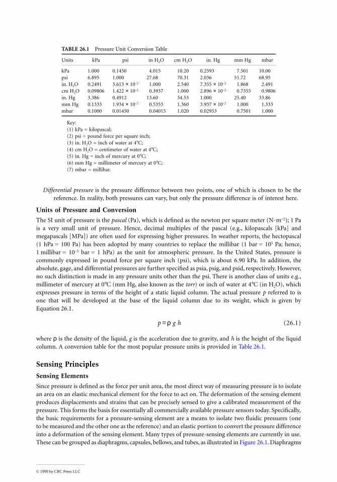
The SI unit of pressure is the pascal (Pa), which is defined as the newton per square meter (N·m–2); 1 Pais a very small unit of pressure. Hence, decimal multiples of the pascal (e.g., kilopascals [kPa] andmegapascals [MPa]) are often used for expressing higher pressures. In weather reports, the hectopascal(1 hPa = 100 Pa) has been adopted by many countries to replace the millibar (1 bar = 105 Pa; hence,1 millibar = 10–3 bar = 1 hPa) as the unit for atmospheric pressure. In the United States, pressure iscommonly expressed in pound force per square inch (psi), which is about 6.90 kPa. In addition, theabsolute, gage, and differential pressures are further specified as psia, psig, and psid, respectively. However,no such distinction is made in any pressure units other than the psi. There is another class of units e.g.,millimeter of mercury at 0°C (mm Hg, also known as the torr) or inch of water at 4°C (in H2O), whichexpresses pressure in terms of the height of a static liquid column. The actual pressure p referred to isone that will be developed at the base of the liquid column due to its weight, which is given byEquation 26.1.

(26.1)

where ρ is the density of the liquid, g is the acceleration due to gravity, and h is the height of the liquidcolumn. A conversion table for the most popular pressure units is provided in Table 26.1.

Sensing Principles

Sensing Elements

Since pressure is defined as the force per unit area, the most direct way of measuring pressure is to isolatean area on an elastic mechanical element for the force to act on. The deformation of the sensing elementproduces displacements and strains that can be precisely sensed to give a calibrated measurement of thepressure. This forms the basis for essentially all commercially available pressure sensors today. Specifically,the basic requirements for a pressure-sensing element are a means to isolate two fluidic pressures (oneto be measured and the other one as the reference) and an elastic portion to convert the pressure differenceinto a deformation of the sensing element. Many types of pressure-sensing elements are currently in use.These can be grouped as diaphragms, capsules, bellows, and tubes, as illustrated in Figure 26.1. Diaphragms

TABLE 26.1 Pressure Unit Conversion Table

Units kPa psi in H2O cm H2O in. Hg mm Hg mbar

kPa 1.000 0.1450 4.015 10.20 0.2593 7.501 10.00psi 6.895 1.000 27.68 70.31 2.036 51.72 68.95in. H2O 0.2491 3.613 × 10–2 1.000 2.540 7.355 × 10–2 1.868 2.491cm H2O 0.09806 1.422 × 10–2 0.3937 1.000 2.896 × 10–2 0.7355 0.9806in. Hg 3.386 0.4912 13.60 34.53 1.000 25.40 33.86mm Hg 0.1333 1.934 × 10–2 0.5353 1.360 3.937 × 10–2 1.000 1.333mbar 0.1000 0.01450 0.04015 1.020 0.02953 0.7501 1.000

Key:(1) kPa = kilopascal;(2) psi = pound force per square inch;(3) in. H2O = inch of water at 4°C;(4) cm H2O = centimeter of water at 4°C;(5) in. Hg = inch of mercury at 0°C;(6) mm Hg = millimeter of mercury at 0°C;(7) mbar = millibar.

p g h= ρ


are by far the most widely used of all sensing elements. A special form of tube, known as the Bourdontube, is curved or twisted along its length and has an oval cross-section. The tube is sealed at one endand tends to unwind or straighten when it is subjected to a pressure applied to the inside. In general,Bourdon tubes are designed for measuring high pressures, while capsules and bellows are usually formeasuring low pressures. A detailed description of these sensing elements can be found in [1].

FIGURE 26.1 Pressure-sensing elements: (a) flat diaphragm; (b) corrugated diaphragm; (c) capsule; (d) bellows;(e) straight tube; (f) C-shaped Bourdon tube; (g) twisted Bourdon tube; (h) helical Bourdon tube; (1) spiral Bourdontube.

Motion

Pressure

Motion

Pressure

Motion

Pressure

Motion

Pressure

Motion

PressurePressure

Motion

Motion

Pressure

(a) (b) (c)

(d) (e) (f)

(g) (h) (i)

Motion

Pressure

PressureMotion


Detection Methods

A detection means is required to convert the deformation of the sensing element into a pressure readout.In the simplest approach, the displacements of a sensing element can be amplified mechanically by leverand flexure linkages to drive a pointer over a graduated scale, for example, in the moving pointerbarometers. Some of the earliest pressure sensors employed a Bourdon tube to drive the wiper arm overa potentiometric resistance element. In linear-variable differential-transformer (LVDT) pressure sensors,the displacement of a Bourdon tube or capsule is used to move a magnetic core inside a coil assemblyto vary its inductance. In piezoelectric pressure sensors, the strains associated with the deformation of asensing element are converted into an electrical charge output by a piezoelectric crystal. Piezoelectricpressure sensors are useful for measuring high-pressure transient events, for example, explosive pressures.In vibrating-wire pressure sensors, a metal wire (typically tungsten) is stretched between a fixed anchorand the center of a diaphragm. The wire is located near a permanent magnet and is set into vibrationat its resonant frequency by an ac current excitation. A pressure-induced displacement of the diaphragmchanges the tension and therefore the resonant frequency of the wire, which is measured by the readoutelectronics. A detailed description of these and other types of detection methods can be found in [1].

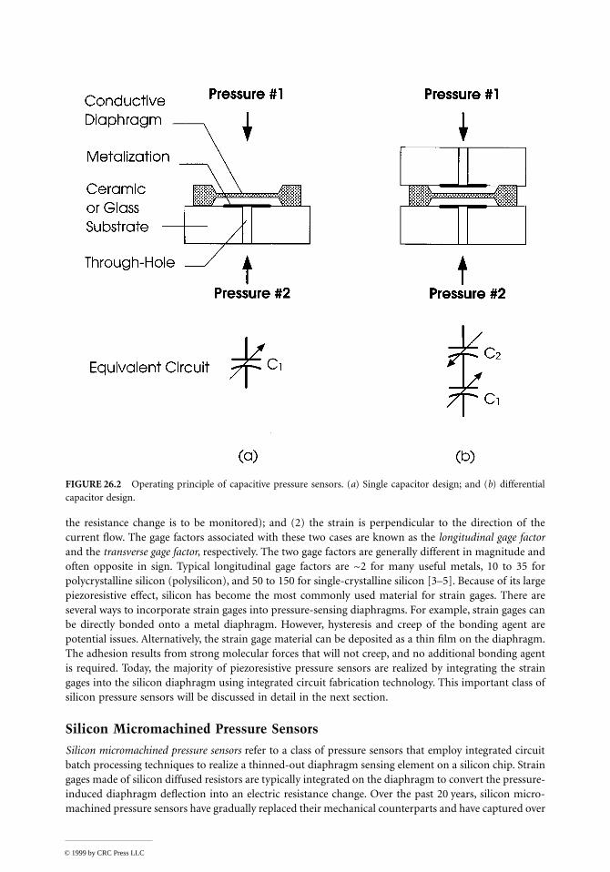
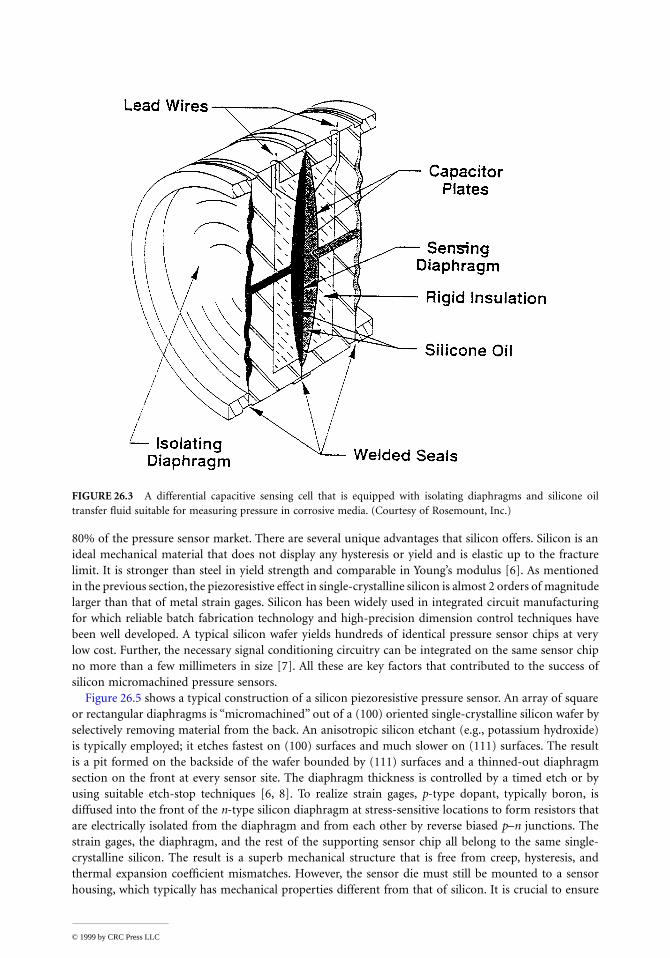
Capacitive Pressure Sensors.Many highly accurate (better than 0.1%) pressure sensors in use today have been developed using thecapacitive detection approach. Capacitive pressure sensors can be designed to cover an extremely widepressure range. Both high-pressure sensors with full-scale pressures above 107 Pa (a few thousand psi)and vacuum sensors (commonly referred to as capacitive manometers) usable for pressure measurementsbelow 10–3 Pa (10–5 torr) are commercially available. The principle of capacitive pressure sensors isillustrated in Figure 26.2. A metal or silicon diaphragm serves as the pressure-sensing element andconstitutes one electrode of a capacitor. The other electrode, which is stationary, is typically formed bya deposited metal layer on a ceramic or glass substrate. An applied pressure deflects the diaphragm, whichin turn changes the gap spacing and the capacitance [2]. In the differential capacitor design, the sensingdiaphragm is located in between two stationary electrodes. An applied pressure will cause one capacitanceto increase and the other one to decrease, thus resulting in twice the signal while canceling manyundesirable common mode effects. Figure 26.3 shows a practical design of a differential capacitive sensingcell that uses two isolating diaphragms and an oil fill to transmit the differential pressure to the sensingdiaphragm. The isolating diaphragms are made of special metal alloys that enable them to handlecorrosive fluids. The oil is chosen to set a predictable dielectric constant for the capacitor gaps whileproviding adequate damping to reduce shock and vibration effects. Figure 26.4 shows a rugged capacitivepressure sensor for industrial applications based on the capacitive sensing cell shown in Figure 26.3. Thecapacitor electrodes are connected to the readout electronics housing at the top. In general, with today’ssophisticated electronics and special considerations to minimize stray capacitances (that can degrade theaccuracy of measurements), a capacitance change of 10 aF (10–18 F) provided by a diaphragm deflectionof only a fraction of a nanometer is resolvable.

Piezoresistive Pressure Sensors.Piezoresistive sensors (also known as strain-gage sensors) are the most common type of pressure sensorin use today. Piezoresistive effect refers to a change in the electric resistance of a material when stressesor strains are applied. Piezoresistive materials can be used to realize strain gages that, when incorporatedinto diaphragms, are well suited for sensing the induced strains as the diaphragm is deflected by anapplied pressure. The sensitivity of a strain gage is expressed by its gage factor, which is defined as thefractional change in resistance, ∆R/R, per unit strain:

(26.2)

where strain ε is defined as ∆L/L, or the extension per unit length. It is essential to distinguish betweentwo different cases in which: (1) the strain is parallel to the direction of the current flow (along which

Gage factor = ( )∆R R ε


the resistance change is to be monitored); and (2) the strain is perpendicular to the direction of thecurrent flow. The gage factors associated with these two cases are known as the longitudinal gage factorand the transverse gage factor, respectively. The two gage factors are generally different in magnitude andoften opposite in sign. Typical longitudinal gage factors are ~2 for many useful metals, 10 to 35 forpolycrystalline silicon (polysilicon), and 50 to 150 for single-crystalline silicon [3–5]. Because of its largepiezoresistive effect, silicon has become the most commonly used material for strain gages. There areseveral ways to incorporate strain gages into pressure-sensing diaphragms. For example, strain gages canbe directly bonded onto a metal diaphragm. However, hysteresis and creep of the bonding agent arepotential issues. Alternatively, the strain gage material can be deposited as a thin film on the diaphragm.The adhesion results from strong molecular forces that will not creep, and no additional bonding agentis required. Today, the majority of piezoresistive pressure sensors are realized by integrating the straingages into the silicon diaphragm using integrated circuit fabrication technology. This important class ofsilicon pressure sensors will be discussed in detail in the next section.

Silicon Micromachined Pressure Sensors

Silicon micromachined pressure sensors refer to a class of pressure sensors that employ integrated circuitbatch processing techniques to realize a thinned-out diaphragm sensing element on a silicon chip. Straingages made of silicon diffused resistors are typically integrated on the diaphragm to convert the pressure-induced diaphragm deflection into an electric resistance change. Over the past 20 years, silicon micro-machined pressure sensors have gradually replaced their mechanical counterparts and have captured over

FIGURE 26.2 Operating principle of capacitive pressure sensors. (a) Single capacitor design; and (b) differentialcapacitor design.


80% of the pressure sensor market. There are several unique advantages that silicon offers. Silicon is anideal mechanical material that does not display any hysteresis or yield and is elastic up to the fracturelimit. It is stronger than steel in yield strength and comparable in Young’s modulus [6]. As mentionedin the previous section, the piezoresistive effect in single-crystalline silicon is almost 2 orders of magnitudelarger than that of metal strain gages. Silicon has been widely used in integrated circuit manufacturingfor which reliable batch fabrication technology and high-precision dimension control techniques havebeen well developed. A typical silicon wafer yields hundreds of identical pressure sensor chips at verylow cost. Further, the necessary signal conditioning circuitry can be integrated on the same sensor chipno more than a few millimeters in size [7]. All these are key factors that contributed to the success ofsilicon micromachined pressure sensors.

Figure 26.5 shows a typical construction of a silicon piezoresistive pressure sensor. An array of squareor rectangular diaphragms is “micromachined” out of a (100) oriented single-crystalline silicon wafer byselectively removing material from the back. An anisotropic silicon etchant (e.g., potassium hydroxide)is typically employed; it etches fastest on (100) surfaces and much slower on (111) surfaces. The resultis a pit formed on the backside of the wafer bounded by (111) surfaces and a thinned-out diaphragmsection on the front at every sensor site. The diaphragm thickness is controlled by a timed etch or byusing suitable etch-stop techniques [6, 8]. To realize strain gages, p-type dopant, typically boron, isdiffused into the front of the n-type silicon diaphragm at stress-sensitive locations to form resistors thatare electrically isolated from the diaphragm and from each other by reverse biased p–n junctions. Thestrain gages, the diaphragm, and the rest of the supporting sensor chip all belong to the same single-crystalline silicon. The result is a superb mechanical structure that is free from creep, hysteresis, andthermal expansion coefficient mismatches. However, the sensor die must still be mounted to a sensorhousing, which typically has mechanical properties different from that of silicon. It is crucial to ensure

FIGURE 26.3 A differential capacitive sensing cell that is equipped with isolating diaphragms and silicone oiltransfer fluid suitable for measuring pressure in corrosive media. (Courtesy of Rosemount, Inc.)


a high degree of stress isolation between the sensor housing and the sensing diaphragm that may otherwiselead to long-term mechanical drifts and undesirable temperature behavior. A common practice is tobond a glass wafer or a second silicon wafer to the back of the sensor wafer to reinforce the overallcomposite sensor die. This way, the interface stresses generated by the die mount will also be sufficientlyremote from the sensing diaphragm and will not seriously affect its stress characteristics. For gage ordifferential pressure sensing, holes must be provided through the carrier wafer prior to bonding that arealigned to the etch pits of the sensor wafer leading to the back of the sensing diaphragms. No throughholes are necessary for absolute pressure sensing. The wafer-to-wafer bonding is performed in a vacuumto achieve a sealed reference vacuum inside the etch pit [6, 9]. Today’s silicon pressure sensors are availablein a large variety of plastic, ceramic, metal can, and stainless steel packages (some examples are shownin Figure 26.6). Many are suited for printed circuit board mounting. Others have isolating diaphragmsand transfer fluids for handling corrosive media. They can be readily designed for a wide range ofindustrial, medical, automotive, aerospace, and military applications.

Silicon Piezoresistive Pressure Sensor Limitations

Despite the relatively large piezoresistive effects in silicon strain gages, the full-scale resistance change istypically only 1% to 2% of the resistance of the strain gage (which yields an unamplified voltage outputof 10 mV/V to 20 mV/V). To achieve an overall accuracy of 0.1% of full scale, for example, the combinedeffects of mechanical and electrical repeatability, hysteresis, linearity, and stability must be controlled orcompensated to within a few parts per million (ppm) of the gage resistance. Furthermore, silicon straingages are also very temperature sensitive and require careful compensations. There are two primarysources of temperature drifts: (1) the temperature coefficient of resistance of the strain gages (from0.06%/oC to 0.24%/oC); and (2) the temperature coefficient of the gage factors (from –0.06%/oC to

FIGURE 26.4 A rugged capacitive pressure sensor product for industrial applications. It incorporates the sensingcell shown in Figure 26.3. Readout electronics are contained in the housing at the top. (Courtesy of Rosemount, Inc.)


FIGURE 26.5 A cut-away view showing the typical construction of a silicon piezoresistive pressure sensor.

FIGURE 26.6 Examples of commercially available packages for silicon pressure sensors. Shown in the photo aresurface-mount units, dual-in-line (DIP) units, TO-8 metal cans, and stainless steel units with isolating diaphragms.(Courtesy of EG&G IC Sensors.)


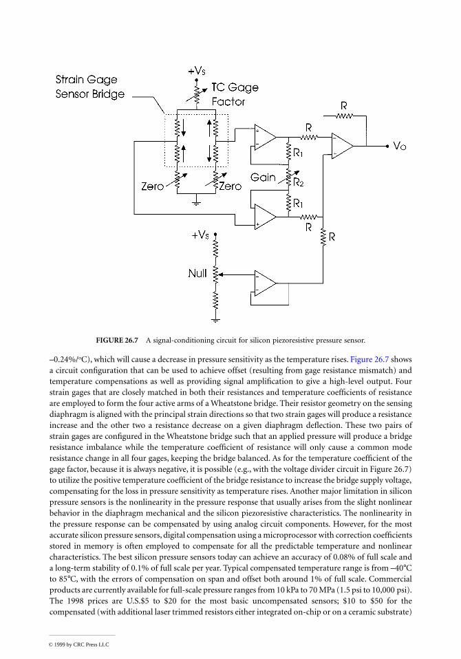
–0.24%/oC), which will cause a decrease in pressure sensitivity as the temperature rises. Figure 26.7 showsa circuit configuration that can be used to achieve offset (resulting from gage resistance mismatch) andtemperature compensations as well as providing signal amplification to give a high-level output. Fourstrain gages that are closely matched in both their resistances and temperature coefficients of resistanceare employed to form the four active arms of a Wheatstone bridge. Their resistor geometry on the sensingdiaphragm is aligned with the principal strain directions so that two strain gages will produce a resistanceincrease and the other two a resistance decrease on a given diaphragm deflection. These two pairs ofstrain gages are configured in the Wheatstone bridge such that an applied pressure will produce a bridgeresistance imbalance while the temperature coefficient of resistance will only cause a common moderesistance change in all four gages, keeping the bridge balanced. As for the temperature coefficient of thegage factor, because it is always negative, it is possible (e.g., with the voltage divider circuit in Figure 26.7)to utilize the positive temperature coefficient of the bridge resistance to increase the bridge supply voltage,compensating for the loss in pressure sensitivity as temperature rises. Another major limitation in siliconpressure sensors is the nonlinearity in the pressure response that usually arises from the slight nonlinearbehavior in the diaphragm mechanical and the silicon piezoresistive characteristics. The nonlinearity inthe pressure response can be compensated by using analog circuit components. However, for the mostaccurate silicon pressure sensors, digital compensation using a microprocessor with correction coefficientsstored in memory is often employed to compensate for all the predictable temperature and nonlinearcharacteristics. The best silicon pressure sensors today can achieve an accuracy of 0.08% of full scale anda long-term stability of 0.1% of full scale per year. Typical compensated temperature range is from –40°Cto 85°C, with the errors of compensation on span and offset both around 1% of full scale. Commercialproducts are currently available for full-scale pressure ranges from 10 kPa to 70 MPa (1.5 psi to 10,000 psi).The 1998 prices are U.S.$5 to $20 for the most basic uncompensated sensors; $10 to $50 for thecompensated (with additional laser trimmed resistors either integrated on-chip or on a ceramic substrate)

FIGURE 26.7 A signal-conditioning circuit for silicon piezoresistive pressure sensor.


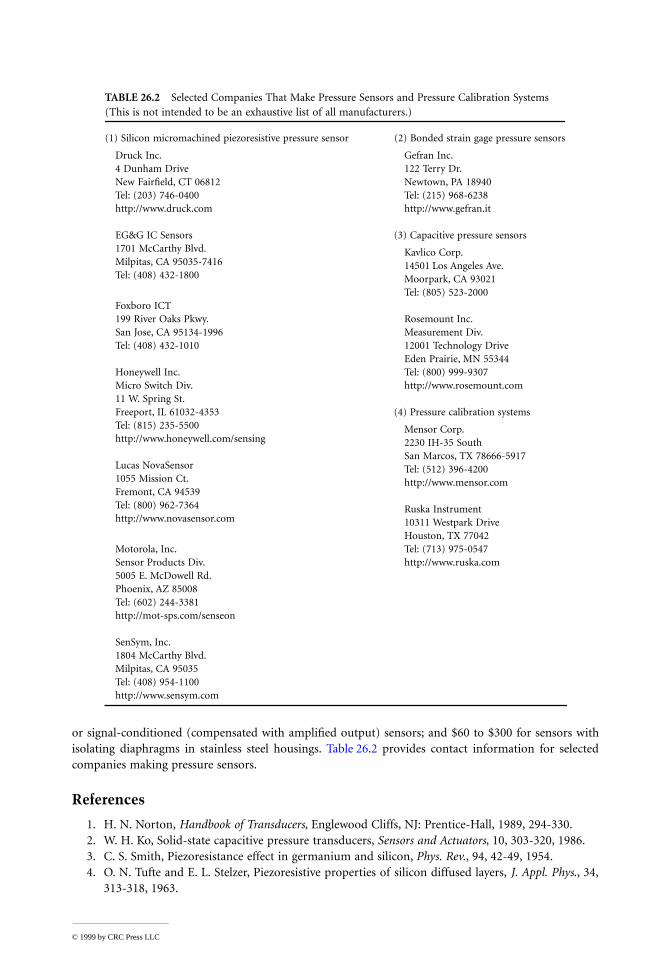
or signal-conditioned (compensated with amplified output) sensors; and $60 to $300 for sensors withisolating diaphragms in stainless steel housings. Table 26.2 provides contact information for selectedcompanies making pressure sensors.

References

1. H. N. Norton, Handbook of Transducers, Englewood Cliffs, NJ: Prentice-Hall, 1989, 294-330.2. W. H. Ko, Solid-state capacitive pressure transducers, Sensors and Actuators, 10, 303-320, 1986.3. C. S. Smith, Piezoresistance effect in germanium and silicon, Phys. Rev., 94, 42-49, 1954.4. O. N. Tufte and E. L. Stelzer, Piezoresistive properties of silicon diffused layers, J. Appl. Phys., 34,

313-318, 1963.

TABLE 26.2 Selected Companies That Make Pressure Sensors and Pressure Calibration Systems (This is not intended to be an exhaustive list of all manufacturers.)

(1) Silicon micromachined piezoresistive pressure sensor (2) Bonded strain gage pressure sensors

Druck Inc.4 Dunham DriveNew Fairfield, CT 06812Tel: (203) 746-0400http://www.druck.com

Gefran Inc.122 Terry Dr.Newtown, PA 18940Tel: (215) 968-6238http://www.gefran.it

EG&G IC Sensors1701 McCarthy Blvd.Milpitas, CA 95035-7416Tel: (408) 432-1800

(3) Capacitive pressure sensors

Kavlico Corp.14501 Los Angeles Ave.Moorpark, CA 93021Tel: (805) 523-2000

Foxboro ICT199 River Oaks Pkwy.San Jose, CA 95134-1996Tel: (408) 432-1010

Rosemount Inc.Measurement Div.12001 Technology DriveEden Prairie, MN 55344Tel: (800) 999-9307http://www.rosemount.com

Honeywell Inc.Micro Switch Div.11 W. Spring St.Freeport, IL 61032-4353Tel: (815) 235-5500http://www.honeywell.com/sensing

(4) Pressure calibration systems

Mensor Corp.2230 IH-35 SouthSan Marcos, TX 78666-5917Tel: (512) 396-4200http://www.mensor.com

Lucas NovaSensor1055 Mission Ct.Fremont, CA 94539Tel: (800) 962-7364http://www.novasensor.com

Ruska Instrument10311 Westpark DriveHouston, TX 77042Tel: (713) 975-0547http://www.ruska.com

Motorola, Inc.Sensor Products Div.5005 E. McDowell Rd.Phoenix, AZ 85008Tel: (602) 244-3381http://mot-sps.com/senseon

SenSym, Inc.1804 McCarthy Blvd.Milpitas, CA 95035Tel: (408) 954-1100http://www.sensym.com


5. D. Schubert, W. Jenschke, T. Uhlig, and F. M. Schmidt, Piezoresistive properties of polycrystallineand crystalline silicon films, Sensors and Actuators, 11, 145-155, 1987.

6. K. E. Petersen, Silicon as a mechanical material, IEEE Proc., 70, 420-457, 1982.7. R. F. Wolffenbuttel (ed.), Silicon Sensors and Circuits: On-Chip Compatibility, London: Chapman

& Hall, 1996, 171-210.8. H. Seidel, The mechanism of anisotropic silicon etching and its relevance for micromachining,

Tech. Dig., Transducers ’87, Tokyo, Japan, June 1987, 120-125.9. E. P. Shankland, Piezoresistive silicon pressure sensors, Sensors, 22-26, Aug. 1991.

Further Information

R. S. Muller, R. T. Howe, S. D. Senturia, R. L. Smith, and R. M. White (eds.), Microsensors, New York:IEEE Press, 1991, provides an excellent collection of papers on silicon microsensors and siliconmicromachining technologies.

R. F. Wolffenbuttel (ed.), Silicon Sensors and Circuits: On-Chip Compatibility, London: Chapman & Hall,1996, provides a thorough discussion on sensor and circuit integration.

ISA Directory of Instrumentation On-Line (http://www.isa.org) from the Instrument Society of Americamaintains a list of product categories and active links to many sensor manufacturers.

26.2 Vacuum Measurement

Ron Goehner, Emil Drubetsky, Howard M. Brady, and William H. Bayles, Jr.

Background and History of Vacuum Gages

To make measurements in the vacuum region, one must possess a knowledge of the expected pressurerange required by the processes taking place in the vacuum chamber as well as the accuracy and/orrepeatability of the measurement required for the process. Typical vacuum systems require that manyorders of magnitude of pressures must be measured. In many applications, the pressure range may be 8orders of magnitude, or from atmospheric (1.01 × 105 Pa, 760 torr) to 1 × 10–3 Pa (7.5 × 10–6 torr).

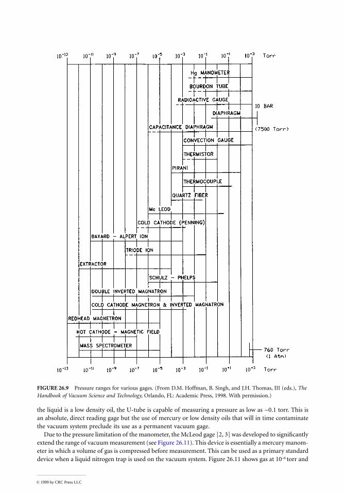
For semiconductor lithography, high-energy physics experiments and surface chemistry, ultimatevacuum of 7.5 × 10–9 torr and much lower are required (a range of 11 orders of magnitude belowatmospheric pressure). One gage will not give reasonable measurements over such large pressure ranges.Over the past 50 years, vacuum measuring instruments (commonly called gages) have been developedthat used transducers (or sensors) which can be classified as either direct reading (usually mechanical)or indirect reading [1] (usually electronic). Figure 26.8 shows vacuum gages typically in current use.When a force on a surface is used to measure pressure, the gages are mechanical and are called directreading gages, whereas when any property of the gas that changes with density is measured by electronicmeans, they are called indirect reading gages. Figure 26.9 shows the range of operating pressure for varioustypes of vacuum gages.

Direct Reading Gages

A subdivision of direct reading gages can be made by dividing them into those that utilize a liquid walland those that utilize a solid wall. The force exerted on a surface from the pressure of thermally agitatedmolecules and atoms is used to measure the pressure.

Liquid Wall Gages

The two common gages that use a liquid wall are the manometer and the McLeod gage. The liquidcolumn manometer is the simplest type of vacuum gage. It consists of a straight or U-shaped glass tube


evacuated and sealed at one end and filled partly with mercury or a low vapor pressure liquid such asdiffusion pump oil (See Figure 26.10). In the straight tube manometer, as the space above the mercuryis evacuated, the length of the mercury column decreases. In the case of the U-tube, as the free end isevacuated, the two columns approach equal height. The pressure at the open end is measured by thedifference in height of the liquid columns. If the liquid is mercury, the pressure is directly measured inmm of Hg (torr). The manometer is limited to pressures equal to or greater than ~1 torr (133 Pa). If

FIGURE 26.8 Classification of pressure gages. (From D.M. Hoffman, B. Singh, and J.H. Thomas, III (eds.), The Handbook of Vacuum Science and Technology, Orlando, FL: Academic Press, 1998. With permission.)


the liquid is a low density oil, the U-tube is capable of measuring a pressure as low as ~0.1 torr. This isan absolute, direct reading gage but the use of mercury or low density oils that will in time contaminatethe vacuum system preclude its use as a permanent vacuum gage.

Due to the pressure limitation of the manometer, the McLeod gage [2, 3] was developed to significantlyextend the range of vacuum measurement (see Figure 26.11). This device is essentially a mercury manom-eter in which a volume of gas is compressed before measurement. This can be used as a primary standarddevice when a liquid nitrogen trap is used on the vacuum system. Figure 26.11 shows gas at 10–6 torr and

FIGURE 26.9 Pressure ranges for various gages. (From D.M. Hoffman, B. Singh, and J.H. Thomas, III (eds.), The Handbook of Vacuum Science and Technology, Orlando, FL: Academic Press, 1998. With permission.)


a compression ratio of 10+7. In this example, the difference of the columns will be 10 mm. Extreme caremust be taken not to break the glass and expose the surroundings to the mercury. The McLeod Gage isan inexpensive standard but should only be used by skilled and careful technicians. The gage will give afalse low reading unless precautions are taken to ensure that any condensible vapors present are removedby liquid nitrogen trapping.

FIGURE 26.10 Mercury manometers. (From W.H. Bayles, Jr., Fundamentals of Vacuum Measurement, Calibration and Certification, Industrial Heating, October 1992. With permission.)


Solid Wall Gages

There are two major mechanical solid wall gage types: capsule and diaphragm.

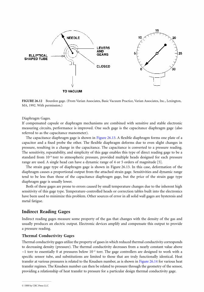
Bourdon Gages.The capsule-type gages depend on the deformation of the capsule with changing pressure and theresultant deflection of an indicator. Pressure gages using this principle measure pressures above atmo-spheric to several thousand psi and are commonly used on compressed gas systems. This type of gage isalso used at pressures below atmospheric, but the sensitivity is low. The Bourdon gage (Figure 26.12), isused as a moderate vacuum gage. In this case, the capsule is in the form of a thin-walled tube bent in acircle, with the open end attached to the vacuum system with a mechanism and a pointer attached tothe other end. The atmospheric pressure deforms the tube; a linear indication of the pressure is giventhat is independent of the nature of the gas. Certain manufacturers supply capsule gages capable ofmeasuring pressures as low as 1 torr. These gages are rugged, inexpensive, and simple to use and can bemade of materials inert to corrosive vapors. Since changing atmospheric pressure causes inaccuracies inthe readings, compensated versions of the capsule and Bourdon gage have been developed that improvethe accuracy [4].

FIGURE 26.11 McLeod gage. (From D.M. Hoffman, B. Singh, and J.H. Thomas, III (eds.), The Handbook of Vacuum Science and Technology, Orlando, FL: Academic Press, 1998. With permission.)


Diaphragm Gages.If compensated capsule or diaphragm mechanisms are combined with sensitive and stable electronicmeasuring circuits, performance is improved. One such gage is the capacitance diaphragm gage (alsoreferred to as the capacitance manometer).

The capacitance diaphragm gage is shown in Figure 26.13. A flexible diaphragm forms one plate of acapacitor and a fixed probe the other. The flexible diaphragm deforms due to even slight changes inpressure, resulting in a change in the capacitance. The capacitance is converted to a pressure reading.The sensitivity, repeatability, and simplicity of this gage enables this type of direct reading gage to be astandard from 10–6 torr to atmospheric pressure, provided multiple heads designed for each pressurerange are used. A single head can have a dynamic range of 4 or 5 orders of magnitude [5].

The strain gage type of diaphragm gage is shown in Figure 26.13. In this case, deformation of thediaphragm causes a proportional output from the attached strain gage. Sensitivities and dynamic rangetend to be less than those of the capacitance diaphragm gage, but the price of the strain gage typediaphragm gage is usually lower.

Both of these gages are prone to errors caused by small temperature changes due to the inherent highsensitivity of this gage type. Temperature-controlled heads or correction tables built into the electronicshave been used to minimize this problem. Other sources of error in all solid wall gages are hysteresis andmetal fatigue.

Indirect Reading Gages

Indirect reading gages measure some property of the gas that changes with the density of the gas andusually produces an electric output. Electronic devices amplify and compensate this output to providea pressure reading.

Thermal Conductivity Gages

Thermal conductivity gages utilize the property of gases in which reduced thermal conductivity correspondsto decreasing density (pressure). The thermal conductivity decreases from a nearly constant value above~1 torr to essentially 0 at pressures below 10–2 torr. The gage controllers are designed to work with aspecific sensor tube, and substitutions are limited to those that are truly functionally identical. Heattransfer at various pressures is related to the Knudsen number, as is shown in Figure 26.14 for various heattransfer regimes. The Knudsen number can then be related to pressure through the geometry of the sensor,providing a relationship of heat transfer to pressure for a particular design thermal conductivity gage.

FIGURE 26.12 Bourdon gage. (From Varian Associates, Basic Vacuum Practice, Varian Associates, Inc., Lexington, MA, 1992. With permission.)


Pirani Gages.The Pirani gage is perhaps the oldest indirect gage that is still used today. In operation, a sensing filamentcarrying current and producing heat is surrounded by the gas to be measured. As the pressure changes,the thermal conductivity changes, thus varying the temperature of the sensing filament. The temperaturechange causes a change in the resistance of the sensing filament. The sensing filament is usually one legof a Wheatstone bridge. The bridge can be operated so that the voltage is varied to keep the bridgebalanced; that is, the resistance of the sensing filament is kept constant.

This method is called the constant temperature method and is deemed the fastest, most sensitive, andmost accurate. To reduce the effect of changing ambient temperature, an identical filament sealed off atvery low pressure is placed in the leg adjacent to the sensing filament as a balancing resistor. Because ofits high thermal resistance coefficient, the filament material is usually a thin tungsten wire. It has beendemonstrated that a 10 W light bulb works quite well [6]. (see Figure 26.15.)

A properly designed, compensated Pirani gage with sensitive circuitry is capable of measuring to10–4 torr. However, the thermal conductivity of gases varies with the gas being measured, causing avariation in gage response. These variations can be as large as a factor of 5 at low pressures and as highas 10 at high pressures (see Figure 26.16). Correction for these variations can be made on the calibrationcurves supplied by the manufacturer if the composition of the gas is known. Operation in the presenceof high partial pressures of organic molecules such as oils is not recommended.

FIGURE 26.13 Diaphragm gage. (From W.H. Bayles, Jr., Fundamentals of Vacuum Measurement, Calibration and Certification, Industrial Heating, October 1992. With permission.)


Thermistor Gages.In the thermistor gage, a thermistor is used as one leg of a bridge circuit. The inverse resistive charac-teristics of the thermistor element unbalances the bridge as the pressure changes, causing a correspondingchange in current. Sensitive electronics measure the current and are calibrated in pressure units. The

FIGURE 26.14 Heat transfer regimes in a thermal conductivity gage.

FIGURE 26.15 Pirani gage.

103 101 10-1 10-3

Conduction

Hea

t Tra

nsfe

r

Radiation

Convection

Kn = l/d

M

RMR1

R3

R2

R4

CompensationTube

GaugeTube

Vdc


thermistor gage measures approximately the same pressure range as the thermocouple.The exact calibrationdepends on the the gas measured. In a well-designed bridge circuit, the plot of current vs. pressure is practicallylinear in the range 10–3 to 1 torr [7]. Modern thermistor gages use constant-temperature techniques.

Thermocouple Gages.Another example of an indirect reading thermal conductivity gage is the thermocouple gage. This is arelatively inexpensive device with proven reliability and a wide range of applications. In the thermocouplegage, a filament of resistance alloy is heated by the passage of a constant current (see Figure 26.17). Athermocouple is welded to the midpoint of the filament or preferably to a conduction bridge at the centerof the heated filament. This provides a means of directly measuring the temperature. With a constantcurrent through the filament, the temperature increases as the pressure decreases as there are fewermolecules surrounding the filament to carry the heat away. The thermocouple output voltage increasesas a result of the increased temperature and varies inversely with the pressure. The thermocouple gagecan also be operated in the constant-temperature mode.

Gas composition effects apply to all thermal conductivity gages. The calibration curves for a typicalthermocouple gage are shown in Figure 26.18. The thermocouple gage can be optimized for operationin various pressure ranges. Operation of the thermocouple gage in high partial pressures of organicmolecules such as oils should be avoided. One manufacturer pre-oxidizes the thermocouple sensor forstability in “dirty” environments and for greater interchangeability in clean environments.

Convection Gages.Below 1 torr a significant change in thermal conductivity occurs as the pressure changes. Thus, thethermal conductivity gage is normally limited to 1 torr.

At pressures above 1 torr, there is, in most gages, a small contribution to heat transfer caused byconvection. Manufacturers have developed gages that utilize this convection effect to extend the usable

FIGURE 26.16 Calibration curves for the Pirani gage. (Reprinted with permission from Leybold-Herqeus GMblt, Köhn, Germany.)


range to atmospheric pressure and slightly above [8–12]. Orientation of a convection gage is critical becausethis convection heat transfer is highly dependent on the orientation of the elements within the gage.

The Convectron™ uses the basic structure of the Pirani with special features to enhance convectioncooling in the high-pressure region [13]. To utilize the gage above 1 torr (133 Pa), the sensor tube mustbe mounted with its major axis in a horizontal position. If the only area of interest is below 1 torr, thetube can be mounted in any position. As mentioned above, the gage controller is designed to be usedwith a specific model sensor tube; because extensive use is made of calibration curves and look-up tablesstored in the controller, no substitution is recommended.

The Televac convection gage uses the basic structure of the thermocouple gage except that two ther-mocouples are used [14]. As in any thermocouple gage, the convection gage measures the pressure bydetermining the heat loss from a fine wire maintained at constant temperature. The response of thesensor depends on the gas type. A pair of thermocouples is mounted a fixed distance from each other(see Figure 26.19). The one mounted lower is heated to a constant temperature by a variable currentpower supply. Power is pulsed to this lower thermocouple and the temperature is measured betweenheating pulses. The second (upper) thermocouple measures convection effects and also compensates forambient temperature. At pressures below ~2 torr (270 Pa) the temperature in the upper thermocoupleis negligible. The gage tube operates as a typical thermocouple in the constant-temperature mode. Above2 torr, convective heat transfer causes heating of the upper thermocouple. The voltage output is subtractedfrom that of the lower thermocouple, thus requiring more current to maintain the wire temperature.Consequently, the range of pressure that can be measured (via current change) is extended to atmosphericpressure (see Figure 26.20). Orientation of the sensor is with the axis vertical.

The use of convection gages with process control electronics allows for automatic pump-down withthe assurance that the system will neither open under vacuum nor be subject to over-pressure duringbackfill to atmospheric pressure. These gages, with their controllers, are relatively inexpensive. In oil-freesystems, they afford long life and reproducible results.

FIGURE 26.17 Thermocouple gage. (Reprinted with permission of Televac Division, The Fredericks Co., Hunting-don Valley, PA.)


Hot Cathode Ionization Gages

Hot cathode ionization gage designs consist of triode gages, Bayard-Alpert gages, and others.

Triode Hot Cathode Ionization Gages.For over 80 years, the triode electron tube has been used as an indirect way to measure vacuum [15, 16].A typical triode connection is as an amplifier, as is shown in Figure 26.21. A brief description of itsoperation is given here, but more rigorous treatment of triode performance is given in [17–20]. However,if the triode is connected as in Figure 26.22 so that the grid is positive and the plate is negative withrespect to the filament, then the ion current collected by the plate for the same electron current to thegrid is greatly increased [21].

Today, the triode gage is used in this higher sensitivity mode. Many investigators have shown that alinear change in molecular density (pressure) results in a linear change in ion current [15, 21, 22]. Thislinearity allows a sensitivity factor S to be defined such that:

(26.3)

where Ii = Ion current (A)Ie = Electron current (A)P = PressureS = Sensitivity (in units of reciprocal pressure)

FIGURE 26.18 Calibration curves for the thermocouple gage. (Reprinted with permission from Televac Division, The Fredericks Co., Huntingdon Valley, PA.)

I S I Pi e= × ×


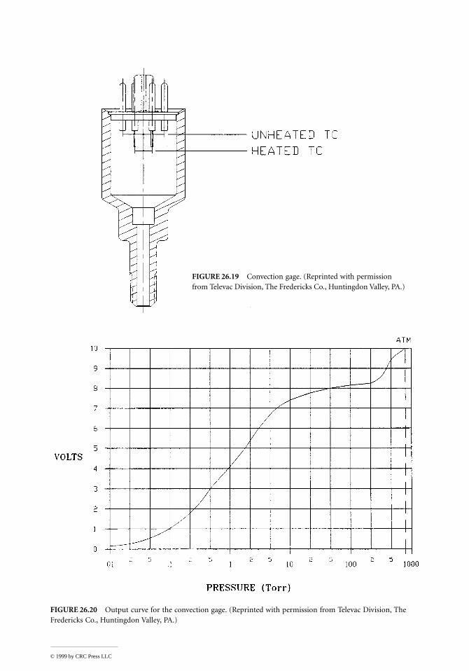
FIGURE 26.20 Output curve for the convection gage. (Reprinted with permission from Televac Division, The Fredericks Co., Huntingdon Valley, PA.)

FIGURE 26.19 Convection gage. (Reprinted with permission from Televac Division, The Fredericks Co., Huntingdon Valley, PA.)


FIGURE 26.21 Typical triode connection.

FIGURE 26.22 Alternative triode connection.


Additional details are found in [23–25]. In nearly all cases, except at relatively high pressures, the triodegage has been replaced by the Bayard–Alpert gage.

Bayard–Alpert Hot Cathode Ionization Gages.It became apparent that the pressure barrier observed at 10–8 torr was caused by a failure in measurementrather than pumping [26, 27]. A solution to this problem was proposed by Bayard and Alpert [28] thatis now the most widely used gage for general UHV measurement.

The Bayard–Alpert gage is similar to a triode gage but has been redesigned so that only a small quantityof the internally generated X-rays strike the collector. The primary features of the Bayard–Alpert gageand its associated circuit are shown in Figures 26.23 and 26.24. The cathode has been replaced by a thincollector located at the center of the grid, and the cathode filament is now outside and several millimetersaway from the grid. The Bayard–Alpert design utilizes the same controller as the triode gage, with

FIGURE 26.23 Bayard–Alpert hot cathode ionization gage.


corrections for sensitivity differences between the gage designs. When a hot filament gage is exposed tohigh pressures, burn-out of the tungsten filaments often occurs. To prevent this, platinum metals werecoated with refractory oxides to allow the gage to withstand sudden exposure to atmosphere with thefilament hot [29, 30]. Typical materials include either thoria or yttria coatings on iridium. Bayard–Alpertand triode gages of identical structure and dimensions but with different filaments (i.e., tungsten vs.thoria iridium)were observed to have different sensitivities, with the tungsten filament versions being20% to 40% more sensitive than the iridium of the same construction.

The lowest pressure that can be measured is limited by low energy X-rays striking the ion collectorand emitting electrons. Several methods to reduce this X-ray limit were developed. Gage designs withvery small diameter collectors have been made that extend the high vacuum range down to 10–12 torr,but accuracy was lost at the high pressures [31, 32].

The modulated gage was designed by Redhead [33] with an extra electrode near the ion collector. Inthis configuration, the X-ray current could be subtracted by measuring the ion current at two modulatorpotentials, thus increasing the range to 5 × 10–12. Other gages use suppressor electrodes in front of theion collector [34, 35].

The extractor gage (Figure 26.25) is the most widely used UHV hot cathode gage for those who needto measure 10–12 torr [36]. In this gage, the ions are extracted out of the ionizing volume and deflectedor focused onto a small collector. More recent designs have been developed [37, 38]. The use of a channelelectron multiplier [39] has reduced the low pressure limit to 10–15 torr.

The Bayard–Alpert gage suffers from some problems, however. The ion current is geometry dependent.Investigators have reported on the sensitivity variations, inaccuracy, and instability of Bayard-Alpert gageswith widely differing results [40–46, 49, 50, 56]. Investigators have developed ways to reduce or eliminatesome of these problems [47, 48].

FIGURE 26.24 Bayard–Alpert gage configuration.


Cold Cathode Ionization Gages

To measure pressures below 10–3 torr, Penning [51] developed the cold cathode discharge gage. Below10–3 torr, the mean free path is so high that little ionization takes place. The probability of ionizationwas increased by placing a magnetic field parallel to the paths of ions and electrons to force these particlesinto helical trajectory.

This gage consists of two parallel cathodes and an anode, which is placed midway between them (seeFigure 26.26). The anode is a circular or rectangular loop of metal wire whose plane is parallel to thatof the cathodes. A few kilovolts potential difference is maintained between the anode and the cathodes.

FIGURE 26.25 Extractor ionization gage. F, filament; G, grid; S, shield; IR, iron reflector; IC, ion collector.

FIGURE 26.26 Penning gages. ([Left] From J.F. O’Hanlon, A User’s Guide to Vacuum Technology, New York: John Wiley & Sons, 1980, 47. With permission. [Right] Reprinted with permission from Televac Division, The Fredericks Co., Huntingdon Valley, PA.)


Furthermore, a magnetic field is applied between the cathodes by a permanent magnet usually externalto the gage body. Electrons emitted from either of the two cathodes must travel in helical paths due tothe magnetic field eventually reaching the anode, which carries a high positive charge. During the travelalong this long path, many electrons collide with the molecules of the gas, thus creating positive ionsthat travel more directly to the cathodes. The ionization current thus produced is read out on a sensitivecurrent meter as pressure.

This is a rugged gage used for industrial applications such as in leak detectors, vacuum furnaces, electronbeam welders, and other industrial processes. The Penning gage is rugged, simple, and inexpensive. Its rangeis typically 10–3 torr to 10–6 torr, and some instability and lack of accuracy has been observed [52]. Themagnetron design [53] and the inverted magnetron design [54] extended the low pressure range to 10–12

Torr [55] or better. These improvements produced a better gage but instability, hysterisis, and startingproblems remain [57, 58]. Magnetrons currently in use are simpler and do not use an auxiliary cathode.

More recently, a double inverted magnetron was introduced [59]. This gage has greater sensitivity(amp/torr) than the other types (see Figure 26.27). It has been operated successfully at ~1 × 10–11 torr.The gage consists of two axially magnetized, annular-shaped magnets (1) placed around a cylinder (2)so that the north pole of one magnet faces the north pole of the other one. A nonmagnetic spacer (3) isplaced between the two magnets and thin shims (4) are used to focus the magnetic fields. This gage hasbeen operated to date at 10–11 torr, and stays ignited and reignites quickly when power is restored at thispressure. Essentially instantaneous reignition has been demonstrated by use of radioactive triggering [60].

Resonance Gages

One example of a resonance-type vacuum gage is the quartz friction vacuum gage [61]. A quartz oscillatorcan be built to measure pressure by a shift in resonance frequency caused by static pressure of thesurrounding gas or by the increased power required to maintain a constant amplitude. Its range is fromnear atmospheric pressure to about 0.1 torr. A second method is to measure the resonant electricalimpedance of a tuning fork oscillator. Test results for this device show an accuracy within ±10% forpressure from 10–3 torr to 103 torr. There is little commercial use to date for these devices.

FIGURE 26.27 Double inverted magnetron. (Reprinted with permission from Televac Division, The Fredericks Co., Huntingdon Valley, PA.)


Molecular Drag (Spinning Rotor) Gages

Meyer [62] and Maxwell [63] introduced the idea of measuring pressure by means of the molecular dragof rotating devices in 1875. The rotors of these devices were tethered to a wire or thin filament. The gagewas further enhanced by Holmes [64], who introduced the concept of the magnetic rotor suspension,leading to the spinning rotor gage. Nearly 10 years later, Beams et al. [65] disclosed the use of a magnet-ically levitated, rotating steel ball to measure pressure at high vacuum. Fremerey [66] reported on thehistorical development of this gage.

The molecular drag gage (MDG), often referred to as the spinning rotor gage, received wider acceptanceafter its commercial introduction in 1982 [67]. It is claimed to be more stable than other gages at lowerpressures [68].

The principle of operation of the modern MDG is based on the fact that the rate of change of theangular velocity of a freely spinning ball is proportional to the gas pressure and inversely proportionalto the mean molecular velocity. When the driving force is removed, the angular velocity is determinedby measuring the ac voltage induced in the pickup coils by the magnetic moment of the ball (seeFigure 26.28).

In current practice, a small rotor (steel ball bearing) about 4.5 mm in diameter is magnetically levitatedand spun up to about 400 Hz by induction. The ball, enclosed in a thimble connected to the vacuumsystem, is allowed to coast by turning off the inductive drive. Then, the time of a revolution of the ballis measured by timing the signal induced in a set of pickup coils by the rotational component of theball’s magnetic moment. Gas molecules will exert a drag on the ball, slowing it at a rate set by the pressureP, its molecular mass m, temperature T, and the coefficient of momentum transfer σ, between the gasand the ball. A perfectly smooth ball would have a value of unity. There is also a pressure-independentresidual drag (RD) caused by eddy current losses in the ball and surrounding structure. There will alsobe temperature effects that will cause the ball diameter and moment of inertia to change.

The pressure in the region of molecular flow is given by:

(26.4)

Note: Some sources include the term

where ρ = Density of the rotora = Radius of the rotorω′/ω = Fractional rate of slowing of the rotor–c = Mean gas molecular velocityα = Linear coefficient of expansion of the ballT′ = Rate of change of the ball’s temperature

All of the terms in the first part of the equation can be readily determined except for the accommodationcoefficient σ, which depends on the surface of the ball and the molecular adhesion between the gas andthe surface of the ball. The accommodation coefficient σ must be determined by calibration of the MDGagainst a known pressure standard or, if repeatability is more important than the highest accuracy, byassuming a value of 1 for σ. Measurements of σ on many balls over several years have been repeatedlyperformed by Dittman et al. [68]. The values obtained ranged from 0.97 to 1.06 for 68 visually smoothballs, so using a value of 1 for σ would not introduce a large error and would allow the MDG to beconsidered a primary standard (Fremerey [66]).

The controller [68] contains the electronics to power and regulate the suspension and drive, detectand amplify the signal from the pickup coils, and then time the rotation of the ball. It also contains adata processor that stores the calibration data and computes the pressure.

Pa c T= π − ′ − − ′

ρ

σω α

ω10

2

eff

RD

8kT ′( )πm( )

----------------


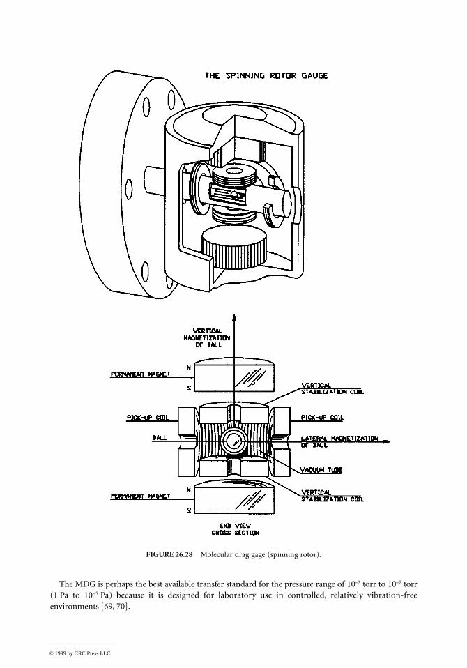
The MDG is perhaps the best available transfer standard for the pressure range of 10–2 torr to 10–7 torr(1 Pa to 10–5 Pa) because it is designed for laboratory use in controlled, relatively vibration-freeenvironments [69, 70].

FIGURE 26.28 Molecular drag gage (spinning rotor).


Partial Pressure Measurements and Mass Spectrometers

The theory and practical applications of partial pressure measurements and mass spectrometers arediscussed in detail in the literature [76]; however, an overview is presented herein [78].

A simple device for measuring the partial pressure of nitrogen as well as the total pressure in a vacuumsystem is the residual nitrogen analyzer (RNA). Operating in high vacuum, it is used to detect leaks ina vacuum system. It is effective because various gases are pumped at different rates and nitrogen is readilypumped, leaving a much lower percentage than is present at atmospheric pressure. Thus, the presenseof a significant percentage of nitrogen at high vacuum indicates an air leak. The RNA consists of a coldcathode gage with an optical filter and a photomultiplier tube. Since ionization in the cold cathode tubeproduces light and the color is determined by the gases present, the RNA filters out all except for thatcorresponding to nitrogen and is calibrated to give the partial pressure of nitrogen.

A more complex device to measure the partial pressure of many gases in a vacuum chamber is themass spectrometer-type residual gas analyzer (RGA). This device comes in many forms and several sizes.The quadrupole mass spectrometer is shown in Figure 26.29. The sensing head consists of an ion source,a quadrupole mass filter, and a Faraday cup collector. The quadrupole mass filter consists of two pairsof parallel rods having equal and opposite RF and dc voltages. For each combination of voltages, onlyions of a specific mass will pass through the filter. The mass filter is tuned to pass only ions of a specificmass-to-charge ratio at a given time. As the tuning is changed to represent increasing mass numbers, adisplay such as Figure 26.30 is produced, showing the relative intensity of the signal vs. the mass number.This display can then be compared electronically with similar displays for known gases to determine thecomposition of the gases in the vacuum chamber. The head can operate only at high vacuum. However,

FIGURE 26.29 Quadrupole mass spectrometer. (From Varian Associates, Basic Vacuum Practice, Varian Associates, Inc., Lexington, MA, 1992. With permission.)

FIGURE 26.30 Relative intensity vs. mass number. (From Varian Associates, Basic Vacuum Practice, Varian Asso-ciates, Inc., Lexington, MA, 1992. With permission.)


by maintaining the head at high vacuum and using a sampling technique, the partial pressures of gasesat higher pressures can be determined.

Calibration of mass spectrometers can be accomplished by equating the integral (the total area underall the peaks, taking into account the scale factors) to the overall pressure as measured by another gage(cold cathode, BA, or MDG). Once calibrated, the mass spectrometer can be used as a sensitive monitorof system pressure. It is also important when monitoring system pressure to know what gases are present.Most gages have vastly different sensitivities to different gas species.

Additional references on the details of the MDG and other types of gages available and on calibrationare found in the literature [69–73, 75, 76]. The material in this chapter was summarized from an articleon the fundamentals of vacuum measurement, calibration, and certification [77] from the authors’contribution to The Handbook of Vacuum Technology [76] and from other referenced sources.

References

1. J.F. O’Hanlon, A User’s Guide to Vacuum Technology, New York: John Wiley & Sons, 1980, 47.2. H. McLeod, Phil. Mag., 47, 110, 1874.3. C. Engleman, Televac Div. The Fredericks Co. 2337 Philmont Ave., Huntingdon Valley, PA, 19006,

private communication.4. Wallace and Tiernan Div., Pennwalt Corp., Bellville, NJ.5. R.W. Hyland and R.L. Shaffer, Recommended practices of calibration and use of capacitance

diaphragm gage for a transfer standard, J. Vac. Sci. Tech., A, 9(6), 2843, 1991.6. K.R. Spangenberg, Vacuum Tubes, New York: McGraw-Hill, 1948, 766.7. S. Dushman, Scientific Foundations of Vacuum Technique, 2nd ed., J.M. Lafferty (ed.), New York:

John Wiley & Sons, 1962.8. W. Steckelmacher and B. Fletcher, J. Physics E., 5, 405, 1972.9. W. Steckelmacher, Vacuum, 23, 307, 1973.

10. A. Beiman, Total Pressure Measurement in Vacuum Technology, Orlando, FL: Academic Press, 1985.11. Granville-Phillips, 5675 Arapahoe Ave., Boulder CO, 80303.12. Televac Div. The Fredericks Co. 2337 Philmont Ave., Huntingdon Valley, PA, 19006.13. Granville-Phillips Data Sheet 360127, 3/95.14. Televac U.S. Patent No. 5351551.15. O.E. Buckley, Proc. Natl. Acad. Sci., 2, 683, 1916.16. M.D. Sarbey, Electronics, 2, 594, 1931.17. R. Champeix, Physics and Techniques of Electron Tubes, Vol. 1, New York: Pergamon Press, 1961,

154-156.18. N. Morgulis, Physik Z. Sowjetunion, 5, 407, 1934.19. N.B. Reynolds, Physics, 1, 182, 1931.20. J.H. Leck, Pressure Measurement in Vacuum Systems, London: Chapman & Hall, 1957, 70-74.21. S. Dushman and C.G. Found, Phys. Rev., 17, 7, 1921.22. E.K. Jaycock and H.W. Weinhart, Rev. Sci. Instr., 2, 401, 1931.23. G.J. Schulz and A.V. Phelps, Rev. Sci. Instr., 28, 1051, 1957.24. Japanese Industrial Standard (JIS-Z-8570), Method of Calibration for Vacuum Gages,25. J.W. Leck, op. cit., 69.26. W.B. Nottingham, Proc. 7th Annu. Conf. Phys. Electron., M.I.T., Cambridge, MA, 1947.27. H.A. Steinhertz and P.A. Redhead, Sci. Am., March, 2, 1962.28. R.T. Bayard and D. Alpert, Rev. Sci. Instr., 21, 571, 1950.29. O.A. Weinreich, Phys. Rev., 82, 573, 1951.30. O.A. Weinreich and H. Bleecher, Rev. Sci. Instr., 23, 56, 1952.31. H.C. Hseuh and C. Lanni, J. Vac. Sci. Technol., A 5, 3244, 1987.32. T.S. Chou and Z.Q. Tang, J. Vac. Sci. Technol., A4, 2280, 1986.33. P.A. Redhead, Rev. Sci. Instr., 31, 343, 1960.


34. G.H. Metson, Br. J. Appl. Phys., 2, 46, 1951.35. J.J. Lander, Rev. Sci. Inst., 21, 672, 1950.36. P.A. Redhead, J. Vac. Sci. Technol., 3, 173, 1966.37. J. Groszkowski, Le Vide, 136, 240, 1968.38. L.G. Pittaway, Philips Res. Rept., 29, 283, 1974.39. D. Blechshmidt, J. Vac Sci. Technol., 10, 376, 1973.40. P.A. Redhead, J. Vac. Sci. Technol., 6, 848, 1969.41. S.D. Wood and C.R. Tilford, J. Vac. Sci. Technol., A3, 542, 1985.42. C.R. Tilford, J. Vac. Sci. Technol., A3, 546, 1985.43. P.C. Arnold and D.G. Bills, J. Vac. Sci. Technol., A2, 159, 1984.44. P.C. Arnold and J. Borichevsky, J. Vac. Sci. Technol., A12, 568, 1994.45. D.G. Bills, J. Vac. Sci. Technol., A12, 574, 1994.46. C.R. Tilford, A.R. Filippelli, et al., J. Vac. Sci. Technol., A13, 485, 1995.47. P.C. Arnold, D.G. Bills, et al., J. Vac. Sci.Technol., A12, 580, 1994.48. ETI Division of the Fredericks Co., Gage Type 8184.49. T.A. Flaim and P.D. Owenby, J. Vac. Sci. Technol., 8, 661, 1971.50. J.F. O’Hanlon, op. cit., 65.51. F.M. Pennin, Physica, 4, 71, 1937.52. F.M. Penning and K. Nienhauis, Philips Tech. Rev., 11, 116, 1949.53. P.A. Redhead, Can. J. Phys., 36, 255, 1958.54. J.P. Hobson and P.A. Readhead, Can. J. Phys., 33, 271, 1958.55. NRC type 552 data sheet.56. N. Ohsako, J. Vac. Sci.Technol., 20, 1153, 1982.57. D. Pelz and G. Newton, J. Vac. Sci. Technol., 4, 239, 1967.58. R.N. Peacock, N.T. Peacock, and D.S. Hauschulz, J. Vac. Sci. Technol., A9, 1977 1991.59. E. Drubetsky, D.R. Taylor, and W.H. Bayles, Jr., Am. Vac. Soc., New Engl. Chapter, 1993 Symp.60. B.R. Kendall and E. Drubetsky, J. Vac. Sci. Technol., A14, 1292, 1996.61. M. Ono, K. Hirata, et al., Quartz friction vacuum gage for pressure range from 0.001 to 1000 torr,

J. Vac. Sci. Technol., A4, 1728, 1986.62. O.E. Meyer, Pogg. Ann., 125, 177, 1865.63. J.C. Maxwell, Phil. Trans. R. Soc., 157, 249, 1866.64. F.T. Holmes, Rev. Sci. Instrum., 8, 444, 1937.65. J.W. Beams, J.L. Young, and J.W. Moore, J. Appl. Phys., 17, 886, 1946.66. J.K. Fremery, Vacuum, 32, 685, 1946.67. NIST, Vacuum Calibrations Using the Molecular Drag Gage, Course Notes, April 15-17, 1996.68. S. Dittman, B.E. Lindenau, and C.R. Tilford, J. Vac. Sci. Technol., A7, 3356, 1989.69. K.E. McCulloh, S.D. Wood, and C.R. Tilford, J. Vac. Sci. Technol., A3, 1738, 1985.70. G. Cosma, J.K. Fremerey, B. Lindenau, G. Messer, and P. Rohl, J. Vac. Sci. Technol., 17, 642, 1980.71. C.R. Tilford, S. Dittman, and K.E. McCulloh, J. Vac. Sci. Technol., A6, 2855, 1988.72. S. Dittman, NIST Special Publication 250-34, 1989.73. National Conference of Standards Laboratories, Boulder, CO.74. M. Hirata, M. Ono, H. Hojo, and K. Nakayama, J. Vac. Sci. Technol., 20(4), 1159, 1982.75. H. Gantsch, J. Tewes, and G. Messer, Vacuum, 35(3), 137, 1985.76. D.M. Hoffman, B. Singh, and J.H. Thomas, III (eds.), The Handbook of Vacuum Science and

Technology, Orlando, FL: Academic Press, 1998.77. W.H. Bayles, Jr., Fundamentals of Vacuum Measurement, Calibration and Certification, Industrial

Heating, October 1992.78. Varian Associates, Basic Vacuum Practice, Varian Associates, Inc., 121 Hartwell Ave., Lexington,

MA 02173, 1992.


26.3 Ultrasound Measurement

Peder C. Pedersen

Applications of Ultrasound

Medical

Ultrasound has a broad range of applications in medicine, where it is referred to as medical ultrasound.It is widely used in obstetrics to follow the development of the fetus during pregnancy, in cardiologywhere images can display the dynamics of blood flow and the motion of tissue structures (referred to asreal-time imaging), and for locating tumors and cysts. 3-D imaging, surgical applications, imaging fromwithin arteries (intravascular ultrasound), and contrast imaging are among the newer developments.

Industrial

In industry, ultrasound is utilized for examining critical structures, such as pipes and aircraft fuselages,for cracks and fatigue. Manufactured parts can likewise be examined for voids, flaws, and inclusions.Ultrasound has also widespread use in process control. The applications are collectively called Non-Destructive Testing (NDT) or Non-Destructive Evaluation (NDE). In addition, acoustic microscopy refersto microscopic examinations of internal structures that cannot be studied with a light microscope, suchas an integrated circuit or biological tissue.

Underwater

Ultrasound is likewise an important tool for locating structures in the ocean, such as wrecks, mines,submarines, or schools of fish; the term SONAR (SOund Navigation And Ranging) is applied to theseapplications.

There are many other usages of ultrasound that lie outside the scope of this handbook: ultrasoundwelding, ultrasound cleaning, ultrasound hyperthermia, and ultrasound destruction of kidney stones(lithotripsy).

Definition of Basic Ultrasound Parameters

Ultrasound refers to acoustic waves of frequencies higher than 20,000 cycles per second (20 kHz), equalto the assumed upper limit for sound frequencies detectable by the human ear. As acoustic wavesfundamentally are mechanical vibrations, a medium (e.g., water, air, or steel) is required for the wavesto travel, or propagate, in. Hence, acoustic waves cannot exist in vacuum, such as outer space. If a singlefrequency sound wave is produced, also termed a continuous wave (CW), the fundamental relationshipbetween frequency, f, in Hz, the sound speed of the medium, c0, in m s–1, and the wavelength, λ, in meters,is given as:

(26.5)

The wavelength λ describes the length, in the direction of propagation, of one period of the sound wave.The wavelength determines, or influences, the behavior of many acoustic functions: The sound fieldemitted from an acoustic radiator (e.g., a transducer or loudspeaker) is determined by the radiator’s sizemeasured in wavelengths; the ability to differentiate between closely spaced reflectors is a function of theseparation measured in wavelengths. Even when a sound pulse, rather than a CW sound, is transmitted,the wavelength concept is still useful, as the pulse typically contains a dominant frequency.

λ = c

f0


The vibrational activity on the surface of the sound source transfers the acoustic energy into themedium. If one were able to observe a very small volume, referred to as a particle, of the medium duringtransmission of sound energy, one would see the particle moving back and forth around a fixed position.Associated with the particle motion is an acoustic pressure, which refers to the pressure variation aroundthe mean pressure (which is typically the atmospheric pressure). This allows the introduction of twoimportant — and closely related — acoustic quantities: the particle velocity, →u(→r,t), and the acousticpressure, p(→r,t). In this notation, the arrow above a symbol in bold indicates a vector. The symbol →rrepresents the position vector, which simply defines a specific location in space. Thus, both particlevelocity and pressure are functions of three spatial variables, x, y, and z, and the time variable, t.

To characterize a medium acoustically, the most important parameter is the specific acoustic impedance, z.For a lossless medium, z is given as follows:

(26.6)

In Equation 26.6, ρ0 is the density of the medium, measured in kg m–3. When a medium absorbs acousticenergy (which all media do to a greater or smaller extent), the expression for acoustic impedance alsocontains a small imaginary term; this will be ignored in the discussions presented in this chapter. Theacoustic impedance relates the particle velocity to the acoustic pressure:

(26.7)

Note that the relationship in Equation 26.7 uses the scalar value of the particle velocity (a scalar is aquantity, such as temperature, that does not have a direction associated with it). Equation 26.7 is exactfor plane wave fields and a very good approximation for arbitrary acoustic fields. In a plane wave, allpoints in a plane normal to (i.e., which forms a 90° angle with respect to) the direction of propagationhave the same pressure and particle velocity.

The acoustic impedances on either side of an interface (boundary between different media) determinethe acoustic pressure reflected from the interface. Let a plane wave traveling in a medium with the acousticimpedance z1 encounter a planar, smooth interface with another medium having the acoustic impedancez2. Assume that the plane wave propagates directly toward the interface; this is commonly referred to asinsonification under normal incidence. In this case, the pressure and the intensity reflection coefficients,R and RI, respectively, are as follows:

(26.8)

Intensity is a measure of the mean power transmitted through unit area and is measured in watts persquare meter. The corresponding pressure and intensity transmission coefficients, T and TI, respectively,are:

(26.9)

z c= ρ0 0

zp t

u t=

( )( )r

rr

r

,

,

Rp

p

z z

z z

RI

I

z z

z z

= = −+

= = −+

r

i

r

i

2 1

2 1

2 1

2 1

2

Tp

p

z

z z

TI

I

z z

z z

= =+

= =+( )

t

i

It

i

2

4

2

2 1

1 2

2 1

2


The subscripts “i,” “r,” and “t” in Equations 26.8 and 26.9 refer to incident, reflected, and transmitted,respectively. The expressions in these two equations can be considered approximately valid for nonplanarwaves under near-normal incidence. However, when the incident angle (angle between direction ofpropagation and the normal to the surface) becomes large, the reflection and transmission coefficientscan change dramatically. In addition, the reflected and transmitted signals will also change if the surfaceis rough to the extent that the rms (root mean square) height exceeds a few percent of the wavelength.

The wave propagation can take several forms. In fluids and gases, only longitudinal (or compressional)waves exist, meaning that the direction of wave propagation is equal to the direction of the particlevelocity vector. In solids, both longitudinal and shear waves exist which propagate in different directionsand with different sound speeds. Transverse waves can exist on strings where the particle motion isnormal to the direction of propagation. (Strictly speaking, shear waves can propagate a short distancein liquids [fluids] if the viscosity is sufficiently high.)

Conceptual Description of Ultrasound Imaging and Measurements

Most ultrasound measurements are based on the generation of a short ultrasound pulse that propagatesin a specified direction and is partly reflected wherever there is an abrupt change in the acoustic propertiesof the medium and detection of the resulting echoes (pulse-echo ultrasound). A change in propertiescan be due to a cyst in liver tissue, a crack in a high-pressure pipe, or reflection from layers in the seabottom. The degree to which a pulse is reflected at an interface is determined by the change in acousticimpedance as described in Equation 26.8. An image is formed by mapping echo strength vs. travel time(proportional to distance) and beam direction, as illustrated in Figure 26.31. This is referred to as B-modeimaging (Brightness-mode). Further signal processing can be applied to compensate for attenuation (thedamping out of the pressure pulse as it propagates) of the medium or to control focusing. Signalprocessing can also be applied to analyze echoes for information about the structure of materials or aboutthe surface characteristics of rough surfaces.

A block diagram of a simplified pulse-echo ultrasound measurement system is shown in Figure 26.32.The pulser circuit can generate a large voltage spike for exciting the transducer in B-mode applications,or the arbitrary function source can produce a short burst for Doppler measurements, or a codedwaveform, such as a linear sweep. The amplifier brings the driving voltage to a level where the transducercan generate an adequate amount of acoustic energy.

The transducer is made from a piezoelectric ceramic that has the property of producing mechanicalvibrations in response to an applied voltage pulse and generating a voltage when subjected to mechanicalstress. When an image is required, the transducer can be a mechanical sector probe that produces a fan-shaped image by means of a single, mechanically steered, focused transducer element. Alternatively, thetransducer can be a linear array transducer (described later) that produces a rectangular image. In thecase of an array transducer, the pulser/amplifier must contain a driving circuit for each element in thearray, in addition to delay control. To achieve a short pulse and good sensitivity, the transducer is equippedwith backing material and matching layers (to be discussed later).

The receiver block contains a low-noise amplifier with time-varying gain to correct for medium atten-uation and often a circuit for logarithmic compression. In the case of array transducers, the receivercircuitry is a complex system of amplifiers, time-varying delay elements, and summing circuits. The signalprocessing block can be part analog and part digital. The echo signals are envelope detected and digitized;the envelope of a signal is a curve that follows the amplitude of the received signal. A scan converter changesthe signal into a format suitable for display on a gray-scale monitor. Information about ultrasound pulser-receiver instrumentation for NDE measurements can be found in [1] and for medical imaging in [2].

Not all ultrasound measurement systems are based on the pulse-echo concept. For material charac-terization, transmission measurements are frequently used, as illustrated in Figure 26.33. The main dif-ference between the pulse-echo system and the transmission system is that two transducers are used inthe transmission system; the description of the individual blocks for the pulse-echo system appliesgenerally here also. Imaging is generally not possible, although tomographic imaging of either attenuation


FIGURE 26.31 (a) A focused transducer insonifies the irregular object from different positions out of which onlythree are shown. The different transducer positions can readily be obtained by the use of an array transducer (to bedescribed later). (b) Received echoes from the front and back of the object are displayed vs. travel time. It is hereassumed that the structure is only weakly reflecting and that the attenuation has only a minimal effect. (c) An imageis formed, based on the echo strengths and the echo arrival times.

FIGURE 26.32 Simplified block diagram of a pulse-echo ultrasound system.


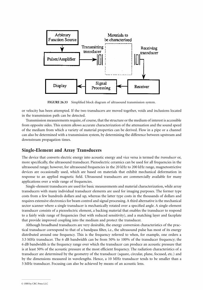
or velocity has been attempted. If the two transducers are moved together, voids and inclusions locatedin the transmission path can be detected.

Transmission measurements require, of course, that the structure or the medium of interest is accessiblefrom opposite sides. This system allows accurate characterization of the attenuation and the sound speedof the medium from which a variety of material properties can be derived. Flow in a pipe or a channelcan also be determined with a transmission system, by determining the difference between upstream anddownstream propagation times.

Single-Element and Array Transducers

The device that converts electric energy into acoustic energy and vice versa is termed the transducer or,more specifically, the ultrasound transducer. Piezoelectric ceramics can be used for all frequencies in theultrasound range; however, for ultrasound frequencies in the 20 kHz to 200 kHz range, magnetostrictivedevices are occasionally used, which are based on materials that exhibit mechanical deformation inresponse to an applied magnetic field. Ultrasound transducers are commercially available for manyapplications over a wide range of frequencies.

Single-element transducers are used for basic measurements and material characterization, while arraytransducers with many individual transducer elements are used for imaging purposes. The former typecosts from a few hundreds dollars and up, whereas the latter type costs in the thousands of dollars andrequires extensive electronics for beam control and signal processing. A third alternative is the mechanicalsector scanner where a single transducer is mechanically rotated over a specified angle. A single-elementtransducer consists of a piezoelectric element, a backing material that enables the transducer to respondto a fairly wide range of frequencies (but with reduced sensitivity), and a matching layer and faceplatethat provide improved coupling into the medium and protect the transducer.

Although broadband transducers are very desirable, the energy conversion characteristics of the prac-tical transducer correspond to that of a bandpass filter, i.e., the ultrasound pulse has most of its energydistributed around one frequency. This is the frequency referred to when, for example, one orders a3.5 MHz transducer. The 6 dB bandwidth can be from 50% to 100% of the transducer frequency; the6 dB bandwidth is the frequency range over which the transducer can produce an acoustic pressure thatis at least 50% of the acoustic pressure at the most efficient frequency. The radiation characteristics of atransducer are determined by the geometry of the transducer (square, circular, plane, focused, etc.) andby the dimensions measured in wavelengths. Hence, a 10 MHz transducer tends to be smaller than a5 MHz transducer. Focusing can also be achieved by means of an acoustic lens.

FIGURE 26.33 Simplified block diagram of ultrasound transmission system.


Array transducers exist in three main categories: phased arrays, linear arrays, and annular arrays. Afourth category could exist commercially in a few years: the 2-D array or a sparse 2-D array. Commonfor these array transducers is the fact that during transmission, the excitation time and excitation signalamplitude for each transducer element are controlled independently. This allows the beam to be steeredin a given direction, as well as focused at a given point in space. During reception, an independentlycontrolled time delay — which may be time varying — can be applied to each element before summationwith the signal from other elements. The delay control permits the transducer to have maximal sensitivityto an echo from a specified range, and, moreover, to shift this point in space away from the transduceras echoes from structures further away are received. A limitation of the phased and linear arrays is thatbeam steering and focusing can only take place within the image plane. In the direction normal to theimage plane, a fixed focus is produced by the physical shape of the array elements.

The phased array transducer consists of a fairly small number of elements, such as 16 to 32. Bothbeam steering and focusing are carried out, producing a pie-shaped image. The phased array is mostsuitable when only a narrow observation window exists, as is the case when imaging the heart from thespace between the ribs. The linear array transducer has far more elements, typically between 128 and256. It activates only a subset of all the elements for a given measurement, and produces focusing, butgenerally not beam steering, so that the beam direction is normal to the array surface. Consider a lineararray transducer with 128 elements, labeled 1 to 128. If one assumes that the first pulse-echo measurementis made with elements 1 to 16, the next measurement with elements 2 to 17, etc., the beam will havebeen linearly translated along the long dimension of the linear array (hence the name), producing arectangular image format. The annular array transducer consists of a series of concentric rings. As such,it cannot steer the beam, but can focus both in transmit and receive mode, just as the phased and lineararrays. Thus, the annular array transducer is not suitable for imaging unless the transducer is movedmechanically. Its specific advantage is uniform focusing.

Selection Criteria for Ultrasound Frequencies

The discussion so far has often mentioned frequency as an important variable, without providing anyguidance as to what ultrasound frequencies should be used. There is generally no technological limitationwith respect to choice of ultrasound frequency, as frequencies even in the gigahertz (GHz, 109 Hz) rangecan be produced. The higher the frequency, the better is the control over the direction and the width ofthe ultrasound beam, leading to improved axial and lateral resolution. However, the attenuation increaseswith higher frequency. For many media, the attenuation varies with the frequency squared; while forbiological soft tissue, the attenuation varies nearly linearly with frequency.

Generally, the ultrasound frequency is chosen as high as possible while still allowing a satisfactorysignal-to-noise ratio (SNR) of the received signal. This rule does not always hold; for example, for grainsize estimation in metals and for rough surface characterization, the optimal frequency has a specificrelationship to the mean grain dimension or the rms roughness.

Basic Parameters in Ultrasound Measurements

Ultrasound technology today has led to a very wide range of applications, and the following overviewmentions only the basic parameters. For an in-depth review, see [3]. A discussion of applications is givenat the end of the Ultrasound Theory and Applications section.

Reflection (or Transmission) Detected or Not

The most basic measurement consists of determining whether a reflected or transmitted signal is receivedor not. This can be used to monitor liquid level where the absence of liquid prevents ultrasoundtransmission from taking place, or to detect the existence of bubbles in a liquid (e.g., for dialysis purposes,where the bubbles are the reflectors) or for counting objects, such as bottles, on a conveyer belt.


Travel Time

Travel time is the elapsed time from transmission of an ultrasound pulse to the detection of a receivedpulse in either a pulse-echo or a transmission system. If the sound speed is known, the thickness of anobject can be found from the time difference between the front surface echo and the back surface echo.Conversely, sound speed can be determined when the thickness is known. By measuring with a broadbandpulse (a short pulse containing a broad range of frequencies), velocity dispersion (frequency dependenceof velocity) can be found, which has applications for materials characterization. Elastic parameters canalso be found from velocity measurements. Imaging applications are generally made based on theassumption of a known, constant velocity; thus, round-trip travel times from the transducer to thereflecting structures and back in a known direction gives the basis for the image formation.

Attenuation

The attenuation and its frequency dependence are important materials parameters, as they can be usedto differentiate between normal and pathological biological tissue, measure porosity of ceramics, thegrain size of metals, and the structure of composite materials. Attenuation can be found by means oftransmission measurements by determining the signal amplitude with the test object first absent andthen present; here, transmission losses must also be considered, as quantified in Equation 26.9. Attenu-ation can be obtained from pulse-echo measurements, by comparing the strength of echoes from thefront and back surfaces of the specimen under test. Diffraction effects (described later in the AdvancedTopics in Ultrasound section) might need to be considered. Attenuation can be considered as a bulkparameter for the medium as a whole, or it can be determined for small regions of the medium.

Reflection Coefficient

The strength of a reflection at an interface between two media is determined by the change in acousticimpedance across the interface, as shown in Equation 26.8. This allows, at least in principle, the impedanceof one medium to be determined from the measured reflection coefficient and the impedance of theother medium. In fact, the term impediography refers to the determination of the impedance profile ofa layered medium by means of this concept. In practice, the measurement is not easy to carry out, as thetransducer must be aligned very accurately at normal incidence to the medium surface. By measuringthe reflection coefficient vs. incident angle at a planar, smooth surface, a velocity estimate of the reflectingmedium can be made; in an alternative application, reflection measurements vs. frequency permit theevaluation of rough surface parameters.

Parameters Obtained Through Signal Processing

A number of object parameters can be obtained from analysis of the received signals. Material propertiescan be extracted from speckle analysis (analysis of statistical fluctuations in the image) and other formsof statistical analysis. Recognition of objects with complex shapes can, in some cases, be done by extractingspecific features of the received signals. Doppler processing for velocity estimation is another exampleof information that is only attainable by means of signal processing. By combining several “stacked”images, 3-D reconstruction is possible, from which volume estimation and rate of change of volume arepossible, such as for determining the dynamics of the left ventricle of the heart.

Ultrasound Theory and Applications

Sound Velocity

The propagation speed, c0, is generally determined by the density and the elastic properties of the medium.For an ideal gas, c0 may be expressed as [4]:

(26.10)c P rT0 0 0= =γ ρ γ K


where γ = CP/CV, the ratio of specific heats; for air, γ = 1.402. P0 is the static pressure of the gas, whichat 1 atm is 1.013 × 105 N m–2. ρ0 is the specific density of the gas, equal to 1.293 kg m–3 for air at 1 atmand 0°C. The constant r is the ratio of the universal gas constant and the molecular weight of the gas,and TK is the temperature in kelvin. Substituting the values for air into the first equation in Equation 26.10gives c0 = 331.6 m s–1 at 0°C. As the ratio P0/ρ0 is constant for varying pressure, but constant temperature,c0 is likewise pressure independent. (For a real gas, c0 exhibits, in fact, a small dependence on pressure.)

The temperature dependence of an ideal gas can be obtained by rewriting the second expression inEquation 26.10 as follows

(26.11)

where cref is the sound speed at 0°C, and T is the temperature in °C.In liquids, the expression for c0 is given as

(26.12)

where Ks is the adiabatic bulk modulus. Expressions for actual liquids as a function of temperature andpressure are not easily derived, and are often empirically determined. For pure water, the sound speedas a function of temperature and pressure can be given as:

(26.13)

In Equation 26.13, T is temperature in °C, and P0 is the static pressure in N m–2; the expression is validfor a pressure range from 1 atm to 100 atm.

Finally, for solids, the sound speed for longitudinal waves, cL, is [5]:

(26.14)

In Equation 26.14, cij is the the elastic stiffness constant, such that c11 refers to longitudinal stress overlongitudinal strain, and λ = c12 and µ = c44 are the Lamé elastic constants.

Wave Propagation in Homogeneous Media

In order to effectively use ultrasound for measurement purposes, it is essential to be able to describe thebehavior of acoustic fields. This includes the general behavior, and maybe even a detailed understanding,of the radiated field from ultrasound transducers; the transmission, reflection, and refraction of anacoustic field at boundaries and layers; and the diffraction of of acoustic field at finite-sized reflectors.

The wave equation is a differential equation that formulates how an acoustic disturbance (acousticpressure or particle velocity) propagates through a homogeneous medium. For an arbitrary wave field,the wave equation takes the following general form:

(26.15)

where ∇ 2 is the Laplacian operator. Equation 26.15 is also valid when particle velocity is substituted forpressure. If the condition of a plane wave field at a single frequency (also called a harmonic plane wavefield) is imposed, the solution to Equation 26.15 is:

(26.16)

c c T0 1 273= +ref

c K0 0= s ρ

c T T T PH O2= + − + + × −1402 4 5 01 0 055 0 00022 1 6 102 3 6

0. . . . .

cc

L =

= + µ

11

0

1 2

0

1 2

2

ρλ

ρ

∇ = ∂∂

2

2

2

2

1p

c

p

t

p t A j t B j tr r r r rr k r k r, exp exp( ) = − ×( )[ ] + + ×( )[ ]ω ω


In Equation 26.16, p(→r,t) consists of a plane wave propagating in the direction defined by the propa-gation vector

→k and a plane wave in the direction –

→k. As before, →r is a position vector that, in a Cartesian

coordinate system, can be expressed as →r = xx + yy + zz where x, y, and z are unit vectors. The magnitudeof

→k is called the wavenumber:

(26.17)

Expressing→k in the Cartesian coordinate system gives:

(26.18)

When k, kx, and ky are specified, kz is defined as well:

(26.19)

Applying the expressions for →r and→k to Equation 26.16 and considering only the plane wave in the

direction of +→k gives

(26.20)

From Equation 26.20, one sees that the amplitude of a plane wave is constant and equal to A, but thatthe phase varies with both time and space. When the direction of

→k is specified, kx, ky, and kz are found

from projection onto the coordinate axes.Solving Equation 26.15 under the assumption of spherical waves at a single frequency, with the source

placed at the origin of the coordinate system, gives:

(26.21)

The first term is a diverging spherical wave, and the second term is a converging spherical wave. Thereason that the vector dot product does not appear in Equation 26.21 is that

→k and →r always point in

the same direction for spherical waves. While Equation 26.21 gives the complete solution, in most casesonly a diverging spherical wave exists. If spherical waves are produced by a spherical source of radius a,then:

(26.22)

Acoustic Intensity and Sound Levels

The acoustic intensity, I, describes the mean power transported through a unit area normal to thedirection of propagation. A general expression for I for a CW pressure function is:

(26.23)

k c= = πω λ0 2

rk = + +k x k y k zx y z

ˆ ˆ ˆ

k c k kz x2

y2= ( ) − −

ω 0

2

p t A j t k x k y k zrr, exp( ) = − + +( )( )

ω x y z

p r tA

rj t kr

B

rj t kr, exp exp( ) = −( )[ ]+ +( )[ ]ω ω

p r tA

rj t kr r a, exp , ( ) = −( )[ ] >ω

IT

p t u t dt

T

= ( ) ( )∫1

0


In Equation 26.23, T represents one full cycle of the pressure function, and u(t) is the particle velocityfunction. For a plane wave, the intensity is:

(26.24)

where P and U are the magnitudes of the pressure and the particle velocity functions, respectively. Theexpression for I in Equation 26.24 can also be used as an approximation for nonplanar waves, such asspherical waves, as long as (kr) is large.

The intensity levels for pulse-echo measurements are often described by the SPTA (Spatial Peak, TemporalAverage) value, which therefore refers to the mean intensity at the point in space where the intensity is thehighest. Although the guidelines for exposure levels for medical imaging, set by the FDA, vary for differentparts of the body, a general upper limit is 100 mW cm–2. Given that the duty cycle (pulse duration/pulseinterval) is typically in the order of 0.0001 for ultrasound imaging, the temporal peak intensity is muchhigher, and is even approaching the level where nonlinear effects can begin to be observed. Intensity levelsused for NDE are application dependent, but are generally in the same range as in medical ultrasound.

Sound levels are logarithmic expressions (expressions in dB) of the pressure level or the intensity level.The term SPL stands for sound pressure level and is given as:

(26.25)

In Equation 26.25, Pe is the effective pressure of the acoustic wave and Pref is the reference effectivepressure. Correspondingly, IL is the intensity level defined as:

(26.26)

where Iref is the reference acoustic intensity.Several reference levels are commonly used [6]. In air, Pref = 20 µPa and Iref = 10–12 W m–2 are nearly

equivalent reference levels. For water, typical pressure reference levels are Pref = 1 µPa, Pref = 20 µPa orPref = 1 µbar = 0.1 Pa, with corresponding intensity reference levels of Iref = 6.76 × 10–19 W m–2, Iref = 2.70 ×10–16 W m–2, and Iref = 6.76 × 10–9 W m–2.

Wave Propagation Across Layers and Boundaries

The reflection and transmission coefficients for a plane wave impinging at normal incidence on theinterface between two half spaces were given in Equations 26.8 and 26.9. It is also important to considerthe transmission and reflection of waves at non-normal incidence and across a layer.

When a longitudinal wave impinges at a liquid–liquid interface, both the transmitted and the reflectedwaves are longitudinal waves, as illustrated in Figure 26.34(a). However, when a longitudinal wavepropagating in a liquid medium encounters a liquid–solid interface under oblique incidence, both alongitudinal and a shear transmitted wave and a longitudinal reflected wave will result, as shown inFigure 26.34(b). The change of direction of the transmitted waves relative to the incident wave is referredto as refraction, which is caused by the difference in sound speed between the two media.

The magnitude and direction of the reflected and transmitted waves are determined by two simpleboundary conditions: (1) the pressure on both sides of the boundary must be equal at all times, and(2) the normal particle velocity on both sides of the boundary must be equal at all times; the normalparticle velocity refers to the component of the particle velocity that is normal to the boundary.

The boundary conditions lead to the following two relationships:

(26.27)

IP

cPU= =

2

0 02

1

2ρ

SPL dBe ref= ( ) [ ]20log P P

IL dBref= ( ) [ ]10 log I I

sin sin ; sin sinθ θ θ θ

i ri t= =

c c1 2


where c1 and c2 are the sound speeds of the two media, and θi, θr, and θt are the incident, reflected andtransmitted angles, respectively. From Equation 26.27, one sees that

(26.28)

The second expression in Equation 26.28 is referred to as Snell’s law and quantifies the degree of refraction.Refraction affects the quality of ultrasound imaging because image formation is based on the assumptionthat the ultrasound beam travels in a straight path through all layers and inhomogeneities, and that thesound speed is constant throughout the medium. When the actual beam travels along a path that deviatesto some extent from a straight path and passes through some parts of the medium faster than it doesother parts, the resulting image is a distorted depiction of reality. Correcting this distortion is a verycomplex problem and, in the near future, one should only expect image improvement in the simplest cases.

It can be seen from Equation 26.28 that angle θt is not defined if the argument to the arcsin functionexceeds unity. This defines a critical incident angle as follows:

(26.29)

at or above which the reflection coefficient is 1 and the transmission coefficient is 0. A critical angle onlyexists when c1 < c2. The transmitted shear and longitudinal velocities each correspond to a differentcritical angle of incidence.

From the boundary conditions, the reflection coefficient as a function of incident angle can bedetermined [7]:

FIGURE 26.34 (a). An incident longitudinal wave at a liquid–liquid interface produces a reflected and a transmittedlongitudinal wave. (b) An incident longitudinal wave at a liquid–solid interface produces a reflected longitudinalwave, transmitted longitudinal, and shear waves. The incident, reflected, and transmitted angles are indicated.

θ θ θ θr i t i= =

; arcsin sin

c

c2

1

sinθc = c

c1

2


(26.30)

The result in Equation 26.30 is referred to as the Rayleigh reflection coefficient.The transmission of plane waves under normal incidence through a single layer is often of interest.

The dimensions and the medium parameters are defined in Figure 26.35.By applying the boundary conditions to both interfaces of the layer, both reflection and transmission

coefficients are obtained [7], as given in Equations 26.31 and 26.32.

(26.31)

(26.32)

A number of special conditions for Equation 26.31 can be considered, such as: (1) z1 = z3, which simplifiesthe numerator in Equation 26.31; and (2) the layer thickness is only a small fraction of a wavelength,that is, k2L « 1 which makes cos k2L ≈ 1 and sin k2L ≈ k2L. One case is of particular interest: the choiceof thickness and acoustic impedance for the layer that makes R = 0, and therefore gives 100% energytransmission. This is fulfilled for:

(26.33)

The result in Equation 26.33 states that the layer must be a quarter of a wavelength thick (plus an integernumber of half wavelengths) and must have an acoustic impedance that is the geometric mean of theimpedances of the media on either side. Among several applications of the quarter wavelength impedancematching is the impedance matching between a transducer and the medium, such as water. A drawbackwith a single matching layer is that it only works effectively over a narrow frequency range, while the

FIGURE 26.35 A pressure wave is incident on a layer of thickness L and with acoustic impedance z2 = ρ2 c2.

Rz z

z zc cθ

θ θ

θ θθ θi

t i

t i

t iwhere( ) =( ) − ( )( ) + ( ) = − ( )2 1

2 1

2 1

221

cos cos

cos cos, cos sin

Rp

p

z z k L j z z z z k L

z z k L j z z z z k L= =

−( ) + −( )+( ) + +( )

r

i

1

1

1 3 2 2 3 1 2 2

1 3 2 2 3 1 2 2

cos sin

cos sin

Tp

p z z k L j z z z z k L= =

+( ) + +( )t

i

2

1 1 3 2 2 3 1 2 2cos sin

k L n z z z2 2 1 32= π + π =;


actual acoustic pulse contains a fairly broad spectrum of frequencies. A better matching is achieved byusing more than one matching layer, and it has been shown that a matching layer that has a continuouslyvarying acoustic impedance across the layer provides broadband impedance matching.

Attenuation: Its Origin, Measurement, and Applications

Attenuation refers to the damping of a signal, here specifically an acoustic signal, with travel time or withtravel distance. Attenuation is typically expressed in dB, i.e., on a logarithmic scale. Attenuation is animportant parameter to measure in many types of materials characterization, but also the parameter thatsets an upper limit for the ultrasound frequency that can be used for a given measurement. In NDE,attenuation is used for grain size estimation [8, 9], for characterization of composite materials, and fordetermination of porosity [10]. In medical ultrasound, attenuation can be used for tissue characterization[11], such as differentiating between normal and cirrhotic liver tissue and for classification of malignan-cies. In flowmeters, attenuation caused by vortices can be used to measure the frequency at which theyare shed; this frequency is proportional to the flow velocity.

Attenuation represents the combined effect of absorption and scattering, where absorption refers tothe conversion of acoustic energy into heat due to the viscosity of the medium, and scattering refers tothe spreading of acoustic energy into other directions due to inhomogeneities in the medium. Theabsorption can, in part, be due to classical absorption, which varies with frequency squared, and relaxationabsorption, which can result in a complicated frequency dependence of absorption. Gases (except fornoble gases), liquids, and biological tissue exhibit mainly relaxation absorption, whereas classical absorp-tion is most prominent in solids, which can also have a significant amount of scattering attenuation.

In general, absorption dominates in homogeneous media (e.g., liquids, gases, fine-grained metals,polymers), whereas scattering dominates in heterogeneous media (e.g., composites, porous ceramics,large-grained materials, bone). The actual attenuation and its frequency dependence can be specifiedfairly unambiguously for gases and liquids, while for solids it is very dependent on the manufacturingprocess, which determines the microstructure of the material, such as the grain structure.

Measurement of attenuation can be carried out for at least two purposes: (1) to measure the bulkattenuation of a given homogeneous medium; and (2) to measure the spatial distribution of attenuationover a plane in an inhomogeneous medium. The former approach is most common in materials char-acterization, whereas the latter approach is found mainly in medical ultrasound. Bulk attenuation canbe performed either with transmission measurements or with pulse-echo measurements, as illustratedin Figure 26.36(a) and (b), respectively.

For the measurement of attenuation, in dB/cm, of a medium of thickness d, by transmission measure-ments, define v1(t) as the received signal without medium present and v2(t) as the received signal withmedium present, as shown in Figure 26.36(a). The attenuation is then determined from the ratio of theenergies of the two signals, corrected for the transmission losses, as:

(26.34)

Correction for transmission losses (2nd term) can be avoided by alternatively measuring the incrementalattenuation due to an incremental thickness increase.

For the measurement of attenuation by pulse-echo measurements, the front and the back wall echoesare termed vf(t) and vb(t), respectively. Based on an a priori knowledge of the pulse duration, a timewindow ∆T is defined. The attenuation is most accurately measured when based on the energies of vf(t)and vb(t), but may alternatively be based on the amplitudes of vf(t) and vb(t), as stated in Equation 26.35.

Att dB cm[ ] =( )[ ]( )[ ]

−+( )

∞

∞

∫

∫1

10 204

1

2

0

2

2

0

1 2

1 2

2d

v t dt

v t dt

z z

z zlog log


(26.35)

Accurate attenuation measurements require attention to several potential pitfalls: (1) diffraction effects(even in the absence of attenuation, echoes from different ranges vary in amplitude, due to beamspreading); (2) misalignment effects (if the reflecting surface is not normal to the transducer axis, thereis a reduction in detected signal amplitude, due to phase cancellation at the transducer surface); and(3) transmission losses whose magnitude it is not always easy to determine.

The spatial distribution of attenuation must be measured with pulse-echo measurements, where it isassumed that a backscatter signal of sufficient amplitude can be received from all regions of the medium.Use is made of the frequency dependence of attenuation, which has the effect that the shift in meanfrequency of a given received echo relative to the mean frequency of the transmitted signal variesproportional to the total absorption. The rate of shift in mean frequency is thus proportional to the localattenuation.

CW Fields from Planar Piston Sources

In discussing the acoustic fields generated by acoustic radiators (transducers), a clear distinction mustbe made between fields due to CW excitation and due to pulse excitation. Although the overall field

FIGURE 26.36 Measurement of bulk attenuation. (a) Measurement of attenuation by transmission measurement.(b) Measurement of attenuation by pulse-echo measurements.

Att dB cmpeak ampl.,

peak ampl.,

f

b

f

b

[ ] =( )[ ]( )[ ]

≅( )( )

∫

∫1

210

1

220

2

0

2

0

d

v t dt

v t dtd

v t

v t

t

Tlog log

∆

∆


patterns for these two cases are quite similar, the detailed field structure is very different. In this section,only CW fields are discussed.

When a CW excitation voltage is applied to a planar piston transducer, the resulting acoustic field canbe divided into a near field region and a far field region. This division is particularly distinct when thetransducer has a circular geometry. A piston transducer simply refers to a transducer with the samevelocity amplitude at all points on the surface. The length of the near field, NF, is given as:

(26.36)

where a is the radius of the transducer and λ is the wavelength. As shown in Figure 26.37(a), the nearfield is approximately confined while the far field is diverging. The angle of divergence, θ, is approximately:

(26.37)

Additional comments to the simplified representation in Figure 26.37(a) are in order:

1. The actual field has no sharp boundaries, in contrast to what is shown in Figure 26.37.2. While the beam diameter is roughly constant in the near field, it is not as regular as shown; and

at the same time, the near field structure is very complex.3. The angle of divergence, θ, is only clearly established well into the far field.4. The depiction of the far field shows only the main lobe; in addition, there are side lobes, which

are directions of significant pressure amplitude, separated by nulls (i.e., directions with zeropressure amplitude).

FIGURE 26.37 Pressure fields from a circular planar piston transducer operating with CW excitation. NF = NearField. (a) Approximate field distribution in near field and far field. (b) Axial pressure in near field and far field for(ka) = 31.4.

NF = a2

λ

θ λ=

arcsin .0 61

a


In general, analytical expressions do not exist for the pressure magnitude at an arbitrary field pointin the near field, and the pressure must instead be calculated by numerical techniques. However, an exactexpression exists for the axial pressure amplitude, Pax, valid in both near and far field [12].

(26.38)

In Equation 26.38, U0 is the amplitude of the velocity function on the surface of the transducer. Theexpression is derived for a baffled planar piston transducer where the term “baffled” means that thetransducer is mounted in a large rigid surface, called a baffle. Figure 26.37(b) shows the amplitude ofthe axial field for a planar piston transducer for which (ka) = 31.4. For field points located more than3 to 4 near-field distances away from the transducer, a general expression for the pressure amplitude canbe derived [12]:

(26.39)

where J1(·) is the Bessel function of the first order. The variable r is the length of the position vectordefining the field point, and angle θ is the angle that the position vector makes with the x-axis.

Of interest in evaluating transducers in the far field is the directivity, D, defined as follows:

(26.40)

Thus, the directivity gives the factor with which the axial intensity of the given source is increased overthat of a simple source (omnidirectional radiator), radiating the same total energy. For a baffled, circularplanar piston transducer, the directivity in the far field can be calculated to be [12]:

(26.41)

When (2ka) » 1, Equation 26.41 can be approximated to D = (ka)2. Directivity values in the 1000s arecommon. For example, a 3.5 MHz transducer with 1 cm diameter radiating into water has a (ka) valueof 73.3 and a directivity of 5373.

Often, focused transducers are used where the focusing is either created by the curvature of thepiezoelectric element or by an acoustic lens in front of the transducer. The degree of focusing is deter-mined by the (ka) value of the transducer.

Generation of Ultrasound: Piezoelectric and Magnetostrictive Phenomena

Ultrasound transducers today are available over a wide frequency range, in many sizes and shapes, andfor a wide variety of applications. The behavior of the ultrasound transducer is determined by severalparameters: the transduction material, the backing material, the matching layer(s), and the geometryand dimension of the transducer. A good overview of ultrasound transducers is available in [13].

The transduction material is most commonly a piezoelectric material, but can for some applicationsbe a magnetostrictive material instead. These materials are inherently narrowband, meaning that theywork efficiently only over a narrow frequency range. This is advantageous for CW applications such as

P x c U ka x a x aax( ) = + − ( )

2 0 5 10 0 0

2 2ρ sin .

P rc

U kaa

r

J ka

ka,

sin

sinθ ρ θ

θ( ) =

( )

0 00

1

2

2

D xI x

I x( ) =

( ) [ ]( ) [ ]

ax

ax

given source

simple source

Dka

ka J ka=

( )− ( )

3

1 2


ultrasound welding and ultrasound hyperthermia, but is a problem for imaging applications, as impulseexcitation will produce a long pulse with poor resolving abilities. To overcome this deficiency, a backingmaterial is tightly coupled to the back side of the transducer for the purpose of damping the transducerand shortening the pulse. However, the backing material also reduces the sensitivity of the transducer.Some of this reduced sensitivity can be regained by the use of a matching layer, specifically selected forthe medium of interest. As seen in Equation 26.33, a quarter wavelength matching layer can provide100% efficient coupling to a medium, albeit only at one frequency. A combination of several matchinglayers can provide a more broadband impedance matching. The field is determined by both the geometry(planar, focused, etc.) of the transducer and by the frequency content of the velocity function of thesurface of the transducer. In this section, unique aspects of the transduction material itself are described.

Piezoelectric Materials.A piezoelectric material exhibits a mechanical strain (relative deformation) due to the presence of anelectric field, and generates an electric field when subjected to a mechanical stress. A detailed review ofpiezoelectricity is given in [14]. Piezoelectric materials can either be: (1) natural material such as quartz;(2) man-made ceramics (e.g., barium titanate (BaTi), lead zirconate titanate (PZT), or lead meta-niobate);(3) man-made polymers (e.g., polyvinylidene fluoride (PVDF)). The piezoelectric ceramics are the mostcommonly used materials for ultrasound transducers. These ceramics are made piezoelectric by a so-called poling process in which the material is subjected to a strong electric field while at the same heatingit to above the material’s Curie temperature.

Several material constants determine the behavior of a given piezoelectric material, the most importantof which are listed in Table 26.3 and defined below. An extensive list of parameter values for variouspiezoelectric materials is available in [15].

d33 Transmission constantg33 Receiving constantk33 Piezoelectric coupling coefficientkT Piezoelectric coupling coefficient for a transverse clamped materialQM Mechanical Q

The transmission constant, d33, gives the mechanical deformation of piezoelectric materials for fre-quencies well below the resonance frequency. A transducer with a large d33 value will therefore becomean efficient transmitter. If an electric field, E3, is applied in the polarized direction of a piezoelectric rodor disk, the strain, S3, in that direction is approximately:

(26.42)

where Vappl is the applied voltage and l is the thickness. The total deformation, ∆ l, becomes

(26.43)

TABLE 26.3 List of Most Significant Piezoelectric Parameters for Common Piezoelectric Materials

ParameterBarium titanate Lead zirconate Lead meta-niobate, Polyvinylidene

(BaTiO3) titanate, PZT-5 PbNb2O6 fluoride (PVDF)

d33 149 (10–12 m/V) 374 (10–12 m/V) 75 (10–12 m/V) 22 (10–12 m/V)g33 14 (10–3 Vm/N) 25 (10–3 Vm/N) 35 (10–3 Vm/N) 339 (10–3 Vm/N)k33 0.50 0.70 0.38 k31 = 0.12kT 0.38 0.68 0.40 0.11Qm 600 75 5 19

S d E dV

l3 33 3 33= = appl

∆l d V= 33 appl


The receiving constant, g33, defines the sensitivity of a transducer element as a receiver when the frequencyof the applied pressure is well below the resonance frequency of the transducer. If the applied stress(force/area) in the direction of polarization is T3, the output voltage from a rod or disk is approximately:

(26.44)

The coupling coefficient describes the power conversion efficiency of a piezoelectric transducer, oper-ating at or near resonance. Specifically, k33 is the coupling coefficient for an unclamped rod; that is, therod is allowed to deform in the directions orthogonal to the direction of applied force or voltage. Incontrast, kT is the coupling coefficient for a clamped disk. Finally, QM gives the mechanical Q, which isa measure for how narrowband the transducer material inherently is.

Whereas expressions of the type given in Equations 26.42 to 26.44 are adequate for describing staticor low-frequency behavior, the behavior near resonance where most transducers operate requires morecomplex models, which are beyond the scope of this chapter. The Mason model is adequate for narrow-band modeling of transducers, whereas the KLM or Redwood models better describe the transducers forbroadband applications [13, 15].

Magnetostrictive Materials.The magnetostrictive phenomenon refers to a magnetically induced contraction or expansion in ferro-electric media, such as in nickel or alfenol, and was discovered by Joule in 1847. Magnetostrictive materialsare generally used for ultrasound frequencies below 100 kHz, and are therefore relevant mainly forunderwater applications. Eddy current losses influence the performance of magnetostrictive materials,but the losses can be reduced by constructing the magnetostrictive transducer from thin laminations.

Transducer Specifications.Ultrasound transducers are generally specified by their diameter, center frequency, focal distance, andtype of focusing (if applicable). The transducer can be designed as a contact transducer, a submersibletransducer, an air transducer, etc.; in addition, the type of connector or cabling can be specified. In manycases, measurement data for the actual transducer can be supplied by the vendor in the form of a measuredpressure pulse and the corresponding frequency spectrum, recorded with a hydrophone at a specific fieldpoint. Similarly, the beam profile can be measured in the form of pulse amplitude or pulse energy as afunction of lateral position.

Detailed information about the acoustic field from a radiating transducer can be obtained with eitherthe Schlieren technique or the optical interferometric technique. Such instruments are quite expensive,falling in the $50K to $120K range.

Display Formats for Pulse-Echo Measurements

The basic description of ultrasound imaging was presented earlier in this chapter. Based on the infor-mation presented so far in this section, more specific aspects of pulse-echo ultrasound imaging will nowbe described. Different display formats are used; the simplest of these is the A-mode display.

A-mode.When a pulse-echo transducer has emitted a pulse in a given direction and has been switched to receivemode, an output signal from the transducer is produced based on detected echoes from different ranges,as illustrated conceptually in Figure 26.31(a). In this signal, distance to the reflecting structure has beenconverted into time from the start of signal. This signal is often referred to as the RF signal. Demodulatingthis signal (i.e., generating the envelope of the signal) produces the A-mode (amplitude mode) display,or the A-line signal. This signal can be the basis for range measurements, attenuation measurements,and measurement of reflection coefficient.

M-mode.If the A-mode signal from a transducer in a fixed position is used to intensity modulate a cathode-raytube (CRT), such as a monitor or oscilloscope, along a straight vertical line, a line of dots with brightness

v g T lout = 33 3


according to echo strengths would appear on the screen. Moving the display electronically across thescreen results in a set of straight horizontal lines. Now consider the case where the reflecting structuresare moving in a direction toward or away from the transducer while pulse-echo measurements werebeing performed. This results in variations in the arrival time of echoes in the A-line signal, and theresulting lines across the screen are no longer straight, but curved, as determined by their velocity. Sucha display is called M-mode, or motion mode, display. An application for this would be measurement ofthe diameter variation of a flexible tube, or blood vessel, due to a varying pressure inside the tube.

B-mode.If pulse-echo measurements are repeatedly being performed, while the transducer scans the object ofinterest, an image of the object can be generated, as illustrated in Figure 26.31. Specifically, each A-linesignal is used to intensity modulate a line on a CRT corresponding to the location of ultrasound beam,which produces an image that maps the reflectivity of the structures in the object. The resulting imageis called a B-mode (or brightness mode) image. If the transducer is moved linearly, a rectangular imageis produced, whereas a rotated transducer generates a pie-shaped, or sector image. This motion is typicallydone electronically or electromechanically, as described earlier under single-element and array transduc-ers. When the scanning is done rapidly (say, 30 scans/s), the result is a real-time image.

Many forms of signal processing and image enhancement can be applied in the process of generatingthe B-mode image. Echoes from deeper lying structures will generally be of smaller amplitude, due tothe attenuation of the overlying layers of the medium. Attenuation correction is made especially in medicalimaging, so that echoes are displayed approximately with their true strength. This correction consists ofa time-varying gain, called time-gain control, or TGC, such that the early arriving echoes experience onlya low gain and later echoes from deeper lying structures experience a much higher gain. Various formsfor signal compressions or nonlinear signal transfer function can selectively enhance the weaker or thestronger echoes.

C-mode.In a C-mode display, only echoes from a specific depth will be imaged. To generate a complete image,the transducer must therefore be moved in a raster scan fashion over a plane. C-scan imaging is slowand cannot be used for real-time imaging, but has several applications in NDE for examining a givenlayer, or interface, in a composite structure, or the inner surface of a pipe.

Flow Measurements by Doppler Signal Processing

Flow velocity can be obtained by various ultrasonic methods (Chapter 28, Section 7), e.g., by measuringthe Doppler frequency or Doppler spectrum. The Doppler frequency is the difference between thefrequency (or pitch) of a moving sound source, as measured by a stationary observer, and the actualfrequency of the sound source. The change in frequency is determined by the speed and direction of themoving source. The classical example is a moving locomotive with its whistle blowing; the pitch isincreased when the train moves toward the observer, and vice versa. With respect to ultrasound mea-surements, only the reflecting (or scattering) gas, fluid, or structure is moving and not the the soundsource, yet the Doppler phenomenon is present here as well. In order for ultrasound Doppler to function,the gas or fluid must contain scatterers that can reflect some of the ultrasound energy back to the receiver.The Doppler frequency, fd, is given as follows:

(26.45)

where v is the velocity of the moving scatterers, and θ is the angle between the velocity vector and thedirection of the ultrasound beam. Doppler flowmeters require only access to the moving gas, fluid, orobject from one side. For industrial use, when the fluids or gases often do not contain scatterers,transmission methods are preferred; these methods, however, are not based on the Doppler principle(Chapter 28, Section 7).

fv

cd = 2

0

cos θ


Two main categories of Doppler systems exist: the CW Doppler system and the PW (pulsed wave)Doppler system. The CW Doppler system transmits a continuous signal and does not detect the distanceto the moving structure. It is therefore only applicable when there is just one moving structure or clusterof scatterers in the acoustic field. For example, a CW Doppler is appropriate for assessing the pulsatilityand nature of blood flow in an arm or leg. CW Doppler systems are small and relatively inexpensive.

The PW Doppler system transmits a short burst at precise time intervals; it is therefore inherently asampled system, and, as such, is subject to aliasing. It measures changes from one transmitted pulse tothe next in the received signal from moving structures at one or several selected ranges, and is able todetermine both velocity and range. Assuming that the ultrasound beam is narrow and thus very direc-tional, the PW Doppler can create a flow image; that is, it can indicate the magnitude and direction offlow over an image plane. Commonly, color and color saturation are used to indicate direction and speedin a flow image, respectively. In contrast to CW Doppler systems, the PW Doppler systems require muchsignal processing and are therefore typically expensive and often part of a complete imaging system. Whena distribution of velocities, rather than a single velocity, is encountered, as is often the case with fluid flow,a Doppler spectrum rather than a Doppler frequency is determined. An FFT (Fast Fourier Transform)routine is then used to reveal the Doppler frequencies and thus the velocity components present.

Review of Common Applications of Ultrasound and Their Instrumentation

Range Measurements, Air

Ultrasound range measurements are used in cameras, in robotics, for determining dimensions of rooms,etc. Measurement frequencies are typically around 50 kHz to 60 kHz. The measurement concept is pulse-echo, but with burst excitation rather than pulse excitation. Special electronic circuitry and a thin low-acoustic-impedance air transducer is most commonly used. Rugged solid or composite piezoelectric-based transducers, however, can also be used, sometimes up to about 500 kHz.

Thickness Measurement for Testing, Process Control, Etc.

Measurement of thickness is a widely used application of ultrasound. The measurements can be donewith direct coupling between the transducer and the object of interest, or — if good surface contact isdifficult to establish — with a liquid or another coupling agent between the transducer and the object.Ultrasound measurements of thickness have applications in process control, quality control, measuringbuild-up of ice on an aircraft wing, detecting wall thickness in pipes, as well as medical applications. Theinstrumentation involves a broadband transducer, pulser-receiver, and display or, alternatively, echodetecting circuitry and numerical display.

Detection of Defects, such as Flaws, Voids, and Debonds

The main ultrasound application in NDE is inspection for the localization of voids, crack, flaws, deb-onding, etc. [3]. Such defects can exist immediately after manufacturing, or were formed due to stresses,corrosion, etc. Various types of standard or specialized flaw detection equipment are available fromultrasound NDE vendors.

Doppler Flow Measurements

The flow velocity of a liquid or a moving surface can be determined through Doppler measurements,provided that the liquid or the surface scatters ultrasound back in the direction of the transducer, andthat the angle between the flow direction and the ultrasound beam is known. Further details are givenin the section about Doppler processing. CW and PW Doppler instruments are commercially available,with CW instrumentation being by far the least expensive.

Upstream/Downstream Volume Flow Measurements

When flow velocity is measured in a pipe with access to one or both sides, an ultrasound transmissiontechnique can be used in which transducers are placed on the same or opposite sides of the pipe, with


one transducer placed further upstream than the other transducer. From the measured difference in traveltime between the upstream direction and the downstream direction, and knowledge about the pipegeometry, the volume flow can be determined. Special clamp-on transducers and instrumentation areavailable. An overview of flow applications in NDE is given in [16].

Elastic Properties of Solids

Since bulk sound speed varies with the elastic stiffness of the object, as given in Equation 26.15, soundspeed measurements can be used to estimate elastic properties of solids under different load conditionsand during solidification processes. Such measurements can also be used for measurement of productuniformity and for quality assurance. The measurements can be performed on bulk specimens or onthin rods, using either pulse-echo or transmission instrumentation [17]. Alternatively, measurements ofthe material’s own resonance frequencies can be performed for which commercial instruments, such asthe Grindo-sonics, are available.

Porosity, Grain Size Estimation

Measurement of ultrasound attenuation can reveal several materials parameters. By observing the atten-uation in metals as a function of frequency, the grain size and grain size distribution can be estimated.Attenuation has been used for estimating porosity in composites. In medical ultrasound, attenuation iswidely used for tissue characterization, that is, for differentiating between normal and pathological tissues.Pulse-echo instrumentation interfaced with a digitizer and a computer for data analysis is required.

Acoustic Microscopy

The measurement approaches utilized in acoustic microscopy are similar to other ultrasound techniques,in that A-scan, B-scan, and C-scan formats are used. It is in the applications and the frequency rangeswhere acoustic microscopy differs from conventional pulse-echo techniques. Although acoustic micro-scopes have been made with transducer frequencies up to 1 GHz, the typical frequency range is 20 MHzto 100 MHz, giving spatial resolutions in the range from 100 µm to 25 µm. Acoustic microscopy is usedfor component failure analysis, electronic component packaging, and internal delaminations and dis-bonds in materials, and several types of acoustic microscopes are commercially available.

Medical Ultrasound

Medical imaging is a large and diverse application area of ultrasound, especially in obstetrics, cardiology,vascular studies, and for detecting lesions and abnormalities in organs. The display format is either B-mode,using gray scale image, or a combination of Doppler and B-mode, with flow presented in color and stationarystructures in gray scale. A wide variety of instruments and scanners for medical ultrasound are available.

Selected Manufacturers of Ultrasound Products

Table 26.4 contains a representative list of ultrasound equipment and manufacturers.

Advanced Topics in Ultrasound

Overview of Diffraction

The ultrasound theory presented thus far has emphasized basic concepts, and the applications that havebeen discussed tacitly assume that the field from the transducer is a plane wave field. This simplifyingassumption is acceptable for applications such as basic imaging and measurements based on travel time.However, the plane wave assumption introduces errors when materials parameters (e.g., attenuation,surface roughness, and object shape) are sought to be measured with ultrasound. Therefore, to useultrasound as a quantitative tool, an understanding is needed of the structure of the radiated acousticfield from a given transducer with a given excitation, and — equally important — the ability to calculatethe actual radiated field. This leads to the topic of diffraction, which is the effect that accounts for thecomplex structure of both radiated and scattered fields. Not surprisingly, there are direct parallels betweenoptical diffraction and acoustic diffraction. (As a separate issue, it should be noted that the ultrasound


theory presented here assumes that the wave amplitudes [pressure, displacement] are small enough sothat nonlinear effects can be disregarded.)

Diffraction is basically an edge effect. Whereas a plane wave incident on a large planar interface isreflected in a specific direction, the plane wave incident on an edge results in waves scattered in manydirections. Similar considerations hold for the field produced by a transducer: The surface of the trans-ducer produces a so-called geometric wave that has the shape of the transducer itself; the edge of thetransducer, however, generates an edge wave with the shape of an expanding torus. The actual pressurefield is a combination of the two wave fields. Very close to a large transducer, the geometric wavedominates, and diffraction effects might not need to be considered. Over small regions far away fromthe transducer, the field can be approximated by a plane wave field, and diffraction does not need to beconsidered. However, in many practical cases, diffraction must be considered if detailed informationabout the pressure field is desired, and numerical methods must be employed for the calculations.

The structure of the axial field, shown in Figure 26.37(b), is a direct result of diffraction. Numericalevaluation of the diffracted field from a transducer can be done in several ways: (1) use of the Fresnelor Fraunhofer integrals (not applicable close to the transducer) to calculate the field at a single frequencyat a specified plane normal to the transducer axis; (2) calculation of the pressure function at any pointof interest in space, based on a specified velocity function, u(t), on the surface of the transducer, usingRayleigh integral; (3) decomposing the velocity field in the plane of the transducer into its plane wavecomponents, using a 2-D Fourier transform technique, followed by a forward propagation of the planewaves to the plane of interest and an inverse Fourier transform to give the diffracted field; or (4) use offinite element methods to calculate the diffracted field at any point or plane of interest. In the following,methods (1) and (2) will be described.

Fresnel and Fraunhofer Diffraction.Let the velocity function on the surface of the transducer, u(x,y), be specified for a particular frequency, ω.Assume that the transducer is located in the (x,y,0) plane and that one is interested in the pressure fieldin the (x0,y0,z) plane. The Fresnel diffraction formulation [18] assumes that the paraxial approximationis fulfilled, requiring z to be at least 5 times greater than the transducer radius, in which case the Fresneldiffraction integral applies:

(26.46)

TABLE 26.4 List of Products for and Manufacturers of Ultrasound Measurements

Product type Manufacturer

Ultrasound transducers Panametrics, 221 Crescent St., Waltham, MA 02154. (800) 225-8330Ultrasound transducers Krautkramer Branson Inc., 50 Industrial Park Rd., Lewistown, PA 17044. (717) 242-0327Range measurements, air Polaroid Corporation, Ultrasonics Components Group, 119 Windsor Street, Cambridge,

MA 02139. (800) 225-1618Pulser-receivers Panametrics, 221 Crescent St., Waltham, MA 02154. (800) 225-8330Pulser-receivers JSR Ultrasonics, 3800 Monroe Ave., Pittsfield, NY 14534. (716) 264-0480Ultrasound power ampl. Amplifier Research, 160 School House Rd., Souderton, PA 18964. (800) 254-2677Ultrasound power ampl. Ritec, 60 Alhambra Rd., Suite 5, Warwick, RI 02886. (401) 738-3660NDE instrumentation Panametrics, 221 Crescent St., Waltham, MA 02154. (800) 225-8330NDE instrumentation Krautkramer Branson Inc., 50 Industrial Park Rd., Lewistown, PA 17044. (717) 242-0327Acoustic microscopy Sonoscan, 530 E. Green St., Bensenville, IL 60106. (708) 766-4603Medical Imaging Hewlett Packard, Andover, MA; ATL, Bothell, WA; Diasonics, Milpitas, CA; Siemens

Ultrasound, Issaquah, WA.Schlieren based imaging

of acoustic fieldsOptison, 568 Weddell Drive, Suite 6, Sunnyvale, CA 94089. (408) 745-0383

Optical based imaging of acoustic fields

UltraOptec, 27 de Lauzon, Boucherville, Quebec, Canada J4B 1E7. (514) 449-2096

p x y zA

u x y jkx y

zjk

x x y y

zdx dy

z S0 0

02 2

0 0

2, , , , , exp expω

λω( ) = ( ) − +

+

∫∫


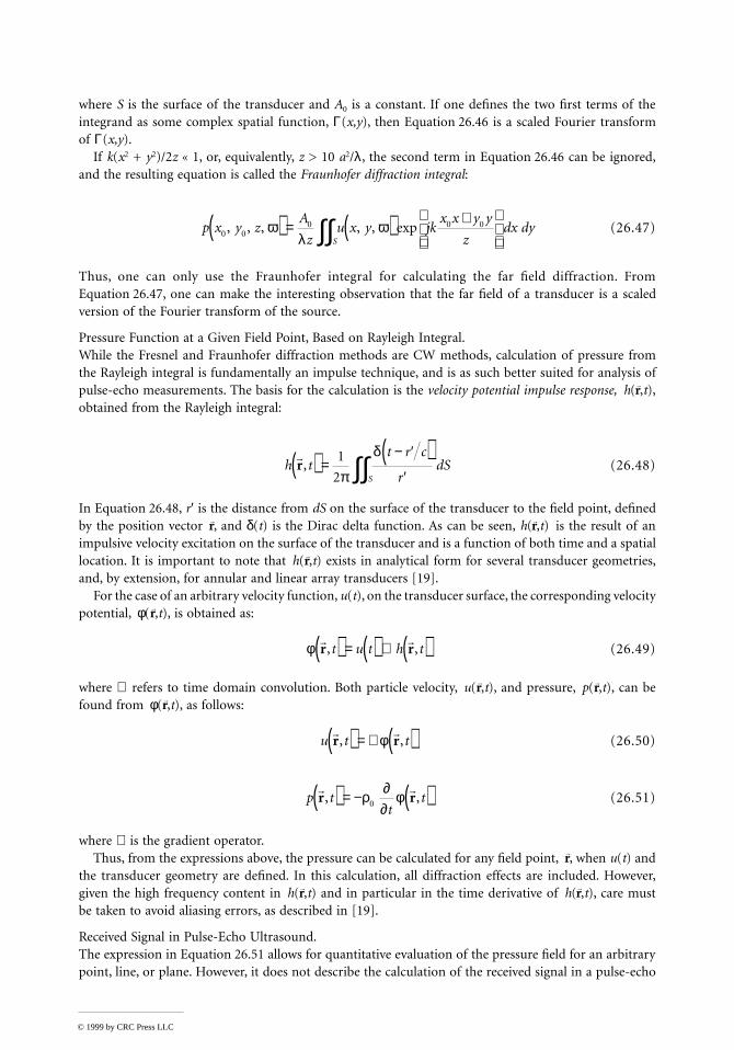
where S is the surface of the transducer and A0 is a constant. If one defines the two first terms of theintegrand as some complex spatial function, Γ(x,y), then Equation 26.46 is a scaled Fourier transformof Γ(x,y).

If k(x2 + y2)/2z « 1, or, equivalently, z > 10 a2/λ, the second term in Equation 26.46 can be ignored,and the resulting equation is called the Fraunhofer diffraction integral:

(26.47)

Thus, one can only use the Fraunhofer integral for calculating the far field diffraction. FromEquation 26.47, one can make the interesting observation that the far field of a transducer is a scaledversion of the Fourier transform of the source.

Pressure Function at a Given Field Point, Based on Rayleigh Integral.While the Fresnel and Fraunhofer diffraction methods are CW methods, calculation of pressure fromthe Rayleigh integral is fundamentally an impulse technique, and is as such better suited for analysis ofpulse-echo measurements. The basis for the calculation is the velocity potential impulse response, h(→r,t),obtained from the Rayleigh integral:

(26.48)

In Equation 26.48, r′ is the distance from dS on the surface of the transducer to the field point, definedby the position vector →r, and δ(t) is the Dirac delta function. As can be seen, h(→r,t) is the result of animpulsive velocity excitation on the surface of the transducer and is a function of both time and a spatiallocation. It is important to note that h(→r,t) exists in analytical form for several transducer geometries,and, by extension, for annular and linear array transducers [19].

For the case of an arbitrary velocity function, u(t), on the transducer surface, the corresponding velocitypotential, φ(→r,t), is obtained as:

(26.49)

where ⊗ refers to time domain convolution. Both particle velocity, u(→r,t), and pressure, p(→r,t), can befound from φ(→r,t), as follows:

(26.50)

(26.51)

where ∇ is the gradient operator.Thus, from the expressions above, the pressure can be calculated for any field point, →r, when u(t) and

the transducer geometry are defined. In this calculation, all diffraction effects are included. However,given the high frequency content in h(→r,t) and in particular in the time derivative of h(→r,t), care mustbe taken to avoid aliasing errors, as described in [19].

Received Signal in Pulse-Echo Ultrasound.The expression in Equation 26.51 allows for quantitative evaluation of the pressure field for an arbitrarypoint, line, or plane. However, it does not describe the calculation of the received signal in a pulse-echo

p x y zA

zu x y jk

x x y y

zdx dy

S0 0

0 0 0, , , , , expωλ

ω( ) = ( ) +

∫∫

h tt r c

rdS

S

rr,( ) =

π

− ′( )′∫∫1

2

δ

φr rr r, ,t u t h t( ) = ( ) ⊗ ( )

u t tr rr r, ,( ) = ∇ ( )φ

p tt

tr rr r, ,( ) = − ∂

∂ ( )ρ φ0


system. Consider a small planar reflector, placed in a homogeneous medium, and referred to as dR. Thereflector has the area dA. The dimensions of dR must be small with respect to the shortest wavelengthin the insonifying pulse. The location and the orientation of the planar reflector is given by →r and →n,respectively, where n is a unit normal vector to the small reflector.

The voltage from the receiving transducer in a pulse-echo system due to dR is termed d v(→r,t) and canbe determined when u(t) is specified. The electro-acoustic transfer function for both the transmittingand the receiving transducer is assumed to be unity for all frequencies. For the case when the acousticimpedance of dR is much higher than that of the medium, d v(→r,t) is given as [20]:

(26.52)

In Equation 26.52, A0 is determined by the reflection coefficient of the reflector. The term cos[ψ(→r)] is acorrection term (obliquity factor) where ψ(→r ) is the angle between n and the propagation direction of thewave field at →r. For an extended surface, the received voltage can be found by decomposing the surfaceinto small reflectors and calculating the total received signal as the sum of the contributions from all thesmall reflectors. An efficient numerical technique for this type of integration has been developed [21].

References

1. C. M. Fortunko and D. W. Fitting, Appropriate ultrasonic system components for NDE of thickpolymer-composites, Review of Progress in Quantitative Nondestructive Evaluation, Vol. 10B. NewYork: Plenum Press, 1991, 2105-2112.

2. C. R. Hill, Medical imaging and pulse-echo imaging and measurement, in C.R. Hill (ed.) PhysicalPrinciples of Medical Ultrasound, New York: Halsted Press, 1986, chaps. 7 and 8, 262-304.

3. L. C. Lynnworth, Ultrasonic Measurements for Process Control, San Diego: Academic Press, 1989,53-89.

4. L. E. Kinsler, A. R. Frey, A. B. Coppens, and J. V. Sanders, Fundamentals of Acoustics, 3rd. ed., NewYork: John Wiley, 1982, 106.

5. J. D. Achenbach, Wave Propagation in Elastic Solids, 1st ed., New York: Elsevier Science, 1975, 123.6. L. E. Kinsler, A. R. Frey, A. B. Coppens, and J. V. Sanders, Fundamentals of Acoustics, 3rd. ed., New

York: John Wiley, 1982, 115-117.7. L. E. Kinsler, A. R. Frey, A. B. Coppens, and J. V. Sanders, Fundamentals of Acoustics, 3rd. ed., New

York: John Wiley, 1982, 127-133.8. J. Saniie and N. M. Bilgutay, Quantitative grain size evaluation using ultrasonic backscattered

echoes, J. Acoust. Soc. Am., 80, 1816-1824, 1986.9. E. P. Papadakis, Scattering in polycrystalline media, in P. D. Edmonds (ed.) Ultrasonics, New York:

Academic Press, 1981, 237-298.10. S. M. Handley, M. S. Hughes, J. G. Miller, and E. I. Madaras, Characterization of porosity in

graphite/epoxy laminates with polar backscatter and frequency dependent attenuation, 1987 Ultra-sonics Symp., 1987, 827-830.

11. J. C. Bamber, Attenuation and absorption, in C.R. Hill (ed.), Physical Principles of Medical Ultra-sound, New York: Halsted Press, 1986, 118-199.

12. L. E. Kinsler, A. R. Frey, A. B. Coppens, and J. V. Sanders, Fundamentals of Acoustics, 3rd. ed., NewYork: John Wiley, 1982, 176-185.

13. M. O’Donnell, L. J. Busse, and J. G. Miller, Piezoelectric transducers, in P. D. Edmonds (ed.),Ultrasonics, New York: Academic Press, 1981, 29-65.

d v t Ac

h t h tt

u t dA

A u tc t

h t h t dA

rr

r r

r r r

rr

r r

r r r

,cos

, ,

cos , ,

( ) =( )[ ] ( ) ⊗ ( ) ⊗ ∂

∂( )

= ( )[ ] ( ) ⊗ ∂∂

( ) ⊗ ( )( )

0 0

0

2

2

00

0

2

2

ρψ

ψ ρ


14. IEEE Standard on Piezoelectricity, IEEE Trans. Sonics Ultrasonics, 31, 8–55, 1984.15. G.S. Kino, Acoustic Waves, Englewood Cliffs, NJ: Prentice-Hall, 1987, 17-83 and 554-557.16. L. C. Lynnworth, Ultrasonic Measurements for Process Control, San Diego, CA: Academic Press,

1989, 245-368.17. L. C. Lynnworth, Ultrasonic Measurements for Process Control, San Diego, CA: Academic Press,

1989, 537-557.18. V. M. Ristic, Principles of Acoustic Devices, New York: John Wiley & Sons, 1983, 316-320.19. D. P. Orofino and P. C. Pedersen, Multirate digital signal processing algorithm to calculate complex

acoustic pressure fields, J. Acoust. Soc. Am., 92, 563-582, 1992.20. A. Lhemery, Impulse-response method to predict echo responses from targets of complex geometry.

I. Theory, J. Acoust. Soc. Am., 90, 2799-2807, 1991.21. S. K. Jespersen, P. C. Pedersen, and J. E. Wilhjelm, The diffraction response interpolation method,

IEEE Trans. Ultrasonics, Ferroelectrics, and Frequency Control, 45, Nov. 1998.

Further Information

L. C. Lynnworth, Ultrasonic Measurements for Process Control, San Diego, CA: Academic Press, 1989, anexcellent overview of industrial applications of ultrasound.

L. E. Kinsler, A. R. Frey, A. B. Coppens, and J. V. Sanders, Fundamentals of Acoustics, 3rd. ed., New York:John Wiley & Sons, 1982, a very readable introduction to acoustics.

P. D. Edmonds (ed.), Ultrasonics, (Vol. 19 in the series: Methods of Experimental Physics). New York:Academic Press, 1981, in-depth description of ultrasound interaction with many types of materials,along with discussion of ultrasound measurement approaches.

J. A. Jensen, Estimation of Blood Velocities Using Ultrasound, Cambridge, UK: Cambridge University Press,1996, a very up-to-date book about ultrasound Doppler measurement of flow and the associatedsignal processing.

E. P. Papadakis (ed.), Ultrasonic Instruments and Devices: Reference for Modern Instrumentations, Tech-niques, and Technology, in the series Physical Acoustics, Vol. 40, New York: Academic Press, 1998.

F. W. Kremkau, Diagnostic Ultrasound: Principles and Instruments, 5th ed., Philadelphia, PA: W. B.Saunders Co., 1998, a very readable and up-to-date introduction to medical ultrasound.


Pressure and Sound Measurement - autex.spb.su

Documents

Transcript of Pressure and Sound Measurement - autex.spb.su