Preserving order observers for nonlinear systems · Interval observers, which consist of a couple...

INTERNATIONAL JOURNAL OF ROBUST AND NONLINEAR CONTROLInt. J. Robust. Nonlinear Control 2012; 00:1–31Published online in Wiley InterScience (www.interscience.wiley.com). DOI: 10.1002/rnc

Preserving order observers for nonlinear systems

Jesus D. Aviles∗,† and Jaime A. Moreno∗,‡

∗Coordinacion Electrica y Computacion. Instituto de Ingenierıa - Universidad Nacional Autonoma de Mexico. CiudadUniversitaria CP 04510 Mexico, D.F., Mexico

SUMMARY

Preserving Order Observers provide an estimation that is always above or below the true variable and, inthe absence of uncertainties/perturbations, the estimation converges asymptotically to the true value of thevariable. In this paper we propose a novel methodology to design preserving order observers for a classof nonlinear systems in the nominal case or when perturbations/uncertainties are present. This objectiveis achieved by combining two important systemic properties: dissipativity and cooperativity. Dissipativityis used to guarantee the convergence of the estimation error dynamics, while cooperativity of the errordynamics assures the order preserving properties of the observer. The use of dissipativity for observerdesign offers a big flexibility in the class of nonlinearities that can be considered while keeping the designsimple: it leads in many situations to the solution of a Linear Matrix Inequality (LMI). Cooperativity of theobserver leads to a LMI. When both properties are considered simultaneously the design of the observercan be reduced, in most cases, to the solution of both a Bilinear Matrix Inequality (BMI) and a LinearMatrix Inequality (LMI). Since a couple of preserving order observers, one above and one below, providean interval observer, the proposed methodology unifies several interval observers design methods. Thedesign methodology has been validated experimentally in a three-tanks system, and it has also been testednumerically and compared to an example from the literature. Copyright c© 2012 John Wiley & Sons, Ltd.

Received . . .

KEY WORDS: Interval Observers; Dissipative Observers; Cooperative Systems

1. INTRODUCTION

Observers provide a state variables estimation which converges asymptotically to their true values,at least when the plant model is perfectly known and/or no unknown disturbances are acting on thesystem. One drawback for certain applications is the fact that during the time span of convergenceit is not possible to trust in the estimation given by the observer. Decisions taken on the basis ofsuch estimation can lead to bad behavior in control (recall the use of saturating functions to avoidthe destabilizing effect in output feedback), or to wrong decisions in failure detection.

∗Correspondence to: Coordinacion Electrica y Computacion. Instituto de Ingenierıa - Universidad Nacional Autonomade Mexico. Ciudad Universitaria CP 04510 Mexico, D.F., Mexico.†Email: [email protected], [email protected]‡Email: [email protected]

Copyright c© 2012 John Wiley & Sons, Ltd.

Prepared using rncauth.cls [Version: 2010/03/27 v2.00]

2 J. D. AVILES AND J. A. MORENO

This situation is even worse when (non vanishing) uncertainties and/or perturbations are present.Since in this case it is not possible to construct a continuous observer without error, an alternativein many applications would be to have an estimation of a state variables that is always above orbelow the true value. This would allow, for example, to send an alarm signal when the temperatureof a nuclear reactor is about to reach the maximal critical value before it really reaches it, if theestimated temperature would be guaranteed above the true temperature. Such behavior can beobtained by a Preserving Order Observer, defined as an observer whose estimates always stay aboveor below the true state trajectory and, in the absence of uncertainites/perturbations, the estimationerror converges asymptotically to zero. Preserving order (or monotone) systems have very importantproperties, and they have been studied since several decades in mathematics and control [2, 14], ofwhich Cooperative systems build an important subclass. Although monotone systems have found agrowing interest in modeling and control, relatively few works on its use for observation purposeshave appeared.

Interval observers, which consist of a couple of preserving order observers, one giving an upperand the other a lower estimation of the state, have been proposed in the literature to provideguaranteed bounds at any instant of time for the states of an uncertain dynamical system. The firstapplication of the preserving order observers appeared in [12, 25], where interval observers areintroduced and applied to a class of nonlinear systems with uncertainties. They have been mainlyapplied to the estimation of parameters or non measurable variables in biological systems, for whichobservation issues are very challenging due to the limited availability of on-line sensors and theuncertainties related to the model dynamics. Experimental validation of Interval Observers has beenalso reported in [1] for highly uncertain bioreactors. A combination of interval observers and the socalled asymptotic observers [5, 9, 6] is proposed in [26], where the state observation for bioprocessesunder uncertain process parameters and/or process inputs is solved, without requiring the knowledgeof the process kinetics.

One interesting feature of interval observers is that they allow the comparison of the estimates ofseveral interval observers: the best upper bound is the lowest of the upper bounds, and vice versa forthe lower bounds. This has lead to the development of bundles of interval observers [6, 19], whichconsist of several interval observers running in parallel and the best estimate is taken at each timeinstant. In these bundles some estimates can be unstable. In this case the preserving order observersare called framers, since they do not have any stability properties. Recently in [20] a robust intervalobserver to estimate the unknown variables of uncertain chaotic systems is presented.

Since cooperativity is a coordinate dependent property, it is possible to use coordinatetransformations to obtain interval observers in appropriate coordinates. This idea has been usedrecently in [17, 18] to show that it is possible to design an exponentially convergent interval observerfor any Linear Time Invariant System, with additive perturbations, by using a linear time-varyingcoordinate transformation.

The objective of this paper is to pursue the line of research initiated in [12] (see also [19, 20]),for designing interval observers in the original coordinates of the system. The main idea is to mergethe dissipative observer design methodology, introduced by one of the authors several years ago[21, 22, 23, 27], with the basic idea of making the observer error system a cooperative one (see[4]), so that the observer preserves the order and converges to the true values, in the nominal case,i.e. in the absence of perturbations or uncertainties. For the perturbed case, the convergence will

Copyright c© 2012 John Wiley & Sons, Ltd. Int. J. Robust. Nonlinear Control (2012)Prepared using rncauth.cls DOI: 10.1002/rnc

PRESERVING ORDER OBSERVER 3

be weakened to the practical one: the observation error is Input-to-State Stable with respect to theperturbing signal. Moreover, the estimation error is required to be cooperative with respect to theperturbation. One of the advantages of using the dissipative observer design method resides in thefact that it is very flexible and unifies several observer design methods known to date, as for examplethe High-Gain Observer or the Circle-Criterion Observer design methods [21, 22, 23, 27].

Thus we consider a class of nonlinear systems, in absence and in presence of perturbations, forwhich dissipative observers can be designed, and a preserving order property will be imposed torender the estimation error of the observer cooperative. These systems are an extension of thoseproposed in [12], where interval observers were introduced. A first step consists in taking the errordynamics and to decompose it into a linear time invariant subsystem and a nonlinear time varyingfeedback. If the nonlinearity is dissipative with respect to a quadratic supply rate, the linear part mustbe designed to be dissipative with respect to a related supply rate, to assure exponential stability ofthe closed loop [21, 22, 23, 27]. Likewise, if the observation error dynamics is a cooperative system(with respect to the uncertainties/perturbations in case they exist) then the trajectories of the errorare assured to preserve the order and therefore the observer estimate dynamically upper or lowerbounds for the states, depending on the order of the initial error. Therefore, in a second step theestimation error will be made cooperative. Thus, preserving order observers for nonlinear systemsfulfill the two characteristics: observers preserve the order and the error estimation converges tozero in the absence of uncertainties/perturbations, or the error will be ultimately bounded for theperturbed case. These estimators were defined as cooperative observers in [4]. To build an intervalobserver two preserving order observers will be run in parallel: one provides an upper while theother a lower estimation of the states. The design of these observers can be reduced, in most cases,to a linear matrix inequality (LMI) and a bilinear matrix inequality (BMI), which are standard toolsin control theory. The performance of the preserving order observers has been tested in severalnumerical simulations.

2. PRELIMINARIES

In this work two system properties will be used for the design of preserving order observers:i) cooperativity is an order preserving property [28, 2, 14], and it will be fundamental for theinterval observers, and ii) dissipativity [8, 31, 32] (see also [15] and [21]) will be used to assurethe convergence properties of the estimation error. Some relevant results in these fields will berecalled here.

2.1. Cooperative Systems

The symbol represents a partial order in a space of vectors or matrices. For vectorsx, y ∈ Rn, x y ⇔ xi − yi ≥ 0,∀ i ∈ 1, . . . , n, i.e. each component of x is greater or equalto the corresponding component of y. For matrices M,N ∈ Rn×m, M N ⇔Mij −Nij ≥0, , ∀ i, j ∈ 1, . . . , n. In particular, non negative vectors or matrices satisfy, x 0⇔ xi ≥0, ∀ i ∈ 1, . . . , n or M 0⇔Mij ≥ 0, ∀ i, j ∈ 1, . . . , n, respectively.



Cooperative systems [2, 14], which are a special class of monotone systems, are those whose stateand output trajectories preserve the partial order at every time, when the input signals (if they arepresent) and the initial states are (partially) ordered.

Definition 1Consider a nonlinear system

ΣNL

x = F (t, x, u) , x(0) = x0

y = H (t, x, u) ,(1)

where x ∈ Rn is the state, u ∈ Rm is the input, and y ∈ Rp is the output of the system. F is asmooth vector field and H is a smooth nonlinear function, both depending on the variables (t, x, u).We will assume that the system is complete, i.e. the trajectories exist for all positive times t ≥ t0.ΣNL is cooperative if whenever the initial states and the inputs are ordered, i.e.

x10 x20, u1 (t) u2 (t) , ∀t ≥ 0

it follows that the state and the output trajectories are ordered too, i.e.

x(t, t0, x

10, u

1 (t)) x

(t, t0, x

20, u

2 (t)),

H x(t, t0, x

10, u

1 (t)) H x

(t, t0, x

20, u

2 (t)),∀t ≥ t0 .

Note that when no inputs and outputs are present, the previous definition reduces to the classicalone, in which ordered initial states implies ordered state trajectories [28]. Smooth cooperativesystems can be characterized in a simple way.

Proposition 2 ([2])The system ΣNL in (1) is cooperative if and only if all the following conditions are satisfied:

(C1)[∂Fi∂xj

]M 0⇔ ∂Fi

∂xj≥ 0, ∀i 6= j ; (C2)

[∂Fi∂uj

] 0 ; (C3)

[∂Hi

∂xj

] 0 .

The symbolM 0 represents that

[∂Fi∂xj

]is Metzler, that is, the off-diagonal elements are non

negative. In the classical situation without inputs/outputs cooperativity is equivalent to condition(C1). Linear cooperative systems are specially easy to characterize:

Proposition 3 ([2])Consider the linear continuous time system

ΣL :

x = Ax+Bu , x (0) = x0

y = Cx ,(2)

where (x, u, y) ∈ Rn ×Rm ×Rp are the state, the input and the output vectors, respectively. Thesystem ΣL in (2) is cooperative if and only if,

(C1) AM 0⇔ aij ≥ 0, ∀i 6= j ; (C2) B 0 ; (C3) C 0 .



We recall that Positivity is a related property to cooperativity. A system is positive if wheneverthe input and the initial conditions are non negative the state and output trajectories will be also nonnegative, i.e. x0 0 and u (t) 0 implies that x (t, t0, x0, u (t)) 0 and H x (t, t0, x0, u (t)) 0.For Linear Systems cooperativity and positivity are equivalent properties, but this is not the case fornonlinear systems.

2.2. Dissipative Systems

As dissipativity will play a fundamental role in the convergence of the observers, some results (see[31, 32, 8, 21, 22, 23, 27]) are recalled.

Consider a (smooth) nonlinear system ΣNL in (1), where x ∈ Rn, u ∈ Rm, and y ∈ Rp the state,the input and the output vectors, respectively. Assume that F (t, 0, 0) = 0 and H(t, 0, 0) = 0. Afunction w (y, u) : Rm ×Rp → R, such that w (0, 0) = 0 is called a supply rate for ΣNL if w (y, u)

is locally integrable for all input-output pairs of ΣNL. ΣNL is said to be State Strictly Dissipativewith respect to the supply rate w (y, u) ( or for short SSD w) if there exists a continuouslydifferentiable, positive-definite function V : Rn → R, with V (0) = 0, called a storage function, anda constant ε > 0, such that along any trajectory of the system the dissipative inequality

V (x(t)) ≤ −εV (x(t)) + w(y(t), u(t)) (3)

is satisfied.We will consider only quadratic supply rates (see [31, 32]):

w (y, u) =

[y

u

]T [Q S

ST R

][y

u

](4)

where Q ∈ Rp×p, S ∈ Rp×m, R ∈ Rm×m and Q, R are symmetric. In this case the system is saidto be (Q,S,R)-SSD. In the case of LTI systems in (2) with quadratic supply rates in (4) there is noloss of generality if the storage function is restricted to be a positive-definite quadratic form

V = xTPx, P = PT > 0. (5)

This can be characterized by means of a LMI:

Lemma 4The system ΣL in (2) is state strictly dissipative (SSD) with respect to the supply rate w (y, u) in(4), or for short (Q,S,R)-SSD, iff there exist a matrix P = PT > 0 and a constant ε > 0 such that

[PA+ATP + εP PB

BTP 0

]−

[CTQC CTS

STC R

]≤ 0 . (6)

A time-varing nonlinearity f : [0,∞)×Rm → Rp (see [15, 21])

y = f (t, u) (7)



piece-wise continuous in t and locally Lipschitz in u, such that f (t, 0) = 0, is said to be dissipativewith respect to the supply rate w (y, u) in (4), or for short (Q,S,R)-D, if for every t ≥ 0 and u ∈ Rm,

w (y, u) = w (f (t, u) , u) ≥ 0 . (8)

We note that the classical sector conditions [15] for square nonlinearities, i.e., m = p, can berepresented in this form:

1. If f ∈ [K1,K2], i.e., (y −K1u)T

(K2u− y) ≥ 0, then it is (Q,S,R)-D with: (Q,S,R) =(−I, 12 (K1 +K2) ,− 1

2

(KT

1 K2 +KT2 K1

)).

2. If f ∈ [K1,∞], i.e., (y −K1u)Tu ≥ 0, then it is (Q,S,R)-D with: (Q,S,R) =(

0, 12I,−12

(K1 +KT

1

)).

A multivariable nonlinearity f can be (Qi, Si, Ri)-D for several triples (Qi, Si, Ri), i.e.,ωi(f(t, u), u) = fTQif + 2fTSiu+ uTRiu ≥ 0, for i = 1, 2, ..., µ [21]. In this case, it is easy tosee that f is

∑µi=1 θi(Qi, Si, Ri)-D for every θi ≥ 0, i.e., f is dissipative with respect to the supply

rate ωθ(f, u) =∑µ

i=1 θiωi(f, u). Note that the inequality (8) provides a characterization of thenonlinearity f , since it means that the graph of f is contained in the subspace corresponding tothe non negative eigenvalues of the quadratic form (Q,S,R). If the quadratic form (Q,S,R) ispositive semidefinite, then inequality (8) does not provide any information about the nonlinearity fand it is therefore of no use in what follows.

The following lemma, which is a generalization of the circle criterion of absolute stability for nonsquare systems, shows that the negative feedback interconnection of a LTI dissipative system witha (complementary) dissipative static nonlinearity is internally exponentially stable:

Lemma 5 ([21, 22])Consider the feedback interconnection

ΞS :

x = Ax+Bu, x(0) = x0

y = Cx

u = −f (t, y) .

(9)

If there exist (Q, S, R) such that f (t, y) is (Q,S,R)-D, and the linear subsystem of ΞS is(−R,ST ,−Q

)-SSD, then the equilibrium point x = 0 of ΞS is globally exponentially stable, , i.e.

there exist constants k > 0 and % > 0 such that for all x0

‖x (t)‖ ≤ k ‖x0‖ exp(−%t) . (10)

Now we consider system ΞS with external additive perturbations, i.e.

ΞP :

x = Ax+Bu+ b(t), x(0) = x0

y = Cx

u = −f (t, y)

(11)

where b (t) is an input signal. Trajectories of the system will not converge to the origin x = 0, but ifthe input signal b(t) is bounded, the trajectories will converge to a ball centered at the origin, with



a radius depending on the bound of b, and they will remain there for all future times. This is thecontent of the Input-to-State-Stability property:

Definition 6 ([15])System ΞP is said to be Input-to-State Stable (ISS) with respect to b (t) if there exist a class KLfunction β, a class K function γ such that for any initial state x(t0) and any bounded input b(t), thesolution x(t) exists for all future times t ≥ t0 and satisfies

‖x (t)‖ ≤ β(‖x(t0)‖ , t− t0) + γ

(sup

t0≤τ≤t‖b(τ)‖

)

Lemma 7Consider the system ΞP and suppose that the conditions of Lemma 5 are satisfied. Under theseconditions system ΞP is ISS with respect to b.

ProofWe give the proofs of Lemmata 5 and 7. By hypothesis (4) is satisfied with

(−R,ST ,−Q

). Take

V (x) = xTPx as Lyapunov-like function candidate for the closed loop system. The time derivativeof V (x) along the solutions of ΞP is V = (Ax+Bu)

TPx+ xTP (Ax+Bu) + 2xTPb(t), or,

because of (6) and (11)

V =

[x

u

]T [PA+ATP PB

BTP 0

][x

u

]+ 2xTPb(t)

≤

[x

−f

]T [−CTRC CTST

SC −Q

][x

−f

]− εxTPx+ 2xTPb(t)

= −

[f

y

]T [Q S

ST R

][f

y

]− εV (x) + 2xTPb(t) ≤ −εV (x) + 2xTPb(t) ,

since f is (Q,S,R)-dissipative. When the perturbation vanishes, i.e. b(t) = 0, then V ≤ −εV and,using the comparison Lemma [15], it follows that

V (x (t)) ≤ V (x(0)) e−εt .

This means that

λmin (P ) ‖x(t)‖22 ≤ xT (t)Px(t) ≤ xT (0)Px(0)e−εt ≤ λmax (P ) ‖x(0)‖22e−εt ,

where λmin,max(P ) are the smallest and the greatest eigenvalues of P , respectively. Therefore

‖x(t)‖2 ≤

√λmax (P )

λmin (P )‖x(0)‖2e−

ε2 t ,

so that x = 0 is a globally exponential equilibrium point. This finishes the proof of Lemma 5.



When b is different from zero the inequality V ≤ −εV + 2xTPb can be rewritten, for anyθ ∈ (0, 1), as

V (x) ≤ −(1− θ)εV − θεxTPx+ 2xTPb

≤ −(1− θ)εV − θελmax(P )‖x‖22 + 2λmax(P )‖b‖2‖x‖2≤ −(1− θ)εV + λmax(P )‖x‖2(2‖b‖2 − θε‖x‖2)

≤ −(1− θ)εV, ∀‖x‖2 ≥2

θε‖b‖2 .

Applying [15, Theorem 4.19] it follows that ΞP is ISS with respect to b(t).

3. PRESERVING ORDER OBSERVERS

For a preserving order observer the estimated state x (t) is always above (or below) the true statevariable x (t) of the plant, i.e. either x (t) x (t) or x (t) x (t).

Definition 8 (Preserving Order Observer)Consider a nonlinear system

ΣNLP : x = F (t, x, u, w) , y = H (t, x, u) , x(0) = x0 ,

where x ∈ Rn, u ∈ Rm is a known input, y ∈ Rp and w ∈ Rq is an unknown input, representinguncertainties and/or perturbations acting on the system. F and H are smooth and we will assumethat the system is complete. The dynamical system

ΩNLP : ˙x = Φ (t, x, u, y, w) , x(0) = x0 ,

is an Upper (Lower) Preserving Order Observer, for system ΣNLP if (i) it is complete. (ii)The estimation error e (t) = x (t)− x (t) converges globally and asymptotically to zero when theperturbation is identically zero, i.e. w (t) = 0. (iii) Whenever the initial states of the observer aregreater (smaller) than the initial states of the plant, i.e. x0 x0 (x0 x0), the estimated statewill be greater (smaller) than the state of the plant for all future times and inputs (u,w), i.e.x (t, t0, x0, u, y (t)) x (t, t0, x0, u, w (t)) or ( x (t, t0, x0, u, y (t)) x (t, t0, x0, u, w (t))).

Although the completeness condition is not strictly necessary, it simplifies the presentation andit also seems reasonable for physical systems. An interval observer [17, 18] can be obtained withtwo preserving order observers: one upper and the other lower bounding the states of the plant. Ifwe dispense of the convergence condition (ii), then a framer will be obtained.

Condition (ii) in Definition 8 is a convergence condition on the observer, while condition (iii) is acooperativity condition on the estimation error. In order to guarantee the convergence of the observerwe will make use of the the dissipativity theory. This idea has been already proposed by one of theauthors [21, 22, 27] to design observers for a class of nonlinear systems. For the same class ofsystems we extend the method in order to make the observer not only convergent, but also orderpreserving [4]. We consider first the case of systems without perturbations and then a modification



will be introduced to the observer in order to assure the order preserving property despite of theperturbation.

3.1. Preserving Order Observers for nonlinear systems: The nominal case

Consider the nonlinear plant (without uncertainties/perturbations)

ΠS :

x = Ax+Gf (σ; t, y, u) + ϕ (t, y, u) ,

σ = Hx, x (0) = x0

y = Cx

(12)

where x ∈ Rn is the state, y ∈ Rq is the measured output, σ ∈ Rr is a (not necessarily measured)linear function of the state, u ∈ Rp is the input, f (σ; t, y, u) ∈ Rm is a nonlinear function locallyLipschitz in σ, depending on t and the measured variables u and y, and ϕ is a nonlinear functionlocally Lipschitz in (u, y) and piecewise continuous in t. We propose here a full order observer[21, 22, 27] for ΠS in (12) of the form

ΠO :

˙x = Ax+ L (y − y) +Gf (σ +N (y − y) ; t, y, u) + ϕ (t, y, u) ,

σ = Hx, x (0) = x0

y = Cx

(13)

where x ∈ Rn is the estimate of x in (12) and the matrices L ∈ Rn×q and N ∈ Rr×q have tobe designed. The state estimation error is defined by e , x− x, the output estimation error byy , y − y, and the functional estimation error by σ , σ − σ. The dynamics of the observation errorare given by

e = (A+ LC) e+G [f (σ +N (y − y) ; t, y, u)− f (σ; t, y, u)]

y = Ce

σ = He

(14)

with e (0) = e0 = x0 − x0. Note that σ +N (y − y) = Hx+He+NCe = σ + (H +NC) e.Defining z , (H +NC) e = σ +Ny, a function of the estimation error e, and the incrementalnonlinearity

φ (z, σ; t, y, u) , f (σ; t, y, u)− f (σ + z; t, y, u) (15)

the dynamics of the error in (14) can be written as

ΠE :

e = ALe+Gv, e(0) = e0

z = HNe

v = −φ (z, σ; t, y, u) ,

(16)

where AL , A+ LC and HN , H +NC.The observer ΠO in (13) is an (upper/lower) preserving order observer for ΠS if the estimation

error dynamics ΠE satisfies two properties:

1. The origin e = 0 is a globally asymptotically stable equilibrium point, and2. The error system ΠE in (16) is cooperative (in the classical sense).



The first condition means that x (t)→ x (t) as t→∞. The last condition implies that

if x0 x0 =⇒ x (t) x (t) , ∀t ≥ 0

if x0 x0 =⇒ x (t) x (t) , ∀t ≥ 0 ,

i.e. the observer preserves the order, and the estimation is always above or below the true planttrajectory, depending on the initial condition. Note that the observer is upper and lower preservingorder. In the next paragraphs conditions ensuring these two properties will be given.

3.1.1. Convergence of the observer. The following theorem gives sufficient conditions forasymptotic stability of the origin of the error dynamics making use of the dissipativity theory:

Theorem 9 ([21, 22, 27])Suppose that the nonlinearity φ in (15) is (Qi, Si, Ri)-D for some finite set of (non positivesemidefinite) quadratic forms

ωi(φ, z) = φTQiφ+ 2φTSiz + zTRiz ≥ 0, for all σ, for i = 1, 2, ..., µ (17)

Suppose that there exist matrices L, N and a vector θ = (θ1, ..., θµ), θi ≥ 0, such that ΠE in(16) is

(−Rθ, STθ ,−Qθ

)-SSD with (Qθ, Sθ, Rθ) =

∑µi=1 θi(Qi, Si, Ri), that is, there exist matrices

P = PT > 0, L and N , a vector θ = (θ1, ..., θµ) 0 and ε > 0 such that the matrix inequality (MI)

[PAL +ATLP + εP +HT

NRθHN PG−HTNS

Tθ

GTP − SθHN Qθ

]≤ 0 (18)

is satisfied. Under these conditions the observer ΠO in (13) is globally exponentially stable for ΠS .

The proof of the Theorem is based on Lemma 5 (see the proof of Lemma 7). The DissipativeDesign of observers presented in the preceding Theorem 9 is very flexible in the kind ofnonlinearities considered for the system. Moreover, the inclusion of multiple quadratic forms(Qi, Si, Ri) to characterize this nonlinearity greatly enhances the possibilities of the method. Inparticular, several methods for observer design, well known in the literature, are special cases of thisdesign. As examples we mention the High-Gain Observer design [10], the circle criterion design [3],the Lipschitz observer design [24], et cetera. For more details we refer the reader to the references[21, 22, 27].

3.1.2. Cooperativity of the observation error. The observer in (13) designed according to Theorem9 is convergent, but it does not have any order preserving properties. In order to assure cooperativity,the error system ΠE in (16) has to be a cooperative system. In accordance to the characterizationgiven in Proposition 2 this will be the case if the Jacobian matrix of the vector field of ΠE is Metzler,i.e.

∂

∂eALe−Gφ (z, σ; t, y, u) = AL +G

∂f (z + σ; t, y, u)

∂zHN

M 0, ∀z, σ, t, y, u .



We obtain this last expression noting that from (15) and the equality z = HNe it follows that

−∂φ (z, σ; t, y, u)

∂e=∂f (z + σ; t, y, u)

∂e=∂f (z + σ; t, y, u)

∂zHN .

Note that this condition is equivalent to the fact that the matrix

M (z; t, y, u) , AL +GJ (z; t, y, u)HN

M 0 , ∀z ∈ Rr, ∀t, y, u (19)

is Metzler everywhere. Here J(z; t, y, u) = ∂f(z;t,y,u)∂z is the Jacobian matrix of the nonlinearity

of the plant ΠS in (12). The following Theorem provides sufficient conditions for the design of apreserving order observer for ΠS in absence of uncertainties/perturbations:

Theorem 10Consider the plant ΠS in (12), and assume that the nonlinearity φ in (15) is (Qi, Si, Ri)-Dissipativefor a finite number of quadratic forms, that is (17) holds. Suppose furthermore that there existconstant matrices P = PT > 0, L, N , a constant scalar ε > 0, and a vector θ = (θ1, ..., θµ), θi ≥ 0,such that:

1. The Dissipativity condition, that is the matrix inequality in (18) is satisfied, and

2. M (z; t, y, u)M 0 in (19) is Metzler ∀z ∈ Rr, ∀t, y, u.

Under these conditions the system Π0 in (13) is a globally exponentially convergent upper/lowerpreserving order observer for the plant ΠS .

ProofThe Convergence condition 1 is derived from Theorem 9 (see also the Proof of Lemmata 5 and 7).The cooperativity condition 2 follows from Proposition 2.

Note that the same system Π0 is an upper or a lower preserving order observer, depending ifthe initial condition of the observer is above (x0 x0) or below (x0 x0) the initial conditions ofthe plant, respectively. Since the initial condition of the plant is unknown, to initialize correctly theupper (lower) preserving order observer it is necessary to know an upper x+0 (lower x−0 ) bound ofthe possible initial conditions of the plant, i.e.

x−0 x0 x+0 . (20)

Selecting the initial condition of the upper (lower) preserving order observer as x0 x+0 (x0 x−0 )ensures the correct behavior.

In order to obtain simultaneously a lower and an upper estimate of the state trajectory, it isnecessary to built two preserving order observers and initialize them adequately. This constitutesan interval observer.

Note that the design of a preserving order observer imposes an additional cooperativity conditionto the usual one of convergence for a standard observer. As a consequence it is expected that: (i)The class of systems for which a preserving order observer can be designed is a proper subset of theones for which a convergent observer exist. (ii) The assignable dynamic properties of a preservingorder observer can be more restricted than those for a simple convergent observer. For example, it is



possible that for a system is possible to design a convergent observer with assignable convergencedynamics, but that the convergence dynamics of a preserving order observer (if it exists) are stronglyrestricted. The study of these issues is an important topic for further research. Note that to designa preserving order observer it is not necessary that the plant ΠS be cooperative. Finally, the resultsof the paper can be easily extended to the class of systems described by ΠS in (12) with systemmatrices depending on time or measurable signals y and u as long as the dissipative inequality issatisfied with constant values for P and ε. The observer matrices L and N can also be time-varying.

3.2. Preserving Order Observers for systems with uncertainties/perturbations

Consider now the plant in (12) on which additive perturbations are acting

ΨS :

x = Ax (t) +Gf (σ; t, y, u) + ϕ (t, y, u) + π (t, x) ,

σ = Hx (t) , x (0) = x0

y = Cx (t) ,

(21)

where π (t, x) ∈ Rn represents unknown exogenous variables or/and system uncertainties. If theobserver Π0 in (13) is used for the plant, then the resulting estimation error dynamics

ΠpE :

e = ALe+Gv − π (t, x) , e(0) = e0

z = HNe

v = −φ (z, σ; t, y, u) ,

will not converge to zero, if the perturbation is not vanishing. Moreover, since in general π (t, x)

is not an ordered input signal, the error dynamics will not be cooperative, and the estimated stateswill not be ordered with respect to the true states of the plant. Due to the presence of unknowninputs in the plant, it is unlikely to obtain an observer that provides exact estimation of the states. Ingeneral, we will then require the estimation error not to be convergent, but to be bounded when theuncertainty is bounded, and to converge when the perturbation vanishes. In order to obtain an upper(lower) preserving order observer it will be assumed that upper (lower) bounds for the perturbationπ(t, x) are known, so that π (t, x) satisfies

π+ (t, y) π (t, x) π− (t, y) ,∀t ≥ 0, ∀x, y , (22)

where π+ (t, y) and π− (t, y) are known Lipschitz continuous functions.Consider an upper ΨO+ (lower ΨO−) estimator for ΨS of the form

ΨO+ :

˙x+

= Ax+ +Gf (σ+ +N+ (y+ − y)) + L+ (y+ − y) + π+ (t, y) + ϕ(t, y, u)

σ = Hx+, x+ (0) = x+0y = Cx+

(23)

ΨO− :

˙x−

= Ax− +G f (σ− +N− (y− − y)) + L− (y− − y) + π− (t, y) + ϕ(t, y, u)

σ = Hx−, x− (0) = x−0y = Cx−

(24)



where x+ (x−) is the upper (lower) estimate of x. Matrices L+ ∈ Rn×q, N+ ∈ Rr×q (L− ∈ Rn×q,N− ∈ Rr×q) have to be designed in order to assure the required convergence and cooperativeproperties. Note that in ΨO+ the upper bound and in ΨO− the lower bound of the perturbation (22)have been introduced. This will allow the error dynamics to be cooperative. Defining the estimationerrors as e+ , x+ − x and e− , x− x− (and the other variables defined in a similar manner), theobservation error dynamics are given by

ΨE+

e+ = A+Le

+ +Gv+ + b+

z+ = H+Ne

+, e+(0) = e+0 0

v+ = −φ+ (z+, σ)

(25)

ΨE−

e− = A−Le− +Gv− + b−

z− = H−Ne−, e−(0) = e−0 0

v− = −φ− (z−, σ)

(26)

where A+L , A+ L+C, H+

N , H +N+C, A−L , A+ L−C, H−N , H +N−C and the incremen-tal nonlinearities φ+ (z+, σ) y φ− (z−, σ) are defined in a similar form as (15). The uncertaintyerrors

b+ , π+ (t, y)− π (t, x) 0 (27)

b− , π (t, x)− π− (t, y) 0 (28)

act as inputs on the systems ΨE+ in (25) and ΨE− in (26).Note that the observer ΨO+ in (23) (ΨO− in (24)) is an upper (lower) preserving order observer

for ΨS if the estimation error dynamics ΨE+ (ΨE−) satisfies two properties:

1. It is ISS with respect to b+ (b−), and2. The error system ΨE+ (ΨE−) is cooperative with input b+ (b−) and output e+ (e−).

The first condition means that the estimation error e+(t) (e−(t)) will be ultimately bounded by abound depending on b+ (b−) and that it will converge to zero if b+(t)→ 0 (b−(t)→ 0) as t→∞.The latter condition implies that

x+0 x0 =⇒ x+ (t) x (t) ,(x0 x−0 =⇒ x (t) x− (t)

), ∀t ≥ 0 ,

i.e. the observer preserves the order, and the trajectories of Ψ0+ (Ψ0−) are always above (below) thetrue trajectories of the plant, despite of the perturbations.

Note that here, in contrast to the nominal case, the upper (lower) preserving order observer is onlyone sided ordered. This means that x+0 x0 ; x+ (t) x (t) (x−0 x0 ; x− (t) x (t)).

The following Theorem states sufficient conditions for the design of a preserving order observer.We state the result only for the upper preserving order observer ΨO+ , but it is also valid for thelower preserving order observer ΨO− .

Theorem 11Consider the perturbed plant ΨS in (21), and assume that the nonlinearity φ+ in (15) is (Qi, Si, Ri)-Dissipative for a finite number of quadratic forms, that is (17) holds. Suppose furthermore that



there exist constant matrices P+ = P+T > 0, L+, N+, a constant scalar ε+ > 0, and a vectorθ+ = (θ+1 , ..., θ

+µ ), θ+i ≥ 0, such that:

1. The Dissipativity condition, that is the matrix inequality in (18) is satisfied, and

2. M (z; t, y, u)M 0 in (19) is Metzler ∀z ∈ Rr, ∀t, y, u.

Under these conditions the system ΨO+ in (23) is a globally ISS upper preserving order observerfor the plant ΨS .

ProofThe Convergence condition 1 is derived from Lemma 7. The cooperativity condition 2 follows fromProposition 2, by noting that the input and the output mappings are for our case the identity, andtherefore its Jacobian matrix is non negative.

Since both φ+ and φ− depend only on the same nonlinearity f it follows that if φ+ is (Qi, Si, Ri)-D then so is φ−. This also implies that if the conditions of the Theorem 11 are satisfied for ΨO+ ,they will be also satisfied for ΨO− with the same parameter values, and in particular, with the sameobserver matrices L+ = L− and N+ = N−. That means that if it is possible to design an upperpreserving order observer it will be also possible to design a lower preserving order observer, andvice versa. Moreover, both observers can have (but they do not have to) the same matrices L+ = L−

and N+ = N−.If both upper Ψ0+ in (23) and lower Ψ0− in (24) preserving order observers are run in parallel, if

there exist known bounds on the initial conditions (20) and on the perturbations (22) of the plant,and the observers are adequately initialized, then an interval observer is obtained for the perturbedplant ΨS , so that the next conditions hold:

x+0 x+0 x0 x

−0 x

−0 =⇒ x+ (t) x (t) x− (t) . (29)

Note that Theorem 11 can be seen as a generalization of Theorem 10. In fact, setting π+(t, y) ≡ 0

in the upper Ψ0+ in (23) and π−(t, y) ≡ 0 in the lower Ψ0− in (24) preserving order observers weobtain an interval observer in the nominal case. Moreover, the set of values for the observer matricesL andN that satisfy the conditions of Theorems 11 and 10 are the same, since the conditions in theseTheorems do not depend on the perturbation.

4. COMPUTATIONAL ISSUES

The design of preserving order (or interval) observers for the considered class of nonlinear systems,in the nominal case or in presence of uncertainties/perturbations, is reduced to the solution of twomatrix inequalities (see Theorems 10 and 11):

(i) Convergence requires to find matrices L, N , P = PT > 0, a constant ε > 0 and a vectorθ = (θ1, ..., θµ) 0 such that the Matrix Inequality (MI) (18) is satisfied.

(ii) Cooperativity requires that matrices L and N are such that the family of matrices M (·)M 0

in (19) is Metzler.

We will discuss some issues on the solution of these inequalities.



4.1. The Dissipativity Inequality (18)

The nature of the MI in (18) has been studied in [21, 22, 27]. Here we recall some results and providesome new ones. In general, inequality (18) is nonlinear in the unknowns (L,N, P, ε, θ). However,under some important conditions, (18) becomes a Linear Matrix Inequality (LMI) feasibilityproblem, for which a solution can be effectively found by several algorithms in the literature [11, 7]and in Matlab.

1. A first observation is that the product εP makes (18) nonlinear in the two unknowns ε and P .However, the bilinear term εP can be always replaced by the term εI , where I is the identitymatrix, that is linear in ε, without altering the feasibility of the MI in (18). To see this, assumethat there exist ε and P that satisfy (18). The MI (18) can be rewritten as

[PAL +ATLP + εI +HT

NRθHN PG−HTNS

Tθ

GTP − SθHN Qθ

]≤

[εI − εP 0

0 0

]. (30)

If ε ≤ λmin (P ) ε, then it follows that the left hand matrix in (30) is negative semidefinite.Conversely, a similar argument shows that if the left hand matrix in (30) is negativesemidefinite, then there exist an ε > 0 such that MI (18) is fulfilled. So both inequalities arein fact equivalent. For the further discussion we will assume that in (18) the term εP has beenreplaced by the term εI .

2. Further nonlinear terms in (18) are due to the terms SθHN and HTNRθHN , where bilinear

terms in θ and N appear, but also a quadratic term in N . If N is fixed, as for example forthe High-Gain Observer design, where N = 0 [21, 22], then (18) is an LMI in P, ε, PL, θ.Note that, once the values of P and PL have been obtained, then the value of L can be easilycalculated from L = P−1(PL), since P is invertible.

3. A further alternative is to fix θ. This is a natural situation when the nonlinearity φ is (Q,S,R)-Dissipative only for one quadratic form, that is (17) holds with µ = 1. This is always the caseif the nonlinearity f in (12) is scalar, i.e. m = r = 1, or if it is square (i.e. m = r) and thenonlinearities are decoupled, i.e. f(σ) = [f1(σ1), . . . , fm(σm)]. In these situations multiple(non trivial) dissipativity conditions for φ are impossible [22, 27]. We consider differentsituations:

(a) If Rθ = 0, for example if all Ri = 0, again (18) is an LMI in P, ε, PL,N . In somesituations it is possible to transform a problem with Rθ 6= 0 into one with Rθ = 0 bya loop transformation (see [27]).

(b) If Rθ > 0, and using Schur’s complement, one can transform inequality (18) into theequivalent Matrix Inequality

−R−1θ −HN 0

−HTN PAL +ATLP + εI PG−HT

NSTθ

0 GTP − SθHN Qθ

≤ 0 , (31)

that is again an LMI in P, ε, PL,N .



(c) If Rθ ≤ 0 a sufficient condition for (18) is the Matrix Inequality

[PAL +ATLP + εI PG−HT

NSTθ

GTP − SθHN Qθ

]≤ 0 ,

that is an LMI in P, ε, PL,N .

In general, a solution to (18) can be found by using specialized software for nonlinear MatrixInequality Problems, e.g. the software PENNON [16]. Alternatively, one can use an efficient LMIsolver, fixing iteratively the matrix N , or the vector θ in cases (3a-3c) above.

4.2. The Cooperativity Inequality (19)

Consider the set J ⊂ Rm×r of all values taken by the Jacobian of the nonlinearity f , i.e.

J =

Γ ∈ Rm×r

∣∣Γ = J (z; t, y, u) =∂f (z; t, y, u)

∂z,∀z, t, y, u

. (32)

Inequality (19) is an LMI in L,N , for every J ∈ J . However, since J is a set with an uncountableinfinite number of points, (19) corresponds to an infinite number of LMIs. This is a difficult task,and it is of interest to reduce the number of LMIs to be checked to a finite number. In the followingparagraphs it will be shown that it is possible to find a finite number q of points Ωi in Rm×r such

that if inequality (19) is satisfied at all these points, i.e. AL +GΩiHN

M 0 ∀i = 1, . . . , q, then it

will be satisfied for all J ∈ J .The basic idea is very simple. We assume that the set J is bounded. This is the case if the

nonlinearity f (σ; t, y, u) is globally Lipschitz in σ, uniformly in (t, y, u). In this case, it is alwayspossible to find a polytope that contains J (take for example a hypercube containing J ). Due to theconvexity of inequality (19) it suffices to check it on the vertices of such polytope to conclude that itis satisfied on the whole set J . Refinement of the polytope, by adding extra vertices while reducingits size, will provide less conservative conditions.

We will show that if the nonlinearity φ (z;σt, y, u) = f (σ; t, y, u)− f (z + σ; t, y, u), definedin (15), satisfies a sector condition, i.e. if there exist two constant matrices K1 ∈ Rm×r andK2 ∈ Rm×r such that for all σ, t, y, u and all z the inequality

[φ (z;σ, t, y, u)−K1z]T

[K2z − φ (z;σ, t, y, u)] ≥ 0 (33)

is satisfied, then the set of values at which the inequality (19) has to be verified can be considerablyreduced. In fact, we will show that under condition (33) the set J is contained in a convex set Υ,and that it is only necessary to verify the inequality (19) on the boundary of Υ. This is establishedin the following proposition.

Proposition 12Let z → f(z; t, y, u) : Rr → Rm be a multivariable function, continuous in t, y, u and continuouslydifferentiable in z. Suppose that φ (z;σ, t, y, u) = f (σ; t, y, u)− f (z + σ; t, y, u) is in the sector[K1 , K2], i.e. for some constant matrices K1 ∈ Rm×r and K2 ∈ Rm×r (33) is fulfilled. If thematrices

AL +G∆HN

M 0 (34)



are Metzler for all ∆ ∈ Υf , defined by

Υf =

Γ ∈ Rm×r∣∣ (Γ +K1)

T(K2 + Γ) = 0

, (35)

then condition M(z; t, y, u)M 0 in (19) is satisfied ∀ z ∈ Rr, and all t, y, u.

ProofThe demonstration is given in three parts:

(i) We first show that when the nonlinearity φ belongs to the sector [K1, K2], then J ⊂ Υ, wherethe convex set

Υ ,

Γ ∈ Rm×r∣∣ [Γ +K1]

T[K2 + Γ] ≤ 0

. (36)

By the mean value theorem (see e.g. [30, p. 51]) one can write

φ(z;σ, t, y, u) = −(∫ 1

0

J (σ + θz; t, y, u) dθ

)z , (37)

where the matrixΘ (z;σ, t, y, u) ,∫ 1

0

J (σ + θz; t, y, u) dθ is continuous in all its arguments.

The sector condition (33) can therefore be equivalently expressed as

−(∫ 1

0

zT [J (σ + θz; t, y, u) +K1]T

[K2 + J (σ + θz; t, y, u)] zdθ

)≥ 0 . (38)

This implies that J ⊂ Υ. It is obvious that if (34) is satisfied for all ∆ ∈ Υ inequality (19)follows.

(ii) Now we show that Υ is a convex set. Convexity of Υ follows from the fact that the defininginequality of Υ, i.e. [Γ +K1]

T[K2 + Γ] ≤ 0, using Shur’s Lemma, can be rewritten as

[KT

1 K2 +K1Γ + ΓTK2 −ΓT

−Γ −I

]≤ 0 ,

that is an LMI in Γ.(iii) Finally we show that if (34) is satisfied for all ∆ ∈ Υf , the boundary of Υ, then it is also

satisfied for all ∆ ∈ Υ. For this note that if AL +G∆1HN

M 0 and AL +G∆2HN

M 0 for

two matrices ∆1 , ∆2 ∈ Υ, then it follows that for every scalar α ∈ [0 , 1]

α (AL +G∆1HN ) + (1− α) (AL +G∆2HN ) = AL +G (α∆1 + (1− α) ∆2)HN

M 0 ,

showing that the inequality (34) is convex in ∆. This implies that it suffices to check (34) onthe boundary of Υ.

Remark 13Recall that φ being in the sector [K1 , K2] is equivalent to φ being (Q, S, R)-Dissipative, where(Q,S,R) =

(−I, 12 (K1 +K2) ,− 1

2

(KT

1 K2 +KT2 K1

)).



A more general version of the Proposition, with basically the same proof, can be obtained in thefollowing form. When φ is (Q, S, R)-Dissipative, with Q < 0, then

φTQφ+ 2φTSz + zTRz =

∫ 1

0

zTJT (ϑ)QJ (ϑ)− 2JT (ϑ)S +R

zdϑ ≥ 0

where J (ϑ) = J (σ + ϑz; t, y, u). It is clear that J ⊂ Υ, where Υ is the set of matrices Γ ∈ Rm×r

such that

ΓTQΓ− 2ΓTS +R =

[R− ΓTS − STΓ ΓT

Γ −Q−1

]≥ 0 . (39)

Since Υ is convex, it is sufficient to check the inequality (34) on its boundary Υf , defined as the setof Γ ∈ Rm×r such that ΓTQΓ− 2ΓTS +R = 0.

Note also that if φ satisfies several dissipative conditions (Qi, Si, Ri), for i = 1, . . . , µ, withQi < 0, then the previous Proposition is valid for each sector condition with a boundary set Υfi. Tosimplify the presentation we will restrict ourselves in what follows to the case of one dissipativitycondition, or when the vector θ is fixed.

Proposition 12 reduces substantially the size of the set of matrices at which the cooperativitycondition (19) has to be checked. In particular, in the scalar case, i.e. r = m = 1, and σ →f(σ; t, y, u) : R→ R, the set Υ is the interval [K1, K2] and its boundary are the two extremepoints Υf = K1, K2. In this case it suffices to check (19) for just these two values of J . Asimilar situation occurs in the diagonal case, i.e. r = m and σ → f(σ; t, y, u) : Rm → Rm withσi → fi(σi; t, y, u) : R→ R for i = 1, . . . ,m, where Υf consists of a finite number of points.

Beyond these two simple cases, the number of points in Υf is not finite. In what follows wewill restrict our discussion to the case where Γ is a vector, i.e. r = 1, m > 1, since in this case thegeometrical interpretation is simple. However, the general idea can be extended to the matrix case.The set of vectors Γ ∈ Rm, satisfying expression in (39), i.e.

Υ ,

Γ ∈ Rm|ΓTQΓ− 2ΓTS +R ≥ 0

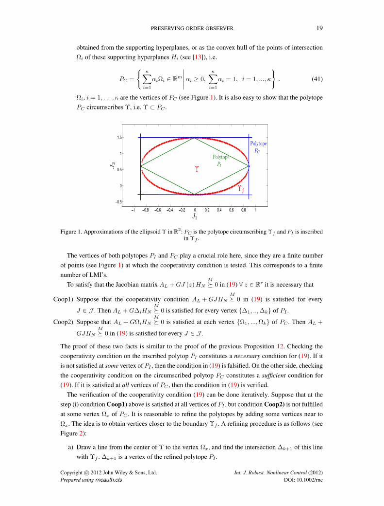
where Q < 0, represents an ellipsoid in Rm [7] (see Figure 1).Given an ellipsoid Υ we construct two convex polytopes:

(i) Select k > 1 points ∆i ∈ Υf ⊂ Rm on the boundary Υf of Υ, and construct the closed convexpolytopte PI ⊂ Rm as the convex hull (convex combination) of these points [13], i.e.

PI =

k∑

i=1

αi∆i ∈ Rm∣∣∣∣∣αi ≥ 0,

k∑

i=1

αi = 1, i = 1, ..., k

. (40)

∆i, i = 1, . . . , k are the vertices of PI . In particular, we select all the vertices of the ellipsoidas vertices of the polygon PI . In a refinement of PI further points on Υf are added to theset of vertices of PI . It is easy to see that the polytope PI is inscribed in Υ, i.e. PI ⊂ Υ (seeFigure 1).

(ii) At each vertex ∆i of PI there is a supporting hyperplane Hi, that is tangent to Υf . Thepolytope PC ⊂ Rm can be equivalently defined as the intersection of the closed half-spaces



obtained from the supporting hyperplanes, or as the convex hull of the points of intersectionΩi of these supporting hyperplanes Hi (see [13]), i.e.

PC =

κ∑

i=1

αiΩi ∈ Rm∣∣∣∣∣αi ≥ 0,

κ∑

i=1

αi = 1, i = 1, ..., κ

. (41)

Ωi, i = 1, . . . , κ are the vertices of PC (see Figure 1). It is also easy to show that the polytopePC circumscribes Υ, i.e. Υ ⊂ PC .

−1 −0.8 −0.6 −0.4 −0.2 0 0.2 0.4 0.6 0.8 1

−0.5

0

0.5

1

1.5

J1

J2

Υ

Υf

PolytopePC

PolytopePI

Figure 1. Approximations of the ellipsoid Υ in R2: PC is the polytope circumscribing Υf and PI is inscribedin Υf .

The vertices of both polytopes PI and PC play a crucial role here, since they are a finite numberof points (see Figure 1) at which the cooperativity condition is tested. This corresponds to a finitenumber of LMI’s.

To satisfy that the Jacobian matrix AL +GJ (z)HN

M 0 in (19) ∀ z ∈ Rr it is necessary that

Coop1) Suppose that the cooperativity condition AL +GJHN

M 0 in (19) is satisfied for every

J ∈ J . Then AL +G∆iHN

M 0 is satisfied for every vertex ∆1, ..,∆k of PI .

Coop2) Suppose that AL +GΩiHN

M 0 is satisfied at each vertex Ω1, ...,Ωk of PC . Then AL +

GJHN

M 0 in (19) is satisfied for every J ∈ J .

The proof of these two facts is similar to the proof of the previous Proposition 12. Checking thecooperativity condition on the inscribed polytop PI constitutes a necessary condition for (19). If itis not satisfied at some vertex of PI , then the condition in (19) is falsified. On the other side, checkingthe cooperativity condition on the circumscribed polytop PC constitutes a sufficient condition for(19). If it is satisfied at all vertices of PC , then the condition in (19) is verified.

The verification of the cooperativity condition (19) can be done iteratively. Suppose that at thestep (i) condition Coop1) above is satisfied at all vertices of PI , but condition Coop2) is not fulfilledat some vertex Ωx of PC . It is reasonable to refine the polytopes by adding some vertices near toΩx. The idea is to obtain vertices closer to the boundary Υf . A refining procedure is as follows (seeFigure 2):

a) Draw a line from the center of Υ to the vertex Ωx, and find the intersection ∆k+1 of this linewith Υf . ∆k+1 is a vertex of the refined polytope PI .



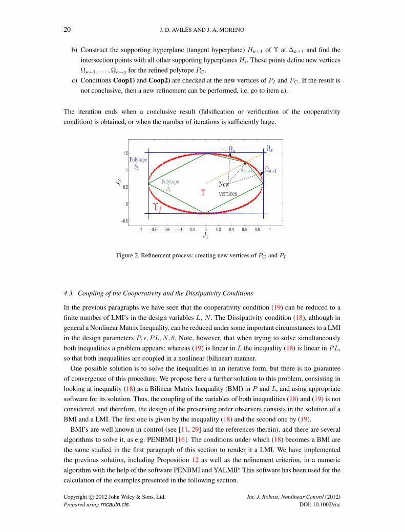
b) Construct the supporting hyperplane (tangent hyperplane) Hk+1 of Υ at ∆k+1 and find theintersection points with all other supporting hyperplanes Hi. These points define new verticesΩκ+1, . . . ,Ωκ+g for the refined polytope PC .

c) Conditions Coop1) and Coop2) are checked at the new vertices of PI and PC . If the result isnot conclusive, then a new refinement can be performed, i.e. go to item a).

The iteration ends when a conclusive result (falsification or verification of the cooperativitycondition) is obtained, or when the number of iterations is sufficiently large.

−1 −0.8 −0.6 −0.4 −0.2 0 0.2 0.4 0.6 0.8 1

−0.5

0

0.5

1

1.5

J1

J2

Ωx

Υ

Υf

Ωn

Ωn+1df,m+1

Newvertices

PolytopePC

PolytopePI

Figure 2. Refinement process: creating new vertices of PC and PI .

4.3. Coupling of the Cooperativity and the Dissipativity Conditions

In the previous paragraphs we have seen that the cooperativity condition (19) can be reduced to afinite number of LMI’s in the design variables L, N . The Dissipativity condition (18), although ingeneral a Nonlinear Matrix Inequality, can be reduced under some important circumstances to a LMIin the design parameters P, ε, PL,N, θ. Note, however, that when trying to solve simultaneouslyboth inequalities a problem appears: whereas (19) is linear in L the inequality (18) is linear in PL,so that both inequalities are coupled in a nonlinear (bilinear) manner.

One possible solution is to solve the inequalities in an iterative form, but there is no guaranteeof convergence of this procedure. We propose here a further solution to this problem, consisting inlooking at inequality (18) as a Bilinear Matrix Inequality (BMI) in P and L, and using appropriatesoftware for its solution. Thus, the coupling of the variables of both inequalities (18) and (19) is notconsidered, and therefore, the design of the preserving order observers consists in the solution of aBMI and a LMI. The first one is given by the inequality (18) and the second one by (19).

BMI’s are well known in control (see [11, 29] and the references therein), and there are severalalgorithms to solve it, as e.g. PENBMI [16]. The conditions under which (18) becomes a BMI arethe same studied in the first paragraph of this section to render it a LMI. We have implementedthe previous solution, including Proposition 12 as well as the refinement criterion, in a numericalgorithm with the help of the software PENBMI and YALMIP. This software has been used for thecalculation of the examples presented in the following section.



5. DESIGN EXAMPLES

To illustrate the design methodology and the performance of the preserving order observers, wewill present two examples. The first example shows an experimental validation in the classicalthree-tanks system. The second example compares in simulation our design with one example takenfrom the literature.

5.1. Experimental validation: The Three-Tanks system

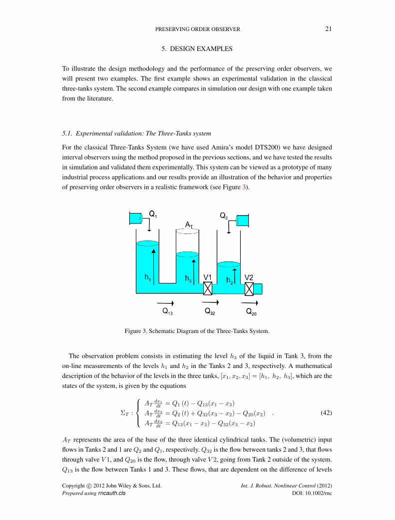
For the classical Three-Tanks System (we have used Amira’s model DTS200) we have designedinterval observers using the method proposed in the previous sections, and we have tested the resultsin simulation and validated them experimentally. This system can be viewed as a prototype of manyindustrial process applications and our results provide an illustration of the behavior and propertiesof preserving order observers in a realistic framework (see Figure 3).

Figure 3. Schematic Diagram of the Three-Tanks System.

The observation problem consists in estimating the level h3 of the liquid in Tank 3, from theon-line measurements of the levels h1 and h2 in the Tanks 2 and 3, respectively. A mathematicaldescription of the behavior of the levels in the three tanks, [x1, x2, x3] = [h1, h2, h3], which are thestates of the system, is given by the equations

ΣT :

ATdx1

dt = Q1 (t)−Q13(x1 − x3)

ATdx2

dt = Q2 (t) +Q32(x3 − x2)−Q20(x2)

ATdx3

dt = Q13(x1 − x3)−Q32(x3 − x2)

. (42)

AT represents the area of the base of the three identical cylindrical tanks. The (volumetric) inputflows in Tanks 2 and 1 areQ2 andQ1, respectively.Q32 is the flow between tanks 2 and 3, that flowsthrough valve V 1, and Q20 is the flow, through valve V 2, going from Tank 2 outside of the system.Q13 is the flow between Tanks 1 and 3. These flows, that are dependent on the difference of levels



of the tanks they connect, are described by:

Q32(x3 − x2) , K32 sgn (x3 − x2)√

2g |x3 − x2|

Q13(x1 − x3) , K13 (x1 − x3)

Q20(x2) , K20

√2gx2

where K13 = a13Sn, K32 = a32Sn and K20 = a20Sn. The values of these parameters for theexperimental setup used are listed in Table I. It is possible to write the (nominal) system in the

Parameters Numeric valuesSn 5×10−5 m2

g 9.81 m/s2

a13 8.5720a20 0.7026a32 0.48831AT

64.977 1/m2

Table I. Parameters for the Experimental setup of the Three-Tanks system ΣT .

form ΠS in (12) with matrices given by:

A =K31

AT

−1 0 1

0 0 0

1 0 −1

, G =

1

AT

0

−1

1

, H =

0

1

−1

T

, C =

[1 0 0

0 1 0

].

The known input vector u consists of the two input flows Q1 and Q2, i.e. u = [Q1 , Q2]T , and the

input/output injection vector ϕ (t, y, u), consisting of known signals affecting the dynamics of theplant, is given by

ϕ (t, y, u) =1

AT

Q1 (t)

Q2 (t)−Q20 (x2)

0

.

Finally, the (internal) nonlinearity in the model f (σ) is given by f (σ) , K32 sgn (σ)√

2g |σ|, andit depends on the variable σ = x2 − x3, which is linear function of the states, i.e. σ = Hx, and it isnot measurable, since it depends on the unmeasured state variable x3.

We will consider two scenarios for the interval observer design:

1. We consider that there are no uncertainties in the model description, and we design theobserver using the results of Subsection 3.1.

2. We consider a perturbation for the system consisting of a leak in Tank 3, flowing out of thesystem. It is possible to write the (perturbed) system in the form ΨS in (21) with the samematrices as for the nominal model and with a perturbation vector π(t, x) = [0, 0, π3(t)]T . Weknow that π3(t) lies between some values π− ≤ π(t) ≤ π+. We design an interval observerusing the results of Subsection 3.2.



5.1.1. Interval observer design for the Three-Tanks system. For both scenarios we design the sameobserver matrices L and N . The incremental nonlinearity φ defined in (15) is given by

φ (z, σ) = K32

(sgn (σ)

√2g |σ| − sgn (σ + z)

√2g |σ + z|

),

which is a scalar nonlinearity in the sector [−∞, 0]. Although it is possible to satisfy the conditionsof Theorem 10 using this sector, the required observer gains are very high. Since the infinityvalue is due to the lack of differentiability of the square root function in Q20, it is reasonableto consider a smooth approximation of this function, that has a finite slope in zero, withoutaltering the accuracy of the model to predict the experimental results. We have found that using anapproximating function, belonging to the the sector φ ∈ [−0.1 , 0], or equivalently, being (Q,S,R)-Dissipative with (Q,S,R) = (−1, −0.05, 0) reasonable experimental results are obtained, withgains implementable in practice. Using this data we solve both, the dissipative in (18) and thecooperative in (19) inequalities using a BMI solver†, and we have obtained as solutions the followingmatrices

L =

−518.317 53.9564

118.9967 −303.4840

122.9429 278.2979

, N =

[0 10

],

P =

18.6334 39.3332 39.3332

39.3332 84.2404 84.2334

39.3332 84.2334 84.2327

, ε = 0.1796 .

Since Theorem 10 is satisfied it is possible to design a preserving order observer, and thereforean interval observer by running in parallel two adequately initialized preserving order observers,one to upper estimate and the other to lower estimate the state trajectory. We have used the samegains for both observers, and thus L = L+ = L−, N = N+ = N−, P = P+ = P−, ε = ε+ = ε−.For comparison purposes an open-loop observer has been designed, i.e.,

L = 0 and N = 0.

Note that this open loop observer is also a preserving order observer, since the conditions ofTheorem 10 are satisfied with these values of L and N .

5.1.2. Experimental validation of the Interval observers. We have run three experiments on thesystem to test the two interval observers designed. The first two consider the nominal case, while inthe third experiment a leak in Tank 3 causes a perturbation for the observation problem.

Experiment 1: For this test we consider the case without a leak in Tank 3. The input flowshave been set constant with values Q0

1 = 2.4425× 10−5 m3

s and Q02 = 1.9889× 10−5 m3

s . The initialstates for the plant were x10 = 0.14 m, x20 = 0.04 m and x30 = 0.09 m, and the initial conditions

†we have used here PENBMI ’s software.



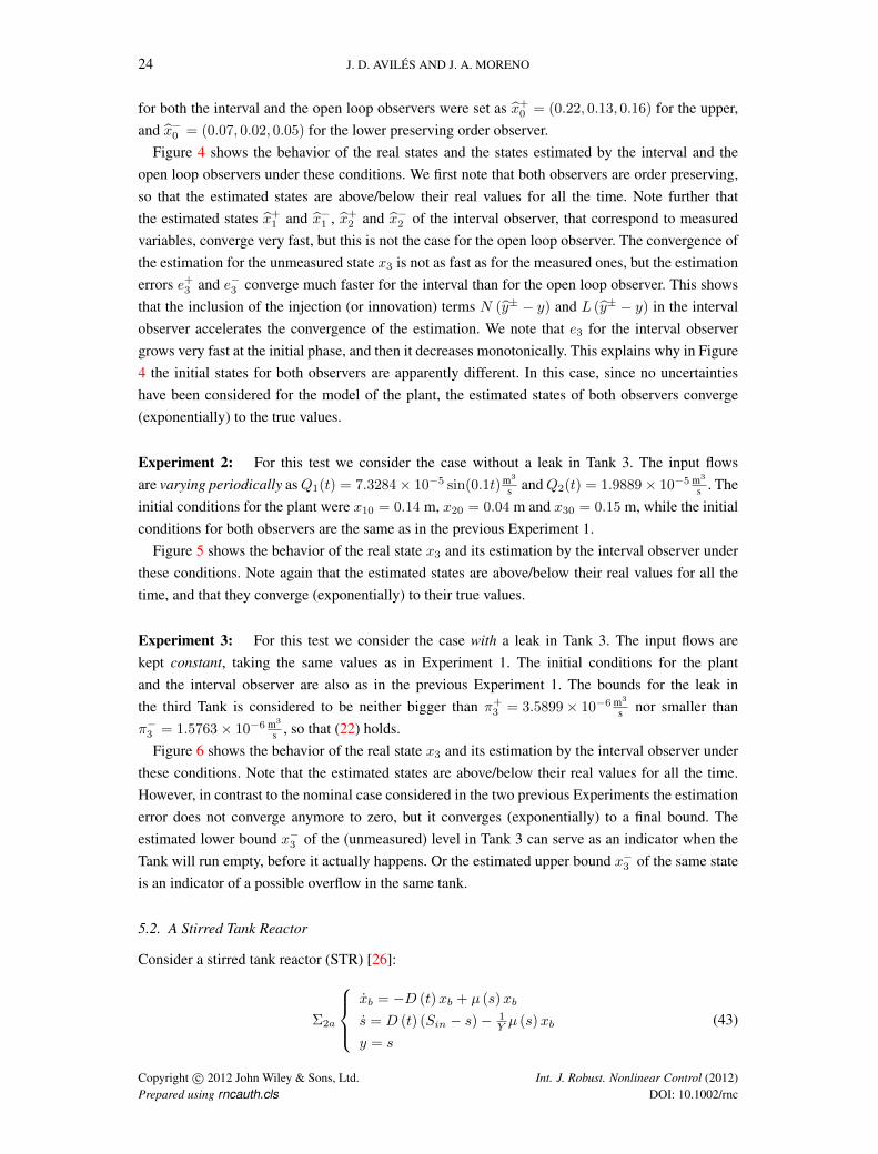
for both the interval and the open loop observers were set as x+0 = (0.22, 0.13, 0.16) for the upper,and x−0 = (0.07, 0.02, 0.05) for the lower preserving order observer.

Figure 4 shows the behavior of the real states and the states estimated by the interval and theopen loop observers under these conditions. We first note that both observers are order preserving,so that the estimated states are above/below their real values for all the time. Note further thatthe estimated states x+1 and x−1 , x+2 and x−2 of the interval observer, that correspond to measuredvariables, converge very fast, but this is not the case for the open loop observer. The convergence ofthe estimation for the unmeasured state x3 is not as fast as for the measured ones, but the estimationerrors e+3 and e−3 converge much faster for the interval than for the open loop observer. This showsthat the inclusion of the injection (or innovation) terms N (y± − y) and L (y± − y) in the intervalobserver accelerates the convergence of the estimation. We note that e3 for the interval observergrows very fast at the initial phase, and then it decreases monotonically. This explains why in Figure4 the initial states for both observers are apparently different. In this case, since no uncertaintieshave been considered for the model of the plant, the estimated states of both observers converge(exponentially) to the true values.

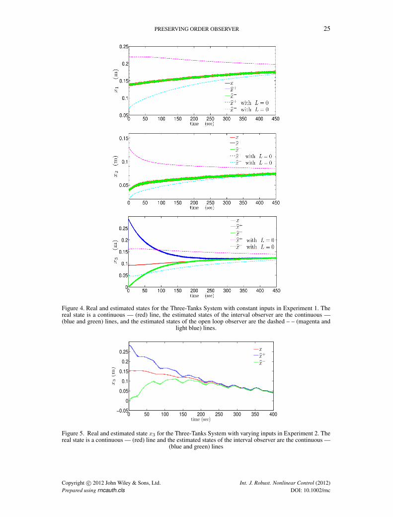
Experiment 2: For this test we consider the case without a leak in Tank 3. The input flowsare varying periodically asQ1(t) = 7.3284× 10−5 sin(0.1t) m3

s andQ2(t) = 1.9889× 10−5 m3

s . Theinitial conditions for the plant were x10 = 0.14 m, x20 = 0.04 m and x30 = 0.15 m, while the initialconditions for both observers are the same as in the previous Experiment 1.

Figure 5 shows the behavior of the real state x3 and its estimation by the interval observer underthese conditions. Note again that the estimated states are above/below their real values for all thetime, and that they converge (exponentially) to their true values.

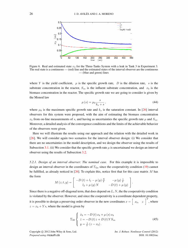
Experiment 3: For this test we consider the case with a leak in Tank 3. The input flows arekept constant, taking the same values as in Experiment 1. The initial conditions for the plantand the interval observer are also as in the previous Experiment 1. The bounds for the leak inthe third Tank is considered to be neither bigger than π+

3 = 3.5899× 10−6 m3

s nor smaller thanπ−3 = 1.5763× 10−6 m3

s , so that (22) holds.Figure 6 shows the behavior of the real state x3 and its estimation by the interval observer under

these conditions. Note that the estimated states are above/below their real values for all the time.However, in contrast to the nominal case considered in the two previous Experiments the estimationerror does not converge anymore to zero, but it converges (exponentially) to a final bound. Theestimated lower bound x−3 of the (unmeasured) level in Tank 3 can serve as an indicator when theTank will run empty, before it actually happens. Or the estimated upper bound x−3 of the same stateis an indicator of a possible overflow in the same tank.

5.2. A Stirred Tank Reactor

Consider a stirred tank reactor (STR) [26]:

Σ2a

xb = −D (t)xb + µ (s)xb

s = D (t) (Sin − s)− 1Y µ (s)xb

y = s

(43)



Figure 4. Real and estimated states for the Three-Tanks System with constant inputs in Experiment 1. Thereal state is a continuous — (red) line, the estimated states of the interval observer are the continuous —(blue and green) lines, and the estimated states of the open loop observer are the dashed – – (magenta and

light blue) lines.

0 50 100 150 200 250 300 350 400−0.05

0

0.05

0.1

0.15

0.2

0.25

time (sec)

x3(m

)

xx+

x−

Figure 5. Real and estimated state x3 for the Three-Tanks System with varying inputs in Experiment 2. Thereal state is a continuous — (red) line and the estimated states of the interval observer are the continuous —

(blue and green) lines



Figure 6. Real and estimated state x3 for the Three-Tanks System with a leak in Tank 3 in Experiment 3.The real state is a continuous — (red) line and the estimated states of the interval observer are the continuous

— (blue and green) lines

where Y is the yield coefficient, µ is the specific growth rate, D is the dilution rate, s is thesubstrate concentration in the reactor, Sin is the influent substrate concentration, and xb is thebiomass concentration in the reactor. The specific growth rate we are going to consider is given bythe Monod law

µ (s) = µ0s

ks + s, (44)

where µ0 is the maximum specific growth rate and ks is the saturation constant. In [26] intervalobservers for this system were proposed, with the aim of estimating the biomass concentrationxb from on-line measurements of s, and having as uncertainties the specific growth rate µ and Sin.Moreover, a detailed analysis of the convergence conditions and the limits of the achievable behaviorof the observers were given.

Here we will illustrate the results using our approach and the relation with the detailed work in[26]. We will consider again two scenarios for the interval observer design: (i) We consider thatthere are no uncertainties in the model description, and we design the observer using the results ofSubsection 3.1. (ii) We consider that the specific growth rate µ is uncertainand we design an intervalobserver using the results of Subsection 3.2.

5.2.1. Design of an interval observer: The nominal case. For this example it is impossible todesign an interval observer in the coordinates of Σ2a since the cooperativity condition (19) cannotbe fulfilled, as already noticed in [26]. To explain this, notice first that for this case matrix M hasthe form

M (z; t, y) =

[−D (t) + l1 − µ (y) NY −µ (y) 1

Y

l2 + µ (y)N −D (t) + µ (y)

].

Since there is a negative off-diagonal term, that does depend on L,N , the the cooperativity conditionis violated by the observer. However, and since the cooperativity is a coordinate dependent property,

it is possible to design a preserving order observer in the new coordinates x =[xb, z

]T, where

z = xb + Y s, where the model is given by

Σ2b

xb = −D (t)xb + µ (s)xb

z = −D (t) z +D (t)Y Sin

y = 1Y (z − xb) .

(45)



It is possible to write this (nominal) system in the form ΠS in (12) with matrices given by:

A =

[−D (t) 0

0 −D (t)

], G =

[0

1

],

H =[

0 1], C =

[1Y − 1

Y

].

The input/output injection vector ϕ (t, y, u), consisting of known signals affecting the dynamics ofthe plant, is given by

ϕ (t, y) =

[D (t)Y

0

]Sin (t) ,

and f (σ, y) = µ (y)σ. The incremental nonlinearity φ (σ, z) = µ (y)σ − µ (y) (σ + z) = −µ (y) z

is (Q, S, R)-D with (Q, S, R) = (−1,−0.5, 0), i.e. φ ∈ [−1, 0]. Convergence of the observer isguaranteed if the dissipativity inequality (18) is satisfied. For this case matrix M in (19) is

M (z; t, y) =

[−D (t) + l1

Y − l1Yl2Y + µ (y) NY −

(D (t) + l2

Y

)+ µ (y)

(1− N

Y

)],

so that the Cooperativity Condition is satisfied if l1 ≤ 0 and l2 + µ (y)N ≥ 0. When bothdissipativity (18) and cooperativity (19) inequalities are satisfied, so that Theorem 10 is satisfied,an interval observer of the form (23)-(24) can be designed, with the terms π+ = π− = 0. Note thatthis interval observer is similar to the one proposed by [26], except for two differences: (i) For theshake of the presentation, we have assumed that x− is always nonnegative, so that our observeris slightly simpler than the one in [26]. Our assumption is reasonable, and it is usually satisfied.(ii) Our interval observer has an extra injection term, N± (y± − y), entering in the nonlinearity.However, since the nonlinearity in this example is affine in the unmeasured state, i.e. µ (s)xb, thenthe estimation error is in fact linear time varying, and the injection term due to N becomes also alinear one, adding to the correction term with gain l2. Therefore, the extra correction term causesno qualitatively different behavior to the observer in [26] for this example. This will be clear in thesimulations below. We note, however, that our method generalizes the one proposed in [26].

Using the same parameters as in [26], i.e. ks = 5 g/l, Sin = 5 g/l, D = 0.05 h−1, µ0 = 0.33 h−1

and Y = 0.5, where D and Sin are constant, it is possible to find numerically (using e.g. thePENBMI software) that for the values

L =

[0

19.991

], N = −10 , P = 106

[7.8109 −0.0007

−0.0007 0.00004

], ε = 183.232

both inequalities (18) and (19) are satisfied. We select in interval observer N+ = N− = N andL+ = L− = L. Figure 7 shows the behavior of the interval observer. The initial conditions for theplant were xb0 = 1.05 g/l and s0 = 0.9 g/l, and those for the interval observer were set as

x+b (0) = 1.5 g/l , x−b (0) = 0 g/l,

z+ (0) = 0.45 g/l , z− (0) = 1.95 g/l .



As expected the estimation error preserves the order and it converges exponentially to zero. Asexplained in [26] the convergence velocity cannot be improved much further without violating thecooperativity condition.

0 50 1000

0.5

1

1.5

2

2.5

3

time t [h](a)

z[g/l]

0 50 1000

0.5

1

1.5

2

2.5

time t [h](b)

xb

[g/l]

0 50 100

−1

−0.5

0

0.5

time t [h](c)

e− z

e+ z

0 50 100

−1

−0.5

0

0.5

time t [h](d)

e− xb

e+ xb

Figure 7. Simulation of the bioreactor (−.), the estimation of the proposed interval observer (−) and theirestimation errors for the nominal case.

5.2.2. Interval observer design for the stirred tank reactor with uncertainties We consider now thatthe specific growth rate µ in (44) is uncertain, and known to be between lower and upper bounds

µ− (s) ≤ µ (t, s) ≤ µ+ (s) .

In particular, we assume that µ± (s) are given by Monod models (44) with µ+0 = 0.495 h−1 and

µ−0 = 0.165 h−1. The interval observer is of the form (23)-(24), where the terms π+ and π− aregiven by

π+ (t, y) = 0.165y

ks + yx+b , π

− (t, y) = −0.165y

ks + yx−b .

Using the same parameters as in the previous paragraph we found numerically a different set ofparameters satisfying both inequalities (18) and (19)

L =

[−0.5847

561.2413

], N = −10 , P = 104

[4.2090 −0.0025

−0.0025 0.0068

], ε = 506.6 .

We also select in interval observer N+ = N− = N and L+ = L− = L. For comparison we designalso the interval observer proposed in [26], that corresponds to the structure given by (23)-(24) withl1 = 0, l2 = 2.255, and N = 0. Figure 8 shows the behavior of the trajectories for the plant, both



0 50 1000

0.5

1

1.5

2

2.5

3

time t [h](a)

z[g/l]

0 50 1000

0.5

1

1.5

2

2.5

time t [h](b)

xb

[g/l]

0 50 100

−1

−0.5

0

0.5

time t [h](c)

e− z

e+ z

0 50 100

−1

−0.5

0

0.5

time t [h](d)

e− xb

e+ xb

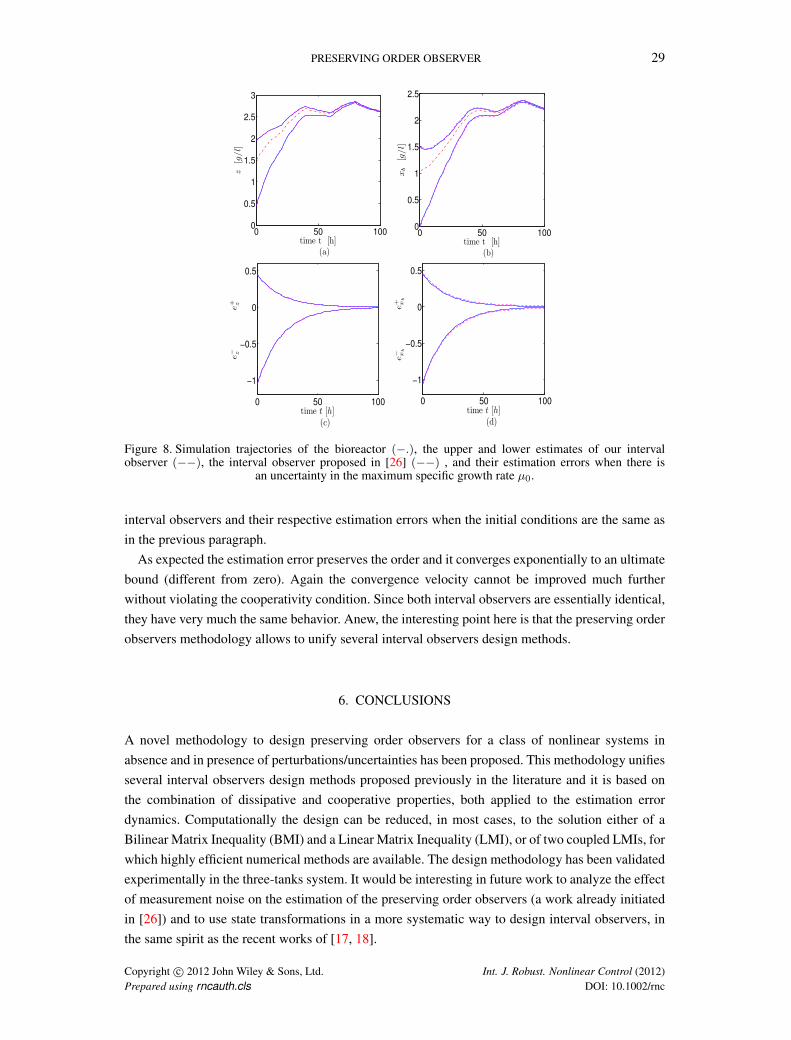
Figure 8. Simulation trajectories of the bioreactor (−.), the upper and lower estimates of our intervalobserver (−−), the interval observer proposed in [26] (−−) , and their estimation errors when there is

an uncertainty in the maximum specific growth rate µ0.

interval observers and their respective estimation errors when the initial conditions are the same asin the previous paragraph.

As expected the estimation error preserves the order and it converges exponentially to an ultimatebound (different from zero). Again the convergence velocity cannot be improved much furtherwithout violating the cooperativity condition. Since both interval observers are essentially identical,they have very much the same behavior. Anew, the interesting point here is that the preserving orderobservers methodology allows to unify several interval observers design methods.

6. CONCLUSIONS

A novel methodology to design preserving order observers for a class of nonlinear systems inabsence and in presence of perturbations/uncertainties has been proposed. This methodology unifiesseveral interval observers design methods proposed previously in the literature and it is based onthe combination of dissipative and cooperative properties, both applied to the estimation errordynamics. Computationally the design can be reduced, in most cases, to the solution either of aBilinear Matrix Inequality (BMI) and a Linear Matrix Inequality (LMI), or of two coupled LMIs, forwhich highly efficient numerical methods are available. The design methodology has been validatedexperimentally in the three-tanks system. It would be interesting in future work to analyze the effectof measurement noise on the estimation of the preserving order observers (a work already initiatedin [26]) and to use state transformations in a more systematic way to design interval observers, inthe same spirit as the recent works of [17, 18].



ACKNOWLEDGEMENT

The authors gratefully acknowledge the financial support from Fondo de Colaboracion del II-FI, UNAM,IISGBAS-165-2011; Programa de Apoyo a Proyectos de Investigacion e Innovacion Tecnologica (PAPIIT),UNAM, grant IN111012, and CONACyT (Consejo Nacional de Ciencia y Tecnologıa), grant 51244.

REFERENCES

1. Alcaraz-Gonzalez V, Harmand J, Rapaport A, Steyer J, Gonzalez-Alvarez V, Pelayo-Ortiz C. 2002. Software sensorsfor highly uncertain WWTPS: a new approach based on interval observers. Water Res;(36): 2515.

2. Angeli D, Sontag ED. 2003. Monotone control systems. IEEE Transactions on Automatic Control. 48(10), 1684–1698.

3. M. Arcak and P. Kokotovic, “Nonlinear observers: a circle criterion design and robustness analysis,” Automatica,vol. 37, no. 12, pp. 1923–1930, 2001.

4. Aviles JD, Moreno JA. 2009. Cooperative observers for nonlinear systems. Joint 48th IEEE Conference on Decisionand Control and 28th Chinese Control Conference, Shanghai, China, 6125–6130.

5. Bastin G, Dochain D. 1990. On-line Estimation and Adaptive Control of Bioreactors. Vol. 1 of Process Measurementand Control. Elsevier. Amsterdam.

6. Bernard O, Gouze J. 2004. Closed loop observers bundle for uncertain biotechnological models. Journal of ProcessControl 14(3), 765-774.

7. Boyd SP, El Ghaoui E, Balakrishnan V. 1994. Linear Matrix Inequalities in System and Control Theory. SIAM.Philadelphia.

8. Brogliato B, Lozano R, Maschke B, Egeland O. 2007. Dissipative systems analysis and control: Theory andapplications. (Second edn.) Springer.

9. Dochain D, Perrier M, Ydstie B. 1992. Asymptotic observers for stirred tank reactors. Chem. Eng. Sci., 47: 4167.10. J.-P. Gauthier, H. Hammouri, and S. Othman. A simple observer for nonlinear systems. Applications to bioreactors.

IEEE Trans. Automatic Control, 37:875–880, 1992.11. El Ghaoui L, Niculescu SI. 1999. Advances in Linear Matrix Inequality Methods in Control. SIAM. Philadelphia.12. Gouze JL, Rapaport A, Hadj-Sadok MZ. 2000. Interval observers for uncertain biological systems. Ecol Modelling,

133(1-2):45–56.13. Grunbaum B. 2003. Convex polytopes (second edn.) Springer. Seattle, USA.14. Hirsch MW, Smith HL. 2005. Handbook of differential equations: ordinary differential equations. Vol II. Elsevier

B.V. Amsterdam, 239–357.15. Khalil HK. 2002. Nonlinear Systems (third edn.) Prentice–Hall. Upsaddle River, New Jersey.16. Kocvara M, Stingl M. 2003. Pennon. A code for convex nonlinear and semidefinite programming. Methods and

Software. 18: 317–333.17. Mazenc F., Bernard O. Feb. 2010. Asymptotically Stable Interval Observers for Planar systems with Complex Poles.

IEEE Trans. on Aut. Control, vol. 55, Issue 2, pp. 523-527.18. Mazenc F, Bernard O. 2011. Interval observers for linear time-invariant systems with disturbances. Automatica.

47: 140–147.19. Moisan M, Bernard O, Gouze J. 2009. Near optimal interval observers bundle for uncertain bioreactors.

Automatica. 45: 291–295.20. Moisan M, Bernard O. 2010. Robust interval observers for global Lipschitz uncertain chaotic systems. Systems &

Control Letters. 59: 687–694.21. Moreno JA. 2004. Observer design for nonlinear systems: A dissipative approach. In: Proceedings of the 2nd IFAC

Symposium on System, Structure and Control SSSC2004. IFAC. Oaxaca, Mexico, Dec. 2004; 735–740.22. Moreno JA. 2005. Approximate observer error linearization by dissipativity methods. In: T. Meurer, K. Graichen

and E.D. Gilles (Eds.). Control and observer design for nonlinear finite and Infinite dimensional systems. Berlin,Springer-Verlag, 2005. Lecture Notes in Control and Information Sciences, 322 pp. 35-51.

23. Moreno, J.A. 2006 A Separation Property of Dissipative Observers for Nonlinear Systems. Proceedings of the 45thIEEE Conference on Decision and Control (CDC2006), San Diego, CA, USA, 13-15 Dec. 2006. pp. 1647-1652.

24. R. Rajamani. Observers for Lipschitz nonlinear systems. IEEE Trans. Automatic Control, 43:397–401, 1998.25. Rapaport A. and Gouze J.-L. 2003. Parallelotopic and practical observers for nonlinear uncertain systems. Int.

Journal. Control, 76(3):237–251.



26. Rapaport A, Dochain D. 2005. Interval observers for biochemical processes with uncertain kinetics and inputs.Mathematical Biosciences. (192): 235–253.

27. Rocha-Cozatl E, Moreno JA. 2010. Dissipative design of unknown input observers for systems with sectornonlinearities. International Journal of Robust and Nonlinear Control. 21(14):1623-1644.

28. Smith H.L. 1995. Monotone dynamical systems: An introduction to the theory of competitive and cooperativesystems. American Mathematical Society., vol. 75, 1995.

29. Tuan HD, Apkarian P. 2000. Low nonconvexity-rank bilinear matrix inequalities: Algorithms and applications inrobust controller and structure designs. IEEE Trans. on Automatic Control. Philadelphia. 11(45):2111–2117.

30. Vidyasagar M. 2002. Nonlinear systems analysis. (second edn.) SIAM. Englewood Cliffs, NJ.31. Willems JC. 1972. Dissipative dynamical systems, part I: General theory. Archive for Rational Mechanics and

Analysis 45, 321–351.32. Willems JC. 1972. Dissipative dynamical systems, part II: Linear systems with quadratic supply rates. Archive for

Rational Mechanics and Analysis 45, 352–393.


Preserving order observers for nonlinear systems · Interval observers, which consist of a couple...

Documents

Transcript of Preserving order observers for nonlinear systems · Interval observers, which consist of a couple...