Workshop 15

Single Pass Rolling of a Thick Plate

Introduction Rolling is a basic manufacturing technique used to transform preformed shapes into a form suitable for further processing. The rolling process is essentially quasi-static because rolling is normally performed at relatively low speeds (typically 1 m/s) and, therefore, inertia effects are not significant.

Representative rolling geometries generally require three-dimensional modeling, resulting in very large models, and include both nonlinear material behavior and nonlinear boundary effects (contact and friction). For this reason the explicit dynamics approach is often less expensive computationally and more reliable than an implicit quasi-static solution if mass scaling is used.

This workshop involves simulating quasi-static rolling of a plate using ABAQUS/Explicit. The rolling process reduces the thickness of the plate by 42% in a single rolling pass. Mass scaling will be used to reduce the solution time for analysis. For the purpose of comparison, the simulation will also be performed using the implicit solver available with ABAQUS/Standard.

This workshop is based in part on “Rolling of thick plates,” Section 1.3.6 of the ABAQUS Example Problems Manual.

Geometry and model A half-symmetry plane strain model will be used with the plate having a length of 0.092 m and a half-thickness of 0.02 m. A 90 segment of the roller is constructed as an analytical rigid surface.

1. Start a new session of ABAQUS/CAE from the ../IntroClass/workshops/rolling directory and create a new database.

A default model name is assigned by ABAQUS/CAE (Model-1). However, since the explicit dynamics model will later form the basis of the implicit analysis model, you should rename the current model to give it a more descriptive name.

2. In the Model Tree, click mouse button 3 on Model-1 and select Rename from the menu that appears. Rename the model Explicit.

3. In the Model Tree, double-click Parts to create a new part. Name the part plate,choose 2D Planar as the modeling space, and set the approximate size of the sketch area to 0.5. Review the other defaults, and click Continue.

W15.2

4. Using the Create Lines: Rectangle tool, sketch a rectangle 0.092 m long and 0.020 m high, as shown in Figure W15–1.

Figure W15–1 Plate geometry.

5. In the Model Tree, double-click Parts to create another part. Name the part roller. Choose the 2D Planar modeling space and the Analytical rigid part type. Set the approximate size of the sketch area to 2.0, and click Continue.

6. Using the Create Isolated Point tool, create two points with the coordinates(-0.170, 0.170) and (0, 0.170).

7. Using the Create Arc tool, sketch a 90 arc centered at the point (0, 0.170), as shown in Figure W15–2.

Figure W15–2 Roller geometry.

8. From the main menu bar, select Tools Reference Point and choose the center of the arc to create a reference point for the part.

W15.3

Materials and section The steel plate is assumed to be elastic-plastic. Although rate-dependent plastic behavior is usually considered in rolling simulations, it is not considered here.

1. In the Model Tree, double-click Materials. Create a material named Steel withthe following properties:

Modulus of elasticity: 1.5E11 Pa Poisson's ratio: 0.3

Density: 7850 kg/m3

The initial yield stress is 168.72 MPa rising to 448.45 MPa at 100% strain. Use the plasticity data provided in Table W15–1:

Yield stress (Pa) Plastic strain 1.6872 E8 0.0 2.1933 E8 0.1 2.7202 E8 0.2 3.0853 E8 0.3 3.3737 E8 0.4 3.6158 E8 0.5 3.8265 E8 0.6 4.0142 E8 0.7 4.1842 E8 0.8 4.3401 E8 0.9 4.4845 E8 1.0

Table W15–1 Yield stress-plastic strain data.

2. In the Model Tree, double-click Sections and create a homogeneous solid section named plateSection with the default thickness of 1.0.

3. In the Model Tree, expand the plate item underneath the Parts container and double-click Section Assignments in the list that appears. Assign plateSection to the part.

Assembly You must now instance the parts and position the plate relative to the roller.

1. In the Model Tree, expand the Assembly container and double-click Instances.2. In the Create Instance dialog box, select both parts and click OK.

To position the plate relative to the roller, it is necessary to identify the location on the roller where contact will first occur between the parts. Then datum geometry can be used to facilitate the positioning. In this problem the top-right corner of the plate will first make contact with the roller at a point that is located approximately 20% of the distance along the edge of the roller (relative to the bottom vertex of the roller).

W15.4

3. From the main menu bar, select Tools Datum to define a datum point using the Enter parameter method. Create the point on the roller edge, and specify a normalized edge parameter of 0.2.

4. From the main menu bar, select Instance Translate to modify the position of the plate. Define the translation vector using the start and end points shown in Figure W15–3.

Figure W15–3 Part positioning.

Sets and surfaces To facilitate the application of loads, contact, etc., you will create geometry sets and surfaces.

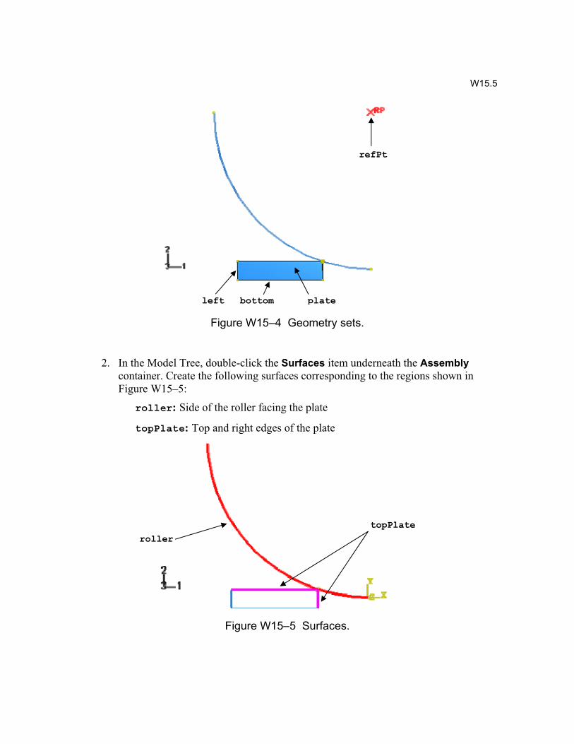
1. In the Model Tree, double-click the Sets item underneath the Assemblycontainer. Create the following sets corresponding to the regions shown in Figure W15–4:

left: The left edge of the plate

bottom: The bottom edge of the plate

plate: The entire plate

refPt: The reference point of the roller

end point start point

W15.5

Figure W15–4 Geometry sets.

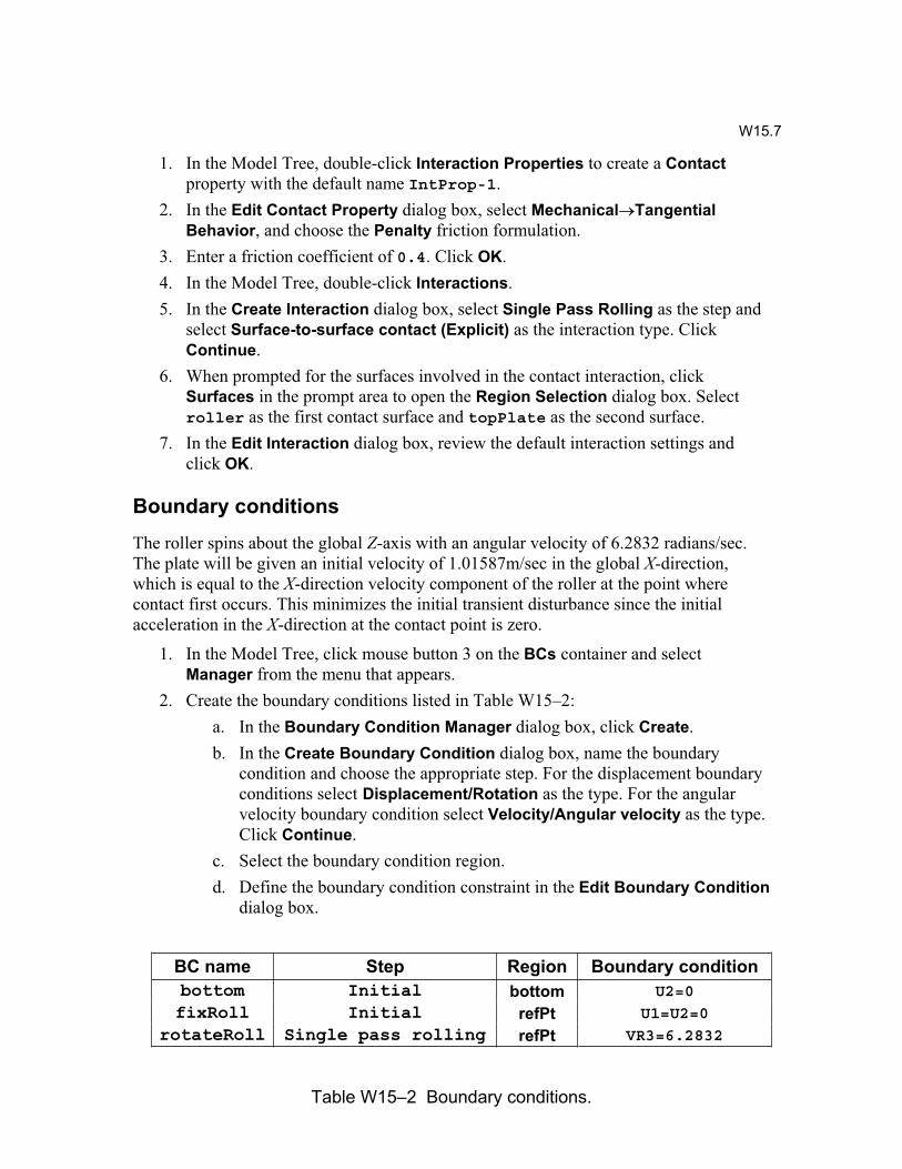
2. In the Model Tree, double-click the Surfaces item underneath the Assemblycontainer. Create the following surfaces corresponding to the regions shown in Figure W15–5:

roller: Side of the roller facing the plate

topPlate: Top and right edges of the plate

Figure W15–5 Surfaces.

left bottom plate

refPt

topPlateroller

W15.6

Analysis step and output requests The rolling simulation will be performed using a single explicit dynamics analysis step.

1. In the Model Tree, double-click Steps to create a Dynamic, Explicit step named Single Pass Rolling with a time period of 0.1 seconds. Accept all defaults for the time incrementation and other parameters.

Because rate effects are usually considered in rolling problems, the only method available to speed up the simulation effectively is mass scaling.

2. Open the Mass Scaling tabbed page of the Edit Step dialog box. In this page, select Use scaling definitions below then click Create.

3. In the Edit mass scaling dialog box, choose Set as the application region; and from the pull down menu, select plate. Enter a Scale by factor value of 1600.Click OK in the Edit mass scaling and Edit Step dialog boxes.

4. Accept the default field output requests. In the Model Tree, double-click History Output Requests to create a history output request for the reaction moment at the roller reference point. In the Edit History Output Request dialog box:

Select Set in the Domain field and select refPt from the list of sets that appears.Request stored history output at 100 equally spaced time intervals during the analysis. From the list of available output variables, click the arrows next to Forces/Reactions and RF, Reaction forces and moments to expand the variable lists. Toggle on RM3.Click OK.

Very large deformations are anticipated in this analysis. Use the adaptive meshing capability available in ABAQUS/Explicit to reduce the amount of mesh distortion and maintain a high quality mesh throughout the analysis.

5. From the main menu bar, select Other Adaptive Mesh Domain Manager.a. In the Adaptive Mesh Domain Manager, click Edit.b. In the Edit Adaptive Mesh Domain dialog box, toggle on Use the

adaptive mesh domain below. Select plate as the region. Specify a frequency of 10 and 3 mesh sweeps per increment.

c. Toggle on Adaptive mesh controls, and click Create in the right side of the dialog box. Define adaptive mesh controls using all supplied default parameters.

ContactSurface-to-surface contact will be defined between the top surface of the plate and the outer surface of the roller. Coulomb friction with a coefficient of 0.4 will be used.

W15.7

1. In the Model Tree, double-click Interaction Properties to create a Contactproperty with the default name IntProp-1.

2. In the Edit Contact Property dialog box, select Mechanical Tangential Behavior, and choose the Penalty friction formulation.

3. Enter a friction coefficient of 0.4. Click OK.4. In the Model Tree, double-click Interactions.5. In the Create Interaction dialog box, select Single Pass Rolling as the step and

select Surface-to-surface contact (Explicit) as the interaction type. Click Continue.

6. When prompted for the surfaces involved in the contact interaction, click Surfaces in the prompt area to open the Region Selection dialog box. Select roller as the first contact surface and topPlate as the second surface.

7. In the Edit Interaction dialog box, review the default interaction settings and click OK.

Boundary conditions The roller spins about the global Z-axis with an angular velocity of 6.2832 radians/sec. The plate will be given an initial velocity of 1.01587m/sec in the global X-direction,which is equal to the X-direction velocity component of the roller at the point where contact first occurs. This minimizes the initial transient disturbance since the initial acceleration in the X-direction at the contact point is zero.

1. In the Model Tree, click mouse button 3 on the BCs container and select Manager from the menu that appears.

2. Create the boundary conditions listed in Table W15–2: a. In the Boundary Condition Manager dialog box, click Create.b. In the Create Boundary Condition dialog box, name the boundary

condition and choose the appropriate step. For the displacement boundary conditions select Displacement/Rotation as the type. For the angular velocity boundary condition select Velocity/Angular velocity as the type. Click Continue.

c. Select the boundary condition region. d. Define the boundary condition constraint in the Edit Boundary Condition

dialog box.

BC name Step Region Boundary condition bottom Initial bottom U2=0

fixRoll Initial refPt U1=U2=0

rotateRoll Single pass rolling refPt VR3=6.2832

Table W15–2 Boundary conditions.

W15.8

Initial conditions As mentioned earlier, the plate is given an initial velocity of 1.01587 m/sec in the global X-direction.

1. In the Model Tree, double-click Fields.2. In the Create Field dialog box, select the Initial step, the Mechanical category,

and the Velocity type. Name the field initVel and click Continue.3. Select the set plate as the region for the initial velocity field.4. In the Edit Field box, enter a value of 1.01587 m/sec for the velocity component

V1.

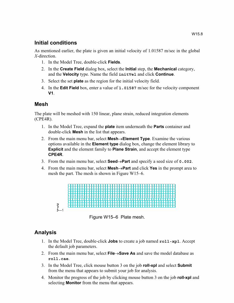
MeshThe plate will be meshed with 150 linear, plane strain, reduced integration elements (CPE4R).

1. In the Model Tree, expand the plate item underneath the Parts container and double-click Mesh in the list that appears.

2. From the main menu bar, select Mesh Element Type. Examine the various options available in the Element type dialog box, change the element library to Explicit and the element family to Plane Strain, and accept the element type CPE4R.

3. From the main menu bar, select Seed Part and specify a seed size of 0.002.4. From the main menu bar, select Mesh Part and click Yes in the prompt area to

mesh the part. The mesh is shown in Figure W15–6.

Figure W15–6 Plate mesh.

Analysis 1. In the Model Tree, double-click Jobs to create a job named roll-xpl. Accept

the default job parameters. 2. From the main menu bar, select File Save As and save the model database as

roll.cae.3. In the Model Tree, click mouse button 3 on the job roll-xpl and select Submit

from the menu that appears to submit your job for analysis. 4. Monitor the progress of the job by clicking mouse button 3 on the job roll-xpl and

selecting Monitor from the menu that appears.

W15.9

Visualization1. Once the analysis completes successfully, click mouse button 3 on the job roll-xpl

in the Model Tree and select Results from the menu that appears. 2. Plot the undeformed and the deformed model shapes. 3. From the main menu bar, select View ODB Display Options.4. In the ODB Display Options dialog box, choose the Extra Fine curve refinement

level. Click the Sweep and Extrude tab and set the extrusion depth to 0.01.Click OK.

5. Turn on shaded render style, and rotate the model. 6. Plot the contours for MISES stress and plastic strain PEEQ. The contours for

Mises stress are show in Figure W15–7.

Figure W15–7 Mises stress contours.

7. From the main menu bar, select Animate Time History to animate the history of the Mises stress distribution and the resulting deformation.

8. From the main menu bar, select Result History output to create X–Y plots for the model kinetic energy (ALLKE), external work (ALLWK), internal energy (ALLIE), and total energy (ETOTAL). In the History Output dialog box, click Plot to display the curves and click Dismiss to close the box. The plot is shown in Figure W15–8.

W15.10

Figure W15–8 Model energies.

9. Plot the history of the reaction moment RM3, and save the curve as RM3 XPL.

Implicit analysis model Now perform the simulation using ABAQUS/Standard. You will copy the model for the ABAQUS/Explicit analysis and modify the new model as described below.

1. In the Model Tree, click mouse button 3 on the model Explicit and select Copy Model from the menu that appears. In the Copy Model dialog box, name the new model Standard. Click OK.

2. Replace the Single Pass Rolling step with a Static, General step.

For the implicit analysis, the static analysis procedure will be used. Note, however, that the simple analysis technique used earlier (whereby the initial plate velocity was prescribed and a single analysis step was used) will not yield the desired results in ABAQUS/Standard. The reason is that, in a static step material inertia is neglected. Thus, two steps are needed to perform the simulation. In the first step firm contact must be established between the plate and the roller. This then allows the roller to draw the plate in the second step, where the roll pass event will be simulated.

The adaptive meshing capability in ABAQUS/Standard is not intended to be used for general large-deformation problems, such as bulk metal forming. Deactivate adaptive meshing for this step as follows:

W15.11

3. From the main menu bar, select Other Adaptive mesh domain EditEstablish Contact to edit the adaptive mesh domain for this step.

4. In the Edit Adaptive Meshing Domain dialog box, choose No adaptive mesh domain for this step and click OK.

5. Rename the step Establish Contact with the following parameters: Total time period = 0.001 secMaximum number of increments = 100Initial time increment size = 0.0001 secMinimum increment size = 1E-8 secMaximum increment size = 0.001 secNLGEOM toggled on

6. Create a second Static, General named Roll Pass with the following parameters:

Total time period = 0.099 secMaximum number of increments = 500Initial time increment size = 0.0001 secMinimum increment size = 9.9E-7 secMaximum increment size = 0.099 sec

7. From the main menu bar, select Output Restart Requests and specify a restart frequency of 250 for each step.

8. Edit the field output requests so that preselected output is written every 25 increments during each analysis step.

For problems dominated by highly discontinuous nonlinearities (such as contact and friction), nondefault analysis controls may aid the convergence behavior. In this problem allow extra equilibrium iterations for the resolution of these discontinuities, as described below.

9. From the main menu bar, select Other General Solution Controls EditRoll Pass to edit the solution controls for this step.

10. In the solution controls editor, select Specify. In the Time Incrementationtabbed page of this dialog box, toggle on Discontinuous analysis. Click OK to close the dialog box.

11. In the Model Tree, double-click BCs to create the Velocity/Angular velocitytype boundary condition listed in Table W15–3.

BC name Step Region Boundary conditionfeed piece Establish Contact left V1=1.01587

Table W15–3 New boundary condition.

W15.12

12. In the Model Tree, click mouse button 3 on the BCs container and select Manager from the menu that appears.

13. In the Boundary Condition Manager dialog box, select cell for the feed pieceboundary condition in the Roll Pass step, and click Deactivate.

14. In the Model Tree, expand the plate item underneath the Parts container and double-click Mesh in the list that appears.

15. From the main menu bar, select Mesh Element Type; and, in the Element typedialog box, change the element library to Standard and click OK.

16. Save the model database. 17. Create a job named roll-std for the model Standard.18. Submit the job for analysis. 19. Monitor the progress of the job by clicking mouse button 3 on the roll-std item

underneath the Jobs container and selecting Monitor in the menu that appears.

Visualization1. Once the analysis completes successfully, click mouse button 3 on the job roll-std

in the Model Tree and select Results in the menu that appears. 2. Plot the undeformed and the deformed model shapes. 3. Plot the contours for MISES stress and plastic strain PEEQ.4. Create a second viewport by selecting Viewport Create from the main menu

bar. Tile the viewports horizontally (Viewport Tile Horizontally).5. Switch to the output database file roll-xpl.odb, and plot the contours for

PEEQ. The contours for PEEQ for both analyses are shown in Figure W15–9.

W15.13

Figure W15–9 PEEQ for the implicit and explicit solutions.

6. Save the time history for the reaction moment RM3 as RM3 STD. Plot both curves as shown in Figure W15–10.

Figure W15–10 Comparison of the reaction moment history.

Note: A script that creates the complete model described in these instructions is available for your convenience. Run this script if you encounter difficulties following the instructions outlined here or if you wish to check your work. The script is named ws_intro_rolling.py and is available using the ABAQUS fetch utility.

explicit solution

implicit solution