Present Value and the Commercial Property Price

Present Value and the Commercial Property Price∗

－ New Estimation Methods of the CPPI using J-REIT data－

Chihiro Shimizu† ,W. Erwin Diewert‡ ,Kiyohiko.G. Nishimura§ ,Tsutomu Watanabe¶

Nov 15, 2012

Abstract

While fluctuations in commercial property prices have an enormous impact on eco-nomic systems, the development of related statistics that can capture these fluctuationsis one of the areas that is lagging the furthest behind. The reasons for this are that,in comparison to housing, commercial property has a high level of heterogeneity andthere are extremely significant data limitations. Focusing on the Tokyo office market,this study estimated commercial property price indexes using the data available in theproperty market, and clarified discrepancies in commercial property price indexes basedon differences in the method used to create them. Specifically, we estimated a quality-adjusted price index with the hedonic price method using property appraisal pricesand transaction prices available for the J-REIT market. In addition, we attemptedto estimate a price index based on a present value model using revenues arising fromproperty and discount rates. Here, along with the discount rates underlying the de-termination of property appraisal prices and transaction prices, we obtained discountrates using enterprise values that can be acquired from the J-REIT investment market,and estimated the respective risk premiums. First, the findings showed that, comparedto risk premiums formed by the stock market, risk premiums when determining prop-erty appraisal prices change only relatively gradually, with the adjustment speed beingespecially slow while the market is contracting. As a result, these prices decline onlyslowly. They also showed that until the Lehman Shock, property market risk premi-ums formed by the stock market were at a lower level than risk premiums set whendetermining property appraisal prices and transaction prices, but following the LehmanShock, the respective risk premiums converged toward the same level.

Key Words :quality adjusted price index; hedonic approach; discout rate; hetero-geneity; Tobin’s q; Risk premium

JEL Classification : E3; G19

∗In order to prepare this paper, data was supplied by Nikkei Digital Media Inc. As well, MinoruKato, Toshiro Nishioka, Toshihiro Doi, Naoto Otsuka and Yasuhito Kawamura collaborated on organiz-ing/analyzing the data. We would like to hereby express our gratitude to them. Nishimura’s contributionwas made mostly before he joined the Policy Board. In addition, this study received JSPS Grant-in-Aid forScientific Research B (No. 23330084).”

†Correspondence: Chihiro Shimizu, Reitaku University & The University of British Columbia, Kashiwa,Chiba 277-8686, Japan. E-mail: [email protected].

‡The University of British Columbia§The deputy Governor of Bank of Japan¶The University of Tokyo

1

1 Introduction

Looking back at the history of economic crises, there are more than a few cases wherea crisis was triggered by the collapse of asset market prices. It is recognized that thecollapse of Japan’s 1980s’ land/stock price bubble in the early 1990s was closely relatedto the subsequent economic stagnation, and in particular the banking crisis that startedin the latter half of the 1990s. Moreover, the 1990s’ crisis in Scandinavia also occurred intandem with a property bubble collapse. The global financial crisis that began in the U.S.in 2008 and the recent European debt crisis were triggered by the collapse of bubbles in theproperty and financial markets as well. Examples of bubble collapses becoming the triggerfor an economic crisis are not limited to advanced nations; it has been widely observed inemerging nations as well, such as Asian countries.

In this context, the importance of precisely capturing fluctuations in the property marketis widely recognized, and active efforts are being made to develop property price indexes1.However, when it comes to property price indexes, the body of research relating to non-housing assets – i.e., commercial property price indexes – is small, and the development ofsuch indexes is an area where both public institutions and the private sector are laggingbehind. There are thought to be several reasons for this, one of which is the difficulty ofestimating such indexes. This difficulty is due to the presence of the following problems:1) the highly heterogeneous nature of commercial property buildings, which have a diverserange of attributes (there is considerable variation in quality and in size attributes such asheight), and 2) the strong data limitations due to the transaction volume being extremelysmall compared to general assets and services or even other property such as housing.

As a result, there is an extremely high level of technical difficulty involved in preparingthese statistics, and the cost of producing data is high.

Looking first at commercial property-related statistics from public or quasi-public or-ganizations, there is Japan’s “Urban Land Price Indexes” – one of the oldest publishedcommercial property price indexes among advanced nations. Surveying for Urban LandPrice Indexes began on a trial basis in 1926, and from 1955 onward, indexes have beencreated covering 230 cities throughout Japan.2 What’s more, in Japan, a Land Price Surveycovering the whole country was initiated by the former National Land Agency (now theMinistry of Land, Infrastructure, Transport and Tourism) in 1970. Not only does the LandPrice Survey publish price levels by location for commercial land in addition to residentialand industrial land, its also publishes indexes comparing the rate of change to the sameperiod in the previous year. It is necessary to note, however, these indexes are not commer-cial property price indexes including buildings and land; rather, they are land price indexes

1With regard to property price indexes, the international Handbook on Residential Property Prices,which stipulates guidelines for creating housing price indexes, was published in 2011. It is available at:http://epp.eurostat.ec.europa.eu/portal/page/portal/hicp/methodology/owner occupied housing hpi/rppi handbook

2It has been prepared since 1926 when one includes the organization previously responsible for producingit. This index was created by Nippon Kangyo Bank, predecessor of the Japan Real Estate Institute. SinceNippon Kangyo Bank was a state-run bank, its index played the role of an official index. This surveypublished not only a commercial land price index but also a housing land price index and an industrial landprice index.

2

limited to land only .And, these indexes are appraisal basd indexes, not transaction basedindexes.

In Germany as well, federal and state statistical agencies have published a transactionprice index (Kaufwert fur Bauland) since 1961.3 However, this survey is a simple aggregateof land on which there has not yet been any construction, and the use to which it will be put– such as whether it will be built up as commercial property, developed as housing, or left asis without any construction – is unclear. In this sense, it cannot be treated as a commercialproperty price index in the strict meaning of the term.

With regard to this, in recent years, in tandem with the growth of the property investmentmarket, “property investment indexes” have come to be created by private-sector compa-nies/organizations. Leading indexes include the U.S. NCREIF and the index produced byIPD, a U.K.-based company. Moreover, in the U.S., the MIT/CRE Transaction Based In-dex (TBI) and Moody’s/REAL Commercial Property Price Index (CPPI) have come to bepublished.4 Compared to the Urban Land Price Indexes, Land Price Survey, and NCREIFand IPD land price indexes, which are appraisal-based property price indexes, these indexesare distinct in the sense they are based on transaction prices. In addition, they are qualityadjusted: the TBI based on the hedonic approach and the CPPI based on the repeat salesprice method.

Looking at the existing commercial property price indexes mentioned above, excludingthose indexes that started to be published recently such as the U.S. TBI and CPPI, one cansee that in most cases commercial property price indexes are appraisal-based.

One of the reasons for this may be that, as mentioned previously, commercial propertyhas a high level of heterogeneity, and due to the small transaction volume, it is difficult toapply the hedonic price method or repeat sales price method widely used for housing priceindexes. As well, if one considers the realities of property appraisal practice, when it comesto determining the appraisal value of a commercial property price, it is not a transactioncase comparison method that infers the value from the transaction prices of surroundingproperties; rather, in general, the focus is on the income capacity generated by the property,and the property appraisal price is determined based on an income approach that obtainsthe discounted cash flow for the income. In other words, the actual transaction price isnot used; instead, the focus is on income and the discount rate that converts income into apresent value.

This has some important implications in terms of estimating commercial property priceindexes. If the experience acquired in property appraisal practice is correct, when it comesto estimating commercial property price indexes, we should consider focusing not on thetransaction price but rather on the income generated by the property and the discount rate

3The transaction price index is implemented based on a land price survey stipulated in Article 2-5 andArticle 7 of a price statistics-related law (Gesetz uber die Preisstatistik) enacted in 1958. Each state’sstatistical agency began surveying transaction examples of building plots which had not yet been used forconstruction within municipal urban planning areas, and after conducting the survey on a trial basis in thethird quarter of 1961, the federal statistics agency has been publishing quarterly and annual building landprice statistics since 1962.

4Each of these indexes is created and published by MIT’s Center for Real Estate. Refer tohttp://mit.edu/cre/research/credl/rca.html for details.

3

that converts it into a present value.Taking the Tokyo office market as an example and using transaction prices and property

appraisal value information published for the REIT market, this paper proposes a new priceindex estimation method based on the income capitalization value indicated in propertyappraisals – i.e., a “present value model.”

When relying on a present value method, one faces the following two issues when deter-mining asset values: determining income, and determining the discount rate.

First, we focused on the issue of setting the discount rate.Published J-REIT information includes the net operating income (NOI) per property and

the property appraisal value determined by a property appraiser. Accordingly, using thesedata, we explicitly demonstrated the relationship between the price index using propertyappraisal value information, the NOI index, and the discount rate index, and we clarifiedits micro structure.

However, as has been demonstrated in many previous studies, the property appraisal valuedetermined by a property appraiser is known to diverge from the actual market conditions.It is therefore important to understand what kind of technical reason causes the propertyappraisal value determined by a property appraiser to diverge from the actual market con-ditions. First, since the NOI which serves as the numerator is an actual value, it is a fixedvariable that will not change regardless of which organization evaluates it. On the otherhand, the discount rate is a random variable with a certain probability distribution, whichmeans that there will be problems in setting this rate. Therefore, we broke down the discountrate into the factors that comprise it: the rate of return on risk-free assets, the anticipatedfuture growth rate, and the risk premium. Of these, the rate of return on risk-free assetsis observable since the rate of return on government bonds and the like is generally used,and it does not change significantly. It is also difficult to believe that the rate of increasein income or the income from property will fluctuate significantly. That being the case, itbecomes clear that the reason why property appraisal values diverge from market values isthat there is a problem in setting the risk premium. If that is so, the question is whether therisk premiums set by property appraisers are appropriate and, if they are not appropriate,how should they be set?

Accordingly, in this study, we focused on the setting of risk premiums. Specifically, weproposed a method of setting risk premiums that are forecast based on trends in REITshares evaluated on the stock market, which is said to be one of the most efficient markets,and estimated a new commercial property price index.

Next, there is the problem of determining net operating income (NOI). The NOI used inproperty appraisals and the like is calculated based on the actual paying rent. However,as Shimizu, Nishimura, and Watanabe (2012) have shown, a significant discrepancy existsbetween paying rent and market rent. Paying rent is heavily weighted toward ongoing rentbased on leases agreed in the past rather than new rental leases agreed at a given point intime (market rent). In that case, paying rent is not able to sufficiently reflect the marketconditions. In this paper, after estimating a rent index using only newly contracted market

4

rents, we also estimated an office price index when rent was converted into market rent.Section 2 first outlines issues in estimating commercial property price indexes as well as

previous research. Section 3 shows the estimation models along with the data. Section 4shows the limitations of estimating a hedonic-style commercial property index using priceinformation and the estimation results for a new commercial property price index based ona present value model. Finally, Section 5 outlines our conclusions.

2 Issues in Commercial Property Price Index Estima-

tion

2.1 Types of Commercial Property Price Indexes and Related Is-

sues

In this section, we will outline commercial property price index data sources and estimationmethods.

Japan’s Urban Land Price Indexes and Land Price Survey, the U.S. NCREIF, and theindex produced by the U.K.-based IPD are appraisal-based property price indexes. Amongthese, Japan’s Urban Land Price Indexes and Land Price Survey are appraisal-based prop-erty price indexes for land prices only, which do not include building prices. On the otherhand, the IPD and NCREIF indexes are appraisal-based property price indexes which also in-clude building prices. In contrast to these, the German property price index, Moody’s/REALCommercial Property Price Index (CPPI), and MIT commercial property index (TBI) aretransaction-based property price indexes.

Next, we will look at differences in estimation methods. When estimating property priceindexes, it is necessary to perform quality adjustment, as indicated in the Residential Prop-erty Price Index Handbook. Since properties have a high level of individuality, it is notpossible to assume the homogeneity of assets, which is a premise of index theory.

Since indexes created based on property appraisals are, as a general rule, fixed-point sur-veys of the same property, they are estimated based on straightforward averages (or weightedaverages). With regard to indexes using transaction prices, the German property price in-dex is created with straightforward average values without performing quality adjustment.In contrast, the Moody’s/REAL Commercial Property Price Index (CPPI) and MIT com-mercial property price index (TBI) are indexes for which quality adjustment is performed.The Moody’s/REAL Commercial Property Price Index (CPPI) is estimated based on therepeat sales price method and the MIT commercial property price index (TBI) based on thehedonic price method.5

If one looks at them from the perspective of quality adjustment, there are problemswith these indexes. First, with regard to the NCREIF and IPD indexes using propertyappraisals, the populations from which the data used to create the indexes is extracted

5Each of these indexes is created and published by MIT’s Center for Real Estate. Refer tohttp://mit.edu/cre/research/credl/rca.html for details.

5

changes on a continuous basis. Since the purpose of these indexes is to capture changesin property investment market investment values, they are estimated by taking investmentproperties as the population. As a result, if a given property is sold off and is no longer aninvestment target, it is removed from the index; if a property becomes a new investmenttarget, it becomes part of the index. In other words, the properties which are the targetsof index creation change continuously. In this case, although there is no problem in termsof measuring investment values, in the case of trying to capture changes in quality-adjustedprices, a bias occurs with the indexes.

Next, we will consider cases using transaction prices. First, if one tries to apply therepeat sales price method, there needs to be enough transactions to meet the prerequisites.However, when attempting to estimate commercial property price indexes, in many countriesit is often difficult to collect sufficient transaction price data. In addition, with the repeatsales price method, one also faces the depreciation problem and renovation problem (Diewert,2007; Shimizu, Nishimura, and Watanabe, 2010).

Problems likewise occur with the NCREIF and IPD indexes that use property appraisals.With regard to property appraisal prices, since prices are surveyed at different times, as abuilding ages, it will be evaluated at a lower price in accordance with its aging, while ifadditional investment is made; it will be evaluated at a higher price in accordance with thatinvestment. Both depreciation and increases/decreases in capital expenditure are factoredin.

Meanwhile, if one attempts to estimate using the hedonic price method, it is necessaryto collect considerable property price-related attribute data. Generally, when one tries tocollect commercial property transaction prices, it is collected based on registry information.Since registry information only includes the price, address, floor space, and transaction date,if one tries to collect property characteristics that include other building attributes, one canexpect that it will involve considerable time and expense.

In order to tackle these problems, Shimizu and Nishimura (2006, 2007) and Shimizu, Diew-ert, Nishimura, and Watanabe (2012) eliminated building prices from commercial propertytransaction prices and restricted themselves to land prices only, then estimated using the he-donic price method. In this case, since there is no longer any need to collect building-relatedcharacteristics, quality adjustment can be performed with land-related characteristics only.However, in this case, one is faced with the problem of how to eliminate building prices.

Meanwhile, the MIT commercial property price index (TBI) is estimated using the hedonicprice method using NCREIF data. The NCREIF data-set includes detailed data relatingto property appraisals. Since property-related characteristics (position, size, building age,transportation accessibility, etc.) are provided in the property appraisal data, it includesenough information to apply the hedonic method. Moreover, IPD, which has a similardatabase, also employs the hedonic method, and is moving forward with the developmentof a transaction price index (S. Devaney and R.M. Diaz, 2009).

However, with regard to using this kind of information, it can only be used in countrieswhere a property investment market exists and, in addition, the information is disclosed.

6

2.2 Previous Research

Many of the problems surrounding the estimation of commercial property price indexesare problems which are shared with residential property price index estimation. Many ofthese issues have been outlined in Diewert (2007) and the Residential Property Price Index(RPPI) Handbook.

However, in comparison to research relating to housing price index estimation, which hasemphasized estimation methods, research relating to commercial property price indexes hasemphasized problems in the selection of data for the purpose of creating indexes.6 In termsof differences from the housing market, two broad points have been outlined with regardto the commercial property market’s characteristics. The first is, compared to housing, thenumber of transactions in the commercial property market is extremely limited, meaning itis an extremely “thin” market. The second is, compared to housing, which is a relativelyhomogeneous market, the commercial property market is strongly heterogeneous.

In order to overcome these property price index-related characteristics (problems) in thecommercial property market, the focus has come to center on appraisal-based property priceindexes.7 Since property appraisal prices are not prices transacted on the market but ratherprices determined by property appraisers, they may diverge from the actual market condi-tions. As a result, various discussions have developed surrounding the precision/accuracy ofthese property appraisal prices.

Specifically, the following points have become issues of discussion: Are indexes based onproperty appraisal prices able to precisely capture market turning points? (The problem ofthere in fact being a lag has been pointed out; this is known as the “lagging problem.”) Doproperty appraisal prices diverge from market prices? (They in fact diverge considerably inperiods of market fluctuation; this is known as the “valuation error problem.”) Are theyable to precisely capture market volatility (the amount of risk)? (It has been reported thatthese values smooth out market changes; this is known as the “smoothing problem.”)

For example, Geltner, Graff, and Young (1994) have clarified the aggregation bias mech-anism in the NCREIF index, the leading U.S. appraisal-based property price index, whileGeltner and Goetzmann (2000) have estimated an index with transaction prices and clari-fied the extent of appraisal evaluation errors and smoothing for NCREIF property appraisalprices. These problems are not just problems with the NCREIF appraisal-based propertyindex: they relate to the creation of all appraisal-based property indexes, including IPD’s.

In addition, focusing on Japan’s bubble period, Nishimura and Shimizu (2003), Shimizuand Nishimura (2006, 2007), and Shimizu et al. (2012) estimated a transaction price index

6Problems surrounding the estimation of commercial property price indexes are comprehensively outlinedby Geltner and Pollakowski (2007). As well, problems surrounding data selection for the estimation ofhousing price indexes are addressed by Shimizu, Nishimura, and Watanabe (2011). Here, the focus is onthe relationship between offer prices and transaction prices. Data source problems surrounding commercialproperty relate to the selection of property appraisal prices and transaction prices.

7For housing price index estimation as well, indexes using property appraisal values are estimated withthe SPAR (Sale Price Appraisal Ratio method). However, since they are used in combination with transac-tion prices, no significant discussion has arisen regarding the precision/accuracy or characteristics of propertyappraisal values.

7

for commercial property and housing and a hedonic price index for appraisal prices, andstatistically clarified the differences between the two. Looking at the estimation resultsmade it clear that during the bubble period, when there was an especially large increasein property prices, appraisal-based property price indexes could not sufficiently keep pacewith transaction prices, and they also could not keep up with the rate of decline duringthe period when prices dropped. For commercial property prices, the results showed thatbecause property prices increased at a rapid rate in the bubble period, property appraisalprices at the bubble’s peak were only able to reach 60% of transaction prices at the bubble’speak. As well, it was shown that they could not keep pace with the rate of decline during thebubble’s collapse, remaining at a level approximately 20% higher than transaction prices.

Much research has also been conducted that attempts to elucidate the mechanisms causingthe likes of the lagging problem, valuation error problem, and smoothing problem (Shimizuet al., 2012).

Quan and Quigley (1991) and Clayton et al. (2001) are examples of studies that attemptedto clarify the micro structure of these problems. They have shown that due to the lag indata acquired by property appraisers, the data selection method, and the existence of a lagmechanism until a decision is made, property appraisal prices have a structural smoothingproblem.8 As well, property appraisals for investment properties involve an additional sys-temic factor: the problem of interference from the client. This problem differs in naturefrom the problem of property valuation errors or the smoothing problem. Specifically, it is aproblem involving the property appraisal client inducing the property appraiser to raise theprice in an attempt to maintain the property’s investment performance (Crosby et al., 2003;Crosby, Lizieri, and McAllister, 2009). As a result of these inherent property appraisal tech-nical and systemic factors, property appraisal prices end up diverging from actual marketconditions.

Given this, efforts have been made to clarify the property price fluctuation mechanismand level of smoothing using data such as property equity determined by the stock marketand price (share value) of investments in real estate investment trusts (Fisher, Geltner, andWebb, 1994; Geltner, 1997).

Moreover, attempts have also been made to create commercial property price indexes usingactual transaction prices. In terms of methods of estimating quality-adjusted property priceindexes using transaction prices, the hedonic price method and repeat sales price method arethe leading estimation methods. In the case of attempting to estimate a price index usingthe hedonic price method, considerable property-related characteristic data is needed. Sincecommercial property in particular has a high level of heterogeneity, many more variablesare needed in comparison to housing, etc.9 Fisher et al. (2003) and Fisher, Geltner, and

8This problem is also outlined in Shimizu et al. (2012). With regard to the selection of transactioncomparables when the property appraiser is determining the price, there is a strong possibility that examplesthat diverge significantly from past conditions will be treated as outliers. If prices diverge from marketfluctuations as a result, there will be a lag. This problem is equivalent to problems in the creation ofconsumer price indexes, such as the selection of survey stores and products, the handling of sales, etc.

9As pointed out by Ekeland, Heckman, and Nesheim (2004), in hedonic function estimation, if explana-tory variables are lacking, the index estimation-related problem known as omitted variables bias will occur.

8

Pollakowski (2007) have estimated transaction price indexes based on the hedonic methodusing NCREIF transaction price data. This is because the NCREIF database providesproperty characteristic-related data, since it includes property appraisal price-related data.Geltner and Goetzmann (2000) have estimated a transaction price index based on the repeatsales price method using transaction price data.

When attempting to estimate transaction price indexes using these kinds of methods,since the commercial property market is a thin market in terms of transactions, besides theproblem of applicable methods, the problems of spatial aggregation unit (can the index beestimated for the whole country or by region?) and estimation frequency (is an annual,quarterly, or monthly index possible?) have also become significant points of discussion(Bokhari and Geltner, 2010).

3 Data and Estimation Model

3.1 Data10

As can be understood from previous research, the main points of discussion regardingcommercial property price indexes are what kind of biases exist with appraisal-based prop-erty price indexes (which are used for most commercial property price indexes) and whatestimation method is preferable in terms of quality adjustment.

In this study, we will estimate a commercial property price index using published J-REITmarket data for the Tokyo-area office market. This data includes the transaction price (V T )when an investment company listed on the J-REIT market makes a purchase or sale andthe property appraisal price(V A) evaluated once every six months.

In addition, along with property appraisal prices, we calculated rental income (Y A),corresponding expenses such as property tax and damage insurance premiums (O), and netincome after expenses (yA=Y A-O : Net Operating Income).11

In terms of property-related characteristic data, land area (L : m2), floor space of building(S : m2), rentable floor space representing a source of income (RS : m2)12 Cage of building(A: years), number of stories (H : number of stories), nearest station and time required toreach it (TS : minutes), leasehold format (LHD : right of ownership, standard leasehold, orfixed-term leasehold), and so forth are surveyed by property appraisers.13 In addition, since

10With regard to the data used in this study, the Nikkei Inc.’s R-Square was used. Nikkei Digital Mediaand Sound-F collaborated in supplying the data.

11In published information on J-REITs, taxes and public dues for the year the property is acquired arenot recorded as expenses in order to balance taxes and public dues paid when the property is acquired.Accordingly, in the data-set used in this analysis, we obtained the actual value of taxes and public dues fromaccounting data for the year following the property’s acquisition, and calculated NOI by using this data asa substitute for the taxes and public dues in the year the property was acquired.

12Rentable floor space refers to the amount of the building floor space within the transaction targetbuilding that represents a source of generating income. Shared areas such as the entrance and areas of thebuilding which were not covered by the transaction are eliminated from this.

13These property characteristics are surveyed by property appraisers for the purpose of performing prop-erty appraisal. Building-related data is surveyed separately in the form of building engineering reports byresearch organizations aimed at architects and the like.

9

the nearest station is surveyed, we added the average day-time travel time to the centralbusiness district (Tokyo Station) using train network data (TT : minutes).14

This data may be considered as having the same characteristics as U.S. NCREIF or U.K.IPD data. An overview of the data is provided in Table1.

3.2 Theoretical Framework

If one follows traditional economic theory, property prices may be determined as thediscounted cash flow of income generated from property. Based on this type of economictheory, there are two broad methods of estimating property price indexes.

The first method is to estimate the index using data on property prices transacted on themarket. Attempts to estimate property price indexes based on this kind of method havebeen reported in many studies focusing on housing price indexes and the like.

The second method is to obtain the discounted cash flow of income generated by property.This kind of value is known as the fundamental value and is based on basic capital theoryformulae.

Here,V tv is the initial asset value for the period t, for which v years have elapsed since

production, and ytv is the income corresponding to this. In addition, the asset’s lifetime

is assumed to be m years. Then, the expenses paid at the end of the period t for anasset for which v years have elapsed since production is Ot

v, and rt is the expected nominaldiscount (interest) rate for period t (i.e., the expected interest rate determined as a result ofcomparison with other alternative assets). Here, the expected value is considered to be thevalue determined at the start of period t. Based on this kind of hypothesis, the asset valuefor the period t may be formulated as follows (Diewert and Nakamura, 2009; Jorgenson,1963; LeRoy and Porter, 1981).

V tv =

ytv

1 + rt+

yt+1v+1

(1 + rt)(1 + rt+1)+ . . . +

yt+m−v−1m−1

Πt+m−v−1i=t (1 + ri)

(1)

− Otv

1 + rt− Ot+1

v+1

(1 + rt)(1 + rt+1)− . . . − Ot+m−v−1

m−1

Πt+m−v−1i=t (1 + ri)

In other words, the asset value is the discounted cash flow of income to be generated infuture.

3.3 Estimation Model

In terms of estimation methods for commercial property price indexes, there are thefollowing methods: estimating from the property price, corresponding to the left side offormula1, and estimating from the income(y) and discount rate(r), as on the right side.15

14This data is calculated as the day-time average travel time and excludes the time during morning andevening commutes. It is updated once per six months based on changes in transportation schedules. Thepresent data was created by Val Laboratory.

15With regard to determining property prices in actual property appraisals, they are obtained eitherby the method of determining the price through extrapolation from transaction prices (the sales compari-

10

Table 1: List of Variables

Symbols Variables Contents Unit

V A Appraisal price Appraisal price by Certified Appraiser (Value) million yen

V T Transaction Price Purchase & Sales price (Value) million yen

y Net Operating Income Rent income (Y ) Operating Expenditure(O) million yen

r RentPrice ratio Rent income (y ) ÷Appraisal price(V A ) %

L Land area Land area of building m2

S Floor space Floor space of building. m2

RS Rentable floor space Rentable floor space of building m2

AAge of building at the time of

transaction.Age of building at the time of transaction/appraisal year

H Number of stories Number of stories in the building stories

TS Time to the nearest station Time distance to the nearest station. minute

TTTravel time to central business

districtMinimum railway riding time in daytime to one of the sevenmajor business district stations.

minute

Leasehold in lnad = 1,

Owner right = 0.

k th aare =1,

other district =0.

t th quarter =1,

other quarter =0.D t (t=0,… ,T ) Time dummy (quartertly) (0,1)

LHD Leasehold dummy (0,1)

LD k (k=0,… ,K ) Location dummy (0,1)

11

Specifically, the method of estimating the property price index by directly using V tv and the

method of converting the price index into the discounted cash flow based on the discountrate(r) after estimating the index from the rent, which is the income generated by property,are possible.

In this study, along with estimating a commercial property price index using propertyprice(V ), we obtained the new discounted cash flow, as well as explicitly estimating therelationship between property price(V ), property income(y), and the income/price ratio(hereafter referred to as the discount rate(r) ).16

In order to estimate a price index using property prices and income, it is necessary toperform quality adjustment, since prices and income vary based on the characteristics(X)of the property. Variation of rent and price based on the time to the central businessdistrict, regional differences in amenities such as the availability of commercial districts andfacilities like parks in the vicinity, etc., is a phenomenon that may be viewed as commonto all countries. In addition, even when the location is the same, rent and price vary if thebuilding age and size differ.

Accordingly, under the assumption that these kinds of differences in characteristics changerents and prices, we specified a model that would estimate these three parameters. Tak-ing the income(yit) with expenses removed generated by property j for the period t andthe corresponding property price(Vit), and considering j characteristics vectors Xijt =(Xi1t, . . . , XiJt) for the property and the “time dummy” assimilating time effects as (Dt :t = 1 . . . , T ),it is possible to express property income and property price as shown in Formula 2 and 3.

ln yit = α0 +∑

J

αjXij +∑T

νtDt + ν1i (2)

lnVit = β0 +∑

J

βjXij +∑T

ξtDt + ν2i (3)

In this case, the discount rate(rit) converting net income(yit) into the property’s price(Vit)may be expressed as follows.

ln(yit/V it) = (α0 − β0) +∑

J

(αj − βj)Xij +∑T

(νt − ξt)Dt+(ν1i − ν2i) (4)

ln rit = (α0 − β0) +∑

J

(αj − βj)Xij +∑T

(νt − ξt)Dt + εi (5)

αjt = ∂ ln yit/∂Xij (6)

son approach) or the method of dividing the income generated by the property by the discount rate (thecapitalization method).

16Commercial property appraisals are generally determined according to the capitalization method basedon the right side of formula eq(1). The reason for this is based on experience showing that it is difficult toreach an accurate appraisal price with the sales comparison approach based on the formula’s left side. Thispractical experience is important, and it must be referred to in estimating property price indexes as well. Insuch a case, it is necessary to properly understand the determent or mechanism of property appraisal price.In order to do so, it is necessary to clarify the relationship between the property price.

12

βjt = ∂ ln pit/∂Xij

(αj − βj) =∂ ln yit

∂xij− ∂ ln pit

∂xij(7)

In other words,νt estimated with Formula(2) is a quality-adjusted rent index, while ξt

estimated with Formula (3) is a quality-adjusted property price index.In addition, for thediscount rate (r) converting income generated by the property into price, one can understandthat (αj−βj)，accompanying changes based on property characteristics and related quality-adjusted temporal changes may be estimated as (νt − ξt).

4 Empirical Analysis Results

4.1 Data-Sets

Prior to estimating the quality-adjusted commercial property price index, we will providean overview of the data for analysis.

In this study, based on published J-REIT data, three broad data-sets were created coveringthe period from the second quarter of 2001 to the fourth quarter of 2010 for the Tokyo-areaoffice market. The three data-sets are: a property appraisal price data-set, a transactionprice data-set, and a data-set with which property appraisal prices (V A)property transactionprices (V T ), and corresponding net income (yA) can all be obtained.

This period includes a period when property prices, which had been in a sustained down-ward phase accompanying the collapse of the 1990s bubble, headed toward recovery. What’smore, from the start of the 2000s, with the development of financial technologies and in-crease in cross-border transactions of investment funds, investment funds flowed into theproperty investment market and a mini-bubble dubbed the “fund bubble” occurred, whichwas centered on large urban areas. Then, the Lehman Shock triggered a reversal in theincrease in property prices accompanying this fund bubble. In this sense, the period cov-ers one property price cycle, from the downward phase in property prices to the period ofincreasing prices and then to the downward period following the fund bubble’s collapse.

We were able to collect 4,993 items for the property appraisal price data-set, 559 itemsfor the transaction price data-set, and 4,926 items for the data-set with which propertyappraisal prices and transaction prices, including net income, can all be observed.17 Thesummary statistics for these are outlined in Table2.

17The reason why the 4,993 items in the property appraisal price data-set are reduced to 4,926 items inthe shared data-set is due to a deficiency in y (NOI). NOI was calculated as the aggregate value for thepast 12 months. It was calculated based on the past record since it was deemed that it would be difficultto fully predict future income. There is a lack of theoretical consistency as a result, but it is possible to beconsistent with actual property appraisals. In other words, since it is difficult to predict the future at thetime of property appraisal, the present and future income was set based on actual past values. As a result,at the time of the property’s purchase or when the property appraisal was conducted within less than oneyear, cumulative past data does not exist, so such properties were eliminated from this database.

13

4.2 Estimation Based on Discounted Cash Flow Model

Property Appraisal Price Decision-Making Mechanism Here, focusing on the rightside of Formula(1), we will clarify the mechanism by which property appraisal prices aredetermined and explore the possible of estimating a property price index based on a presentvalue model.

There are two reasons for focusing on the decision-making mechanism for property ap-praisal prices. Of the various property appraisal methods, commercial property appraisalsare determined based on the approach known as the capitalization method. As a result,when seeking to observe the micro structure of the commercial property price index basedon property appraisal prices analyzed in the previous section, it is necessary to clarify themechanisms of its constituent factors: property income (y) and discount rate (r).

Secondly, there is an extremely strong possibility the transaction price is dependent onthe appraisal price. In Japan’s REIT market, the companies from which an investmentcompany purchases property are often developers, life insurance companies, or the like withcapital ties to it. As a result, in order to eliminate conflict-of-interest transactions, it is notunusual for the transaction to be conducted within a fixed range of the property appraisalprice. In various other countries as well, capitalized value methods such as the DCF methodare often used to determine investment amount in the property investment market. In suchcases, the transaction price, despite its name, is highly dependent on the property appraisalprice.

Accordingly, we will explicitly clarify the relationship between property price (V ) and itsconstituent factors, property income (y) and discount rate (r) converting property incomeinto property price.

First, based on Formula(2)，(3) and (5), using the data-set with which it is possible toobserve property appraisal price (V A),the property income(yA) upon which its valuation ispremised, and the discount rate (rA: income/price ratio), we estimated a property incomefunction, property price function, and discount rate function. The estimation results areoutlined in Table3.

Looking at the estimated results, one can see, as shown in Formula(5), the coefficientof regression estimated with the discount rate function (Model.rA) is estimated as thedifferential(α − β) of the coefficient of regression estimated based on the property incomefunction (α) and the coefficient of regression estimated based on the property price function(β). In other words, one can understand that the property price, property income, anddiscount rate change depending on the property’s characteristics (X).

For example, if the building’s age (A) increases by one year, the income decreases by0.006 with the property income model (Model.yA) and the price decreases by 0.009 withthe property price model (Model.V A3). As a result of this, with the discount rate model(Model.rA), the discount rate increases by 0.003(-.006-(-.009)) due to the one-year increase.

Based on models estimated in this way, it is possible to obtain a quality-adjusted priceindex, quality-adjusted income index, and their discount rate index. The estimated indexesare shown in Figure1.

14

Table 2: Summary Statistics of Commercial Property

Appraisal priceMean Std.Dev Min Max

Appraisal price (4,993 Observations)V A : Appraisal price (million yen) 8,428.35 11,767.37 323.00 138,000.00

L : Land area (m2) 2,888.27 5,767.79 119.16 57,177.66S : Floor space (m2) 18,521.30 35,170.09 601.63 442,150.70

RS : Rentable floor space (m2) 7,308.29 8,455.45 494.14 95,697.03V 1/RS (million yen) 1.11 0.61 0.16 4.97

A : Age of Building (years) 16.74 8.48 0.05 51.26H : Number of stories (stories) 11.45 6.90 3.00 54.00

TS : Time to the nearest station: (mimutes) 3.68 2.52 1.00 15.00TT : Travel Time to Central Business District

(minutes)9.38 7.91 1.00 72.00

Transaction priceMean Std.Dev Min Max

Transaction data (559 Observations)V T : Transaction price (million yen) 7,229.37 11,110.93 324.00 110,000.00


RS : Rentable floor space (m2) 6,538.95 9,061.04 526.43 95,697.03V 2/RS (million yen) 1.08 0.60 0.25 4.94

A : Age of Building (years) 14.91 8.42 0.04 46.36H : Number of stories (stories) 10.98 6.82 3.00 54.00

TS : Time to the nearest station: (mimutes) 3.68 2.50 1.00 15.00TT : Travel Time to Central Business District

(minutes)9.31 7.64 1.00 72.00

Rent, Price & RentPrice ratioMean Std.Dev Min Max

NOI, Appraisal price and NOI Price ratio (4,926 Observations)y A : Net Operating Income (Rent Operating

Expenditure)413.06 501.45 15.68 5,268.89

V A : Appraisal price (million yen) 8,472.32 11,816.94 323.00 138,000.00

r A : y / V A ratio 5.40 1.18 2.02 11.04


RS : Rentable floor space (m2) 7,339.47 8,486.40 494.14 95,697.03y /RS (million yen) 0.06 0.02 0.01 0.22

V A /RS (million yen) 1.12 0.61 0.16 4.97A : Age of Building (years) 16.75 8.47 0.05 51.26

H : Number of stories (stories) 11.46 6.91 3.00 54.00TS : Time to the nearest station: (mimutes) 3.67 2.50 1.00 15.00

TT : Travel Time to Central Business District(minutes)

9.37 7.85 1.00 72.00

15

Table 3: Estimation result of hedonic equation: Income, Price and Discount rate

α: Coef std err β: Coef std err Coef std err

Constant 11.057 0.130 *** 13.614 0.117 *** 2.557 0.078 *** 2.557S : Floor space (m2) 0.006 0.003 * 0.002 0.003 0.005 0.002 ** 0.005

A : Age of Building (years) 0.006 0.001 *** 0.009 0.001 *** 0.003 0.001 *** 0.003H : Number of stories (stories) 0.001 0.002 0.006 0.002 *** 0.007 0.001 *** 0.007TS : Time to the nearest station:

(mimutes)0.004 0.005 0.018 0.004

***

0.014 0.003***

0.014

TT : Travel Time to CentralBusiness District (minutes)

0.015 0.006***

0.023 0.005***

0.008 0.003***

0.008

LD k (k=0,…,K) TD q (q=0,…,Q)

0.773 0.889 0.6724,926 4,926 4,926

*P<.01, **P<.0.05, ***<.0.01Note: The dependent variable in each case is the log of the price.

Model.y A

Yes: CensusYes

Model.r A

Yes: CensusYes

Model.V A3

Yes: CensusYes

α-β

Looking at the estimated indexes, one can see that the increase in property prices fromthe third quarter of 2004 through the third quarter of 2008 occurred due to a propertyincome increase and discount rate decrease. The subsequent decline in property prices wascaused by a decrease in income and increase in discount rate. Looking carefully at thissituation, one can see since property income decreases occurred only gradually, the discountrate increase contributed greatly to the decline in property prices.

Discount rate and Risk premium In the present value model, price is determined basedon income (y) and discount rate (r), and it is known that the discount rate has a majoreffect on this determination. Since exact actual values are used in the calculation of income,there is no significant difference in the calculation result, no matter what organization makesthe calculations.18 In such a case, differences in property appraisal price and transactionprice are caused by the discount rate.

The discount rate used with the present value model is weighed against property, stocks,and bonds, and determined as part of this process.

In that case, property discount rates should have a certain relationship to stock marketchanges, but as is clear from Figure1, they move only gradually.

As well, among financial markets, the stock market is said to be one of the most efficientmarkets, in which case it may be worthwhile to investigate the possibility of factoring instock market data into property price determination. In this context, Geltner (1997) hasinvestigated the possibility of changes in property shares or listed share prices of REITs.

In this study, we focus on listed investment prices (share prices) of REITs on the stockmarket and the relevant investment company’s Tobin’s q. Tobin’s q is the value obtained by

18Present and past income are not random variables but fixed variables. In Japanese property appraisalstandards, precise definitions are indicated for the calculation of income and expenses.

16

0.6

0.8

1

1.2

1.4

1.6

2001

q220

01q3

2001

q420

02q1

2002

q220

02q3

2002

q420

03q1

2003

q220

03q3

2003

q420

04q1

2004

q220

04q3

2004

q420

05q1

2005

q220

05q3

2005

q420

06q1

2006

q220

06q3

2006

q420

07q1

2007

q220

07q3

2007

q420

08q1

2008

q220

08q3

2008

q420

09q1

2009

q220

09q3

2009

q420

10q1

2010

q220

10q3

2010

q4

VA3: Model.VA3

YA: Model.yA

rA: Model.rA

2001

.2nd

qu

arte

r=1

Figure 1: Appraisal Price, Rent and Discount Rate

dividing the enterprise value (EV ) estimated on the stock market by the capital reacquisitionprice (

∑Vit).19 For J-REIT investment companies, since they are more or less identical in

the sense of all their facilities being property, the property price for the investment companyas a whole is calculated based on total share value and total liabilities. This being the case,the conditions under which Tobin’s q is 1 are when the total share value and liabilities forinvestment unit matches the total property value.

Specifically, in the balance sheets of an investment company managing J-REITs, propertyowned by the investment company represents 90% or more of the assets section. As well,the investment company’s income is income generated by the property it owns.

The investment company’s enterprise value can be approximated in a simplified manner asthe amount obtained by adding the total market value of its issued stocks to its short- andlong-term liabilities20. Since the value of stocks changes based on daily public stock markettransactions, this means the enterprise value corresponding to owned properties changes ona daily basis.

That being the case, it is possible to obtain the discount rate (rM ) evaluated on themarket by dividing the total property income for each investment company by the latestenterprise value.

In other words, as well as the discount rate (rA) obtained by dividing the property incomefor each property (y it) by the property appraisal value amount (VAit), it is possible by

19Ignoring minor costs, this is the ratio of the enterprise value – comprised of the total value of sharesestimated by the stock market and total value of liabilities, assuming the enterprise is dissolved and ownershipchanged completely at the present time – to the total amount of all costs involved in replacing the capitalcurrently owned by the company (Tobin, 1969). Hayashi and Inoue (1991) measured Tobin’s q by expresslyintroducing property market values using Japanese company data.

20To be precise, the latest enterprise value = total stock value + preferred stocks + minority interest +short- and long-term liabilities – cash and cash equivalents – nominal liability amount included in the value.

17

dividing the total property income for an individual investment company by the enterprisevalue (EV )21 to obtain the discount rate corresponding to the property income evaluatedon the stock market (rM )22.

In other words, we obtained discount rates – the discount rates (rA) obtained by dividingthe property income (y ) estimated in the series of analyses by the property appraisal price(VAit), and the discount rate (rM ) that may be obtained through dividing the total propertyincome for all property held by the investment company (

∑yit ) by the enterprise value

(EV )23 , which was estimated based on property income y and enterprise value (EV ).Along with the fact that they specialize in offices only, we restricted ourselves here to thesefour investment companies based on the fact that the operators’ parent companies (MitsuiFudosan, Mitsubishi Estate, Nomura Real Estate Development, and Meiji Life Insurance)are enterprises with high credit-worthiness, with our aim being to eliminate share pricefluctuations due to factors other than property market income/risk caused by the operatorhaving low credit-worthiness. As well, since these investment companies make investmentsfocusing on the Tokyo area, they largely corresponded to the region covered in this study’sanalysis.In actual property investment, this is known as the implied cap rate. – of three kinds.24

Based on Gordon (1959), the discount rates obtained in this way may be analyzed as:

r = i + ρ − δ (8)

Here, i signifies the investment return on safe assets,ρ the risk premium with respect toproperty investments, and δ the anticipated growth rate of property income (y).

Property income is here calculated based on the rent estimated by the market, and it isassumed that the anticipated growth rate(δ) is a value mutually recognized by the propertyappraisers who determine property price and market participants involved in the stock mar-ket (although this is by no means thought to be a strong assumption). This being the case,the discrepancies between the three – the discount rate set by property appraisers (rA) andthe discount rate considered by stock market participants (rM ) – represent differences inthe respective assumed risk premiums (ρ).

21Here, we restricted ourselves to four investment companies specializing in investment in office properties– the Nippon Building Fund, Japan Real Estate Investment Corporation, Global One, and Nomura RealEstate Office Fund – and calculated the discount rate rM , which is measured based on the property incomey and enterprise value (EV ). In terms of the reasons for restricting ourselves to these four investmentcompanies, in addition to the fact that they exclusively specialize in office properties, our aim was toeliminate stock price fluctuations caused by operators’ low credit-worthiness and not due to property marketincome/risk factors, based on the fact the operators’ sponsor companies (Mitsui Fudosan, Mitsubishi Estate,Nomura Real Estate Development, and Meiji Life Insurance) are enterprises with high credit-worthiness. Aswell, since these investment companies focus on investing in the Tokyo area, they largely correspond to thetarget analysis area for this research.

22In the property investment field, this is known as ”the implied cap rate”.23Here, we restricted ourselves to four investment companies specializing in office building investment

only – the Nippon Building Fund, Japan Real Estate Investment Corporation, Global One, and NomuraReal Estate Office Fund – and calculated the discount rate r

24This simply reproduces the discount rate on an ex-post facto basis, and for the actual market, it isnecessary to note that, as explained previously, it is determined as a result of the process of comparison withproperty investment returns and other markets such as stocks and bonds.

18

0

1

2

3

4

5

6

2003

q120

03q2

2003

q320

03q4

2004

q120

04q2

2004

q320

04q4

2005

q120

05q2

2005

q320

05q4

2006

q120

06q2

2006

q320

06q4

2007

q120

07q2

2007

q320

07q4

2008

q120

08q2

2008

q320

08q4

2009

q120

09q2

2009

q320

09q4

2010

q120

10q2

2010

q320

10q4

pA:risk A

pM: risk M

Risk

pre

miu

m(p

): %

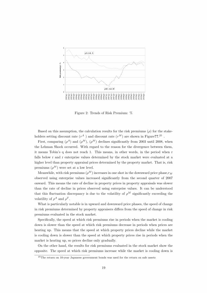
Figure 2: Trends of Risk Premium: %

Based on this assumption, the calculation results for the risk premiums (ρ) for the stake-holders setting discount rate (rA ) and discount rate (rM ) are shown in Figure??.25 .

First, comparing (ρA) and (ρM ), (ρM ) declines significantly from 2003 until 2008, whenthe Lehman Shock occurred. With regard to the reason for the divergence between them,it means Tobin’s q does not reach 1. This means, in other words, in the period when rfalls below r and r enterprise values determined by the stock market were evaluated at ahigher level than property appraisal prices determined by the property market. That is, riskpremiums (ρM ) were set at a low level.

Meanwhile, with risk premiums (ρM ) increases in one shot in the downward price phase,rMobserved using enterprise values increased significantly from the second quarter of 2007onward. This means the rate of decline in property prices in property appraisals was slowerthan the rate of decline in prices observed using enterprise values. It can be understoodthat this fluctuation discrepancy is due to the volatility of ρM significantly exceeding thevolatility of ρA and ρT .

What is particularly notable is in upward and downward price phases, the speed of changein risk premiums determined by property appraisers differs from the speed of change in riskpremiums evaluated in the stock market.

Specifically, the speed at which risk premiums rise in periods when the market is coolingdown is slower than the speed at which risk premiums decrease in periods when prices areheating up. This means that the speed at which property prices decline while the marketis cooling down is slower than the speed at which property prices rise in periods when themarket is heating up, so prices decline only gradually.

On the other hand, the results for risk premiums evaluated in the stock market show theopposite. The speed at which risk premiums increase while the market is cooling down is

25The return on 10-year Japanese government bonds was used for the return on safe assets

19

faster than the speed at which risk premiums decrease while the market is heating up. Inother words, this means that in the stock market, when there are signs of the market coolingdown, values are pushed down at once.

However, when using risk premiums evaluated in the stock market, caution is required.This is because it is known from previous research focusing on the stock market that presentvalues determined from income such as dividends do not necessarily correspond to pricesand risk amounts determined in the stock market, and the volatility of values determined inthe stock market is greater (LeRoy and Porter, 1981; Shiller, 1981).

However, should the change in risk amount that occurred in the stock market therefore bereflected in the property market? It is known that present values determined using dividendincome and prices and risk amounts determined using the stock market are not necessarilymatched (LeRoy and Porter, 1981; Shiller, 1981).26

When, given such previous research, if one reflects ρM determined using the stock marketin the property market, it causes changes in property price to react excessively. On theother hand, with the property appraisal price discount rate, the risk amount (ρA) changesinsufficiently. Based on these results, it can be understood in selecting a discount rate forthe property price index to estimate using the present value model, it is necessary to usethese risk amounts for different purposes or revise them.

4.3 “Investor-Evaluated” Market Value and “Potential” Market

Value

Office Rent Rigidity The property income used in the series of analyses up to this pointwas the actual paying rent. However, since paying rent is often based on leases agreed in thepast, it diverges from the market rent at a specific time, and, what’s more, it is known tohave a high level of viscosity. Therefore, it is possible that “potential” market values usingequivalent rent in the current market (Diewert and Nakamura, 2009) differ significantly fromthe investor-observed REIT enterprise values realized in the REIT market.

Accordingly, we estimated a market rent function based on a hedonic function using actualcontracted rent data.27 We collected 3,985 samples for market rent, and the estimationresults for the hedonic function using these samples is shown in Table4. In estimating thehedonic function, in order to obtain compatibility with other models, we input a locationdummy based on national census survey areas.

Figure3 compares the estimated quality-adjusted office market rent index and the incomeindex for property appraisals estimated in Table4. When both indexes are compared, al-though the overall trends are the same, one can see with respect to the extent of the decreasein rents from 2001 to 2003, the subsequent growth rate of office rents until the third quarter

26When the volatility of discounted cash flow obtained from income and the volatility determined by thestock market are compared, in theory, the volatility determined with discounted cash flow should be greater.However, in reality, it is known that the volatility of prices determined by the stock market is greater (Shiller,1981).

27Market rents were supplied by a major brokerage company. This data is contracted rent that wereactually agreed.

20

Table 4: Estimation Result of Hedonic Equation: Market Office Rent

Coef std err

Constant 9.854 0.091 ***

S : Floor space (m2) 0.000 0.000 ***

A : Age of Building (years) 0.007 0.000 ***

H : Number of stories (stories) 0.013 0.002 ***

TS : Time to the nearest station:(mimutes)

0.018 0.002***

TT : Travel Time to CentralBusiness District (minutes)

0.001 0.001

LD k (k=0,…,K)TD q (q=0,…,Q)

Adjusted Rsquare= 0.556Number of Observations= 3,985

*P<.01, **P<.0.05, ***<.0.01Note: The dependent variable in each case is the log of the price.

Yes

Model.y M

Yes: Census

of 2008, and the extent of the decrease in office rents after the Lehman Shock, in each pe-riod market rents fluctuated by a greater amount than rents used in property appraisals. Inother words, in the office market as well, income indexes used for property appraisals havea high level of viscosity due to the impact of rent under renewed lease and so forth. Thisresult is consistent with research focusing on the housing market (Shimizu, Nishimura, andWatanabe, 2010a).

What is especially notable is the period of market stagnation triggered by the LehmanShock. After peaking in the second quarter of 2008, market rents began to decline, butrents used in appraisals (NOI) reached a peak in the third quarter of 2008. Then, duringthe subsequent decline, rents used in appraisals dropped only slowly, since rents are reducedonly when contracts are renewed.

Estimation of Potential Market Value(Discount Cash Flow) Index Here, we shalltry to estimate an index for prices observed as discounted cash flow using estimated incomeand discount rate. First, with respect to present value PV M,M , we obtained (Y M /rM )with the market rent (Y M ) based on the discount rate rM estimated using enterprise value.With regard to PV A,M , taking the discount rate only as market discount rate rM , we es-timated this using the income Y A used based on property appraisals (yA/rM ). Figure4comparesPV M,M , PV A,M , and the Appraisal price index PV A,A based on property ap-praisal prices.

Taking the first quarter of 2003 as the starting point, each index increases until the so-called mini-bubble of 2007. The average rate of change observed with the geometric average

21

0.8

0.9

1

1.1

1.2

1.3

2001

q220

01q3

2001

q420

02q1

2002

q220

02q3

2002

q420

03q1

2003

q220

03q3

2003

q420

04q1

2004

q220

04q3

2004

q420

05q1

2005

q220

05q3

2005

q420

06q1

2006

q220

06q3

2006

q420

07q1

2007

q220

07q3

2007

q420

08q1

2008

q220

08q3

2008

q420

09q1

2009

q220

09q3

2009

q420

10q1

2010

q220

10q3

2010

q4

YA: Model.yA

YM: Market Rent20

01.2

nd q

uar

ter=

1

Figure 3: Trend of Market Rent and Appraisal Rent Indexes

from the first quarter of 2003 to the first quarter of 2007 was 5.9% for PV M,M , 3.2% forPV A,M , and 2.0% for the appraisal price index PV A,A based on property appraisal prices.This shows PV M,M ’s rate of increase is approximately three times that of PV A,A andPV A,M ’s rate of increase is approximately 1.5 times that of PV A,A.

Focusing here on the time of peaking out, compared to PV M,M and PV M,A(first quarterof 2007), there was a lag of 1.5 years in the movement of PV A,A(third quarter of 2008).

In other words, when rent is converted from paying rent to market rent, even though thereis an impact on the magnitude of price fluctuations, there is no change in the time of peakingout. Meanwhile, in the case of risk premiums obtained from market-derived discount rates,it is found that there is a possibility of identifying the market tipping point at an earlierstage.

5 Conclusion: Issues in conducting of Commercial Prop-

erty Price Indexes

With regard to the estimation of commercial property price indexes, appraisal-based prop-erty price indexes have been published for many years focusing on Japan, the U.S., and theU.K. With these indexes being used, questions have been raised about whether fluctuationsin appraisal-based property price indexes diverge from actual market conditions, and con-siderable research has been conducted in order to clarify the distortion in appraisal-basedproperty price as well as revising them. Furthermore, in recent years, commercial propertytransaction price indexes have been developed and started to be published in the U.S.

However, in many countries, such as Japan, since not enough transaction price data is

22

0.8

1

1.2

1.4

1.6

1.8

2

2.2

2.4

2.6

2003

q120

03q2

2003

q320

03q4

2004

q120

04q2

2004

q320

04q4

2005

q120

05q2

2005

q320

05q4

2006

q120

06q2

2006

q320

06q4

2007

q120

07q2

2007

q320

07q4

2008

q120

08q2

2008

q320

08q4

2009

q120

09q2

2009

q320

09q4

2010

q120

10q2

2010

q320

10q4

PV(M,M): YM / rM

PV(M,A): YM / rA2

VM3(Hybrid): Model.VM2

2003

.1nd

qu

arte

r=1

Figure 4: Trend of Present Value Indexes

provided/collected, many difficulties accompany the estimation of indexes based on transac-tion prices. In addition, compared to housing and so forth, commercial property has a highlevel of heterogeneity, so quality adjustment must be rigorously performed.

In addressing problems such as this lack of data and rigorous quality adjustment, one mayrefer to past experience and efforts that have been made in the practical property appraisal.Residential property appraisal prices are determined based on the sales comparison approach,using comparables for similar transactions in the vicinity of the property being appraised.For housing price indexes, this leads to the price index being estimated by performing qualityadjustment through direct use of transaction prices.

For commercial property, on the other hand, since there is lack of transaction comparablesas well as a high level of heterogeneity, it has been recognized it is difficult to perform ap-praisal based on the sales comparison approach. As a result, commercial property appraisalsare generally determined with present value, based on a method known as the capitalizationmethod. This means that the difficulty level of estimating commercial property price indexesusing transaction prices is extremely high compared to housing.

In this study, based on past experience in the practical property appraisal, we explored thepossibility of estimating a price index based on a present value model. Specifically, focusingon the Tokyo area, we estimated a present value-based property price index, using publishedJ-REIT data with the same characteristics as data possessed by NCREIF in the U.S., IPDin the U.K., etc. The following provides an overview of the analysis and results obtained.

In estimating present value, the determination of discount rate is extremely important.Income, which is the numerator, is already finalized by the market, so it is difficult to imaginethat significant differences would occur between property appraisers and transactors whenforecasting it. However, it is to be expected there would be significant differences between

23

the respective stakeholders with respect to the risk premiums for property forming thediscount rate. Accordingly, we obtained the discount rate for property appraisal prices andtransaction prices and the discount rate using enterprise values able to be obtained usingthe J-REIT investment unit market, and estimated the respective risk premiums.

Accordingly, along with the discount rate for property appraisal prices and transactionprices, we obtained the discount rate using enterprises values able to obtained in the J-REITinvestment unit market, and estimated the respective risk premiums.

The results showed there was significant divergence between the risk premiums set withproperty appraisals (ρA) and with transactions (ρT )and the risk premium for property in-vestments formed by the stock market (ρM )– in particular, ρM was significantly lower from2003 until 2008, when the Lehman Shock occurred. With regard to the reason for the diver-gence between them, it is significant that Tobin’s q does not reach 1, which means enterprisevalues determined by the stock market were evaluated at a higher level than property ap-praisal prices and transaction prices determined by the property market. In other words,risk premiums (ρM ) determined through the stock market were set at a low level. Thatis, it was understood the difference between these discount rates and the prices determinedthrough them is caused by differences in the risk premiums.

Moreover, if one looks at the extent of risk premium fluctuation, the volatility of riskpremiums formed in the stock market (ρM ) is greater than those of (ρA) or (ρT ) hypothesizedwith appraisals or transactions. In other words, as indicated by Shillers’ Test (Shiller, 1981)and clarified by many subsequent studies focusing on the stock market, risk premiums (ρM )formed in the stock market fluctuate more than risk premiums (ρA) or (ρT ) determined withpresent values. On the other hand, as indicated by the term smoothing problem, since thefluctuation of risk premiums set with appraisals (ρA) is extremely gradual, it is said theydo not accurately represent market conditions either. In such a case, in determining presentvalue, it is important to consider changes in the market while also referring to risk premiumsformed in the stock market (ρM ).

In terms of issues that should be kept in mind when estimating property price indexesusing property appraisal values and using them in policy, these results led to the followingconclusions.

Focusing on trends for risk premiums determined by property appraisers and risk pre-miums formed in the stock market, which were estimated as described above, the resultspredicted that risk premiums determined by property appraisers may not be able to beevaluated properly in periods when the market is cooling down or stagnating. Specifically,the speed at which risk premiums are increased in periods when the market is stagnatingis relatively gradual compared to the speed at which risk premiums are decreased whenprices are heating up. Meanwhile, risk premiums observed in the stock market showed theopposite results. Based on these estimation results, it is possible risk premiums determinedby property appraisers are not set properly in periods of the market cooling down, and as aresult of this, even after the Lehman Shock, property price indexes declined only gradually.

In terms of the reason for this, as Crosby, Lizieri, and McAllister (2009) have made

24

clear, one possibility is that pressure is exists from the property appraisal client. The partyordering a property appraisal report is a J-REIT investment company. During periods whenthe market is heating up, investment companies that manage J-REITs have an incentive toincrease property prices appropriately in accordance with changes in the market. On theother hand, when the market is stagnating, there is an incentive to maintain the investmentcompany’s LTV within a certain ratio, which raises the question of whether these companiesmay have urged property appraisers not to lower property appraisal prices. This issue shouldbe addressed going forward when estimating property price indexes using property appraisalinformation.

As well, the income (yA) determined in the property investment market is paying rent.With regard to paying rent, when it is paid based on rent agreed in leases concluded inthe past, there are times when it diverges significantly from the market conditions. Inparticular, in periods when market rents increase or decrease significantly, the divergence isconsiderable. Accordingly, we estimated a market rent index using actual contracted rents.Using the market rent index estimated in this manner and the discount rates obtainedpreviously, we estimated multiple present value indexes. Specifically, we estimated two newprice indexes that obtained the present value PVM,M (obtained with the discount rate rM

estimated using market rent yM and enterprise value) and the present value PVM,A (usingthe discount rate rA used based on property appraisals and market rent yM taking thelatter as income only). Comparing the two estimated indexes and transaction price indexVM3 based on property appraisal prices showed that compared to PVM,M , which peakedout in the first quarter of 2007, PVM,A moved with a lag of one year (peaking out in the firstquarter of 2008) and VM3 moved with a lag of 1.5 years (peaking out in the third quarterof 2008).

This raises the issue of how to establish the definition and nature of property pricesdetermined as present values in the policy field. In other words, there is a possibility thatprice stickiness or rigidity of price is inherent in property prices determined using revenuebased on current paying rent as a basis, and what’s more, the primary value level also variessignificantly.

The estimation of commercial property price indexes is restricted in different ways basedon the data that is available in different countries. In countries where data for the propertyinvestment market is available, it is possible to use both property appraisal price dataand transaction price data. For such countries, it is perhaps necessary to outline howproperty appraisal prices should be modified after understanding their mechanism. Aswell, in countries where the investment market is undeveloped, indexes are estimated aftercollecting/preparing transaction prices. In such countries, since it is difficult to obtainproperty characteristics data, there are many problems accompanying the application of thehedonic method.

With the strong data limitations in different countries, when it comes to the preparationof commercial property price indexes, one must perhaps select the estimation method basedon the available data and consider how to prepare it.

25

References

[1] Bokhari,S and D. Geltner (2010),“Estimating Real Estate Price Movements for HighFrequency Tradable Indexes in a Scarce Data Environment,” Juornal of Real EstateFinance and Economics, (forthcoming; published online 22.July.2010)

[2] Clayton, J., D. Geltner. and S.W.Hamilton (2001),“Smoothing in Commercial PropertyValuations: Evidence from Individual Appraisals,” Real Estate Economics, 29, pp.337-360.

[3] Crosby, N., Devaney, S., T.Key and G.Matysiak. (2003), “Valuation Accuracy: Recon-ciling the Timing of the Valuation and Sale, Working Papers in Real Estate & Planning06/03, University of Reading.

[4] Crosby, N., C.Lizieri and P.McAllister (2009),“Means, Motive and Opportunity? Dis-entangling Client Influence on Performance Measurement Appraisals, Working Papersin Real Estate & Planning 09/09, University of Reading.

[5] Devaney,S and R. M. Diaz (2009),“Transaction based indices for the UK commercialproperty market: exploration and evaluation using IPD data,” University of AberdeenBusiness school,Discussion Paper 2010-02.

[6] Diewert, W.E. (2007), “The Paris OECD-IMF Workshop on Real Estate Price In-dexes:Conclusions and Future Directions”, Discussion Paper 07-01, Department of Eco-nomics, University of British Columbia, Vancouver, British Columbia,Canada, V6T1Z1.

[7] Diewert, W.E.and A.Nakamura (2009), “Accounting for Housing in a CPI,” DiscussionPaper 09-08, Department of Economics, University of British Columbia, Vancouver,British Columbia,Canada, V6T 1Z1.

[8] Diewert, W.E.and C.Shimizu (2012), “House Price Indexes andthe Global Financial Crisis,” available at: http://www.cs.reitaku-u.ac.jp/sm/shimizu/Essay/A/111215DiewertShimizu.pdf (Nikkei Janualy 13, 2012.inJapanese).

[9] Diewert, W.E.J. de Haan and R. Hendriks (2010), “The Decomposition of a House Priceindex into Land and Structures Components:A Hedonic Regression Approach”, Discus-sion Paper 10-01, Department of Economics, University of British Columbia,Vancouver,British Columbia,Canada, V6T 1Z1.

[10] Ekeland, I., J. J. Heckman and L. Nesheim, (2004), “Identification and Estimation ofHedonic Models,” Journal of Political Economy, Vol.112, pp.60-109

[11] Hayashi, F., and T. Inoue (1991), “The relation between firm growth and Q with mul-tiple capital goods: Theory and evidence from panel data on Japanese firms,” Econo-metrica, pp.731–753.

26

[12] Fisher.J, D. Geltner, and R.B.Webb (1994),“Value Indices of Commercial Real Es-tate:A Comparison of Index Construction Methods,” Juornal of Real Estate Financeand Economics, 9, pp.137–164.

[13] Fisher, J., D. Gatzlaff, D. Geltner and D.Haurin (2003),“Controlling for the Impact ofVariable Liquidity in Commercial Real Estate Price Indices,” Real Estate Economics,31, pp.269-303.

[14] Fisher.J, D.Geltner, and H.Pollakowski (2007),“A Quarterly Transactions-Based Index(TBI) of Institutional Real Estate Investment Performance and Movements in Supplyand Demand,” Journal of Real Estate Finance and Economics, 34, pp.5–33.

[15] Geltner,D (1997),“The use of appraisals in portfolio valuation and index,”Journal ofReal Estate Finance and Economics, 15,pp.423–445.

[16] Geltner, D. and W. Goetzmann (2000),“Two Decades of Commercial Property Returns:A Repeated-Measures Regression-Based Version of the NCREIF Index,” Journal of RealEstate Finance and Economics, 21,pp.5-21.

[17] Geltner,D R.A. Graff and M.S.Young (1994),“Random Disaggregate Appraisal Error inCommercial Property, Evidence from the Russell-NCREIF Database,”Journal of RealEstate Research,9(4),pp403-419.

[18] Geltner,D and H. Pollakowski (2007),“A Set of Indexes for Trading Commercial RealEstate Based on the Real Capital Analytics Transaction Prices Database,”available at:http://mit.edu/cre/research/credl/rca/MIT-wp-r2.pdf

[19] Gordon, M.J (1959), “Dividends, Earnings, and Stock Prices,” The Review of Eco-nomics and Statistics, Vol. 41, pp. 99-105.

[20] Jorgenson, D. W (1963),“Capital Theory and Investment Behavior,” American Eco-nomic Review, 53, pp.247-259.

[21] LeRoy,S.F and R. D. Porter (1981),“The Present-Value Relation: Tests Based on Im-plied Variance Bounds,” Econometrica, Vol. 49, No. 3, pp.555-574.

[22] Nishimura,K.G and C.Shimizu (2003) , “Distortion in Land Price Information-Mechanism in Sales Comparables and Appraisal Value Relation-,” Center of Inter-national Research on the Japanese Economy Discussion Paper(University of Tokyo),No.195, available at:http://www.cs.reitaku-u.ac.jp/sm/shimizu/Paper/2003cf195.pdf

[23] Quan, D.C and J.M.Quigley (1991), “Price Formation and the Appraisal Function inReal Estate Markets,” Journal of Real Estate Finance and Economics, 4,pp127-146.

[24] Shiller,R. J (1981),“Do Stock Prices Move Too Much to be Justified by SubsequentChanges in Dividends?,” American Economic Review, Vol. 71, No. 3, pp. 421-436.

27

[25] Shimizu,C and K.G.Nishimura (2006), “Biases in appraisal land price information: thecase of Japan,” Journal of Property Investment and Finance, 24, No.2，pp. 150- 175.

[26] Shimizu,C and K.G.Nishimura (2007), “Pricing structure in Tokyo metropolitan landmarkets and its structural changes: pre-bubble, bubble, and post-bubble periods,”Journal of Real Estate Finance and Economics, 35(4),pp.495-496.

[27] Shimizu,C, K.G.Nishimura and T.Watanabe (2010a), “Residential Rents and PriceRigidity: Micro Structure and Macro Consequences,”Journal of Japanese and Inter-national Economy,Vol.24, pp282-299.

[28] Shimizu,C, K.G.Nishimura and T.Watanabe (2010b), “House Prices in Tokyo - A Com-parison of Repeat-sales and Hedonic measures-,” Journal of Economics and Statistics,Vol.230(6), pp.792-813.

[29] Shimizu,C, K.G.Nishimura and T.Watanabe (2011), “House Prices at Dif-ferent Stages of the Buying/Selling Process,” Research Center for PriceDynamics Working Paper Series No.69..available at: http://www.cs.reitaku-u.ac.jp/sm/shimizu/Paper/IFD WP69.pdf

[30] Shimizu,C, K.G.Nishimura and T.Watanabe (2012), “House prices from magazines,realtors, and the Land Registry,” BIS Papers, No 64(Property markets and financialstability) ,29-38.

[31] Shimizu,C, K.G.Nishimura and T.Watanabe (2012), “Biases in commercial appraisal-based property price indexes － Lessons from Japanese experience in Bubble period－,”CARF Working Paper(Mimeo), Center for Advanced Research in Finance of theUniversity of Tokyo.

[32] Tobin, J. (1969),“A general equilibrium approach to monetary theory,” Journal ofMoney Credit and Banking 1 (1), pp.15-29.

28

Present Value and the Commercial Property Price

Documents

Transcript of Present Value and the Commercial Property Price