Preparation for Calculus

P

Graphs and ModelsP.1

3

The Graph of an Equation

4

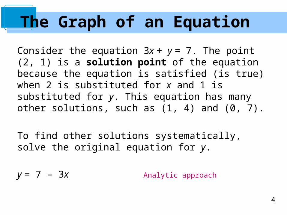
Consider the equation 3x + y = 7. The point (2, 1) is a solution point of the equation because the equation is satisfied (is true) when 2 is substituted for x and 1 is substituted for y. This equation has many other solutions, such as (1, 4) and (0, 7).

To find other solutions systematically, solve the original equation for y.

y = 7 – 3x Analytic approach

The Graph of an Equation

5

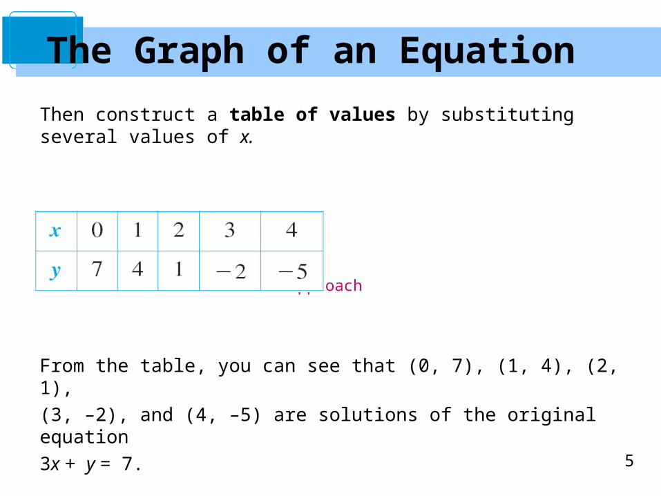
Then construct a table of values by substituting several values of x.

Numerical approach

From the table, you can see that (0, 7), (1, 4), (2, 1),

(3, –2), and (4, –5) are solutions of the original equation

3x + y = 7.

The Graph of an Equation

6

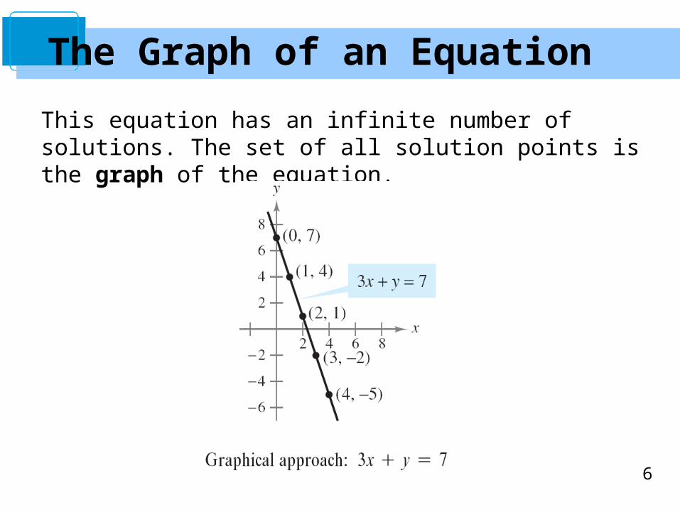
This equation has an infinite number of solutions. The set of all solution points is the graph of the equation.

The Graph of an Equation

7

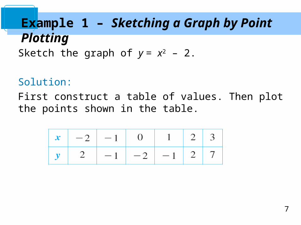
Sketch the graph of y = x2 – 2.

Solution:

First construct a table of values. Then plot the points shown in the table.

Example 1 – Sketching a Graph by Point Plotting

8

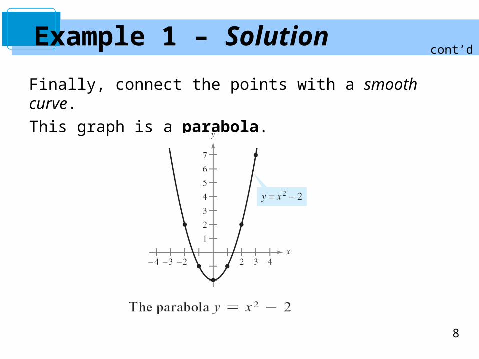
Finally, connect the points with a smooth curve.

This graph is a parabola.

Example 1 – Solutioncont’d

9

Intercepts of a Graph

10

Intercepts of a Graph

Two types of solution points that are especially useful in graphing an equation are those having zero as their x- or y-coordinate.

Such points are called intercepts because they are the points at which the graph intersects the x- or y-axis.

The point (a, 0) is an x-intercept of the graph of an equation if it is a solution point of the equation.

11

Intercepts of a Graph

To find the x-intercepts of a graph, let y be zero and solve the equation for x.

The point (0, b) is a y-intercept of the graph of an equation if it is a solution point of the equation.

To find the y-intercepts of a graph, let x be zero and solve the equation for y.

12

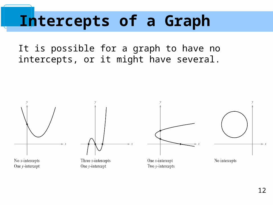
It is possible for a graph to have no intercepts, or it might have several.

Intercepts of a Graph

13

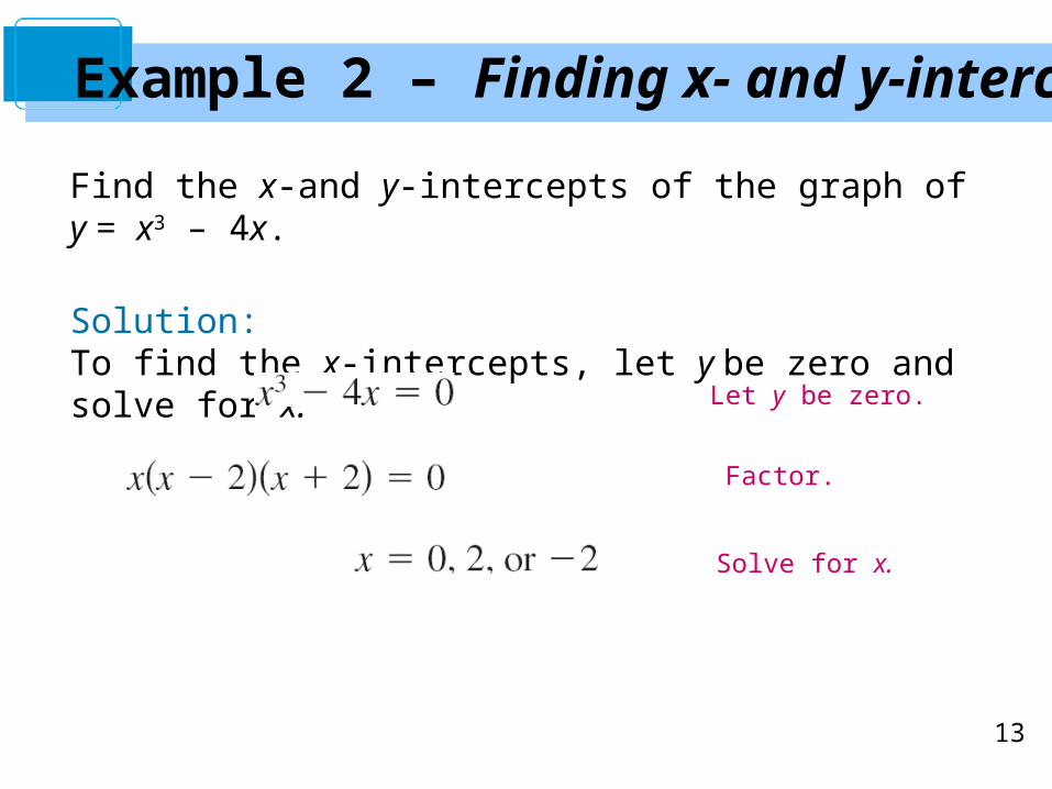
Example 2 – Finding x- and y-intercepts

Find the x-and y-intercepts of the graph of y = x3 – 4x.

Solution:To find the x-intercepts, let y be zero and solve for x.

Let y be zero.

Factor.

Solve for x.

14

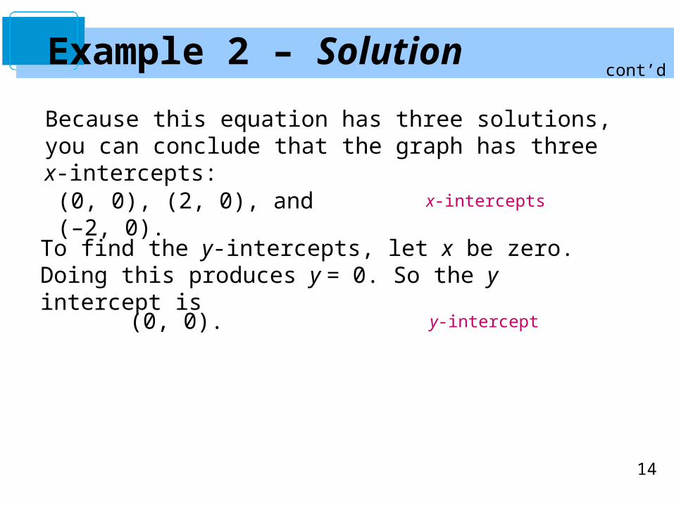
Example 2 – Solution

Because this equation has three solutions, you can conclude that the graph has three x-intercepts:

(0, 0), (2, 0), and (–2, 0).

y-intercept

To find the y-intercepts, let x be zero. Doing this produces y = 0. So the y intercept is

(0, 0).

x-intercepts

cont’d

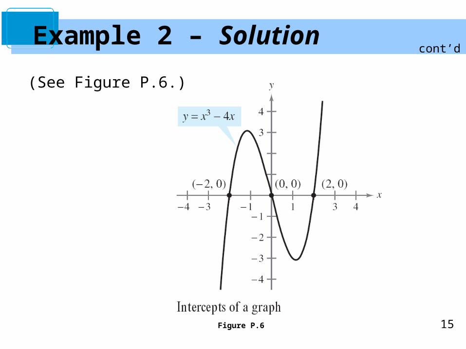
15Figure P.6

Example 2 – Solution

(See Figure P.6.)

cont’d

16

Symmetry of a Graph

17

Symmetry of a Graph

Knowing the symmetry of a graph before attempting to sketch it is useful because you need only half as many points to sketch the graph.

The following three types of symmetry can be used to help sketch the graphs of equations.

18

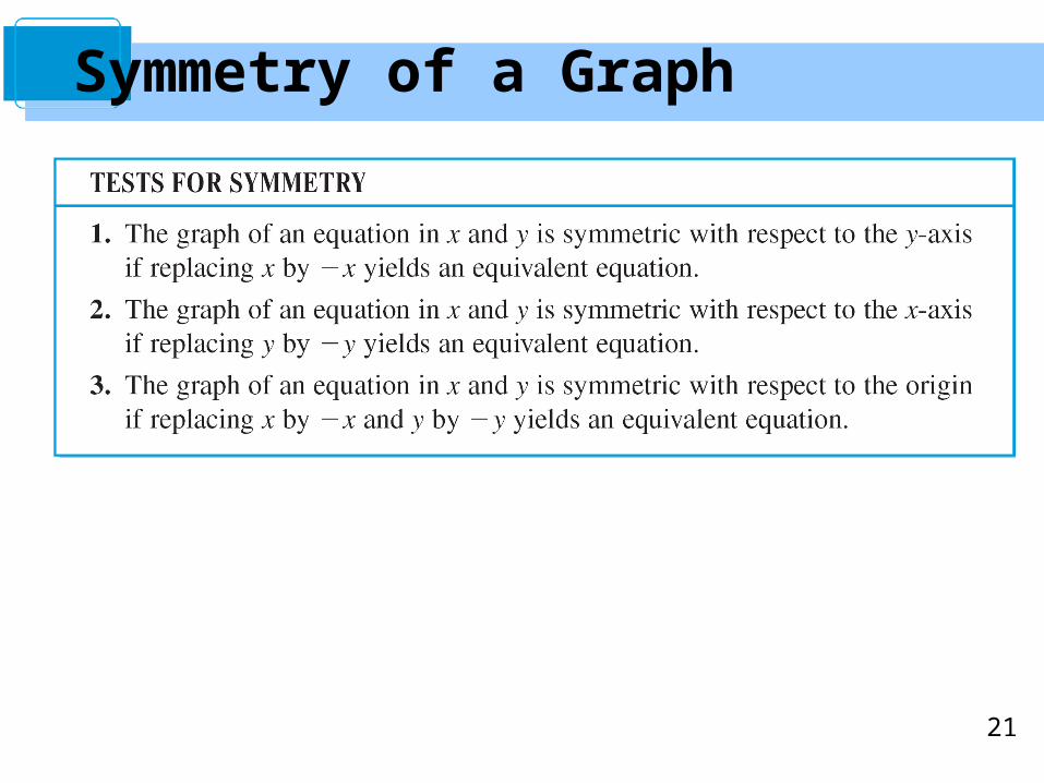
1. A graph is symmetric with respect to the y-axis if, whenever (x, y) is a point on the graph, (–x, y) is also a point on the graph. This means that the portion of the graph to the left of the y-axis is a mirror image of the portion to the right of the y-axis.

Symmetry of a Graph

19

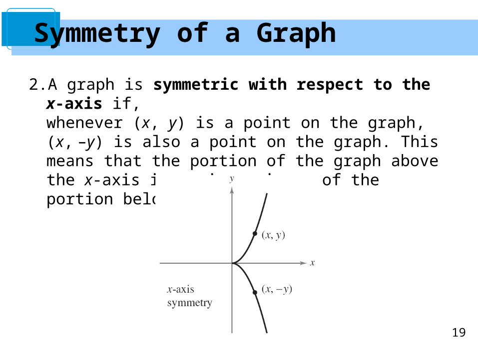
2. A graph is symmetric with respect to the x-axis if, whenever (x, y) is a point on the graph, (x, –y) is also a point on the graph. This means that the portion of the graph above the x-axis is a mirror image of the portion below the x-axis.

Symmetry of a Graph

20

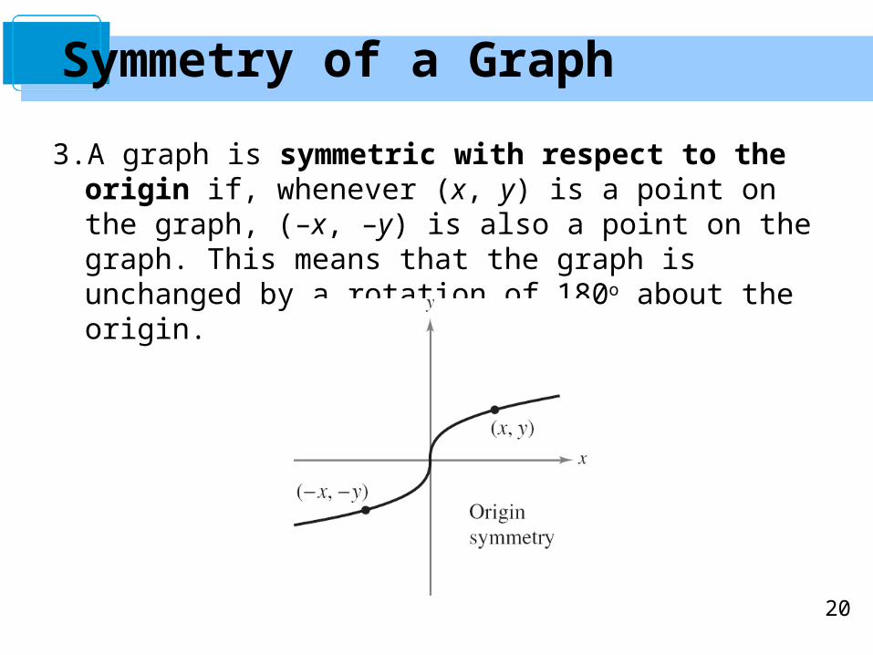
3. A graph is symmetric with respect to the origin if, whenever (x, y) is a point on the graph, (–x, –y) is also a point on the graph. This means that the graph is unchanged by a rotation of 180o about the origin.

Symmetry of a Graph

21

Symmetry of a Graph

22

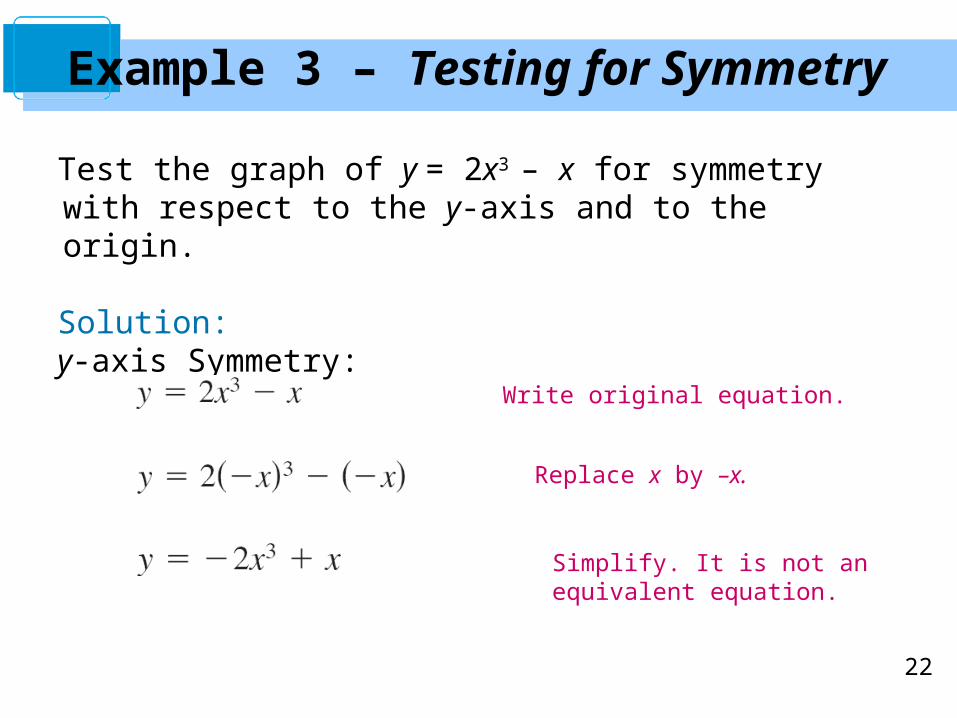
Example 3 – Testing for Symmetry

Test the graph of y = 2x3 – x for symmetry with respect to the y-axis and to the origin.

Solution:y-axis Symmetry:

Write original equation.

Replace x by –x.

Simplify. It is not an equivalent equation.

23

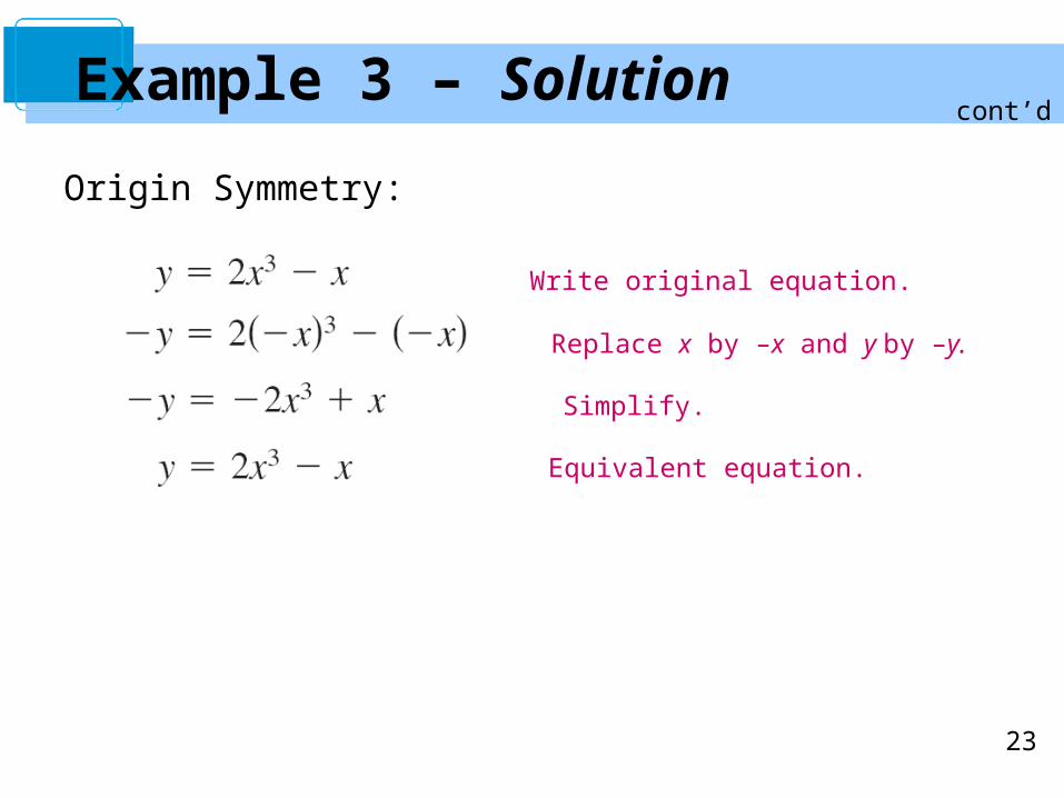
Example 3 – Solution

Origin Symmetry:

Write original equation.

Replace x by –x and y by –y.

Simplify.

Equivalent equation.

cont’d

24

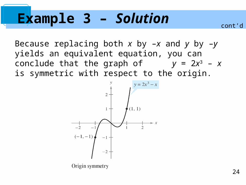
Because replacing both x by –x and y by –y yields an equivalent equation, you can conclude that the graph of y = 2x3 – x is symmetric with respect to the origin.

Example 3 – Solutioncont’d

25

Points of Intersection

26

A point of intersection of the graphs of two equations is a point that satisfies both equations.

You can find the point(s) of intersection of two graphs by solving their equations simultaneously.

Points of Intersection

27

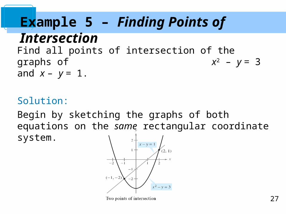
Find all points of intersection of the graphs of x2 – y = 3 and x – y = 1.

Solution:

Begin by sketching the graphs of both equations on the same rectangular coordinate system.

Example 5 – Finding Points of Intersection

28

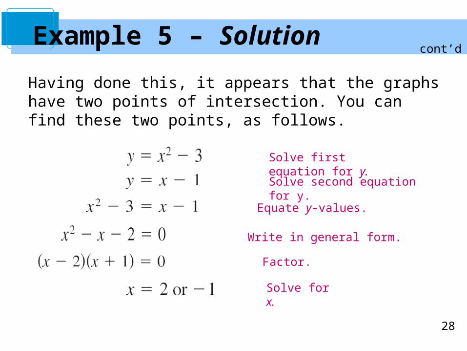
Having done this, it appears that the graphs have two points of intersection. You can find these two points, as follows.

Example 5 – Solution

Solve first equation for y.

Solve second equation for y.

Equate y-values.

Write in general form.

Factor.

Solve for x.

cont’d

29

The corresponding values y of are obtained by substitutingx = 2 and x = –1 into either of the original equations.

Doing this produces two points of intersection:

(2, 1) and (–1, –2). Points of intersection

Example 5 – Solutioncont’d

30

Mathematical Models

31

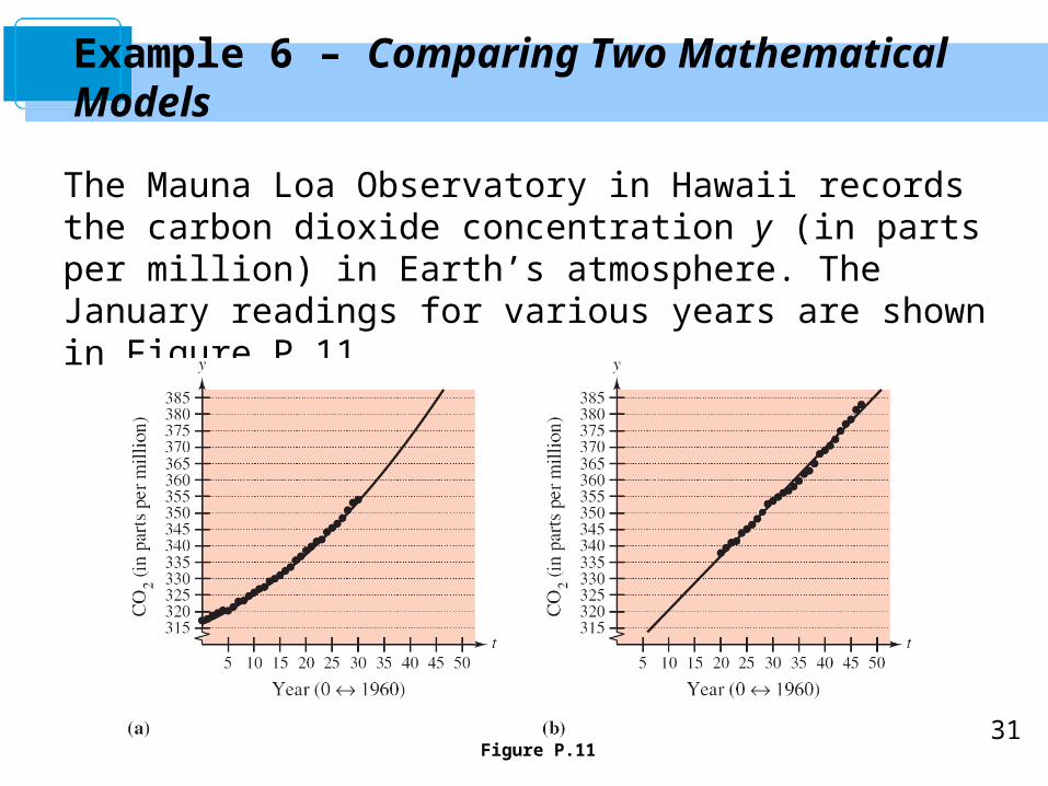
Example 6 – Comparing Two Mathematical Models

The Mauna Loa Observatory in Hawaii records the carbon dioxide concentration y (in parts per million) in Earth’s atmosphere. The January readings for various years are shown in Figure P.11.

Figure P.11

32

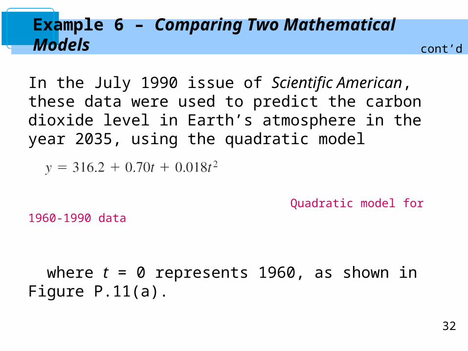
In the July 1990 issue of Scientific American, these data were used to predict the carbon dioxide level in Earth’s atmosphere in the year 2035, using the quadratic model

Quadratic model for 1960-1990 data

where t = 0 represents 1960, as shown in Figure P.11(a).

Example 6 – Comparing Two Mathematical Models cont’d

33

The data shown in Figure P.11(b) represent the years 1980 through 2007 and can be modeled by

Linear model for 1980–2007 data

where t = 0 represents 1960.

What was the prediction given in the Scientific American article in 1990? Given the new data for 1990 through 2007, does this prediction for the year 2035 seem accurate?

Example 6 – Comparing Two Mathematical Models cont’d

34

Example 6 – Solution

To answer the first question, substitute t = 75 (for 2035) into the quadratic model.

Quadratic model

So, the prediction in the Scientific American article was that the carbon dioxide concentration in Earth’s atmosphere would reach about 470 parts per million in the year 2035.

35

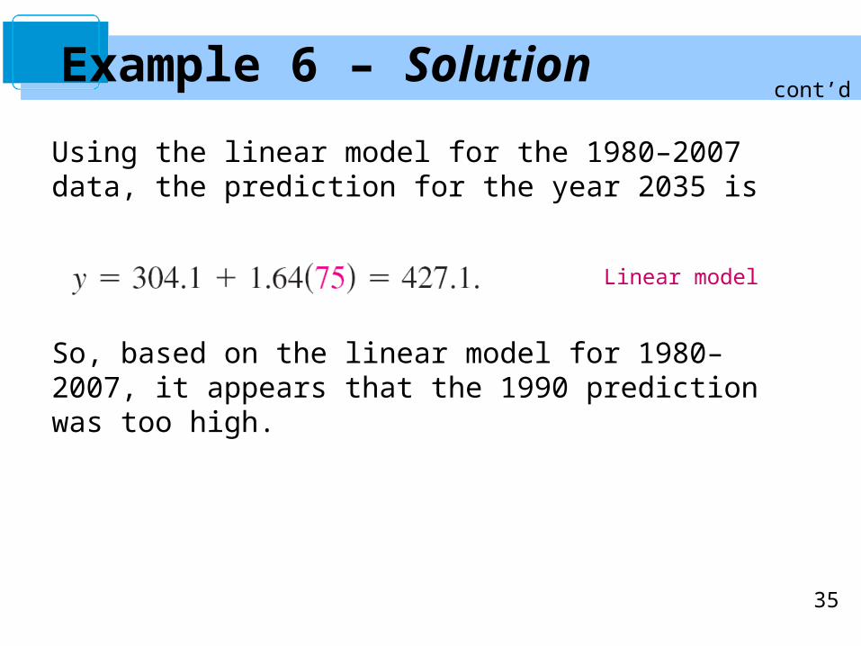
Using the linear model for the 1980–2007 data, the prediction for the year 2035 is

So, based on the linear model for 1980–2007, it appears that the 1990 prediction was too high.

cont’d

Linear model

Example 6 – Solution