Preliminarydraft* SELF2FULFILLINGCRISESINTHEEUROZONE ... · % 2% 1. Introduction* The financial%...

Preliminary draft

SELF-‐FULFILLING CRISES IN THE EUROZONE. AN EMPIRICAL TEST

Paul De Grauwe

London School of Economics and CEPS

Yuemei Ji LICOS, University of Leuven

Abstract: We test the hypothesis that the government bond markets in the Eurozone are more fragile and more susceptible to self-‐fulfilling liquidity crises than in stand-‐alone countries. We find evidence that a significant part of the surge in the spreads of the PIGS countries in the Eurozone during 2010-‐11 was disconnected from underlying increases in the debt to GDP ratios, and was the result of negative self-‐fulfilling market sentiments that became very strong since the end of 2010. We argue that this can drive member countries of the Eurozone into bad equilibria. We also find evidence that after years of neglecting high government debt, investors became increasingly worried about this in the Eurozone, and reacted by raising the spreads. No such worries developed in stand-‐alone countries despite the fact that debt to GDP ratios were equally high and increasing in these countries.

April 2012 Paper prepared for the Danmarks Nationalbank/JIMF Conference on the Sovereign Debt Crisis, Copenhagen, April 13-‐14, 2012.We are grateful to Geert Dhaene and Daniel Gros for insightful comments.

2

1. Introduction

The financial crisis that erupted in the industrialized world in 2007 forced

governments to save their domestic banking systems from collapse and to

sustain their economies that experienced their sharpest postwar recession. As a

result, these governments saw their debt levels increase dramatically. Figure 1

shows this for the US, the UK and the Eurozone.

Figure 1 is also interesting for another reason. We observe that the increase in

the debt to GDP ratios since 2007 is significantly faster in the US and the UK than

in the Eurozone, so much so that at the end of 2011 the US surpassed the

Eurozone’s debt to GDP ratio and the UK is soon to do so. Yet it is the Eurozone

that has experienced a severe sovereign debt crisis and not the US nor the UK.

The severity of the sovereign debt crisis in the Eurozone is illustrated in Figure 2,

which shows the spectacular increase in the spreads of a large number of

Eurozone countries1.

In De Grauwe(2011) a theory of the fragility of the Eurozone is developed that

explains why the Eurozone countries are more prone to experience a sovereign

debt crisis than countries that are not part of a monetary union even when these

countries experience a worse fiscal situation. The purpose of this paper is to

provide a further empirical test of this theory.

Section 1 summarizes the main features of the fragility theory of the Eurozone

and derives the testable implications. Section 2 presents some preliminary data

and section 3 describes the econometric testing procedure and discusses the

results. Section 4 derives some policy implications.

1 The spreads are defined as the differences of 10-‐year government bond rates of each country with teh German government bond rate.

3

Figure 1

Source: European Commission, Ameco Figure 2

Source: Datastream

4

2. The fragility of the Eurozone

The key to understanding the sovereign debt crisis in the Eurozone has to do

with an essential feature of a monetary union2. Members of monetary union

issue debt in a currency over which they have no control. As a result the

governments of these countries cannot give a guarantee that the cash will always

be available to pay out bondholders at maturity. It is literally possible that these

governments find out that the liquidity is lacking to pay out bondholders.

This is not the case in “stand-‐alone countries”, i.e. countries that issue debt in

their own currency. These countries can give a guarantee to the bondholders

that the cash will always be available to pay them out. The reason is that if the

government were to experience a shortage of liquidity it would call upon the

central bank to provide the liquidity. And there is no limit to the capacity of a

central bank to do so.

The absence of a guarantee that the cash will always be available creates a

fragility in a monetary union. Member countries are susceptible to movements of

distrust. When investors fear some payment difficulty, e.g. triggered by a

recession, they sell the government bonds. This has two effects. It raises the

interest rate and leads to a liquidity outflow as the investors who have sold the

government bonds look for safer places to invest. This “sudden stop” can lead to

a situation in which the government cannot roll over its deb except at prohibitive

interest rates.

The ensuing liquidity crisis can easily degenerate into a solvency crisis. As the

interest rate shoots up, the country is likely to be pushed into a recession. This

tends to reduce government revenues and to increase the deficit and debt levels.

The combination of increasing interest rates and debt levels can push the

government into default.

There is a self-‐fulfilling element in this dynamics. When investors fear default,

they act in such a way that default becomes more likely. A country can become

insolvent because investors fear default.

2 See De Grauwe(2011) for a more detailed analysis. See also (see Kopf(2011))

5

The problem of member countries of a monetary union described in the previous

paragraphs is similar to the problems faced by emerging countries that issue

debt in a foreign currency, usually the dollar. These countries can be confronted

with a “sudden stop” when capital inflows suddenly stop leading to a liquidity

crisis (see Calvo, et al. (2006)). This problem has been analyzed intensively by

economists, who have concluded that financial markets acquire great power in

these countries and can force them into default (see Eichengreen, et al. ()).

The liquidity crises in a monetary union also make it possible for the emergence

of multiple equilibria. Countries that are distrusted by the market are forced into

a bad equilibrium characterized by high interest rates, the need to impose strong

budgetary austerity programs that push these countries into a deep recession.

Conversely, countries that are trusted become the recipients of liquidity inflows

that lower the interest rate and boost the economy. They are pushed into a good

equilibrium. In De Grauwe(2011) a formal model inspired by the

Obsetfeld(1986) model of foreign currency crises is presented in which multiple

equilibria are a possible outcome3. In appendix a simple version of this model is

presented.

Finally it should also be mentioned that the fragility of member countries of a

monetary union has a similar structure as the fragility of banks. The latter are

fragile because the unbalanced maturity structure of their assets and liabilities.

The latter have shorter maturities than the former (“banks borrow short and

lend long”). As a result, banks are vulnerable to runs; When depositors fear

liquidity problems they run to the bank to convert their deposits into cash

thereby precipitating the liquidity crisis that they are fearing. (See the classic

model of bank runs of Diamond and Dybvig(1983)). This problem can be solved

by the central bank promising to step in and to provide liquidity in times of crisis

(“lender of last resort”).

Governments in a monetary union that cannot rely on a lender of last resort face

a similar fragility. Their liabilities (bonds) are liquid and can be converted into 3 There exist many formal theoretical models that create self-‐fulfilling liquidity crises. Many of these have been developed for explaining crises in the foreign exchange markets (see Obstfeld(1986)). Other models have been applied to the government debt (Calvo(1988), Gros(2011), Corsetti and Dedola(2011)).

6

cash quickly. The government assets, (physical assets, claims on taxpayers),

however, are illiquid. In the absence of a central bank that is willing to provide

liquidity, these governments can be pushed into a liquidity crisis because they

cannot transform their assets into liquid funds quickly enough.

3. How to test the theory?

The theory presented in the previous section leads to a number of testable

propositions.

We have seen that in a monetary union movements of distrust vis-‐à-‐vis one

country leads to an increase in the government bond rate of that country and

thus to an increase in the spread (the difference) with the bond rates of other

countries. When such movements of distrust occur these spreads are likely to

increase significantly without much movement of the underlying fundamentals

that influence the solvency of the country. Movements in the spreads will then be

typically much higher than the movements in the underlying fundamentals It

will then appear that the spreads are dissociated from these fundamentals4.

Thus one way to test the theory is first to estimate a model of the spreads, which

relates the latter to the fundamental variables of the spreads. In a second stage

we will want to track the deviations of the observed spreads from the spreads as

estimated by the model. More specifically we wish to identify periods during

which market sentiments drive the spreads away from their underlying

fundamentals.

In order for such a test to be convincing it will be important to analyze a control

group of countries that do not belong to a monetary union. We will therefore

take a sample of “stand-‐alone” countries and analyze whether in this control

group one observes similar movements of the spreads away from their

underlying fundamentals. Our theory predicts that this should not happen in

countries that have full control over the currency in which they issue their debt.

4 Note that we are not implying that fundamentals do not matter; in fact small movements of fundamentals can trigger large movements in spreads, because they trigger the fear factor (like in a bank run).

7

4. The facts about spreads and debt to GDP ratios

Before performing a rigorous econometric analysis explaining the spreads, it is

useful to look at how the spreads and the debt to GDP ratios have evolved over

time in the Eurozone and in the sample of “stand-‐alone” countries. We look at

the relation between the spreads and the debt to GDP ratio, as the latter is the

most important fundamental variable influencing the spreads (as will become

clear from our econometric analysis).

We first present the relation between the spreads and the debt-‐to-‐GDP ratios in

the Eurozone. This is done in Figure 3, which shows the spreads on vertical axis

and the debt to GDP ratios on the horizontal axis in the Eurozone countries. Each

point is a particular observation of one of the countries in a particular quarter

(sample period 2000Q1-‐2011Q3). We also draw a straight line obtained from a

simple regression of the spread as a function of the debt to GDP ratio.

We observe first that there is a positive relation (represented by the positively

sloped regression line) between the spread and the debt to GDP ratio, i.e. higher

spreads are associated with higher debt to GDP ratios. We will return to this

relationship and present more precise statistical results in the next section.

A second observation to be made from Figure 3 is that the deviations from the

fundamental line (the regression line) appear to occur in bursts that are time

dependent. We show this in Figure 3, which is the same as Figure 2 but where we

have highlighted all observations that are more than 3 standard deviations from

the fundamental line in a triangle. It is striking to find that all these observations

concern three countries (Greece, Portugal and Ireland) and that these

observations are highly time dependent, i.e. the deviations start at one particular

moment of time and then continue to increase in the next consecutive periods.

Thus, the dramatic increases in the spreads that we observe in these countries

from 2010 on do not appear to be much related to the increase in the debt to

GDP ratios during the same period. This is as the theory predicts. We will analyze

whether this results stands the scrutiny of econometric testing.

8

Figure 3: Spreads and debt to GDP ratio in Eurozone (2000Q1-‐2011Q3)

Source: Eurostat and datastream..

Figure 4: Spreads and debt to GDP ratio in Eurozone (2000Q1-‐2011Q3)

Source: Eurostat and datastream.

-‐2

0

2

4

6

8

10

12

14

16

0 20 40 60 80 100 120 140 160

Debt to GDP ratio (%)

Government bond spread (%

)

GR2011Q3

GR2011Q2

PT2011Q3 GR2011Q1

GR2010Q4 GR2010Q3 IR2011Q2

PT2011Q2 IR2011Q3

IR2011Q1 IR2010Q4 GR2010Q2

PT2011Q1 PT2010Q4

-‐2

0

2

4

6

8

10

12

14

16

0 20 40 60 80 100 120 140 160

Debt to GDP ra+o (%)

Governm

ent bo

nd spread (%

)

9

Do the same developments occur in “stand-‐alone” countries, i.e. countries that

are not part of a monetary union and issue debt in their own currencies? We

selected nine “stand-‐alone” developed countries (Australia, Canada, Denmark,

Japan, Norway, Sweden, Switzerland, US, UK) and computed the spreads of the

10-‐year government bond rates. In order to make the analysis comparable with

our analysis of the Eurozone countries, we selected the same risk free

government bond, i.e. the German government bond. We could also have selected

the US government bond. In fact doing so leads to very similar results.

It is important to stress that the spreads between “stand-‐alone” countries reflect

not only default risk but also exchange rate risk. It is even likely that the latter

dominates the default risk, as exchange rates exhibit large fluctuations thereby

creating large risks resulting from these fluctuations. In the econometric analysis

we will therefore introduce exchange rate changes as an additional explanatory

variable of the spreads. Before we do this, we present the plots of the spreads

and the debt to GDP ratios in the same way as we did for the Eurozone countries

in Figures 3 and 4. The result is shown in Figure 5.

Comparing Figure 5 with Figure 3 of the Eurozone countries we find striking

differences. A first difference with the Eurozone countries is that the debt to GDP

ratio seems to have a very weak effect on the spreads. Second, and most

importantly, we do not detect sudden and time dependent large departures of

the spreads from its fundamental. All the observations, although volatile in the

short-‐run, cluster together around some constant number between -‐2% and 2%

for the stand-‐alone countries without Japan, and between -‐4% and -‐2% for

Japan.

10

Figure 5 : Spreads of 10-‐year bond rates of “stand-‐alone” countries (2000Q1-‐2011Q3)

Source: OECD and datastream.

The contrast between the Eurozone countries and the sample of stand-‐alone

countries also appears in the occurrence of structural breaks. We split the

sample between the pre-‐ and the post financial crisis period. We show the results

in Figures 6 and 7.

The most striking difference is that a significant break in the relationship

between the spreads and the debt to GDP ratio seems to have occurred in the

Eurozone. While before the crisis the debt to GDP ratios in the Eurozone do not

seem to have affected the spreads (despite a large variation in these ratios), after

2008, this relationship becomes quite significant. This contrasts with the stand-‐

alone countries where the financial crisis does not seem to have changed the

relationship between spreads and debt to GDP ratios, i.e. it appears that since the

financial crisis the link between spreads and debt to GDP ratios has remained

equally weak for the stand-‐alone countries. Thus, financial markets are not eager

to impose more discipline on the stand-‐alone countries since the start of the

financial crisis, while they have become very eager to do so in the Eurozone.

This by itself also tends to confirm the fragility hypothesis formulated earlier, i.e.

it appears that financial markets are less tolerant towards high debt to GDP

ratios in the Eurozone than in the stand-‐alone countries. We also note that after

-‐4 -‐2 0 2 4 6 8 10 12 14 16

0 50 100 150 200 Debt to GDP ratio (%)

Government bond spread

(%)

11

2008 time dependent departures of the spreads from the fundamental seem to

occur.

Figure 6: Spreads and debt to GDP ratios in Eurozone

prior to 2008 Since 2008

Source: Eurostat and datastream.

Figure 7: Spreads and debt to GDP ratios of “stand-‐alone” countries Prior to 2008 Since 2008

Source: OECD and datastream. 5. Implementing the testing procedure

In this section we implement the statistical testing procedure of the fragility

hypothesis. We will proceed in two steps. We first specify and estimate a

-‐2

0

2

4

6

8

10

12

14

16

0 50 100 150



(%)

-‐2

0

2

4

6

8

10

12

14

16

0 40 80 120 160 Debt to GDP ratio (%)


-‐4 -‐2 0 2 4 6 8 10 12 14 16

0 50 100 150 200 Debt to GDP ratio (%)


-‐4 -‐2 0 2 4 6 8 10 12 14 16

0 50 100 150 200


Governm

ent bo

nd spread

12

fundamentals’ based model of the spreads. In the second step we introduce a

time variable that will allow us to track time dependent movements of the

spreads that are unrelated to the fundamentals.

In our specification of the fundamentals model we rely on the existing literature5.

The most common fundamental variables found in this literature are: the

government debt to GDP ratio, the current account position, the real effective

exchange rate and the rate of economic growth. The effects of these fundamental

variables on the spreads can be described as follows.

• When the government debt to GDP ratio increases the burden of the debt

service increases leading to an increasing probability of default. This then in

turn leads to an increase in the spread, which is a risk premium investors

demand to compensate them for the increased default risk6.

• The current account has a similar effect on the spreads. Current account

deficits should be interpreted as increases in the net foreign debt of the

country as a whole (private and official residents). This is also likely to

increase the default risk of the government for the following reason. If the

increase in net foreign debt arises from the private sector’s overspending it

will lead to default risk of the private sector. However, the government is

likely to be affected because such defaults lead to a negative effect on

economic activity, inducing a decline in government revenues and an

increase in government budget deficits. If the increase in net foreign

indebtedness arises from government overspending, it directly increases the

government’s debt service, and thus the default risk.

• The real effective exchange rate as a measure of competitiveness can be

considered as an early warning variable indicating that a country that

5 Attinasi, M., et al. (2009), Arghyrou and Kontonikas(2010), Gerlach, et al.(2010), Schuknecht, et al.(2010), Caceres, et al.(2010), Caporale, and Girardi (2011), Gibson, et al. (2011). There is of course a vast literature on the spreads in the government bond markets in general. See for example the classic Eaton, Gersovitz and Stiglitz(1986) and Eichengreen and Mody(2000). Much of this literature has been influenced by the debt problems of emerging economies. See for example, Edwards(1984), Edwards(1986) and Min(1998). 6 We also experimented with the government deficit to GDP ratio. But this variable does not have a significant effect in any of the regressions we estimated.

13

experiences a real appreciation will run into problems of competitiveness

which in turn will lead to future current account deficits, and future debt

problems. Investors may then demand an additional risk premium.

• Economic growth affects the ease with which a government is capable of

servicing its debt. The lower the growth rate the more difficult it is to raise

tax revenues. As a result a decline of economic growth will increase the

incentive of the government to default, raising the default risk and the

spread.

We specify the econometric equation both in a linear and a non-‐linear form. The

reason why we also specify a non-‐linear relationship between the spread and the

debt to GDP ratio comes from the fact that every decision to default is a

discontinuous one, and leads to high potential losses. Thus, as the debt to GDP

ratio increases, investors realize that they come closer to the default decision,

making them more sensitive to a given increase in the debt to GDP ratio

(Giavazzi and Pagano(1996)).

The linear equation is specified as follows:

𝐼!" = 𝛼 + 𝑧 ∗ 𝐶𝐴!" + 𝛾 ∗ 𝐷𝑒𝑏𝑡!" + µμ ∗ 𝑅𝐸𝐸!" + 𝛿 ∗ 𝐺𝑟𝑜𝑤𝑡ℎ!" + 𝛼! + 𝑢!" where Iit is the interest rate spread of country i in period t, 𝐶𝐴!"is the current account surplus of country i in period t, and 𝐷𝑒𝑏𝑡!"is the government debt to GDP

ratio of country i in period t, 𝑅𝐸𝐸!" is the real effective exchange rate, 𝐺𝑟𝑜𝑤𝑡ℎ!" is

GDP growth rate, 𝛼 is the constant term and 𝛼! is country i’s fixed effect.

The non-‐linear specification is as follows:

𝐼!! = 𝛼 + 𝑧 ∗ 𝐶𝐴!" + 𝛾! ∗ 𝐷𝑒𝑏𝑡!" + µμ ∗ 𝑅𝐸𝐸!" + 𝛿 ∗ 𝐺𝑟𝑜𝑤𝑡ℎ!" + 𝛾! ∗ (𝐷𝑒𝑏𝑡!")! +

𝛼! + 𝑢!"

A methodological note should be made here. In the existing empirical literature

there has been a tendency to add a lot of other variables on the right hand side of

the two equations. In particular, researchers have added risk measures and

ratings by rating agencies as additional explanatory variables of the spreads. The

problem with this is that risk variables and ratings are unlikely to be exogenous.

When a sovereign debt crisis erupts in the Eurozone all these risk variables

increase, including the so-‐called systemic risk variables. Similarly, as rating

14

agencies tend to react to movements in spreads, the latter also are affected by

increases in the spreads. Including these variables in the regression is likely to

improve the fit dramatically without however, adding to the explanation of the

spreads. In fact, the addition of these variables creates a risk of false claims that

the fundamental model explains the spreads well.

After having established by a Hausmann test that the random effect model is

inappropriate, we used a fixed effect model. A fixed effect model helps to control

for unobserved time-‐invariant variables and produces unbiased estimates of the

“fundamental variables”. The results of estimating the linear and non-‐linear

models are shown in tables 1 (Eurozone) and 2 (Stand-‐alone countries). These

results lead to the following interpretations.

First, the debt to GDP ratio has a significant effect on the spreads in the

Eurozone. In contrast, the debt to GDP ratio has little impact on the spreads in

the stand-‐alone countries (0.0149 against 0.0818 in Eurozone). Second, the non-‐

linear specification improves the fit in the Eurozone countries. This can be seen

from the fact that the R-‐square in table 1 increases from 0.6601 (in the linear

specification) to 0.7923 (in the non-‐linear specification). In addition, the squared

debt to GDP ratio is very significant. Thus, an increasing debt to GDP ratio has a

non-‐linear effect on the spreads in the Eurozone, i.e. a given increase of that ratio

has a significantly higher impact on the spread when the ratio is high. The

contrast with the stand-‐alone countries is strong. In these countries no such non-‐

linear effects exist. Financial markets do not seem to be concerned with the size

of the government debt and its impact on the spreads of stand-‐alone countries,

despite the fact that the variation of the debt to GDP ratio is of a similar order of

magnitude as the one observed in the Eurozone. This result tends to confirm the

fragility hypothesis of the Eurozone, i.e. financial markets are less tolerant

towards high debt to GDP ratios in the Eurozone countries than in the stand-‐

alone.

As the theory predicts, the GDP growth rate has a negative impact on the spreads

in the Eurozone. In the stand-‐alone countries no such growth effect is detected.

The other fundamental variables do not seem to have significant effects on the

spreads, both in the Eurozone and in the stand-‐alone countries.

15

Table 1. Government bond spread in Eurozone (%) (1) (2) Current account GDP ratio 0.0243 0.0409 [0.0417] [0.0425] Debt to GDP ratio 0.0818*** -0.0553* [0.0148] [0.0300] Real effective exchange rate 0.0278 0.0181 [0.0179] [0.0201] Growth rate -0.0698 -0.0526*** [0.0496] [0.0103] Debt to GDP ratio squared 0.0009*** [0.0002] Country fixed effect controlled controlled Observations 470 470 R2 0.6601 0.7989

Cluster at country level and robust standard error is shown in brackets. * p < 0.1, ** p < 0.05, *** p < 0.01

Table 2. Government bond spread in “Stand-alone” countries (%) (1) (2) Current account GDP ratio -0.0069 -0.0109 [0.0148] [0.0140] Debt to GDP ratio 0.0149* -0.0133 [0.0080] [0.0109] Real effective exchange rate 0.0115 0.0085 [0.0127] [0.0118] Exchange rate against euro -0.0083 -0.0001 [0.0083] [0.0050] Growth rate 0.0149 0.0144 [0.0165] [0.0159] Debt to GDP ratio squared 0.0001*** [0.0000] Country fixed effect controlled controlled Observations 423 423 R2 0.9096 0.9253

Cluster at country level and robust standard error is shown in brackets. * p < 0.1, ** p < 0.05, *** p < 0.01

The graphical analysis of the previous section suggests that a structural break

occurs at the time of the financial crisis. A Chow test revealed that in the

Eurozone indeed a structural break occurred around the year 2008, allowing us

to treat the pre-‐ and post-‐crisis periods as separate. No such break occurs in the

stand-‐alone countries. Thus, both before and after the emergence of the financial

crisis the markets disregard the debt to GDP ratios, the current account, the real

16

effective exchange rate and changes in exchange rate of stand-‐alone countries as

variables that can affect the solvency of countries.

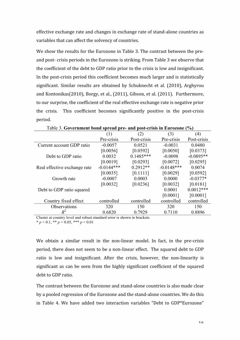
We show the results for the Eurozone in Table 3. The contrast between the pre-‐

and post-‐ crisis periods in the Eurozone is striking. From Table 3 we observe that

the coefficient of the debt to GDP ratio prior to the crisis is low and insignificant.

In the post-‐crisis period this coefficient becomes much larger and is statistically

significant. Similar results are obtained by Schuknecht et al. (2010), Arghyrou

and Kontonikas(2010), Borgy, et al., (2011), Gibson, et al. (2011). Furthermore,

to our surprise, the coefficient of the real effective exchange rate is negative prior

the crisis. This coefficient becomes significantly positive in the post-‐crisis

period.

Table 3. Government bond spread pre- and post-crisis in Eurozone (%) (1) (2) (3) (4) Pre-crisis Post-crisis Pre-crisis Post-crisis

Current account GDP ratio -0.0057 0.0521 -0.0031 0.0480 [0.0056] [0.0592] [0.0050] [0.0373]

Debt to GDP ratio 0.0032 0.1485*** -0.0098 -0.0895** [0.0019] [0.0293] [0.0072] [0.0295]

Real effective exchange rate -0.0144*** 0.2912** -0.0148*** 0.0074 [0.0035] [0.1111] [0.0029] [0.0592]

Growth rate -0.0007 0.0003 0.0000 -0.0377* [0.0032] [0.0236] [0.0032] [0.0181]

Debt to GDP ratio squared 0.0001 0.0012*** [0.0001] [0.0001]

Country fixed effect controlled controlled controlled controlled Observations 320 150 320 150

R2 0.6820 0.7929 0.7110 0.8896 Cluster at country level and robust standard error is shown in brackets. * p < 0.1, ** p < 0.05, *** p < 0.01

We obtain a similar result in the non-‐linear model. In fact, in the pre-‐crisis

period, there does not seem to be a non-‐linear effect. The squared debt to GDP

ratio is low and insignificant. After the crisis, however, the non-‐linearity is

significant as can be seen from the highly significant coefficient of the squared

debt to GDP ratio.

The contrast between the Eurozone and stand-‐alone countries is also made clear

by a pooled regression of the Eurozone and the stand-‐alone countries. We do this

in Table 4. We have added two interaction variables “Debt to GDP*Eurozone”

17

and “Real effective exchange rate* Eurozone”. The “Debt to GDP*Eurozone”

measures the degree to which the debt to GDP ratio affects the Eurozone spreads

differently from the stand-‐alone countries. The “Real effective exchange rate*

Eurozone” measures the degree to which the real effective exchange rate affects

the Eurozone spreads differently from the stand-‐alone countries. The results of

table 4 confirm the previous results. The Debt to GDP and the real effective

exchange rate are much stronger and significant variables in the Eurozone than

in the stand-‐alone countries especially in the post-‐crisis period. The stand-‐alone

countries seem to be able to “get away with murder” and still not be disciplined

by financial markets.

Table 4. Government bond spread in “Stand-alone” countries and Eurozone (%) (1) (2) (3) Total sample Pre-crisis Post-crisis Current account GDP ratio 0.0091 -0.0154* 0.0002 [0.0243] [0.0087] [0.0221] Debt to GDP ratio 0.0144* 0.0170 0.0176*** [0.0078] [0.0137] [0.0053] Debt to GDP ratio*Eurozone 0.0711*** -0.0135 0.1367*** [0.0185] [0.0137] [0.0314] Real effective exchange rate 0.0123 0.0040 0.0205*** [0.0122] [0.0150] [0.0071] Real effective exchange rate*Eurozone

0.0240 -0.0193 0.2742**

[0.0235] [0.0152] [0.1109] Growth rate -0.0289 0.0028 0.0004 [0.0269] [0.0154] [0.0107] Exchange rate against euro -0.0075 -0.0032 -0.0038* [0.0082] [0.0111] [0.0021] Country fixed effect controlled controlled controlled Observations 893 608 285 R2 0.7631 0.9222 0.8440 Cluster at country level and robust standard error is shown in brackets. * p < 0.1, ** p < 0.05, *** p < 0.01

To summarize, we find a great contrast between the Eurozone and the stand-‐

alone countries. In the former, we detected a significant increase in the effect of

the debt to GDP ratio and real effective exchange rate on the spreads since 2008.

Such an increase is completely absent in the stand-‐alone countries. Second, there

appears to be significant departures of the spreads from their fundamental

values in the Eurozone countries after the start of the crisis, suggesting that time

18

dependent movements in market sentiments become important. This does not

seem to be observed in the stand-‐alone countries. We analyze these time

dependent departures in the next section

6. Introducing time dependency In order to measure the importance of time dependent effects on the spreads, we

introduce time dependency in the basic fixed effect model. In the non-‐linear

specification this yields:

𝐼!" = 𝛼 + 𝑧 ∗ 𝐶𝐴!" + 𝛾! ∗ 𝐷𝑒𝑏𝑡!" + µμ ∗ 𝑅𝐸𝐸!" + 𝛿 ∗ 𝐺𝑟𝑜𝑤𝑡ℎ!" + 𝛾! ∗ (𝐷𝑒𝑏𝑡!")! +𝛼! + 𝛽! + 𝑢!"

where 𝛽! is the time dummy variable. This measures the time effects that are

unrelated to the fundamentals of the model or (by definition) to the fixed effects.

If significant, it shows that the spreads move in time unrelated to the

fundamentals forces driving the yields.

We estimated this model for both the stand-‐alone and the Eurozone countries. In

addition, we estimated the model separately for two subgroups of the Eurozone,

i.e. the core and the periphery7. The results are shown in Table 5. The contrast

between stand-‐alone and Eurozone countries is striking. The effect of the time

variable in the stand-‐alone countries is weak. In the Eurozone we detect some

increasing positive time effect since 2010Q2. Noticeably there exist some

significant and positive time effects from 2010Q4 to 2011Q3 in the periphery of

the Eurozone. Thus, during the post crisis period the spreads in the peripheral

countries of the Eurozone were gripped by surges that were independent from

the underlying fundamentals.

7 Chow test shows a split between the new and early members. Core Eurozone = Austria, Belgium, France, Finland, Italy, Netherlands. Periphery: Ireland, Greece, Portugal and Spain.

19

Table 5. Long-term government bond rate spread (%) with time component

Stand-alone Eurozone Core Eurozone Periphery Current account GDP ratio -0.0192 0.0628 -0.0099 0.0381

Debt to GDP ratio -0.0185 -0.0538* -0.0610* -0.0619* Exchange rate against euro 0.0004 --- --- ---

Real effective exchange rate 0.0061 0.0140 0.0647** 0.0040 Debt to GDP ratio squared 0.0001*** 0.0008*** 0.0004* 0.0008**

Growth rate -0.0156 -0.1311*** 0.0032 -0.0958** 2000Q2 -0.0727 0.0611 0.0910 0.0193 2000Q3 -0.1302 0.0584 0.1503 -0.0712 2000Q4 -0.1634 0.2963** 0.2339 0.2657 2001Q1 -0.1998 0.1016 0.0641 0.1505 2001Q2 -0.1719 0.0257 0.1417 0.1176 2001Q3 -0.1283 -0.0626 0.1045 0.1167 2001Q4 -0.0917 -0.1534 0.0391 -0.0528 2002Q1 -0.1860 -0.3177 -0.0050 -0.0490 2002Q2 -0.2289 -0.1372 -0.0787 -0.0090 2002Q3 -0.1954 -0.2080 -0.1570** -0.0320 2002Q4 -0.2109 -0.2013 -0.1899** -0.2181 2003Q1 -0.1293 -0.2899 -0.3855*** -0.2018 2003Q2 -0.1446 -0.4147 -0.4337*** -0.2405 2003Q3 -0.0572 -0.3902 -0.4487*** -0.2557 2003Q4 -0.0967 -0.1980 -0.4858*** -0.1223 2004Q1 -0.1449 -0.2706 -0.5721** -0.1840 2004Q2 0.0033 -0.2046 -0.4480** -0.1935 2004Q3 -0.0694 -0.1713 -0.4659*** -0.2011 2004Q4 -0.0130 -0.0910 -0.5179*** -0.2230 2005Q1 0.0154 -0.2525 -0.6403*** -0.2485 2005Q2 0.0765 -0.2224 -0.4970*** -0.2186 2005Q3 0.1119 -0.1873 -0.4493*** -0.2655 2005Q4 0.1148 -0.1272 -0.4063*** -0.3985 2006Q1 0.0329 -0.0187 -0.4225*** -0.1922 2006Q2 -0.0286 -0.0578 -0.4351*** -0.2715 2006Q3 -0.0532 -0.0115 -0.4827*** -0.2137 2006Q4 -0.0466 0.0271 -0.4628*** -0.3426 2007Q1 -0.1721 0.0763 -0.4869*** -0.2271 2007Q2 -0.2045 0.0190 -0.4938*** -0.3035 2007Q3 -0.1819 0.0751 -0.4566** -0.2175 2007Q4 -0.2268 0.2463 -0.4912*** -0.1006 2008Q1 -0.2477 0.0401 -0.4945** -0.2722 2008Q2 -0.3392 0.0542 -0.5076** -0.2267 2008Q3 -0.5108* 0.0267 -0.4120** -0.2427 2008Q4 -0.3500 -0.0832 0.0357 -0.1909 2009Q1 -0.3756 -0.2135 0.2244 0.2389 2009Q2 -0.2986 -0.7676 -0.0513 -0.5053 2009Q3 -0.2176 -1.1624* -0.2843 -1.1298 2009Q4 -0.1244 -0.9878* -0.3020 -0.9887 2010Q1 -0.0243 -0.5864 -0.2375 -0.6235 2010Q2 0.1200 0.0326 0.1081 0.4846 2010Q3 0.0555 0.3226 0.1343 1.2979 2010Q4 0.0140 0.5379 0.1856 1.7012** 2011Q1 -0.1918 0.4821 0.1714 1.5040** 2011Q2 -0.3508** 1.0023 0.1524 3.0390** 2011Q3 -0.1806 1.4995* 0.7036* 3.5781*

Country fixed effect controlled Yes Yes Yes Yes Observations 423 470 282 188

R2 0.9339 0.8581 0.8287 0.9566 Note: Cluster at the country level and robust standard error is shown in the brackets. * p < 0.1, ** p < 0.05, *** p < 0.01

20

Finally we plot the time effects obtained from table 5 in Figure 9. This suggests

that especially in the periphery “departures” occurred in the spreads, i.e. an

increase in the spreads that cannot be accounted for by fundamental

developments, in particular by the changes in the debt to GDP ratios during the

crisis.

This result can also be interpreted as follows. Before the crisis the markets did

not see any risk in the peripheral countries’ sovereign debt. As a result they

priced the risks in the same way as the risk of core countries’ sovereign debt.

After the crisis, spreads of the peripheral countries increased dramatically and

independent from observed fundamentals. This suggests that the markets were

gripped by negative sentiments and tended to exaggerate the default risks. Thus,

mispricing of risks (in both directions) seems to have been an endemic feature in

the Eurozone.

Figure 9: Time variable, Eurozone and stand-‐alone Stand-‐alone Eurozone

Core Eurozone Peripheral Eurozone

21

7. Conclusion

One important empirical puzzle concerning the sovereign debt crisis is that it

erupted in the Eurozone despite the fact that the fiscal position of the Eurozone

as a whole was better than the fiscal position of countries like the US and the UK

that were left unscathed by the crisis. True Greece had accumulated

unsustainable debt and deficit levels, but the other Eurozone countries that were

hit by the debt crisis were not in a worse fiscal position than the US and the UK.

Our explanation of this puzzle is along the lines developed in De Grauwe(2011),

who argues that government bond markets in a monetary union are more fragile

and more susceptible to self-‐fulfilling liquidity crises than in stand-‐alone

countries. The reason is that as the latter issue their own money, they give a

guarantee to bondholders that the cash will always be available at maturity. The

members of a monetary union cannot give such a guarantee and as a result are

more vulnerable to negative market sentiments that in a self-‐fulfilling way can

create a liquidity crisis. The purpose of this paper was to develop a test of this

fragility hypothesis.

On the whole we confirm this hypothesis. We found evidence that a large part of

the surge in the spreads of the PIGS countries during 2010-‐11 was disconnected

from underlying increases in the debt to GDP ratios, and was the result of time

dependent negative market sentiments that became very strong since the end of

2010. The stand-‐alone countries in our sample have been immune from these

liquidity crises and weathered the storm without the increases in the spread.

We also found evidence that after years of neglecting high debt to GDP ratios,

investors became increasingly worried about the high debt to GDP ratios in the

Eurozone, and reacted by raising the spreads. No such worries developed in

stand-‐alone countries despite the fact that debt to GDP ratios were equally high

and increasing in these countries. This result can also be said to validate the

fragility hypothesis, i.e. the markets appear to be less tolerant towards large debt

to GDP ratios in the Eurozone than towards equally large ratios in the stand-‐

alone countries.

Thus, the story of the Eurozone is also a story of self-‐fulfilling debt crises, which

in turn lead to multiple equilibria. Countries that are hit by a liquidity crisis are

22

forced to apply stringent austerity measures that force them into a recession,

thereby reducing the effectiveness of these austerity programs. There is a risk

that the combination of high interest rates and deep recessions turn the liquidity

crisis into a solvency crisis.

In a world where spreads are tightly linked to the underlying fundamentals such

as the debt to GDP ratio, the only option the policy makers have in reducing the

spreads is to improve the fundamentals. This implies measures aimed at

reducing the debt burden. If, however, there can be a disconnection between the

spreads and the fundamentals, a policy geared exclusively towards affecting the

fundamentals (i.e. reducing the debt burden) will not be sufficient. In that case

policy makers should also try to stop countries from being driven into a bad

equilibrium. This can be achieved by more active liquidity policies by the ECB

that aim at preventing a liquidity crisis from leading to a self-‐fulfilling solvency

crisis (Wyplosz(2011) and De Grauwe(2011)).

23

References

Arghyrou, M. and Kontonikas, A., (2010), The EMU sovereign-‐debt crisis:

Fundamentals, expectations and contagion, Cardiff Economics Working Papers, E2010/9

Attinasi, M., Checherita, C., and Nickel, C., (2009), What explains the surge in Euro area sovereign spreads during the financial crisis of 2007-‐09? ECB working paper, NO 1131, December

Boehmer, E. and W.L. Megginson, 1990, "Determinants of Secondary Market Prices for Developing Country Syndicated Loans," Journal of Finance 45-5, 1,517-1,540.

Blanchard, O., (2011), Four Hard Truths, VoxEU, http://www.voxeu.org/index.php?q=node/7475

Caceres, C., Guzzo, V., and Segoviano, M., (2010), Sovereign Spreads: Global Risk Aversion, Contagion or Fundamentals?, IMF working paper, May

Calvo, Guillermo (1988): Servicing the Public Debt: The Role of Expectations, American Economic Review, Vol. 78, No. 4, pp. 647-‐661

Caporale, G., and Girardi, A., (2011), Fiscal Spillovers in the Euro Area, Discussion Paper, 1164, DIW, Berlin, October.

Corsetti, G.C., and Dedola, L., (2011), Fiscal Crises, Confidence and Default. A Bare-‐bones Model with Lessons for the Euro Area, unpublished, Cambridge.

De Grauwe, P., (2011), The Governance of a Fragile Eurozone, Economic Policy, CEPS Working Documents, May, http://www.ceps.eu/book/governance-‐fragile-‐eurozone

De Grauwe, P., (2011), The ECB as a lender of last resort, VoxEU, October, http://www.voxeu.org/ index.php?q=node/6884

Diamond DW, and Dybvig PH (1983). "Bank runs, deposit insurance, and liquidity". Journal of Political Economy 91 (3): 401–419

Eaton, J. and M. Gersovitz, 1981, "Debt with Potential Repudiation: Theoretical and Empirical Analysis," Review of Economic Studies 48, 289-309.

Eaton, J., M. Gersovitz, and J. E. Stiglitz, 1986, “ The Pure Theory of Country Risk,” European Economic Review, 30, June, 481-513.

Edwards, S., 1984, ”LDC Foreign Borrowing and Default Risk:An Empirical Investigation,:1976-1980,” American Economic Review, 74, September, 726-734.

Edwards, S., 1986, “The Pricing of Bonds and Bank Loans in International Markets: An Empirical Analysis of Developing Countries’Foreign Borrowing, European Economiv Review, vol 30, 565-589.

Eichengreen, B. and A. Mody, 2000, "Lending Booms, Reserves and the Sustainability of Short- Term Debt: Inferences from the Pricing of Syndicated Bank Loans," Journal of Development Economics 63, 5-44.

Eichengreen, B., Hausmann, R., Panizza, U., (2005), “The Pain of Original Sin”, in Eichengreen, B., and Hausmann, R., Other people’s money: Debt denomination

24

and financial instability in emerging market economies, Chicago University Press.

Gerlach, S., Schulz, G., and Wolff, W., (2010), Banking and Sovereign Risk in the Euro Area, mimeo, Deutsche Bundesbank.

Gibson, H., G. Hall G. and Tavlas, G., (2011 March), The Greek Financial Crisis: Growing Imbalances and Sovereign Spreads, , working paper, Bank of Greece.

Gros, D., (2011), A simple model of multiple equilibria and default, mimeo, CEPS

Kindleberger, (2005), Manias, Panics, and Crashes: A History of Financial Crises (Palgrave Macmillan , 5th edition)

McKinnon, R., and Goyal, (2003), Japan’s Negative Risk Premium in Interest Rates: The Liquidity Trap and Fall in Bank Lending” The World Economy March 2003, pp 339-‐364

Min, H., (1999), Determinants of Emerging Market Bond Spread: Do Economic Fundamentals Matter?, World Bank, http://elibrary.worldbank.org/content/workingpaper/10.1596/1813-‐9450-‐1899

Obstfeld, M., (1986), 'Rational and self-‐fulfilling balance-‐of-‐payments crises'. American Economic Review 76 (1), pp. 72-‐81.

Schuknecht, L., von Hagen, J., and Wolswijk, G., (2010), Government Bond Risk Premiums in the EU Revisited the impact of the financial crisis, ECB working paper No 1152, 2010 February

Wyplosz, C., (2011), They still don’t get it, VoxEU, http://www.voxeu.org/ index.php?q=node/6845

25

APPENDIX: A MODEL OF GOOD AND BAD EQUILIBRIA

In this section we present a very simple model illustrating how multiple

equilibria can arise. The starting point is that there is a cost and a benefit of

defaulting on the debt, and that investors take this calculus of the sovereign into

account. We will assume that the country involved is subject to a shock, which

takes the form of a decline in government revenues. The latter may be caused by

a recession, or a loss of competitiveness. We’ll call this a solvency shock. The

higher this shock the greater is the loss of solvency. We concentrate first on the

benefit side. This is represented in Figure A1. On the horizontal axis we show

the solvency shock. On the vertical axis we represent the benefit of defaulting.

There are many ways and degrees of defaulting. To simplify we assume this

takes the form of a haircut of a fixed percentage. The benefit of defaulting in this

way is that the government can reduce the interest burden on the outstanding

debt. As a result, after the default it will have to apply less austerity, i.e. it will

have to reduce spending and/or increase taxes by less than without the default.

Since austerity is politically costly, the government profits from the default.

A major insight of the model is that the benefit of a default depends on whether

this default is expected or not. We show two curves representing the benefit of a

default. BU is the benefit of a default that investors do not expect to happen,

while BE is the benefit of a default that investors expect to happen. Let us first

concentrate on the BU curve. It is upward sloping because when the solvency shock increases, the benefit of a default for the sovereign goes up. The reason is

that when the solvency shock is large, i.e. the decline in tax income is large, the

cost of austerity is substantial. Default then becomes more attractive for the

sovereign. We have drawn this curve to be non-‐linear, but this is not essential for

the argument. We distinguish three factors that affect the position and the

steepness of the BU curve:

• The initial debt level. The higher is this level, the higher is the benefit of a

default. Thus with a higher initial debt level the BU curve will rotate upwards.

26

• The efficiency of the tax system. In a country with an inefficient tax system, the

government cannot easily increase taxation. Thus in such a country the

option of defaulting becomes more attractive. The BU curve rotates upwards.

• The size of the external debt. When external debt takes a large proportion of

total debt there will be less domestic political resistance against default,

making the latter more attractive (the BU curve rotates upwards).

Figure A1: The benefits of default after a solvency shock B

We now concentrate on the BE curve. This shows the benefit of a default when

investors anticipate such a default. It is located above the BU curve for the following reason. When investors expect a default, they will sell government

bonds. As a result, the interest rate on government bonds increases. This raises

the government budget deficit requiring a more intense austerity program of

spending cuts and tax hikes. Thus, default becomes more attractive. For every

solvency shock, the benefits of default will now be higher than they were when

the default was not anticipated.

BU

Solvency shock

BE

27

We now introduce the cost side of the default. The cost of a default arises from

the fact that, when defaulting, the government suffers a loss of reputation. This

loss of reputation will make it difficult for the government to borrow in the

future. We will make the simplifying assumption that this is a fixed cost. We now

obtain Figure A2 where I present the fixed cost (C) with the benefit curves.

Figure A2: Cost and benefits of default after a solvency shock B

We now have the tools to analyze the equilibrium of the model. We will

distinguish between three types of solvency shocks, a small one, an intermediate

one, and a large one. Take a small solvency shock: this is a shock S < S1 (This

could be the shocks that Germany and the Netherlands experienced during the

debt crisis). For this small shock the cost of a default is always larger than the

benefits (both of an expected and an unexpected default). Thus the government

will not want to default. When expectations are rational investors will not expect

a default. As a result, a no-‐default equilibrium can be sustained.

Let us now analyze a large solvency shock. This is one for which S > S2. (This

could be the shock experienced by Greece). For all these large shocks we observe

that the cost of a default is always smaller than the benefits (both of an expected

BU BE

C

S1 S2

28

and an unexpected default). Thus the government will want to default. In a

rational expectations framework, investors will anticipate this. As a result, a

default is inevitable.

We now turn to the intermediate case: S1 < S < S2. (This could be the shocks that

Ireland, Portugal and Spain experienced). For these intermediate shocks I obtain

an indeterminacy, i.e. two equilibria are possible. Which one will prevail only

depends on what is expected. To see this, suppose the solvency shock is S’ (see

Figure A3). In this case there are two potential equilibria, D and N. Take point D.

In this case investors expect a default (D is located on the BE line). This has the

effect of making the benefit of a default larger than the cost C. Thus, the

government will default. D is an equilibrium that is consistent with expectations.

But point N is an equally good candidate to be an equilibrium point. In N,

investors do not expect a default (N is on the BU line). As a result, the benefit of a

default is lower than the cost. Thus the government will not default. It follows

that N is also an equilibrium point that is consistent with expectations.

Figure A3: Good and bad equilibria

B

BU

BE

C

S1 S2

D

S’

N

29

Thus we obtain two possible equilibria, a bad one (D) that leads to default, a

good one (N ) that does not lead to default. Both are equally possible. The

selection of one of these two points only depends on what investors expect. If the

latter expect a default, there will be one; if they do not expect a default there will

be none. This remarkable result is due to the self-‐fulfilling nature of expectations.

Since there is a lot of uncertainty about the likelihood of default, and since

investors have very little scientific foundation to calculate probabilities of default

(there has been none in Western Europe in the last 60 years), expectations are

likely to be driven mainly by market sentiments of optimism and pessimism.

Small changes in these market sentiments can lead to large movements from one

type of equilibrium to another.

The possibility of multiple equilibria is unlikely to occur when the country is a

stand-‐alone country, i.e. when it can issue sovereign debt in its own currency.

This makes it possible for the country to always avoid outright default because

the central bank can be forced to provide all the liquidity that is necessary to

avoid such an outcome. This has the effect that there is only one benefit curve. In

this case the government can still decide to default (if the solvency shock is large

enough). But the country cannot be forced to do so by the whim of market

expectations

Preliminarydraft* SELF2FULFILLINGCRISESIN*THEEUROZONE ... · % 2% * 1. Introduction* The financial%...

Documents

Transcript of Preliminarydraft* SELF2FULFILLINGCRISESIN*THEEUROZONE ... · % 2% * 1. Introduction* The financial%...

Preliminarydraft* SELF2FULFILLINGCRISESINTHEEUROZONE ... · % 2% 1. Introduction* The financial%...

Transcript of Preliminarydraft* SELF2FULFILLINGCRISESINTHEEUROZONE ... · % 2% 1. Introduction* The financial%...