PRELIMINARY RESULTS OF A LOW-COST GPS-BASEDGLACIER MONITORING SYSTEM: TRAPRIDGE GLACIER,

YUKON TERRITORY, CANADA.

by

Rob A. Eso

A THESIS SUBMITTED IN PARTIAL FULFILMENT OFTHE REQUIREMENTS FOR THE DEGREE OF

BACHELOR OF APPLIED SCIENCES

in

GEOLOGICAL ENGINEERINGFaculty of Applied Science

Geological Engineering Program

We accept this thesis as conforming tothe required standard

THE UNIVERSITY OF BRITISH COLUMBIAAPRIL, 2004

Abstract

A low-cost GPS system has been designed and built at the University of British

Columbia, and is specifically designed to operate in the harsh conditions typical

of glaciated environments. Two GPS prototypes were deployed on the Trapridge

Glacier research site in the Yukon Territory, Canada. Results from 2002–2003

are post-processed, and comparisons with net movement estimates of Trapridge

Glacier derived using traditional surveying methods are made. Results indi-

cate that the GPS derived net movement estimates are in agreement with those

of a traditional optical survey. A least-squares estimate is used to fit a two-

velocity linear model to Trapridge Glacier, showing that the glacier exhibits a

summer/spring velocity of 17.6 m a−1, and a winter velocity mode of between

0.0–6.9 m a−1. Experience from this field season is analyzed, and recommenda-

tions for the future development of the GPS system are discussed. Design and

fabrication details, as well as detailed circuit board, schematics and part lists for

the prototype units are provided.

ii

Acknowledgements

This thesis presents the work done by several people over since the summer of

2002. Foremost, I would like to thank Garry Clarke for supervising this thesis

and for being the driving force behind the development of the GPS system. I’d

like to thank David Jones, who completed most of the electronic design and

programming for the GPS, and the Trapridge Glacier field crew consisting of Tom-

Pierre Frappe-Seneclauze, David King, and Jessica Logher for their help in all

aspects of the project. I am grateful to thank Barry Narod for graciously agreeing

to solder the surface mount components on the 2003 prototype on very short

notice. The UBC Earth and Ocean Sciences Machine Shop, Bryon Cranston,

Michael St. Pierre, Doug Polson, and Ray Rodway accommodated several last

minute fabrication requests which were required for completion of the project.

Lastly, I’d like to thank Andy Williams, Lance Goodwin, and Sian Williams of

the Arctic Institute of North America for providing two years of accommodation

on the lovely Kluane Lake, and for tossing the 2003 GPS prototype out of an

airplane.

Rob A. Eso

The University of British Columbia

April 2004

iii

Table of Contents

Abstract ii

Acknowledgements iii

List of Figures viii

List of Tables x

Chapter 1 Introduction 1

1.1 Thesis overview . . . . . . . . . . . . . . . . . . . . . . . . . . . . 2

Chapter 2 Literature Review 4

2.1 GPS surveys on Svalbard glaciers, Norway . . . . . . . . . . . . . 4

2.2 Comparison of ice velocities derived from satellite images and GPS 5

2.3 Precise point positioning using IGS orbit products . . . . . . . . . 6

2.4 Low-cost GPS volcano deformation monitoring . . . . . . . . . . 7

2.5 Automated motion and stream measurements . . . . . . . . . . . 8

2.6 General text books . . . . . . . . . . . . . . . . . . . . . . . . . . 9

Chapter 3 Study Area 10

3.1 Trapridge Glacier environment . . . . . . . . . . . . . . . . . . . . 11

3.1.1 Temperature . . . . . . . . . . . . . . . . . . . . . . . . . . 11

iv

3.1.2 Solar energy intensity . . . . . . . . . . . . . . . . . . . . . 12

3.2 Geological setting . . . . . . . . . . . . . . . . . . . . . . . . . . . 13

3.2.1 Trapridge Glacier physical geography . . . . . . . . . . . . 14

3.3 Current research at Trapridge Glacier . . . . . . . . . . . . . . . . 15

Chapter 4 GPS Theory 17

4.1 GPS satellite signals . . . . . . . . . . . . . . . . . . . . . . . . . 17

4.1.1 Selective availability . . . . . . . . . . . . . . . . . . . . . 18

4.2 Positioning concepts . . . . . . . . . . . . . . . . . . . . . . . . . 18

4.2.1 Differential carrier phase tracking . . . . . . . . . . . . . . 18

4.2.2 Pseudo-range positioning . . . . . . . . . . . . . . . . . . . 20

4.3 Error sources in GPS positioning . . . . . . . . . . . . . . . . . . 22

4.3.1 Satellite errors . . . . . . . . . . . . . . . . . . . . . . . . . 22

4.3.2 Propagation errors . . . . . . . . . . . . . . . . . . . . . . 23

4.3.3 Receiver errors . . . . . . . . . . . . . . . . . . . . . . . . 24

4.4 GPS surveying considerations . . . . . . . . . . . . . . . . . . . . 25

4.4.1 Visible satellites . . . . . . . . . . . . . . . . . . . . . . . . 25

4.4.2 Elevation cutoff mask . . . . . . . . . . . . . . . . . . . . . 26

Chapter 5 GPS Prototype 27

5.1 Hardware . . . . . . . . . . . . . . . . . . . . . . . . . . . . . . . 28

5.1.1 GPS receivers and antennas . . . . . . . . . . . . . . . . . 29

5.1.2 Power supply . . . . . . . . . . . . . . . . . . . . . . . . . 29

5.1.3 Microprocessor and memory . . . . . . . . . . . . . . . . . 30

5.1.4 Environmental enclosures and mounting hardware . . . . . 31

5.2 GPS prototype operation . . . . . . . . . . . . . . . . . . . . . . . 31

Chapter 6 Results 34

6.1 Receiver status and data collected . . . . . . . . . . . . . . . . . . 34

6.1.1 02GPS02 . . . . . . . . . . . . . . . . . . . . . . . . . . . . 35

6.1.2 02GPS03 . . . . . . . . . . . . . . . . . . . . . . . . . . . . 35

6.1.3 Damage to the prototypes . . . . . . . . . . . . . . . . . . 35

6.2 Unprocessed GPS positions . . . . . . . . . . . . . . . . . . . . . 36

6.3 Post-Processed results . . . . . . . . . . . . . . . . . . . . . . . . 39

6.3.1 Net glacier movement from GPS survey . . . . . . . . . . . 41

6.4 Net glacier movement from optical survey . . . . . . . . . . . . . 41

6.5 Annual velocity model for Trapridge Glacier . . . . . . . . . . . . 42

Chapter 7 Conclusions 44

Chapter 8 Recommendations for Further Work 46

8.1 GPS survey improvements and recommendations . . . . . . . . . 46

8.1.1 Processing software . . . . . . . . . . . . . . . . . . . . . . 47

8.2 Hardware improvements and recommendations . . . . . . . . . . . 48

8.2.1 Memory storage and transfer . . . . . . . . . . . . . . . . . 48

8.2.2 PCB design and component selection . . . . . . . . . . . . 49

8.2.3 PCB layout and mounting . . . . . . . . . . . . . . . . . . 50

8.2.4 Measurement of battery voltage and temperature . . . . . 51

8.3 Software improvements and recommendations . . . . . . . . . . . 51

Appendix A Visible Satellites at Trapridge Glacier 53

A.1 Trapridge Glacier . . . . . . . . . . . . . . . . . . . . . . . . . . . 53

A.2 North pole and Equator . . . . . . . . . . . . . . . . . . . . . . . 54

Appendix B Linearized GPS Solution 59

B.1 ECEF coordinate system . . . . . . . . . . . . . . . . . . . . . . . 61

Appendix C Trapridge Coordinate Transformation 62

C.1 Method . . . . . . . . . . . . . . . . . . . . . . . . . . . . . . . . 62

C.2 Results . . . . . . . . . . . . . . . . . . . . . . . . . . . . . . . . . 63

C.3 Applicability of Results . . . . . . . . . . . . . . . . . . . . . . . . 64

Appendix D GPS Printed Circuit Board 66

D.1 Part List . . . . . . . . . . . . . . . . . . . . . . . . . . . . . . . . 66

References 69

List of Figures

3.1 Trapridge Glacier study area . . . . . . . . . . . . . . . . . . . . . 10

3.2 Trapridge Glacier location . . . . . . . . . . . . . . . . . . . . . . 11

3.3 1999 temperature, logger #12603 . . . . . . . . . . . . . . . . . . 12

3.4 1999 battery voltage, logger #12603 . . . . . . . . . . . . . . . . . 13

3.5 Trapridge Glacier bulge evolution, 1980–1988 . . . . . . . . . . . . 15

4.1 Differential GPS . . . . . . . . . . . . . . . . . . . . . . . . . . . . 19

4.2 GPS standalone pseudo-range positioning . . . . . . . . . . . . . . 20

4.3 GPS satellite orbits . . . . . . . . . . . . . . . . . . . . . . . . . . 25

5.1 UBC prototype GPS receiver units . . . . . . . . . . . . . . . . . 27

5.2 2002 and 2003 GPS units . . . . . . . . . . . . . . . . . . . . . . . 28

5.3 GPS prototype operation flowchart . . . . . . . . . . . . . . . . . 32

6.1 Position of 2002 GPS receivers . . . . . . . . . . . . . . . . . . . . 34

6.2 Damage sustained by 02GPS02 . . . . . . . . . . . . . . . . . . . 36

6.3 02GPS02 unprocessed data . . . . . . . . . . . . . . . . . . . . . . 37

6.4 02GPS03 unprocessed data . . . . . . . . . . . . . . . . . . . . . 38

6.5 GPS data from September 5, 2002 . . . . . . . . . . . . . . . . . . 39

6.6 02GPS03 post-processed results . . . . . . . . . . . . . . . . . . . 40

viii

6.7 Two velocity model of Trapridge . . . . . . . . . . . . . . . . . . . 43

A.1 2 hour satellite coverage at Trapridge Glacier . . . . . . . . . . . . 55

A.2 11 hour satellite coverage at Trapridge Glacier . . . . . . . . . . . 56

A.3 Satellite coverage at the Equator . . . . . . . . . . . . . . . . . . 57

A.4 Satellite Coverage at the North Pole . . . . . . . . . . . . . . . . 58

C.1 Trapridge pseudo–UTM and WGS–84 survey points . . . . . . . . 63

D.1 2003 GPS Prototype Schematic . . . . . . . . . . . . . . . . . . . 67

D.2 2003 GPS prototype circuit board . . . . . . . . . . . . . . . . . . 68

List of Tables

4.1 Error sources in GPS surveying . . . . . . . . . . . . . . . . . . . 22

4.2 GPS error sources and RMS effect on position . . . . . . . . . . . 22

6.1 2002-2003 GPS displacement . . . . . . . . . . . . . . . . . . . . . 41

6.2 2002-2003 survey displacements . . . . . . . . . . . . . . . . . . . 42

7.1 Comparison of GPS and optical net movement . . . . . . . . . . . 44

C.1 Trapridge pseudo-UTM coordinates . . . . . . . . . . . . . . . . . 64

C.2 Trapridge WGS-84 coordinates . . . . . . . . . . . . . . . . . . . 64

C.3 Difference between Trapridge and WGS-84 . . . . . . . . . . . . . 64

D.1 Electrical component list for the 2003 GPS prototype. . . . . . . . 66

D.2 Other components for the 2003 GPS prototype. . . . . . . . . . . 66

x

1. Introduction

Traditionally, surveying done in glaciated environments have tracked glacier move-

ment through optical measurements. Theodolites and laser–range finders are

typically used to determine the distance and bering to survey prisms mounted

atop flow–maker poles inserted along a glaciers surface. Although accurate, this

method is logistically expensive, having to deal with the cost of a surveyor, place-

ment of survey prisms, and expensive surveying equipment. This method of opti-

cal surveying is incapable of operating in weather conditions with poor visibility,

and is often limited to studying glacier movement during warmer months of the

year; as colder periods can be quite inhospitable. Large glaciers and ice sheets

are also difficult to survey optically, as the areas of interest may not all be vis-

ible from a single location. Some methods have been developed to track glacier

movement during the winter, such as using cameras to photograph flow–marker

poles during the winter months Harrison et al. (1989).

The Navstar Global Positioning System (GPS) has revolutionized the way

in which surveying is done in the scientific community. A constellation of 24 orbit-

ing satellites allows the precise determination of geographic coordinates anywhere

on the planet, and has opened up new possibilities for tracking of glacial move-

ment. GPS systems have been involved in glacier research for several years (Eiken

et al., 1997, Frezzotti et al., 1998). The GPS systems typically deployed have

been able to achieve centimeter accuracy, and have provided a robust method of

tracking glacier movement. However, such systems can cost over $20,000 USD

per installation site. The risk of damaging expensive GPS equipment has often

resulted in shorter, campaign style surveys being undertaken to study glaciers;

not often are continuous movement records obtained. The need for a low–cost

1

movement monitoring system is not restricted to glaciology. A low–cost volcano

deformation system is developed by Janssen et al. (2002), with an installation

cost of $3000 USD per site.

The goal of this project was to develop a low–cost GPS receiver system

using inexpensive, off–the–shelf electronic components, and to demonstrate the

feasibility of such low–cost systems to operate year–round in difficult glaciated

environments. The resulting design will be available to the scientific community

for further development, and incorporation into research projects.

The GPS system described in this thesis presents an inexpensive way to

track year–round glacial movement at an installation cost of approximately $500

USD per site. These GPS systems can then be installed on the glaciers’ surface

and used to track year-round movement. This will allow several sites on the

glacier surface to be monitored autonomously throughout the year.

1.1 Thesis overview

This thesis discusses the design and fabrication of a prototype GPS deployed

on the Trapridge Glacier in July 2002. Data collected from July 2002 to July

2003 is processed and compared with net movement measurements made from

an optical survey. GPS prototypes made in 2003 are also discussed, however

no data from these units is analyzed. A variety of scientific research papers are

reviewed in Chapter 2. Papers dealing with both GPS theory, and those dealing

with the application of GPS to specific research projects in both glaciology and

volcanology are discussed. Chapter 3 outlines the environmental climate of the

Trapridge Glacier, and details how the environment creates difficulties in employ-

ing an automated GPS system. The geological setting and physical geography

2

of Trapridge Glacier are also discussed. The basic concepts of GPS system are

reviewed in Chapter 4. The theory of determining a geographic position from

satellite signals is discussed. Various aspects of the GPS surveying system such

as error sources and the effects of the satellite constellation geometry are also

examined. Chapter 5 reviews the design of the GPS prototypes developed at the

University of British Columbia, and overviews the components selected for the

device. The operating methodology for the devices is also discussed. Results ob-

tained from the GPS prototypes survey of Trapridge Glacier from July 2002 until

July 2003 are discussed in Chapter 6. A summary of how the GPS prototypes

preformed during the winter is made, and data collected by two GPS prototypes

installed on the glacier during this period is processed and the net movement

of Trapridge Glacier is estimated. A comparison of the net movement amounts

derived from GPS surveying and optical surveying is made, and a GPS derived

annual velocity model for Trapridge Glacier is proposed. Recommendations for

Further work outlines directions for future research and development of the low–

cost GPS system, and improvements in the survey setup. A detailed part list,

schematic, and circuit board from the 2003 GPS prototype are provided in the

appendix.

3

2. Literature Review

Although the papers discussed in this chapter deal mainly with more expen-

sive dual-frequency geodetic grade GPS receiver systems, and involve analysis of

the carrier-phase observation, they serve to outline the processing strategies and

methodologies employed in GPS surveying. They also provide some background

into the application of GPS surveys in harsh climatic environments which are the

norm for glaciology.

2.1 GPS surveys on Svalbard glaciers, Norway

A multi-year GPS survey was undertaken on several of the glaciers in Svalbard,

a territory of Norway. Traditional surveying methods were difficult to apply on

the large glaciers of Svalbard, roughly 80 km in length. GPS was used to create

surface profiles and to monitor several stationary sites (Eiken et al., 1997). Data

was collected over a four year period from 1991 to 1995 using dual frequency GPS

receivers. Static GPS sites were drilled into the glacier surface, while profiles

were generated using snowmobile mounted GPS receivers. The static locations

collected between 1 to 2 hours of data at a time and were able to track elevation

changes over the four year period. Resulting accuracies were under 1 centimeter.

Eiken et al. concludes that GPS is a suitable replacement for traditional surveying

techniques used to measure glacier mass balance. They also conclude that with

long enough collection periods and advanced software processing, the difficulties

of GPS surveying in high northern latitudes can be overcome provided that more

than five satellites are visible for long periods of time.

4

2.2 Comparison of ice velocities derived from satellite im-

ages and GPS

Ice motion estimates are crucial for determining the mass balance of the Antarctic

ice sheet, yet logistical problems and challenging environmental conditions make

surveying of Antarctica’s ice sheets and glaciers difficult. It has been shown that

ice velocities can be inferred from synthetic aperture radar (SAR) satellite images,

but there has been very little comparison with SAR results to GPS or traditional

optical surveys. Multi-year GPS data has been used to compare Antarctic ice-

sheet velocities derived from GPS surveying and SAR images (Frezzotti et al.,

1998). Inferring the velocity from SAR images requires tracking features on the

ice surface which are large enough to be visible in the SAR images. The Dry-

galski Ice Tongue was monitored using 73 points; the velocity tracked using the

Landsat–1 multispectral scanner and Landsat thematic mapper. Using these im-

ages, the average velocity of the Drygalski Ice Tongue was found to be 700 m a−1.

GPS measurements made at various times between 1989 and 1994 were used to

determine average ice velocities at similar points in time of those in the SAR

images.

Comparison of similar points using both the GPS and SAR derived av-

erage ice velocities were found to agree to within 15–20 m a−1 on the average,

with differences of up to 70 m a−1 at some locations. Frezzotti et al. conclude

that estimated errors of ± 15–20 m a−1 for SAR velocities could be quite large

for small outlet glaciers exhibiting velocities of 100–200 m a−1, but are of less

significance for most of the major outlet glaciers in Antarctica with velocities of

400–1000 m a−1. This suggests that although ice velocities can be inferred from

5

satellite images on large, fast moving glaciers, for smaller non-Antarctic glaciers

exhibiting flow velocities of 10–30 m a−1 it may be difficult or impossible to obtain

estimates of movement from satellite images alone.

2.3 Precise point positioning using IGS orbit products

As part of the procedure to determine the receiver’s geographic coordinates, the

GPS satellite positions in space must be known with a high level of accuracy.

These positions are transmitted continually by each satellite, but small pertur-

bations into the satellite orbits can be introduced. It is also required that all the

GPS satellites be synchronized to the same time system. Although atomic clocks

on board the satellites keep time to a very high degree of accuracy, there is still

a small clock drift between the different satellites. To synchronize all satellites

to a common time system all satellite clocks get updated at regular intervals

from ground stations. The International GPS Service (IGS) tracks all satellites

and publishes accurate descriptions of the satellite positions and clock drift free

through the internet.

Users in the GPS and geodetic communities have adopted as common pro-

cedure the use of IGS orbital products to achieve sub-centimeter to sub-millimeter

accuracy. This currently applies differential positioning concepts in which the ob-

servations from a minimum of two receivers are combined; the unknown receiver

position is then determined relative to a fixed reference station. This method is

popular and has been successfully applied in various applications. A significant

drawback of differential positioning is that it requires all observations be synchro-

nized between all receiving stations. A method has been outlined to make use

6

of the IGS final orbital products1 to perform corrections to undifferentiated dual

frequency pseudo-range and carrier phase observations at a stand-alone location

(Heroux et al., 2001). In doing so, they achieve centimeter level accuracy at a

static location without the hindrance of a base station. However, to achieve such

a high degree of accuracy it is necessary to apply various correction terms to the

data. These include solid earth tides, ocean loading, and variations of the Earth

rotation parameters (such as pole position and precession). The paper demon-

strates the feasibility of using single site GPS measurements to obtain accurate

geographic position estimates with centimeter scale accuracy using undifferenti-

ated GPS observations. This paper also serves to highlight the importance of

post-processing GPS data with information such as the IGS final orbits.

2.4 Low-cost GPS volcano deformation monitoring

Accurate knowledge of the deformation of volcanos is necessary for both predic-

tive and scientific information about active volcanos. However, the harsh and

sometimes dangerous environments of active volcanos do not make them good

candidates for traditional surveying methods. Autonomous GPS sites constantly

measuring the active deformation would be an ideal solution. A low cost GPS

system was placed in Indonesia and evaluated as a system for remote volcano

deformation monitoring (Janssen et al., 2002). A method of combining high ac-

curacy geodetic GPS receivers along a perimeter of the volcano combined with

low cost single frequency GPS receivers placed on the volcano is outlined in the

paper.

1IGS orbit products are released at several periods after the initial satellite observation ismade with increasing accuracy. The final orbital product is the most accurate, and is normallyavailable within two weeks of the observation date. http://igscb.jpl.nasa.gov/.

7

The low cost single frequency GPS receivers were placed at various po-

sitions on the volcano and transmitted data to a base station through a VHF

radio connection for processing. The outer GPS network was used to generate

correction terms which were applied to the observations from the inner network

on the volcano. The systems used 8086 PC based systems which ran a DOS

based operating system and used 12V batteries charged by solar panels. The

base station was powered by an AC power system with an uninterrupted power

supply. An installation cost of $3000 USD per site was achieved for the entire

survey.

However, it was found that the PC based systems suffered from memory

leaks, and that the DOS based software eventually stopped working due to mem-

ory loss. A microchip based system was recommended to replace the PC system

as it has more capabilities for real time operations. Environmental problems were

also an issue for the survey. Sulphur gas from the volcano seriously corroded the

units, while strong winds destroyed one observation site. It was found that high

level of noise attributed to ionospheric phenomenon prevented successful post-

processing of the inner GPS network data and thus no information about the

volcano deformation could be inferred from the GPS data (Janssen et al., 2002).

2.5 Automated motion and stream measurements

To attempt to reconstruct year–long glacier motion from the Fels and Black

Rapids glaciers in Alaska, an automated method for taking pictures of survey

poles was developed (Harrison et al., 1989). This novel method involved focusing

photographic cameras at survey poles and automatically exposing the film at set

time intervals using a mechanical device. This method was highly susceptible to

8

weather and visibility. This serves to highlight the lengths to which glaciologists

were willing to go to recover year round movement records of the glaciers they

were studying.

2.6 General text books

There exist several excellent textbooks on the topic of GPS data processing and

methodologies that develop the theoretical models of GPS positioning and some

of the logistical and methodological practices of GPS surveying techniques. Both

Hoffmann-Wellenhof et al. (1997) and Leick (1995) both go into great detail on

mathematical models of positioning.

9

3. Study Area

Figure 3.1: Trapridge Glacier, shown from the east. Photograph taken July 27, 2003

Trapridge Glacier is a small surge-type glacier located in the Steele Valley

within the St. Elias mountain range, Yukon Territory, Canada. The glacier has an

average ice thickness of 60 meters, and covers an area of approximately 4 square

kilometers. During the past decade, Trapridge Glacier has exhibited average flow

rates of 30 m a−1 (Kavanaugh, 2000). Trapridge Glacier last surged sometime

during the 1940’s, and has been host to a variety of research projects in glaciology

since 1969. Although Trapridge Glacier is surrounded by mountains, none appear

above 10 degrees on the horizon, thus the visibility of available GPS satellites is

not impeded. The central region of the glacier, highlighted in Figure 3.1, contains

the bulk of the instruments which measure the conditions on the glacier, as well

as the GPS receivers discussed in this study.

10

Trapridge GlacierMt Wood

15885ft4842m

Mt Slaggard15575ft4747m

Mt Lucania17147ft5226m

Mt Steele16644ft5226m

Mt Walsh14780ft4505m

ST

EE

LE

GLACIER

Mt Macauly15405ft4695m

Whitehorse

YukonTerritory

15km

Figure 3.2: Trapridge Glacier, located in the St. Elias Mountain range, Kluane Na-tional Park, Yukon Territory, Canada.

3.1 Trapridge Glacier environment

Trapridge Glacier exhibits the harsh environmental conditions which are typical

of glaciated regions at high latitudes. To successfully mount a GPS surveying

campaign on the glacier surface, it is important to have an expectation of the

environmental conditions of the area. This precursory information will be used

to predict the stress on electrical components, power consumption needs, and

general robustness of any GPS system placed on the glacier.

3.1.1 Temperature

Temperatures at the glacier surface are monitored year round by sensors located

within Campbell Scientific data loggers. Figure 3.3 shows the yearly temperature

from 1999, collected from a data logger on the glacier surface. It is evident that

the glacier experiences sub-zero temperatures throughout most of the year, and

has a minimum daily temperature of around –20C for nearly half of the year. It

should be anticipated that the winter temperatures will drop below –40C, and

11

summer temperatures will rise above 25C within the Hoffman enclosures.

Dec Jan Mar May Jun Aug Oct Nov Jan−40

−20

0

20

40

Tem

pera

ture

(°C)

Maximum

Minimum

Figure 3.3: 1999 maximum and minimum daily temperature as recorded on the surfaceof Trapridge Glacier from within a Hoffman environmental enclosure. Data logger#12603.

Because these temperatures are measured within an environmental enclo-

sure, it should be anticipated that the conditions outside the enclosure will likely

be more serve, which may pose problems for GPS antennas mounted outside the

Hoffman enclosure. Electrical components selected for use in the GPS unit should

have, at a minimum, an operating temperature specification of –40C.

3.1.2 Solar energy intensity

A qualitative estimate for the intensity of solar energy received throughout the

year at Trapridge Glacier can be made through the battery voltages of data

loggers deployed along the surface of the glacier. Each data logger is equipped

with a 6.5Amp–hour lead-acid battery, which is continuously charged by a solar

panel. Figure 3.4 displays the battery voltage throughout 1999 as recorded from

a data logger situated on the surface of the glacier. During the summer months,

with ample solar energy, the data loggers do not draw enough current to pull the

battery voltage down.

12

Dec Jan Mar May Jun Aug Oct Nov Jan9

10

11

12

13

14

15

16

17

Bat

tery

Vol

tage

(V

olts

)

Maximum

Minimum

Figure 3.4: 1999 maximum and minimum daily battery voltages as recorded by logger#12603.

However, when there is little or no solar energy during the winter months, the

battery voltage begins to drop. Figure 3.4 shows that from mid-November to June

the area is receiving little solar energy, and the minimum daily battery voltage

drops to under 11V. Figure 3.4 also shows that for a short period in late December

the maximum battery voltage dips down to below 11 volts; coinciding with the

coldest part of the 1999 winter. This suggests that during this period there was

essentially no solar energy. To be feasible with such a limited energy budget

throughout most of the year, all electrical components will need to consume very

small amounts of power.

3.2 Geological setting

The geology of the region is originally described in Sharp, R. P. (1943), and is also

discussed in Stone (1993). Bedrock near the Glacier consists of highly fractured

basalts and low-grade metamorphic carbonates. Two bedrock ridges are exposed

immediately below the terminus of the glacier. Aligned nearly parallel to the

13

direction of ice flow, these ridges are being overridden by the glacier as it advances.

A poorly sorted alluvium deposit lies in the depression between these two bedrock

ridges, and is deeply cut by a network of stream channels.

3.2.1 Trapridge Glacier physical geography

Trapridge itself is composed of ice in the subpolar thermal regime, meaning that

only the ice near the ice–bed interface of the glacier is below its melting temper-

ature (Flowers, 2000). This temperate basal ice is bounded by a margin of cold

ice at subfreezing temperatures (Stone, 1993). The glacier spans an elevation

range of approximately 2300–2800m, with an equilibrium-line altitude between

2400–2450m (Flowers, 2000). Basal heat melts the ice near the ice–bed inter-

face, allowing subglacial water to exist. In the last decade, Trapridge Glacier has

seen annual movement on the order of 30m, with 90% of this movement being

accounted for by a combination of sliding and deformation from a saturated sed-

iment layer, 0.3–0.5m thick, situated underneath the glacier (Blake, 1992). A

medial moraine, shown in Figure 3.1 carries debris from granitic intrusions in the

headwalls of the glacier. The moraine gets pulled below the glacier surface near

the center of the glacier, and emerges approximately 300 meters down glacier

where it travels downwards and falls off the toe of the glacier.

A prominent feature of Trapridge Glacier is the large bulging toe, termi-

nating in a vertical ice cliff; shown in Figure 3.1. The growth of this wave-like

bulge from 1980 to 1988 is shown in Figure 3.5. However, the terminus of the

glacier has more recently found to be stable or slightly advancing (Flowers, 2000).

The development of wave-like bulges appears to be common for sub-polar surge-

type glaciers and is thought to be precursory to the glacier entering a surging

14

phase (Clarke et al., 1991). Various photographs and written accounts have pin-

pointed the last surge event of Trapridge Glacier to have taken place sometime

between 1941 and 1949. Comparison with arial photographs taken in 1951 show

the glacier advanced more than 1 km from its position in 1941 (Stone, 1993).

3.3 Current research at Trapridge Glacier

Research has been conducted on Trapridge Glacier since 1969 and has been led

by Dr. Garry K. C. Clarke at the University of British Columbia. A variety

of sensors have been placed on the glacier surface, within the ice, and along

the ice–bed interface which allow the physical conditions of the glacier to be

monitored year-round. Because of the unique nature of the research, most of the

sensors are designed and fabricated by researchers at the University of British

Columbia. During the summer months, an extensive field research campaign is

undertaken on the glacier to collect the data measured by all the sensors, to

preform maintenance on current sensors, and to install new ones.

Figure 3.5: Trapridge Glacier surface profiles from 1980 to 1988, showing developmentof the prominent bulge at the glaciers terminus (Clarke et al., 1991).Image source http://www.geop.ubc.ca/Glaciology/bulge.html

As part of this research, traditional optical surveying techniques are used

to track the position of a fixed array of dozens of poles embedded in the glacier

surface. Measurements on this array are taken each year to track the surface

15

motion of the glacier. Profiles are also surveyed on the glacier surface, allowing

the annual geometric changes of the glaciers surface to be tracked (Figure 3.5).

Surveying of the glacier geometry is only undertaken for a few weeks during

each field research season. Because of this, there is little information to correlate

glacier movement with mechanical phenomenon observed at the various sensors

on the glacier throughout the year. A GPS surveying system operating year

round on the glacier surface may be capable of capturing specific episodic motion

events throughout the year.

16

4. GPS Theory

The Navstar Global Positioning System (GPS) consists of a satellite constellation

of 24 satellites and 4 backup satellites. The satellites orbit with a period of 12.06

hours at a distance of approximately 20,200 km above the Earth’s surface with a

speed of roughly 3.87 km s−1. This satellite constellation allows the determination

of a precise geographic location anywhere on the planet in all weather conditions.

The GPS satellite constellation is owned and operated by the United States

Department of Defence, and use is provided free for civilian users. The intention

of this chapter is to provide a basic understanding of how the GPS system works

and how a geographic position is determined from the measurement of satellite

signals.

4.1 GPS satellite signals

GPS satellites continuously broadcast two microwave carrier signals, denoted the

L1 (1575.42 MHz) and L2 (1227.6 MHz) signals. Modulated onto this signal is

a complex combination of current satellite orbit position (ephemeris), Keplerian

elements describing the satellite orbit, and time. Through various techniques

of signal processing, the time difference between the GPS satellite clock can be

determined (Hofmann-Wellenhof et al., 1997). To speed up the acquisition of

satellite signals by receiver units, each GPS satellite transmits information about

the health and position of all satellites within the satellite constellation network,

known as the almanac. Because of the amount of data involved, it can take up

to 12.5 minutes to download the entire almanac.

17

4.1.1 Selective availability

The U.S. Military, worried about the potential use of GPS by enemy forces, in-

corporated an intentional degradation of the non-military signal by adding errors

to both the satellite ephemeris and clocks, known as Selective Availability (S/A).

Various methods of post-processing can be applied to eliminate S/A, but these

rely on measuring the signal with two or more receivers at the same time. Luckily,

the U.S. Military disabled S/A in May 2000 and has no intention of re-activating

it in the future.

4.2 Positioning concepts

Various methods of determining the unknown geographic coordinates of the re-

ceiver can be used depending on the information collected by the receiver. Two

common methods of position determination are known as pseudo-range position-

ing and differential carrier phase tracking. These methods can be used with a

combination of various mathematical positioning models to determine the un-

known geographic coordinates of the receiver.

4.2.1 Differential carrier phase tracking

Carrier Phase Tracking is accomplished by tracking the fractional phase of the

L1 or L2 carrier signals as they arrive at two or more GPS receivers at the same

time. The fractional phase of the L1 or L2 carrier signals arriving from multiple

satellites is tracked over time, and is used to infer the distance to each satellite.

Because the GPS satellites are such far distances away from the receivers, the

signals at two receiver locations contain essentially the same errors induced from

signal propagation through the ionosphere and troposphere. By differencing the

18

observations, of the multiple receivers, several of the error terms are removed.

This differential procedure can be done using a single frequency, or using both

the L1 or L2 frequencies (dual frequency). Dual frequency differential carrier

phase tracking has yielded accurate geographic positions on the millimeter scale

when properly processed.

Figure 4.1: Differential GPS requires that the satellite is observed by two or morereceivers at the same instant of time.

High quality survey grade GPS equipment and advanced processing soft-

ware is required for differential carrier phase positioning, making this method of

positioning expensive and cumbersome. Figure 4.1 displays a common difficulty

when attempting to perform a differential GPS survey: because the GPS receivers

are at two different locations, it is possible that all satellites are not simultane-

ously visible to both receiving sites. The mathematical positioning equations for

this method are outside the scope of this thesis, however the topic is thoroughly

treated in both Hoffmann-Wellenhof et al. (1997) and Leick (1995).

19

4.2.2 Pseudo-range positioning

Pseudo-range positioning relies on determining the amount of time it takes for the

signal to propagate from the satellite to the receiver. This transmission time is

then used to determine the geometrical distance from the receiver to the satellite,

as depicted in Figure 4.2.

r1

r2 r3r4

Figure 4.2: Standalone pseudo-range positioning relies on having an estimate of thegeometric distances between the satellite and the receiver.

Each GPS satellite transmits a unique pseudo-random signal modulated

onto the L1 carrier frequency, known as the coarse acquisition (C/A) code. Each

GPS receiver contains a copy of the C/A code for each satellite. By correlating

the signal received from the satellite with the one contained within the receiver

an estimation of the transmission time can be made.

Once a propagation time estimate is obtained, the geometric distance be-

tween the GPS receiver antenna and the transmitting satellite can be estimated.

The pseudo-range is the apparent propagation time multiplied by the speed of

light in a vacuum. Since the satellite and receiver clocks are not synchronized to

the same time frame, there is an unknown timing error known as the clock bias.

20

The pseudo-range differs from the actual geometrical distance by the clock bias,

propagation delays and other errors including relativistic and doppler effects. The

pseudo-range for the jth satellite can be expressed as

Pj = ρj + cδtj + Ttrop + Tion + Trel + ε (4.1)

where Pj is the measured pseudo-range, ρj is the exact geometric distance between

the receiver and the jth satellite, c is the speed of light in a vacuum, δt is the

unknown clock bias, Ttrop is the signal path delay due to the troposphere, Tion

is the signal path delay due to the ionosphere, Trel is the signal delay due to

relativistic errors due to the high satellite velocity and ε is an estimate of the

noise. A non-linear equation relates the geometric distance between the jth

satellite, and the unknown positions of the receiver (equation 4.2).

ρj =√

(Xj −X)2 + (Yj − Y )2 + (Zj − Z)2 (4.2)

where (X, Y, Z) are the three unknown coordinates of the GPS receiver and

(Xj, Yj, Zj) are the known coordinates of the GPS satellite as transmitted in

the ephemeris. A minimum of four satellites must be observed to solve for the

3 unknown receiver coordinates, and receiver clock bias term. This system of

non-linear equations can be linearized using a Taylor series expansion, and then

solved in an iterative fashion. A detailed derivation of this iterative pseudo-range

positioning solution is provided in Appendix B.

21

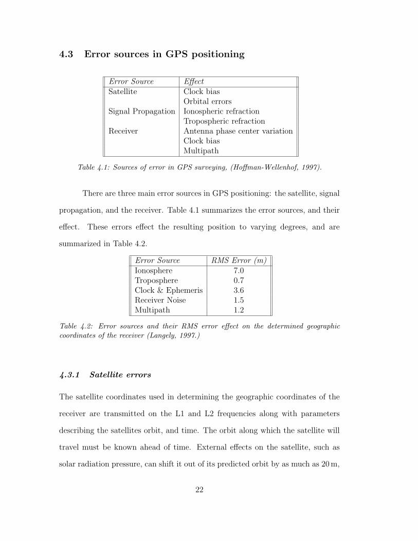
4.3 Error sources in GPS positioning

Error Source EffectSatellite Clock bias

Orbital errorsSignal Propagation Ionospheric refraction

Tropospheric refractionReceiver Antenna phase center variation

Clock biasMultipath

Table 4.1: Sources of error in GPS surveying, (Hoffman-Wellenhof, 1997).

There are three main error sources in GPS positioning: the satellite, signal

propagation, and the receiver. Table 4.1 summarizes the error sources, and their

effect. These errors effect the resulting position to varying degrees, and are

summarized in Table 4.2.

Error Source RMS Error (m)Ionosphere 7.0Troposphere 0.7Clock & Ephemeris 3.6Receiver Noise 1.5Multipath 1.2

Table 4.2: Error sources and their RMS error effect on the determined geographiccoordinates of the receiver (Langely, 1997.)

4.3.1 Satellite errors

The satellite coordinates used in determining the geographic coordinates of the

receiver are transmitted on the L1 and L2 frequencies along with parameters

describing the satellites orbit, and time. The orbit along which the satellite will

travel must be known ahead of time. External effects on the satellite, such as

solar radiation pressure, can shift it out of its predicted orbit by as much as 20 m,

22

with RMS (root-mean-square) errors of 5 m (Langely, 2000). Each GPS satellite

contains four atomic clocks to ensure that a stable timing system is maintained.

Although these clocks are extremely accurate, they can drift slightly resulting in

each satellites clock not being synchronized to one another. These errors in the

satellites orbital position and clocks can result in errors of 1–5 m in the resulting

geographic position.

A network of ground based GPS monitoring stations is operated by a

variety of research and military groups across the globe. The International GPS

Service (IGS) uses data collected by these sites to determine the true orbital path

and an estimate of the clock drift for each satellite. These are offered at no cost

to the GPS community on a variety of time scales. The most accurate are the

IGS final orbits, and are available for download over the internet two weeks after

the observation date.

Currently the IGS final orbits have an accuracy of 3–5 cm in the orbital

position of the satellite and an accuracy of 0.1–0.2 nanoseconds on the satellite

clock drift (Heroux et al., 2001). A substantial improvement in the accuracy of

the geographic receiver coordinates can be made by re-calculating the receiver

coordinates with the new satellite orbit and clock drift.

4.3.2 Propagation errors

GPS satellite signals experience various propagation delays as they travel through

the Earth’s atmosphere. These errors are mainly due to the ionosphere and to

the troposphere. The ionosphere is located from approximately 50 km–1000 km

above the surface, while the troposphere begins at the surface of the Earth and

extends to an altitude of 14 km. Satellites having low elevations with respect to

23

the horizon have higher ionospheric and tropospheric noise components because

of the greater amount of time spent travelling through these two layers. The

ionosphere is most active in a region extending approximately 20 on either side

of the magnetic equator, with high frequency scintillations experienced both in

this region, and over the poles (Janssen et al., 2002). Dual-frequency GPS re-

ceivers are able to remove this ionospheric effect by using a linear combination

of measurements on both frequencies (Janssen et al., 2002).

4.3.3 Receiver errors

The distance measured by the GPS receiver is the distance between the physical

phase centers of the GPS receiver and the GPS satellite. However the phase center

of the GPS receiver is unstable, and will change with the changing direction of

the satellite signal (Mader et al., 2002). Phase center variations can be accounted

for by modelling the response of the satellite antenna. The effect of phase center

variation is quite small and is not taken into account for our GPS prototypes.

A significant amount of receiver error can be generated through a process

known as multipath. Multipath is where GPS signals are reflected from surfaces,

such as the ground surface, or buildings, near the receiver and directed towards

the antenna. Because the signal has travelled along a longer path, it appears

that the satellite is further away than it actually is. Because ice is relatively

transparent to electro-magnetic waves, it is likely that multipath errors will not

be a concern for glacial GPS work.

GPS receivers contain inexpensive quartz oscillators which control the re-

ceiver clocks. By using a relatively inaccurate time keeping method there is an

inherent inaccuracy of the receiver clock resulting in positioning errors. Although

24

the unknown clock drift is taken into account and solved for in the iterative so-

lution method, it can still incorporate large errors into the resulting position.

4.4 GPS surveying considerations

4.4.1 Visible satellites

The GPS satellite constellation consists of six orbital planes inclined at 55 many

degrees. This configuration allows for maximum coverage over the continental

United States and Europe and ensures that at least 6 satellites are visible from

anywhere on the planet. In order to solve the positioning equations, four or

more GPS satellites must be visible to the GPS receiver. For higher latitudes,

the geometry of the satellite constellation can create difficulty in having enough

satellites in view for long periods of time, as the satellites appear low on the

horizon. This also makes the satellite orbits susceptible to being blocked by high

topography, which can be especially troublesome if the the GPS receivers are

situated in valleys.

Figure 4.3: GPS satellite orbits. The orbital planes of the satellites do not pass directlyover the poles.

25

4.4.2 Elevation cutoff mask

To prevent large errors from the ionospheric and tropospheric delays, satellites

below a certain cutoff elevation are usually excluded from being used in the

positioning solution. While this methodology can easily be applied for most GPS

surveys, closer to the poles it becomes a problem. At the poles, fewer satellites

will have a high elevation at any given time. This often results in fewer than four

satellites located above the cutoff elevation, and will require the incorporation of

satellites low in the horizon into the solution. For this thesis satellites at angle

of 15 with respect to the horizon are not incorporated into the solution.

26

5. GPS Prototype

A specialized GPS receiver system to track glacier motion has been designed

and built at the University of British Columbia, and has been operating at the

Trapridge Glacier research site since July 2002. This chapter will discuss the

design and operation of the GPS prototypes and review their main components.

Figure 5.1: The GPS receiver units, designed and built at the University of BritishColumbia, have been operating on Trapridge Glacier since July 2002.

From the beginning, the goal of the project was to develop a low-cost GPS

system which is suitable for harsh glacier environment and capable of tracking

glacier motion. The first prototypes were designed and built in the summer of

2002, and two units (displayed in Figure 5.1) were installed on Trapridge glacier.

In the summer of 2003, a new design was implemented that made use of dif-

27

ferent components, as well as a printed circuit board (PCB). A comparison of

the 2002 and 2003 prototypes showing their installation in Hoffman enclosures

is presented in Figure 5.2. It is clear that the incorporation of a PCB made the

devices easier to handle, install, and transport since there are significantly fewer

loose wires connecting the various components. The 2002 and 2003 prototypes

share the same basic design and operation; the only changes being in the various

electrical components selected. The final cost of the GPS prototypes is approx-

imately $500USD; this includes solar panels, Hoffman enclosures, and electrical

components.

5.1 Hardware

Figure 5.2: On the left is the 2002 GPS receiver prototype, on the right is the 2003 GPSreceiver prototype. The decision to use a printed circuit board made it much easier tooperate on the units in the field.

In Chapter 3 it is determined that all components used in the GPS pro-

totype must be able to operate at temperatures as low as –40C, and consume

very little power. The following sections will discuss the various components used

28

in the prototypes and outline some of their operating specifications. A detailed

schematic, PCB layout and part list for the 2003 prototype can be found in the

appendix.

5.1.1 GPS receivers and antennas

The GPS receivers handle all aspects of decoding and tracking the satellite sig-

nals. Low power Trimble Lassen SP GPS receivers were selected for the 2002

prototypes, while Garmin 15L GPS receivers were selected for the 2003 models.

Both of these GPS receivers record pseudo-range and carrier phase data on the

L1 frequency, and output the data through a serial data connection. The normal

operating power consumption of these receivers is less than 100 m A, and both

have operating specifications of –40C.

Skymaster II GPS antennas were selected for the 2002 unit, while Mighty

Mouse II antennas were used in 2003. These antennas both offered 28 dB of

signal gain, which serves to increase the signal–to–noise ratio. Both antennas

are encased in a sturdy environmental packaging and have a –40C operating

temperature specification. The Skymaster II antennas used 12 m A of current,

while the Might Mouse II draws only 5.0 m A.

5.1.2 Power supply

All aspects of the GPS prototypes are powered by 12V 6.5 Amp-hour lead acid

batteries. The batteries are continuously charged by 15 Watt solar panels. Power

from the solar panel is regulated to ensure that the batteries are not over charged

and to ensure that no large voltage spikes are sent to the battery. This battery

and solar panel configuration has been in use at Trapridge glacier for nearly a

29

decade and has proved reliable for use with data loggers. Since all components in

the GPS system are powered at 3.3V, two integrated-circuit voltage regulators

are used to step down the 12V battery to 3.3 V and supply power to the electronic

components. One power supply is used to provide power to the microcontroller,

while the other is used to provide power to the GPS and memory. This regulator

can be switched on and off by the microcontroller to turn on or off the peripherals.

5.1.3 Microprocessor and memory

The microprocessor is the brain of the device. It controls all aspects of the

device operation including timing, powering the peripherals, communication be-

tween the GPS and memory, and communication between the GPS device and

a personal computer. The environmental constraints of the systems required a

microprocessor with extremely low power consumption and a relatively low op-

erating temperature. Z-World Rabbit microprocessors were selected to operate

the 2002 GPS prototypes, while Texas Instruments MSP430 microprocessor was

selected for the 2003 GPS units and are recommended for future versions of the

GPS devices. Both of the Z-World and Texas Instruments microprocessors op-

erate with very little power and at –40C. The Texas Instruments MSP430 uses

only 250 µA of current when operating, and 1.6 µA in low power mode. An

external quartz oscillator was used to ensure that accurate timing was kept over

a wide range of temperature conditions.

Both microprocessors contain onboard flash memory, which is used to store

programs and data. The C computer language was used to write the software

which operates the devices. This enabled the software to be written and debugged

on a personal computer, and then transferred to the devices where it is written

30

into the flash memory. The use of C allowed various software components from

the first prototype to be re-used on the second prototype, and will allow the GPS

system to to be easily ported to different microprocessor architectures and future

systems.

Atmel data flash cards were used in both 2002 and 2003. In 2002, 4

megabyte cards were used and increased to 8 megabytes in 2003. These flash

memory card contain no moving parts, and can retain their memory when there

is no power; providing a robust system for storing the data. The cards also satisfy

the environmental operating specifications needed for work on the glacier.

5.1.4 Environmental enclosures and mounting hardware

With the exception of the GPS antennas, all components are mounted within

Hoffman environmental enclosures. These enclosures have proved reliable for

housing electronic components and have been used regularly for the Trapridge

Glacier field research.

To suspend the GPS receivers above the glacier surface, two inch diameter

steel pipes were drilled several meters into the glacier surface. Approximately

one meter is left outside of the ice surface to allow the Hoffman box and solar

panel to be mounted and to elevate it above the snow level. The solar panel is

mounted facing southeast towards a topographic low-point, ensuring the panels

obtain the maximum amount of solar energy.

5.2 GPS prototype operation

The basic operation of the GPS devices follows the flow chart in Figure 5.3. Once

powered up, the device tracks GPS satellites until it acquires enough satellites to

31

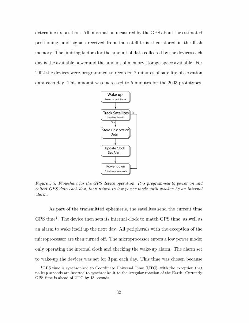
determine its position. All information measured by the GPS about the estimated

positioning, and signals received from the satellite is then stored in the flash

memory. The limiting factors for the amount of data collected by the devices each

day is the available power and the amount of memory storage space available. For

2002 the devices were programmed to recorded 2 minutes of satellite observation

data each day. This amount was increased to 5 minutes for the 2003 prototypes.

Figure 5.3: Flowchart for the GPS device operation. It is programmed to power on andcollect GPS data each day, then return to low power mode until awoken by an internalalarm.

As part of the transmitted ephemeris, the satellites send the current time

GPS time1. The device then sets its internal clock to match GPS time, as well as

an alarm to wake itself up the next day. All peripherals with the exception of the

microprocessor are then turned off. The microprocessor enters a low power mode;

only operating the internal clock and checking the wake-up alarm. The alarm set

to wake-up the devices was set for 3 pm each day. This time was chosen because

1GPS time is synchronized to Coordinate Universal Time (UTC), with the exception thatno leap seconds are inserted to synchronize it to the irregular rotation of the Earth. CurrentlyGPS time is ahead of UTC by 13 seconds

32

it would be at a warm time of the day and the battery would have acquired the

most of the power it would receive through solar energy that day. Once powered

up, the operation repeats itself. Should the device be unable to track satellites,

it sets the wake-up alarm based on its current clock and enters the low power

mode. It will repeat this cycle each day until a satellite lock is acquired.

Because each GPS device on the glacier synchronizes its internal clock to

match the GPS constellation time, they will each be powering up at the same time

every day and should track the same satellites over the same time period. This

methodology will potentially allow for differential post-processing to be applied

to the data collected by the GPS receivers located on the glacier.

33

6. Results

Two GPS devices, denoted 02GPS02 and 02GPS031, were deployed on Trapridge

glacier in July 2002 and left to operate throughout the winter. The two GPS

prototypes were separated by a distance of ∼150 meters along a line roughly

parallel with the direction of glacier flow; their positions on the glacier are shown

in Figure 6.1. In July 2003 these units were re-visited and their data was collected.

02GPS02

02GPS03

North

200m

Figure 6.1: Initial installation positions of 02GPS02 and 02GPS03 on TrapridgeGlacier. The two units were installed along a line roughly parallel to the directionof glacier flow.

6.1 Receiver status and data collected

Upon inspection in July 2003, both GPS receivers were found to be intact, having

survived the winter on Trapridge Glacier. Device 02GPS03 was operating per-

fectly when tested, while 02GPS02 had suffered from a battery failure sometime

during the winter.

1Convention in Trapridge Glacier research is to name sensors placed on the glacierYYXXXNN, where YY is the two digit year, XXX denotes the type of sensor, and NN isa two digit identifier.

34

6.1.1 02GPS02

Unit 02GPS02 collected a total of 62 days of data from July 21st, 2002, until

December 3rd, 2002, at which time it suffered a battery failure. In the 2003 field

season, it was discovered that the SunSaver solar regulators used to charge the

batteries required a large amount of power to preform their internal operations.

Should the battery voltage drop below a certain level, the regulator would no

longer operate and the battery would die completely. Upon replacing the battery,

unit 02GPS02 was found to be fully operational.

6.1.2 02GPS03

Unit 02GPS03 collected a total of 118 days of data from July 11th, 2002, until

January 5th, 2003. Unit 02GPS03 was found to have a fully charged battery and

to be fully operational when tested, yet it stopped collecting data on January,

5th 2003. Since approximately 1 megabyte of its 4 megabyte card was used, it is

likely that its failure was due to a software bug. Since no record is kept of when

the device wakes–up, it is unclear whether 02GPS03 was operational on any days

between January and July 2003, or if it remained dormant during this period.

6.1.3 Damage to the prototypes

Although both devices were operational upon inspection, 02GPS03 was found to

be tipped at a large angle, with its mounting pole being bent. This was most

likely due to strong winds experienced sometime during the winter. 02GPS02

was found to have sustained damage to its Hoffman enclosure, as shown in Figure

6.2, where a threaded screw hole was ripped from the sturdy Hoffman enclosure.

These damages illustrate the extreme conditions experienced by the receivers face

35

Figure 6.2: Damage sustained by 02GPS02 sometime during its over–wintering atTrapridge Glacier.

during the winter months on Trapridge Glacier. It is unclear whether the events

leading to the damage of the two devices is related to periods where they do not

collect data.

6.2 Unprocessed GPS positions

The GPS receivers determine their geographic coordinates automatically as they

track the satellites. This positioning is recorded in a data file along with the the

raw satellite information. The positions determined by 02GPS02 and 02GPS03

is presented in Figures 6.3 and 6.4 respectively. Since geographic coordinates are

determined by the GPS receivers once every 5 seconds, for 2 minutes each day that

they collected, the results in Figures 6.3 and 6.4 are the average position for each

day. Both receivers continued to operate throughout July 2003. Unfortunately,

an error resulted in the data collected by 02GPS02 to be lost, so only the results

from 02GPS03 show results from the summer of 2003.

Both 02GPS02 and 02GPS03 show large gaps in their recorded data, and

both failed to collect data during the month of November. Because there is

36

Aug02 Sep02 Oct02 Nov02 Dec02−2000

0

2000

Eas

ting

(m)

Aug02 Sep02 Oct02 Nov02 Dec02−5000

0

5000N

orth

ing

(m)

Aug02 Sep02 Oct02 Nov02 Dec02−2000

0

2000

4000

Ele

vatio

n (m

)

Figure 6.3: Unprocessed geographic coordinates from 02GPS02. Easting and Northingvalues have been subtracted from the mean.

no record of when the devices wake-up, it is unclear whether the devices awoke

during these periods, or if they remained dormant. Possible causes for these gaps

may be a failure to adequately acquire a lock on the satellite signals, insufficient

battery voltage, or a software malfunction.

The geographic locations determined by both GPS devices show a large

amount of scatter. From July–August 02GPS02 appeared to collect data with an

expected amount of scatter, on the order of ±10 m. 02GPS02 then remains dor-

mant for 2.5 months, during which time it collects no data. The device then be-

gins to collect data in October. Positions determined by 02GPS02 from October–

December, exhibits an extreme, showing variations of over 1000 m from the mean

(Figure 6.3). The poor quality of data collected by 02GPS02 in the later part of

the year after a period of being dormant may be caused by damage to the GPS

antenna, damage to the GPS receiver, or a low battery. Because there is no data

37

Oct02 Jan03 Apr03 Jul03−10

0

10

20

Eas

ting

(m)

Oct02 Jan03 Apr03 Jul03−20

0

20N

orth

ing

(m)

Oct02 Jan03 Apr03 Jul032340

2360

2380

2400

Ele

vatio

n (m

)

Figure 6.4: Unprocessed geographic coordinates from 02GPS02. Easting and Northingvalues have been subtracted from the mean.

from the summer of 2003 for this device, it is unclear whether this GPS device

continued to collect data with a higher than expected amount of error. Positions

determined by 02GPS03 from July–January 2003 exhibit scatter on the horizontal

positions on the order of ±10 m. Data was collected by 02GPS03 in July of 2003,

and exhibits similar amounts of scatter. A definite movement trend can be seen

in the horizontal coordinates for 02GPS03. The Easting coordinate increases on

the order of 10–15 m, and the horizontal component shows very little movement

trend. This matches the general movement trends observed on Trapridge Glacier,

as discussed in Chapter 3.

38

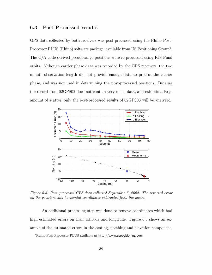
6.3 Post-Processed results

GPS data collected by both receivers was post-processed using the Rhino Post-

Processor PLUS (Rhino) software package, available from US Positioning Group2.

The C/A code derived pseudorange positions were re-processed using IGS Final

orbits. Although carrier phase data was recorded by the GPS receivers, the two

minute observation length did not provide enough data to process the carrier

phase, and was not used in determining the post-processed positions. Because

the record from 02GPS02 does not contain very much data, and exhibits a large

amount of scatter, only the post-processed results of 02GPS03 will be analyzed.

0 10 20 30 40 50 60 70 80 900

5

10

15

20

seconds

Est

imat

ed E

rror

(m

) σ Northingσ Eastingσ Elevation

−12 −10 −8 −6 −4 −2 0 2 4−10

0

10

20

30

Nor

thin

g (m

)

Easting (m)

MeanMean, σ < c

Figure 6.5: Post–processed GPS data collected September 5, 2002. The reported erroron the position, and horizontal coordinates subtracted from the mean.

An additional processing step was done to remove coordinates which had

high estimated errors on their latitude and longitude. Figure 6.5 shows an ex-

ample of the estimated errors in the easting, northing and elevation component,

2Rhino Post-Processor PLUS available at http://www.uspositioning.com

39

along with the horizontal coordinates for data collected on September 5, 2003

using 02GPS03. Coordinates exhibiting high error estimates were not included

in the calculation of the average daily position. This essentially removes the data

points that were collected right when the GPS obtained a satellite lock. Figure

6.5 shows that using points with error estimates of less than 1.0m Easting and

1.6m Northing, obtains an average position which differs by 2.5m Easting, and

7.0m Northing is obtained than by using all the positions determined by the GPS

that day.

Oct02 Jan03 Apr03 Jul03−10

0

10

20

Eas

ting

(m)

Oct02 Jan03 Apr03 Jul03−20

−10

0

10

20

Nor

thin

g (m

)

Oct02 Jan03 Apr03 Jul032350

2400

2450

Ele

vatio

n (m

)

Figure 6.6: Post-processed geographic coordinates from 02GPS03. Easting and Nor-thing values have been subtracted from the mean.

The results of post-processed data, shown in Figure 6.6, show some im-

provement in the derived easting coordinate for 02GPS03, and negligible improve-

ment for the northing and elevation. It is likely that not long enough observation

periods were collected each day by the GPS devices for post-processing with

IGS final orbital ephemeris to result in significant improvements of the resulting

40

geographic positions.

Although the Rhino software is not explicit in how it produces it’s error

estimate, it is likely a combination of the satellite geometry and the amount of

scatter present in the data. It appears under-estimate the amount of error present

in the data. For most days of GPS observations, errors determined by Rhino for

the easting and northing components usually reach as low as ∼0.5m. By looking

at the resultant averages in Figure 6.6, it is clear that the overall positioning

error is on the order of ±5m in the Easting, and ±10m for the Northing.

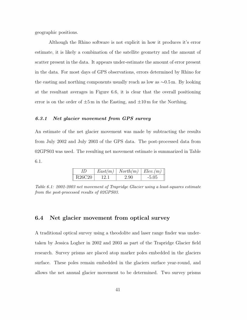
6.3.1 Net glacier movement from GPS survey

An estimate of the net glacier movement was made by subtracting the results

from July 2002 and July 2003 of the GPS data. The post-processed data from

02GPS03 was used. The resulting net movement estimate is summarized in Table

6.1.

ID East(m) North(m) Elev.(m)R26C20 12.1 2.90 -5.05

Table 6.1: 2002-2003 net movement of Trapridge Glacier using a least-squares estimatefrom the post-processed results of 02GPS03.

6.4 Net glacier movement from optical survey

A traditional optical survey using a theodolite and laser range finder was under-

taken by Jessica Logher in 2002 and 2003 as part of the Trapridge Glacier field

research. Survey prisms are placed atop marker poles embedded in the glaciers

surface. These poles remain embedded in the glaciers surface year-round, and

allows the net annual glacier movement to be determined. Two survey prisms

41

close to the GPS sites were selected. By subtracting their coordinates from 2003

to 2002 the net glacial movement for the year (Table 6.2).

ID East(m) North(m) Elev.(m)R26C20 11.74 1.89 -3.62R32C20 12.11 2.10 -1.28

Table 6.2: 2002-2003 displacements as measured by the optical survey.

Horizontal displacements at both survey targets are similar, and show

movement on the order of 12 meters East, and 2 meters North. The discrepancy

in the elevations taken at the two points may be due to melting experienced by

the flow poles causing one of them to sink further into the ice than the other, and

deformation of the survey poles by wind during the winder. Although the survey

poles report an elevation drop on the order of meters, the elevation changes are

more likely on the order of 0.1–0.5m for the two survey positions.

6.5 Annual velocity model for Trapridge Glacier

A least-squares method was used to fit two linear functions to the post-processed

data of Figure 6.6. The results of this fitting are shown in Figure 6.7. The

two blue lines in Figure 6.7 are interpolations between the least-squares derived

estimate for the first six months of the year, and the data from July 2003. The

two lines correspond to upper and lower limits for the velocity during the last 6

months of the year.

The velocity for the first half of the year is found to be 17.6 m a−1. To

determine how sensitive this velocity estimate was the first and last data points

in this period, the least squares estimate was preformed removing the first three

data points, and again removing the last three data points. It was found with

42

Jul02 Oct02 Jan03 Apr03 Jul03 Oct03−10

0

10

Eas

ting

(m)

Figure 6.7: Least squares derived velocity model for Trapridge glacier using two linearvelocity trends.

these points removed varied with ±1.1 m a−1.

The velocity for the January–July 2003 is estimated by an upper and

lower bound to the velocity during this period. The lower bound is taken to

be 0.0 m a−1, and the upper bound is found to be 6.9 m a−1. The occurrence of

a spring/summer velocity mode and a winter mode has been observed on other

glaciers (Willis et al. (2003), Hubbard et al. (1998)).

43

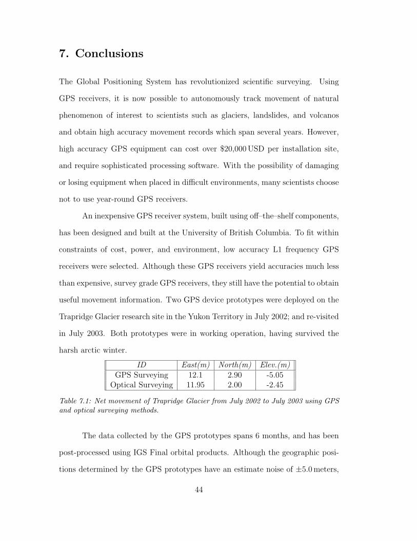
7. Conclusions

The Global Positioning System has revolutionized scientific surveying. Using

GPS receivers, it is now possible to autonomously track movement of natural

phenomenon of interest to scientists such as glaciers, landslides, and volcanos

and obtain high accuracy movement records which span several years. However,

high accuracy GPS equipment can cost over $20,000USD per installation site,

and require sophisticated processing software. With the possibility of damaging

or losing equipment when placed in difficult environments, many scientists choose

not to use year-round GPS receivers.

An inexpensive GPS receiver system, built using off–the–shelf components,

has been designed and built at the University of British Columbia. To fit within

constraints of cost, power, and environment, low accuracy L1 frequency GPS

receivers were selected. Although these GPS receivers yield accuracies much less

than expensive, survey grade GPS receivers, they still have the potential to obtain

useful movement information. Two GPS device prototypes were deployed on the

Trapridge Glacier research site in the Yukon Territory in July 2002; and re-visited

in July 2003. Both prototypes were in working operation, having survived the

harsh arctic winter.

ID East(m) North(m) Elev.(m)GPS Surveying 12.1 2.90 -5.05

Optical Surveying 11.95 2.00 -2.45

Table 7.1: Net movement of Trapridge Glacier from July 2002 to July 2003 using GPSand optical surveying methods.

The data collected by the GPS prototypes spans 6 months, and has been

post-processed using IGS Final orbital products. Although the geographic posi-

tions determined by the GPS prototypes have an estimate noise of ±5.0meters,

44

averaging was used to estimate the net annual movement of Trapridge Glacier.

The result obtained through least squares is in agreement with the amount of net

movement obtained through traditional optical surveying, and is summarized in

Table 7.1.

A linear two-velocity model was determined from the post-processed GPS

results using a least-squares method. This velocity model suggests that Trapridge

Glacier experiences summer/spring velocities of 17.6 m a−1, and winter/fall ve-

locities of between 0.0–6.9 m a−1. Studies of Trapridge Glacier have shown that

it has experienced net annual movement on the order of 30 m a−1 (Kavanaugh,

2000). Results of this study suggest that Trapridge Glacier is experiencing annual

movement rates of approximately 12 m a−1.

This study demonstrates the feasibility for low-cost GPS receivers to track

glacier motion in a harsh arctic setting. This system, which can easily be fabri-

cated by scientists, has demonstrated the potential for low–cost GPS receivers of

this nature to obtain useful scientific information.

45

8. Recommendations for Further Work

The results presented in this thesis demonstrate the ability of low cost GPS

systems to operate in harsh glaciated environments. Experience gained through

operating the devices in the field from both the 2002 and 2003 field seasons

should be incorporated into future devices. Experience from the 2003 field season

illuminated several shortcomings of the current design. The following sections are

possible improvements which can be made to both the design of the GPS system

hardware, and to the survey design and data processing.

8.1 GPS survey improvements and recommendations

The 2002 GPS devices analyzed in this these each measured two minutes of GPS

data per day. This short observation length did not yield adequate data for post-

processing and limited the post-processing to C/A code derived pseudo-ranges,

and it is unlikely that the increase to five minutes observation lengths in the

2003 models will improve this result. Significant improvements in accuracy may

be obtained by using differential processing techniques on the L1 carrier phase.

Differential post-processing require much longer observation periods in order to

track changes in the carrier phase. Hoffman-Wellenhoff et al. (1995) recommend,

that at a minimum, 20 minutes of observation be used for differential processing,

plus additional time for large receiver/base station separation distances. The

observation length for the GPS prototypes should be determined through field

testing, as it will depend on both the GPS receiver/antenna, and the processing

software involved. The additional power and memory requirements needed to

accommodate the longer observation period need to be addressed to ensure that

46

it is realizable within the constraints of the system.

Differential processing will also require a stationary base station. This base

station should be located on the lateral moraine of Trapridge Glacier, such that it

is visible from the LN survey site to allow it’s location to be accurately surveyed.

Multiple base stations should be deployed to guard against the possibility of a

base station failing. Additional base stations could also be incorporated into the

differential post-processing, such as done in Janssen et al. (2002).

Currently, the GPS receivers power on at 3 pm each day. Although it may

be possible to determine a wake-up time each day to ensure that an optimal

satellite constellation geometry is obtained, it is not recommended to do so.

Changes to the wake-up time could cause all receivers on the glacier lose their

time synchronization, or cause the device to wake-up at times when it is colder

and darker.

8.1.1 Processing software

Complex software packages are required to post-process GPS data. Several pro-

fessional processing packages are available, but at a cost of several thousand dol-

lars. Two free processing packages available are GAMIT/GLOBK1 and GIPSY-

OASIS2. The GAMIT/GLOBAK software was tested on the 2002 data, but I was

unable to get the software to work. Further investigation needs to be done to ex-

plore the potential of these software packages to post-process the GPS data. The

U.S. Positioning Rhino Post Processing software used to post-process the 2002

data, and is available for around $300USD. In addition to the post-processing

software, various pieces of software were needed to convert the data into the

1GAMIT: http://www-gpsg.mit.edu/∼simon/gtgk/2GIPSY-OASIS: http://gipsy.jpl.nasa.gov/

47

RINEX3 format

8.2 Hardware improvements and recommendations

Various shortcomings in the design and layout of the electronic components sur-

faced when the GPS devices were deployed and operated in the field.

8.2.1 Memory storage and transfer

The Garmin GPS 15L receivers currently output approximately 0.3 kilobytes-

per-second. With this data rate, collecting twenty minutes of data per day for

an entire year would require approximately 1.3 gigabytes of storage, although

some of the data output by the GPS can be neglected to reduce this memory

requirement. The current GPS device uses 8 megabyte flash memory, which is

clearly not enough to handle the large amount of data. To further reduce the

storage requirement it may be possible to reduce the sampling frequency. The

2002 GPS prototypes used a sample frequency of 0.2Hz (1 observation every 5

seconds) which allowed them to maximize their 4-megabyte flash memory. The

effects of reducing the sample frequency may create difficulties when preforming

the differential post-processing, and should be investigated further.

Obtaining the GPS data is currently handled by connecting the GPS to a

personal computer via the serial port. Raw binary information is sent over the

serial connection at a speed of 9600 kbps (kilo-bits per second). At this rate, an 8

megabyte memory card would take just under 2 hours to transfer. Furthermore,

there is no error checking on the communication so there is a large possibility

for transfer data errors or missing data. This method of transferring data also

3The Receiver Independent Exchange Format (RINEX) is a format for storing the GPSobservations for processing.

48

requires using a laptop on the glacier surface, which limits the weather conditions

and mobility of the operator in gathering the data.

A new memory storage system needs to be developed. To transfer this

large amount of data to a computer, it is necessary to use a specialized card

reader. To be compatible with these card readers, the data must be stored in

using either the FAT–16, or FAT–32 filesystems4. Compact flash or Multimedia

(MMC) cards with sizes of 128 or 256 megabytes should be selected for the new

memory system. This will allow cards to be swaped from the GPS devices and

transferred at a later time.

8.2.2 PCB design and component selection

Thru-hole components should be selected over surface mount components when

they are available. This will make it easier to replace components in the field,

and will remove dependency on specialized soldering equipment and expertise

required to solder surface mount components. However, some parts, such as

the Texas Instruments microcontroller are not available in thru-hole packaging.

Two options for the microcontroller are to design and build a header board, or

purchase one from a vendor5.

Header pins can be incorporated into the circuit board for a very small

cost. These pins will allow multimeters and other testing equipment to be easily

attached to the various components on the circuit board, as the current design

makes this nearly impossible because of the small component size. Experience

has shown that in some instances, the probe of the multimeter can connect two

pins together, causing a short circuit, and results in damage to the device. Header

4File Allocation Table (FAT) formats are format for storing data developed by Microsoft.5MSP430 header boards are available from Olimex, http://www.olimex.com

49

pins will also enable new features to be added and tested to the devices without

re-designing the circuit board.

Incorporating protection diodes into the design of the power supply will

prevent the board from sustaining damaged in the event that the battery is

attached with the wrong polarity. It was also found that the current voltage

regulators did not provide adequate protection from voltage spikes caused by

static-electric discharge when operator comes in contact with the device. The

operator should ensure adequate grounding when working on the device, and a

proper grounding system should be purchased for future development.

8.2.3 PCB layout and mounting

The current PCB layout positions the GPS receiver on the underside of the circuit

board. This creates a serious difficulty when attaching the GPS antenna, and

required that the back-plate be removed when attaching the antenna. Future

designs must ensure that the layout allows convenient access when attaching

the antenna, battery connectors, or memory card when the device is inside the

Hoffman enclosure with the battery.

The GPS device is mounted with machine screws to a steel back-plate

within the Hoffman enclosure, and is elevated using plastic stand-offs. To remove

the device, it is first required to remove the back-plate to access the mounting

screws. This process can take considerable time and can lead to damage of

the device. Also, in the event that the GPS receiver itself was in-operable, the

entire GPS device had to be removed by the same procedure. Future designs

should allow for quick removal of the GPS receiver and the GPS board which will

allow for quicker maintenance and troubleshooting, and will reduce the risk of

50

accidental damage to the device when removing it from the Hoffman enclosure.

8.2.4 Measurement of battery voltage and temperature

The MSP430 chipset contains several analogue–to–digital (A/D) converters which

can be used to measure the voltage of the 12V battery. Software logic could

then be implemented to prevent the system from running should the battery

voltage fall below a certain point. Data loggers on Trapridge Glacier are currently

programmed to stop execution should the battery voltage drop below 11.8V. A

suitable level of voltage cutoff should be determined for the GPS devices based

on the energy requirements of the solar regulator, and the amount of current the

GPS device will consume when operating. Protection diodes and surge protection

will need to be incorporated to prevent damaging the microcontroller in the event

of incorrect battery polarity or static shock. The MSP430 also has the ability to

measure temperature using the A/D converter, by incorporation of a thermistor

circuit. This temperature could be monitored, and could suspend operation of

the device should the temperature drop below the operating specifications of the

components.

8.3 Software improvements and recommendations

The compiler used for development thus far has been IAR Systems Embedded

Workbench. A limited– use compiler was provided with the MSP430 development

kits purchased from Texas Instruments, and was limited in the size of executables

it could generated. To overcome this limit, a 30-day demo of the full version of

IAR Embedded Workbench was used to finish development of the software. This

30-day limit almost proved disastrous when development of the software needed

51

to be complete at the Trapridge Glacier field site. However, a free compiler for

the Texas Instruments MSP430 product line, MSPGCC6 has been under develop-

ment. This compiler has advanced to the point that is is now a viable alternative

to IAR Systems Embedded Workbench. Future development should be done with

the MSPGCC compiler.

Currently the GPS devices do not store a record of when they power-up. A

log file should be kept which tracks the date, time, battery voltage, temperature

and the GPS satellite tracking status each time the device powers on. There

are several periods during 2002-2003 in which no GPS data was collected by the

devices (Figure 6.4). Currently no account can be made for why the device failed

to collect data during these periods.

6MSPGCC is an open source port of the GCC compiler, http://mspgcc.sourceforge.net/

52

A. Visible Satellites at Trapridge Glacier

To understand the distribution of visible GPS satellites above Trapridge Glacier,

several skyplots have been generated. The following skyplots show where GPS

satellites will be visible in the sky, and show traces of their movement.

A.1 Trapridge Glacier

Figures A.1 and A.2 show skyplots over Trapridge Glacier on July 16, 2003.

Figure A.1 shows the satellite constellation for a two hour period centered around

the observations made by the GPS prototypes on that day at 22:00. An elevation

cutoff mask of 10 is used, so satellites below this mask are not plotted. The

satellites in the northern portion of the sky have low elevations, and are likely

to not be used in the positioning solutions. At the time of observation, the

GPS prototypes would have had 8 visible satellites; enough for a positional fix.

However, satellites 4, 7, 11, 30 are low in the sky at this point in time, and may

bring additional errors into the resulting position.

Figure A.2 shows an 11 hour skyplot for Trapridge Glacier on July 16, 2003.

It is clear to see that there is a large empty hole in the northern portion of the plot

where no satellites will ever be visible due to the geometry of the satellites orbits.

The very nature of the satellite orbit geometry favors East–West coordinates over

the North–South coordinates as the satellite geometry provides more constraints

on the East–West coordinates.

53

A.2 North pole and Equator

For comparison, skyplots for the north pole, and the equator are displayed in

Figures A.4 and A.3. No satellites are visible above 45 at the north pole, while

at the equator, all portions of the sky are covered by GPS satellites.

54

TRAPRIDGE Lat: 61.2200 Lon: -140.3400 Ell Ht: 2400.0 (m)

GPS Time: Start 2003/07/16 21:00:00 Stop 2003/07/16 23:00:00

21h

21h

21h

21h

21h

21h

21h

21h

22h

22h

22h

22h

22h

22h

22h

N

S

W E

45û

135û 225û

315û

1

4

5

7

11

13

14

16

20

24

25

30

0û 30û 60û 90û 10û

Figure A.1: Satellite coverage at Trapridge Glacier for July 16, 2003 for 2 hours duringthe time the GPS data observations were collected.

55

TRAPRIDGE Lat: 61.2200 Lon: -140.3400 Ell Ht: 2400.0 (m)

GPS Time: Start 2003/07/16 12:00:00 Stop 2003/07/16 23:00:00

12h

12h

12h

12h

12h

12h

12h

12h

12h

12h

13h

13h

13h

13h

13h

13h

13h

13h

13h

13h

14h

14h

14h

14h

14h

14h

14h

14h

14h

15h

15h

15h

15h

15h

15h

15h

15h

15h

15h

15h

15h

15h

16h

16h

16h

16h

16h

16h

16h

16h

16h

16h

16h

16h

17h

17h

17h

17h

17h

17h

17h

18h

18h

18h

18h

18h

18h

18h

18h

18h

19h

19h

19h

19h

19h

19h

19h

19h

19h

20h

20h

20h

20h

20h

20h

21h

21h

21h

21h

21h

21h

21h

21h

22h

22h

22h

22h

22h

22h

22h

N

S

W E

45û

135û 225û

315û

1

2

3

4

5

6

7

8 9

10

11

13

14

15

16

17

18

20 21

23

24

25

26 27

28

29

30

31

0û 30û 60û 90û 10û

Figure A.2: Satellite coverage at Trapridge Glacier for July 16, 2003 for 11 hours.This shows the general spatial extent that Trapridge Glacier will obtain from the GPSsatellite geometry.

56

Equator Lat: 0.0000 Lon: 0.0000 Ell Ht: 1.0 (m)

GPS Time: Start 2003/07/16 12:00:00 Stop 2003/07/16 23:00:00

12h

12h 12h

12h

12h

12h

12h

12h

13h

13h

13h

13h

13h

13h

13h

13h

13h

14h

14h

14h

14h

14h

14h

14h

15h

15h

15h

15h

15h

15h

15h

15h

16h

16h

16h

16h

16h

16h

16h

17h

17h

17h

17h

17h

17h

17h

17h 17h

18h

18h

18h

18h 18h

18h

18h

18h

18h

19h

19h

19h

19h 19h

19h

19h

19h

19h

19h

20h

20h

20h

20h 20h

20h

20h

20h

20h

20h

21h

21h

21h

21h

21h

21h

21h

21h

21h

21h

21h

22h

22h

22h

22h

22h

22h 22h

22h

22h

22h

N

S

W E

45û

135û 225û

315û

4

5

6

7

8

9

10

11

13

14

15

17

18

20

21

23

24

26

27 28

29

30

0û 30û 60û 90û 10û

Figure A.3: Satellite coverage at the Equator.

57

North_Pole Lat: 90.0000 Lon: 0.0000 Ell Ht: 1.0 (m)

GPS Time: Start 2003/07/16 12:00:00 Stop 2003/07/16 23:00:00

12h

12h

12h

12h

12h

12h

12h

12h 12h

13h

13h

13h

13h

13h

13h

13h

13h

13h

13h

14h

14h

14h

14h

14h 14h

14h

14h

14h

14h

14h

15h

15h

15h 15h

15h

15h

15h

15h

15h

15h

15h

15h

16h

16h

16h

16h

16h

16h

16h

16h

16h

16h

16h

16h

16h

17h

17h

17h

17h

17h

17h

17h

17h

17h

17h

18h

18h

18h

18h

18h

18h

18h

18h

18h

19h

19h

19h

19h

19h

19h

19h

20h

20h

20h

20h

20h

20h

20h

21h

21h

21h

21h

21h

21h

21h

21h

21h

22h

22h

22h

22h

22h

22h

22h

22h

22h

N

S

W E

45û

135û 225û

315û

1

2 3

4

5

6

7

8

9

10

11 13

14

15

16

17

18

20

21

23

24

25

26

27

28

29

30

31

0û 30û 60û 90û 10û

Figure A.4: Satellite coverage over the north pole.

58

B. Linearized GPS Solution

Determination of the unknown geographic coordinates of the receiver from the

observations made by the receivers antenna requires solving a non-linear system

of equations. Recall from chapter 4 the mathematical model of the pseudo-range

measured for each satellite by the GPS receiver:

P = ρ + cδt + Ttrop + Tion + Trel + ε (B.1)

Where P is the pseudo-range, ρ is the exact geometric distance, c is the speed

of light in a vacuum, δt is the unknown clock bias, Ttrop is the signal path delay

due to troposphere, Tion is the signal path delay due to the ionosphere, Trel is the

signal delay due to relativistic errors due to the high satellite velocity and ε is an

estimate of the noise. By neglecting the tropospheric, ionospheric, and receiver

errors equation B.1 becomes

P = ρ + cδt (B.2)

The geometric distance between the jth satellite and the receiver is given by

ρj =√

(Xj −X)2 + (Y j − Y )2 + (Zj − Z)2 (B.3)

All that remains is to solve the equation for the the unknown receiver coor-

dinates, (X,Y, Z). A Taylor series expansion is used to expand Equation B.2

about estimates of the geographic coordinates of the receiver, (X0, Y0, Z)), and

the higher order terms are dropped. Perturbations (∆X, ∆Y, ∆Z) in Equation

B.4 are solved at each iteration, until they become negligible in size.

59

P ik ≈ P0 +

∂P ik

∂X0

|(X0,Y0,Z0)∆X +∂P i

k

∂Y0

|(X0,Y0,Z0)∆Y +∂P i

k

∂Z0

|(X0,Y0,Z0)∆Z + cδt0 (B.4)

Where P0 is the pseudo-range estimated from the approximate receiver coordi-

nates. Substituting the derivative of Equation B.2 and simplifying results in a

linear equation of the perturbations.

P ik ≈ P0 +

(X0 −Xj)∆X + (Y0 − Y j)∆Y + (Z0 − Zj)∆Z√(X0 −Xj)2 + (Y0 − Y j)2 + (Z0 − Zj)2

+ cδt0 (B.5)

Letting ρ0 be the geometric distance from the estimated receiver position to the

satellite, and defining ∆P ik as

∆P ik = P i

k − P0 (B.6)

results in the system of linear equations which are solved

∆P ik =

(X0 −Xj)

ρ0

∆X +(Y0 − Y j)

ρ0

∆X +(Z0 − Zj)

ρ0

∆X + cδt0 (B.7)

Assuming that 4 satellites are being tracked, the system has four unknowns: the

3 receiver coordinates, and the clock bias. The resulting matrix is

∆P1

∆P2

∆P3

∆P4

=

(X0−X1)ρ1

(Y0−Y 1)ρ1

(Z0−Z1)ρ1

1

(X0−X2)ρ2

(Y0−Y 2)ρ2

(Z0−Z2)ρ2

1

(X0−X3)ρ3

(Y0−Y 3)ρ3

(Z0−Z3)ρ3

1

(X0−X4)ρ4

(Y0−Y 4)ρ4

(Z0−Z4)ρ4

1

∆X

∆X

∆X

cδt

(B.8)

Which is a matrix system of equations A~x = ~b. This system can be solved using

a least squares, or generalized inverse operator:

The new estimate of the receiver position is updated after each iteration,

60

(Xn, Yn, Zn) = (Xn−1, Yn−1, Zn−1) + (∆X, ∆Y, ∆Z) (B.9)

The process is iterated until convergence, when

‖(∆X, ∆Y, ∆Z, δt)‖ ≈ 0 (B.10)

B.1 ECEF coordinate system

The coordinate system used for this solution is the Earth Centered Earth Fixed

(ECEF) coordinate system. The ECEF coordinate system places the center of

mass of the earth’s reference ellipsoid at (0, 0, 0). A coordinate transformation

can be applied to convert the (X, Y, Z) ECEF coordinates obtained in the

solution to WGS-84 Latitude/Longitude, or UTM coordinates.

61

C. Trapridge Coordinate Transformation

Surveying has taken place on Trapridge Glacier for more than three decades.

To place the positions surveyed at Trapridge Glacier to a map system, the lati-

tude and longitude of the Trapridge Glacier survey site were determined by Sam

Collins. This was accomplished by determining the longitude and latitude of the

survey location by monitoring the Sun and the Moon, and was likely based on

the NAD–27 mapping datum, which is standard for government maps of Canada.

With the advent of GPS, Trapridge Glacier can now be accurately tied to the

commonly used map datum, WGS–84. A transformation can now be applied

to convert the historic Trapridge survey data to the WGS–84 datum. Once in

this established map datum, further transformations can be applied to convert

Trapridge survey coordinates to any mapping system.

C.1 Method

Several locations exist on or near Trapridge in which both the GPS determined

coordinates, and the relative Trapridge coordinates are known. Trapridge coor-

dinates exist in a pseudo-UTM form of Easting, Northing, and Elevation.

In 2003 a Garmin eTrex Vista handheld GPS receiver was used to obtain WGS–

84 coordinates of several points around Trapridge Glacier, Figure C.1 shows the

comparison of the GPS points to the Trapridge points. Clearly, there is a simple

shift to translate one set of coordinates to the other.

62

Figure C.1: Trapridge Survey Positions plotted along side the same locations measuredwith a GPS unit using the WGS–84 map datum.

C.2 Results

By taking the average Easting, Northing and Elevation difference between the

WGS–84 coordinates and the Trapridge UTM coordinates, a transformation can

be defined that will place traditional Trapridge survey coordinates into the WGS–

84 datum. From this point, further coordinate transformations can take place to

place results of the Trapridge Glacier survey in any mapping system. Table C.3

shows the difference between Trapridge coordinates, and GPS derived WGS–84

coordinates. The last row displaying the average difference, and provides the

transformation Equation C.1.

(x, y, z)WGS84 = (x, y, z)TRAP + (96.091 m,−154.721 m,−11.460 m) (C.1)

Where (x, y, z)TRAP are the Easting, Northing, and Elevation in Trapridge pseudo-

UTM coordinates, and (x, y, z)WGS84 are the Easting, Northing, and Elevation

in WGS–84.

63

ID Easting(m) Northing(m) Elevation(m)02GPS02 535618.885 6787741.735 2373.10002GPS03 535762.038 6787776.420 2355.000

LN 536216.223 6788600.271 2347.380TN 534874.626 6788135.605 2543.952HK 538361.800 6787497.165 2358.289

Table C.1: Trapridge pseudo–UTM coordinates obtained through traditional surveytechniques.

ID Easting(m) Northing(m) Elevation(m)02GPS02 535533.945 6787891.345 2388.70002GPS03 535673.233 6787926.177 2371.000

LN 536104.000 6788760.000 2355.000TN 534791.940 6788289.281 2554.000HK 538250.000 6787658.000 2367.000

Table C.2: Trapridge WGS–84 Coordinates obtained through GPS measurements in2003.

ID Easting(m) Northing(m) Elevation(m)02GPS02 84.9400 -149.610 -14.90002GPS03 88.8050 -149.757 -16.000

LN 112.223 -159.729 -7.620TN 82.686 -153.676 -10.050HK 111.800 -160.835 -8.710AVG 96.091 -154.721 -11.460

Table C.3: Difference between GPS WGS–84 coordinates and Trapridge coordinates,and average difference.

C.3 Applicability of Results

The above results use only a simple average to determine a transformation be-

tween WGS–84 and Trapridge–UTM coordinates. Details such as the curvature

of the earth, and rotations between the two coordinate systems have not been

taken into account. Due to the relative low accuracy of the GPS derived posi-

tions of ∼9 meters horizontal, and ∼18 meters vertical, a more general coordinate

transformation would yield little new information. However, the transformation

derived above is applicable only for the immediate region of Trapridge glacier

64

and should not be applied for distances of more than a few kilometers away from

the glacier.

65

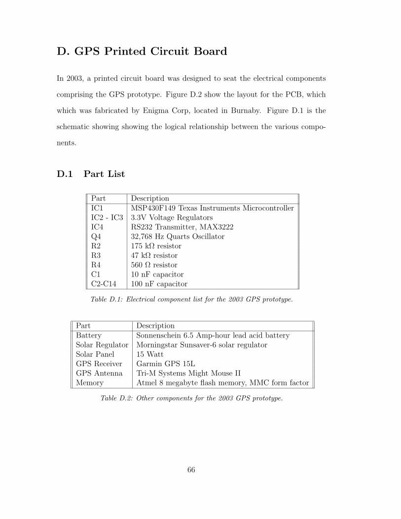
D. GPS Printed Circuit Board

In 2003, a printed circuit board was designed to seat the electrical components

comprising the GPS prototype. Figure D.2 show the layout for the PCB, which

which was fabricated by Enigma Corp, located in Burnaby. Figure D.1 is the

schematic showing showing the logical relationship between the various compo-

nents.

D.1 Part List

Part DescriptionIC1 MSP430F149 Texas Instruments MicrocontrollerIC2 - IC3 3.3V Voltage RegulatorsIC4 RS232 Transmitter, MAX3222Q4 32,768 Hz Quarts OscillatorR2 175 kΩ resistorR3 47 kΩ resistorR4 560 Ω resistorC1 10 nF capacitorC2-C14 100 nF capacitor

Table D.1: Electrical component list for the 2003 GPS prototype.

Part DescriptionBattery Sonnenschein 6.5 Amp-hour lead acid batterySolar Regulator Morningstar Sunsaver-6 solar regulatorSolar Panel 15 WattGPS Receiver Garmin GPS 15LGPS Antenna Tri-M Systems Might Mouse IIMemory Atmel 8 megabyte flash memory, MMC form factor

Table D.2: Other components for the 2003 GPS prototype.

66

Figure D.1: Schematic for the 2003 GPS prototypes.

67

Figure D.2: Printed circuit board design for the 2003 GPS prototypes.

68

References

Blake, E. W., 1992. The Deforming bed Beneath a Surge-Type Glacier: Mea-

surements of Mechanical and Electrical Properties. (Ph.D. thesis, University

of British Columbia).

Clarke, G. and Blake, E. W. 2002. Geometric and thermal evolution of a

surge-type glacier in its quiescent state: Trapridge Glacier, Yukon Territory,

Canada, 1969-89. J . Glaciol. 37(125), 158–169.

Eiken, T., Hagen, J.O. and Melvold, K. 1997. Kinematic GPS survey of

geometry changes on Svalbard glaciers. Ann. of Glaciol., 24, 157–163.

Flowers, G. E. 2000. A Multicomponent Coupled Model of Glacier Hydrol-

ogy. (Ph.D. thesis, University of British Columbia).

Frezzotti, M., Capra, A. and Vittuari, L. 1998. Comparison between Glacier

Ice Velocities Inferred from GPS and Sequential Satellite Images. Ann. of

Glaciol., 27, 54–60.

Harrison, W. D., Raymond, C. F., Sturm, M., Echelmeyer, K. and Humphrey

N. F. 1989. First Results from Automated Motion and Stream Mea-

surements from Fels and Black Rapids Glaciers, Alaska. (Abstract).

Ann. of Glaciol., 12, 203.

69

Heroux, P. and Kouba J. 2001. GPS Precise Point Positioning Using IGS

Orbit Products. Phys. Chem. Earth., 26, 573–278.

Hofmann-Wellenhof, B., Lichtenegger, H. and Collins J. 1997. GPS theory

and practice, second edition. New York, etc., John Wiley and Sons.

Hubbard, A., Blatter, H., Nienow, P., Mair, D. and Hubbard, B. 1998.

Comparison of a three-dimensional model for glacier flow with field data

from Haut Glacier d’Arolla, Switzerland. J . Glaciol. 44(147), 368–378.

Janssen, V., Roberts, C., Rizos, C. and Abidin H. Z. 2002. Low-cost

GPS-based volcano deformation monitoring at Mt. Papandayan, Indonesia.

J . Volcanol. Geotherm. Res. 115, 139–151.

Kavanaugh, J. L. 2000. Hydromechanical Behaviour of a Surge-Type Glacier:

Trapridge Glacier, Yukon Territory, Canada. (Ph.D. thesis, University of

British Columbia.)

Langely, R.B., Jannasch H., Peeters, B. and Bisnath, S. 2000. The GPS

Broadcast Orbits: An Accuracy Analysis. Session B2.1-PSD1. New Trends

in Space Geodesy. 33rd COSPAR Scientific Assembly, Warsaw. July 16-23,

2000.

Langley, R. B. 1997. The GPS error budget. GPS World., 8(3), 51–56.

Leick, A. 1995. GPS Satellite Surveying, second edition. New York, etc.,

John Wiley and Sons.

Mader, G. L. and Czopek, F. M. 2002. The Block IIA satellite calibrating

antenna phase centers. GPS World., 13(5), 40–46.

70

Sharp, R. P. 1943. Geology of the Wolf Creek area, St. Elias Range, Yukon

Territory. Bul. Geol. Soc. Amer., 54, 625–650.

Stone, D. B. 1993. Characterization of the Basal Hydraulic System of a

Surge-Type Glacier: Trapridge Glacier, 1989–1992. (Ph.D. thesis, Univer-

sity of British Columbia).

Willis, I., Hubbard, B., Nienow, P., Fischer, U.H. and Hubbard, A. 2003.

Seasonal variations in ice deformation and basal motion across the tongue

of Haut Glacier d’Arolla, Switzerland. Ann. of Glaciol., 36, 157–167.

71