Preliminary Approach Designing an Electromagnetic … Approach Designing an Electromagnetic Bearing...

Preliminary Approach Designing an Electromagnetic Bearing for

Flywheel Energy Systems

Luís André dos Reis Covão

Dissertation submitted for obtaining the degree of

Master in Electrical and Computer Engineering

Jury

President: Prof. António Rodrigues

Supervisor: Prof. Duarte de Mesquita e Sousa

Co-supervisor: Prof. Gil Domingos Marques

Members: Prof. Maria José Resende

July 2008

iii

To my parents and my grandfather who died

just before the conclusion of this work

v

Acknowledgements

Acknowledgements This thesis was developed in the energy scientific area of the DEEC/IST, for that fact I am

very thankful for the resources that were available.

A special thanks to my supervisor Prof. Duarte de Mesquita e Sousa, for the support that he

gave and for the great work relationship that we have. Also, a special thank for Prof. Gil

Marques, for the support that he gave to this work and the time spent to reach the defined

objectives.

This work can not be done without the precious help of my friend and colleague Inês, together

we made the 3rd chapter.

vii

Abstract

Abstract Magnetic bearings are nowadays, an important technology that has been used in several high

dynamic applications, as for instance, flywheels. Flywheels can be used as an energy storage

system, in high range of applications such as low earth orbit satellites, pulse power transfer

for hybrid electric vehicles, and many stationary applications.

The main goal of this work is to design a magnetic bearing useful for a flywheel energy

storage system.

The flywheel’s rotor, the component that storages the energy by means of its kinetic motion

was designed in this study by calculating its dimensions, weight and material’s cost.

A hybrid bearing was chosen to be used on the flywheel. The design and general

characteristics of a hybrid bearing are presented in this thesis.

A hybrid bearing is composed of a passive and an active bearing. The passive bearing was

designed to compensate gravitational and centrifugal forces. The active bearing was designed

to compensate instabilities that the passive bearing could not compensate.

In addition of the design to the magnetic bearing components (passive bearing and active

bearing), the proposed solution was developed taking into account the economic aspects,

power and mechanical losses and cost.

Keywords

Magnetic bearing; Passive bearing; Active bearing; Hybrid bearing; Flywheel energy storage

system; Flywheel design.

ix

Resumo

Resumo Hoje em dia, as chumaceiras electromagnéticas, são uma importante tecnologia que é usada

em várias aplicações industriais, como por exemplo, em volantes de inércia.

Os volantes de inércia podem ser usados como sistemas de armazenamento de energia para

um grande leque de aplicações como satélites, veículos eléctricos e várias aplicações

domésticas e industriais.

O objectivo principal deste estudo é o desenvolvimento de uma chumaceira electromagnética

que poderá ser usada num volante de inércia para aplicações de armazenamento de energia.

Neste trabalho, optou-se por uma chumaceira electromagnética híbrida, calculando as suas

dimensões, peso e custo do material.

Uma chumaceira híbrida é composta por uma chumaceira passiva e outra activa. A

chumaceira passiva foi desenhada para compensar o peso da roda e as forças centrífugas

exercidas sobre esta. A chumaceira activa foi desenhada para compensar qualquer

instabilidade que a chumaceira passiva não consegue compensar.

No desenho de todos os componentes (chumaceira passiva e activa), foram tidos em conta os

aspectos económicos e as perdas de energia.

Palavras-chave

Chumaceiras electromagnéticas; Chumaceira activa, Chumaceira passiva, Chumaceira

híbrida, Volantes de inércia, Desenho do volante de inércia.

xi

Table of Contents

Table of Contents

Acknowledgements ............................................................................................ v

Abstract ............................................................................................................ vii

Resumo ............................................................................................................. ix

Table of Contents .............................................................................................. xi

List of Figures .................................................... Erro! Marcador não definido.

List of Tables .................................................................................................. xix

List of Acronyms ............................................................................................ xxi

List of Symbols ............................................................................................. xxiii

List of Programmes ........................................................................................ xxv

1 Introduction ............................................................................................ 1

1.1 Overview ...........................................................................................................2

1.2 State of the art ....................................................................................................3

1.3 Thesis outline .....................................................................................................5

2 Bearing basics ........................................................................................ 7

2.1 General considerations .......................................................................................8

2.2 General considerations about the magnetic bearings ...........................................9

2.3 Type of bearings .............................................................................................. 11

2.3.1 Passive bearing ....................................................................................... 11

xii

2.3.2 Active bearing ........................................................................................ 12

2.3.3 Hybrid magnetic bearing ........................................................................ 13

2.4 Materials .......................................................................................................... 14

2.5 Applications ..................................................................................................... 15

2.5.1 Turbomolecular pump ............................................................................ 16

2.5.2 Maglev ................................................................................................... 17

2.6 Flywheels......................................................................................................... 18

2.6.1 NASA G2 prototype ............................................................................... 18

2.6.2 Beacon Power ........................................................................................ 21

3 Flywheel Design Principles .................................................................. 25

3.1 General introduction to the magnetic bearing ................................................... 26

3.2 Theoretical approach of flywheel’s rotor design ............................................... 26

3.2.1 Design fundamental equations ................................................................ 26

3.2.2 Inner radius, outer radius and rotation speed relations ............................. 29

3.2.3 Flywheel rotor’s geometry and materials ................................................ 35

3.3 Flywheel rotor’s dimensions, weight and material’s cost .................................. 37

3.4 An example for the use of the wheel ................................................................ 39

4 Design of a magnetic bearing: general approach .................................. 41

4.1 General introduction to the magnetic bearing ................................................... 42

4.2 Generic structure of the magnetic bearing ........................................................ 42

4.2.1 The permanent magnet ........................................................................... 44

4.2.2 General Description of the active bearing ............................................... 44

4.3 Adopted Solution ............................................................................................. 45

4.3.1 Generic aspects of the standard bearing .................................................. 47

4.3.2 Standard bearing dimensions .................................................................. 47

4.3.3 Flux density distribution for the standard bearing ................................... 48

4.3.4 System under study ................................................................................ 50

4.4 Teeth and Permanent Magnet ........................................................................... 52

4.4.1 Equivalent magnetic circuit .................................................................... 53

4.5 Sensibility analysis........................................................................................... 56

xiii

4.5.1 Analysis of the relative position of the pieces ......................................... 56

4.5.2 Analysis of the teeth thickness ................................................................ 58

4.5.3 Analysis of the influence of the size of the magnet ................................. 59

4.5.4 Analysis of the effects of the teeth and the magnet .................................. 62

4.5.5 Global analysis ....................................................................................... 64

4.5.6 Analysis with planar geometry ............................................................... 65

4.5.7 Global analysis of the teeth influence ..................................................... 70

4.6 Global approach ............................................................................................... 71

4.7 Magnet and teeth values ................................................................................... 76

4.7.1 Downward passive bearing dimension .................................................... 77

4.7.2 Upper passive bearing dimension ........................................................... 78

4.8 Active bearing dimension ................................................................................. 79

4.9 Summary of the magnetic bearing .................................................................... 85

4.9.1 Bearing geometry ................................................................................... 85

4.9.2 Bearing dimensions ................................................................................ 86

4.9.3 Bearing Parameters ................................................................................. 87

4.9.4 Conclusions ............................................................................................ 88

5 Conclusions .......................................................................................... 91

6 Annex A - Poisson’s Ratio ................................................................... 95

7 Annex B - Calculations of a flywheel rotor’s dimensions for different energy capacities .............................................................................................. 97

Annex C - FEMM and Lua script ................................................................... 103

8 Annex D - Calculations of a flywheel rotor’s dimensions for different energy capacities ............................................................................................ 109

References ...................................................................................................... 121

xv

List of Figures

List of Figures Figure 1.1 Simple magnetic bearing [23] ................................................................................ 2

Figure 1.2 Energy density / Power density chart that compares the majors energy storage systems [www.mpoweruk.com] ........................................................... 4

Figure 2.1 An example of a magnetic bearing [wikipedia] ..................................................... 8

Figure 2.2 Magnetic field using magnet or current [17] ........................................................ 10

Figure 2.3 Generic structure of an active bearing [6] ............................................................. 12

Figure 2.4 Hybrid magnet bearing structure: 1-shaft; 2-nonmagnetic sleeve; 3-ringy permanent magnet; 4-axial magnetic sleeve; 5-rotor core; 6-air gap; 7-stator core pole; 8-stator axial magnetic yoke; 9-stator coils; 10-nonmagnetic yoke between stator poles. (a) Axial section chart. (b) End cover chart. [19]............................................................................................. 13

Figure 2.5 Hysteresis loop [21] ............................................................................................. 14

Figure 2.6 Turbomolecular pump on a jet engine (“HT AMB”= High Temperature Active Magnetic Bearing) [17]....................................................................... 16

Figure 2.7 Maglev principle .................................................................................................. 17

Figure 2.8 G2 prototype [www.nasa.gov] ............................................................................. 19

Figure 2.9 UPS response [12] ............................................................................................... 20

Figure 2.10 Flywheel response [12] ...................................................................................... 20

Figure 2.11 Energy output of a wind turbine generator with and without a flywheel energy system [15] ......................................................................................... 21

Figure 2.12 Diagram exemplify of the supply and Demand [20] ........................................... 22

Figure 2.13 Simple Schematic of a flywheel support grid [20] .............................................. 23

Figure 3.1. Forces and constraints in a wheel with uniform thickness. [26] ........................... 28

Figure 3.2. Radial and tangential stress in a short hollow cylinder rotating about its axis with angular velocity ω. [5] ........................................................................... 29

Figure 3.3. Stress tension variations along the rotor for a=0.2; a=0.5 and a=0.7. .................. 31

Figure 3.4. Relation between the outer radius and the rotor’s speed, for carbon AS4C. ......... 32

Figure 3.5. Representation of energy limit per total volume, at blue (1+a2) and energy limit per total volume of rotating mass, at red (1-a4). ..................................... 34

Figure 3.6. Electrical schematic of the two flywheels connection. [2] ................................... 39

Figure 3.7. Cutaway view of a flywheel energy-storage system. [3] ...................................... 40

xvi

Figure 4.1 Flywheel with a magnet bearing [7] ..................................................................... 43

Figure 4.2 Shape of the basic structure of the magnetic bearing [7]. .................................... 45

Figure 4.3 Schematic chosen for the design of the magnetic bearing [7]. .............................. 46

Figure 4.4 Schematic of the magnetic bearing using FEMM. ................................................ 47

Figure 4.5 Dimension of the bearing (L1=4 cm; L2=2.3cm; L3=1.8 cm; L4=4.9 cm; L5=2.7 cm; L6=9.9 cm; L7=2mm; L8=0.9 cm; L9=0.9 cm; L10= 5.8 cm; L11= 4.1 cm; L12=2.7 cm; L13=2.7 cm; L14=3.1 cm; L15=3.6 cm ;L16=5.3 cm; L17=1.3 cm; L18=2.7cm; L19=0.9 cm; L20=9 cm). ................ 48

Figure 4.6 Flux density distribution along the air gap in the standard bearing ....................... 49

Figure 4.7 Diagram of the flux distribution ........................................................................... 49

Figure 4.8 Forces applied to the system ................................................................................ 51

Figure 4.9 Cross section of the magnetic bearing .................................................................. 52

Figure 4.10 Magnetic bearing and its equivalent magnetic circuit ......................................... 53

Figure 4.11 Air gap distance, which was tested for different values ..................................... 57

Figure 4.12 Flux density value in the standard bearing .......................................................... 57

Figure 4.13 Variation on teeth thickness: a) teeth from standard bearing b) teeth with more 2mm c) teeth with less 2 mm................................................................. 58

Figure 4.14 Flux density value on 2mm increased teeth ........................................................ 58

Figure 4.15 Flux density value on 2mm decreased teeth ....................................................... 59

Figure 4.16 Different magnets used in the simulations .......................................................... 60

Figure 4.17 Flux density value on a 7mm magnet bearing ..................................................... 60

Figure 4.18 Flux density on a 4.5 cm thickness bearing ....................................................... 61

Figure 4.19 Flux density on a 7mm Lm bearing ................................................................... 61

Figure 4.20 Flux density distribution for different teeth thicknesses and an air gap width of 4 mm ......................................................................................................... 62

Figure 4.21 Flux density distribution for different magnet thicknesses and an air gap width of 4 mm ............................................................................................... 63

Figure 4.22 Comparison of the flux density in the air gap with two length type magnet ........ 64

Figure 4.23 Comparison of the vertical force obtained for the several cases studied .............. 64

Figure 4.24 Comparison of the horizontal force values for different teeth thickness .............. 65

Figure 4.25 Flux density value with several shifts with 4mm teeth ........................................ 67

Figure 4.26 Flux density value with several shifts with 2 mm teeth ....................................... 67

Figure 4.27 Flux density with several shifts in the wheel position, with 6 mm teeth .............. 68

Figure 4.28 Comparison of the flux density value with several teeth thickness and a 2mm shift ...................................................................................................... 68

Figure 4.29 Comparison of the flux density value with several teeth thickness and a 2mm shift ...................................................................................................... 69

Figure 4.30 Comparison of the flux density value with several teeth thickness and a

xvii

4mm shift ...................................................................................................... 69

Figure 4.31 Comparison of the horizontal force with several teeth thickness ......................... 70

Figure 4.32- Equivalent magnetic circuit .............................................................................. 71

Figure 4.33 Flux density near the permanent magnet using the two methods ......................... 73

Figure 4.34 Values of the flux density using FEMM and MATLAB between the inner teeth ............................................................................................................... 73

Figure 4.35 Values of the flux density using FEMM and MATLAB between the inner teeth ............................................................................................................... 74

Figure 4.36 Relative differences between the two methods in permanent magnet .................. 75

Figure 4.37-Relative differences between the two methods in the air gap between the outer teeth. ..................................................................................................... 75

Figure 4.38 Relative differences between the two methods in the air gap between the outer teeth. ..................................................................................................... 76

Figure 4.39 Result of the simulation of the coil using FEMM ............................................... 79

Figure 4.40 Equivalent magnetic circuit of the active bearing ............................................... 80

Figure 4.41 Dimensions used to calculate the magnetic reluctances of the active bearing ...... 81

Figure 4.42 Dimension of the bearing (L1=4 cm; L2=2.3cm; L3=1.8 cm; L4=4.9 cm; L5=2.7 cm; L6=9.9 cm; L7=2mm; L8=0.9 cm; L9=0.9 cm; L10= 5.8 cm; L11= 4.1 cm; L12=0.0094 m (upper bearing), 0.0053 (lower bearing); L13= 0.01 m (upper bearing), 0.00525 m (lower bearing); L14= 4.8 cm (upper bearing ), 5.275 cm (lower bearing) ; L15= 4.46 cm (upper bearing), 4.87 cm (lower bearing); L16=5.3 cm; L17=1.3 cm; L18=2.7cm; L19=0.9 cm; L20=9 cm). ........................................................... 86

Figure 4.43 Lower part of the bearing attached to the wheel (L1=2.8 cm; L2=14.8cm; L3=4 cm; L4= 4.4 cm; L5= 8.1 cm; L6= 0.9 cm; L7= 0.9 cm; L8=2mm). ...... 87

Figure A.1 Material stretched in one direction. [29] .............................................................. 96

Figure C.1. FEMM with the magnetic bearing .................................................................... 104

Figure C.2. Magnetic bearing with the mesh already generated ........................................... 105

Figure C.3. Flux density output .......................................................................................... 105

Figure D.1 Electric equivalent circuit of the active bearing ................................................. 110

Figure D.2 Electric equivalent circuit of the active bearing simplified (Lα (Pm, g), Lβ(g)) ... 110

Figure D.3 Magnetic equivalent of the active bearing with the flux path ............................. 111

Figure D.4 Simplify magnet equivalent circuit ................................................................... 113

xix

List of Tables

List of Tables Table 1.1 Comparison of a flywheel energy system and a chemical battery system [20].......... 3

Table 2.1 Permanent magnets ............................................................................................... 15

Table 3.1. Shape factor K for different planar stress geometries. [25] ................................... 36

Table 3.2. Characteristics for common rotor materials. [27] .................................................. 37

Table 3.3. Rotor’s dimensions, weight and material’s price for different energy capacities. ...................................................................................................... 38

xxi

List of Acronyms

List of Acronyms PMB Passive Magnetic Bearing

AMB Active Magnetic Bearing

HMB Hybrid Magnetic Bearing

HTSC High Temperature Super Conductor

HT High Temperature

NASA National Aeronautics and Space Administration

UPS Uninterruptible Power Supply

IEEE Institute of Electrical and Electronics Engineers

PM Permanent Magnet

SMB Super Magnetic Bearing

MMF Magnetomotive Force

xxiii

List of Symbols

List of Symbols Latin Symbols:

a Relation between the inner radius and the outer radius, a=ri

ro

E Kinetic energy stored [J]

EMJ Kinetic energy stored [MJ]

Elim Energy limit [MJ]

Elim_per_volume Energy limit per total volume [MJ/m3]

Elim_ per_ volume_ rotating_ mass Energy limit per total volume of rotating mass [MJ/m3]

em Kinetic energy per unit mass [MJ.m2/kg]

ev Kinetic energy per unit volume [MJ/m]

f Frequency [Hz]

h Length of the flywheel’s cylinder [m]

I Electric current [A]

J Moment of inertia [Kg/m2]

K Shape factor

m Mass [Kg]

N Speed [rpm]

r Flywheel radius [m]

r i Inner radius [m]

ro

S

P

Outer radius [m]

Section [m2]

Pressure [Pa]

Greek Symbols:

ν Poisson ratio

π Constant with the value of 3.14159265

ρ Density of the cylinder’s material [Kg/m3]

ρs Stator position angle [rad]

σ Maximum stress in the flywheel’s material [MPa]

σr Radial stress [MPa]

xxiv

σt Tangential stress (also known as hoop stress) [MPa]

υ Peripheral velocity [m/s]

ω Angular velocity [rad/s]

ωr

µ0

Rotor speed [rad/s]

Magnetic permeability of free space

xxv

List of Programmes

List of Programmes FEMM Finite Element Method Magnetic - Free finite element package

for 2D planar/axisymmetric problems in low frequency magnetics under win9x/nt.

LUA A programming language

MATLAB MATLAB® is a high-level technical computing language and interactive environment for algorithm development, data visualization, data analysis, and numerical. Developed by MATWORKS

Microsoft Word

A word processor from Microsoft company

Microsoft Excel

A spreadsheet processor from Microsoft company

Photoshop An image editor

1

Chapter 1

Introduction 1 Introduction

This chapter gives an overview of the work, establishing the work targets and goals. Also the

scope and motivations are brought up. The current State-of-the-Art related to the scope of the

work is also presented. At the end of the chapter, the structure of this work is referred and

described.

2

1.1 Overview

At the early days of the 21st century the price and the demand of energy are increasing, which

contributes to identify a turning point in the energy polices. New and more efficient solutions

are mandatory. In this context, the use of magnetic bearings, as for instance, in flywheels, can

contribute for a better world.

Magnetic bearings are a solution for systems that require high operating speeds without any

physical contact. So, magnetic bearing can be useful in flywheel energy systems, having the

advantage, when compared to the standard bearings or mechanical bearings, of having better

performance and being more efficient. Furthermore, mechanical bearings have friction

problems, which produce high mechanical losses and, therefore, low operating speeds.

A flywheel energy system typically consists of a rotating mass that conserves energy by its

kinetic motion. Flywheel energy system is a promising technology that has already been

developed for a wide range of applications.

The next figure shows a simple magnetic bearing.

Figure 1.1 Simple magnetic bearing [23]

3

1.2 State of the art

The origins of the magnetic bearings remote to the “Manhattan Project” during the 2nd World

War. The most significant advances only occurred in the latest 20th and in the earliest 21st

century.

The typical configuration of nowadays flywheel energy system, started to be studied in the

60s and 70s of the last century for space applications, due to the fact that the lifetime of the

chemical batteries used to supply satellite systems is lower than the desirable.

Using this study a high range of applications for flywheel energy systems have been

developed, from space applications to power road vehicles, including power grid applications.

The next table shows the difference between a flywheel energy storage system and a chemical

battery system.

Table 1.1 Comparison of a flywheel energy system and a chemical battery system [20]

According to the advantages shown in Table 1.1, the use of magnetic bearing in flywheel

energy sources has became an important topic for companies, for universities and research

institutes. The first flywheel models developed had an active bearing and a mechanical

bearing. This model had shown that these types of approaches are not suitable for long term

4

energy storage due to its energy losses. Those losses were mechanical losses (due to friction)

and Joule losses. Neither way, this flywheel system was implemented with intent of short time

cycles and picks power bursts. Recent developments in permanent magnets and

superconductors had strongly contributed to the development of the magnetic bearings. State

of the art permanent magnets and superconductors could be applied in a flywheel energy

storage system contributing to improve the system performance.

Magnetic bearings using permanent magnets and superconductors will strongly reduce energy

losses, on those magnetic bearings. Flywheels with magnetic bearings will become a suitable

solution for medium term energy storage.

Figure 1.2 Energy density / Power density chart that compares the majors energy storage systems

[www.mpoweruk.com]

With the problem of the energy losses partially solved, the use of the flywheel energy storage

system depends on the advantages that it can offer when compared to other energy storage

systems. Figure 1.2 shows where flywheels energy store systems can replace the other

available systems. As it is shown, the flywheel’s storage system offers a good relation

between energy density and power density.

5

1.3 Thesis outline

This thesis reports a study of a magnetic bearing and its design for application on a flywheel

energy storage system. The main goal of this thesis is to study and design a low cost and

simple magnetic bearing that can be integrated in a flywheel system.

Chapter 2 describes the principles of the magnetic bearings, materials and the different type of

bearings. The different type of bearings used, the advantage and disadvantages of the classical

solutions are also discussed. This chapter also includes a brief point of view of the different

applications for magnetic bearings, and also the different applications of flywheels energy

systems.

Chapter 3 describes the theoretical approach used in the design of the wheel presenting its

dimensions, weight and material’s cost. The physical limits, (mainly the peripheral speed) and

the physical dimensions of the flywheel are presented as function of the energy.

Chapter 4 describes the several solutions of the magnetic bearing useful for application in

flywheel system. Based on the chapter 3 results, the characteristics of the designed magnetic

bearing are presented and discussed.

In chapter 5 the conclusions of this thesis are presented. This work is completed with four

annexes and the references.

7

Chapter 2

Bearing basics 2 Bearing basics

This chapter provides an overview of the bearing design principles and its applications. In the

20th century magnetic bearings were been used in several applications. So, it is important to

know its basic structure and functionality before beginning any kind of study and

dimensioning. In this chapter the classical solutions and the most recent applications are

presented.

8

2.1 General considerations

“A magnetic bearing is a bearing which supports a load using magnetic levitation. Magnetic

bearings support moving machinery without physical contact, for example, they can levitate a

rotating shaft and permit relative motion without friction or wear. They are in service in such

industrial applications as electric power generation, petroleum refining, machine tool

operation and natural gas pipelines. They are also used in the Zippe-type centrifuge used for

uranium enrichment.”[wikipedia]

Figure 2.1 An example of a magnetic bearing [wikipedia]

9

2.2 General considerations about the magnetic bearings

“Early active magnetic bearing patents were assigned to Jesse Beams at the University of

Virginia during World War II and are concerned with ultracentrifuges for purification of the

isotopes of various elements for the manufacture of the first nuclear bombs, but the

technology did not mature until the advances of solid-state electronics and modern computer-

based control technology with the work of Habermann and Schweitzer. Extensive modern

work in magnetic bearings has continued at the University of Virginia in the Rotating

Machinery and Controls Industrial Research Program.”[wikipédia]

There are three types of bearings: the passive bearings, the active bearings and hybrid

bearings. Passive magnetic bearings (PMB) are the simplest approach and are based on a

permanent magnet. This permanent magnet is designed in order to support and levitate an

object, making it contact free from the rest of the structure. Active magnetic bearings (AMB)

consist on a coil supplied by a current source producing a magnetic force adequate to levitate

the object. The AMB coils may be simple conductors, but recent prototypes using high

temperature super conductors (HTSC) have been developed [9-11].

Hybrid magnet bearings (HMB) combine the merits of the PMB and the AMB. This kind of

bearing uses a permanent magnet to compensate gravitation and speeding force influences and

uses a magnet coil to compensate instabilities.

10

Figure 2.2 Magnetic field using magnet or current [17]

The principal advantages of magnetic bearings are:

• Contact free; • No lubricant; • Low maintenance; • Tolerable against heat, cold, vacuum and chemicals; • Low losses; • Very high rotational speeds.

There are a few disadvantages such as:

• Complexity; • High initial cost / investment.

11

2.3 Type of bearings

As it was referred before there are three types of bearings: the passive, the active and the

hybrid. The type of bearing used in a particular system depends on the function that the

bearings will perform, cost and reliability.

2.3.1 Passive bearing

As mentioned before, a passive magnetic bearing consists on a permanent magnet placed in a

position that can levitate an object making it contact free.

There are two ways to obtain the electromagnetic force. The magnets can be placed in order to

attract the object or by putting two or more magnets repelling the piece.

In addition, the magnet can be displayed in two different ways: radial and vertical. Radial

bearings are being studied for space applications but become very difficult to design them due

to the earth gravity. So, on earth surface it is typical to use vertical bearings.

There are a few advantages using PMB. These advantages are economical, practical and of

reliability. PMB is considered an economic solution because it has no inherent costs for its

operation due to the fact that there are no active circuits. So, the energy consumption is

insignificant. This type of bearing is practical because when compared to other types, it does

not have Joule losses, does not need position sensors and coils. Its constitution is simple and

does not require maintenance as well as any type of hardware installation or control

mechanism.

Anyway, there is a down side of the permanent magnet bearing, which is related to the

following situation: if instability occurs, there is no way to bring the system balance.

12

2.3.2 Active bearing

For systems requiring high performance, active magnetic bearings are the best choice.

The AMB is composed by copper coils or, in some cases, high temperature super conductors,

which will provide the magnetic flux, ensuring the contact free between pieces. They may

also have gap sensors monitoring permanently the size of the air gap and a microprocessor

and a controlled power system. With these components, the current in the coils is controlled

in order to remain the system on balance

Figure 2.3 Generic structure of an active bearing [6]

AMB has good performance and with a microprocessor control based it compensates any

instability that occurs in the system. Due to the AMB biased current, the energy losses of this

type of bearing are very high. As a result of this fact, some AMB have been replaced by PMB

and AMB are starting to use HTSC, which are more efficient.

13

2.3.3 Hybrid magnetic bearing

In order to join the advantages of the permanent magnetic bearings with the advantages of the

active magnetic bearings, hybrid magnetic bearings are a good solution.

Figure 2.4 Hybrid magnet bearing structure: 1-shaft; 2-nonmagnetic sleeve; 3-ringy permanent magnet; 4-axial

magnetic sleeve; 5-rotor core; 6-air gap; 7-stator core pole; 8-stator axial magnetic yoke; 9-stator coils; 10-

nonmagnetic yoke between stator poles. (a) Axial section chart. (b) End cover chart. [19]

Figure 2.4 shows a hybrid magnetic bearing, with the permanent magnets attached to the

rotor. The flywheel has a radial magnetic bearing and it spins in order with the z axis.

In some applications, like flywheel power systems, HMB are the technology used. Their

permanent magnet guarantees the support for contact free system of the spinning wheel. A

sensor gap coupled with a power system compensates the instabilities that can be observed.

So, in this type of bearing, the performance of an AMB and control is guaranteed without the

kind of losses of a pure AMB. The coil could be copper wired [18, 19], but some prototypes

have been developed using HTSC. The use of HTSCs sounds promising assuming that

theoretically the system will not have losses. Anyway, this type of design has encountered

some difficulties, such as the complexity of the circuit and cooling problems.

14

2.4 Materials

The choice of the permanent magnet is an important factor on the design of the PMB and

HMB. The principal permanent magnets used on magnetic bearings are:

• Neodymium, iron and boron (Nd, Fe and B) • Samarium, cobalt, boron (Sm Co, Sm Co B) • Ferrite • Aluminium, nickel, cobalt (Al Ni, Al Ni Co)

An important characteristic of these magnets is their hysteresis loop. As it is well known, the

operation point of the permanent magnets used on magnetic bearings is between point B and

C as represented in Figure 2.5.

Figure 2.5 Hysteresis loop [21]

The remanent magnetization, Br(b), corresponds to the flux density which would remain in a

15

closed magnetic structure. The meaning of the remanent magnetization is that it can produce

magnetic flux in a magnetic circuit in the absence of external excitation. [21]

The following table shows the different type of magnets according to different factors.

Table 2.1 Permanent magnets

(B H) Br Hc Energy to

magnetize

Max service

temperature

Temperature

stability

Relative

cost to

stored

energy

Nd-Fe-B Alnico Sm-Co Sm-Co Alnico Alnico Sm-Co

SmCo Nd-Fe-B Nd-Fe-B Nd-Fe-B Sm-Co Sm-Co Nd-Fe-B

Alnico Sm-Co Ba,Sr

ferrites

Ba, Sr

ferrites

Ba, Sr

ferrites

Ba, Sr ferrites Alnico

Ba,Sr

ferrites

Ba, Sr,

ferrites

Alnico Alnico Nd-Fe-B Nd-Fe-B Ba, Sr

ferrites

Table 2.1 shows the characteristics ranking the most common permanent magnets being in the

first row the better permanent magnet and in the last row the worst one. For instance, to the (B

H) characteristic, the Nd-Fe-B is the best magnet and Ba, Sr and ferrites are the worst ones.

2.5 Applications

The use of magnetic bearings has been increasing making possible to identify new

16

applications for this type of system. Some projects are in development and some had already

finished allowing innovative applications to the magnetic bearings. The following points

show some examples of applications of the magnetic bearings.

2.5.1 Turbomolecular pump

One example of a recent application is a turbomolecular pump. “École Polytecnhique

Féderale de Lausanne, Switzerland” has been working on a pump for jet engines that will

eliminate a complicated lubrification system and will reduce pollutant emissions. It is based

on a high temperature active magnetic bearing that also eliminates vibrations, noise and stress

on materials.

Figure 2.6 Turbomolecular pump on a jet engine (“HT AMB”= High Temperature Active Magnetic Bearing)

[17]

The project is almost complete, being now on a suboptimal design, focused on increasing life

span, reducing cost, optimizing fill factor and simplifying manufacturing.

17

2.5.2 Maglev

This is probably the most known applications of magnetic bearings. This system is based on a

train in which the magnet floats on the rails, as exemplified in Figure 2.7.

Figure 2.7 Maglev principle

There are three types of technologies used in this project: one based on superconductor

magnets (electrodynamics), another based on magnet coils (electromagnetic) and the third one

based on the use of permanent magnets (Indutrack), which is the less expensive.

Japan, Germany and China are the three countries that have been investing on this technology,

being the results promising. As it has been advertised, China has running a Maglev based

train system from Pudong Shanghai International Airport to Shanghai Lujiazui financial

district, since 2004.

18

2.6 Flywheels

With the need of new and more efficient energy storage systems, flywheels may be one

solution, which includes a magnetic bearing improving its efficiency. Some flywheels use

bearings with HTSC or with coils.

There are many applications that have been studied using flywheels, and several proposes

covering lots of systems that cover a wide range of applications from basic energy storage

systems to power grid stabilization for isolate grids or renewable energy applications.

Anyway, only few applications and systems are available in the market.

2.6.1 NASA G2 prototype

The National Aeronautics and Space Administration (NASA) have a flywheel project directed

to power artificial satellites and to the international space station [13].

The Figure 2.8 illustrates NASA’s first working prototype (called “G2”), which was finished

in 2004.

19

Figure 2.8 G2 prototype [www.nasa.gov]

This flywheel has an axial geometry system with a 320 kWh storage power and with a

maximum speed of 60000 rpm. The flywheel will operate from its full speed to a third of its

speed, which is called the speed ratio. It has a three phase synchronous motor with two poles

supplied from a DC bus of 130 V. It uses an active bearing with a mechanical support.

This project had also inspired other projects. Based on this system, an UPS flywheel based

was developed by an independent team.

The advantage of using flywheels for energy storage instead of normal uninterruptible power

supplies (UPS) are explained in the next two figures.

20

Figure 2.9 UPS response [12]

Figure 2.10 Flywheel response [12]

As it can be seen in the graphs, the flywheel response to a grid disturbance is twice faster than

a normal chemical battery. It is shown above that the use of flywheel avoids the voltage gap

21

called whiplash.

2.6.2 Beacon Power

The Beacon Power Corporation is working on integrating flywheel energy storage systems for

wind power application to stabilize the power output of a wind turbine generation group.

Figure 2.11 Energy output of a wind turbine generator with and without a flywheel energy system [15]

The Figure 2.11 shows the comparison between a wind turbine generator with and without a

coupled flywheel power system. As it can be observed, it is a promising result, which helps to

stabilize the distribution power system.

22

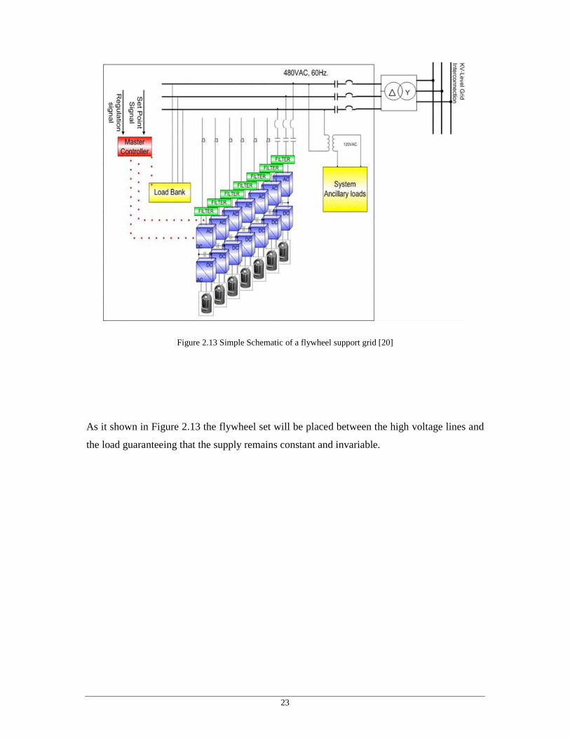
Another project that also has been developed is the “Flywheel – based solutions for grid

Reliability”. This project is based on a “flywheel power plant”, which absorbs the energy

when it is greater than the demand and supplies the power grid when the energy is less than

the demand.

Figure 2.12 Diagram exemplify of the supply and Demand [20]

As it can been seen in the Figure 2.12 the supply must fulfill the demand. When the supply

does not fulfill exactly the demand, it results on a frequency oscillation. The main purpose of

this project is to construct a power plant with a flywheel matrix that stores the energy when

the energy generated is greater than the energy demand. Otherwise, it supplies the system

when the energy generated is not enough to satisfy the demand.

23

Figure 2.13 Simple Schematic of a flywheel support grid [20]

As it shown in Figure 2.13 the flywheel set will be placed between the high voltage lines and

the load guaranteeing that the supply remains constant and invariable.

25

Chapter 3

Flywheel Design Principles 3 Flywheel Design Principles

This chapter provides the design principles of a flywheel’s rotor. A flywheel’s rotor is an

object that rotates at a certain velocity with a certain mass that will store energy by its speed

and mass. The rotor that can be also called the wheel, has been composed, in the past, by iron

and other classical materials but new achievements in engineering with carbon based fibres

will make the wheel less heavy and with the ability to support much higher speeds. This issue

will be further discussed in this chapter, which focuses on the design fundamentals of the

wheel.

26

3.1 General introduction to the magnetic bearing

From the high price of fossil energy in the earliest 21st century, came the conclusion that is

necessary to find another way to power vehicles and other applications. Flywheels may be a

good solution but it’s required a first study of its shape and mass, to have a better view of its

applications. Another important factor is the speed; there must be a balance between speed,

mass and size, which is expressed in order to flywheel’s rotor outer radius.

Another problem in the design of the flywheel is the materials used on the rotating mass. It’s

known that materials like iron and other classic materials don’t have the strength to hold high

rotation speeds. The solution may be the new carbon composite materials due to their higher

resistance to twist forces than the iron and other classic materials.

3.2 Theoretical approach of flywheel’s rotor design

3.2.1 Design fundamental equations

• Fundamental equations

The energy storage in a flywheel system is given by the equation (3.1), where E is the kinetic

energy stored, J is the moment of inertia and w the angular speed of the flywheel.

2

2

1ω⋅⋅= JE (3.1)

27

The moment of inertia is a function of its shape and mass, given by equation (3.2):

2rdmdJ ⋅= (3.2)

For the common solid cylinder, the expression for J it’s given by equation (3.3), where h is

the length of the cylinder, r is the radius and ρ is the density of the cylinder’s material.

ρπ ⋅⋅⋅⋅= hrJ 4

2

1 (3.3)

The other dominating shape is a hollow circular cylinder, approximating a composite or steel

rim attached to a shaft with a web, which results on equation (3.4).

( )44

2

1io rrhJ −⋅⋅⋅⋅= ρπ (3.4)

Where ro is the outer radius and r i is the inner radius.

Then, in equation (3.5), there is the energy (in [MJ]) that can be stored in a flywheel system in

function of its speed and inner and outer radius.

EMJ =14⋅ π ⋅ h ⋅ ρ ⋅ ro

4− ri

4( )⋅ω 2 (3.5)

As a result of equation (3.1), the most efficient way to increase the energy stored in a

flywheel is to speed it up. However, there is a problem with this solution, the materials that

composes the wheel of that rotating system will limit the speed of the flywheel, due to the

28

stress developed, called tensile strength, σ.

• Analysis of stress forces:

The analysis of the stress forces is an important factor in the wheel’s dimensioning. The

tensile strength of a rotation system is composed by two kinds of forces, the radial and the

tangential stresses, respectively σr and σt.

By considering a wheel with uniform thickness and density ρ (figure 3.1), the centrifugal

force acting on an element of the disc can be written as follows [26]:

dFc = dm⋅ r ⋅ω 2= ρ ⋅ h ⋅ r 2

⋅ dϕ ⋅ dr ⋅ω 2 (3.6)

Figure 3.1. Forces and constraints in a wheel with uniform thickness. [26]

By considering the separate element of the disc (figure 3.1.b), the following relation

was obtained [26]:

σ r + dσ r( )⋅ r + dr( )⋅ dϕ −σ r ⋅ r ⋅ dϕ −2⋅σ t ⋅ dr ⋅ sindϕ2

+ ρ ⋅ h ⋅ r 2 ⋅ dϕ ⋅ω 2 = 0 (3.7)

From figure 2.1 and equation (3.7) it was possible to obtain the stresses, for a hollow

29

cylinder with an isotropic material. The radial stress is represented by equation (3.8) and the

tangential stress (also known as hoop stress) is represented by equation (3.9) [5, 32].

( )

−⋅−+⋅⋅⋅+= 2

2

22222

8

3r

r

rrrr

vr io

ior ωρσ (3.8)

( )

⋅+

⋅+−⋅++⋅⋅⋅+= 22

22222

3

31

8

3r

v

v

r

rrrr

vr io

iot ωρσ (3.9)

Where ν is the Poisson ratio, which is a constant of the material of the rotor (this ratio

is described in Annex A).

The next figure shows an example intended to help the understanding of the radial and

tangential stresses.

Figure 3.2. Radial and tangential stress in a short hollow cylinder rotating about its axis with

angular velocity ω. [5]

3.2.2 Inner radius, outer radius and rotation speed relations

In order to dimension the rotor piece, a study of the relation between the outer radius and the

inner radius and the stress forces relationship is required to dimension the wheel.

30

Using equations (3.8) and (3.9), the radial and tangential stress tensions in order to ri

ro

can be

achieved by:

σ r = 3+ v

8⋅ ρ ⋅ω 2 ⋅ ro

2 + ri2 − ro

2 ⋅ ri2

r 2 − r 2

= 3+ v

8⋅ ρ ⋅ω 2 ⋅ ro

2 ⋅ 1+ ri2

ro2 − ri

2

ro2 ⋅ ro

2

r 2 − r 2

ro2

⇔

⇔ σ r

ρ ⋅ω 2 ⋅ ro2 = 3+ v

8⋅ 1+ ri

2

ro2 − ri

2

r 2 − r 2

ro2

(3.10)

σ t = 3+ v

8⋅ ρ ⋅ω 2 ⋅ ro

2 + ri2 + ro

2 ⋅ ri2

r 2 − 1+ 3⋅ v

3+ v⋅ r 2

⇔ 3+ v

8⋅ ρ ⋅ω 2 ⋅ ro

2 ⋅ 1+ ri2

ro2 + ri

2

r 2 − 1+ 3⋅ v

3+ v⋅ r 2

ro2

⇔

⇔ σ t

ρ ⋅ω 2 ⋅ ro2 = 3+ v

8⋅ 1+ ri

2

ro2 + ri

2

r 2 − 1+ 3⋅ v

3+ v⋅ r 2

ro2

(3.11)

Using equations (3.10) and (3.11) and setting 0r

ri with different values, it was made a study

about the values of 22

o

t

r⋅⋅ωρσ

and 22

o

r

r⋅⋅ωρσ

, represented in the next graphic, considering

a=ri

r0

.

31

Figure 3.3. Stress tension variations along the rotor for a=0.2; a=0.5 and a=0.7.

Looking to the variation of ri

ro

, it can be concluded that the tangential stress is always more

important than the radial stress, which makes the tangential stress the most critical one.

As it was shown in figure 2.3, the maximum of the tangential stress is approximately 1, which

yields in equation σ t

ρ ⋅ω 2⋅ ro

2≈1.

For a limited σt, σt =825MPa (which is half of the maximum admitted, for security reasons),

the outer radius and the rotation speed are related and when the outer radius is chosen, the

flywheel speed is limited, as the next graphic expresses.

32

Figure 3.4. Relation between the outer radius and the rotor’s speed, for carbon AS4C.

• Using the achieved tangential stress approximation on the flywheel’s fundamental

equations:

The find of the maximum that maximizes the equations (2.8) and (2.9) is an important factor

for the study of tensile stress.

The maximum of equation (2.8) is on r = ro2⋅ ri

24 and then it can be conclude that

σ r ,max =3+ v

8⋅ ρ ⋅ω 2 ⋅ ro − ri( )2

.

Equation (3.9), gets critical when r=ri,. So, the critical equation is given by (3.12):

⋅

+⋅+−+⋅⋅⋅⋅+=

2

22max 3

3112

8

3

o

iot r

r

v

vr

v ωρσ (3.12)

33

Using the approximation σ t

ρ ⋅ω 2⋅ ro

2≈1, in equation (3.5), the energy limit (in [MJ]) can be

achieved:

Elim = 14

⋅ π ⋅ h ⋅ 1− ri

ro

4

⋅ ro

2 ⋅σ t (3.13)

Taking into account the consideration above, the energy limit per total volume (in [MJ/m3]) is

given by the next equation (with a=ri

ro

):

( ) tvolumeper aE σ⋅−⋅=4

_lim_ 14

1 (3.14)

The energy limit per total volume of rotating mass (in [MJ/m3]) is represented by equation

(3.15):

( ) ( ) ( ) ( ) ttt

massvolumeper aa

aa

a

aE σσ

σ⋅+⋅=⋅

−

+⋅−⋅=

−

⋅−⋅= 2

2

22

2

4

__lim_ 14

1

1

11

4

1

1

1

4

1 (3.15)

Having now these two equations (represented on the next graphic), it is possible to find the

ideal relation between the inner radius and the outer radius, a=ri

ro

.

34

Figure 3.5. Representation of energy limit per total volume, at blue (1+a2) and energy limit

per total volume of rotating mass, at red (1-a4).

It can be seen that the best relation between the inner radius and the outer radius is around

0.7; this value will be confirmed in the next calculations.

• Calculation to find the best relation between the inner radius and the outer radius,

a=ri

ro

:

To find the best relationship between ir and 0r , it’s very important to maximize the

relationship between the wheel volume and its mass.

With α =12

, to obtain the best relation between energy per unit of mass and energy per unit

of volume the equation above results in:

( ) ( )24 112 aaF ++−=

This equation will now be derived in order to obtain the maximum value of a:

( ) ( ) ( )24 111 aaF +⋅−+−⋅= αα

35

2

2

2

1024 23 =⇒=⇒=⋅+⋅−= aaaa

da

dF

It can be concluded that the best relation between the inner radius and the outer radius is 2

2.

3.2.3 Flywheel rotor’s geometry and materials

• Relation between the energy storage capability and the flywheel geometry:

The speed is limited by the stress developed in the wheel, called tensile strength, σ.

A more general expression for the maximum energy density, valid for all flywheel shapes, is

given in equations (3.16) and (3.17), which were obtained from [5].

ev = K ⋅σ (3.16)

em =K ⋅σρ

(3.17)

Where ev is the kinetic energy per unit volume and em per unit mass, K is the shape factor, σ is

the maximum stress in the flywheel and ρ is the mass density. The shape factor K is a constant

that represents the cross section geometries and its value is less than 1, as shown in table 3.1.

The adopted flywheel geometry was a hollow cylinder. This geometry was chosen due to its

simpler manufacture and lower cost, when compared with other geometries.

36

Table 3.1. Shape factor K for different planar stress geometries. [25]

Since the hollow cylinder is not represented in the table, the chosen value for its shape factor

was the same as the thin firm (K=0.5), because it’s the one that has a similar geometry.

• Rotor materials:

The materials that compose the flywheel’s rotor will limit its rotational speed, due to the

tensile strength developed. Lighter materials develop lower inertial loads at a given speed,

therefore composite materials, with low density and high tensile strength, are excellent for

storing kinetic energy.

Table 3.2 shows several materials used on wheels. The analysis of the table confirms that the

carbon composite materials are the ones that maximize the energy density.

Composite materials are a new generation of materials that are lighter and stronger than the

conventional ones, like steel.

For the simulations it was chosen carbon AS4C because it is the second best on tensile

37

strength and on energy density and less than a half of the price of the first one.

Table 3.2. Characteristics for common rotor materials. [27]

3.3 Flywheel rotor’s dimensions, weight and material’s cost

The relation that maximises energy with less material and speed will be now applied to design

a wheel that can be used in a flywheel system application.

To the design of a flywheel rotor’s dimensions, weight and material’s cost, some calculations

were made and are represented in Annex 2, starting with the 1st series of calculations (which

was the most successful one) until the 4th series of calculations.

To calculate the rotor’s weight, the density of ρ=1510Kg/m3 was used, and to calculate the

material’s cost, the carbon price of 31,3 $ /Kg was used (values taken from table 3.2).

The series of results achieved in Annex B were compared with the weight and volume of each

wheel, as table 3.3 shows.

38

Table 3.3. Rotor’s dimensions, weight and material’s price for different energy capacities.

Elim N

(rpm) ro (m) ri (m) h (m)

Occupied

volume

(m3)

Material’s

volume

(m3)

Weight

(Kg)

Material’s

cost ($)

2.5 kWh; 9MJ 33613 0.21 0.148 0.42 0.06 0.03 44 1385

2.5 kWh; 9MJ 42350 0.167 0.118 0.667 0.06 0.03 44 1385

1kWh; 3.6MJ 45620 0.155 0.109 0.31 0.02 0.01 18 558

25 kWh; 90MJ 15602 0.452 0.32 0.905 0.6 0.3 438 13706

0.44kWh; 1.58MJ 60000 0.118 0.083 0.235 0.01 0.005 8 245

By the analysis of table 3.3, the most interesting results are the 1st and 4th series of

calculations (lines 1 and 2 of the table). It can be concluded that the energy depends on the

gyrating volume and not directly on the rotor’s radius and height. As it can be seen, both 1st

series and 4th series have a wheel with the same energy capability storage, the same mass and

the same price. It is also shown that in the 4th series it occupies more space and still needs to

spin faster than in the 1st series.

Based on the results shown in table 3.3, a flywheel energy-storage system with 5 kWh

capacity could be designed for the application on an electric vehicle, having two robust rotors

of 2,5 kWh, each one, and the transformation between rotational kinetic energy and electrical

energy would be performed with two permanent magnet motor/generator of 30 kW (40.23 hp)

each.

It was chosen to use two rotors of 2,5 kWh instead of one rotor of 5 kWh, in order to fit the

free area inside an automobile.

Using the 1st series of calculations, each rotor has a mass of 44 kg and uses a carbon-fibre

composite rim (for the two rotors, the material’s cost is around $3000), combined with a solid

39

metallic hub, to create a rotor without critical resonances within the normal operating range.

3.4 An example for the use of the wheel

Based on the section 3.3 results, according to the wheel design and its energy capability, a

wide range of applications for the wheel can be defined and imagined, one of them could be

an electrical system that needs great power capability, as for instance, a flywheel energy

system bus.

For this system, electrically, the motor/generator of each flywheel could be connected to the

same dc bus through its own inverter and filter, as shown in figure 3.6.

Figure 3.6. Electrical schematic of the two flywheels connection. [2]

In charge mode, the dc current Iflywheel is positive and the speed of the flywheels is increasing.

In discharge mode, the flywheels are decreasing in speed and providing power to the dc bus.

From figure 3.6 it can be concluded that this implementation maintains both flywheels with

the same amount of energy.

40

An example of one of the flywheels used on the system above is shown in figure 3.7.

30 kW Motor / Generator

Composite Rotor / Metallic Hub

Bearing Suspension

Figure 3.7. Cutaway view of a flywheel energy-storage system. [3]

The flywheel energy-storage system represented in figure 3.7 will have rotor of 2,5 kWh and

a permanent magnet motor/generator of 30 kW (40.23 hp). The rotor will have a mass of 44

kg and the material’s cost will be around $1400.

41

Chapter 4

Design of a magnetic bearing:

general approach 4 Design of a magnetic bearing: general approach

This chapter describes the process used to design a magnetic bearing. In this chapter, the

structure and constitution of an electromagnetic bearing is studied taking into account the

results obtained in chapter 3. The proposed solution has a vertical structure joining together

two types of magnetic circuits: a passive circuit and an active circuit. The characteristics of

these circuits will be analysed and discussed, mainly the constitutive aspects that unbalance

the system.

42

4.1 General introduction to the magnetic bearing

In the constitution of a magnetic bearing it is possible to identify two types of circuits, as it is

described in chapter 2: an active circuit or/and a passive circuit.

As it was referred in chapter 2, it is possible to identify several solutions for magnetic

bearings depending on the power, speed, application and performance. In this work the

flywheel is designed either for an industrial application or domestic power application.

Furthermore the aspects above, the magnetic bearing can be designed having a vertical

structure or/and with a radial structure. In this work a magnetic bearing with a vertical

structure is studied, in agreement with the results of chapter 3. According to the results

described in the previous chapter, the design of the magnetic bearing should fulfil the

following requirements:

• Energy: 9 MJ

• Radius of 0.148 m

• Support weight of 45 kg + 30 % (motor and magnetic circuit in the wheel)

Taking into consideration all these aspects and parameters, this chapter describes the process

used to design a magnetic bearing. In the proposed solution, the energy losses, bearing cost

and planning aspects are also analysed.

4.2 Generic structure of the magnetic bearing

A magnetic bearing sustains loads using the magnetic levitation principle. It is an object that

creates a magnetic field that levitates, for example, rotating shafts. The magnetic bearing, that

43

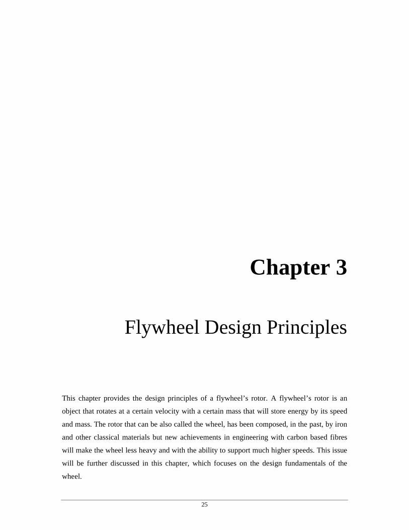
will be implemented, has two magnetic circuits, the active and the passive one. They have two

different functions. The main function of the passive magnetic circuit is to compensate the

weight of the wheel. The active circuit (with or without a position sensor) has the function of

compensating the instability in the system, without the active bearing the system can be

unstable. In order to exemplify the constitution of a bearing, the basic structure of a flywheel

with a magnetic bearing is shown in Figure 4.1.

Figure 4.1 Flywheel with a magnet bearing [7]

Figure 4.1 illustrates a bearing with a vertical axis, as it will be designed in this work. This

magnetic bearing will support the wheel, which includes a synchronous machine that has been

studied in this work [28].

This basic system represented in Figure 4.1 corresponds to a flywheel with a vertical structure

(same structure of the proposed solution with this work). In addition to the elements referred,

Figure 4.1 also shows the rotor/generator element, which is a synchronous machine according

[28]. When designing the magnetic bearing the weight of the electric machine is an important

factor (20 % of the total weight).

44

4.2.1 The permanent magnet

The passive bearings have at least one permanent magnet. As it was shown in chapter 2, there

are several types of magnets that can be used. Anyway, the neodymium iron boron magnet is

the best solution for the current application. A permanent neodymium iron boron magnet

gives the magnetic flux necessary to sustain the system and to centre the moving pieces. It is a

good solution because there are no energy losses, but there is no dynamic control of the flux

density. So, it is not possible to control the position of the rotating mass. Despite this factor,

the permanent magnet is the ideal solution for sustaining the rotor in the ideal conditions,

there is, without any disturbance in the wheel.

4.2.2 General Description of the active bearing

For a flywheel with an active bearing, it is possible to design and adapt their functionalities

according to different point of views, being the most important the following one:

• The position of the active circuit: the placement of the active circuit can be done

keeping in mind that the main functions of the AMB are to levitate, align and sustain

the rotating mass of the flywheel.

A coil placed inside the active bearing structure constitutes the active circuit of the AMB.

This coil is supplied by a controlled current source. The section available to place the coil

depends on the global characteristics of the bearing (referred in point 4.1). This section is a

restriction when designing the AMB (it is physically limited). In addition, being the coils

encapsulated, heat dissipation problems can occur. So, the number of coil turns and the wire

section should be dimensioned taking into account these restrictions and fulfilling the

functionalities of the AMB.

Having a magnetic bearing with an active circuit, it is possible to control the position of the

rotating mass. The control of the position is typically based on a position sensor, which has an

important role in this type of system. It is important to point out that a flywheel requires an

adequate control system controlling not only the AMB circuits but also the electrical machine

of the flywheel (the aspects of the control system are not studied in this work).

45

4.3 Adopted Solution

Taking into account the restrictions, the requirements and the tools available to design and to

implement a magnetic bearing a solution with the following basic structure was chosen and

studied.

Figure 4.2 Shape of the basic structure of the magnetic bearing [7].

The model shown in Figure 4.2 is similar to the solution presented in reference [7]. This

solution, when compared to others [8, 11, 19 and 27] seems simpler. Anyway, it fulfils the

requirements of a magnetic bearing framed by the parameters referred in point 4.1. In

addition, the proposed solution is less expensive when compared to similar solutions.

To describe the proposed solution, four main elements should be analysed and studied: the

teeth, the magnet, the rotor and the coil.

• Teeth: Slots have been used in magnetic circuits with the purpose of influencing the

flux density distribution. The flux lines distribution depends on the placement of the

moving pieces in the electromagnetic system (similar situations are verified in

flywheels). In this work slots will be named teeth as in [7].

• Magnet: It should have an appropriate design in order to guarantee contact free

between the rotor and the bearing and to better balance the wheel (rotor). The magnet

is the main part of the PMB. It will be positioned between the coil and the slots

(teeth) in order to achieve the best force distribution.

• Rotor: Attached to the carbon-fibre wheel (discussed in chapter) 3 there will be a

46

magnetic material, with the purpose of closing the magnetic circuit.

• Coil: This element belongs to the AMB having a cylindrical shape. It is closer to the

outer radius in order to maximize the area where the copper wire can be placed. It is

constituted by a copper wire that creates a flux density supporting the passive bearing.

The coil is supplied by a controlled current source.

The solution described above is a part of the system shown in Figure 4.3. The system has two

magnet bearings: an upper bearing and a downward bearing.

-

Figure 4.3 Schematic chosen for the design of the magnetic bearing [7].

From Figure 4.3 it is possible to identify the three main components of the system under

study: upper bearing, downward bearing and rotor (white). The purpose of this chapter is to

design the upper bearing and the downward bearing.

It is important to refer that the magnet of the downward bearing is only for centring purpose.

So, the magnet of the upper bearing will have to sustain the wheel and compensate the force

that the downward magnet exercises on the wheel.

47

4.3.1 Generic aspects of the standard bearing

In order to design a magnetic bearing, a model equivalent to the system shown previously

(Figure 4.2) was built using the software Fem 4.0™. The first model implemented using the

FEMM 4.0TM, was called standard bearing, having a radius of 14.8 cm, which is the wheel

inner radius obtained in chapter 3. The model simulated is built of iron with a permanent

magnet of neodymium iron boron and a coil with copper wire with 1mm of diameter, as

indicated in the figure.

Figure 4.4 Schematic of the magnetic bearing using FEMM.

4.3.2 Standard bearing dimensions

According to the point 4.1 descriptions, it is known that the radius of the bearing is 0.148 m.

So, using their parameters as reference, the other dimensions of the bearing were obtained re-

scaling the information available in article [7]. Figure 4.5 shows the dimensions that were

used on the simulations of the standard bearing.

48

Figure 4.5 Dimension of the bearing (L1=4 cm; L2=2.3cm; L3=1.8 cm; L4=4.9 cm; L5=2.7 cm; L6=9.9 cm;

L7=2mm; L8=0.9 cm; L9=0.9 cm; L10= 5.8 cm; L11= 4.1 cm; L12=2.7 cm; L13=2.7 cm; L14=3.1 cm; L15=3.6

cm ;L16=5.3 cm; L17=1.3 cm; L18=2.7cm; L19=0.9 cm; L20=9 cm).

4.3.3 Flux density distribution for the standard bearing

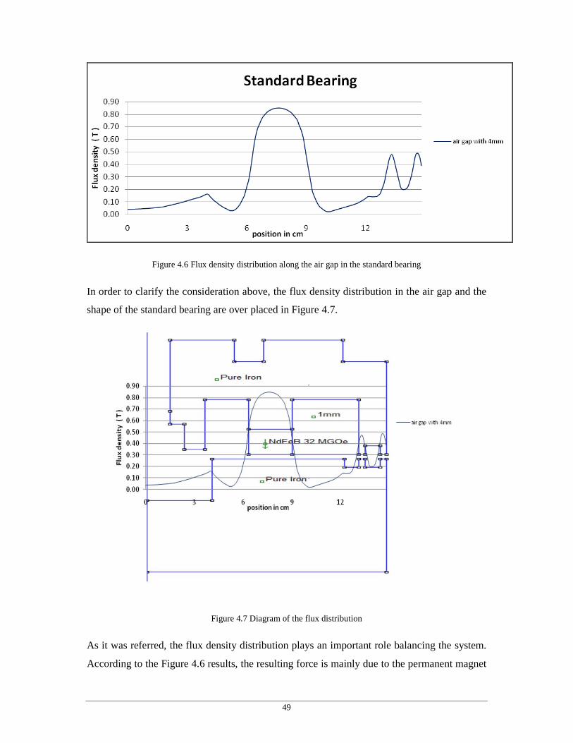
From the standard magnetic bearing simulated using FEMM, the flux density distribution, in

the air gap was obtained (Figure 4.6). As it can be seen, the flux density reaches significant

values in the air gap near the magnet and on the teeth air gap. As it was expected, the size of

the air gap, the magnet dimensions and the teeth influence the flux density amplitude and

distribution. Furthermore, the placement of the permanent magnet and the teeth also influence

the flux density distribution along the air gap.

49

Figure 4.6 Flux density distribution along the air gap in the standard bearing

In order to clarify the consideration above, the flux density distribution in the air gap and the

shape of the standard bearing are over placed in Figure 4.7.

Figure 4.7 Diagram of the flux distribution

As it was referred, the flux density distribution plays an important role balancing the system.

According to the Figure 4.6 results, the resulting force is mainly due to the permanent magnet

50

and the teeth. Before the study of the influence of the air gap flux density it is important to

know the forces that interact in this system.

As it was referred before, the resulting vertical force in this system must be zero, in order to

guarantee the levitation of the wheel and the horizontal force is responsible for the wheel

centring. Furthermore, the flux density distribution is an important factor in order to balance

the forces applied to the system. So, to put the pieces in balance without contact and centred,

the analysis of the flux density distribution is mandatory.

4.3.4 System under study

The resulting force in this system depends on the flux density distribution in the bearing air

gap. Before studying the flux density distribution, it is important to describe the forces present

in this system. The resulting force can be decomposed in two components: the vertical and the

horizontal force. Also the function of each component can be identified.

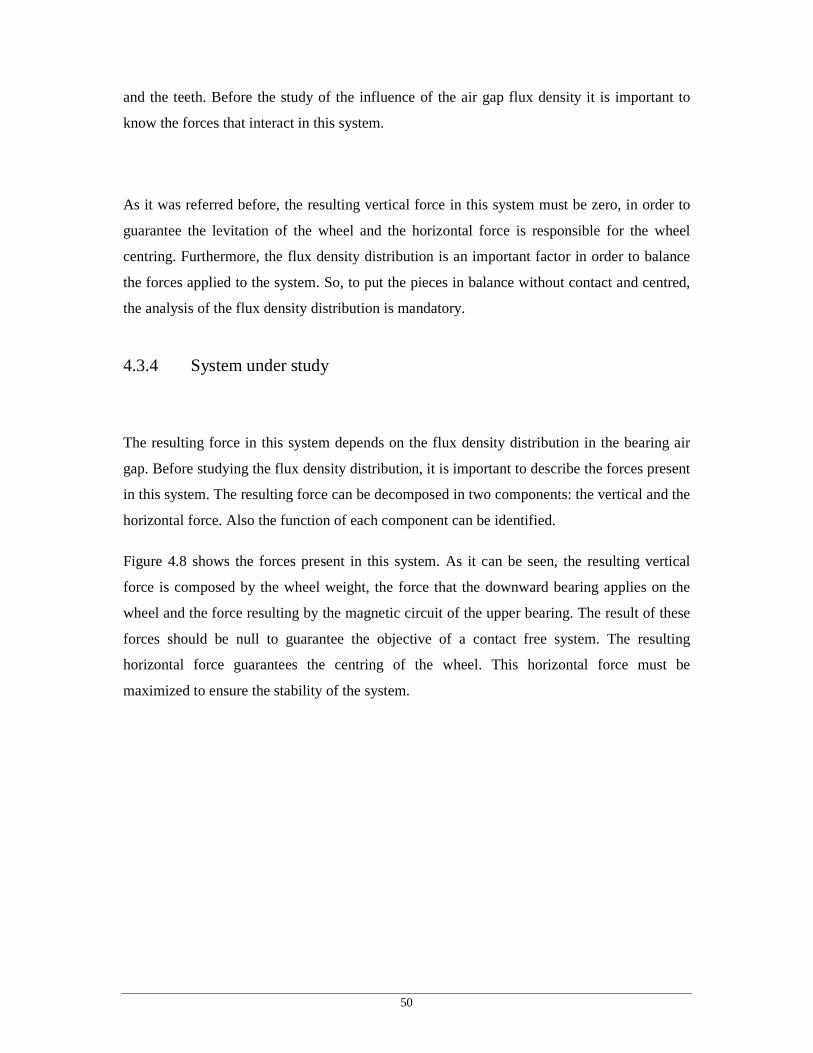
Figure 4.8 shows the forces present in this system. As it can be seen, the resulting vertical

force is composed by the wheel weight, the force that the downward bearing applies on the

wheel and the force resulting by the magnetic circuit of the upper bearing. The result of these

forces should be null to guarantee the objective of a contact free system. The resulting

horizontal force guarantees the centring of the wheel. This horizontal force must be

maximized to ensure the stability of the system.

51

Figure 4.8 Forces applied to the system

The horizontal force should ensure that the instabilities do not change the position of the

wheel. Instabilities can occur due the fringing effect and by the charge or discharge of the

flywheel (speed up/slowing down). Equation 4.1 and 4.2 represent the influence of the force

(vertical effect) and pressure (horizontal effect) of the flux density of the air gap in the

rotating mass.

0

2

µSB

F = (4.1)

0

2

µB

P = (4.2)

As it is known, the flux is related with the flux density and the section, as shown in equation

(4.3):

SB ⋅=φ (4.3)

From equations (4.1) and (4.3) it is possible to verify that the magnetic force in the air gap

depends on the flux and on the section (S) that is perpendicular to the flux density as shown

by equation (4.4):

52

0

2

µφS

F = (4.4)

So, from the equations above it is imperative the study of the flux density in the bearing air

gap, which will be realized further on in this work.

4.4 Teeth and Permanent Magnet

From the previous points, it was verified that the magnetic bearing has two sections (teeth and

permanent magnet) where the flux density has a significant value. With the purpose of better

understanding the influence of the teeth and magnet in the system behaviour, a detailed study

using the equivalent magnetic circuit of this system will be done.

Figure 4.9 shows the magnetic bearing in study. It is important to notice that the bearing has a

cylindrical shape. In order to obtain the magnetic model, several radius in key points of the

bearing were defined.

Figure 4.9 Cross section of the magnetic bearing

From the radius defined above, it becomes possible to obtain the magnetic equivalent circuit

equations. In this way, it is possible to obtain the equations as function of the dimensions.

53

4.4.1 Equivalent magnetic circuit

To study the behaviour of an electromagnetic device, magnetic field paths should be defined,

such as in some confined space, being modelled by a magnetic circuit. When dealing with

machines of not medium size and very high operating frequencies, the displacement current

term is negligible in the integral form of Ampere’s circuit law. For the study of the magnetic

bearing there was a need to create an equivalent circuit including the magnetic reluctances, as

shown in Figure 4.10.

ℑm

ℜmagnet

ℜg1 ℜg22ℜg21

Figure 4.10 Magnetic bearing and its equivalent magnetic circuit

From Ampere’s circuit law equation 4.5 where C is a closed contour and S is any surface

whose edge is defined by C.

∫ ∫ →→→→

⋅=⋅c s

daJdlH (4.5)

In these kinds of applications, the above line integral could be approximated by the following

54

summation:

∑=

=

m

ili IlH

1 (4.6)

Where il is the length of the thi section and I is the net current linked to the flux path.

Similarly, the integral form of the divergence theorem may be expressed as:

0=⋅∫ →→

sdaB (4.7)

The reluctances of the various sections can be determined according to the core dimensions of

the sections. As an example, the air gap reluctance between the magnet and the down piece it

is given by equation (4.8).

( )21

22

1rr

g

og −⋅=ℜ

πµ (4.8)

Where g is size of the air gap between the two pieces, 0µ the permeability of the air and the

expression ( )21

22 rr −π is the section that is orthogonal to the flux density. From equation

(4.8) and using the same method it is easy to get the expressions for the magnetic reluctances

in the teeth air gaps, which are expressed by equations (4.9) and (4.10).

( )23

240

21rr

gg −⋅

=ℜπµ

(4.9)

( )25

26

22rr

g

og −⋅

=ℜπµ

(4.10)

To find the expression of the reluctance in the permanent magnet (equation (4.11)) a similar

method is used;

55

( )21

22 rr

l

A

l

or

m

magnetor

mmagnet −⋅⋅

=⋅⋅

=ℜπµµµµ

(4.11)

In this case ml is the length of the magnet and rµ is the relative permeability of the magnet,

which is for instance 05.1=rµ (permeability similar to the air for the neodymium iron boron

magnet.

The voltage source that represents the magnetomotive force source is represented by equation:

cmm Hl ⋅=ℑ (4.12)

The magnetomotive force ℑm depends of the length of the magnet and of the coercivity field

of the magnet.

The equivalent reluctance of the magnetic circuit is an important factor to better understand

the magnetic behaviour of the system and to better design its components.

From equation (4.10) and (4.11) it can be seen the equivalent reluctance of the teeth magnetic

reluctance in the air gap.

ℜ+ℜ=ℜ− 22212

111

ggequig

(4.13)

( ) ( )( )25

26

23

240

2 −+−⋅=ℜ

−

rrr

gequig πµ

(4.14)

The total equivalent reluctance of the entire magnetic circuit is the sum of its magnetic

reluctances as it is shown in equations (4.15), (4.16) and (4.17).

56

12 gmagnetequigequig ℜ+ℜ+ℜ=ℜ−−

(4.15)

( ) ( )( ) ( ) ( )21

220

21

220

25

26

23

240 rr

g

rr

l

rrrr

g

r

mequig −⋅

+−⋅⋅

+−+−⋅

=ℜ− πµπµµπµ

(4.16)

( ) ( )( ) ( ) ( )( ) ( )( ) ( ) ( )( ) ro

rrmrequig

rrrrrr

rrgrrrrlrrrrg

µπµµµµ

25

26

23

24

21

22

21

22

25

26

23

24

25

26

23

24

−+−⋅−⋅−⋅+−+−⋅+−+−=ℜ

− (4.17)

4.5 Sensibility analysis

With the objective of knowing the influence of teeth size and magnet size on the flux density

distribution of the bearing air gap, a sensibility analysis was made focusing on the teeth size,

magnet size and air gap distance. On these tests the bearing from Figure 4.5, the standard

bearing, will suffer some modifications on its dimensions and then the flux density

distribution on the air gap will be compared with the standard bearing results. Interesting

results were obtained with this analysis, which will be presented in the coming points.

4.5.1 Analysis of the relative position of the pieces

First of all it is important to make the following remark: to analyse the behaviour of the

system, the air gap (“in grey in Figure 4.11) that was taken into consideration in the

simulations is not only the length that separates the two pieces, but also includes the

permanent magnets and the copper coil sections. The relative magnetic permeabilities of the

permanent magnet volume and of the copper volume were considered the same of the air. To

understand the influence of the air gap size in the flux density, different values to the distance

between the two pieces were tested.

57

Figure 4.11 Air gap distance, which was tested for different values

In the Figure 4.12, it is shown the variation of the magnetic field, of the standard bearing, for

different air gap dimensions.

Figure 4.12 Flux density value in the standard bearing

As it can be seen in the figure above, the relative position of the bearing air gap influences the

flux density amplitude in the proximity of the teeth and on the permanent magnet region. The

magnetic field falls to half of its value from an air gap with a 2 mm to an air gap with 7 mm

near the teeth. It can be also seen that the flux density along the rest of the air gap does not

suffer any significant fluctuation with the variation of the air gap width.

Air Gap Variation

58

4.5.2 Analysis of the teeth thickness

The next analysis characterizes the influence of teeth thickness on the air gap flux density. It

is important to understand the influences of the teeth on the flux linkage and, by consequence,

on the magnetic force, because the teeth thickness influences directly its magnetic reluctance.

Figure 4.13 Variation on teeth thickness: a) teeth from standard bearing b) teeth with more 2mm c) teeth with

less 2 mm

In Figure 4.14 the teeth thickness is increased 2 mm as it shown in Figure 4.13 b).

Figure 4.14 Flux density value on 2mm increased teeth

59

The next figure illustrates the result of a 2 mm decrease in teeth thickness (Figure 4.13 c)).

Figure 4.15 Flux density value on 2mm decreased teeth

It can be verified from the analysis above that the teeth thickness variation only influences the

flux density in the small air gap near the teeth. This is an important factor knowing that the

teeth are located near the edge and from equation (4.2), the teeth thickness influences the

force for centring purpose.

4.5.3 Analysis of the influence of the size of the magnet

With the purpose of knowing the influence of the magnet size, simulations changing the

permanent magnet size were performed. The next two figures show the variations of the

magnetic field on different situations: in the first case, the magnet is thicker than the standard

version; in the second case, it is less thick than the standard version; and in the third case, the

magnet has a smaller length than the standard version.

60

Figure 4.16 Different magnets used in the simulations

In the next figure the results of the simulation using the magnet on Figure 4.16 b) are shown.

Figure 4.17 Flux density value on a 7mm magnet bearing

Using the magnet on Figure 4.16 c), the results are:

yr

y3

x3

x2

y2 y1

x1 xr

a)Standard magnet c) Magnet with xr<x2 b) Magnet with xr>x1

d) Magnet with yr>y3

61

Figure 4.18 Flux density on a 4.5 cm thickness bearing

In Figure 4.19 the magnet from Figure 4.16 d) was used.

Figure 4.19 Flux density on a 7mm Lm bearing

With these three simulations it can be pointed out that the magnet size influences strongly the

flux density in the teeth air gap. It is important to realize that changes of the teeth thickness

are very important because they influence significantly the magnet reluctance.

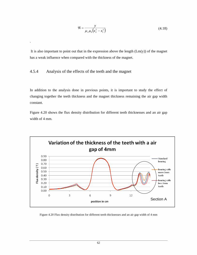
62

( )21

220 xx

y

r −=ℜµµ

(4.18)

.

It is also important to point out that in the expression above the length (Lm(y)) of the magnet

has a weak influence when compared with the thickness of the magnet.

4.5.4 Analysis of the effects of the teeth and the magnet

In addition to the analysis done in previous points, it is important to study the effect of

changing together the teeth thickness and the magnet thickness remaining the air gap width

constant.

Figure 4.20 shows the flux density distribution for different teeth thicknesses and an air gap

width of 4 mm.

Figure 4.20 Flux density distribution for different teeth thicknesses and an air gap width of 4 mm

Section A

63

From the analysis of the Figure 4.20 it is possible to conclude that, as it was expected, the

variation in the teeth thickness if not very significant. Anyway, the teeth thickness influences

the flux density in the air section where the teeth are placed (section A of Figure 4.20).

Furthermore, the most important remark is that the thickness of the teeth is important to align

the rotor (wheel) but that issue will be further discussed in detail.

Figure 4.21 Flux density distribution for different magnet thicknesses and an air gap width of 4 mm

In order to study the influence of the magnet size in the air gap flux density distribution,

Figure 4.21 shows the effect of changing the permanent magnet thickness, for a constant air

gap. These variations influence the flux density distribution in the air gap and, for that reason,

the vertical force. So, it is an important factor in the levitation of the wheel. It is important to

point out that the magnet thickness influences clearly the flux density amplitude in the teeth

air gap section.

The next figure shows the variation of the magnet length. As it can be observed that the

effects are not so significant as in the previous case because this variation has not a significant

effect in the magnetic reluctance related with the permanent magnet.

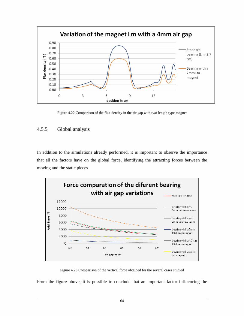
64

Figure 4.22 Comparison of the flux density in the air gap with two length type magnet

4.5.5 Global analysis

In addition to the simulations already performed, it is important to observe the importance

that all the factors have on the global force, identifying the attracting forces between the

moving and the static pieces.

Figure 4.23 Comparison of the vertical force obtained for the several cases studied

From the figure above, it is possible to conclude that an important factor influencing the

65

system behaviour is the thickness of the magnet. Small adjustments can be done to reach the

specifications defined in chapter 3 by changing the teeth thickness and the air gap size.

4.5.6 Analysis with planar geometry

The analysis done before does not give any information if a small shift occurs in the wheel

position and therefore, the effect on the air gap flux density distribution. As it was referred

before, the teeth have an important function in maintaining the wheel centred. For that

purpose another analysis is required in order to better design the bearing teeth. The next

simulations focus on the hypotheses that a small shift occurs in the wheel.

Being the model implemented in a 2 D, in the coming simulations, a change in geometry was

made because of the FEMM 4.0TM axisymetrical limitations. It was used a planar geometry,

meaning that peace is no longer cylindrical but has a cubic form.

In this case, the geometry is planar and the absolute force values may not be accurate but the

relations between forces and bearing shape are valid.

In Figure 4.24, increments of 2 mm in the teeth thickness (growing in the radial outer

direction) were tested and the effects in the axial force were estimated.

-16

-14

-12

-10

-8

-6

-4

-2

0

0 0.2 0.4 0.6 0.8

x axia

l force

(N)

air gap in cm

Wheel with a 2mm diversion from the center

teeth with 4mm thickness



Figure 4.24 Comparison of the horizontal force values for different teeth thickness

66

As it can be observed in Figure 4.24 for air gap distances less than 4 mm, due to the

dispersion caused by the distance between the two pieces of the bearing, the force distribution

is different from teeth thickness to teeth thickness. For air gaps over 4 mm, it can be observed

a little difference between the several situations simulated.

The resulting force in the wheel can be represented by a second order polynomial approach.

The expressions obtained for each teeth dimension are the following:

• 4mm teeth

414.30427.9844.81)( 2 −+⋅−= xxxy (4.19)

• 6mm teeth

982.19017.62182.50)( 2 −+⋅−= xxxy (4.20)

• 2mm teeth

284.18871.56447.45)( 2 −⋅+⋅−= xxxy (4.21)

In the equations above, the axial force (y) is represented as function of the air gap width )(x .

So, we can assume that the axial force can be represented in a general form by:

32

22

1)( kxkxkxy +⋅+⋅−= (4.22)

The coefficients 1k , 2k and 3k depend on the general dimensions of the magnetic bearing.

In addition, it is also important to study the flux density distribution in the air gap, when shifts

in the wheel position occur. The next simulations show the flux density in the air gap with

67

several wheel diversions.

0.00

0.10

0.20

0.30

0.40

0.50

0.60

0.70

0.80

0.90

0 3 6 9 12 15 18 21 24 27 30

Flux d

ensit

y (T)

position in cm

Bearing with teeth of 4mm 0mm diversion 1mm diversion 2mm diversion 3mm diversion 4mm diversion 5mm diversion

Figure 4.25 Flux density value with several shifts with 4mm teeth

It can be seen in Figure 4.25, the flux density in the air gap under the teeth is not constant due

to the changes of the wheel position. Anyway, but for the other zones of the bearing air gap,

the magnetic field remains constant. So it can be concluded that the wheel position affects

mainly the air gap in the teeth section.

0.000.100.200.300.400.500.600.700.800.90

0 3 6 9 12 15 18 21 24 27 30

Flux d

ensit

y (T)

position in cm

Bearing with teeth of 2mm0mm diversion 1mm diversion 2mm diversion 3mm diversion 4mm diversion 5mm diversion

Figure 4.26 Flux density value with several shifts with 2 mm teeth

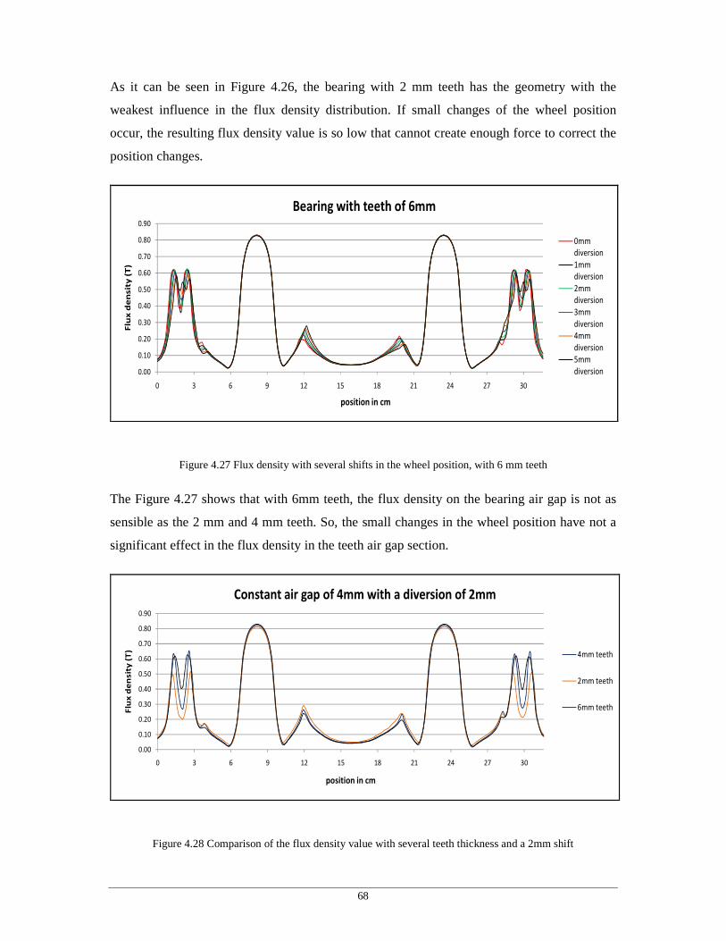
68

As it can be seen in Figure 4.26, the bearing with 2 mm teeth has the geometry with the

weakest influence in the flux density distribution. If small changes of the wheel position

occur, the resulting flux density value is so low that cannot create enough force to correct the

position changes.

0.00

0.10

0.20

0.30

0.40

0.50

0.60

0.70

0.80

0.90

0 3 6 9 12 15 18 21 24 27 30

Flux d

ensit

y (T)

position in cm

Bearing with teeth of 6mm0mm diversion 1mm diversion 2mm diversion 3mm diversion 4mm diversion 5mm diversion

Figure 4.27 Flux density with several shifts in the wheel position, with 6 mm teeth

The Figure 4.27 shows that with 6mm teeth, the flux density on the bearing air gap is not as

sensible as the 2 mm and 4 mm teeth. So, the small changes in the wheel position have not a

significant effect in the flux density in the teeth air gap section.

0.00

0.10

0.20

0.30

0.40

0.50

0.60

0.70

0.80

0.90

0 3 6 9 12 15 18 21 24 27 30

Flux d

ensit

y (T)

position in cm

Constant air gap of 4mm with a diversion of 2mm

4mm teeth

2mm teeth

6mm teeth

Figure 4.28 Comparison of the flux density value with several teeth thickness and a 2mm shift

69

The analysis above shows a small change in the wheel position (2 mm) and the flux density

value in the bearing air gap. It also shows that the peak value is greater with 4 mm teeth than

with 6 mm teeth.

0.00

0.10

0.20

0.30

0.40

0.50

0.60

0.70

0.80

0.90

0 3 6 9 12 15 18 21 24 27 30

Flux d

ensit

y (T)

position in cm


4mm teeth

2mm teeth

6mm teeth


In this situation it can be seen that the peak of the flux density value is more or less the same

for a 4 mm teeth or a 6 mm teeth.

0.00

0.10

0.20

0.30

0.40

0.50

0.60

0.70

0.80

0.90

0 3 6 9 12 15 18 21 24 27 30

Flux d

ensit

y

position in cm


4mm teeth

2mm teeth

6mm teeth


In Figure 4.30, a significant change in the wheel position is illustrated (4 mm). The amplitude

of the flux density value for 6 mm teeth is greater than with 4 mm teeth. As it was expected,

70

bigger teeth are more sensible to strong changes in the wheel position.

4.5.7 Global analysis of the teeth influence

To summarize the influence of the teeth thickness on the wheel stability, the Figure 4.31

shows the comparison between the several teeth thickness and with several shifts from the

centre.

-6

-5

-4

-3

-2

-1

00 0.05 0.1 0.15 0.2 0.25 0.3 0.35 0.4 0.45 0.5

xx's

Fo

rce

(N

)

diversion in cm

Resulting Force of the diversion of the wheel 4mm teeth

2mm teeth

6mm teeth

Figure 4.31 Comparison of the horizontal force with several teeth thickness

The 2 mm teeth are more sensible to smaller changes due to the bigger magnetic reluctance

but according to Figure 4.25, Figure 4.26 and Figure 4.27 the magnetic field is very small. So

it cannot produce enough horizontal force to move the wheel to its original position.

With 6 mm teeth, it can be only observed a significant horizontal force when significant

wheel position changes occur. Anyway, for significant position changes the bearing suffers

also the influences of the active circuit.

So it can be concluded that for small position changes, symmetrical teeth is the best solution,

because the active part of the bearing will correct the instabilities or decentring effects. For

smaller adjustments of the wheel, the 4 mm teeth are the best solution.

71

4.6 Global approach

Analysing the results presented in previous points it can be clearly verified the importance of

the permanent magnet and the teeth in this system. Furthermore, the previous equivalent

magnetic circuit was obtained joining the contributions of all the magnetic sections belonging

to the magnetic bearing.

Taking into account the goals of this work, the previous results lead to the simplification of

the equivalent magnetic circuit.

The simplified equivalent magnetic circuit is composed by four magnetic reluctances and a

magnetomotive force as shown in Figure 4.32.

Figure 4.32- Equivalent magnetic circuit

With this equivalent magnetic circuit it is possible to calculate the flux density in the air gaps

using the magnetic reluctance expressions obtained before, which are the same.

The flux density depends of the flux (Φ) and the section of the air gap (A) (Equation 4.23).

The flux can be represented by Equation (4.24), as function of the magnetomotive force and

the equivalent magnetic reluctance ( equig−ℜ defined in equation 4.17).

72

(4.23)

(4.24)

With equations (4.23) and (4.24) it is possible to represent the flux density as function of the

dimension of the bearing, the magnet reluctances and from the mmf. Equations (4.25)

represents the flux density in the air gap surface under the permanent magnet; Equation

(4.26) the flux density in the air gap surface between the inner teeth and Equation (4.27) the

flux density in the air gap surface between the outer teeth.

(4.25)

(4.26)

(4.27)

Using the equations above and for several air gap widths simulated with FEMM the results of

the flux density in the air gap, comparison were made using the different results.

The next figures show the comparison of the flux density in the magnet air gap using FEMM

and MATLAB.

73

Figure 4.33 Flux density near the permanent magnet using the two methods

Figure 4.33 shows that there is no significant difence between the results from FEMM and

from MATLAB. This represents that the model of the equivalent magnetic circuit near the

magnet air gap is a good representation of the system itself.

The following figure (Figure 4.34) shows the several results using of the flux density in the

inner teeth air gap.

Figure 4.34 Values of the flux density using FEMM and MATLAB between the inner teeth

74

Figure 4.34 shows a significant diference between the two methods. The results from

MATLAB are the double of the values obtain with FEMM. This an important result that will

be taken into account when dimensioning the system further on in this work.

Figure 4.35 Values of the flux density using FEMM and MATLAB between the inner teeth

Figure 4.35 shows the same anomaly as the flux density in the inner teeth. This represents that

the flux in the equivalent system is the double of its true value.

From the results above, it can be concluded that equivalent magnetic circuit near the magnet

represents the system well, the same does not work in the air gap near the teeth, and the flux

density it is half of the value obtained using the equivalent circuit. So, it is important to take

into account this factor and to compare the final dimensions with FEMM. This approximation

can be considered a good result for a preliminary approach.

It is also important for quantifying purpose to known the relative difference of two methods

used in this work. The following figures show the error between the two methods used in this

work.

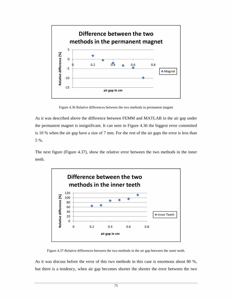
75

-15

-10

-5

0

5

0 0.2 0.4 0.6 0.8Re

lative

diffe

rence

[%]

air gap in cm

Difference between the two methods in the permanent magnet

Magnet

Figure 4.36 Relative differences between the two methods in permanent magnet

As it was described above the difference between FEMM and MATLAB in the air gap under

the permanent magnet is insignificant. It can seen in Figure 4.36 the biggest error committed

is 10 % when the air gap have a size of 7 mm. For the rest of the air gaps the error is less than

5 %.

The next figure (Figure 4.37), show the relative error between the two methods in the inner

teeth.

020406080

100120

0 0.2 0.4 0.6 0.8Relat

ive di

fferen

ce [%

]

air gap in cm

Difference between the two methods in the inner teeth

Inner Teeth

Figure 4.37-Relative differences between the two methods in the air gap between the outer teeth.

As it was discuss before the error of this two methods in this case is enormous about 80 %,

but there is a tendency, when air gap becomes shorter the shorter the error between the two

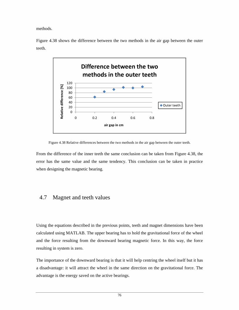
76

methods.

Figure 4.38 shows the difference between the two methods in the air gap between the outer

teeth.

020406080

100120

0 0.2 0.4 0.6 0.8Relat

ive di

fferen

ce [%

]

air gap in cm

Difference between the two methods in the outer teeth

Outer teeth

Figure 4.38 Relative differences between the two methods in the air gap between the outer teeth.

From the difference of the inner teeth the same conclusion can be taken from Figure 4.38, the

error has the same value and the same tendency. This conclusion can be taken in practice

when designing the magnetic bearing.

4.7 Magnet and teeth values

Using the equations described in the previous points, teeth and magnet dimensions have been

calculated using MATLAB. The upper bearing has to hold the gravitational force of the wheel

and the force resulting from the downward bearing magnetic force. In this way, the force

resulting in system is zero.

The importance of the downward bearing is that it will help centring the wheel itself but it has

a disadvantage: it will attract the wheel in the same direction on the gravitational force. The

advantage is the energy saved on the active bearings.

77

4.7.1 Downward passive bearing dimension

As it was referred in point 4.3 the main function of the downward bearing is to keep the

system centred. Anyway, the downward bearing also attracts the wheel. So, the first bearing

to be designed should be the downward one. Furthermore, the vertical force component due to

the downward bearing should be estimated in order to design correctly the upward bearing.

Taking into account the previous results, as for instance that the best size of the teeth is 4mm,

all the magnetic bearing dimensions are correlated excepting 1r . In this dimensioning of the

downward bearing was taken into account that the air gap between the wheel and the

downward bearing is 4 mm. It is assumed in this work, in order to simplify the design process,

that the downward passive bearing has a flux of 1.7 mWb, which is enough to guarantee the

centring of the pieces. The values used were:

• mr 09.02 = ;

• mr 131.03 = ;

• mr 135.04 = ;

• mr 144.05 = ;

• mr 148.06 = ;

• mlm 00525.0= (Length of the magnet).

Using the results above, the value obtained to 1r is m0847.0 . So, the magnet has a volume of

35105271.1 m−

⋅ and a cross section of 25107912.2 m−

⋅ . This bearing pulls the wheel with a

force of about 220 N.

78

4.7.2 Upper passive bearing dimension

To complete the design of the bearing, the next step is to design the upper bearing. It is

important to take into account the weight of the wheel, the weight of paramagnetic material

used to close the flux path attached to the wheel and, finally, the force that the downward

passive bearing makes on the wheel. Using the same air gap of the downward bearing (4mm),

the force needed is about 827.014N. The values used were:

• mr 09.02 = ;

• mr 131.03 = ;

• mr 135.04 = ;

• mr 144.05 = ;

• mr 148.06 = ;

• mlm 01.0= (Length of the magnet).

From the parameters above the result obtained for 1r is m0806.0 . So, the magnet has a

volume of 34109531.2 m−

⋅ and a cross section of 25103957.9 m−

⋅ .

Using these values, new simulations using the FEMM were performed. Comparing both

results, an error of about 5 % is obtained which, in this case, knowing the fact that FEMM is

a 2-D simulation program, is a very good result.

This air gap, teeth and magnet size guarantees a contact free wheel.

79

4.8 Active bearing dimension

In ordinary operating conditions the passive bearing is enough to sustain and to hold the

wheel in its right place, but when it is not possible or some error occurs, the active bearing

should compensate displacements and position fails. The design of the active bearing is

mainly the design of a coil. There are factors in its design that are important to refer: the

number of coils and the section of the copper wire and, for consequence, the maximum

current that is admissible by the copper wiring.

The first step in order to design the active bearing was to perform a simulation with a current

flowing through the coil giving the flux distribution.

Figure 4.39 Result of the simulation of the coil using FEMM

As it can be seen in Figure 4.39 there are three distinct flux paths. It is also important to

remember that there are only two (2) flux paths in the passive bearing. So, due to this fact, a

new equivalent magnetic circuit is required.

The equivalent magnetic circuit considered to study the active bearing is represented in figure

80

4.33.

ℜ1

ℜmagnet

ℜ3

ℜ2

ℜ9

ℜ10

ℜ8

ℜg1

ℜ5ℜ4

ℜ71

ℜg21

ℜ61 ℜ62

ℜg22

ℜ72

ℑm

Figure 4.40 Equivalent magnetic circuit of the active bearing

On the teeth region (Figure 4.40) a simple flux path was considered. It was also assumed that

the magnetic reluctance of the iron in the upper side of the bearing is the same that the down

side of the bearing.

Using the dimensions referred in Figure 4.41, the magnetic reluctances of the circuit can be

obtained.

81

Figure 4.41 Dimensions used to calculate the magnetic reluctances of the active bearing

Some of the magnetic reluctances can be taken directly from the passive bearing equivalent

magnetic circuit. So, using the previous considerations and based on the structure shown in

Figure 4.41, the magnetic reluctance expressions used to design the active bearing are

summarized in the equations below.

Equation 4.8 represents the magnetic reluctance between downward piece of the bearing and

the magnet in the air gap section.

( )21

22

1rr

g

og −⋅=ℜ

πµ

Equation 4.9 represents the magnetic reluctance of the inner tooth in the air gap section.

( )23

240

21rr

gg −⋅

=ℜπµ

Equation 4.10 represents the magnetic reluctance of the air gap of the outer tooth.

82

( )25

26

22rr

g

og −⋅

=ℜπµ

Equation 4.11 represents the magnetic reluctance of the magnet.

( )21

22 rr

l

A

l

or

m

magnetor

mmagnet −⋅⋅

=⋅⋅

=ℜπµµµµ

The air gap magnetic reluctance of the new flux path is given by the equations below. It is

important to notice that is was taken into account that the flux path is not diagonal as the

simulations show.

( )20

2010

10rr

g

−⋅=ℜ

πµ (4.28)

The magnetic reluctance of the “arm” next to the air gap is given by equation (4.29):

( )20

2010

11

rr

l

r −⋅=ℜ

πµµ (4.29)

The magnetic reluctance between the magnet and upper flux path is given by the following

equation:

( )21

220

23

rr

ll

r

m

−⋅−=ℜπµµ

(4.30)

The magnetic reluctance of the adjacent “left side arm” is given by equation (4.31):

83

( )24

260

25

rr

l

r −⋅=ℜ

πµµ (4.31)

The next magnetic reluctance equation represents the iron part of the inner teeth that is equal

to the downward part:

( ) 7123

240

361 R

rr

l

r

=−⋅

=ℜπµµ

(4.32)

The next magnetic reluctance represents the iron part of the outer teeth that is equal to the

downward part:

( ) 7225

260

362 R

rr

l

r

=−⋅

=ℜπµµ

(4.33)

Equation (4.34) represents the magnetic reluctance of the upper bearing flux path that it is

equal to the downward part (paramagnetic circuit in the wheel). The same conclusion was

used for equation (4.35).

9

5011

0

42

22

R

lrr

l

r

=⋅

+⋅

=ℜπµµ

(4.34)

8

523

0

64

22

R

lrr

l

r

=⋅

+⋅

=ℜπµµ

(4.35)

The next equations represent the voltage source of the equivalent magnetic circuit and, has it

can be seen, it depends on the number of wire turns of the coil and from the current amplitude

that flows through the coil. The magneto motive force originated by those two factors is

represented by equation (4.36).

84

NIm =ℑ (4.36)

The electric equivalent circuit of the active bearing is in Annex D.

Using the magnetic equivalent circuit the coil can be designed. The active bearing is designed

to compensate any instability that occurs in the wheel. The worst scenario is when the wheel

is closed to the downward bearing, (for dimensioning purpose it is considered that the wheel

of the downward bearing is 1mm (air gap) and to the upper bearing is 7 mm (air gap)).

From the dimensioning of the upper bearing it is known that with an air gap of 4 mm in both

bearings the wheel is stable as equation (4.37) shows. Being 1f the force that the upper

bearing makes on the wheel and 2f the force that the downward bearing makes on the wheel.

With the air gap of 7 mm in the upper bearing and with the air gap of 1mm in the downward

bearing the wheel is unstable and only the active bearing can compensate the instability.

Equation (4.38) shows the new point of equilibrium that can be reached in the system. With

FEMM it was possible to get these values: '1f is 420 N, '

2f is 812 N and the weight of the

wheel is 607 N. So, the force that the coil needs to make is 1000 N.

wheelgFff _21 =− (4.37)

wheelgcoil Ffff _'

2'

1 =−+ (4.38)

Using MATLAB and the equivalent magnetic circuit, it was estimated that the

magnetomotive force needed to achieve the required force under these conditions is 2500

turnA ⋅ .

Copper wire of 2.5 mm2 was chosen for this application and from equation (4.39) where A

(23.78 cm2) is the section available in the bearing for the coil, N the turns of wire, S (2.5 mm2)

the section of the wire and K (0.8) is a safety factor.

85

SNKA ⋅=⋅ (4.39)

Based on equation (4.39), the number of turns, which is 750, the magnetomotive force is 3750

turnA ⋅ , with a current of 5 A, which is enough to get the piece in the right place.

4.9 Summary of the magnetic bearing

Based on the previous results, it is possible to summarize the magnetic bearing parameters

and characteristics of the designed magnetic bearing. The model of the magnetic bearing

designed was based in the model developed on [7]. So, with the simulations performed, it was

possible to frame the properties and functionalities of the hybrid magnetic bearing. So, with

that knowledge and with the models those have been developed in this work, a complete

magnetic bearing for a flywheel energy storage system can be reported. The next points

highlight the most important features of the proposed magnetic bearing.

4.9.1 Bearing geometry

The magnetic bearing was designed to fit into the inner radius of the wheel developed in

chapter 3. The magnetic bearing has two distinct circuits: the passive and the active bearing.

The active bearing was designed with the purpose of helping the passive bearing, when the

passive bearing cannot sustain the wheel or maintain the wheel on its right position.

The magnetic bearing has a cylindrical shape to fit in the inner radius of the wheel; it has as

main components a permanent magnet and a coil, (one is the passive bearing and the other is

the active bearing). The bearing is composed by two pieces: the fixed one (the upper piece)

that has the permanent magnet and the active bearing and the downward pieces fixed to the

wheel, which function is to close the flux path, being made of ferromagnetic materials.

86

The magnetic bearing has important details like the pair of teeth in both pieces (upper and

downward). This teeth located on the edge of the bearing has the function of defining the flux

path definition for centring purpose. The flux path has the tendency to align the teeth and

therefore the wheel is maintained in the right position.

4.9.2 Bearing dimensions

The figure bellow illustrates a cross section view starting 1.4 cm from the centre of the

bearing. The bearing radius is about 0.148 m. The space between 0 and 1.4 cm is vacuum.

Figure 4.42 Dimension of the bearing (L1=4 cm; L2=2.3cm; L3=1.8 cm; L4=4.9 cm; L5=2.7 cm; L6=9.9 cm;

L7=2mm; L8=0.9 cm; L9=0.9 cm; L10= 5.8 cm; L11= 4.1 cm; L12=0.0094 m (upper bearing), 0.0053 (lower

bearing); L13= 0.01 m (upper bearing), 0.00525 m (lower bearing); L14= 4.8 cm (upper bearing ), 5.275 cm

(lower bearing) ; L15= 4.46 cm (upper bearing), 4.87 cm (lower bearing); L16=5.3 cm; L17=1.3 cm;

L18=2.7cm; L19=0.9 cm; L20=9 cm).

87

The part of bearing that is attached to the wheel is the same for the upper bearing and for the

lower bearing. The flux path will be closed through this piece and the teeth present, in the

downward bearing, will be aligned with the teeth in the upper piece, maintaining the wheel

centred. The only difference between the upper bearing and the downward bearing is the

magnet size.

Figure 4.43 Lower part of the bearing attached to the wheel (L1=2.8 cm; L2=14.8cm; L3=4 cm; L4= 4.4 cm;

L5= 8.1 cm; L6= 0.9 cm; L7= 0.9 cm; L8=2mm).

4.9.3 Bearing Parameters

The passive bearing is composed by two neodymium iron boron magnets with magnet field

coercivity of 920 kA/m and a remanent flux density (Br) of 1.2 T, with a cross section of

1.8159e-004 m2 and a thickness of 6.7 mm. This gives enough sustainability for the wheel,

motor and paramagnetic circuit attached to the wheel.

The active circuit is made of two coils, one in the upper bearing and another in the downward

bearing. Each coil is composed by 750 turns of wire, which allows the maximum current of 5

L1

L2

L3

L4

L5

L6 L7

L8

88

A. Each coil has a total resistance of:

A

lR

ρ⋅= (4.40)

Being l the length of the conductor, ρ the resistivity of the material and A the cross section of

the conductor, the total resistance is 3.3847Ω . The inductance of the coil is given by

equation:

dlr

NrL

1096

8.0 22

++

⋅= (4.41)

Where r is the mean radius, d is the difference between the inner radius and l is the length of

the copper wire. The total inductance of each coil is 1.1738 H.

4.9.4 Conclusions

The goal of this chapter was to design a magnetic bearing for a flywheel energy source with

the wheel (rotor) designed in chapter 3. The magnetic bearing designed has following

characteristics:

• Two permanent magnets, one in the upper bearing another on the downward bearing.

The magnets are for sustain and centring purpose.

• Two coils, one in the upper bearing and another on the downward bearing. The coils

exist for support purpose. If a instability occurs in the wheel the current in the coils

will provide additional force for sustain and centring of the wheel.

89

• There are teeth on the edge of each bearing; they all have 4 mm thickness. The teeth

thickness was calculated based on the simulations described before.

91

Chapter 5

Conclusions 5 Conclusions

This chapter ends this work, summarising conclusions and pointing out aspects to be

developed in the future.

92

The main objective of this work was to study and design a magnet bearing that can be useful

in a flywheel energy storage system.

In the beginning of this work a wheel or a rotor to the flywheel was designed. For that

purpose a study of the physics involving high speed materials were made. It was verified that

new developments about new carbon composite materials are crucial for the development of

flywheels. These composite materials can handle better centrifugal forces caused by extreme

high speeds.

When studying the wheel, some important conclusions about the importance of the relation

between the inner radius and the outer radius that influence the materials stress tension were

obtained. It was demonstrated that the hoop stress is more critical then the radial stress and

has its maximum on the inner radius.

Wheels with different dimensions were designed, mainly there inner and outer radius, there

mass and there volume. This was done to frame the dimensions of the wheels for different

energy stored values.

The next step in this work was to study and design a magnetic bearing for one particular

wheel developed in chapter 3.

A model of the magnetic bearing was chosen from several articles and than a study of its

functionalities was done.

Among other possibilities, a hybrid magnetic bearing was designed. This type of bearing

(hybrid) has the benefits of a passive magnetic bearing (no energy losses) and the benefits of

an active bearing (control and stability). For that purpose studies of the passive bearing and

the magnetic circuit were made. The behaviour of the hybrid bearing depends mainly on the

permanent magnet dimensions and characteristics (passive bearing), the coil parameters

(active bearing) and the bearing shape (mainly the teeth and placement of the permanent

magnet and the coil). The influence of all these parameters was performed simulating several

magnet bearing using the software FEMM™.

93

Based on general assumptions about the system and knowing the main factors influencing this

magnetic system, an equivalent magnetic circuit was obtained helping the design of the

passive bearing. Based on the equivalent circuit a small program using MATLAB™ was built

and the most suitable dimensions were achieved.

These results were also verified using the FEMM™. It is also important to refer that based on

the process used to design the proposed passive bearing, it is possible to design any sized

wheel.

The process used to design the active bearing has lot of similarities with the passive bearing

process. In both cases, magnetic equivalent circuits were obtained. The parameters of the coil

were obtained using the equivalent magnetic circuit. The designed coil should recover the

wheel from a critical defined position to a stable position and compensate instabilities that can

occur in the steady state placement during the running of the flywheel. The coil characteristics

were designed using MATLAB™ and the results were also confirmed with FEMM™.

According to this work, a lot of work is required in order to make flywheels useful and an

excellent way to store energy for a long period of time.

To control the active bearing deep studies are mandatory using position sensors and a position

control. Also the controlled power system that should supply the coils should be studied. This

study is crucial for the success of this kind of bearings.

In this work, the simulations performed and the equivalent circuits developed are steady-state

models. So, an important study about the influence of speed in the magnetic field and on the

bearing itself should be made in order to step up the conclusions presented and the results

obtained with this thesis.

95

Annex A

Poisson’s Ratio 6 Annex A - Poisson’s Ratio

A brief introduction to the Poisson’s Ratio

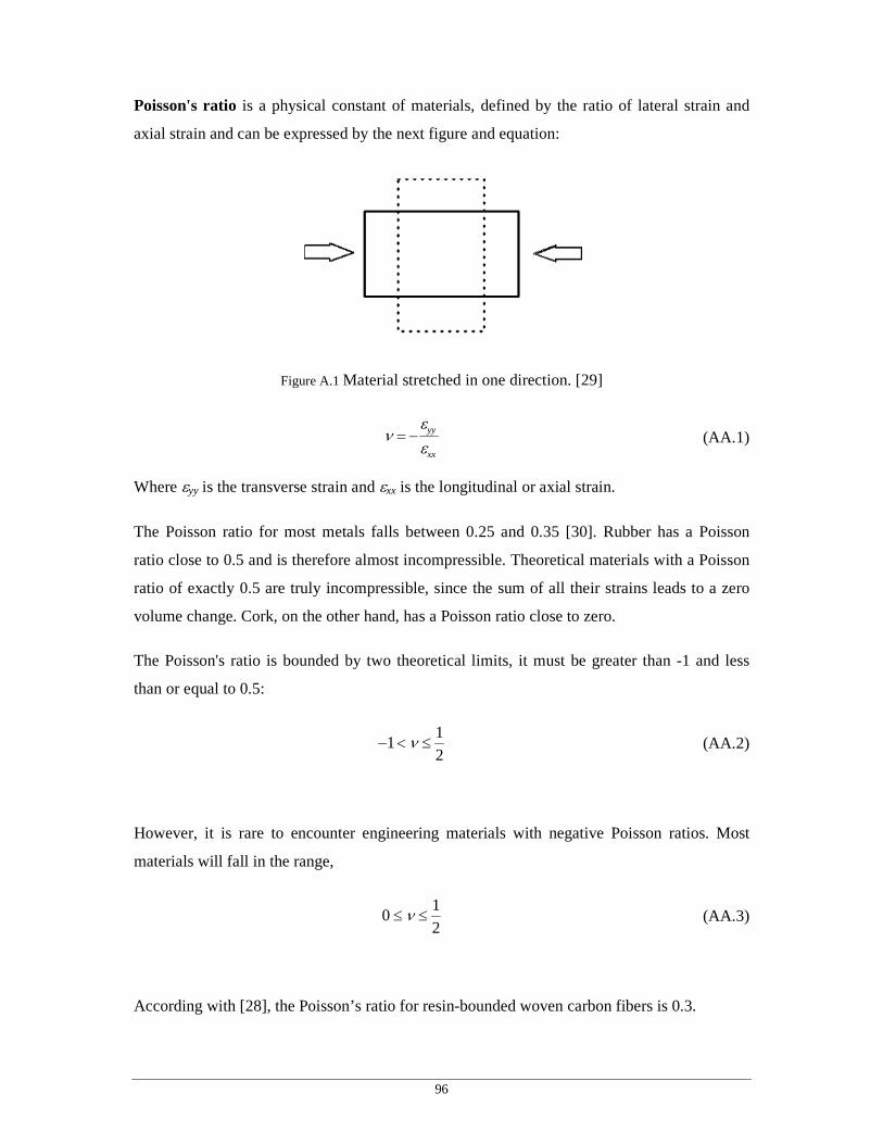
96

Poisson's ratio is a physical constant of materials, defined by the ratio of lateral strain and

axial strain and can be expressed by the next figure and equation:

Figure A.1 Material stretched in one direction. [29]

ν = −εyy

εxx

(AA.1)

Where εyy is the transverse strain and εxx is the longitudinal or axial strain.

The Poisson ratio for most metals falls between 0.25 and 0.35 [30]. Rubber has a Poisson

ratio close to 0.5 and is therefore almost incompressible. Theoretical materials with a Poisson

ratio of exactly 0.5 are truly incompressible, since the sum of all their strains leads to a zero

volume change. Cork, on the other hand, has a Poisson ratio close to zero.

The Poisson's ratio is bounded by two theoretical limits, it must be greater than -1 and less

than or equal to 0.5:

−1<ν ≤12

(AA.2)

However, it is rare to encounter engineering materials with negative Poisson ratios. Most

materials will fall in the range,

0≤ ν ≤12

(AA.3)

According with [28], the Poisson’s ratio for resin-bounded woven carbon fibers is 0.3.

97

Annex B

Calculations of a flywheel rotor’s

dimensions for different energy

capacities 7 Annex B - Calculations of a flywheel rotor’s

dimensions for different energy capacities

98

For the design of the flywheel, carbon AS4C was the chosen material, which density

isρ =1510Kg/m3.

The maximum tensile strength for this material is 1650 MPa. For the σt it will be used half of

the material’s maximum value, as a security factor.

σ t =1650

2MPa= 825MPa

For the inner and outer radius relation, ri

ro

=2

2 was achieved and for the height and outer

radius relation, h = 2⋅ ro was chosen (for size reasons).

ri

ro

= 22

⇒ ri

ro

4

= 14

h = 2⋅ ro

Using equation (2.13), the next simplification can be concluded:

Elim = 1

4⋅ π ⋅ h ⋅ 1− ri

ro

4

⋅ ro

2 ⋅σ t ⇒ Elim = 3

16⋅ π ⋅ h ⋅ ro

2 ⋅σ t ⇒ Elim = 3

8⋅ π ⋅ ro

3 ⋅σ t

For the linear speed and tensile strength relation, the next equation will be used:

σ t

ρ ⋅ω 2⋅ ro

2≈1

• 1st series of calculations (with σt=825MPa)

For this 1st series, the energy of the flywheel was fixed and the dimension and speed of the

wheel were calculated.

Calculation of rotor’s dimensions for Elim = 2.5kWh= 9MJ :

99

Elim =38⋅ π ⋅ ro

3 ⋅σ t ⇒ 9×106 =38⋅ π ⋅ ro

3 ⋅ 825×106 ⇒ ro = 0.21m

h = 2⋅ ro = 2×0.21= 0.42m

ri

ro

=2

2⇒ ri = 0.148m

Calculation of angular velocity for ro = 0.21m:

σ t

ρ ⋅ω 2 ⋅ ro2 =1⇒ω 2 =

825×106

1510×0.212 ⇒ω = 3519.95rad /s= 33613rpm

The calculation of rotors’ dimensions for Elim =1kWh= 3.6MJ and Elim = 25kWh= 90MJ

were made, using the same procedure as before, but with different values of energy. The

results can be seen in table 2.3.

• 2nd series of calculations (with σt=825MPa)

In this series, the maximum speed of the wheel was fixed and the wheel’s dimensions and

energy calculated.

Calculation of rotor’s dimensions for ω = 60000rpm= 6283.19rad /s

σ t

ρ ⋅ω 2 ⋅ ro2 =1⇒ ro

2 =825×106

1510×6283.192⇒ ro = 0.118m

h = 2⋅ ro = 2×0.118= 0.235m

ri

ro

=2

2⇒ ri = 0.083m

Calculation of the stored energy for ro = 0.118m:

Elim =3

8⋅ π ⋅ ro

3 ⋅σ t ⇒ Elim =3

8⋅ π ⋅ 0.1183 ⋅ 825×106 =1.58MJ = 0.441kWh

100

• 3rd series of calculations (with σt=825MPa)

These calculations intended to test safe limits. Certain energy and speed limits were specified,

being the size and the tensile strength calculated for the specified values.

Calculation of rotor’s dimensions forElim = 2.5kWh= 9MJ ; ω = 60000rpm=

= 6283.19rad /s:

σ t

ρ ⋅ω 2 ⋅ ro2=1⇔σ t = ρ ⋅ω 2 ⋅ ro

2

Elim = 1

4⋅ π ⋅ h ⋅ 1− ri

ro

4

⋅ ro

2 ⋅σ t ⇒ Elim = 1

4⋅ π ⋅ h ⋅ 1− ri

ro

4

⋅ ro

4 ⋅ ρ ⋅ω 2 = 3

16⋅ π ⋅ h ⋅ ro

4 ⋅ ρ ⋅ω 2

Elim =3

8⋅ π ⋅ ro

5 ⋅ ρ ⋅ω 2 ⇒ 9×106 =3

8⋅ π ⋅ ro

5 ⋅1510⋅ 6283.192 ⇒ ro = 0.167m

h = 2⋅ ro = 2×0.167= 0.333m

ri

ro

=2

2⇒ ri = 0.118m

Calculation of the tensile strength for ro = 0.167m:

σ t = ρ ⋅ω 2 ⋅ ro2 ⇒ σ t =1653.59MPa

This value is superior to the maximum admitted for the material.

The problem of this calculation is that the σt is not limited.

• 4th calculations (with σt=825MPa)

Supposing h = 4 ⋅ ro, instead of h = 2⋅ ro and using the method developed in the first

calculations, the calculation of rotor’s dimensions for Elim = 2.5kWh= 9MJ is:

101

Elim = 1

4⋅ π ⋅ h ⋅ 1− ri

ro

4

⋅ ro

2 ⋅σ t ⇒ Elim = 3

16⋅ π ⋅ h ⋅ ro

2 ⋅σ t ⇒ Elim = 3

4⋅ π ⋅ ro

3 ⋅σ t

Elim =34⋅ π ⋅ ro

3 ⋅σ t ⇒ 9×106 =34⋅ π ⋅ ro

3 ⋅ 825×106 ⇒ ro = 0.167m

h = 4 ⋅ ro = 4×0.167= 0.667m

ri

ro

=2

2⇒ ri = 0.118m

Calculation of angular velocity for ro = 0.167m:

σ t

ρ ⋅ω 2 ⋅ ro2 =1⇒ω 2 =

825×106

1510×0.1672 ⇒ω = 4434.85rad /s= 42350rpm

103

Annex C

FEMM and LUA script Annex C - FEMM and Lua script

Calculations of a flywheel rotor’s dimensions for different energy capacities In this annex a

brief description of the FEMM simulation program will be made, as such the LUA script also

used in this thesis

104

The Finite Elements Method Magnetics (“FEMM”), can be found in this url: http://femm.foster-miller.net/wiki/HomePage . This is a 2D simulation magnetic elements program.

The next figure shows the magnetic bearing studied in this thesis and implemented in the

program.

Figure C.1. FEMM with the magnetic bearing

In Figure A1.1, shows that only half of the bearing cross section was designed in the program.

After design the figure, a mesh has to be created. This mesh will help the program to calculate

the magnetic field values and flux paths.

The size of the mesh can be modified. It is important to take in mind that as smaller the mesh

become the more accurate is the value, but the program will take more time to converge. If the

mesh is so tiny, the program will probably will not converge.

105

Figure C.2. Magnetic bearing with the mesh already generated

After the mesh being generated the program is ready to calculate the magnetic field and the

lines of the magnetic field. The next figure shows the output of the program. It can be seen

the magnetic field lines and flux density is in the red and yellow areas the flux reaches the

higher values.

Figure C.3. Flux density output

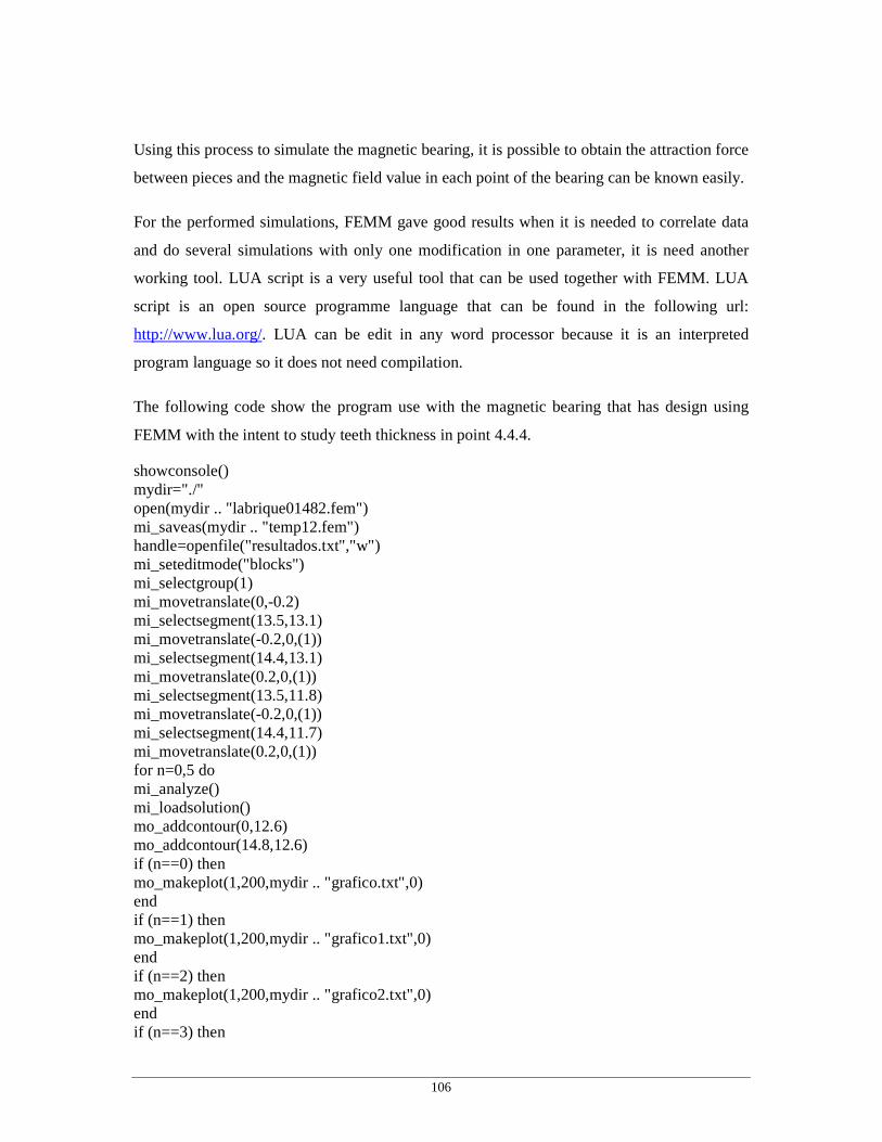
106

Using this process to simulate the magnetic bearing, it is possible to obtain the attraction force

between pieces and the magnetic field value in each point of the bearing can be known easily.

For the performed simulations, FEMM gave good results when it is needed to correlate data

and do several simulations with only one modification in one parameter, it is need another

working tool. LUA script is a very useful tool that can be used together with FEMM. LUA

script is an open source programme language that can be found in the following url:

http://www.lua.org/. LUA can be edit in any word processor because it is an interpreted

program language so it does not need compilation.

The following code show the program use with the magnetic bearing that has design using

FEMM with the intent to study teeth thickness in point 4.4.4.

showconsole() mydir="./" open(mydir .. "labrique01482.fem") mi_saveas(mydir .. "temp12.fem") handle=openfile("resultados.txt","w") mi_seteditmode("blocks") mi_selectgroup(1) mi_movetranslate(0,-0.2) mi_selectsegment(13.5,13.1) mi_movetranslate(-0.2,0,(1)) mi_selectsegment(14.4,13.1) mi_movetranslate(0.2,0,(1)) mi_selectsegment(13.5,11.8) mi_movetranslate(-0.2,0,(1)) mi_selectsegment(14.4,11.7) mi_movetranslate(0.2,0,(1)) for n=0,5 do mi_analyze() mi_loadsolution() mo_addcontour(0,12.6) mo_addcontour(14.8,12.6) if (n==0) then mo_makeplot(1,200,mydir .. "grafico.txt",0) end if (n==1) then mo_makeplot(1,200,mydir .. "grafico1.txt",0) end if (n==2) then mo_makeplot(1,200,mydir .. "grafico2.txt",0) end if (n==3) then

107

mo_makeplot(1,200,mydir .. "grafico3.txt",0) end if (n==4) then mo_makeplot(1,200,mydir .. "grafico4.txt",0) end if (n==5) then mo_makeplot(1,200,mydir .. "grafico5.txt",0) end mo_groupselectblock(1) mi_selectgroup(1) mi_movetranslate(0,0.1) fz=mo_blockintegral(19) print(fz) write(handle,"z=",0.6-(n)/10," ","FZ=",fz," Newton ","\n\n") end closefile(handle) For any doubt about FEMM and LUA script seen [23] and [24].

109

Annex D

Expressions of the electric

equivalent circuit 8 Annex D - Calculations of a flywheel rotor’s

dimensions for different energy capacities

110

Choosing the appropriate flux paths (3), it is possible to deduce an electric equivalent circuit

as it is shown in Figure D.1.

Figure D.1 Electric equivalent circuit of the active bearing

Furthermore, in order to study the complete circuit, the first step is to simplify the figure

AD.1 circuit (AD.2 circuit).

Figure D.2 Electric equivalent circuit of the active bearing simplified (Lα (Pm, g), Lβ(g))

From the analysis of the figure AD.2 circuit, the inductances depend on the permanent magnet

characteristics and of the air gap width. The electrical equation representing the circuit

behaviour is:

dt

dg

dg

dLI

dt

dILIru ⋅⋅+⋅+⋅= (AD.1)

Analysing the equivalent circuits (magnetic and electric), the expressions to Lα and Lβ can be

obtained.

111

Figure D.3 Magnetic equivalent of the active bearing with the flux path

Coming back to the magnetic equivalent circuit and defining the following flux paths, the

following equations are obtained:

( ) ( ) ( ) ( )( ) ( ) ( )( ) ( ) ( )

=ℜ+ℜ+ℜ⋅++ℜ+ℜ+ℜ⋅=ℜ+ℜ+ℜ⋅−+ℜ+ℜ+ℜ+ℜ⋅

=ℑ+ℜ+ℜ+ℜ⋅−ℜ+ℜ+ℜ⋅−+ℜ+ℜ+ℜ⋅

0

0

0

227262312171613

1312109212

217161313218541

gg

gmagnet

mggmagnet

φφφφφφ

φφφφ (AD.2)

The first equation can be expressed only as function of 1φ :

112

221227262217161

2272623

1111310921

132

φφφ

φφφ

⋅−=⋅ℜ+ℜ+ℜ+ℜ+ℜ+ℜ

ℜ+ℜ+ℜ−=

⋅=⋅ℜ+ℜ+ℜ+ℜ+ℜ+ℜ+ℜ

ℜ+ℜ+ℜ=

k

k

gg

g

gmagnet

gmagnet

(AD.3)

So:

( )( ) 0

2171612

131354

1 =+

ℜ+ℜ+ℜ++ℜ+ℜ+ℜ−ℜ+ℜ+ℜ+ℜ+ℜ⋅ NI

k

k

g

gmagnetgmagnetφ (AD.4)

Which is equivalent to:

02

211 =+ℜ⋅+ℜ⋅−ℜ

⋅⋅dt

dI

N

kk

dt

dN γψϕφ (AD.5)

In addition, taking the time derivative of the equation above:

02

211 =+ℜ⋅+ℜ⋅−ℜ

⋅⋅dt

dI

N

kk

dt

dN γψϕφ (AD.6)

Introducing the following electrical variables in previous equation above:

dt

dNv 1

1

φ⋅=

(AD.7)

and:

113

,1

2

21

1 N

kk

Lγψϕ ℜ⋅+ℜ⋅−ℜ

= (AD.8)

it is possible to express the electrical equation representing the circuit behaviour as function

of the magnetic reluctances:

dt

dg

dg

dLI

dt

dI

kk

NIru

dt

dg

dg

dLI

dt

dILIru

⋅⋅+⋅ℜ⋅+ℜ⋅−ℜ

+⋅=⇒

⇒⋅⋅+⋅+⋅=

11

1

21

2

111

11

11111

γψϕ

(AD.9)

Coming back to the figure 1 and 2 circuits, it is possible to represent the magnetic circuit in

the following simple form:

Figure D.4 Simplify magnet equivalent circuit

Where:

114

( ) ( )1310921

1310921

gmagnet

gmagnet

ℜ+ℜ+ℜ+ℜ+ℜ+ℜ+ℜℜ+ℜ+ℜ⋅ℜ+ℜ+ℜ+ℜ

=ℜα (AD.10)

And:

( )227262217161

227262217161854

)(

gg

gg

rrrr ℜ+++ℜ++ℜ+ℜ+ℜ⋅ℜ+ℜ+ℜ

+ℜ+ℜ+ℜ=ℜβ (AD.11)

So:

( ) 002

=+

ℜ+ℜ⋅⋅⇒=⋅+ℜ+ℜ⋅

dt

dI

Ndt

dNIN αβ

αβ

βααβαβαβαββααβ

φφ (AD.12)

From the above equations, the following relationship can be obtained:

( ) ( )( ) ( )( ) ( )227262217161

227262217161854

22726221716122

1310921

131092122

gg

gg

gg

gmg

gmagnet

NN

L

NN

L

ℜ+ℜ+ℜ⋅ℜ+ℜ+ℜ++ℜ+ℜ+ℜ+ℜ+ℜ+ℜ⋅ℜ+ℜ+ℜ

ℜ+ℜ+ℜ+ℜ+ℜ+ℜ⋅=

ℜ=

ℜ+ℜ+ℜ⋅ℜ+ℜ+ℜ+ℜℜ+ℜ+ℜ+ℜ+ℜ+ℜ+ℜ

=ℜ

=

αββ

αββ

αβα

αβα

(AD.13)

The electrical equation representing the system behaviour is now:

dt

dg

LL

LL

dg

dI

dt

dI

LL

LLIrv ⋅

+⋅⋅⋅+⋅+

⋅+⋅=βα

βααβ

αβ

βα

βααβαβαβ (AD.14)

115

And where βα

βαLL

LL

dg

d

+⋅

⋅ is:

( ) ( ) ( ) ( )( )

( ) ( ) ( ) ( ) ( )( ) =+

⋅⋅+−+⋅

⋅+

=

=+⋅⋅+−+⋅⋅

=

+⋅⋅

2

2

βα

βαβαβαβαβα

βα

βαβαβαβα

βα

βα

LL

LLLLdg

dLLL

dg

dLLL

dg

d

LL

LLLLdg

dLLLL

dg

d

LL

LL

dg

d

(AD.15)

116

( )

( ) ( )( )

( )( )

( )

( ) ( ) ( )( )( )( )

( ) ( )

( )

−⋅⋅+

⋅

−⋅+++−⋅++

−⋅

+−⋅

⋅

−⋅

++

−

−⋅+++−⋅++⋅−⋅

+

+

−⋅⋅+⋅

⋅

−⋅++++++

−⋅⋅

⋅

−⋅++

−

−⋅++++++⋅−⋅

−−⋅=

⋅+⋅+

⋅+⋅−=

23

240

2

2

25

260

726223

240

7161

25

260

23

240

25

260

7262

25

260

726223

240

716125

260

21

220

1

2

21

220

310921

21

220

21

220

3

21

220

31092121

220

21

220

22

111

1

1

11

1

1

1

1

rrkr

rr

grr

rr

grr

rr

rr

rr

g

rr

rr

grr

rr

grr

rr

rrkr

rr

grrrrrr

rr

rr

grr

rr

grrrrrr

rr

rr

dg

drkr

dg

dk

dg

drkr

dg

dk

dg

dr

dg

dL

mag

mag

mag

πµ

πµπµ

πµ

πµ

πµ

πµπµπµ

πµ

πµ

πµ

πµ

πµπµ

πµ

γ

ψ

γγ

ψψ

ϕ

(AD.16)

117

( ) ( ) ( ) ( )( ) ( )

( ) ( )

−⋅++⋅+++

−⋅++++++⋅+++⋅

⋅−⋅−

−⋅+++++⋅−⋅

=2

21

220

310921

21

220

31092110921

21

220

21

220

31092121

220

2

11

rr

grrrrrr

rr

grrrrrrrrrr

rrrr

grrrrrr

rr

NLdg

d

mg

mg

mg

πµ

πµ

πµπµπµ

αβα (AD.17)

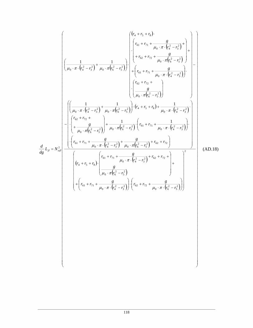
118

( ) ( )

( )( )( )( )

( )( ) ( ) ( ) ( )

( ) ( ) ( )

( ) ( )

( ) ( )( )( ) ( )

−⋅⋅++⋅

−⋅⋅+++

+

−⋅

+++−⋅⋅++⋅++

++−⋅+−⋅⋅++⋅

⋅

−⋅⋅++⋅−⋅+

−⋅+++

⋅

⋅−⋅⋅+++⋅

−⋅+−⋅⋅

−

−

−⋅

++⋅

⋅

−⋅⋅+++

+

−⋅+++

+−⋅⋅++⋅

⋅++

⋅

−⋅+−⋅⋅

=2

25

260

726223

240

7161

25

260

726223

240

7161

854

726225

260

23

240

7161

23

240

716125

2602

52

60

7262

23

240

85425

260

23

240

25

260

7262

23

240

7161

25

260

7262

23

240

7161

854

25

260

23

240

2

11

111

11

rr

grr

rr

grr

rr

g

rrrr

grr

rrr

rrrr

g

rr

grr

rrrr

rrrr

g

rr

rrrrr

rrrr

rr

g

rr

rr

grr

rr

grr

rr

grr

rrr

rrrr

NLdg

d

πµπµ

πµ

πµ

πµπµ

πµπµπµ

πµπµπµ

πµ

πµ

πµ

πµ

πµπµ

αββ

(AD.18)

121

References

References [1] Hoolboom, Gerard J.; Szabados, Bama; “Nonpolluting Automobiles”, IEEE

Transactions on Vehicular Technology, vol. 43, no. 4, pp 1136-1144, November

1994.

[2] Kenny, Barbara H.; Jansen, Ralph; Kaskak, Peter; Dever, Timothy; Santiago,

Walter; “Integrated Power and Attitude Control with Two Flywheels”, IEEE Log

No. T-AES/41/4/860803, April 2005.

[3] Strasik, M.; Johnson, P. E.; Day, A. C.; Mittleider, J.; Higgins, M. D.; Edwards,

J.; Schindler, J. R.; McCrary, K. E.; McIver, C. R.; Carlson, D.; Gonder, J. F.;

Hull, J. R.; “Design, Fabrication, and Test of a 5-kWh/100-kW Flywheel Energy

Storage Utilizing a High-Temperature Superconducting Bearing”, IEEE Trans.

Appl. Supercond., vol. 17, no. 2, pp 2133–2137, June 2007.

[4] Werfel, Frank N.; Floegel-Delor, Uta; Riedel, Thomas; Rothfeld, Rolf; Wippich,

Dieter; Goebel, Bernd; Reiner, Gerhard; Wehlau, Niels; “A Compact HTS 5

kWh/250 kW Flywheel Energy Storage System”, IEEE Trans. Appl. Supercond..

[5] Bolund, Bjorn; Bernhoff, Hans; Leijon, Mats; “Flywheel Energy and Power

Storage Systems”, Renewable and Sustainable Energy Reviews 11, pp 235–258,

2007.

[6] Schweitzer, G.; “Active Magnetic Bearings – Chances and Limitations”,

International Center for Magnetic Bearings, ETH Zurich, CH–8092 Zurich.

[7] Schouler, Adrien; Sapin, Julien; Kluyskens, Virginie; Labrique, Francis; Dehez,

Bruno; “Study and control of magnetic bearing for flywheel energy storage

system, Setubal, 2007.

[8] Xia, Z.; Chen, Q. Y.; Ma, K. B.; McMichael, C. K.; Lambs, M.; Looley, R. S.;

Fowler, P. C.; Chu, W. K.; “Design of superconducting Magnetic Bearing with

122

High Levitations Forces for Flywheel Energy Storage System”, Texas, 1995.

[9] Teshima, Hdekazu,; “Ring Shaped Flywheel Energy Storage systems with

superconducting levitation”, Japan.

[10] Iori, T.; Ogawa, S.; Sugiura, T.; “Nonlinear effects of electromagnetics forces on

primary resonance of a levitated elastic bar supported by high-Tc superconducting

bearing”, Kelo University, 3-14-1 Hiyoshi, Kohoku-Ku, Yokohama, Kanagawa,

223-8522, Japan, 2007.

[11] Chu, G. G.; Silva Neto, J. C. da; Andrade Jr. R. de; Ferreira A. C.; Nicolsky, R.; “

Comparative analysis of two topologies for rotational superconducting magnetic

bearing”, Rio de Janeiro, Brazil, 2007.

[12] Kirby, Brendan; “Frequency Regulation Basics and Trends”, Oak Ridge National

Laboratory, 2004.

[13] Kenny, Barbara H.; Kascak, Peter E.; Jansen, Ralf; Dever, Timothy; “A flywheel

Energy Storage System demonstrations for space applications”, 2003.

[14] McLallin, Kerry, “NASA Flywheel System Development”, Space Power

Workshop, 2001.

[15] Rojas, Alex, “WindPower 2003, Integrating Flywheel Energy Storage System in

Power Applications”, Beacon Power Corp., 2003.

[16] Fausz, Jerry L., “AFRL/NASA Flywheel Program Overview”, Glenn Research

Center, 2002.

[17] Hillyard, Jeef, “Magnetic Bearings”, Technische Universität München, 2006.

[18] Bolund, Björn; Bernhoff, Hans; Leijon Mats; “Flywheel energy and power storage

systems”, Sweden, 2005.

[19] Yanlians, Xu; Yueqin Dun; Xiuhe Wang; Yu, Kong; “Analysis of Hibrid

Magnetic Bearing with permanent Magnet in the Rotor by FEM”, IEEE

Transactions on Magnetics, Vol. 42, NO. 4, April, 2006 .

[20] Lazarewicz, Matt, “A Description of the Beacon Power high energy and high

123

power composite flywheel energy storage system”, Beacon Power Corp.

[21] Fitzgerald, A. E.; Kingsley Jr., Charles; D. Umans Stephen; Electric Machinery”

6th Edition, McGraw-Hill Higher Education, 2003

[22] Jufer, M.; “Electromecanique”, PPUR, Lausanne,1995.

[23] Meeker, Davis “Finit Element Method Magnetics Version 4.2 User’s Manual”,

http://femm.foster-miller.net/Archives/doc/manual42.pdf, 2007.

[24] Lerusalmschy, R.; Figueiredo L. H. de; Celes, W.; “LUA 5.1 Reference Manual”,

ISBN – 85-903798-3-3.

[25] MS-196. Project all electric vehicle (AEV). RTP 16.02 inom WEAG. Technical

Report No. 1; Nov–Dec 2001.

[26] Cimuca, Gabriel–Octavian; “Systeme Inertiel de Stockage d’Energie Associe a

des Generateurs Eoliens”,Ph.D. thesis, Ecole Nationale Supérieur d’Arts et

Métiers, Centre de Lille, France, 2005.

[27] Taylor, P.; Johnsson, L.; Reichert, K.; DiPietro, P.; Philip, J.; Butler, P.; “A

summary of the state of the art of superconducting magnetic energy storage

systems, flywheel energy storage systems and compressed air energy storage

systems”, SAND99-1854, unlimited release; Albuquerque, New Mexico 87185

and Livermore, California 94550: Sandia National Laboratory; 1999.

[28] Marques, M. I. L.; “Design and Control of an Electrical Machine for Flywheel

Energy-Storage System”, M.A. thesis, IST, Lisbon, Portugal, June 2008.

[29] http://www.engineeringtoolbox.com/poissons-ratio-d_1224.

[30] Budynas, Richard G.; Nisbett, J. Keith; “Shigley’s Mechanical Engineering

Design”, Eight Edition, ISBN 978-007-125763-3, McGraw–Hill, October 25,

2006.

Preliminary Approach Designing an Electromagnetic … Approach Designing an Electromagnetic Bearing...

Documents

Transcript of Preliminary Approach Designing an Electromagnetic … Approach Designing an Electromagnetic Bearing...