Preface - The University of Western Web viewexperiment on intrinsic motivation and extrinsic...

1

Crowding in or crowding out? A laboratory

experiment on intrinsic motivation and extrinsic incentives

Zack Dorner∗1 and Emily Lancsar2

1Department of Economics, Monash University2Centre for Health Economics, Monash

University September 26, 2016

AbstractThis paper uses a laboratory experiment to investigate

the extent to which intrinsic motivation can be crowded in or out by adding and then removing monetary or non-monetary incentives. The impact of size and type of incentive on motivation is tested between subjects. Furthermore, we investigate whether this effect is homogeneous or heterogeneous depending on baseline intrinsic motivation to address a gap in the literature. The analysis includes survey data on participants’ pro-environmental and health behaviours, along with physically measured body mass index and waist size. The findings of the project may be useful for informing health and environmental policy.

∗Corresponding author: [email protected] Gangadharan in particular is acknowledged for the extensive supervision given throughout this project. A thank you also for the

2

supervision provided by Anke Leroux and Paul Raschky.Funding for this project is from the Australian Research Council (ARC), through a Discovery Early Career Researcher Award (DECRA) (Grant ID DE140101260). This project has been approved by the Monash University Human Research Ethics Committee; MUHREC#: CF16/618 - 2016000300.

3

PrefaceThesis title: Three Essays in Environmental EconomicsSupervisors: Professor Lata Gangadharan, Associate Professor Paul Raschky and Dr Anke Leroux.

Within the broader field of environmental economics, the chapters in my thesis look at how preferences - in particular risk preferences, social preferences and intrinsic motivation - drive decisions and behaviour. These preferences are identified using experimental methods, both in the field and the lab, with a key element of interest being heterogeneity. A further theme is technological change, in terms preferences over utilis- ing new technologies, and how technological change might influence pro-environmental behaviours through a behavioural rebound effect. Finally, as in the paper presented here, the thesis investigates the impact of incentives - monetary and non-monetary - on behaviour change. Along with an introduction and conclusion, the thesis will have three main chapters. They are as follows:

1. Preferences for Intrinsically Risky Attributes – with Daniel Brent and Anke Ler- oux (Monash Business School Department of Economics Discussion Paper 32/16).In this chapter, we develop a novel approach to leverage data on risk preferences from a fully incentivized risk elicitation task to model intrinsic riskiness of alter- natives in a choice experiment. In a door-to-door survey, 981 respondents partici- pated in a discrete choice experiment (DCE) to elicit preferences over alternative sources of municipal water, conditional on water price and quality. Participants were not given information about supply or technological risks of the sources to avoid framing effects driving the results. Controlling for water quality and cost, we find that supply risk is an important determinant of participants’ choices, while respondents are not concerned about technology risk.

2. Crowding in or Crowding Out? A laboratory experiment on intrinsic motivation and extrinsic incentives – with Emily Lancsar (presented in this document).

3. Laboratory Experiment Investigating the Behavioural Rebound Effect.The focus of the third chapter will be investigating the environmental rebound effect in a laboratory setting, in order to better understand some of the behavioural drivers. Evidence around the rebound effect and its size to date is primarily from secondary field data, such as household energy usage and household production technology change, and most studies are not designed to identify behavioural drivers (Gillingham et al., 2016; Sorrell et al., 2009). The laboratory setting allows particular aspects of the rebound effect to be isolated; in this case the be-

4

havioural impact of exogenous versus endogenous technological change and the importance of the baseline environmental impact of consumption.

5

1 IntroductionEvidence on the potential for extrinsic incentives to reduce intrinsic motivation motivation has been gathering since Deci’s seminal article in the field of psychology (Deci, 1971). The counter-intuitive notion that external incentives, especially monetary incentives, could lead to the crowding out of effort is now widely accepted in economics too (Frey, 1997; Frey and Jegen, 2001; Gneezy et al., 2011). With crowding out, one or both of the following occurs: effort is reduced after the application of incentives or effort is reduced below pre-incentive levels after the removal of temporary incentives. Intrinsic motivation to do an activity can take many forms, such as the enjoyment of a particular activity, the desire to engage in productive and meaningful work, the benefits to one’s self image from undertaking an activity and prosocial motivation (Promberger and Marteau, 2013). Take exercise as an example. Generally individuals must find some way of motivating themselve to exercise, rather than rely on exernal incentives. One person may enjoy exercise, someone else might motivate themselves by striving to be a fit, healthy and attractive person. Another person may motivate themselves by wanting to stay healthy so that they can be around for their family as long as possible. Crowing out theory notes the possibility that paying someone to exercise could lead to this external incentive dominating the motivation for exercise and leading to an overall reduction in the level of exercise undertaken after payments start. If the incentive is large enough, the level of exercise may increase. However, when the incentive is removed, if crowding out has occurred then the level of exercise may drop below is original pre-incentive level. The possibility of crowding in also exists – after payment ceases, exercise may remain at a higher level than before.

As noted in this example, there are a range of types of intrinsic motivations someone might use to exercise. Naturally, there is great heterogeneity in the level of exercise undertaken by heterogeneous individuals. This fact leads to several questions. What are some of the factors that determine intrinsic motivation? And, how might external incentives affect a person with low intrinsic motivation compared with someone with a high level of intrinsic motivation?

In this paper we aim to address these questions. In a laboratory setting we give a real effort task to a heterogeneous, non-undergraduate student participant pool. We give the task to the participants for one round, with no incentives or mention of future

6

incentives. In a second round, the participants are given the task again, with all but the control group given some sort of incentive (which vary by size and type). In the third round, the incentive is removed. A fourth round, again without incentives, is also given to participants, after a break in which another task is completed. Thus, we have a measure of baseline intrinsic motivation (round 1), test the effects of a range of incentives (round 2) and test the ongoing effect of removing those incentives (rounds 3

7

and 4). We also measure health and environmental variables related to the participants, which provide useful applications for the study results. We find the low power incentive is the only incentive effective at increasing effort in round 2, whereas the high power incentives only serve to crowd out effort in the subsequent rounds, particularly amongst those with the highest levels of original intrinsic motivation.

The crowding out effect can be identified when raising incentives decreases rather than increases supply of effort. Under the motivation crowding model, a small monetary incentive may lead to a decrease in supply, due to the crowding out effect dominating the positive effect of the incentive. An increase in supply can be garnered, provided there is a large enough external incentive provided. If this crowding out effect has operated through changed preferences, changed information (on the side of the agent about the principle’s motivations), lowering self agency or lowering the enjoyment of the task, the crowding out effect will persist after the incentive is removed (Frey and Jegen, 2001; Gneezy and Rustichini, 2000a,b). A large portion of the economic literature has focussed particularly on prosocial motivation and potential crowding out effects in this area (Promberger and Marteau, 2013). More recent theoretical models emphasise the roles of image motivation (both self- and public image) and core beliefs as assets to explain prosocial behaviours and cases of crowding out (B´enabou and Tirole, 2006, 2011). Conversely, the emphasis of intrinsic motivation literature in psychology has been motivation to do enjoyable activities – activities which are done for their own sake (Deci et al., 1999; Promberger and Marteau, 2013). This focus is not without contention. Cameron et al. (2001) argue that intrinsic motivation should be approached with a more broach definition. Given this broad definition, the literature shows that crowding out is not pervasive, but applicable only to high interest tasks with tangible rewards that are at least loosely performance-based.1

The laboratory setting has provided important insights into intrinsic motivation and crowding out. Indeed, of the three experiments conducted by (Deci, 1971), two of them are laboratory experiments. Particularly for the within-subject component of our experimental design, we build on the basic structure of Deci’s laboratory experiments. He measures baseline intrinsic motivation in the first round of a puzzle task, gives a monetary or non-monetary (verbal affirmation) incentive in a second round and then removes the incentive in the third round. There is also a control group with no incentive. The monetary

8

incentive is found to crowd out intrinsic motivation (Deci’s experiment 1) and the verbal affirmation crowds in intrinsic motivation (Deci’s experiment 3). Ma et al. (2014) present a recent laboratory study with the same three round design showing that crowding out effect of a monetary incentive operates at a neuro- logical level. To the best of our knowledge, there is a gap in the literature in terms of testing a range of incentive types, which is covered in this paper by the between sub-

1For the response to Cameron et al. (2001), see Deci et al. (2001).

9

ject aspect of our experimental design. There is a further gap in terms of investigating heterogeneous responses to such a 3 round laboratory design. Finally, our study adds a fourth round to test persistence.

Our study has a generic laboratory design, using a real effort task without any further framing for participants. Given the importance of context within the intrinsic motivation literature, we further collect data on two contexts for which intrinsic motivation is important. The health context is of interest given the private nature of benefits to exercise – that is, greater health, plus enjoyment from exercise for some individuals. Health has the added advantage of having a variable that is observable in a laboratory setting - namely weight. The environmental context is a useful example of a context where intrinsic motivation is of a pro-social nature. The advantage of the environmental context for this study is that pro-environmental preferences are perhaps more heterogeneous than other contexts; mitigating climate change is a much more controversial pursuit than feeding people who lack sufficient access to food.

This paper is organised as follows. The second section below outlines the methodol- ogy, including research questions, a description of the experiment and how the sample was recruited. The results are presented in Section 3, while Section 4 provides a discussion and conclusion.

2 MethodGiven the general questions and strands of literature identified in the introduction, this paper specifically seeks to address the following main research questions: First, what factors help explain initial level of intrinsic motivation? Second, how does level and type of incentive impact effort? Third, to what extent does level and type of extrinsic incentive crowd in or crowd out intrinsic motivation? Fourth, how does heterogeneity in level of intrinsic motivation impact the efficacy of incentives and the level of crowding in or out of incentives? Fifth, is level of intrinsic motivation and crowding in or out observed in a general lab context consistent with self reported attitudes and behaviours in the field; in particular health and environmental attitudes and healthy and pro- environmental behaviours? Our method is to utilise a generic laboratory setting, which is described in this section.

10

2.1 Experimental designThe experiment was run over 12 sessions from 6 April to 3 June, 2016, at the Monash Laboratory for Experimental Economics (MonLEE) at Monash University in Mel- bourne, Australia. The overall timeline of each experimental session is shown in Table 1.

11

Table 1: Overall timeline of each experimental session.

Initialisation Activities Surveys Measurementand payment

Participants ran- Activities for the Surveys on health,

Participants in-domly assigned to

experiment com- the structed to proceedcomputers, con- pleted –

multipleactivities and the

to aneighbour-sent forms

signed,rounds of

effortenvironment given

ing room to beoverview task and a time to participants. measured andtions provided in preferences task paid in private

byhard copy and (see Table 2 for assistants.read aloud by more detail).experimenter.

At the start of each session, each participant took a random number from a bucket, which corresponded to one of the 26 computers in the room. They were seated, signed consent forms and then overview instructions were provided in hard copy and read aloud. The instructions outlined the overall session structure, without giving detail about the activities themselves. At this stage it was explained to participants that they would be paid at the end of the activity by an administrative assistant in a neighbouring room. Next, the activities were undertaken, followed by surveys on health, the experimental activities and the environment. These tasks were all undertaken on the computers. When the participant was finished these activities, they were asked to line up outside the neighbouring room where they would be weighed, have their height and waist measured, and be paid.

The activities section of the experiment proceeded as shown in Table 2. We employed multiple rounds of a real effort task in order to address the research questions. We used the word encoding real effort task developed by Erkal et al. (2011), pro- grammed using zTree (Fischbacher, 2007). The number pad on the right-hand side of the keyboard, along with the tab keys were disabled for all participants in all sessions to remove the advantage a particularly experienced computer user could have in the task.

In the activities portion of the session, first the word encoding task was explained and a 2 minute practice round was given to participants. An example screenshot of the task is shown in Figure 1. The task consists of correctly inputting numbers in the boxes below the 5 randomly selected letters. Once the numbers are correctly inputted and the participant clicks “OK”, they are given a new random “word” and set of code numbers for the alphabet. The outcome variable measured

12

from the task is effort in terms of words completed per minute.After the first round, participants were told that they would be given

the same task again, for another 5 minutes. Those in the control group were given the task as before,

Table 2: Experimental activities timeline.

Between sub-ject

treatment

Practice round Round 1 Round 2 Round 3 Time

prefer-ences task

Round 4

Control group Effort task ex-plained and practice round given.

Effort task withno incentives; no incentives or future rounds mentioned.



Time preferencestask explained and given; next effort task round not mentioned.

Effort task withno incentives;no incentives mentioned nor that this is the Extrinsic

in-centive groups (four separate groups, each with a different type of incentive)

Effort task ex-plained and practice round given.


Effort task withextrinsic in-centive

(type depending on treatment group); no

Effort task withno incentives; made clear that no incentivesare given in this round, no future rounds

Time preferencestask explained and given; next effort task round not mentioned.

Effort task withno incentives; made clear that no incentives are given in this round, not mentioned Task time

limit2 minutes 5 minutes 5 minutes 5 minutes No time limit 5 minutes

7

8

Figure 1: Example screen of real effort task given to participants, with the code for the first letter of the “word” completed.

without mention of incentives or future rounds of the task. However, participants in the extrinsic incentive treatment groups were given an incentive to complete each word in the task during this round. The incentive given depended on the between subject treatment group – see Section 2.1.1. Like the control group, the participants in the incentive groups were not told about future rounds at this stage either. Therefore, round 2 gives a measure of the effect of the incentives, given baseline intrinsic motivation measured in the practice round and round 1.

After round 2, participants proceeded to round 3, which was the real effort task for another 5 minutes. There were no incentives given in this round; participants in the incentive groups were told this explicitly, whereas those in the control group were again just given the task without mention of incentives. This round gives a measure of whether the incentives crowd in or crowd out intrinsic motivation, given baseline intrinsic motivation measured in the practice round and round 1.

Next the participants were given a time preferences task, which is explained in more detail in Section 2.1.2. This task was given to participants at this point to give them a break from the real effort task to test whether the patterns measured in round 3 persisted after a

8

break. Thus, after the time preferences task participants were given the effort task in round 4 for another 5 minutes, with the same treatment as round3. That is, no incentives were given, which was explained to those in the incentive treatments but not mentioned to those in the control. It was not mentioned that this was the last round of the effort task.

9

Payment was received for round 2 (depending on treatment and number of words completed), the time preferences task (between AUD$10 and AUD$20), and AUD$20 for participating in a survey and discrete choice experiment on health during the survey component of the session. This means participants earned at least AUD$30 for participating in the session. Payments for the time preference task were made using a gift card (explained more in Section 2.1.2); all other payments were in cash. Given the time required for measurement and payment at the end, participants were instructed to leave the computer lab and line up outside the neighbouring room once they finished the surveys. This arrangement meant the fastest participants were paid and able to leave after just over an hour, and the last participant left after around 1 hour and 45 minutes.

Consideration was taken in the experimental design to minimise experimenter demand, so that the effort given in the practice rounds and round 1 constitute a good measure of intrinsic motivation rather than being explained by experimenter demand. The following was included in the overview portion of the instructions at the start of the experiment:

An administrative assistant will be paying you at the end of the laboratory session in the neighbouring room. He or she will not be involved in analysing the data from this experiment. I will record the payment details for each ID number and hand this to an administrative assistant. At the end of the session you will be instructed to take the ID number on your desk, and hand this to an administrative assistant, who will organise your payment.

Furthermore, the instructions for the real effort task were carefully worded to avoid telling participants to maximise the number of words they completed per minute. Words like “should” and “must” were avoided. Regarding the completion of words, the instructions before the practice round state:

In order to encode the word you can click on each box with your mouse and type the number associated with each letter. ... After you have completed a word it will be counted if you click OK with your mouse. The OK button is located at the bottom of the screen. If you click OK you will be given a new word to encode. The computer will not give you a new word until the word you have encoded is correct.

These instructions were kept constant between all sessions so that any experimenter demand effects will be the same between participants.

2.1.1 Between subject treatments

1

The 5 between subject treatment groups are shown in Table 3. Each session was assigned into one of the treatments. The treatments are defined by the extrinsic incentive applied in round 2 of the activity. As explained in the previous subsection, the control group received no incentive in round 2. The first of the incentive treatments is low

1

Table 3: Between subject treatment groups.

Treatment group Incentive applied (in Round 2 only)Control NoneLow power $0.05 paid per wordHigh power $1 paid per wordHigh power threshold

$23 paid if complete 23 words; $1 paid per word above thisamount

Charity 2 words plants one indigenous tree within Victoria (equiva-lent to $1 per word)

power; participants received AUD$0.05 for each 5 letter “word” completed during the 5 minute time limit of round 2. The high power treatment group received AUD$1 per word in round 2. Those participants in the high power threshold treatment received AUD$23 if they completed 23 words; below 23 words they received nothing, but for each word completed above 23 they received AUD$1.

Finally, participants in the charity treatment were told “every 2 words you complete will fund the planting of one indigenous tree in Victoria. A local environmental charity will receive the funds to plant these trees after the experiment.” The charity to which the funds were given, Tree Project, quotes on their website that every AUD$2 donated leads to one tree being planted.2 Thus, while participants were not told the monetary amount of their donation until the end of the experiment, it is equivalent to AUD$1 per word completed. The difference from the high power treatment is that donations were done in $2 increments. To ensure credibility of donations, participants were also told before round 2 started that a session-level donation receipt would be emailed to them to prove the donation had been made, which would include the average number of trees planted per person.

2.1.2 Time preferences task

The time preferences task consisted of 18 questions as shown in Table 4. The nine questions were repeated for today versus 5 weeks, and 5 weeks versus 10 weeks. This design means we can determine whether the participant is present or future bias, along with giving us a measure of how impatient the participants are.

It was explained at the start of the task that one question would be randomly selected to be paid out. The payments for this task were made using a WISH gift card, which can be used at one of the common supermarket chains, a major department store chain and a range of

1

other chain stores. The gift card was chosen as it can be used at a large number of stores where people commonly shop, and can be sent via the post. It does not have the transaction costs of going to a bank to deposit a cheque.

2http://www.treeproject.org.au/, accessed 23 August, 2016.

1

Table 4: Options given in time preferences task questions – for today and 5 weeks, and 5 weeks and 10 weeks.

Earlier payment Payment 5weeks

later$10 $10.05$10 $10.10$10 $10.50$10 $11$10 $12$10 $13$10 $15$10 $17$10 $20

2.2 SampleThe sample consists of individuals who are not undergraduate students, who could travel to Monash University Clayton Campus for one of the experimental sessions. Participants were recruited from Monash University’s Centre for Health Economics Database and through other advertisements, including on the Gumtree website (Vol- unteers Section), the Monash University staff newsletter and the local community news- paper The Leader.

Sessions were held on weekdays, at either 12pm or 5:30pm. In order to avoid differences in the composition of the treatment groups, each treatment was assigned to one 12pm session and one 5:30pm session. The aim was to have 50 people in each treatment group. However, the number of no shows in each session had a high variance, meaning it was difficult to reach the required number of participants in each session. Thus, two smaller extra sessions were run at 12pm for the control and the high power threshold treatments to supplement the numbers in those treatments.

3 Results

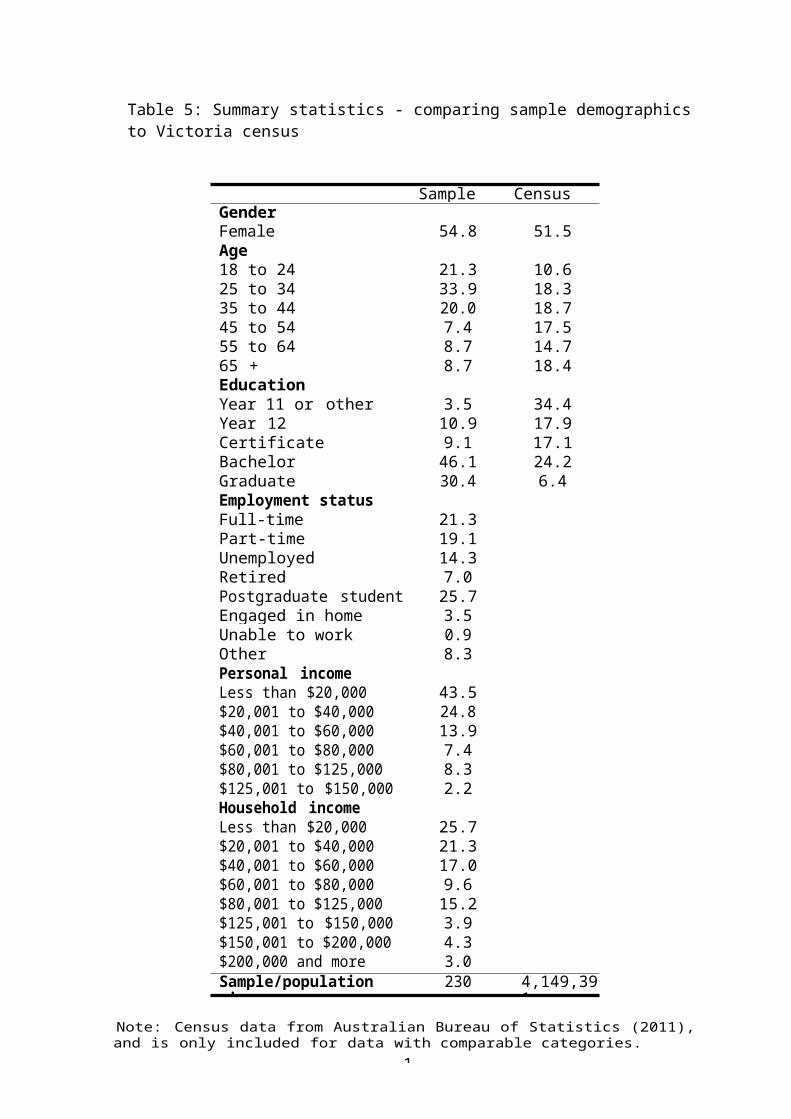
3.1 Summary statisticsTable 5 summarises the main demographic variables collected on the study participants, comparing some categories to the 2011 census data for Victoria. This is the appropriate population of comparison as, according to postcode data collected in the study, some participants are from parts of Victoria outside of greater Melbourne, even though the

1

study was conducted within Melbourne. We do not make any claims of representativeness, but as treatments were randomly assigned we did aim to ensure participants were similar accross the treatment groups. We can also control for the

1

Figure 2: Time preference choices - proportion choosing higher future payment, over an earlier payment of $10.

demographic variables in the study analysis. We aimed to have a range of individuals sampled in order to ensure heterogeneity of the subject pool. The subject pool is mostly non-students (74%) and exclusively non-undergraduate students to increase the external validity of the results. Overall, the sample is younger and better educated compared with the census data.

The raw time preference data is shown in Figure 2. It shows the proportion of participants choosing the higher future payment, according to the value of that payment. Both the today versus 5 week and 5 week versus 10 week payment choices are shown. While they track each other closely in aggregate, many participants had different switch-points in the two sets of questions. A different switch-point in the two sets of questions indicates whether the participant is present-biased or future-biased. For example, consider a participant who switches from choosing the earlier payment to the later payment at the $12 mark for today versus 5 weeks, and switches to choosing the later payment at the $11 mark for 5 weeks versus 10 weeks. She will be considered present biased. The opposite case is someone who is future biased. Of the 230 participants, 22% show present bias and 28% show future bias.

Table 6 shows summary statistics of the health and environmental

1

variables collected on participants. Height, weight, waist and BMI are shown by gender. A healthy BMI is considered to be between 18.5 and 25; thus on average females in our sample are slightly below the threshold of being considered overweight, and males are slightly above. The range of BMIs recorded goes from 15.6 to 63.5. The exercise variable in

1

Table 5: Summary statistics - comparing sample demographics to Victoria census

Sample (%)

Census (%)Gender

Female 54.8 51.5Age18 to 24 21.3 10.625 to 34 33.9 18.335 to 44 20.0 18.745 to 54 7.4 17.555 to 64 8.7 14.765 + 8.7 18.4EducationYear 11 or other 3.5 34.4Year 12 10.9 17.9Certificate 9.1 17.1Bachelor 46.1 24.2Graduate 30.4 6.4Employment statusFull-time 21.3Part-time 19.1Unemployed 14.3Retired 7.0Postgraduate student 25.7Engaged in home duties

3.5Unable to work 0.9Other 8.3Personal incomeLess than $20,000 43.5$20,001 to $40,000 24.8$40,001 to $60,000 13.9$60,001 to $80,000 7.4$80,001 to $125,000 8.3$125,001 to $150,000 2.2Household incomeLess than $20,000 25.7$20,001 to $40,000 21.3$40,001 to $60,000 17.0$60,001 to $80,000 9.6$80,001 to $125,000 15.2$125,001 to $150,000 3.9$150,001 to $200,000 4.3$200,000 and more 3.0Sample/population size

230 4,149,391

Note: Census data from Australian Bureau of Statistics (2011), and is only included for data with comparable categories.

1

the second part of the table is the responses to the question: “In general, how often do you participate in moderate or intensive physical activity for at least 30 minutes?” Responses are relatively evenly spread across the options, though more people sit in the middle values than the extremes.

In terms of environmental variables, pro-New Ecological Paradigm (NEP) orientation is given in Table 6a. This is a variable from 1 to 5, depending on answers to a standard 15 question survey on environmental values and attitudes (Dunlap et al., 2000). The mean value of 3.7 falls within 0.1 of the the mean value recorded for 2 15 question NEP surveys done in Australia in the last decade or so (Hawcroft and Milfont, 2010). The water sensitive behaviours variable is calculated by the mean score on a Likert scale (from 1 to 5) of the answers to 5 questions on the frequency of undertaking water sensitive behaviours in the last year.3 As shown in the table, most people sit on sometimes and often in the scale. Sample size is 227 for the environmental variables because 3 participants were dropped due to issues in the first session that lead to them not completing the final component of the survey.

Effort in terms of words completed per minute in each round is summarised in the top half of Table 7. There is an overall trend of increasing mean effort from the practice round through to round 4, which is potentially a learning effect. The lowest level of effort ranges from 0 in the practice round and round 4 to 1.4 words per minute in round 2. One observation is dropped from the sample of 230 as this participant did not complete the practice round due to technical issues with his computer. His round 1 effort was low compared to other rounds, which likely due to the lack of a practice round affecting his effort. Thus, he is dropped from all analysis.

Mean effort in round 2 by treatment is shown in the bottom half of Table 7. Mean effort is highest in the high power treatment and lowest in the control treatment. This section of the table also shows the number of participants who undertook each treatment and included in the analysis, which ranges from 44 to 51. The differences in treatment size are due to the high variance in the number of no shows in each session, discussed in Section 2.2. Mean effort in each round, by treatment, is shown in Figure 3. While the confidence intervals for each round and treatment are overlapping in general, there is one main trend worth noting. Effort of those in the control and

1

charity treatments increases each round, whereas this is not the case for those in the monetary incentive treatments (low power, high power and high power threshold). In these three treatments, effort is increasing between each round except for rounds 2 to 3, where there is a decrease.

3The behaviours are taking shorter showers, following water restrictions, brushing teeth, using full loads for clothes washing and full loads in the dishwasher. The option of not applicable was available for all of these behaviours except for brushing teeth and showering.

1

Table 6: Summary statistics of measured health and environmental variables.

(a)

Statistic N Mean St. Dev. Min MaxHeight (cm)Female 126 160.8 6.3 146.0 181.

7Male 104 174.7 7.7 158.0 193.0Weight (kg)

Female 126 64.6 15.8 34.6 138.9Male 104 78.7 19.0 47.8 176.0Waist (cm)

Female 126 81.8 14.0 59.0 144.0Male 104 91.0 13.3 63.5 125.0BMI

Female 126 24.9 5.7 15.6 52.9Male 104 25.8 6.3 16.7 61.3NEPFemale & male

227 3.7 0.5 2.3 5

(b)

Statistic N %ExerciseNot at all 14 6.1Less than once a week 26 11.

31 to 2 times a week 57 24.83 times a week 40 17.43 to 6 times a week 60 26.1Every day 33 14.3Water sensitive behavioursNever 0 0Rarely 14 6.2Sometimes 57 25.1Often 130 57.3Always 26 11.

5

1

Table 7: Summary statistics of number of words encoded per minute in each round - pooled sample, and separated by treatment for round 2.

Statistic N Mean St. Dev. Min MaxPractice 229 2.7 1.2 0.0 6.0Round 1 229 3.6 0.9 1.0 6.4Round 2 229 3.9 0.9 1.4 6.6Round 3 229 3.9 0.9 0.6 6.6Round 4 229 4.0 1.0 0.0 6.8Round 2 by treatmentControl 44 3.7 0.9 1.8 6.0Low power 46 3.9 1.0 1.4 6.2High power 44 4.2 0.7 2.4 5.8High power threshold 51 3.9 0.9 1.8 5.8Charity 44 3.9 0.9 2.4 6.6

Note: Between subject treatments differed in Round 2 only.

Figure 3: Effort (words per minute) by treatment and round, with 95% confidence intervals.

1

3.2 General results on intrinsic and extrinsic motivation

3.2.1 Result 1 - Predictors of intrinsic motivation

First, we analyse our two measures of intrinsic motivation - effort (words per minute) in the practice round and in round 1. In neither of these rounds were explicit extrinsic incentives given to participants.

Columns (1) and (2) of Table 8 show the results from practice effort and round 1 regressed on demographics. The first covariate, age, shows a statistically significant negative effect on words per minute decoded in the practice round and round 1. This trend holds in general in all rounds and is likely due to older individuals being less capable of completing the computer-based task quickly. We therefore conclude that age is an important control to use in the analysis of the effort task, rather than that older people are less intrinsically motivated than younger people.

The next statistically significant covariate is personal income, which is positively associated with effort in both the practice round and round 1. The next 7 covariates are all dummies related to employment, and are all relative to those stating they are employed full time. The unemployed, postgraduate and those unable to work all put in statistically significantly higher effort in the practice round than those employed full time. These results do not hold for round 1 effort.

The final three covariates relate to the time preference task. The present bias and future bias dummies are relative to no bias. Those with a present bias put in statistically significantly less effort in round 1. The impatience variable measures number of early choices made out of 9 when choosing between a payment in 5 weeks and a payment in 10 weeks. More impatience is associated with less effort in the practice round and round 1.

Finally, Column (3) of Table 8 shows the same regression as Column (2), but with practice effort added. Practice effort is strongly associated with effort in round 1, as would be expected, and therefore it removes the statistical significance from and some of the magnitude of many of the other coefficients. This is also expected as the coefficients in Columns (1) (regression on practice round) and (2) (regression on round1) are similar. Figure 4 shows how strong the correlation between practice round and round 1 effort is. Interesting features to note in the figure include the fact that those who put in no effort in the practice

1

round did not score above 3.6 words per minute in round 1, which is the mean effort. The person scoring highest in round 1 also scored highest in the practice round.

3.2.2 Result 2 - Effect of extrinsic incentives

The next round to analyse is round 2, which shows the impact of extrinsic incentives on effort. Table 9 shows the results of one sided Mann-Whitney U tests that each

2

Table 8: Practice round and round 1 effort regressed on demographics

Dependent variable:

Practice words/minute Round 1 words/minute(1) (2) (3)

Constant 3.760∗∗∗ 4.501∗∗∗

2.453∗∗∗

(0.828) (0.597) (0.410)Practice effort 0.545∗∗∗

(0.032)Age −0.026∗∗∗

(0.007)−0.030∗∗∗

(0.005)−0.016∗∗∗

(0.003)Female 0.236 0.139 0.010

(0.146) (0.105) (0.070)Education −0.030 0.013 0.029

(0.051) (0.037) (0.024)Personal income 0.006∗ 0.005∗∗ 0.002

(0.003) (0.002) (0.002)Part time 0.131 −0.104 −0.176

(0.268) (0.193) (0.127)Unemployed 0.643∗∗ 0.118 −0.233∗

(0.288) (0.207) (0.138)Retired −0.148

(0.441)−0.162(0.318)

−0.081(0.209)

Postgraduate 0.561∗∗ 0.144 −0.162(0.266) (0.192) (0.127)

Home duties −0.054(0.441)

−0.239(0.317)

−0.209(0.208)

Unable to work 1.301∗ 0.920 0.211(0.774) (0.558) (0.368)

Other employment 0.254 −0.065 −0.204(0.314) (0.226) (0.148)

Present bias −0.149(0.184)

−0.224∗

(0.132)−0.143(0.087)

Future bias 0.140 0.106 0.030(0.172) (0.124) (0.081)

Impatience −0.071∗∗

(0.029)−0.050∗∗

(0.021)

−0.011(0.014)

Observations 229 229 229Adjusted R2 0.194 0.300 0.699F Statistic 4.913∗∗∗ 7.97

1∗∗∗36.241∗∗∗

Notes: Standard errors are in parentheses. Employment status dummies are relative to full time.

∗p<0.1; ∗∗p<0.05; ∗∗∗p<0.01.

2

Figure 4: Practice effort by round 1 effort (words per minute).

treatment in the columns are greater than each treatment in the rows. The top half of the table uses only round 2 effort and shows only the

High power treatment with significantly more effort than the other treatments. Grouping the treatments into all incentive treatments

versus the control shows the incentives demonstrate more effort than the control at the 10% level. Monetary incentives as a group (all

incentives bar charity) put in more effort in round 2 than the control at the 5% level of significance. The lower half of Table 9 tells a different

story, however. This table takes the difference in effort between Round 1 and Round 2 as the measure with which to compare the

treatments. This measure is important as it takes in to account intrinsic motivation and ability demonstrated in Round 1, and the effectiveness

of the incentives in increasing effort above that level. Using this measure, only the low power incentive increases effort compared with

the control group. All three monetary incentives are more effective than the charity incentive at increasing effort. Combining incentives in

the analysis shows that all incentives do not give a significant difference between rounds 1 and 2 compared with the control group (p

= 0.175). However, the monetary incentives as a group have a significantly larger difference in effort compared with the

2

control, at the 10% level.These results regarding difference in effort between round 1 and 2

are largely borne out in the difference in difference analysis in the next subsection. The difference in difference analysis also shows that the high power group in general puts in higher

2

Table 9: Round 2 effort and difference round 1 to round 2 effort by treatment – one- sided Mann-Whitney U test p-values that the treatment in the column is greater than the row.

Greater than (1-sided p-value)Less than Control Low power High

powerHigh power thresh

CharityRound 2 effort

Control 0.177 0.002∗∗∗ 0.242 0.305Low power 0.825 0.035∗∗ 0.596 0.736High power 0.998 0.966 0.978 0.992

High power thresh 0.760 0.407 0.023∗∗ 0.636Charity 0.698 0.266 0.009∗∗∗ 0.367

Difference Round

1 to Round 2 effortControl 0.033∗∗ 0.167 0.194 0.777

Low power 0.968 0.799 0.876 0.995High power 0.836 0.203 0.588 0.956

High power thresh 0.808 0.125 0.415 0.943Charity 0.226 0.005∗∗∗ 0.045∗∗ 0.058∗

Note: ∗p<0.1; ∗∗p<0.05; ∗∗∗p<0.01.

effort than the other treatment groups, which would account for the results in the top half of Table 9.

3.2.3 Result 3 - Crowding out effect of extrinsic incentives

Table 10 shows a difference in difference analysis of all 4 rounds, by treatment, with no controls in Column (1), and a full suite of controls in Column (5). We discuss the results for round 2, round 3 and then round 4. Afterwards, we discuss the controls as they do not have much impact on the overall results.

After the constant term, the first three variables in Table 10 are round dummies, relative to round 1. They show that the dependent variable, effort (words per minute) increases in each round, controlling for treatment group. This would appear to be a learning effect, and is consistent with the summary statistics shown in Table 7 and Figure 3. The next four variables are dummies for each treatment. These coefficients pick up whether there is any difference between the incentive treatment groups and the control group. As discussed in Section 3.2.2, the high power incentive treatment group appears to have a higher level of mean effort overall, while all the other treatment groups do not have a different mean effort level from the control group.

The next four variables are treatment dummies interacted with the round 2 dummy, which show the impact of the incentive treatments

2

relative to the control group in round2. Only the low power incentive leads to statistically more effort than the control group in round 2. This finding is consistent with the Mann-Whitney U test analysis of the difference in differences in Table 9. The coeffient on the low power incentive in round 2

2

Table 10: Difference in difference models of rounds 1 to 4, including all treatments.

Dependent variable:

Rounds 1 to 4, words/minute(1) (2) (3) (4) (5)

Constant 3.477∗∗∗

2.023∗∗∗

4.571∗∗∗

2.755∗∗∗

2.448∗∗∗(0.138) (0.131) (0.165) (0.199) (0.434)

Round 2 dummy 0.264∗∗∗

0.264∗∗∗

0.264∗∗∗

0.264∗∗∗

0.264∗∗∗(0.054) (0.054) (0.054) (0.054) (0.055)


0.414∗∗∗

0.414∗∗∗

0.414∗∗∗

0.414∗∗∗(0.070) (0.070) (0.070) (0.070) (0.071)


0.518∗∗∗

0.518∗∗∗

0.518∗∗∗

0.518∗∗∗(0.068) (0.068) (0.068) (0.068) (0.069)

Low power 0.010 0.031 −0.038 0.005 −0.012(0.198) (0.105) (0.172) (0.101) (0.100)

High power 0.368∗∗ 0.261∗∗ 0.293∗ 0.238∗∗ 0.233∗∗

(0.171) (0.111) (0.155) (0.105) (0.105)High power thresh 0.103 0.075 0.029 0.042 0.038

(0.193) (0.104) (0.167) (0.098) (0.097)Charity 0.168 0.193 0.113 0.163 0.155

(0.197) (0.119) (0.172) (0.112) (0.110)Low power*R2 0.141∗ 0.141∗ 0.141∗ 0.141∗ 0.141∗

(0.076) (0.076) (0.076) (0.076) (0.077)High power*R2 0.091 0.091 0.091 0.091 0.091

(0.083) (0.083) (0.083) (0.083) (0.083)High power thresh*R2

0.007 0.007 0.007 0.007 0.007(0.080) (0.080) (0.080) (0.080) (0.080)

Charity*R2 −0.041(0.088)

−0.041(0.088)

−0.041(0.088)

−0.041(0.088)

−0.041(0.089)

Low power*R3 −0.088(0.100)

−0.088(0.100)

−0.088(0.100)

−0.088(0.100)

−0.088(0.101)

High power*R3 −0.382∗∗∗

(0.122)−0.382∗∗∗

(0.122)−0.382∗∗∗

(0.122)−0.382∗∗∗

(0.122)−0.382∗∗∗

(0.123)High power thresh*R3

−0.163∗

−0.163∗

−0.163∗

−0.163∗

−0.163∗

Charity*R3 −0.018(0.108)

−0.018(0.108)

−0.018(0.108)

−0.018(0.108)

−0.018(0.109)

Low power*R4 −0.144(0.115)

−0.144(0.115)

−0.144(0.115)

−0.144(0.115)

−0.144(0.115)

High power*R4 −0.364∗∗

−0.364∗∗

−0.364∗∗

−0.364∗∗

−0.364∗∗

High power thresh*R4

−0.118(0.098)

−0.118(0.098)

−0.118(0.098)

−0.118(0.098)

−0.118(0.099)

Charity*R4 −0.036(0.103)

−0.036(0.104)

−0.036(0.104)

−0.036(0.104)

−0.036(0.104)

Practice effort 0.554∗∗∗

0.481∗∗∗

0.474∗∗∗(0.041) (0.044) (0.046)

Age −0.028∗∗∗

(0.003)−

0.014∗∗∗

(0.003)

−0.017∗∗∗

(0.003)Other controls No No No No Yes

Notes: Standard errors clustered at the individual level are in

2

parentheses. ∗p<0.1; ∗∗p<0.05;∗∗∗p<0.01.

2

can be interpreted as an increase of 0.141 words per minute of effort, which is equivalent to a 3.8% increase in effort in Round 2 over the control group in the model in Column (1).

The incentive treatment-round 3 interaction dummy variables show a crowding out of effort in the high power and high power threshold incentive treatments. The high power incentive crowding out is particularly large, amounting to 9.8% less in effort in the high power treatment group compared with the control group in round 3. Crowding out of effort is not present in the low power or charity treatment groups, nor is crowding in.

There are similar results between round 3 and round 4, though the effects observed in round 3 are partially dissipated by round 4. Round 4 is designed to test whether any effects observed in round 3 persist, given the break provided by a different task between rounds 3 and 4. Only the high power incentive treatment is statistically different from the control group in round 4, but is almost as far below the control group as the high power group in round 3.

Columns (2) to (5) add controls to the regressions. As there are no interaction terms between the controls and the treatment group-round dummy interaction terms, the only coefficients impacted by the controls are the constant terms, round dummies and treatment group dummies (the first 8 coefficients in Table 10). The inclusion of the control variables lowers the size of the coefficient on the high power treatment group marginally, but does not have a material impact on the statistical significance of the term, suggesting it is more than just demographics and practice round effort that explains the difference between the high power treatment group and the control group. The “other controls” included in Column (5) are the variables included in Table 8, other than age and practice effort. They are not jointly significant.

Table 11 focuses on the difference in differences between rounds 1 and 3, adding interaction terms between practice effort and treatment groups to test whether the impacts of the treatments on round 3 effort is heterogeneous by initial intrinsic motivation. Column (1) shows the basic model; the coefficients match with Column (1) in Table 10 as expected. Column (2) shows the basic model with the controls of practice effort and age added.

Column (3) of Table 11 is the basic model from Column (1), with practice effort interactions added. Practice effort is included as a separate variable as required to separate the interaction effects out; as

2

consistent with the other models presented, practice effort is strongly predictive of effort in rounds 1 and 3 in this model. For other variables, consideration must be taken of multiple coefficients to determine the impact of a given treatment.

The round 3 dummy coefficient in Column (3) must be considered with the practice effort-round 3 dummy interaction coefficient. Interestingly, the practice effort-round 3

2

Table 11: Difference in difference models for rounds 1 and 3, with practice effort interaction terms included in Columns (3) and (4).

Dependent variable:Rounds 1 and 3, words/minute

(1) (2) (3) (4)Constant 3.47

7∗∗∗2.619∗∗∗

1.788∗∗∗

2.195∗∗∗(0.138) (0.431) (0.189) (0.429)


0.414∗∗∗

0.746∗∗∗

0.746∗∗∗(0.070) (0.071) (0.213) (0.216)

Low power 0.010 −0.009 −0.135 −0.104(0.198) (0.100) (0.259) (0.249)

High power 0.368∗∗ 0.227∗∗ 0.843∗∗∗

0.773∗∗∗(0.171) (0.105) (0.282) (0.259)

High power thresh 0.103 0.041 0.042 0.060(0.193) (0.097) (0.272) (0.243)

Charity 0.168 0.153 0.332 0.275(0.197) (0.109) (0.357) (0.342)

Low power*R3 −0.088(0.100)

−0.088(0.102)

−0.391(0.371)

−0.391(0.377)

High power*R3 −0.382∗∗∗

(0.121)−0.382∗∗∗

(0.124)−0.050(0.408)

−0.050(0.414)

High power thresh*R3 −0.163∗

−0.163∗

−0.428∗

−0.428∗

(0.250)Charity*R3 −0.018 −0.018 0.086 0.086

(0.108) (0.110) (0.355) (0.361)Practice effort 0.49

0∗∗∗0.643∗∗∗

0.578∗∗∗(0.042) (0.061) (0.062)

Age −0.017∗∗∗

−0.016∗∗∗

Practice effort*R3 −0.126∗

−0.126∗

Low p*Practice 0.065 0.037(0.089) (0.089)

High p*Practice −0.213∗∗

−0.201∗∗

High p thresh*Practice 0.011 −0.007(0.086) (0.081)

Charity*Practice −0.052(0.117)

−0.047(0.117)

Low p*Practice*R3 0.115 0.115(0.119) (0.120)

High p*Practice*R3 −0.109(0.139)

−0.109(0.141)

High p thresh*Practice*R3

0.101 0.101(0.075) (0.076)

Charity*Practice*R3 −0.042(0.113)

−0.042(0.115)

Other controls No Yes No Yes

Note: ∗p<0.1; ∗∗p<0.05; ∗∗∗p<0.01

Notes: Standard errors clustered at the individual level are in parentheses. ∗p<0.1; ∗∗p<0.05;

3

∗∗∗p<0.01.

3

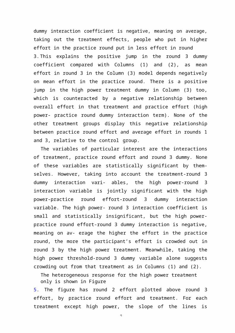
dummy interaction coefficient is negative, meaning on average, taking out the treatment effects, people who put in higher effort in the practice round put in less effort in round3. This explains the positive jump in the round 3 dummy coefficient compared with Columns (1) and (2), as mean effort in round 3 in the Column (3) model depends negatively on mean effort in the practice round. There is a positive jump in the high power treatment dummy in Column (3) too, which is counteracted by a negative relationship between overall effort in that treatment and practice effort (high power- practice round dummy interaction term). None of the other treatment groups display this negative relationship between practice round effort and average effort in rounds 1 and 3, relative to the control group.

The variables of particular interest are the interactions of treatment, practice round effort and round 3 dummy. None of these variables are statistically significant by themselves. However, taking into account the treatment-round 3 dummy interaction variables, the high power-round 3 interaction variable is jointly significant with the high power-practice round effort-round 3 dummy interaction variable. The high power- round 3 interaction coefficient is small and statistically insignificant, but the high power-practice round effort-round 3 dummy interaction is negative, meaning on average the higher the effort in the practice round, the more the participant’s effort is crowded out in round 3 by the high power treatment. Meanwhile, taking the high power threshold-round 3 dummy variable alone suggests crowding out from that treatment as in Columns (1) and (2).

The heterogeneous response for the high power treatment only is shown in Figure

5. The figure has round 2 effort plotted above round 3 effort, by practice round effort and treatment. For each treatment except high power, the slope of the lines is similar in rounds 2 and 3. However, for the high power treatment, the relationship between practice effort and round effort is visibly flatter for round 3 compared with round 2.

3.3 ApplicationsIn this part of the results section the analysis above is carried out for the recorded health and environmental variables and we note some of the interesting findings. It should be stated at the outset that this part of the paper constitutes an analysis of correlations between the

3

crowding out experiment and the health and environmental variables, rather than being a mostly causal story as in Section 3.2.

3.3.1 Healthy behaviours

We start with Table 12, which shows the results of round 1 effort regressed on waist and level of exercise, along with the other controls. We include just waist rather than waist and BMI as waist has a stronger statistical relationship with effort in the practice

Figure 5: Effort (words per minute) in rounds 2 and 3 in terms of effort in practice round, by treatment.

2

2

round and round 1, and BMI and waist are highly correlated (r = 0.78).Column (1) of Table 12 shows waist is a strong predictor of round 1

effort. Column 2 shows people stating they undertook a medium level of exercise (moderate or intensive exercise for at least 30 minutes, 1 to 3 times per week) put in more effort in round 1 than those undertaking a low level of exercise (less than once a week) and those with a high level of exercise (more than 3 times per week). Column (3) shows these statistical relationships hold when both waist and exercise variables are included in the same regression.

Column (4) of Table 12 adds in the important control of age. This additional variable reduces the size of the coefficient on waist size, suggesting part of this effect is due to older participants being more likely to have a larger waist size. However, the coefficient on waist is still statistically significant at the 5% level. The addition of age has little impact on the coefficient on medium exercise. The additional controls are added into Column (5). These controls reduce the size and significance of the coefficient on waist, but do not remove it completely. Finally, practice effort is added into Column (6). As identified in Section 3.2.1, given practice effort is such a strong predictor of round 1 effort, it removes the significance from most coefficients, including waist in this case. However, medium exercise maintains its statistical significance, though the coefficient decreases in size.

Table 13 shows a difference in difference regression for rounds 1 and 2, with interaction terms for level of exercise. In terms of statistical significance for treatment effect, the high power threshold-level of exercise-round 2 interaction variables are negative and significant. This finding means the high power threshold incentive discouraged effort in those who reported that they undertake low or medium levels of exercise, relative to those who exercise frequently. The high power threshold-round 2 and high power threshold-low level of exercise-round 2 coefficients are also jointly significant at the 5% level. No other such pairs of coefficients for round 2 are jointly significant. For round 3, the high power-round 3 and high power-low level of exercise-round 3 coefficients are jointly significant at the 5% level, while the high power-round 3 and high power-medium level of exercise-round 3 coefficients are jointly significant at the 1% level. Thus, while the high power treatment crowds out effort overall in round 3, this crowding out effect is less pronounced for those who undertake low to medium levels of exercise, compared with those who undertake

2

lots of exercise.

3.3.2 Pro-environmental attitudes and behaviours

Table 14 has essentially the same set up as Table 12, except that it uses an environmental attitudes variable – NEP orientation – and an environmental behaviours variable - water sensitive behaviours. Thus, Column (1) shows round 1 effort regressed on NEP orientation only, and there is no statistically significant relationship found. Column

2

Table 12: Round 1 effort regressed on health and demographic variables.

Dependent variable:

Round 1 words/minute(1) (2) (3) (4) (5) (6)


3.478∗∗∗

5.387∗∗∗

5.223∗∗∗

5.245∗∗∗

2.840∗∗∗(0.340) (0.093) (0.349) (0.319) (0.729) (0.503)

Waist −0.022∗∗∗

(0.004)−0.022∗∗∗

(0.004)−0.009∗∗

−0.008∗

(0.004)−0.004(0.003)

Low exercise 0.052 0.003 0.052 0.030 −0.036(0.169) (0.159) (0.145) (0.145) (0.096)

Medium exercise 0.278∗∗

0.243∗∗ 0.263∗∗ 0.260∗∗ 0.146∗∗

(0.130) (0.122) (0.111) (0.110) (0.073)Age −0.025∗∗∗

(0.004)−0.026∗∗∗

(0.005)−0.014∗∗∗

(0.004)Practice effort 0.53

5∗∗∗(0.032)Female 0.057 −0.025

(0.111) (0.073)Education −0.114

(0.191)−0.173(0.126)

Personal income 0.127 −0.208(0.207) (0.138)

Part time −0.203(0.317)

−0.086(0.210)

Unemployed 0.122 −0.163(0.189) (0.126)

Retired −0.230(0.313)

−0.211(0.206)

Postgraduate 0.793 0.146(0.552) (0.367)


−0.205(0.147)

Unable to work −0.183(0.132)

−0.128(0.087)

Other employment

0.142 0.048(0.123) (0.082)

Present bias −0.005 0.020(0.037) (0.024)

Future bias 0.005∗∗ 0.002(0.002) (0.002)


(0.021)

−0.014(0.014)

Observations 229 229 229 229 229 229Adjusted R2 0.121 0.013 0.131 0.280 0.322 0.705F Statistic 32.39

4∗∗∗2.465∗ 12.48

0∗∗∗23.181∗∗∗

7.356∗∗∗

31.209∗∗∗

Note: ∗p<0.1; ∗∗p<0.05; ∗∗∗p<0.01

Notes: Standard errors are in parentheses. Level of exercise dummies are

2

relative to high exercise. Employment status dummies are relative to full time. ∗p<0.1; ∗∗p<0.05; ∗∗∗p<0.01.

3

Table 13: Difference in difference model for rounds 1 to 3, with exercise level interaction terms included.

Dependent variable:

Rounds 1 to 3, words/minuteConstant 3.322∗∗∗ (0.225)Round 2 dummy 0.256∗∗ (0.110)Round 3 dummy 0.533∗∗∗ (0.122)Low power 0.189 (0.324)High power 0.392 (0.274)High power thresh 0.054 (0.290)Charity 0.242 (0.292)Low power*R2 0.189 (0.144)High power*R2 0.059 (0.159)High power thresh*R2 0.224∗ (0.125)Charity*R2 −0.079 (0.131)Low power*R3 −0.022 (0.165)High power*R3 −0.533∗∗∗ (0.196)High power thresh*R3 −0.157 (0.140)Charity*R3 −0.157 (0.162)Low exercise 0.278 (0.504)Medium exercise 0.257 (0.288)Low exercise*R2 0.030 (0.166)Medium exercise*R2 0.008 (0.125)Low exercise*R3 −0.248 (0.206)Medium exercise*R3 −0.186 (0.155)Low p*Low exercise −0.222 (0.694)Low p*Medium exercise −0.322 (0.424)High p*Low exercise −0.281 (0.607)High p*Medium exercise 0.019 (0.353)High p thresh*Low exercise 0.057 (0.557)High p thresh*Medium exercise 0.179 (0.448)Charity*Low exercise −0.754 (0.623)Charity*Medium exercise 0.179 (0.410)Low p*Low exercise*R2 −0.075 (0.225)Low p*Medium exercise*R2 −0.079 (0.174)High p*Low exercise*R2 0.144 (0.277)High p*Medium exercise*R2 0.002 (0.184)High p thresh*Low exercise*R2 −0.688∗∗ (0.274) High p thresh*Medium exercise*R2

−0.288∗∗ (0.143)Charity*Low exercise*R2 0.216 (0.326)Charity*Medium exercise*R2 −0.017 (0.163)Low p*Low exercise*R3 −0.297 (0.367)Low p*Medium exercise*R3 −0.052 (0.206)High p*Low exercise*R3 0.448 (0.463)High p*Medium exercise*R3 0.167 (0.233)High p thresh*Low exercise*R3 −0.039 (0.280)High p thresh*Medium exercise*R3 −0.037 (0.205)Charity*Low exercise*R3 0.449 (0.359)Charity*Medium exercise*R3 0.132 (0.218)

Notes: Standard errors clustered at the individual level are in parentheses. Level of exercise dummies are relative to high exercise. ∗p<0.1; ∗∗p<0.05;

3

∗∗∗p<0.01.

3

(2) shows no statistical relationship between water sensitive behaviours and round 1 effort.

Column (4) shows both NEP and water sensitive behaviours, controlling for age. Once age is controlled for, NEP orientation becomes a statistically significant and positive predictor of round 1 effort. This result holds when the other controls are added in Column (5). Column (6) adds practice round effort and while this variable significantly reduces the size of the coefficient on NEP orientation, the coefficient maintains its statistical significance.

The model estimated in Table 13 is shown using NEP orientation instead of level of exercise in Table 15. There are positive and significant coefficients on the high power-NEP-round 2 and charity-NEP-round 2 interaction terms. These coefficients provide evidence that people with a higher level of pro-ecological orientation respond better to high power incentives, as well as a pro-environmental incentive. In terms of joint significance, the high power-round 2 and high power-NEP-round 2 coefficients are jointly significant at the 10% level, while the high power-round 3 and high power-NEP- round 3 coefficients are jointly significant at the 1% level. Given the positive coefficient on high power-NEP-round 3, the higher NEP participants are less crowded out by the high power incentive - though they are still crowded out to some extent.

4 DiscussionThe results in the practice round and round 1 suggest that some of the demographic variables hold predictive power for intrinsic motivation. As noted in the results section, that age is consistently a strongly statistically significant predictor is likely reflective of the older participants being systematically slower on a computer, rather than due to differences in intrinsic motivation. A different type of task is needed to determine whether intrinsic motivation can vary with age or not. Once age is controlled for, there is no reason to believe skills of the task will vary systematically with any other variables given the low cognitive burden of the task and that it just relies on basic computer skills. The positive correlation between personal income and intrinsic motivation could be related to greater intrinsic motivation helping people earn a higher income. We also tested including household income in the models in Table 8, but it holds no ex- planatory power so

3

we excluded it, which is consistent with intrinsic motivation being important for personal earnings as opposed to household earnings. Why the positive and significant correlation does no hold for education level is not clear, as it would be expected to hold, though the coefficients are positive on education. Another puzzle is why postgraduate students, the unemployed and those unable to work put in significantly more effort in the practice round, compared with full time workers, but not in round 1.

3

Table 14: Round 1 effort regressed on environmental and demographic variables.

Dependent variable:

Round 1 words/minute(1) (2) (3) (4) (5) (6)


4.094∗∗∗

3.740∗∗∗

3.971∗∗∗

3.769∗∗∗

2.334∗∗∗(0.422) (0.370) (0.505) (0.434) (0.745) (0.504)

NEP 0.079 0.118 0.232∗∗ 0.304∗∗∗

0.115∗

(0.112) (0.115) (0.099) (0.100) (0.068)Water sensitive beh.

−0.119

−0.140

−0.020(0.080)

−0.074(0.080)

−0.058(0.054)

Age −0.031∗∗∗

(0.003)−0.033∗∗∗

(0.005)−0.016∗∗∗

(0.003)Practice effort 0.53

5∗∗∗(0.033)Female 0.159 0.024

(0.105) (0.070)Education 0.012 0.028

(0.037) (0.024)Personal income 0.006∗∗ 0.002

(0.002) (0.002)Part time −0.160

(0.192)−0.196(0.128)

Unemployed 0.074 −0.249∗

(0.208) (0.140)Retired −0.067

(0.316)−0.061(0.211)

Postgraduate 0.141 −0.159(0.190) (0.128)


−0.173(0.211)

Unable to work 0.858 0.208(0.551) (0.370)

Other employment −0.078(0.226)

−0.196(0.151)

Present bias −0.206(0.133)

−0.132(0.089)

Future bias 0.075 0.025(0.123) (0.082)


−0.013(0.014)

Observations 226 226 226 226 226 226Adjusted R2 −0.002 0.003 0.004 0.267 0.326 0.701F Statistic 0.498 1.780 1.421 28.29

3∗∗∗7.806∗∗∗

31.979∗∗∗

Note: ∗p<0.1; ∗∗p<0.05; ∗∗∗p<0.01

Notes: Standard errors are in parentheses. Employment status dummies

3

are relative to full time.∗p<0.1; ∗∗p<0.05; ∗∗∗p<0.01.

3

Table 15: Difference in difference model for rounds 1 to 3, with NEP interaction terms included.

Dependent variable:Rounds 1 to 3, words/minute

Constant 3.429∗∗∗ (1.091)Round 2 dummy 0.968∗∗ (0.476)Round 3 dummy 0.511 (0.642)Low power 0.413 (1.318)High power 0.700 (1.445)High power thresh −1.725 (1.428)Charity 0.569 (1.422)Low power*R2 −0.553 (0.611)High power*R2 −1.211∗ (0.629)High power thresh*R2 −0.621 (0.649)Charity*R2 −1.284∗ (0.685)Low power*R3 −0.212 (0.759)High power*R3 −1.047 (0.957)High power thresh*R3 0.143 (0.726)Charity*R3 −0.792 (0.863)NEP 0.013 (0.286)NEP*R2 −0.187 (0.128)NEP*R3 −0.026 (0.167)Low p*NEP −0.111 (0.352)High p*NEP −0.081 (0.376)High p thresh*NEP 0.489 (0.380)Charity*NEP −0.108 (0.387)Low p*NEP*R2 0.184 (0.163)High p*NEP*R2 0.343∗∗ (0.166)High p thresh*NEP*R2 0.166 (0.168)Charity*NEP*R2 0.332∗ (0.191)Low p*NEP*R3 0.033 (0.198)High p*NEP*R3 0.169 (0.240)High p thresh*NEP*R3 −0.082 (0.190)Charity*NEP*R3 0.208 (0.235)

Notes: Standard errors clustered at the individual level are in parentheses. Level of exercise dummies are relative to high exercise. ∗p<0.1; ∗∗p<0.05; ∗∗∗p<0.01.

3

It is interesting that present-biased and more impatient individuals seemed to have lower levels of intrinsic motivation, as an important aspect of having good health behaviours is self control (Promberger and Marteau, 2013). Perhaps patience is a part of intrinsic motivation too. Overall, while there is some predictive power with the demographic variables, there remains plenty of unexplained heterogeneity in observed intrinsic motivation, emphasising the importance of measuring intrinsic motivation as a separate variable for applications in areas such as health and the environment.

In terms of the efficacy of incentives for improving effort, it is interesting that only the low power incentive motivates the participants relative to no incentive (control). All payment treatments, however, lead to greater effort than the charity treatment. The fact that people with a higher NEP score do put in more effort in the charity treatment is an important illustration of the potential heterogeneity of responses to incentives. Given only the low power incentive is an effective motivator, in our context the “pay enough or don’t pay at all” principle does not seem to hold (Gneezy and Rustichini, 2000b). The low power and high power incentives were set at very different levels by design to test extreme values. Future research testing the shape of the supply curve would be useful. At least no decrease in effort is observed in round 2; this highlights the strength of the 4 round design of this experiment, by the fact that we can identify crowding out in rounds 3 and 4. The results in rounds 3 and 4 suggest some interesting dynamics at play in terms of crowding out of intrinsic motivation.

The low power incentive does not significantly crowd out intrinsic motivation, whereas high power and high power threshold incentives do. Thus, in order for the high power incentives to increase effort in round 2, they must increase effort over and above the level of the crowding out that they cause. This they do not achieve. The low power incentive does not have to combat crowding out, given it does not significantly crowd out effort in round 3. Thus, using motivation crowding theory (Frey and Jegen, 2001), the low power incentive is able to increase effort in round 2. The charity treatment has no effect relative to control overall so is effectively pointless in motivating effort in this instance. The fact that the high power incentive crowds out worst amongst the most intrinsically motivated individuals in the first place provides a warning that blanket incentives may end up discouraging the most motivated. Luckily the crowding out effect does

3

fade slightly after the break into round 4, but is still almost as strong for the high power incentive. These results all point to the need for policymakers to be very careful when applying incentives to an area that is previously without incentives. Given the heterogeneous response to the high power treatment, these results suggest the targeting of incentives to particular individuals is an important area for future research. An interesting aspect of targeting of incentives to explore is what effect common knowledge that different people are receiving different incentives would have on crowding out.

3

The health-related behaviours context correlates our results with behaviours that require intrinsic motivation, with largely private benefits. The particular advantage of using the waist measurements is that they are observed and not self-reported by the participants. Thus, it is a useful result for external validity that waist measurements are a predictor of practice round and round 1 effort. That a medium level of exercise also predicts intrinsic motivation whereas high and low exercise does not is a puzzle. In terms of crowding out, the fact that low and medium level exercisers’ effort is crowded out less by the high powered incentives is similar to the result that people with low intrinsic motivation are crowded out less by the high power incentive too. However, the high power incentive still crowds out effort overall in the third round.

The environmental context provides a pro-social application to these results. The NEP variable is shown to be a good predictor of practice round and round 1 effort after controlling for age. The NEP has a large literature validating it as a measure of environmental attitudes and as a good predictor of pro-environmental behaviours (Hawcroft and Milfont, 2010). The number of reported water saving behaviours is a blunt measure of a specific type of pro-environmental behaviours, and thus it did not prove to be a significant predictor of intrinsic motivation. As should be expected, the environmental charity incentive is found to be effective for increasing the round 2 effort of the participants with a high NEP score. Why this holds true for the high power treatment as well is less clear. Contrary to the results that crowding out in the high power treatment is positively related to practice round effort and level of exercise, a high NEP is actually shown to be correlated with lower levels of high power treatment crowding out. This finding is consistent with Grant (2008) in that it suggests that while private intrinsic motivation and pro-social may be correlated, the two types of motivation are not equivalent and may respond differently to incentives. Thus, care must be taken when applying principles from health policy to areas like environmental policy and visa-versa.

4

ReferencesAustralian Bureau of Statistics (2011). Victoria (Main Statistical Area

Structure), Census Data.

B´enabou, R. and J. Tirole (2006). Incentives and Prosocial Behavior. The American Economic Review 96 (5), 1652–1678.

B´enabou, R. and J. Tirole (2011). Identity, Morals, and Taboos: Beliefs as assets. The Quarterly Journal of Economics 126 (2), 805–855.

Cameron, J., K. M. Banko, and W. D. Pierce (2001). Pervasive Negative Effects of Rewards on Intrinsic Motivation: The myth continues. The Behavior Analyst 24 (1), 1.

Deci, E. L. (1971). Effects of Externally Mediated Rewards on Intrinsic Motivation.

Journal of Personality and Social Psychology 18 (1), 105–115.

Deci, E. L., R. Koestner, and R. M. Ryan (1999). A Meta-Analytic Review of Experi- ments Examining the Effects of Extrinsic Rewards on Intrinsic Motivation. Psycho- logical Bulletin 125 (6), 627–668.

Deci, E. L., R. M. Ryan, and R. Koestner (2001). The Pervasive Negative Effects of Re- wards on Intrinsic Motivation: Response to Cameron (2001). Review of Educational Research 71 (1), 43–51.

Dunlap, R. E., K. D. Van Liere, A. G. Mertig, and R. E. Jones (2000). Measuring Endorsement of the New Ecological Paradigm: A revised NEP scale. Journal of Social Issues 56 (3), 425–442.

Erkal, N., L. Gangadharan, and N. Nikiforakis (2011). Relative Earnings and Giving in a Real-Effort Experiment. The American Economic Review 101 (7), 3330–3348.

Fischbacher, U. (2007). z-Tree: Zurich toolbox for ready-made economic experiments.

Experimental Economics 10 (2), 171–178.

Frey, B. S. (1997). On the Relationship Between Intrinsic and Extrinsic Work Motiva- tion. International Journal of Industrial Organization 15 (4), 427–439.

Frey, B. S. and R. Jegen (2001). Motivation Crowding Theory. Journal of Economic Surveys 15 (5), 589–611.

Gillingham, K., D. Rapson, and G. Wagner (2016). The Rebound Effect and Energy Efficiency Policy. Review of Environmental Economics and Policy 10 (1), 68–88.

Gneezy, U., S. Meier, and P. Rey-Biel (2011). When and Why Incentives (Don’t) Work to Modify Behavior. Journal of Economic Perspectives 25 (4), 191–210.

4

Gneezy, U. and A. Rustichini (2000a). A Fine Is a Price. The Journal of Legal Stud- ies 29 (1), 1.

Gneezy, U. and A. Rustichini (2000b). Pay Enough or don’t Pay at all. Quarterly journal of economics, 791–810.

4

Grant, A. M. (2008). Does intrinsic Motivation Fuel the Prosocial Fire? Motivational synergy in predicting persistence, performance, and productivity. Journal of Applied Psychology 93 (1), 48–58.

Hawcroft, L. J. and T. L. Milfont (2010). The Use (and Abuse) of the New Envi- ronmental Paradigm Scale over the Last 30 Years: A meta-analysis. Journal of Environmental Psychology 30 (2), 143–158.

Ma, Q., J. Jin, L. Meng, and Q. Shen (2014). The Dark Side of Monetary Incentive: How does extrinsic reward crowd out intrinsic motivation. NeuroReport 25 (3), 194– 198.

Promberger, M. and T. M. Marteau (2013). When do Financial Incentives Reduce Intrinsic Motivation? Comparing behaviors studied in psychological and economic literatures. Health Psychology 32 (9), 950–957.

Sorrell, S., J. Dimitropoulos, and M. Sommerville (2009). Empirical Estimates of the Direct Rebound eEfect: A review. Energy Policy 37 (4), 1356–1371.

Preface - The University of Western Web viewexperiment on intrinsic motivation and extrinsic...

Documents

Transcript of Preface - The University of Western Web viewexperiment on intrinsic motivation and extrinsic...