J Sched (2007) 10: 271–292DOI 10.1007/s10951-007-0028-6

Preemption in single machine earliness/tardiness scheduling

Kerem Bülbül · Philip Kaminsky · Candace Yano

Published online: 10 August 2007© Springer Science+Business Media, LLC 2007

Abstract We consider a single machine earliness/tardinessscheduling problem with general weights, ready times anddue dates. Our solution approach is based on a time-indexedpreemptive relaxation of the problem. For the objectivefunction of this relaxation, we characterize cost coefficientsthat are the best among those with a piecewise linear struc-ture with two segments. From the solution to the relaxationwith these best objective function coefficients, we generatefeasible solutions for the original non-preemptive problem.We report extensive computational results demonstrating thespeed and effectiveness of this approach.

Keywords Single-machine scheduling · Earliness ·Tardiness · Preemption · Transportation problem

1 Introduction

In the single machine earliness/tardiness (E/T) schedulingproblem, a set of jobs, each with an associated due date, hasto be scheduled on a single machine. Each job has a penaltyper unit time associated with completing before its due date,

K. Bülbül (�)Manufacturing Systems and Industrial Engineering, SabancıUniversity, Istanbul, Turkeye-mail: bulbul@sabanciuniv.edu

P. Kaminsky · C. YanoIndustrial Engineering and Operations Research, University ofCalifornia, Berkeley, CA, USA

C. YanoHaas School of Business, University of California, Berkeley, CA,USA

and a penalty per unit time associated with completing af-ter its due date. E/T problems have been a popular topic ofresearch since the early 1980’s because they reflect the just-in-time (JIT) philosophy, in which early shipments are dis-couraged and result in inventory holding costs in addition tothe tardiness penalties associated with the loss of customergoodwill. Although the single machine E/T problem is use-ful in its own right, our interest in it is further motivated byits appearance as a subproblem in solution approaches formore complex scheduling problems (see Ovacik and Uzsoy1997 and Bülbül et al. 2004). In these more general contexts,it is necessary to solve many such problems very rapidly. Assolution speed is very important, we focus on the develop-ment of fast, effective heuristics for this problem.

Consider a non-preemptive single machine schedulingproblem with n jobs. Associated with each job j , j =1, . . . , n, are several parameters: pj , the processing time forjob j ; rj , the ready time for job j ; dj , the due date for jobj ; εj , the earliness cost per unit time if job j completesprocessing before dj ; and πj , the tardiness cost per unit timeif job j completes processing after dj . We assume that theprocessing times, ready times and due dates are integers. Letsj be the time at which job j starts processing, Cj = sj +pj

be the completion time of job j , and Ej = max(0, dj − Cj )

and Tj = max(0,Cj − dj ) be the earliness and tardiness ofjob j , respectively. The objective is to minimize the sum ofcosts for all jobs. Then our problem is stated as:

(P1) minn∑

j=1

(εj ∗ Ej + πj ∗ Tj ), (1.1)

sj ≥ rj , ∀j, (1.2)

si + pi ≤ sj or sj + pj ≤ si ,

∀i, j, i �= j, (1.3)

272 J Sched (2007) 10: 271–292

sj + pj + Ej − Tj = dj , ∀j, (1.4)

Ej ,Tj ≥ 0, ∀j. (1.5)

The objective is to minimize the total weighted earliness andtardiness. The constraints ensure that jobs start at or aftertheir respective ready times and that jobs do not overlap.

In classifying scheduling problems, we follow the threefield notation of Graham et al. (1979). Problem P1 is repre-sented as 1/rj /

∑(εjEj + πjTj ), where, in the first field,

1 indicates a single machine problem, and the entry rj in thesecond field denotes that the ready times may be unequal. P1is strongly NP-hard because the problem 1/rj /

∑πjTj ,

which is obtained from P1 by setting all earliness costs equalto zero, is known to be strongly NP-hard (Lenstra et al.1977).

We observe that P1 would be a linear program (LP) ifwe knew the sequence of jobs. This is a property of E/Tscheduling problems that is often used to develop a two-phase heuristic: in the first phase, a good job processing se-quence is determined and then, in the second phase, idle timeis inserted either by solving a linear program or by using aspecialized algorithm that exploits the structure of the opti-mal solution with fixed job processing sequences. The sec-ond phase is usually referred to as the optimal timing prob-lem. Researchers have observed that the total cost in E/Tscheduling problems is dominated by the sequencing deci-sions in the first phase; the timing decisions have a smallerimpact. We develop a two-phase heuristic in this paper andfocus on the construction of a good job processing sequencebased on these observations.

Any feasible schedule for P1 is a sequence of blocks sep-arated by idle time, and the cost of a block is a piecewiselinear convex function of the start time of the block. (SeeYano and Kim 1991.) Optimal timing algorithms of low or-der polynomial complexity have been developed for severalspecial cases of P1 using this property (Garey et al. 1988;Davis and Kanet 1993; Szwarc and Mukhopadhyay 1995;Lee and Choi 1995). Also, see Kanet and Sridharan (2000)for an overview of different timing algorithms. For our prob-lem, once jobs are sequenced and assuming jobs are renum-bered in sequence order, the optimal schedule is found bysolving the linear program TT–P1 below.

(TT–P1) minn∑

j=1

(πj ∗ Tj + εj ∗ Ej),

(1.2), (1.4–1.5),

sj + pj ≤ sj+1, ∀j �= n.

Although there exists an O(n2) algorithm for solving theoptimal timing problem for P1 (Nandkeolyar et al. 1993),we use the LP above to determine the final schedule in ourheuristics. LPs for the timing problem are small and take

very little CPU time even if several of them are solved for asingle problem instance.

Many different types of algorithms have been proposedin the literature for various single machine E/T schedul-ing problems. A survey of the early research on earli-ness/tardiness problems appears in Baker and Scudder(1990). More recent research can be found in Kanet andSridharan (2000) and in references therein. In our discussionhere, we restrict our attention to papers that allow idle timein the schedule. Since the problem P1 is strongly NP-hard,most approaches for P1 are either branch and bound (B&B)algorithms or dispatch heuristics based on dominance prop-erties for the job processing sequence. The B&B algorithmsalso make use of these dominance conditions to reduce thesize of the search tree, but none of them is effective for prob-lems with more than 20 to 30 jobs, due to the lack of stronglower bounds for E/T scheduling problems. Szwarc (1993)develops precedence and decomposition rules for the prob-lem 1//ε

∑Ej +π

∑Tj . He proposes a branching scheme

that can handle small problems (n = 10) without a lowerbound. Yano and Kim (1991) devise a B&B algorithm forthe special case of the weighted earliness/tardiness prob-lem, where earliness and tardiness costs are proportionalto the processing times. This property allows them to de-velop dominance properties that are effective, and they cansolve problems with up to 20 jobs optimally. The authorsreport that their lower bounds are loose and further researchis needed for improved lower bounds for their problem. Kimand Yano (1994) and Fry et al. (1996) develop B&B algo-rithms for the mean earliness and tardiness problem. Bothpapers use various adjacency conditions and propose lowerbounds based on elimination of time conflicts. In these pa-pers the authors solve problems with up to 20 jobs optimallywith moderate computation times. Fry and Keong Leong(1987) formulate a mixed integer program for the prob-lem 1//w

∑Cj + ε

∑Ej , which can be expressed as an

equivalent E/T problem, and try to solve it using commer-cial software. For the same problem, Hoogeveen and vande Velde (1996) develop several dominance conditions andlower bounds, and attempt to solve instances with up to 20jobs. They conclude their paper by: “We have consideredan NP-hard machine scheduling problem in which the in-sertion of idle time may be advantageous, and we have pre-sented a branch-and-bound algorithm for its solution. Theallowance of machine idle time complicates the design ofthe algorithm substantially. Also, the performance of the al-gorithm is quite bleak: this is because it is very difficult tocompute strong lower bounds,” which summarizes the dif-ficulties of all B&B approaches for E/T scheduling prob-lems. In fact, one of our major contributions in this paperis the development of a strong lower bound for the problem1/rj /

∑εjEj + πjTj . Also, note that two lower bounds

that are closely related to ours were proposed by Sourd and

J Sched (2007) 10: 271–292 273

Kedad-Sidhoum (2003) and Sourd (2004) and were success-fully implemented in B&B algorithms to solve the problem1//

∑εjEj +πjTj . These authors obtain optimal solutions

for problem instances with 20 jobs within a few seconds,and 30-job instances can be solved to optimality within atmost a few minutes. We discuss the similarities and differ-ences between our research and the approaches presentedby Sourd and Kedad-Sidhoum (2003) and Sourd (2004) inmore detail at the end of this section.

The difficulty of designing effective optimal proce-dures for E/T problems prompted the development of manyheuristics for these problems. Most of these heuristics fol-low a two-phase approach as mentioned above. Examples ofsuch approaches can be found in Fry et al. (1987, 1990), Leeand Choi (1995), Wan and Yen (2002), and Nandkeolyar etal. (1993). The heuristics of Fry et al. (1987) provide solu-tions for the problem 1//

∑εjEj + πjTj , whose objective

values are on average less than 2% above the optimal objec-tive values for problem instances with up to 15 jobs. Simi-larly, for the problem 1//

∑Ej +Tj , Fry et al. (1990) report

that their heuristics provide solutions that are on averagewithin 2.5% of optimality for instances with up to 16 jobs.Lee and Choi (1995) design a genetic algorithm for the prob-lem 1//

∑εjEj + πjTj in which the sequence information

is coded into the chromosomes, and the fitness of the chro-mosomes is evaluated by an optimal timing algorithm. Theircomputational results indicate that their approach is superiorto the heuristics proposed by Yano and Kim (1991). The tabusearch procedure suggested by Wan and Yen (2002) consid-ers a generalization of the problem 1//

∑εjEj + πjTj to

due windows. For relatively small problem instances with15 or 20 jobs, the tabu search finds the optimal solution inover 20% of the cases, and for larger problems it comparesfavorably to incumbent solutions from a B&B algorithm.Ventura and Radhakrishnan (2003) develop a Lagrangian-relaxation-based heuristic for 1//

∑Ej + Tj . They report

that the gap between their best lower bound and best feasiblesolution is less than 3% for problem instances with up to 100jobs. Nandkeolyar et al. (1993), Sridharan and Zhou (1996)and Mazzini and Armentano (2001) consider the problem1/rj /

∑εjEj + πjTj . The latter two papers differ from the

rest of the literature in that they combine sequencing withinsertion of idle time. Sridharan and Zhou (1996) employ alook-ahead procedure at each decision point in order to de-termine whether to keep the machine idle or schedule a jobimmediately. Their solutions are approximately 6% abovethe optimal solution for one problem set with eight-job in-stances, and very close to optimality in another problem setwith up to 40 jobs. Mazzini and Armentano (2001) first se-quence the jobs in non-decreasing order of their respectivetarget start times, i.e., max(rj , dj −pj ), and then insert jobsinto the current partial schedule one by one, consideringpossible idle time. For problems with up to 80 jobs, their al-gorithms provide solutions that are on average within 4.5%

of optimality. (For n ≥ 20, the optimality gaps are computedwith the help of the lower bound developed in this paper.)Note that these authors present one of the very few heuris-tics that simultaneously considers different ready times andweighted earliness and tardiness penalties, and combines se-quencing with insertion of idle time. Thus, we compare theperformance of our heuristics to that of Mazzini and Armen-tano (2001) in Sect. 5.3.3 in order to demonstrate the effec-tiveness of our algorithms. Most of the heuristics mentionedabove can solve problems quickly. However, generally it isnot possible to quantify the quality of their solutions forlarge problem instances because neither optimal solutionsnor tight lower bounds are available for such instances. Oneexception here is the Lagrangian-relaxation-based heuris-tic of Ventura and Radhakrishnan (2003), which providesa lower bound for the problem 1//

∑Ej + Tj . However,

their subgradient algorithm is very slow, taking on average18 minutes to solve their 100-job instances.

In this paper our main contribution is a new strategy forsolving P1. Unlike existing dispatch rules or pairwise in-terchange heuristics for this problem, our algorithms takeinto account all economic trade-offs at the same time andthus are not myopic. We develop a tight lower bound for P1based on a preemptive solution that is easy to compute, andachieves an excellent balance between solution speed andquality. We have two major goals. First, we use the optimalpreemptive solution in developing a good, non-preemptivesolution for P1. Second, we obtain a tight lower bound forspecific instances that can be computed quickly, and is use-ful for quantifying the quality of heuristic solutions. Obtain-ing tight lower bounds has been regarded as a major chal-lenge.

Our algorithms depend on a preemptive relaxation thatis computed by solving a time-indexed problem, in whichwe allow a job to be preempted at integer points in time.(See Sect. 2.) In the time-indexed formulation, we need toconsider a planning horizon whose length depends not onlyon the sum of the processing times but also the due datesbecause both earliness and tardiness costs are present inthe objective function. Hence, from a theoretical viewpointwe compute a lower bound for P1 in pseudo-polynomialtime. However, the time-indexed formulation can be solvedquickly once it is constructed from the original problemdata, and we demonstrate the effectiveness of our approachin the computational experiments in Sect. 5 by solving prob-lem instances of realistic size (with up to 200 jobs). We alsonote that this same lower bound was successfully used insolving subproblems in a column generation algorithm ap-plied to an m-machine flow shop E/T scheduling problem(Bülbül et al. 2004), which is further evidence of the effi-ciency and effectiveness of our lower bound. In addition, theoptimal solution of the preemptive relaxation has sufficientstructure to serve as a starting point for constructing several

274 J Sched (2007) 10: 271–292

feasible solutions which contribute to improving the qualityof the final heuristic solution for P1. Once the lower boundis obtained, feasible solutions are generated very quickly bysolving TT–P1 several times with different job processingsequences. Theoretically, we could even use a special op-timal timing algorithm of complexity O(n2) as mentionedearlier.

The approaches presented by Sourd and Kedad-Sidhoum(2003) and Sourd (2004), developed independently fromour approaches (also see Bülbül 2002), deserve special at-tention here because the lower bounds proposed in thesepapers are closely related to ours. In both of these pa-pers, B&B algorithms are developed to solve the problem1//

∑εjEj + πjTj , and the focus is on obtaining good

lower bounds. In fact, the two B&B algorithms differ onlyin the computation of the lower bounds, which are based ondifferent preemptive relaxations. Two major factors affectthe quality of the lower bounds obtained from these relax-ations: the preemption scheme, i.e., when and for how longa job can be preempted, and the objective function of therelaxation. (See Sect. 2.) Sourd and Kedad-Sidhoum (2003)consider a time-indexed preemptive relaxation, in which ajob can be preempted at integer points in time, as in ourapproach. However, Sourd (2004) proposes a different ap-proach, in which each job may be preempted at any pointin time. A lower bound for the problem 1//

∑εjEj + πjTj

can be computed in polynomial time, when based on a con-tinuous relaxation rather than a time-indexed one. These au-thors observe that the two B&B algorithms perform simi-larly despite the theoretical differences in the lower bounds.Both Sourd and Kedad-Sidhoum (2003) and Sourd (2004)consider a family of valid objective functions for their re-spective relaxations and heuristically choose one for theircomputational experiments. Here, we follow a different pathand develop an objective function for our preemptive relax-ation based on an intuitively simple observation in Sect. 2. InSect. 3.2 this objective function is shown to be optimal withrespect to certain criteria and, interestingly, it also turns outto be closely related to the objective function developed forthe continuous relaxation by Sourd (2004). In other words,our research provides the link between the “discrete” and“continuous” lower bounds proposed by Sourd and Kedad-Sidhoum (2003) and Sourd (2004), respectively. We elab-orate further on this issue in the next section. Finally, oneof our major emphases is the construction of good feasiblesolutions for the original problem after the optimal solutionof the preemptive problem is obtained. Sourd and Kedad-Sidhoum (2003) and Sourd (2004) pay less attention to thisphase of the solution procedure. In Sect. 5 we demonstratethat our lower bound exhibits some desirable properties thatlead to a more stable behavior in obtaining good feasiblesolutions for P1.

In Sect. 2 we review some general properties of preemp-tive E/T problems that lead us to an appropriate preemption

strategy for P1. Then we develop a penalty scheme for thispreemptive relaxation and we show that a formulation basedon this scheme leads to an excellent lower bound for P1.In Sect. 3 we derive some properties of our lower bound.In Sect. 4 we present an heuristic that uses the informa-tion from the optimal solution of the preemptive relaxationto create a feasible solution for P1. Finally, in Sect. 5 wepresent the results of our computational experiments whichdemonstrate the effectiveness of our lower bound and of ourheuristics. We conclude in Sect. 6.

2 A lower bound for P1

The complexity of a preemptive scheduling problem de-pends strongly on the penalty scheme applied to differentjob segments. If only the last portion of a job may incura non-zero cost in a preemptive E/T scheduling problem1/prmp/

∑(εjEj +πjTj ), then earliness costs can be made

negligibly small by scheduling an arbitrarily small portionof duration δ > 0 to complete at time dj for any early job j

(Mosheiov 1996). Hence, under this cost structure we cantreat 1/prmp/

∑(εjEj + πjTj ) as a preemptive weighted

tardiness problem 1/prmp/∑

πjTj , for which every pre-emptive schedule can be transformed into a non-preemptiveschedule with no larger objective value (McNaughton 1959).Therefore, both problems 1/prmp/

∑πjTj and 1/prmp/∑

(εjEj +πjTj ) are as hard as the non-preemptive weight-ed tardiness problem 1//

∑πjTj , which is known to be

NP-hard (see Lenstra et al. 1977). So, we conclude that apreemptive E/T scheduling problem, in which only the lastportion of a job may incur a non-zero cost, is unlikely toprovide a tight lower bound for P1. However, we highlightan important property of the weighted tardiness problem. Ifall jobs have unit processing times, then a non-preemptiveweighted tardiness problem can be solved in polynomialtime because it is equivalent to a transportation problem.This result leads us to a different preemption scheme in or-der to develop a lower bound for P1.

Our approach for constructing a lower bound buildsupon the ideas of Gelders and Kleindorfer (1974) for thesingle machine weighted tardiness problem and the re-sults of Verma and Dessouky (1998) for the single ma-chine non-preemptive weighted E/T scheduling problemwith unit processing times. To obtain a lower bound, Geldersand Kleindorfer divide each job into unit-duration intervals(jobs) and associate a cost with each unit job. We utilize theiridea of unit-duration jobs and allow a job to be preempted atinteger points in time. Their other results, however, cannotbe used directly because their objective function differs fromours, and non-delay schedules are optimal in weighted tardi-ness problems, but may be suboptimal when earliness costsare considered. We also note that the form of preemption that

J Sched (2007) 10: 271–292 275

we consider is often implemented in practical applications,due to the nature of the manufacturing process or the struc-ture of the work schedule, by simply dividing customer or-ders into smaller processing batches in an appropriate way.Thus, although our study was motivated partly by theoreticalconsiderations, the results may be useful in practice.

We first present some properties of the optimal solutionof P1 that lead us to a transportation problem, whose optimalobjective value is a lower bound on that of P1. We state thefollowing property without proof. The reader is referred toSourd and Kedad-Sidhoum (2003) for a formal proof of asimilar property for the problem 1//

∑εjEj + πjTj .

Property 2.1 If processing times, due dates and ready timesare integers, then there exists an optimal solution for P1 inwhich all job completion times are integers.

Without loss of generality, Property 2.1 indicates that thesolution space can be restricted to integer start times. In-tuitively, an approximation to P1 could be obtained by di-viding each job j into pj unit-duration jobs, associating apenalty with each unit job (rather than only with the lastone completed) and planning for a horizon consisting of anappropriate integral number time periods. Before doing so,we restate P1 as an equivalent binary non-linear program.Then we discuss modifications to this problem that lead toa relaxation, from which we derive a lower bound. In thetime-indexed formulations in this paper, a period k spansfrom time k − 1 to k; hence, a job j with ready time rj canbe processed no earlier than in period rj + 1. Let Xjk = 1if job j is processed in period k, and 0 otherwise; and let(x)+ = max(x,0). So we have:

(P2) min∑

j

∑

k∈H

[εj (dj − k)+ + πj (k − dj )

+]

∗ (Xjk − Xjk+1)+, (2.1)

∑

k∈H

Xjk = pj , ∀j, (2.2)

∑

j

Xjk ≤ 1, ∀k ∈ H, (2.3)

∑

k∈H

(Xjk − Xjk+1)+ = 1, ∀j, (2.4)

Xjtmax+1 = 0, ∀j, (2.5)

Xjk ∈ {0,1}, ∀j, k ∈ H ∪ {tmax + 1}. (2.6)

Let tmin = minj rj +1, tmax = maxj max(rj , dj )+P , whereP = ∑

j pj is the sum of processing times. Also let theplanning horizon be H , and define H = {k | k ∈ Z, k ∈[tmin, tmax]}. Thus, the maximum value of k in H is greaterthan or equal to the latest period in which any portion of anyjob could conceivably be processed in an optimal solution,

accounting for potential idle time. In the non-preemptiveproblem, the expression (Xjk −Xjk+1)

+ takes the value oneonly if k is the completion time of job j and is zero, other-wise. So the term in square brackets in the objective func-tion is the cost incurred if job j finishes in period k. Theconstraints (2.2) and the contiguity constraints (2.4–2.5) to-gether ensure that each job j is processed in pj consecutiveperiods. The machine can process at most one job in anygiven period as specified by constraints (2.3).

Now we present a new formulation obtained by omittingthe contiguity constraints and replacing the objective func-tion with a simpler expression, in which each unit-durationportion of each job has an associated cost coefficient:

(TR) min∑

j

∑

k∈Hk≥rj +1

cjkXjk, (2.7)

∑

k∈Hk≥rj +1

Xjk = pj , ∀j, (2.8)

∑

jk≥rj +1

Xjk ≤ 1, ∀k ∈ H, (2.9)

Xjk ≥ 0, ∀j, k ∈ H, k ≥ rj + 1. (2.10)

This new formulation is equivalent to a transportation prob-lem. Hence, the binary constraints do not need to be statedexplicitly, and the problem can be solved very efficiently.The idea underlying our proposed cost structure is intuitive.If a non-preemptively scheduled job j finishes exactly at dj ,and if we think of each of the pj unit-duration segments injob j as different jobs, then the average completion time ofthese unit-duration segments is

(dj − pj + 1) + · · · + dj

pj

= dj − 1 + · · · + (pj − 1)

pj

= dj − (pj − 1)pj

2pj

= dj −(

pj

2− 1

2

).

We treat dj − (pj

2 − 12 ), this average time, as the common

due date for all unit jobs within job j and assign the follow-ing cost coefficients:

cjk =⎧⎨

⎩

εj

pj

[(dj − pj

2

) − (k − 1

2

)], k ≤ dj ,

πj

pj

[(k − 1

2

) − (dj − pj

2

)], k > dj .

(2.11)

Below we provide our main result in this section: a proof thatthe solution of TR with the coefficients given above providesa lower bound on the optimal objective function value ofP1. Furthermore, in Sect. 3.2 we prove that this set of costcoefficients is a very good candidate to maximize the valueof the lower bound obtained from TR. Now let SP represent a

276 J Sched (2007) 10: 271–292

feasible schedule for problem P with a total cost of TC(SP).An optimal schedule is denoted by an asterisk.

Theorem 2.2 The optimal objective value of TR, TC(S∗TR),

is a lower bound on the optimal objective value TC(S∗P1) of

P1.

Proof We show that for any optimal solution S∗P1 for P1,

there exists a corresponding feasible schedule STR for TRsuch that TC(STR) ≤ TC(S∗

P1). In particular, we considera solution STR for TR constructed by converting S∗

P1 intoa feasible solution of TR. This is accomplished by divid-ing each job in S∗

P1 into contiguous unit-duration segments.We demonstrate that for a schedule STR constructed in thismanner, TC(STR) ≤ TC(S∗

P1). Clearly, an optimal solutionS∗

P1 for P1 exists in which all job completion times belongto H = {k | k ∈ Z, k ∈ [tmin, tmax]}, which is the same timehorizon considered in problem TR. Our strategy is to con-sider each job in S∗

P1 separately. If Cj ≤ dj in S∗P1, then the

cost that job j incurs in STR is given by:

Cj∑

k=Cj −pj +1

cjk = εj

pj

Cj∑

k=Cj −pj +1

[(dj − pj

2

)−

(k − 1

2

)]

= εj (dj − Cj ),

as in S∗P1. If job j is tardy in S∗

P1, then we need to distinguishbetween two cases. If Cj ≥ dj + pj , then the cost that job j

incurs in STR is given by:

Cj∑

k=Cj −pj +1

cjk = πj

pj

Cj∑

k=Cj −pj +1

[(k − 1

2

)−

(dj − pj

2

)]

= πj (Cj − dj ),

as in S∗P1. However, if dj + 1 ≤ Cj ≤ dj + pj − 1 when

pj ≥ 2, then x = Cj − dj unit jobs of job j incur a tardinesscost in STR, while the remaining (pj − x) unit jobs incur anearliness cost. In this case the cost incurred by job j in STR

consists of two parts:

Cj∑

k=Cj −pj +1

cjk =dj +x∑

k=dj +x−pj +1

cjk

=dj∑

k=dj +x−pj +1

cjk +dj +x∑

k=dj +1

cjk, (2.12)

where 1 ≤ x ≤ pj − 1. We first examine the costs incurredby the unit jobs completed at or before dj :

dj∑

k=dj +x−pj +1

cjk = εj

pj

[−xpj

2+ x2

2

]

= εj

pj

[x

2(x − pj )

]< 0

(because x < pj ). (2.13)

Next, we examine the costs incurred by the unit jobs com-pleted after dj :

dj +x∑

k=dj +1

cjk = πj

pj

[x

2(x + pj )

]= πjx

[x + pj

2pj

]< πjx

(because x < pj ). (2.14)

Therefore, we have∑Cj

k=Cj −pj +1 cjk < πjx = πj (Cj − dj )

when dj + 1 ≤ Cj ≤ dj +pj − 1. Finally, summing over alljobs, we obtain TC(S∗

TR) ≤ TC(STR) ≤ TC(S∗P1), as desired,

because the cost incurred by any job j in STR is no largerthan that in S∗

P1. �

Note that we must account for the possibility that someunit jobs may be early and some others may be tardy for ajob j of duration pj > 1 in a non-preemptive feasible so-lution of TR. This property complicates the task of find-ing an appropriate cost structure, and the proof of Theo-rem 2.2 provides a critical insight: job j incurs the samecost in S∗

P1 and STR, unless it finishes in the time interval[dj + 1, dj + pj − 1]. We use this property in proving someof our results in Sect. 3, where we derive the cost that job j

incurs in STR when dj ≤ Cj ≤ dj + pj . From (2.12–2.14),we have

Cj∑

k=Cj −pj +1

cjk = f (x) =dj +x∑

k=dj +x−pj +1

cjk

= 1

2

(εj

pj

+ πj

pj

)x2 + 1

2(πj − εj )x, (2.15)

where 0 ≤ x = Cj − dj ≤ pj .Sourd and Kedad-Sidhoum (2003) propose a lower

bound similar to ours for the problem 1//∑

εjEj + πjTj

based on a transportation problem with the following costcoefficients:

c′jk =

⎧⎪⎪⎨

⎪⎪⎩

⌊ (dj −k)

pj

⌋εj , k ≤ dj − pj ,

0, dj − pj + 1 ≤ k ≤ dj ,⌈ (k−dj )

pj

⌉πj , k ≥ dj + 1.

(2.16)

Note that these coefficients form a (discrete) step func-tion, and they stay constant for pj consecutive periods. Sothey have a different structure than our cost coefficients

J Sched (2007) 10: 271–292 277

given in (2.11). Also, the cost coefficients in (2.16) satisfy∑Cj

k=Cj −pj +1 c′jk = εjEj + πjTj for all possible comple-

tion times Cj . Recall that this condition is not satisfied byour cost coefficients when job j finishes in the time inter-val [dj + 1, dj + pj − 1]. However, we note that c′

jk < cjk

for some periods k. Therefore, it is not clear a priori whichset of cost coefficients will perform better in practice. InSect. 5, we compare these cost coefficients computationally,and conclude that TR generally yields tighter lower boundswhen our cost coefficients in (2.11) are used.

Sourd (2004) develops a polynomial-time lower boundfor the problem 1//

∑εjEj +πjTj based on the continuous

assignment problem (see Sect. 1). In other words, he allowsa job to be preempted at any point in time, and defines a cost

function fj (t) such that∫ Cj

Cj −pjfj (t) dt ≤ εjEj + πjTj for

all possible completion times Cj . In particular, he proposesusing

fj (t) =⎧⎨

⎩− εj

2 + εj

pj(dj − t), t ≤ dj ,

πj

2 + πj

pj(t − dj ), t > dj ,

(2.17)

when εj > πj , and a slightly different cost function whenεj ≤ πj . We observe that our cost coefficients in (2.11) canbe obtained by setting:

cjk =∫ k

k−1fj (t) dt. (2.18)

Hence, we have∫ Cj

Cj −pjfj (t) dt = ∑Cj

k=Cj −pj +1 cjk . In

other words, our “discrete” lower bound is closer to the“continuous” lower bound of Sourd (2004) than to the dis-crete lower bound presented in Sourd and Kedad-Sidhoum(2003). Sourd (2004) reports that the lower bound basedon the continuous assignment problem and (2.17) gener-ally performs better than the discrete lower bound based on(2.16), which also agrees with our computational experiencein Sect. 5. Furthermore, in Sect. 3.2 we prove that the costcoefficients given in (2.11) are, in some sense, the optimalcost coefficients for TR when the cost coefficients are re-stricted to lie on a piecewise linear function with only twosegments (see Theorem 3.2). So there is both theoretical andpractical justification for using our cost coefficients in orderto obtain a good lower bound for P1.

In TR there are n + (tmax − tmin + 1) constraints and atmost n ∗ (tmax − tmin + 1) variables. It is possible, however,to state an equivalent transportation problem with at mostn+2nP constraints and at most 2nP variables by observingthat there exists an optimal solution to TR such that Xjk

must be zero if k does not belong to the set Hj = {k | k ∈Z, k ∈ [max(rj + 1, dj − P + 1), dj + P ]}. This propertyis similar to Lemma 2.1 in Verma and Dessouky (1998). Inour computational experiments, we observed that although

this property does not usually change the number of nodesin the transportation problem (the sum of the number of jobsand the number of time periods in the planning horizon), itdecreases the number of arcs (number of variables) by 30 to50%, depending on the problem instance.

From a theoretical perspective, obtaining a lower boundfor P1 from TR is accomplished in pseudo-polynomial time,since the planning horizon depends on the sum of theprocessing times (also see Sect. 1). However, in practicethere are several advantages to this approach that allow usto develop effective algorithms for solving P1 based on theoptimal solution of TR. First, the transportation problem canbe solved quickly even for very large instances. Sourd andKedad-Sidhoum (2003) note that all pj unit jobs of a jobj are identical, and they exploit this property to developan adaptation of the Hungarian algorithm for solving theirtransportation problem. They reduce the complexity of theHungarian algorithm from O(|H |3) to O(n2|H |) for thisclass of transportation problems, where |H | is the numberof periods in the planning horizon. (We do not use this spe-cialized algorithm in our computational experiments.) Sec-ond, the optimal solution of the transportation problem al-lows us to construct several feasible solutions for P1 withvery little additional computational effort once problem TRis solved. Clearly, this increases the likelihood of finding anear-optimal feasible solution for P1 (see Sects. 4 and 5).Finally, we observe that the size of the transportation prob-lem is relatively smaller for computationally hard instancesof P1. Intuitively, if the due dates are close to each other andjobs compete with each other to be scheduled in the sametime periods, then such an instance is harder to solve. How-ever, when the due dates are close to each other, then wehave a relatively smaller instance of the transportation prob-lem.

3 Properties of the lower bound

In this section we characterize a portion of the gap betweenthe objective from our lower bound, TC(S∗

TR), and the op-timal objective value. We observe that any gap between thecost of S∗

TR and that of S∗P1 is partly due to preemption in the

transportation solution and partly due to the different coststructures. In this section we explore the second effect indetail.

First, consider a single-job instance of problem P1.Clearly, if there is only a single job j and rj + pj ≤ dj ,then for all possible values of εj > 0 and πj > 0, job j isscheduled in the interval [dj −pj , dj ] in an optimal solutionS∗

P1 with a total cost of zero. Similarly, job j is schedulednon-preemptively in the interval [dj − pj , dj ] in an opti-mal transportation solution S∗

TR with a total cost of zeroif πj ≥ εj . We can show this by using the convexity of f

278 J Sched (2007) 10: 271–292

and f′(0) ≥ 0, where f (x) is the cost incurred by job j

in TR when it is scheduled non-preemptively in the interval[dj +x −pj , dj +x], as described in (2.15). However, whenπj < εj , there is an incentive to complete job j strictly afterits due date in TR. Note that f

′(0) < 0 if πj < εj . In fact,

when pj > 1, we can easily create single-job instances forwhich S∗

TR differs from S∗P1, and we can make TC(S∗

TR) ar-bitrarily smaller than TC(S∗

P1) by increasing the difference(εj − πj ).

From the discussion above we conclude that, as long asεj ≤ πj ∀j , the optimal objective value of TR cannot bestrictly less than zero, and we cannot create pathological in-stances for which TR yields arbitrarily poor lower bounds.We observe that the cost structure εj ≤ πj ∀j implies thatthe cost of loss of customer goodwill per unit time is at leastas expensive as the finished goods inventory holding costper unit time. In general, we would expect this to be rea-sonable for most just-in-time systems, as just-in-time usu-ally implies minimizing inventory costs, subject to meetingcustomer due dates. However, we emphasize again that ourlower bound and our heuristics for P1 do not make any spe-cific assumption about the cost structure. In fact, our com-putational results in Sect. 5.3.3 indicate that our algorithmsare not sensitive to it.

Next, for any given non-preemptive schedule we charac-terize the largest possible difference between its associatedobjective function values in problems TR and P1. Then, inSect. 3.2, we prove that the cost coefficients developed forTR in the previous section are, in some sense, the best pos-sible cost coefficients.

3.1 Cost function difference for identical schedules

In Sect. 2 we proved that TC(S∗TR) is a lower bound on

TC(S∗P1). In this section we give two characterizations of the

portion of the gap attributable to the difference between theobjective functions of P1 and TR. To motivate the discus-sion, suppose that we develop an algorithm that converts S∗

TRinto a non-preemptive schedule SP1, and we are interestedin computing a bound on the worst case difference betweenTC(SP1) and TC(S∗

TR). To accomplish this, one would needto account for both the increase in the objective of TR whileconstructing SP1 from S∗

TR, and the increase in cost from ap-plying the original objective function to SP1. The followinglemma characterizes the latter increase both in terms of theabsolute and relative difference in cost, when the objectivefunctions of TR and P1 are applied to the same (not neces-sarily optimal) non-preemptive schedule. In this lemma, ifjob j completes processing at time Cj in a feasible schedulefor the original non-preemptive problem P1, then Xjk = 1for all k = Cj − pj + 1, . . . ,Cj in the corresponding trans-portation solution STR. Refer to Bülbül (2002) for a proof.

Lemma 3.1 Let SP1 be a feasible schedule for the originalnon-preemptive problem P1 with a cost of TC(SP1), and letSTR be the corresponding transportation solution with a costof TC(STR). Then

TC(SP1) − TC(STR) ≤ 1

8

n∑

j=1

(πj + εj )pj . (3.1)

If, in addition, εj ≤ πj , ∀j , then we also have

0 ≤ TC(STR) ≤ TC(SP1) ≤ pmax ∗ TC(STR). (3.2)

The proof of (3.2) also suggests that our lower bound be-comes tighter, when the tardiness costs increase relative tothe earliness costs. This implies that our lower bound mayalso be useful for solving weighted tardiness problems. Inaddition, according to (3.2), the optimal objective functionvalue of TR is the same as that of P1 if all jobs are of unitlength, i.e., pmax = 1. Note that this is true even if thereexists a job j such that εj > πj (see Verma and Dessouky1998). Finally, we note that the bound provided in (3.2) hasthe desirable property of being independent of the earlinessand tardiness costs.

3.2 Optimal linear cost coefficient function

At the beginning of Sect. 3 we discussed that the differencebetween the cost function of TR (for a single job) and thecost function of P1 can be relatively large in the worst case.A natural question to ask is whether we can find cost coef-ficients that will decrease the difference between the costsincurred by the same non-preemptive schedule in P1 and inTR, and, thereby, improve the bounds given in Lemma 3.1.We restrict ourselves to linear cost coefficient functions, asdefined below. This choice has a natural appeal for three rea-sons. First, the original problem P1 also has a linear penaltystructure. Second, the lower bound obtained from TR basedon the piecewise linear cost structure in (2.11), and the non-preemptive schedules adapted from S∗

TR perform very well,as we demonstrate in the computational experiments. Fi-nally, linearity enables us to use linear programming dualityto prove our result. Specifically, we look for cost coefficientscjk for job j that satisfy the following conditions, where mE

and mT represent the slope of the cost function before andafter the due date dj , respectively

cjk = cjdj+ (dj − k) ∗ mE, ∀k ≤ dj , (3.3)

cjk = cjdj +1 + (k − dj − 1) ∗ mT , ∀k ≥ dj + 1, (3.4)

mE,mT ≥ 0. (3.5)

Next, we need to choose an appropriate objective functionthat reflects how “good” the cost coefficients are. Note thatall we know about the completion time Cj of job j in an

J Sched (2007) 10: 271–292 279

optimal non-preemptive schedule is that it lies within someinterval H (see Sect. 2). This implies that we need cost co-efficients that perform well over a range of possible comple-tion times rather than for a specific completion time. Nowassume that Cj lies in some interval [tjmin, t

jmax] that in-

cludes dj , and let TCj (SP) denote the cost incurred by jobj in problem P. As alternatives for the objective function,we consider minimizing the maximum or the total differ-ence of TCj (SP1) − TCj (STR) across all Cj values in the

interval [tjmin, tjmax]. Note that we concern ourselves with the

cost function of a single job here, and we can, therefore, re-strict our attention to non-preemptive schedules without lossof generality. We observed computationally that the optimalcost coefficients are dependent on the choices of t

j

min and

tjmax for the minimax criterion. However, as we prove in this

section, the optimal cost coefficients for the minisum objec-tive are not contingent on the specific values of these two pa-rameters under some mild conditions. Additionally, by solv-ing several instances, we also observed that the optimal so-lution for the minimax criterion becomes more similar tothe optimal solution of the minisum criterion as t

jmax − t

j

minincreases. Therefore, we use the minisum criterion and char-acterize the structure of its optimal solution in the followingdiscussion.

The problem of finding cost coefficients that satisfy(3.3) through (3.5) and minimize the objective function∑

Cj ∈[tjmin,tjmax](TCj (SP1) − TCj (STR)) when job j is sched-

uled non-preemptively to finish at the same time both in SP1

and STR can be represented as a linear programming prob-lem. Let aE and aT denote cjd and cjd+1, respectively, andDt be TCj (SP1) − TCj (STR) if job j finishes processing at

time t . Also, let tj

min and tjmax be the smallest and largest

possible completion times of job j , respectively. In general,we allow t

j

min ≥ rj + pj and tjmax ≤ dj + P , and later in

the discussion we identify some mild conditions that needto be imposed on t

j

min and tjmax. In the following linear pro-

gramming problem we omit the job index j to simplify thenotation:

(CP) mintmax∑

t=tmin

Dt, (3.6)

(γt ) Dt +t∑

k=t−p+1

(aE + (d − k)mE

) = ε(d − t),

t = tmin, . . . , d, (3.7)

(δt ) Dt +d∑

k=t−p+1

(aE + (d − k)mE

)

+t∑

k=d+1

(aT + (k − d − 1)mT

) = π(t − d),

t = d + 1, . . . , d + p − 1, (3.8)

(μt ) Dt +t∑

k=t−p+1

(aT + (k − d − 1)mT

) = π(t − d),

t = d + p, . . . , tmax, (3.9)

aE,aT unrestr., (3.10)

mE,mT ≥ 0, (3.11)

Dt ≥ 0, t = tmin, . . . , tmax. (3.12)

Constraints (3.7) through (3.9) define the difference in pe-riod t , Dt , between the cost functions of TR and P1 fordifferent completion times of job j . By (3.12), TCj (SP1) −TCj (STR) is guaranteed to be nonnegative for all possiblecompletion times of job j . Thus, TC(S∗

TR) yields a lowerbound on TC(S∗

P1) for all objective function coefficients cjk ,generated from any feasible solution of CP. The Greek let-ters on the left are the dual variables associated with the con-straints.

Now we show that the optimal solution to CP corre-sponds to the cost coefficients (2.11) when tmin ≤ d − p

and tmax ≥ d + 2p. In practice, these conditions are au-tomatically satisfied for the great majority of problem in-stances. From the definition of the planning horizon H ,it follows that all we require is rj + pj ≤ dj − pj anddj + P ≥ dj + 2pj , i.e., dj − rj ≥ 2pj and P ≥ 2pj .

Theorem 3.2 If tmin ≤ d − p and tmax ≥ d + 2p, then theoptimal solution to CP is given by mE = ε

p, mT = π

p, aE =

εp(−p2 + 1

2 ), and aT = πp(p2 + 1

2 ), which correspond to thecost coefficients

ck ={

εp

[(d − p

2

) − (k − 1

2

)], k ≤ d ,

πp

[(k − 1

2

) − (d − p

2

)], k > d ,

given in (2.11). The optimal objective function value is112 (ε + π)(p2 − 1).

Proof Our strategy is to find a feasible dual solution with thesame objective value given above. It follows directly fromTheorem 2.2 that mE = ε

p≥ 0, mT = π

p≥ 0, aE = ε

p(−p2 +

12 ), aT = π

p(p2 + 1

2 ), and the corresponding Dt values arefeasible for CP. The resulting objective function value is∑tmax

t=tminDt = ∑p−1

x=1 (πx − f (x)) = 112 (ε + π)(p2 − 1),

using (2.15) and the identities∑n

k=1 k = n(n+1)2 and

∑nk=1 k2 =

n(n+1)(2n+1)6 . The dual of CP is:

(DCP) maxd∑

t=tmin

ε(d − t)γt +d+p−1∑

t=d+1

π(t − d)δt

+tmax∑

t=d+p

π(t − d)μt , (3.13)

280 J Sched (2007) 10: 271–292

(Dt ) γt ≤ 1, t = tmin, . . . , d, (3.14)

(Dt ) δt ≤ 1, t = d + 1, . . . , d + p − 1, (3.15)

(Dt ) μt ≤ 1, t = d + p, . . . , tmax, (3.16)

(aE)

d∑

t=tmin

pγt +p−1∑

t=1

(p − t)δd+t = 0, (3.17)

(aT )

p−1∑

t=1

tδd+t +tmax∑

t=d+p

pμt = 0, (3.18)

(mE)

d∑

t=tmin

t∑

k=t−p+1

(d − k)γt

+d+p−1∑

t=d+1

d∑

k=t−p+1

(d − k)δt ≤ 0, (3.19)

(mT )

d+p−1∑

t=d+1

t∑

k=d+1

(k − d − 1)δt

+tmax∑

t=d+p

t∑

k=t−p+1

(k − d − 1)μt ≤ 0,

(3.20)

γt unrestr., t = tmin, . . . , d, (3.21)

δt unrestr., t = d + 1, . . . , d + p − 1,

(3.22)

μt unrestr., t = d + p, . . . , tmax. (3.23)

The corresponding primal variable for each constraint is in-dicated in parentheses on the left. A proof of the followinglemma is presented by Bülbül (2002).

Lemma 3.3 If tmin ≤ d − p and tmax ≥ d + 2p, then thefollowing solution is feasible for DCP.

γtmin = −γd − p − 1

2− K + 1,

where K = d − tmin, (3.24)

γt = 1, tmin + 1 ≤ t ≤ d − 1, (3.25)

γd = −(p + 1)(p − 1)

12K− K + p

2+ 1, (3.26)

δt = 1, d + 1 ≤ t ≤ d + p − 1, (3.27)

μd+p =N2

2 + N(−p2 − 1) + (p − 1)(

p+1312 ) + 1

−N + p,

where N = tmax − d, (3.28)

μt = 1, d + p + 1 ≤ t ≤ tmax − 1, (3.29)

μtmax = −μd+p − p − 1

2− N + p + 1. (3.30)

We now compute the objective function value for this dualfeasible solution to complete the proof. First, we computethe following three expressions:

d∑

t=tmin

(d − t)γt

= (d − tmin)γtmin +d−tmin−1∑

t=1

t

= K

((p + 1)(p − 1)

12K+ K + p

2− 1 − p − 1

2− K + 1

)

+ K(K − 1)

2

= (p + 1)(p − 1)

12,

d+p−1∑

t=d+1

(t − d)δt =p−1∑

t=1

t = p(p − 1)

2,

tmax∑

t=d+p

(t − d)μt

= pμd+p + (p + 1) + (p + 2) + · · · + (N − 1)

+Nμtmax

= pμd+p + (N − p − 1)p

+N−p−1∑

t=1

t + N

(−μd+p − p − 1

2− (N − 1 − p)

)

= (p + 1)(p − 1)

12− p(p − 1)

2.

Therefore, the objective function value for the dual feasiblesolution given in (3.24–3.30) is:

d∑

t=tmin

ε(d − t)γt +d+p−1∑

t=d+1

π(t − d)δt +tmax∑

t=d+p

π(t − d)μt

= ε(p + 1)(p − 1)

12

+π

(p(p − 1)

2+ (p + 1)(p − 1)

12− p(p − 1)

2

)

= 1

12(ε + π)(p + 1)(p − 1) = 1

12(ε + π)(p2 − 1),

which is equal to the objective function value of the primalfeasible solution mE = ε

p, mT = π

p, aE = ε

p(−p2 + 1

2 ), aT =πp(p2 + 1

2 ), and the corresponding Dt values. �

J Sched (2007) 10: 271–292 281

Note that the conditions tmin ≤ d − p and tmax ≥ d + 2p

are sufficient, but not necessary, for the coefficients in The-orem 3.2 to be optimal. For instance, assume d = 10, p = 4,ε = 1, π = 1. Choose tmin = 8 > d −p and tmax = 14 < d +2p. Then the optimal solution to CP is mE = 0.25, mT = 0,aE = −0.375, and aT = 1. These values satisfy mE = ε

p

and aE = εp(−p2 + 1

2 ), but not mT = πp

and aT = πp(p2 + 1

2 ),i.e., the cost coefficients characterized in Theorem 3.2 arenot optimal. The planning horizon extends for such a shortduration after the due date that the optimal cost coefficientsare constant in the interval [11,14]. However, if tmax is in-creased to d + 2p = 18, then the cost coefficients in Theo-rem 3.2 are optimal, even if d − tmin < p.

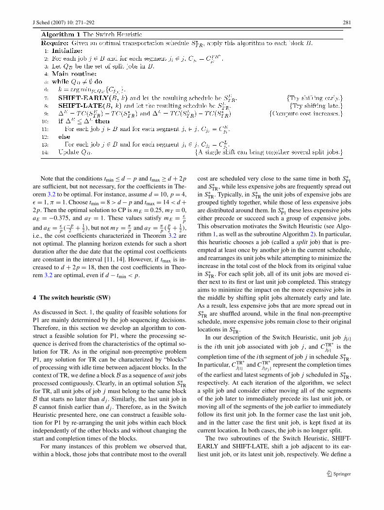
4 The switch heuristic (SW)

As discussed in Sect. 1, the quality of feasible solutions forP1 are mainly determined by the job sequencing decisions.Therefore, in this section we develop an algorithm to con-struct a feasible solution for P1, where the processing se-quence is derived from the characteristics of the optimal so-lution for TR. As in the original non-preemptive problemP1, any solution for TR can be characterized by “blocks”of processing with idle time between adjacent blocks. In thecontext of TR, we define a block B as a sequence of unit jobsprocessed contiguously. Clearly, in an optimal solution S∗

TRfor TR, all unit jobs of job j must belong to the same blockB that starts no later than dj . Similarly, the last unit job inB cannot finish earlier than dj . Therefore, as in the SwitchHeuristic presented here, one can construct a feasible solu-tion for P1 by re-arranging the unit jobs within each blockindependently of the other blocks and without changing thestart and completion times of the blocks.

For many instances of this problem we observed that,within a block, those jobs that contribute most to the overall

cost are scheduled very close to the same time in both S∗P1

and S∗TR, while less expensive jobs are frequently spread out

in S∗TR. Typically, in S∗

TR the unit jobs of expensive jobs aregrouped tightly together, while those of less expensive jobsare distributed around them. In S∗

P1 these less expensive jobseither precede or succeed such a group of expensive jobs.This observation motivates the Switch Heuristic (see Algo-rithm 1, as well as the subroutine Algorithm 2). In particular,this heuristic chooses a job (called a split job) that is pre-empted at least once by another job in the current schedule,and rearranges its unit jobs while attempting to minimize theincrease in the total cost of the block from its original valuein S∗

TR. For each split job, all of its unit jobs are moved ei-ther next to its first or last unit job completed. This strategyaims to minimize the impact on the more expensive jobs inthe middle by shifting split jobs alternately early and late.As a result, less expensive jobs that are more spread out inS∗

TR are shuffled around, while in the final non-preemptiveschedule, more expensive jobs remain close to their originallocations in S∗

TR.In our description of the Switch Heuristic, unit job j[i]

is the ith unit job associated with job j , and CTR∗j[i] is the

completion time of the ith segment of job j in schedule S∗TR.

In particular, CTR∗j[1] and CTR∗

j[pj ] represent the completion times

of the earliest and latest segments of job j scheduled in S∗TR,

respectively. At each iteration of the algorithm, we selecta split job and consider either moving all of the segmentsof the job later to immediately precede its last unit job, ormoving all of the segments of the job earlier to immediatelyfollow its first unit job. In the former case the last unit job,and in the latter case the first unit job, is kept fixed at itscurrent location. In both cases, the job is no longer split.

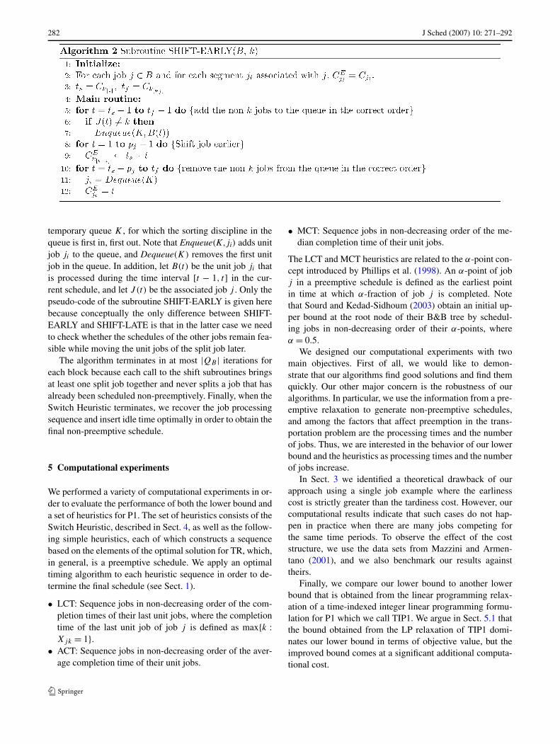
The two subroutines of the Switch Heuristic, SHIFT-EARLY and SHIFT-LATE, shift a job adjacent to its ear-liest unit job, or its latest unit job, respectively. We define a

282 J Sched (2007) 10: 271–292

temporary queue K , for which the sorting discipline in thequeue is first in, first out. Note that Enqueue(K, ji) adds unitjob ji to the queue, and Dequeue(K) removes the first unitjob in the queue. In addition, let B(t) be the unit job ji thatis processed during the time interval [t − 1, t] in the cur-rent schedule, and let J (t) be the associated job j . Only thepseudo-code of the subroutine SHIFT-EARLY is given herebecause conceptually the only difference between SHIFT-EARLY and SHIFT-LATE is that in the latter case we needto check whether the schedules of the other jobs remain fea-sible while moving the unit jobs of the split job later.

The algorithm terminates in at most |QB | iterations foreach block because each call to the shift subroutines bringsat least one split job together and never splits a job that hasalready been scheduled non-preemptively. Finally, when theSwitch Heuristic terminates, we recover the job processingsequence and insert idle time optimally in order to obtain thefinal non-preemptive schedule.

5 Computational experiments

We performed a variety of computational experiments in or-der to evaluate the performance of both the lower bound anda set of heuristics for P1. The set of heuristics consists of theSwitch Heuristic, described in Sect. 4, as well as the follow-ing simple heuristics, each of which constructs a sequencebased on the elements of the optimal solution for TR, which,in general, is a preemptive schedule. We apply an optimaltiming algorithm to each heuristic sequence in order to de-termine the final schedule (see Sect. 1).

• LCT: Sequence jobs in non-decreasing order of the com-pletion times of their last unit jobs, where the completiontime of the last unit job of job j is defined as max{k :Xjk = 1}.

• ACT: Sequence jobs in non-decreasing order of the aver-age completion time of their unit jobs.

• MCT: Sequence jobs in non-decreasing order of the me-dian completion time of their unit jobs.

The LCT and MCT heuristics are related to the α-point con-cept introduced by Phillips et al. (1998). An α-point of jobj in a preemptive schedule is defined as the earliest pointin time at which α-fraction of job j is completed. Notethat Sourd and Kedad-Sidhoum (2003) obtain an initial up-per bound at the root node of their B&B tree by schedul-ing jobs in non-decreasing order of their α-points, whereα = 0.5.

We designed our computational experiments with twomain objectives. First of all, we would like to demon-strate that our algorithms find good solutions and find themquickly. Our other major concern is the robustness of ouralgorithms. In particular, we use the information from a pre-emptive relaxation to generate non-preemptive schedules,and among the factors that affect preemption in the trans-portation problem are the processing times and the numberof jobs. Thus, we are interested in the behavior of our lowerbound and the heuristics as processing times and the numberof jobs increase.

In Sect. 3 we identified a theoretical drawback of ourapproach using a single job example where the earlinesscost is strictly greater than the tardiness cost. However, ourcomputational results indicate that such cases do not hap-pen in practice when there are many jobs competing forthe same time periods. To observe the effect of the coststructure, we use the data sets from Mazzini and Armen-tano (2001), and we also benchmark our results againsttheirs.

Finally, we compare our lower bound to another lowerbound that is obtained from the linear programming relax-ation of a time-indexed integer linear programming formu-lation for P1 which we call TIP1. We argue in Sect. 5.1 thatthe bound obtained from the LP relaxation of TIP1 domi-nates our lower bound in terms of objective value, but theimproved bound comes at a significant additional computa-tional cost.

J Sched (2007) 10: 271–292 283

5.1 Another lower bound

It is well known that the LP relaxations of time-indexed in-teger linear programming formulations of single machinescheduling problems, first introduced by Dyer and Wolsey(1990), provide very tight bounds. In this section, we ar-gue that the lower bound obtained from the LP relaxationof TIP1 dominates the lower bound from TR. However, thetightness of the LP relaxation comes at a significant addi-tional computational cost, as we demonstrate in the com-putational experiments. The lower bound obtained from theLP relaxation of TIP1 is useful for instances that we couldnot solve to optimality. It allows us to compute a tight upperbound on the optimality gaps of our heuristic solutions insuch instances.

From Sects. 2 and 3, recall that tmin = minj rj + 1,tmax = maxj max(rj , dj ) + P , and the planning horizon isdefined as H = {k | k ∈ Z, k ∈ [tmin, tmax]}. In this section,let t

j

min = rj + pj . Also, define zjk as a binary variable thattakes the value 1 if job j finishes processing at time k, andzero, otherwise. Then the time-indexed formulation of P1 is:

(TIP1) min∑

j

∑

k∈H

k≥tjmin

zjk(εj (dj − k)+

+ πj (k − dj )+), (5.1)

∑

j

min(tmax,k+pj −1)∑

t=max(k,tjmin)

zjt ≤ 1, ∀k ∈ H, (5.2)

∑

k∈H

k≥tjmin

zjk = 1, ∀j, (5.3)

zjk ∈ {0,1}, ∀j, k ∈ H,k ≥ tj

min. (5.4)

The constraints (5.2) and (5.4) together prescribe that atmost one job is processed by the machine at any pointin time and that processing is non-preemptive. Constraints(5.3) ensure that all jobs are processed.

Now consider the linear programming relaxationLP(TIP1) of TIP1. A fractional value α for zjk implies thatjob j is processed on the machine in each of the pj unit-length time periods [k − pj , k − pj + 1], . . . , [k − 1, k], butonly for a fraction α in any such period. This implies thatLP(TIP1) is a more constrained version of TR that imposescontiguity constraints on Xjk’s that belong to the same job.By using this observation and Theorem 2.2, one can show

that for each feasible solution of LP(TIP1) there exists afeasible solution for TR with no greater objective functionvalue. Thus, LP(TIP1) provides a tighter bound than TR.Refer to Bülbül (2002) for a formal proof of Theorem 5.1.

Theorem 5.1 TC(S∗TR) ≤ TC(S∗

LP(TIP1)) ≤ TC(S∗P1).

5.2 Data generation

To generate the processing times and the due dates of jobsfor our computational study, we follow the popular schemeof Potts and van Wassenhove (1982). This method is mo-tivated by the observation that the mean and the range ofthe due date distribution determines the level of difficultyof scheduling problems with due dates (also, see Hall andPosner 2001).

Processing times are generated from a discrete uniformdistribution U [pmin,pmax]. Then, the due dates are gener-ated from a discrete uniform distribution U [(1 − TF −RDD

2 ) ∗ P �, (1 − TF + RDD2 ) ∗ P �], where P is the sum

of the processing times. The tardiness factor, TF, is a coarsemeasure of the proportion of jobs that might be expected tobe tardy in an arbitrary sequence (Srinivasan 1971), and thedue date range factor, RDD, specifies the width of the in-terval centered around the average due date from which thedue dates are generated. If 1−TF − RDD

2 < 0, then the lowerbound of the due date range is set to zero.

The ready times are generated from a discrete uniformdistribution U [0,P ]. The earliness and tardiness costs aregenerated from uniform distributions U [εmin, εmax] andU [πmin,πmax], respectively.

5.3 Summary of results

The solution procedure for TR and the heuristics are imple-mented in C using CPLEX 9.0 callable libraries. When-ever possible, TIP1 and/or its linear programming relaxationare solved by ILOG AMPL 9.0 and the solver CPLEX9.0. All computations are performed on a Sun Blade 1000workstation with 512 MB of memory. In the following sec-tions, we examine the effects of the number of jobs, process-ing times and the relationship between the earliness and tar-diness costs on the performance of our algorithms. We alsobenchmark our algorithms against results published in theliterature.

5.3.1 Number of jobs

In order to test whether increasing the number of jobs affectsthe performance of the lower bound and the heuristics, we

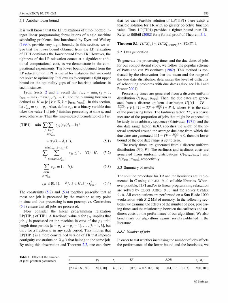
Table 1 Effect of the numberof jobs: problem parameters n pj rj TF RDD εj , πj

{20, 40, 60, 80} U [1,10] U [0,P ] {0.2, 0.4, 0.5, 0.6, 0.8} {0.4, 0.7, 1.0, 1.3} U [0,100]

284 J Sched (2007) 10: 271–292

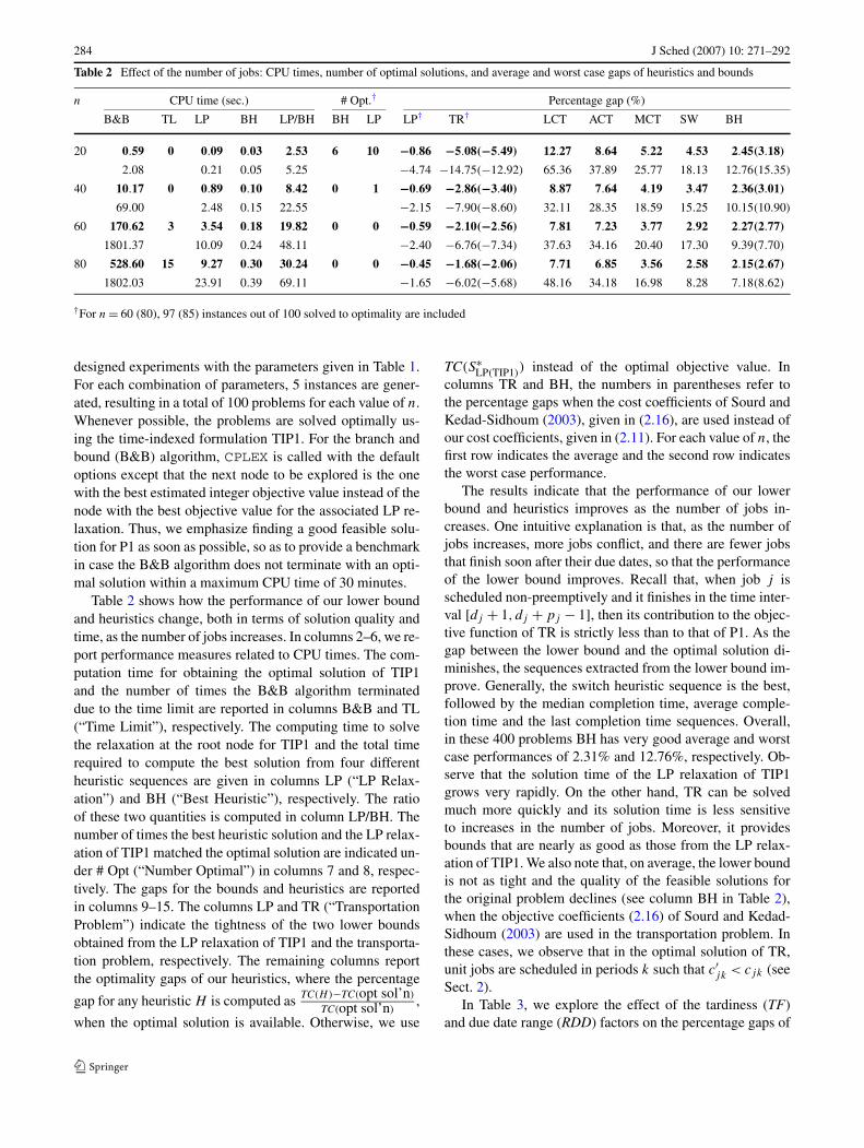
Table 2 Effect of the number of jobs: CPU times, number of optimal solutions, and average and worst case gaps of heuristics and bounds

n CPU time (sec.) # Opt.† Percentage gap (%)

B&B TL LP BH LP/BH BH LP LP† TR† LCT ACT MCT SW BH

20 0.59 0 0.09 0.03 2.53 6 10 −0.86 −5.08(−5.49) 12.27 8.64 5.22 4.53 2.45(3.18)

2.08 0.21 0.05 5.25 −4.74 −14.75(−12.92) 65.36 37.89 25.77 18.13 12.76(15.35)

40 10.17 0 0.89 0.10 8.42 0 1 −0.69 −2.86(−3.40) 8.87 7.64 4.19 3.47 2.36(3.01)

69.00 2.48 0.15 22.55 −2.15 −7.90(−8.60) 32.11 28.35 18.59 15.25 10.15(10.90)

60 170.62 3 3.54 0.18 19.82 0 0 −0.59 −2.10(−2.56) 7.81 7.23 3.77 2.92 2.27(2.77)

1801.37 10.09 0.24 48.11 −2.40 −6.76(−7.34) 37.63 34.16 20.40 17.30 9.39(7.70)

80 528.60 15 9.27 0.30 30.24 0 0 −0.45 −1.68(−2.06) 7.71 6.85 3.56 2.58 2.15(2.67)

1802.03 23.91 0.39 69.11 −1.65 −6.02(−5.68) 48.16 34.18 16.98 8.28 7.18(8.62)

†For n = 60 (80), 97 (85) instances out of 100 solved to optimality are included

designed experiments with the parameters given in Table 1.For each combination of parameters, 5 instances are gener-ated, resulting in a total of 100 problems for each value of n.Whenever possible, the problems are solved optimally us-ing the time-indexed formulation TIP1. For the branch andbound (B&B) algorithm, CPLEX is called with the defaultoptions except that the next node to be explored is the onewith the best estimated integer objective value instead of thenode with the best objective value for the associated LP re-laxation. Thus, we emphasize finding a good feasible solu-tion for P1 as soon as possible, so as to provide a benchmarkin case the B&B algorithm does not terminate with an opti-mal solution within a maximum CPU time of 30 minutes.

Table 2 shows how the performance of our lower boundand heuristics change, both in terms of solution quality andtime, as the number of jobs increases. In columns 2–6, we re-port performance measures related to CPU times. The com-putation time for obtaining the optimal solution of TIP1and the number of times the B&B algorithm terminateddue to the time limit are reported in columns B&B and TL(“Time Limit”), respectively. The computing time to solvethe relaxation at the root node for TIP1 and the total timerequired to compute the best solution from four differentheuristic sequences are given in columns LP (“LP Relax-ation”) and BH (“Best Heuristic”), respectively. The ratioof these two quantities is computed in column LP/BH. Thenumber of times the best heuristic solution and the LP relax-ation of TIP1 matched the optimal solution are indicated un-der # Opt (“Number Optimal”) in columns 7 and 8, respec-tively. The gaps for the bounds and heuristics are reportedin columns 9–15. The columns LP and TR (“TransportationProblem”) indicate the tightness of the two lower boundsobtained from the LP relaxation of TIP1 and the transporta-tion problem, respectively. The remaining columns reportthe optimality gaps of our heuristics, where the percentage

gap for any heuristic H is computed as TC(H)−TC(opt sol’n)

TC(opt sol’n),

when the optimal solution is available. Otherwise, we use

TC(S∗LP(TIP1)

) instead of the optimal objective value. Incolumns TR and BH, the numbers in parentheses refer tothe percentage gaps when the cost coefficients of Sourd andKedad-Sidhoum (2003), given in (2.16), are used instead ofour cost coefficients, given in (2.11). For each value of n, thefirst row indicates the average and the second row indicatesthe worst case performance.

The results indicate that the performance of our lowerbound and heuristics improves as the number of jobs in-creases. One intuitive explanation is that, as the number ofjobs increases, more jobs conflict, and there are fewer jobsthat finish soon after their due dates, so that the performanceof the lower bound improves. Recall that, when job j isscheduled non-preemptively and it finishes in the time inter-val [dj + 1, dj + pj − 1], then its contribution to the objec-tive function of TR is strictly less than to that of P1. As thegap between the lower bound and the optimal solution di-minishes, the sequences extracted from the lower bound im-prove. Generally, the switch heuristic sequence is the best,followed by the median completion time, average comple-tion time and the last completion time sequences. Overall,in these 400 problems BH has very good average and worstcase performances of 2.31% and 12.76%, respectively. Ob-serve that the solution time of the LP relaxation of TIP1grows very rapidly. On the other hand, TR can be solvedmuch more quickly and its solution time is less sensitiveto increases in the number of jobs. Moreover, it providesbounds that are nearly as good as those from the LP relax-ation of TIP1. We also note that, on average, the lower boundis not as tight and the quality of the feasible solutions forthe original problem declines (see column BH in Table 2),when the objective coefficients (2.16) of Sourd and Kedad-Sidhoum (2003) are used in the transportation problem. Inthese cases, we observe that in the optimal solution of TR,unit jobs are scheduled in periods k such that c′

jk < cjk (seeSect. 2).

In Table 3, we explore the effect of the tardiness (TF)and due date range (RDD) factors on the percentage gaps of

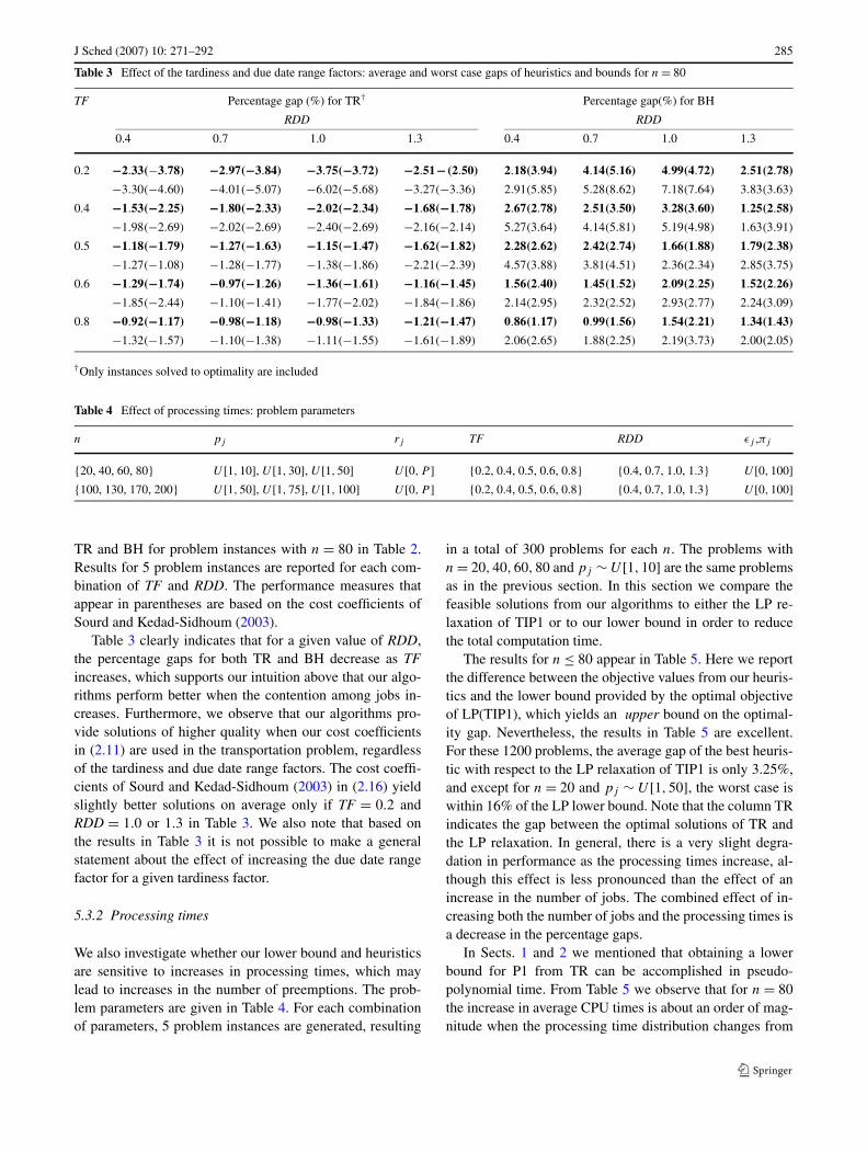
J Sched (2007) 10: 271–292 285

Table 3 Effect of the tardiness and due date range factors: average and worst case gaps of heuristics and bounds for n = 80

TF Percentage gap (%) for TR† Percentage gap(%) for BH

RDD RDD

0.4 0.7 1.0 1.3 0.4 0.7 1.0 1.3

0.2 −2.33(−3.78) −2.97(−3.84) −3.75(−3.72) −2.51−(2.50) 2.18(3.94) 4.14(5.16) 4.99(4.72) 2.51(2.78)

−3.30(−4.60) −4.01(−5.07) −6.02(−5.68) −3.27(−3.36) 2.91(5.85) 5.28(8.62) 7.18(7.64) 3.83(3.63)

0.4 −1.53(−2.25) −1.80(−2.33) −2.02(−2.34) −1.68(−1.78) 2.67(2.78) 2.51(3.50) 3.28(3.60) 1.25(2.58)

−1.98(−2.69) −2.02(−2.69) −2.40(−2.69) −2.16(−2.14) 5.27(3.64) 4.14(5.81) 5.19(4.98) 1.63(3.91)

0.5 −1.18(−1.79) −1.27(−1.63) −1.15(−1.47) −1.62(−1.82) 2.28(2.62) 2.42(2.74) 1.66(1.88) 1.79(2.38)

−1.27(−1.08) −1.28(−1.77) −1.38(−1.86) −2.21(−2.39) 4.57(3.88) 3.81(4.51) 2.36(2.34) 2.85(3.75)

0.6 −1.29(−1.74) −0.97(−1.26) −1.36(−1.61) −1.16(−1.45) 1.56(2.40) 1.45(1.52) 2.09(2.25) 1.52(2.26)

−1.85(−2.44) −1.10(−1.41) −1.77(−2.02) −1.84(−1.86) 2.14(2.95) 2.32(2.52) 2.93(2.77) 2.24(3.09)

0.8 −0.92(−1.17) −0.98(−1.18) −0.98(−1.33) −1.21(−1.47) 0.86(1.17) 0.99(1.56) 1.54(2.21) 1.34(1.43)

−1.32(−1.57) −1.10(−1.38) −1.11(−1.55) −1.61(−1.89) 2.06(2.65) 1.88(2.25) 2.19(3.73) 2.00(2.05)

†Only instances solved to optimality are included

Table 4 Effect of processing times: problem parameters

n pj rj TF RDD εj ,πj

{20, 40, 60, 80} U [1,10], U [1,30], U [1,50] U [0,P ] {0.2, 0.4, 0.5, 0.6, 0.8} {0.4, 0.7, 1.0, 1.3} U [0,100]{100, 130, 170, 200} U [1,50], U [1,75], U [1,100] U [0,P ] {0.2, 0.4, 0.5, 0.6, 0.8} {0.4, 0.7, 1.0, 1.3} U [0,100]

TR and BH for problem instances with n = 80 in Table 2.Results for 5 problem instances are reported for each com-bination of TF and RDD. The performance measures thatappear in parentheses are based on the cost coefficients ofSourd and Kedad-Sidhoum (2003).

Table 3 clearly indicates that for a given value of RDD,the percentage gaps for both TR and BH decrease as TFincreases, which supports our intuition above that our algo-rithms perform better when the contention among jobs in-creases. Furthermore, we observe that our algorithms pro-vide solutions of higher quality when our cost coefficientsin (2.11) are used in the transportation problem, regardlessof the tardiness and due date range factors. The cost coeffi-cients of Sourd and Kedad-Sidhoum (2003) in (2.16) yieldslightly better solutions on average only if TF = 0.2 andRDD = 1.0 or 1.3 in Table 3. We also note that based onthe results in Table 3 it is not possible to make a generalstatement about the effect of increasing the due date rangefactor for a given tardiness factor.

5.3.2 Processing times

We also investigate whether our lower bound and heuristicsare sensitive to increases in processing times, which maylead to increases in the number of preemptions. The prob-lem parameters are given in Table 4. For each combinationof parameters, 5 problem instances are generated, resulting

in a total of 300 problems for each n. The problems withn = 20,40,60,80 and pj ∼ U [1,10] are the same problemsas in the previous section. In this section we compare thefeasible solutions from our algorithms to either the LP re-laxation of TIP1 or to our lower bound in order to reducethe total computation time.

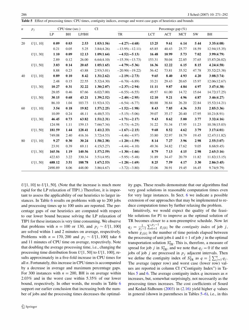
The results for n ≤ 80 appear in Table 5. Here we reportthe difference between the objective values from our heuris-tics and the lower bound provided by the optimal objectiveof LP(TIP1), which yields an upper bound on the optimal-ity gap. Nevertheless, the results in Table 5 are excellent.For these 1200 problems, the average gap of the best heuris-tic with respect to the LP relaxation of TIP1 is only 3.25%,and except for n = 20 and pj ∼ U [1,50], the worst case iswithin 16% of the LP lower bound. Note that the column TRindicates the gap between the optimal solutions of TR andthe LP relaxation. In general, there is a very slight degra-dation in performance as the processing times increase, al-though this effect is less pronounced than the effect of anincrease in the number of jobs. The combined effect of in-creasing both the number of jobs and the processing times isa decrease in the percentage gaps.

In Sects. 1 and 2 we mentioned that obtaining a lowerbound for P1 from TR can be accomplished in pseudo-polynomial time. From Table 5 we observe that for n = 80the increase in average CPU times is about an order of mag-nitude when the processing time distribution changes from

286 J Sched (2007) 10: 271–292

Table 5 Effect of processing times: CPU times, contiguity indices, average and worst case gaps of heuristics and bounds

n pj CPU time (sec.) CI Percentage gap (%)

LP BH LP/BH TR LCT ACT MCT SW BH

20 U [1,10] 0.09 0.03 2.53 1.03(1.56) −4.27(−4.68) 13.25 9.61 6.14 5.44 3.35(4.08)

0.21 0.05 5.25 3.84(4.26) −13.95(−12.11) 65.85 40.43 25.77 18.59 12.94(15.35)

U [1,30] 1.10 0.09 12.13 1.09(1.64) −4.52(−5.13) 16.48 10.99 5.73 7.02 3.99(4.79)

2.89 0.12 26.00 6.64(4.10) −15.39(−13.73) 153.31 50.04 22.85 37.65 15.87(26.02)

U [1,50] 3.03 0.14 20.65 1.05(1.65) −4.79(−5.36) 16.36 12.22 6.15 8.15 4.24(4.58)

8.88 0.23 43.88 2.93(3.01) −20.90(−19.22) 56.42 73.81 35.52 47.78 35.52(23.38)

40 U [1,10] 0.89 0.10 8.42 1.31(2.62) −2.19(−2.73) 9.65 8.40 4.93 4.20 3.08(3.74)

2.48 0.15 22.55 5.32(4.30) −6.70(−6.89) 33.21 29.43 20.65 15.97 12.06(12.67)

U [1,30] 10.27 0.31 32.22 1.30(2.07) −2.37(−2.94) 11.11 9.87 4.84 4.97 3.47(4.38)

28.05 0.46 87.66 6.02(7.00) −6.55(−6.55) 49.57 61.00 14.72 15.64 14.72(17.25)

U [1,50] 30.15 0.68 43.21 1.39(2.52) −2.40(−2.95) 12.10 9.21 4.96 4.87 3.46(4.27)

86.10 1.04 103.73 11.92(4.32) −6.54(−6.77) 80.88 38.84 26.20 22.84 15.52(14.21)

60 U [1,10] 3.54 0.18 19.82 1.57(2.25) −1.52(−1.98) 8.43 7.85 4.36 3.51 2.85(3.36)

10.09 0.24 48.11 6.48(5.33) −5.15(−5.06) 39.07 35.17 20.40 17.95 10.21(8.91)

U [1,30] 46.45 0.73 63.82 1.51(2.31) −1.71(−2.17) 9.43 8.62 5.00 3.77 3.32(4.16)

124.98 1.11 159.13 7.66(7.34) −5.73(−6.25) 31.22 51.34 17.95 11.23 10.38(15.03)

U [1,50] 181.59 1.44 128.41 1.41(2.33) −1.67(−2.15) 9.68 8.52 4.62 3.79 3.17(4.01)

749.08 2.40 416.16 3.72(4.53) −4.46(−4.97) 33.80 32.97 18.79 19.45 12.47(11.82)

80 U [1,10] 9.27 0.30 30.24 1.58(2.38) −1.20(−1.59) 8.14 7.27 3.96 2.98 2.55(3.07)

23.91 0.39 69.11 4.15(5.27) −4.44(−4.10) 49.36 34.82 17.62 9.05 8.68(9.45)

U [1,30] 165.56 1.19 140.56 1.57(2.59) −1.30(−1.66) 8.79 7.13 4.15 2.98 2.65(3.16)

422.83 3.22 330.34 3.51(4.95) −5.95(−5.48) 31.89 34.47 20.79 11.82 11.82(13.15)

U [1,50] 688.12 3.51 188.78 1.67(2.53) −1.28(−1.69) 8.25 7.59 4.17 3.30 2.86(3.45)

2490.89 8.06 448.00 3.86(4.67) −3.72(−3.80) 33.06 38.91 19.45 16.45 9.74(9.79)

U [1,10] to U [1,50]. (Note that the increase is much morerapid for the LP relaxation of TIP1.) Therefore, it is impor-tant to assess the applicability of our heuristics to larger in-stances. In Table 6 results on problems with up to 200 jobsand processing times up to 100 units are reported. The per-centage gaps of our heuristics are computed with respectto our lower bound because solving the LP relaxation ofTIP1 for these instances is very time consuming. We observethat problems with n = 100 or 130, and pj ∼ U [1,100]are solved within 1 and 2 minutes on average, respectively.Problems with n = 170,200 and pj ∼ U [1,100] take 6and 11 minutes of CPU time on average, respectively. Notethat doubling the average processing time, i.e., changing theprocessing time distribution from U [1,50] to U [1,100], re-sults approximately in a five-fold increase in CPU times forall n. Fortunately, this increase in CPU times is accompaniedby a decrease in average and maximum percentage gaps.For 300 instances with n = 200, BH is on average within2.03% and in the worst case within 5.35% of our lowerbound, respectively. In other words, the results in Table 6support our earlier conclusion that increasing both the num-ber of jobs and the processing times decreases the optimal-

ity gaps. These results demonstrate that our algorithms findvery good solutions in reasonable computation times evenfor very large instances. In Sect. 6 we indicate a possibleextension of our approaches that may be implemented to re-duce computation times by further relaxing the problem.

Intuitively, we would expect the quality of the feasi-ble solutions for P1 to improve as the optimal solution ofTR becomes closer to a non-preemptive schedule. Now let

qj = 1pj −1

∑pj −1k=1 gj [k] be the contiguity index of job j ,

where gj [k] is the number of time periods elapsed betweenthe processing of unit jobs k and k+1 of job j in the optimaltransportation solution S∗

TR. This is, therefore, a measure ofspread for job j in S∗

TR, and we note that qj = 0 if the unitjobs of job j are processed in pj adjacent intervals. Thenwe define the contiguity index of S∗

TR as q = 1n

∑nj=1 qj .

The average (upper row) and worst case (lower row) val-ues are reported in column CI (“Contiguity Index”) in Ta-bles 5 and 6. The average contiguity index q increases as n

increases, but, somewhat surprisingly, not necessarily as theprocessing times increases. The cost coefficients of Sourdand Kedad-Sidhoum (2003) in (2.16) yield higher q valuesin general (shown in parentheses in Tables 5–6), i.e., in this

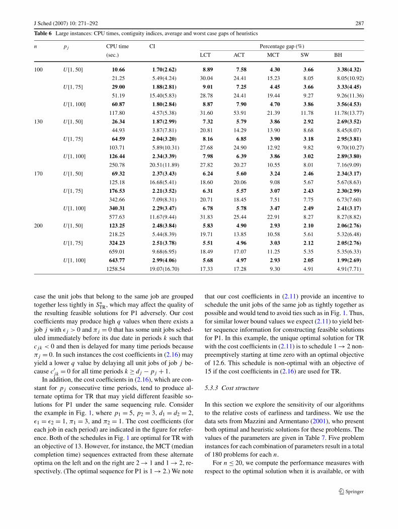
J Sched (2007) 10: 271–292 287

Table 6 Large instances: CPU times, contiguity indices, average and worst case gaps of heuristics

n pj CPU time CI Percentage gap (%)

(sec.) LCT ACT MCT SW BH

100 U [1,50] 10.66 1.70(2.62) 8.89 7.58 4.30 3.66 3.38(4.32)

21.25 5.49(4.24) 30.04 24.41 15.23 8.05 8.05(10.92)

U [1,75] 29.00 1.88(2.81) 9.01 7.25 4.45 3.66 3.33(4.45)

51.19 15.40(5.83) 28.78 24.41 19.44 9.27 9.26(11.36)

U [1,100] 60.87 1.80(2.84) 8.87 7.90 4.70 3.86 3.56(4.53)

117.80 4.57(5.38) 31.60 53.91 21.39 11.78 11.78(13.77)

130 U [1,50] 26.34 1.87(2.99) 7.32 5.79 3.86 2.92 2.69(3.52)

44.93 3.87(7.81) 20.81 14.29 13.90 8.68 8.45(8.07)

U [1,75] 64.59 2.04(3.20) 8.16 6.85 3.90 3.18 2.95(3.81)

103.71 5.89(10.31) 27.68 24.90 12.92 9.82 9.70(10.27)

U [1,100] 126.44 2.34(3.39) 7.98 6.39 3.86 3.02 2.89(3.80)

250.78 20.51(11.89) 27.82 20.27 10.55 8.01 7.16(9.09)

170 U [1,50] 69.32 2.37(3.43) 6.24 5.60 3.24 2.46 2.34(3.17)

125.18 16.68(5.41) 18.60 20.06 9.08 5.67 5.67(8.63)

U [1,75] 176.53 2.21(3.52) 6.31 5.57 3.07 2.43 2.30(2.99)

342.66 7.09(8.31) 20.71 18.45 7.51 7.75 6.73(7.60)

U [1,100] 340.31 2.29(3.47) 6.78 5.78 3.47 2.49 2.41(3.17)

577.63 11.67(9.44) 31.83 25.44 22.91 8.27 8.27(8.82)

200 U [1,50] 123.25 2.48(3.84) 5.83 4.90 2.93 2.10 2.06(2.76)

218.25 5.44(8.39) 19.71 13.85 10.58 5.61 5.32(6.48)

U [1,75] 324.23 2.51(3.78) 5.51 4.96 3.03 2.12 2.05(2.76)

659.01 9.68(6.95) 18.49 17.07 11.25 5.35 5.35(6.33)

U [1,100] 643.77 2.99(4.06) 5.68 4.97 2.93 2.05 1.99(2.69)

1258.54 19.07(16.70) 17.33 17.28 9.30 4.91 4.91(7.71)

case the unit jobs that belong to the same job are groupedtogether less tightly in S∗

TR, which may affect the quality ofthe resulting feasible solutions for P1 adversely. Our costcoefficients may produce high q values when there exists ajob j with εj > 0 and πj = 0 that has some unit jobs sched-uled immediately before its due date in periods k such thatcjk < 0 and then is delayed for many time periods becauseπj = 0. In such instances the cost coefficients in (2.16) mayyield a lower q value by delaying all unit jobs of job j be-cause c′

jk = 0 for all time periods k ≥ dj − pj + 1.In addition, the cost coefficients in (2.16), which are con-

stant for pj consecutive time periods, tend to produce al-ternate optima for TR that may yield different feasible so-lutions for P1 under the same sequencing rule. Considerthe example in Fig. 1, where p1 = 5, p2 = 3, d1 = d2 = 2,ε1 = ε2 = 1, π1 = 3, and π2 = 1. The cost coefficients (foreach job in each period) are indicated in the figure for refer-ence. Both of the schedules in Fig. 1 are optimal for TR withan objective of 13. However, for instance, the MCT (mediancompletion time) sequences extracted from these alternateoptima on the left and on the right are 2 → 1 and 1 → 2, re-spectively. (The optimal sequence for P1 is 1 → 2.) We note

that our cost coefficients in (2.11) provide an incentive toschedule the unit jobs of the same job as tightly together aspossible and would tend to avoid ties such as in Fig. 1. Thus,for similar lower bound values we expect (2.11) to yield bet-ter sequence information for constructing feasible solutionsfor P1. In this example, the unique optimal solution for TRwith the cost coefficients in (2.11) is to schedule 1 → 2 non-preemptively starting at time zero with an optimal objectiveof 12.6. This schedule is non-optimal with an objective of15 if the cost coefficients in (2.16) are used for TR.

5.3.3 Cost structure

In this section we explore the sensitivity of our algorithmsto the relative costs of earliness and tardiness. We use thedata sets from Mazzini and Armentano (2001), who presentboth optimal and heuristic solutions for these problems. Thevalues of the parameters are given in Table 7. Five probleminstances for each combination of parameters result in a totalof 180 problems for each n.

For n ≤ 20, we compute the performance measures withrespect to the optimal solution when it is available, or with

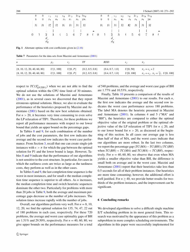
288 J Sched (2007) 10: 271–292

Fig. 1 Alternate optima with cost coefficients given in (2.16)

Table 7 Parameters for the data sets from Mazzini and Armentano (2001)

n pj rj TF RDD εj πj

{8, 10, 12, 20, 40, 60, 80} U [1,100] U [0,P ] {0.2, 0.5, 0.8} {0.4, 0.7, 1.0} U [0,50] πj = εj ∗ 2

{8, 10, 12, 20, 40, 60, 80} U [1,100] U [0,P ] {0.2, 0.5, 0.8} {0.4, 0.7, 1.0} U [0,100] πj = εj , πj = εj

2 , U [0,100]

respect to TC(S∗LP(TIP1)) when we are not able to find the

optimal solution within the CPU time limit of 30 minutes.We do not use the solutions of Mazzini and Armentano(2001), as in several cases we discovered that they reporterroneous optimal solutions. Hence, we also re-evaluate theperformance of the heuristics proposed by Mazzini and Ar-mentano (2001) based on the new best solutions obtained.For n > 20, it becomes very time consuming to even solvethe LP relaxation of TIP1. Therefore, for these problems wereport all performance measures with respect to our lowerbound that yields an upper bound on the percentage gaps.

In Tables 8 and 9, for each combination of the numberof jobs and the cost parameters, the first row indicates theaverage and the second row indicates the worst case perfor-mance. From Section 3, recall that one can create single-jobinstances with ε > π for which the gap between the optimalsolution for P1 and the lower bound is large. However, Ta-bles 8 and 9 indicate that the performance of our algorithmsis not sensitive to the cost structure. In particular, for cases inwhich the earliness costs are twice as large as the tardinesscosts, they perform as well as in the other cases.

In Tables 8 and 9, the last completion time sequence is theworst in most instances, and for small n the median comple-tion time sequence is superior to all others. As n increases,the median completion time and switch heuristic sequencesdominate the other two. Particularly for problems with morethan 20 jobs in Table 9, both the average and maximum per-centage gaps decrease as the number of jobs increases. Thesolution times increase rapidly with the number of jobs.

Overall, our algorithms perform very well. For n = 8, 10,12, 20, we find the optimal solution for 135, 74, 47, 22 outof 180 problems in each case, respectively. For these 720problems, the average and worst case optimality gaps of BHare 1.51% and 29.50%, respectively. For n = 40, 60, 80, wegive upper bounds on the performance measures for a total

of 540 problems, and the average and worst case gaps of BHare 1.77% and 10.53%, respectively.

Finally, Table 10 presents a comparison of the results ofMazzini and Armentano (2001) to our results. For each n,the first row indicates the average and the second row in-dicates the worst case performance across 180 problems.The label MA denotes the heuristic presented in Mazziniand Armentano (2001). In columns 4 and 5 (“MA” and“BH”), the heuristics are compared to either the optimalobjective value of the original problem or the optimal ob-jective value of the LP relaxation of TIP1 for n ≤ 20, andto our lower bound for n > 20, as discussed at the begin-ning of this section. In all cases our average gap is lessthan half of that of MA, and the worst cases indicate thatour algorithms are more robust. In the last two columns,we report the percentage gap (TC(MA)−TC(BH))/TC(BH)

when TC(BH) < TC(MA) and TC(MA) < TC(BH), respec-tively. For n = 40,60,80, we observe that even when MAyields a smaller objective value than BH, the difference issmall both on average and in the worst case. Mazzini andArmentano (2001) report that their heuristics take less than0.5 seconds for all of their problem instances. Our heuristicsare more time consuming; however, the additional effort iswell justified. For n ≥ 40, we provide better results for two-thirds of the problem instances, and the improvement can besignificant.

6 Concluding remarks

We developed algorithms to solve a difficult single machineE/T scheduling problem in its most general form. This re-search was motivated by the appearance of this problem as asubproblem in more complex scheduling environments. Thealgorithms in this paper were successfully implemented for

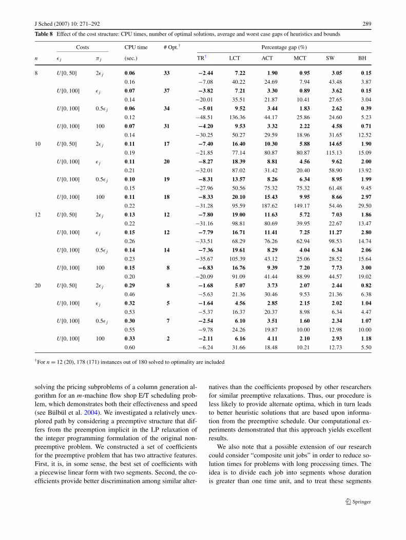
J Sched (2007) 10: 271–292 289

Table 8 Effect of the cost structure: CPU times, number of optimal solutions, average and worst case gaps of heuristics and bounds

Costs CPU time # Opt.† Percentage gap (%)

n εj πj (sec.) TR† LCT ACT MCT SW BH

8 U [0,50] 2εj 0.06 33 −2.44 7.22 1.90 0.95 3.05 0.15

0.16 −7.08 40.22 24.69 7.94 43.48 3.87

U [0,100] εj 0.07 37 −3.82 7.21 3.30 0.89 3.62 0.15

0.14 −20.01 35.51 21.87 10.41 27.65 3.04

U [0,100] 0.5εj 0.06 34 −5.01 9.52 3.44 1.83 2.62 0.39

0.12 −48.51 136.36 44.17 25.86 24.60 5.23

U [0,100] 100 0.07 31 −4.20 9.53 3.32 2.22 4.58 0.71

0.14 −30.25 50.27 29.59 18.96 31.65 12.52

10 U [0,50] 2εj 0.11 17 −7.40 16.40 10.30 5.88 14.65 1.90

0.19 −21.85 77.14 80.87 80.87 115.13 15.09

U [0,100] εj 0.11 20 −8.27 18.39 8.81 4.56 9.62 2.00

0.21 −32.01 87.02 31.42 20.40 58.90 13.92

U [0,100] 0.5εj 0.10 19 −8.31 13.57 8.26 6.34 8.95 1.99

0.15 −27.96 50.56 75.32 75.32 61.48 9.45

U [0,100] 100 0.11 18 −8.33 20.10 15.43 9.95 8.66 2.97

0.22 −31.28 95.59 187.62 149.17 54.46 29.50

12 U [0,50] 2εj 0.13 12 −7.80 19.00 11.63 5.72 7.03 1.86

0.22 −31.16 98.81 80.69 39.95 22.67 13.47

U [0,100] εj 0.15 12 −7.79 16.71 11.41 7.25 11.27 2.80

0.26 −33.51 68.29 76.26 62.94 98.53 14.74

U [0,100] 0.5εj 0.14 14 −7.36 19.61 8.29 4.04 6.34 2.06

0.23 −35.67 105.39 43.12 25.06 28.52 15.64

U [0,100] 100 0.15 8 −6.83 16.76 9.39 7.20 7.73 3.00

0.20 −20.09 91.09 41.44 88.99 44.57 19.02

20 U [0,50] 2εj 0.29 8 −1.68 5.07 3.73 2.07 2.44 0.82

0.46 −5.63 21.36 30.46 9.53 21.36 6.38

U [0,100] εj 0.32 5 −1.64 4.56 2.85 2.15 2.02 1.04

0.53 −5.37 16.37 20.37 8.98 6.34 4.47

U [0,100] 0.5εj 0.30 7 −2.54 6.10 3.51 1.60 2.34 1.07

0.55 −9.78 24.26 19.87 10.00 12.98 10.00

U [0,100] 100 0.33 2 −2.11 6.16 4.11 2.10 2.93 1.18

0.60 −6.24 31.66 18.48 10.21 12.73 5.50

†For n = 12 (20), 178 (171) instances out of 180 solved to optimality are included

solving the pricing subproblems of a column generation al-gorithm for an m-machine flow shop E/T scheduling prob-lem, which demonstrates both their effectiveness and speed(see Bülbül et al. 2004). We investigated a relatively unex-plored path by considering a preemptive structure that dif-fers from the preemption implicit in the LP relaxation ofthe integer programming formulation of the original non-preemptive problem. We constructed a set of coefficientsfor the preemptive problem that has two attractive features.First, it is, in some sense, the best set of coefficients witha piecewise linear form with two segments. Second, the co-efficients provide better discrimination among similar alter-

natives than the coefficients proposed by other researchersfor similar preemptive relaxations. Thus, our procedure isless likely to provide alternate optima, which in turn leadsto better heuristic solutions that are based upon informa-tion from the preemptive schedule. Our computational ex-periments demonstrated that this approach yields excellentresults.

We also note that a possible extension of our researchcould consider “composite unit jobs” in order to reduce so-lution times for problems with long processing times. Theidea is to divide each job into segments whose durationis greater than one time unit, and to treat these segments

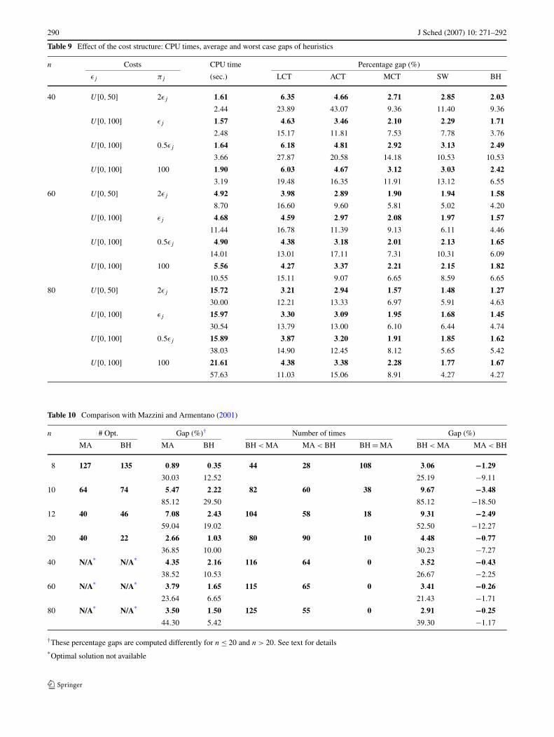
290 J Sched (2007) 10: 271–292

Table 9 Effect of the cost structure: CPU times, average and worst case gaps of heuristics

n Costs CPU time Percentage gap (%)

εj πj (sec.) LCT ACT MCT SW BH

40 U [0,50] 2εj 1.61 6.35 4.66 2.71 2.85 2.03

2.44 23.89 43.07 9.36 11.40 9.36

U [0,100] εj 1.57 4.63 3.46 2.10 2.29 1.71

2.48 15.17 11.81 7.53 7.78 3.76

U [0,100] 0.5εj 1.64 6.18 4.81 2.92 3.13 2.49

3.66 27.87 20.58 14.18 10.53 10.53

U [0,100] 100 1.90 6.03 4.67 3.12 3.03 2.42

3.19 19.48 16.35 11.91 13.12 6.55

60 U [0,50] 2εj 4.92 3.98 2.89 1.90 1.94 1.58

8.70 16.60 9.60 5.81 5.02 4.20

U [0,100] εj 4.68 4.59 2.97 2.08 1.97 1.57

11.44 16.78 11.39 9.13 6.11 4.46

U [0,100] 0.5εj 4.90 4.38 3.18 2.01 2.13 1.65

14.01 13.01 17.11 7.31 10.31 6.09

U [0,100] 100 5.56 4.27 3.37 2.21 2.15 1.82

10.55 15.11 9.07 6.65 8.59 6.65

80 U [0,50] 2εj 15.72 3.21 2.94 1.57 1.48 1.27

30.00 12.21 13.33 6.97 5.91 4.63

U [0,100] εj 15.97 3.30 3.09 1.95 1.68 1.45

30.54 13.79 13.00 6.10 6.44 4.74

U [0,100] 0.5εj 15.89 3.87 3.20 1.91 1.85 1.62

38.03 14.90 12.45 8.12 5.65 5.42

U [0,100] 100 21.61 4.38 3.38 2.28 1.77 1.67

57.63 11.03 15.06 8.91 4.27 4.27

Table 10 Comparison with Mazzini and Armentano (2001)

n # Opt. Gap (%)† Number of times Gap (%)

MA BH MA BH BH < MA MA < BH BH = MA BH < MA MA < BH

8 127 135 0.89 0.35 44 28 108 3.06 −1.29

30.03 12.52 25.19 −9.11

10 64 74 5.47 2.22 82 60 38 9.67 −3.48

85.12 29.50 85.12 −18.50

12 40 46 7.08 2.43 104 58 18 9.31 −2.49

59.04 19.02 52.50 −12.27

20 40 22 2.66 1.03 80 90 10 4.48 −0.77

36.85 10.00 30.23 −7.27

40 N/A* N/A* 4.35 2.16 116 64 0 3.52 −0.43

38.52 10.53 26.67 −2.25

60 N/A* N/A* 3.79 1.65 115 65 0 3.41 −0.26

23.64 6.65 21.43 −1.71

80 N/A* N/A* 3.50 1.50 125 55 0 2.91 −0.25

44.30 5.42 39.30 −1.17

†These percentage gaps are computed differently for n ≤ 20 and n > 20. See text for details*Optimal solution not available

J Sched (2007) 10: 271–292 291

in the same way as unit jobs are treated in our method-ology. This type of approximation can be implemented inmany different ways, but by experimenting with differ-ent values of the basic segment duration, one could tradeoff factors such as ease of constructing feasible solutionsfrom the solution of TR, solution quality and computingtime.

Our model is flexible and can be used to solve a varietyof problems by making appropriate adjustments to the prob-lem parameters. For instance, the weighted tardiness prob-lem can be solved by setting all earliness costs equal to zero.In addition, raw material inventory holding costs can eas-ily be incorporated for jobs that are ready, but waiting forprocessing by setting ε′

j = εj − hj and π ′j = πj + hj for

all jobs, where hj is the raw material inventory holding costof job j , and ε′

j and π ′j are the new earliness and tardiness

costs, respectively. We have already exploited this propertyto solve a flow shop scheduling problem with intermediateinventory holding costs (Bülbül et al. 2004), and hope toextend this research to job shop scheduling with inventoryholding costs in the future.

Acknowledgements We would like to thank Professor Vinicius Ar-mentano and Dr. Renata Mazzini for providing the data in Sect. 5.3.3.This research was partially supported by NSF Grant DMI-0092854.

References

Baker, K. R., & Scudder, G. D. (1990). Sequencing with earliness andtardiness penalties: a review. Operations Research, 38(1), 22–36.

Bülbül, K. (2002). Just-in-time scheduling with inventory holdingcosts. PhD thesis, University of California at Berkeley.

Bülbül, K., Kaminsky, P., & Yano, C. A. (2004). Flow shop schedulingwith earliness, tardiness and intermediate inventory holding costs.Naval Research Logistics, 51(3), 407–445.

Davis, J., & Kanet, J. (1993). Single-machine scheduling with earlyand tardy completion costs. Naval Research Logistics, 40(1), 85–101.

Dyer, M., & Wolsey, L. (1990). Formulating the single machine se-quencing problem with release dates as a mixed integer program.Discrete Applied Mathematics, 26(2–3), 255–270.

Fry, T., & Keong Leong, G. (1987). A bi-criterion approach to mini-mizing inventory costs on a single machine when early shipmentsare forbidden. Computers and Operations Research, 14(5), 363–368.

Fry, T., Armstrong, R., & Blackstone, J. (1987). Minimizing weightedabsolute deviation in single machine scheduling. IIE Transac-tions, 19(4), 445–450.

Fry, T., Armstrong, R., & Rosen, L. (1990). Single machine schedulingto minimize mean absolute lateness: a heuristic solution. Comput-ers and Operations Research, 17(1), 105–112.

Fry, T., Armstrong, R., Darby-Dowman, K., & Philipoom, P. (1996).A branch and bound procedure to minimize mean absolute late-ness on a single processor. Computers and Operations Research,23(2), 171–182.

Garey, M., Tarjan, R., & Wilfong, G. (1988). One-processor schedulingwith symmetric earliness and tardiness penalties. Mathematics ofOperations Research, 13(2), 330–348.

Gelders, L., & Kleindorfer, P. (1974). Coordinating aggregate and de-tailed scheduling decisions in the one-machine job shop, I: theory.Operations Research, 22(1), 46–60.

Graham, R., Lawler, E., Lenstra, J., & Rinnooy Kan, A. (1979). Op-timization and approximation in deterministic sequencing andscheduling: a survey. Annals of Discrete Mathematics, 5, 287–326.

Hall, N., & Posner, M. (2001). Generating experimental data for com-putational testing with machine scheduling applications. Opera-tions Research, 49(6), 854–865.

Hoogeveen, J., & van de Velde, S. (1996). A branch-and-bound algo-rithm for single-machine earliness-tardiness scheduling with idletime. INFORMS Journal on Computing, 8(4), 402–412.

Kanet, J., & Sridharan, V. (2000). Scheduling with inserted idle time:problem taxonomy and literature review. Operations Research,48(1), 99–110.

Kim, Y.-D., & Yano, C. A. (1994). Minimizing mean tardiness and ear-liness in single-machine scheduling problems with unequal duedates. Naval Research Logistics, 41(7), 913–933.

Lee, C., & Choi, J. (1995). A genetic algorithm for job sequencingproblems with distinct due dates and general early-tardy penaltyweights. Computers and Operations Research, 22(8), 857–869.

Lenstra, J., Rinnooy Kan, A., & Brucker, P. (1977). Complexity of ma-chine scheduling problems. Annals of Discrete Mathematics, 1,343–362.

Mazzini, R., & Armentano, V. (2001). A heuristic for single machinescheduling with early and tardy costs. European Journal of Oper-ational Research, 128(1), 129–146.

McNaughton, R. (1959). Scheduling with deadlines and loss functions.Management Science, 6(1), 1–12.

Mosheiov, G. (1996). A note on pre-emptive scheduling with earlinessand tardiness costs. Production Planning and Control, 7(4), 401–406.

Nandkeolyar, U., Ahmed, M., & Sundararaghavan, P. (1993). Dynamicsingle-machine-weighted absolute deviation problem: predictiveheuristics and evaluation. International Journal of Production Re-search, 31(6), 1453–1466.

Ovacik, I. M., & Uzsoy, R. (1997). Decomposition methods for com-plex factory scheduling problems. Boston: Kluwer Academic.

Phillips, C., Stein, C., & Wein, J. (1998). Minimizing average comple-tion time in the presence of release dates. Mathematical Program-ming, 82, 199–223.

Potts, C., & van Wassenhove, L. (1982). A decomposition algorithmfor the single machine total tardiness problem. Operations Re-search Letters, 1(5), 177–181.

Sourd, F. (2004). The continuous assignment problem and its appli-cation to preemptive and non-preemptive scheduling with irregu-lar cost functions. INFORMS Journal on Computing, 16(2), 198–208.

Sourd, F., & Kedad-Sidhoum, S. (2003). The one-machine problemwith earliness and tardiness penalties. Journal of Scheduling, 6(6),533–549.

Sridharan, V., & Zhou, Z. (1996). A decision theory based schedul-ing procedure for single-machine weighted earliness and tardi-ness problems. European Journal of Operational Research, 94(2),292–301.

Srinivasan, V. (1971). A hybrid algorithm for the one machine sequenc-ing problem to minimize total tardiness. Naval Research LogisticsQuarterly, 18(3), 317–327.

Szwarc, W. (1993). Adjacent orderings in single-machine schedulingwith earliness and tardiness penalties. Naval Research Logistics,40(2), 229–243.

Szwarc, W., & Mukhopadhyay, S. (1995). Optimal timing schedulesin earliness-tardiness single machine sequencing. Naval ResearchLogistics, 42(7), 1109–1114.

292 J Sched (2007) 10: 271–292

Ventura, J., & Radhakrishnan, S. (2003). Single machine schedulingwith symmetric earliness and tardiness penalties. European Jour-nal of Operational Research, 144(3), 598–612.

Verma, S., & Dessouky, M. (1998). Single-machine scheduling of unit-time jobs with earliness and tardiness penalties. Mathematics ofOperations Research, 23(4), 930–943.

Wan, G., & Yen, B. (2002). Tabu search for single machine schedulingwith distinct due windows and weighted earliness/tardiness penal-

ties. European Journal of Operational Research, 142(2), 271–281.

Yano, C. A., & Kim, Y. -D. (1991). Algorithms for a class of single-machine weighted tardiness and earliness problems. EuropeanJournal of Operational Research, 52(2), 167–178.