Predictive Analytics in Health Monitoring
174
Predictive Analytics in Health Monitoring by Alireza Manashty Master of Science, Shahrood University of Technology, Iran, 2012 Bachelor of Science, Razi University, Iran, 2010 A DISSERTATION SUBMITTED IN PARTIAL FULFILLMENT OF THE REQUIREMENTS FOR THE DEGREE OF Doctor of Philosophy (Ph.D.) In the Graduate Academic Unit of Computer Science Supervisor(s): Janet Light-Thompson, Ph.D., Dept. of Computer Science Examining Board: Suprio Ray, Ph.D., Faculty of Computer Science Huajie Zhang, Ph.D., Faculty of Computer Science Mary Ann Campbell, Ph.D., Dept. of Psychology External Examiner: Evangelos E. Milios, Ph.D., Faculty of Computer Science, Dalhousie University A dissertation is accepted by the Dean of Graduate Studies THE UNIVERSITY OF NEW BRUNSWICK February, 2019 Alireza Manashty, 2019
Transcript of Predictive Analytics in Health Monitoring

Predictive Analytics in Health Monitoring
by
Alireza Manashty
Master of Science, Shahrood University of Technology, Iran, 2012Bachelor of Science, Razi University, Iran, 2010
A DISSERTATION SUBMITTED IN PARTIAL FULFILLMENTOF THE REQUIREMENTS FOR THE DEGREE OF
Doctor of Philosophy (Ph.D.)
In the Graduate Academic Unit of Computer Science
Supervisor(s): Janet Light-Thompson, Ph.D., Dept. of Computer ScienceExamining Board: Suprio Ray, Ph.D., Faculty of Computer Science
Huajie Zhang, Ph.D., Faculty of Computer ScienceMary Ann Campbell, Ph.D., Dept. of Psychology
External Examiner: Evangelos E. Milios, Ph.D., Faculty of Computer Science,Dalhousie University
A dissertation is accepted by the
Dean of Graduate Studies
THE UNIVERSITY OF NEW BRUNSWICK
February, 2019
©Alireza Manashty, 2019

Abstract
Predictive analytics in healthcare can prevent patients emergency health con-
ditions and reduce costs in the long term. Accurate and timely anomaly pre-
dictions focusing on recent events can save lives. Nevertheless, for such ac-
curate predictions, machine learning algorithms require processing long-term
historical big data, which is infeasible in wearable devices due to their mem-
ory constraints and low computing power. Current techniques either ignore
a large amount of historical data or convert temporal sequences to pattern
sequences, eliminating valuable properties for prediction such as time and
recency. In addition, missing values in data collection can impair the predic-
tion. Hence, the motivation of this research is to efficiently model historical
data with missing values in a precise form of multivariate temporal sequences
to detect and forecast emergency events.
The proposed model is named as life model (LM). LM creates a new concise
sequence to represent the history and the future as an intensity temporal
sequence (ITS) tensor. LM maps arbitrary-length multivariate discrete time-
series data to another concise sequence, called multivariate interval sequence
ii

(MIS). ITS and MIS retain the original data properties such as time, recency,
and scale, without being much susceptible to missing values. Since long short-
term memory (LSTM) recurrent neural networks are proved to be effective
models for modeling sequence data, the LM algorithms and their properties
enable ITS and MIS tensors to train LSTM and other machine learning
techniques efficiently in order to predict in real-time, even in the absence of
some values.
LM is tested to predict and forecast emergency event such as the mortality
of a patient from the MIMIC III intensive care unit dataset. Based on their
diagnosis and procedure codes over a span of 11 years, the model achieved
84.2% and 99.6% accuracy on 34k and 10k patient records respectively.
In addition, the LM model is tested to predict the approximate time of
certain human activities, with different granularity of seconds and up even
to years. When tested on the URFD fall dataset, the experimental results
show that, compared to a previous study using a complex LSTM network,
LM achieves the same 100% accuracy in fall prediction using 80× less weight
parameters and computing power. LM is observed to forecast human fall up
to 14 seconds in advance with 86.96% accuracy with all available data and
85.56% accuracy with 50% missing values.
Finally, a new LM -powered predictive health analytics and real-time monitor-
ing schema (PHARMS) is developed which uses deep learning for predictive
analysis in a medical internet of things environment using wearable devices.
iii

Dedication
To the love of my life, Zahra. To our blossom, Pania. For all the days and
nights that I could not be with them.
To Professor Janet Light, my dearest supervisor, who always supported me
with her wisdom, experience, diligence, and patience.
iv

Acknowledgements
The authors would like to thank Microsoft Research for providing Microsoft
Azure cloud services for this research as part of the Azure for Research grant
program (2016-2018).
v

Table of Contents
Abstract ii
Dedication iv
Acknowledgments v
Table of Contents x
List of Tables xi
List of Figures xv
Abbreviations xvi
1 Introduction 1
1.1 Research Challenges in Modeling Medical History . . . . . . . 2
1.2 Research Question . . . . . . . . . . . . . . . . . . . . . . . . 7
1.3 Motivation and Main Contributions . . . . . . . . . . . . . . . 7
1.4 Thesis Road Map . . . . . . . . . . . . . . . . . . . . . . . . . 11
2 Background 12
vi

2.1 Time Modeling . . . . . . . . . . . . . . . . . . . . . . . . . . 13
2.2 Temporal Data Modeling . . . . . . . . . . . . . . . . . . . . . 14
2.3 Detection, Prediction, and Forecasting . . . . . . . . . . . . . 18
2.4 Temporal Sequence Modeling . . . . . . . . . . . . . . . . . . 19
2.5 Deep Learning . . . . . . . . . . . . . . . . . . . . . . . . . . . 21
2.5.1 Recurrent Neural Networks (RNN) . . . . . . . . . . . 21
2.5.2 Long Short-Term Memory (LSTM) . . . . . . . . . . . 22
2.6 Summary . . . . . . . . . . . . . . . . . . . . . . . . . . . . . 22
3 Health Monitoring Systems 24
3.1 Predictive health monitoring . . . . . . . . . . . . . . . . . . . 26
3.2 Data Fusion . . . . . . . . . . . . . . . . . . . . . . . . . . . . 29
3.3 Ambient-Assisted Living (AAL) . . . . . . . . . . . . . . . . . 31
3.3.1 Context Awareness . . . . . . . . . . . . . . . . . . . . 32
3.3.2 Knowledge Sharing . . . . . . . . . . . . . . . . . . . . 33
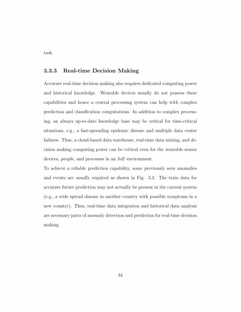
3.3.3 Real-time Decision Making . . . . . . . . . . . . . . . . 34
3.3.4 Efficient Service Delivery . . . . . . . . . . . . . . . . . 35
3.3.5 Comprehensive Monitoring System . . . . . . . . . . . 35
3.4 Existing Frameworks . . . . . . . . . . . . . . . . . . . . . . . 37
3.4.1 AAL-based Frameworks . . . . . . . . . . . . . . . . . 37
3.4.2 Cloud Prediction platforms . . . . . . . . . . . . . . . 39
3.5 Roadblocks . . . . . . . . . . . . . . . . . . . . . . . . . . . . 40
3.5.1 Policies, Privacy, and Trust . . . . . . . . . . . . . . . 41
vii

3.5.2 Security . . . . . . . . . . . . . . . . . . . . . . . . . . 42
3.5.3 Scalability . . . . . . . . . . . . . . . . . . . . . . . . . 43
3.6 Research Trends in internet of everything (IoE) Knowledge
Sharing Platforms . . . . . . . . . . . . . . . . . . . . . . . . . 44
3.7 Summary . . . . . . . . . . . . . . . . . . . . . . . . . . . . . 45
4 Health Data Representation for Predictive Analytics 46
4.1 Related Works in Health Data Representation . . . . . . . . . 46
4.2 Data Representation Taxonomy . . . . . . . . . . . . . . . . . 51
4.3 Current Techniques . . . . . . . . . . . . . . . . . . . . . . . . 52
4.4 Summary . . . . . . . . . . . . . . . . . . . . . . . . . . . . . 56
5 Life Model 57
5.1 Introduction . . . . . . . . . . . . . . . . . . . . . . . . . . . . 57
5.2 Life Model Definitions . . . . . . . . . . . . . . . . . . . . . . 60
5.2.1 Life Model for Time-series . . . . . . . . . . . . . . . . 60
5.2.2 Life Model for Multivariate State Sequences . . . . . . 65
5.3 LM Properties . . . . . . . . . . . . . . . . . . . . . . . . . . 72
5.3.1 Unit of time . . . . . . . . . . . . . . . . . . . . . . . . 72
5.3.2 Compression Ratio δ . . . . . . . . . . . . . . . . . . . 72
5.4 Prediction and Forecasting using Life Model . . . . . . . . . . 74
5.5 Evaluation and Loss Metrics . . . . . . . . . . . . . . . . . . . 76
5.6 Applications . . . . . . . . . . . . . . . . . . . . . . . . . . . . 78
5.7 Summary . . . . . . . . . . . . . . . . . . . . . . . . . . . . . 81
viii
6 Life Model Case Studies 82
6.1 Introduction . . . . . . . . . . . . . . . . . . . . . . . . . . . . 82
6.2 Test Metrics . . . . . . . . . . . . . . . . . . . . . . . . . . . . 83
6.3 Test Datasets . . . . . . . . . . . . . . . . . . . . . . . . . . . 84
6.4 Mortality Models . . . . . . . . . . . . . . . . . . . . . . . . . 87
6.4.1 Mortality Forecasting . . . . . . . . . . . . . . . . . . . 87
6.4.2 Mortality Detection . . . . . . . . . . . . . . . . . . . . 89
6.4.3 Diagnosis and Procedures Forecasting . . . . . . . . . . 93
6.4.4 Discussion . . . . . . . . . . . . . . . . . . . . . . . . . 94
6.5 Human Fall Prediction and Forecasting . . . . . . . . . . . . . 96
6.5.1 Introduction . . . . . . . . . . . . . . . . . . . . . . . . 96
6.5.2 Hardware Considerations . . . . . . . . . . . . . . . . . 97
6.5.3 Models . . . . . . . . . . . . . . . . . . . . . . . . . . . 99
6.5.3.1 Binary Prediction . . . . . . . . . . . . . . . . 99
6.5.4 Fall Forecasting . . . . . . . . . . . . . . . . . . . . . . 101
6.5.5 Fall Forecasting with Missing Values . . . . . . . . . . 102
6.6 Comparison with Recent Temporal Patterns (RTPs) . . . . . . 102
6.6.1 Simulated Data . . . . . . . . . . . . . . . . . . . . . . 103
6.6.2 Prediction Model . . . . . . . . . . . . . . . . . . . . . 104
6.6.3 Results and Comparison . . . . . . . . . . . . . . . . . 105
6.6.4 Discussion . . . . . . . . . . . . . . . . . . . . . . . . . 107
6.7 Human Activity Forecasting . . . . . . . . . . . . . . . . . . . 108
6.7.1 Forecasting Model . . . . . . . . . . . . . . . . . . . . 108
ix

6.7.2 Results . . . . . . . . . . . . . . . . . . . . . . . . . . . 109
6.7.3 Discussion . . . . . . . . . . . . . . . . . . . . . . . . . 109
6.8 Summary . . . . . . . . . . . . . . . . . . . . . . . . . . . . . 111
7 Predictive Health Analytics and Real-time Monitoring Schema
(PHARMS) 114
7.1 Introduction . . . . . . . . . . . . . . . . . . . . . . . . . . . . 114
7.2 Schema . . . . . . . . . . . . . . . . . . . . . . . . . . . . . . 116
7.3 Health Event Aggregation Lab (HEAL) . . . . . . . . . . . . . 117
7.3.1 Aggregators . . . . . . . . . . . . . . . . . . . . . . . . 120
7.3.2 Predictors . . . . . . . . . . . . . . . . . . . . . . . . . 122
7.4 Case Studies . . . . . . . . . . . . . . . . . . . . . . . . . . . . 124
7.4.1 Remote Dialysis . . . . . . . . . . . . . . . . . . . . . . 124
7.4.2 Mortality Prediction API . . . . . . . . . . . . . . . . . 127
7.4.3 Fall Forecasting Mobile App . . . . . . . . . . . . . . . 128
7.5 Summary . . . . . . . . . . . . . . . . . . . . . . . . . . . . . 128
8 Conclusion and Future Work 129
Bibliography 149
Vita
x

List of Tables
6.1 Mortality forecasting results using different metrics modeled
as LM period index as outcome. . . . . . . . . . . . . . . . . . 88
6.2 Accuracy, area under receiver operating characteristic (Au-
ROC), and Brier score for LM versus fixed-sized periods map-
pings for Mortality Prediction. . . . . . . . . . . . . . . . . . . 91
6.3 Comparison between LM and previous work on dataset. . . . 100
6.4 Performance of the LM and fixed size periods for fall prediction101
6.5 Fall forecast results for up to 14 seconds with various metrics
and levels of missing values. . . . . . . . . . . . . . . . . . . . 102
6.6 Accuracy (Average Recall) results for 10,000 patients using
different techniques. . . . . . . . . . . . . . . . . . . . . . . . . 106
6.7 Accuracy (Average Recall) results for 100,000 patients using
different techniques. . . . . . . . . . . . . . . . . . . . . . . . . 106
6.8 Accuracy and loss for LM versus fixed-size periods mappings
for activity recognition. . . . . . . . . . . . . . . . . . . . . . . 109
6.9 Comparison summary among LM and other techniques. . . . 112
xi

List of Figures
1.1 Sequence length per sample for a variety of sensory data for
specific time periods. . . . . . . . . . . . . . . . . . . . . . . 3
1.2 How fixed-length representations (b) of variable-length tem-
poral records (a) can create a meaningful input for different
learning algorithms in order to provide a better prediction. . 9
1.3 An example of how deep learning and LM -powered PHARMS
can create a minimally-invasive, intelligent remote monitoring,
and prediction platform using regular cameras only. . . . . . . 10
1.4 Remote dialysis assessment case study. . . . . . . . . . . . . . 11
2.1 Comparing multivariate temporal health data and time-series
techniques for forecasting. . . . . . . . . . . . . . . . . . . . . 13
2.2 Trend and value abstractions for creatinine values over time . 15
2.3 Several possible architectures of an recurrent neural network
(RNN). . . . . . . . . . . . . . . . . . . . . . . . . . . . . . . 19
2.4 It is often too late to detect an emergency event . . . . . . . . 20
2.5 Forecasting based on mapping from history . . . . . . . . . . . 20
2.6 RNN diagram . . . . . . . . . . . . . . . . . . . . . . . . . . . 23
xii

2.7 LSTM diagram . . . . . . . . . . . . . . . . . . . . . . . . . . 23
3.1 Joint directors of laboratories (JDL) model levels . . . . . . . 30
3.2 How remote monitoring systems work in an ambient-assisted
living (AAL) environment. . . . . . . . . . . . . . . . . . . . . 31
3.3 How predicting future trends and anomalies require train data
from past events. . . . . . . . . . . . . . . . . . . . . . . . . . 35
3.4 Predicting an anomaly with the help of an intelligent detection
and prediction system. . . . . . . . . . . . . . . . . . . . . . . 36
3.5 AAL Spaces and AAL Platforms interaction. . . . . . . . . . . 38
3.6 Fleet Management system demo utilizing Microsoft internet
of things (IoT) suite. . . . . . . . . . . . . . . . . . . . . . . . 41
4.1 Hand-engineering and combining different techniques to model
health data by Forkan et al. . . . . . . . . . . . . . . . . . . . 47
4.2 Recent temporal pattern (RTP) with a minimum gap by Iyad
et al. . . . . . . . . . . . . . . . . . . . . . . . . . . . . . . . . 49
4.3 Number of patients that had at least one admission in the last
year . . . . . . . . . . . . . . . . . . . . . . . . . . . . . . . . 52
4.4 An illustration of how an actual health dataset look like . . . 54
4.5 First approach for data modeling is to fill-in the missing values
with zeros . . . . . . . . . . . . . . . . . . . . . . . . . . . . . 54
4.6 Second approach for data modeling is to use none, but the
most recent data . . . . . . . . . . . . . . . . . . . . . . . . . 55
xiii

4.7 Third approach for data modeling is to remove the gaps (the
missing data) to create short sequences . . . . . . . . . . . . . 55
5.1 How LM models the data. . . . . . . . . . . . . . . . . . . . . 60
5.2 An example of LM mapping . . . . . . . . . . . . . . . . . . . 68
5.3 Relative position of temporal states. . . . . . . . . . . . . . . . 70
5.4 The effect of different values of time unit and δ on fill rate and
n. . . . . . . . . . . . . . . . . . . . . . . . . . . . . . . . . . . 73
5.5 LM mapping diagram for history and future. . . . . . . . . . . 74
5.6 The heatmap for mean squared error (MSE) versus tolerance
error (TE). . . . . . . . . . . . . . . . . . . . . . . . . . . . . 79
6.1 How forecasting data is prepared . . . . . . . . . . . . . . . . 87
6.2 Training and testing plots for mortality prediction on medical
information mart for intensive care (MIMIC) III dataset. . . . 92
6.3 The boxplot for mean tolerance error (MTE). . . . . . . . . . 95
6.4 Training and validation set accuracy and loss function plots of
activity prediction. . . . . . . . . . . . . . . . . . . . . . . . . 110
7.1 PHARMS , health event aggregation lab (HEAL), and the 3-
tier LM engine architectures. . . . . . . . . . . . . . . . . . . 118
7.2 HEAL Architecture . . . . . . . . . . . . . . . . . . . . . . . 119
7.3 An overview of HEAL framework. . . . . . . . . . . . . . . . . 121
7.4 Proposed aggregator model for HEAL. . . . . . . . . . . . . . 122
7.5 Proposed predictor model for HEAL platform . . . . . . . . . 123
xiv

7.6 HEAL core framework, an implementation of the HEAL ar-
chitecture. . . . . . . . . . . . . . . . . . . . . . . . . . . . . . 125
7.7 Four stages of the remote dialysis assessment study using HEAL
framework. . . . . . . . . . . . . . . . . . . . . . . . . . . . . . 127
xv
List of Abbreviations
AAL ambient-assisted living xiii, 24, 26–28, 30, 31, 37, 38, 46, 47, 116
ACM association for computing machinery 102
AIaaS artificial intelligence as a service 128
API application programming interface 40, 128
AuROC area under receiver operating characteristic xi, 48, 83, 91, 92, 100,
101
BSN body sensor network 120
CDSS clinical decision support system 115
CEP complex event processing 119, 126
CN2 CN2 algorithm 101
CNN convolutional neural network 98
CNTK Microsoft cognitive toolkit 104, 105, 108
xvi

CoCaMAAL cloud-oriented context-aware middleware in ambient assisted
living 25, 37, 38, 45, 46
DDSS diagnosis decision support system 115
DFF deep feed-forward neural network 105–108
ECG electrocardiography 27, 30, 120
EEG electroencephalography 27, 30, 120
EHR electronic health record 48
EMG electromyography 120
EMS emergency medical services 31
FN false negatives 83, 127
FP false positives 83
GBM gradient boosting machine 105–108
GMM generalized method of moments 48
GPU graphics processing unit 21, 90, 91, 94
HEAL health event aggregation lab xiv, xv, 25, 37, 43, 45, 114, 116–125,
127
HMM hidden Markov model 19, 47
xvii

HTTPS hypertext transfer protocol secure 42
Hz hertz 4, 86, 99, 108
ICA independent component analysis 48
ICD international classification of diseases 6, 14, 16, 49, 85, 89, 90
ICU intensive care unit 1, 6, 12–14
INR international normalized ratio 126
IoE internet of everything viii, 24–28, 30, 34–36, 39, 40, 42–45
IoMT internet of medical things 2, 40, 50
IoT internet of things xiii, 2, 6, 9, 10, 12, 39–43, 94, 118, 125, 129, 130
ITS intensity temporal sequence ii, iii, 8, 49, 59, 65–69, 71–74, 102, 105–108,
129
JDL joint directors of laboratories xiii, 29, 30
LM life model ii, iii, viii, xi, xii, xiv, 8–11, 22, 50, 56, 57, 59–63, 65, 66, 68,
71–78, 81, 83, 84, 86–94, 99–102, 108–114, 116, 118, 128–131
LMts life model for timeseries 59, 100–102
LR linear regression 14, 101
LSTM long short-term memory iii, xiii, 8, 18, 21–23, 48–53, 60, 74, 83, 88,
90, 91, 94, 97, 99–101, 104–108, 112, 129
xviii

MIMIC medical information mart for intensive care iii, xiv, 6, 14, 85, 87,
89, 92, 130
MIS multivariate interval sequence ii, iii, 8, 59, 61, 64, 65, 72–75, 78, 90,
92, 97, 98, 108, 110, 112, 129
MLP multilayer perceptron 48
MSE mean squared error xiv, 76, 79, 84, 88, 93, 95, 102
MSS multivariate state sequences 17, 51, 54, 59, 65–69, 71, 74
MTAS multivariate temporal abstraction sequence 103, 104
MTE mean tolerance error xiv, 77, 78, 84, 93–95
MTS multivariate temporal sequence 59–61, 64, 65, 74, 93
MVC model-view-controller 118
NB naiive bayes 101
NBHRF New Brunswick health research conference 124
NFC near-field communication 32
NHS National Health Service 52
OSGi open services gateway initiative 37
PaaS platform as a service 33, 39, 118
xix

PCA principle component analysis 48
PHARMS predictive health analytics and real-time monitoring schema iii,
xii, xiv, 9–11, 114–118, 124, 127, 128, 130
PI pattern injector 104
PIPEDA personal information protection and electronic documents act 41
PIR pattern injection rate 104
PR patient record 103, 104
RF random forests 101, 105, 106, 108
RFID radio-frequency identification 27, 32
RGB-D red-green-blue-depth 32
RNN recurrent neural network xii, 8, 18, 19, 21–23, 48, 50, 64, 65, 68, 81,
97, 98, 104, 108, 111, 112
ROC receiver operating characteristic 83, 91, 92
RTP recent temporal pattern xiii, 15, 49, 66, 102, 105–107, 111, 112
SaaS software as a service 114, 118
SDA stack of denoising autoencoders 48
Seq2Seq sequence to sequence 75–77
xx

SSL secure socket layer 42
SVM support vector machines 49, 101
TE tolerance error xiv, 76, 77, 79, 84, 88, 101, 102
TN true negatives 83
ToF time-of-flight 30
TP true positives 83
UI user-interface xiv, 119
URFD University of Rzeszow fall dataset 86, 99, 101
VM virtual machine 94
xxi

Chapter 1
Introduction
Predictive analytics in healthcare can prevent patients having emergency
health conditions, save lives, and reduce the cost of healthcare in the long
term. The USA budget for healthcare in 2017 was just over a trillion dollars
[1]. A 2012 study [2] showed that 61% of acute hospital patients experience
discharge delay, which causes delays for other patients, raises the costs, and
increases patient admission complications due to lack of emergency symptom
monitoring. In July 2017, a cohort Canadian study [3] showed that dying
risk for patients experiencing emergency surgery delay is 4.9% compared
with 3.2% for those without delay. Hence, predictive analytics plays an
important role in improving healthcare processes. Recently, researchers have
developed tools to predict hospital readmission rates [4], mortality risks in
the hospitals and particularly in the intensive care units (ICUs), and assign
severity scores to patients [5, 6]. The next step in this trend is disease
1

diagnosis and anomaly prediction, by which the hospital information system
can automatically identify a patient’s diagnosis code and forecast a disease
quickly and accurately in real-time for an emergency medical situation.
With the emerging internet of medical things (IoMT), modeling long his-
torical temporal health records for a patient with missing data is a major
challenge for predictive analytics. IoMT is a network of medical internet of
things (IoT) devices connected to the healthcare ecosystem. Recent studies
are using deep learning and data abstraction techniques to model health data
in such an environment [7, 8, 9]. However, it is difficult to train a model to
predict anomalies based on temporal sparse data. Specifically, representing
more than few seconds of an individual’s medical history in a short, con-
cise sequence is the keystone challenge for training deep learning algorithms.
Moreover, despite the missing data, the model should be robust and preserve
the concept of time and recency for a variety of samples, which is critical in
an IoMT environment.
1.1 Research Challenges in Modeling Medi-
cal History
To accurately predict the imminent health anomalies or events from real-
time medical history, it is necessary to properly model the long sequences
of an individual’s health and activity records. A temporal sequence is an
array of time-stamped records. For instance, family physician visits can be a
2

Figure 1.1: Sequence length per sample for a variety of sensory data forspecific time periods.
3

temporal sequence. If the interval between each record is a fixed value (e.g.,
every hour), the array is a time-series. An example of time-series data is
the recorded vital signs of a patient in a hospital bed. The problem with
using time-series modeling and activity recognition techniques for modeling
long periods of time is the length of the data and the presence of missing
data. Fig. 1.1 shows how long the sequence length of a single sample can be.
For example, accelerator sensor data for 3 days consists of approximately
13 million time-stamped records. The first step is usually discretizing the
real-time (continuous) data in order to create fewer time steps for easier pro-
cessing. In addition to discretization errors [10] in temporal data abstraction,
discrete value sequences obtained from historical medical data may require
missing value imputation first. Moreover, each data interval (short-term vs
long-term) generates a similar sequence length as any other interval in the
history. This similar sequence length causes one or both of the following
problems:
The resulting discretized sequences grow linearly as long as the medical
history is present. For example, if a person’s medical history for a day
is recorded at 50 hertz (Hz), 4.32 million records are recorded, which
exceeds the input dimension of many machine learning algorithms. Fig-
ure 1.1 illustrates this problem.
The above sequences are not the same for different patients with dif-
ferent available histories (length and quality of data). Patients do not
4

wear sensors 24/7, and even if they try to, such devices are unavailable
during charging. The resulting variation in sequence lengths (a few
seconds compared to hours, and days of data) makes it even harder (if
not impossible) to optimize a model for prediction.
Techniques are available [8] to create an abstract version of history by ex-
tracting patterns in data, which may ignore the missing values; however,
they are unable to produce an arbitrary length of history. A fixed concise
representation of history has many computational advantages. First, most
learning algorithms require fixed-size input. Even autoencoders, which can
create condensed representation of data, require a fixed input-length in the
first place. Furthermore, if a normalized representation implicitly handles
missing values, it can resolve a major challenge in sequence learning and
thus health prediction.
The summary of challenges addressed in this thesis are as follows:
Modeling long temporal sequences of sparse health data for
prediction
Modeling long-term sparse temporal data and training a machine learn-
ing model to properly benefit from critical dependencies, and distin-
guish that information from irrelevant noise, is an open problem. For
example, the hourly averages of 12 variables a day for 10 years, results
in an input sequence of more than one million records per patient. Fit-
ting decades of medical history, lifestyle, and activities into a concise
5

sequence—as to optimize machine learning—is a challenge.
Predicting patient mortality and diagnosis
There are many diagnostic classes for automated classification using
machine learning. In one of the largest datasets available (medical in-
formation mart for intensive care (MIMIC) III [11]), for around 40,000
patients in ICU , there are more than 15,000 unique international clas-
sification of diseases (ICD)-9 diagnosis codes defined by physicians.
At the first glance, we are facing a classification algorithm with 15,000
classes with fewer than 3 samples per class. For mortality prediction,
there are also more parameters to consider as most of the patient’s
data is based on hospital records—often only during the final admis-
sion process. With the help of medical IoT and real-time monitoring,
prediction can be extended to the patient’s day-to-day life rather than
only to the hospital visits.
Real-time health predictive analytics
An intelligent and practical system that can provide smart real-time
predictive health anomaly decision support for physicians and patients
is not yet available in the literature. Such a system should be able to
receive data from many IoT edge sensors, provide predictive analytics,
and send feedback in a timely manner.
6

1.2 Research Question
In this research we seek to answer the following question:
“How can temporal sequences be modeled to improve the analytic process in
real-time prediction?”
We divide the research problem further into three questions:
1. How can the multivariate sparse temporal data be modeled from an
individual’s lifetime medical records for the learning algorithms? More
specifically, how to model the data in such a way that both long-term
and short-term (and even real-time data) could be fed into the same
model for it to be able to predict events as accurate as possible?
2. Which learning algorithm fits the above model better?
3. What architecture/framework is best suited for the above purposes?
1.3 Motivation and Main Contributions
The main objective of this research is to address the challenges in the develop-
ment of a system that can provide predictive analytics for health monitoring.
Anomaly detection is not adequate for many scenarios as it may be already
too late to detect an emergency event. For example, in detection, we ask
the question: “Do I have cancer?” or “Has my father fallen today/now?”
whereas in forecasting/prediction, we ask: “Will I get cancer? When?” or
“Is it likely for my father to have an accident (fall) today?”. Finding the
7

answers to the above forecasting questions are more challenging than the
detection problem. The motivation of this research is to model long-term
temporal sequences—usually with missing values—to not only detect, but to
forecast events in either wearable deep learning hardware [12] or cloud-based
services.
In this research, a novel time-mapping model called Life model (LM) is pro-
posed for modeling temporal sequences to achieve a concise sequence of an
individual’s data records. (See Fig. 1.2). The LM provides an n-bit sequence
to represent the data in history or the future named as either an intensity tem-
poral sequence (ITS) or multivariate interval sequence (MIS) tensor1, based
on the type of input (explained in Chapter 5). LM algorithms and properties
enable these tensors to train machine learning models efficiently, especially
long short-term memory (LSTM) recurrent neural networks (RNNs).
The development and testing of the novel models, algorithms, processes, and
the architectures listed below to address the above challenges, are the main
contributions in this research:
1. A novel modeling of health records, activities, and future predictions
2. Temporal abstraction techniques for modeling long-term sparse multi-
variate temporal data for optimized learning
3. An architecture/framework for real-time health analytics
1In this thesis, ITS or MIS are vectors of tensors, and tensors can safely be assumedas multidimensional arrays in this document.
8

Binary Classification
Sequence to SequenceClassification/Regression
Life ModelMIS
Autoencoder
(a) Variable historical records with missing values
(b) Fixed-length representations
Mapping
Reducing Predicting FeedbackIndividuals' Records
Figure 1.2: How fixed-length representations (b) of variable-length temporalrecords (a) can create a meaningful input for different learning algorithms inorder to provide a better prediction.
The proposed LM -powered predictive health analytics and real-time moni-
toring schema (PHARMS) promises to provide a solution to improve pre-
dictive health analytics via IoT edge devices and wearables. It enables
real-time minimally-invasive intelligent activity monitoring and predictive
analysis based on various deep learning techniques. It is also the testbed for
evaluating the LM in a cloud environment, using real-world and simulated
data.
Testing with different scenarios show how smart health using real-time moni-
toring and predictive analysis can improve healthcare synergistically. Figure
1.3 shows how a remote patient monitoring system can use the LM -enabled
PHARMS to detect and predict anomalies to recover from an emergency
condition (here, it predicts a ‘fall’). The cloud-based backend provides ad-
9

Figure 1.3: An example of how deep learning and LM -powered PHARMScan create a minimally-invasive, intelligent remote monitoring, and predictionplatform using regular cameras only.
vanced intelligence to notify the caregivers in real-time. Figure 1.4 shows
another example of how a remote dialysis assessment system can benefit
from PHARMS to help renal patients avoid early/late visits to hospitals us-
ing a self-assessment device at home. Combined with real-time monitoring
and IoT , accidents such as falls, heart attacks, and seizures, can be pre-
vented with health anomaly prediction. Warning users of complications of a
drug, or providing early predictions of a disease, are among the many other
applications of PHARMS .
10

Figure 1.4: Remote dialysis assessment case study.
1.4 Thesis Road Map
In chapter 1, an overview of the challenges and research questions was dis-
cussed. Chapter 2 covers the background on time modeling, data abstrac-
tion, and deep learning, which is required to understand the rest of the thesis.
Chapter 3 reviews cloud-based health monitoring systems that are facilitat-
ing predictive analytics. Chapter 4 reviews related works in more depth and
covers the theoretical background for temporal modeling. Chapters 5 and 6
describe the proposed LM and its applications, including evaluation for var-
ious predictive test cases. Chapter 7 covers the proposed PHARMS schema
and Chapter 8 concludes the thesis.
11

Chapter 2
Background
Unlike a time-series with fixed intervals, health data is often collected spo-
radically. For instance, the patient visits a doctor and a medical record is
added; then a few months later there is another record, and then maybe no
records are added for a few years. Moreover, wearable devices are not always
worn and IoT edge devices are not always monitoring patients. In emergency
conditions, for patients in hospitals and ICUs , more tests are performed and
more data is available. However, even in hospitals, years of family and med-
ical history are summarized in a paragraph or two, making it challenging to
integrate with the rest of the data. In disease prediction and health mon-
itoring we are interested in temporal sequence data. Time-series modeling
techniques are not applicable for sparse medical temporal data sequences;
therefore, other prediction techniques should be used. Fig. 2.1 compares
time-series forecasting with multivariate temporal health data modeling.
12

Figure 2.1: Comparing multivariate temporal health data and time-seriestechniques for forecasting.
2.1 Time Modeling
Time in temporal sequences is either modeled implicitly, as in time-series, or
explicitly using either a time point or a period. Time-series are continuous
time points with fixed-intervals and usually have only a few dimensions. Such
characteristics are not suitable for modeling discrete health data. Unless the
patient is connected to ICU bed sensors, or are wearing or connected to
sensors in real-time, health data is usually recorded at different intervals or
as needed. This type of data is not recorded in fixed intervals and contain
many missing values. Family doctor visits are great examples of this type of
data.
13

2.2 Temporal Data Modeling
Iyad et al. [8] show that regular time-series techniques are not suitable for
multivariate temporal medical records, as these records are usually collected
at different intervals and contain large gaps. Time-series techniques usually
require equally spaced time intervals. When such data is available, for exam-
ple in the MIMIC II real-time ICU signal dataset [11], we could predict the
values using a linear regression (LR) analysis, as done in a 120 minutes pe-
riod for heartrate and blood pressure in a recent study [13]. This type of data
is not usually available unless the patient is present in ICD and monitored
continuously in real-time.
To train a predictive model based on historical records, a sequence of tempo-
ral patterns is required. For example, in cardiovascular disease, the choles-
terol plaques formed inside the veins are more likely to build up in a decade,
rather than just overnight. The trend towards this plaque build-up could be
predicted by observing the cholesterol levels in a series of sporadic checkups
of the patient. These time point sequences, however, leave us with some gaps
in time, which could be as long as a year or a decade. Thus, instead of using
time-series technique to model such sequences, data abstraction techniques
can be used for modeling long-term data as a sequence of similar patterns.
For example, to create temporal sequences, Iyad et al. [8] proposed to initially
create temporal states of the form (variable, value) denoted as (F, V ) where
variable F is a temporal variable, such as “Blood Pressure” or “Cholesterol”
14

Figure 2.2: Trend and value abstractions for creatinine values over time.Courtesy of [8].
and value V is an abstracted value from a range of value abstractions Σ =
V ery Low, Low, . . . , V ery High (Figure 2.2).
Time points are converted into time intervals and temporal patterns of size
k are created and named as k-patterns. Each pattern is a series of temporal
states plus a matrix R representing the relationship between two state in-
tervals. For example, (“Creatinine”, “High”) BEFORE (“Blood Pressure”,
“Low”) is a 2-pattern. A full example can be found in [8].
The authors also introduce recent temporal pattern (RTP) which limits the
pattern mining to only a recent gap, as recent data are supposed to have
more relevant information. However, the results show little or no difference
between RTPs and temporal patterns. So, it can be concluded that using
recent data does not help in prediction significantly.
The problem with temporal mining is that finding k-patterns are computa-
15

tionally expensive. The reason is that for each new pattern, the sequences
in all the samples should be processed. Then we are able to create a larger
pattern. All the patterns start with 1-patterns, then 2-patterns are created
based on 1-patterns and so on. Unfortunately, the data from [8] and [14] are
not available for comparison due to intellectual property rights. Even the
details of categorizing 602 ICD-9 diagnosis codes into eight categories using
a medical expert in [8] could not be replicated. Next, we explain these tem-
poral abstractions further as it is used as the basis of one of our algorithms.
Temporal Abstraction Temporal abstractions are the result of applying
a series of abstraction techniques to multivariate temporal intervals. There
are two types of temporal abstractions: trend abstraction and value abstrac-
tion [15, 8]. Each abstraction has a variable (F) and a value (V) and is shown
as the tuple (F, V). For trend abstractions:
V ∈ “Decreasing”, “Steady”, “Increasing”
and for value abstractions:
V ∈ “V ery Low”, “Low”, “Normal”, “High”, “V ery High”.
For example, if creatinine values for a patient are normal at time points A
and B, and high at time points C and D, an example for creatinine value
abstraction in time interval [A, B], would be: (“Creatinine”, “Normal”, A,
B). And similarly (“Creatinine”, “High”, C, D) for the time interval [C, D].
A state interval (E) is then defined for an interval, denoted by a 4-tuple
(F, V, s, e) where s and e are the start time and end time of the state
16

interval. Finally, multivariate state sequences (MSS) are defined as a series
of state intervals (E) for multiple variables in time:
Z = 〈E1, E2, . . . , El〉; Ei.s ≤ Ei+1.s ∀i ∈ 1, . . . , l − 1 (2.1)
An example of a MSS is:
〈(“Creatinine”, “Normal”, 14, 18), (“Glucose”, “High”, 16, 21)〉
Temporal patterns are then defined as a subset of MSS as follows: For in-
stance, < (“Creatinine”, “Normal”), (“Glucose”, “High”) > is a temporal
pattern containing two temporal abstractions. These patterns are useful be-
cause they can create a high-level abstraction of otherwise uninterpretable
numerical values. However, unlike MSS , to extract temporal patterns for a
dataset, all samples from a particular class should be processed and often
multiple times, using a computationally complex recursive algorithm, unless
making it limited to the recent data only [8].
Although the end temporal patterns are interpretable and can be used to
find similar patterns in a new example, they are not suitable to train other
machine learning algorithms, such as the state-of-the-art deep learning mod-
els.
17

2.3 Detection, Prediction, and Forecasting
Here we consider modeling the process of predicting health anomalies and
disease diagnosis from past activity and health records. Medical records of
a patient, including any past diagnoses, along with a health profile, such as
age, gender, and race, constitutes the prior information denoted as Φ. The
objective is to predict the probability distribution of anomalies Υ, given the
past activities Ω, regarding the patient’s profile Φ :
p(Υ|Ω,Φ) (2.2)
Not all learning algorithms can estimate this model. In a real-time predic-
tion and monitoring environment, we model activities Ω and anomalies Υ as
tensors in time. Thus, a LSTM network would be the most suitable model
to learn the dependencies to predict anomalies. RNN can be used in many
formats. They are capable of sequence to sequence mapping which enables
them to be used for prediction, given a history (Figure 2.3). This figure
shows several possible architectures of an RNN . Input sequences/cells are in
red, hidden layers are in green and blue rectangles are the output sequence
or units. Detection is not enough for many scenarios as it may be already
too late to detect an emergency event as illustrated in Figure 2.4. In health
anomaly prediction, we are interested in a many to many architecture shown
in Figure 2.5.
The terms detection, prediction, and forecasting are sometimes used
18

interchangeably. More specifically, detection and prediction are used to
determine a time point or event which occurs immediately in future, or which
already occurred (e.g., fall detection). On the other hand, prediction is also
used with the meaning of forecasting an event in future (e.g., predicting
earthquakes or forecasting weather). In this thesis, the meaning of the
word prediction is context-specific (e.g., fall detection is compared with fall
prediction (forecasting)).
Figure 2.3: Several possible architectures of a RNN . Input sequences/cellsare in red, hidden layers are in green and blue rectangles are the outputsequence or units. Image courtesy of Andrej Karpathy [16]
2.4 Temporal Sequence Modeling
Two popular sequence classification methods are either Markovian models or
RNNs . The problem with Markovian models, such as hidden Markov model
(HMM) is that they assume each state is only dependent on the previous
state. In long-term health data prediction, we believe this might not be true.
Certain life-style and diagnosis in the past may affect a patient’s current
19

Figure 2.4: It is often too late to detect an emergency event. Even if anemergency is detected, the patient may suffer from severe damage before theemergency team arrives. By forecasting and prediction rather than simplydetection, early intervention can reduce such damages.
Figure 2.5: The goal is to predict future temporal sequences from historicalsequences using a machine learning algorithm.
20

diagnosis —for example, history of certain drug consumption or surgery.
Thus, first order Markovian chains do not seem suitable for this type of
classification as they ignore long-term correlations. One solution might be
using higher order Markovian chains [17]. However, they are known to be
complex and computationally expensive as the order increases (e.g., using
orders higher than two). Therefore, RNNs can be a good alternative. RNN
are proved to be Turing complete [18] thus seem to be able to handle this
task given enough resources. However, the regular RNN cells are shown to
be inefficient in remembering long dependencies. LSTM [19] cells instead
perform better in remembering history.
2.5 Deep Learning
Deep neural networks became popular as the required data and computa-
tion power (specifically graphics processing units (GPUs)) became available.
Compared to hand-engineering features for different machine learning prob-
lems, deep learning methods can capture the non-linearity and the relation
and importance of each feature via training.
2.5.1 Recurrent Neural Networks (RNN)
Deep neural networks can approximate any function (mapping from X:Y)
[20] without considering independent and identically distribution (i.i.d.) of
input variables [21]. Among several popular deep learning architectures,
21

RNN (Figure 2.6) is selected for our research as it is suitable for sequen-
tial inputs, (such as inputs in speech recognition, machine translation, and
natural language processing) and is the most suitable model for sequence to
sequence classification [22].
2.5.2 Long Short-Term Memory (LSTM)
The vanilla RNN cells suffer from a vanishing gradient problem, in which
the backpropagation signal vanishes before reaching the beginning cells and
thus long-term dependencies are not learned efficiently [23]. RNNs with LM
cells [23] address the problem by adding an internal memory to each cell
(Figure 2.7). They still prove to be robust in most scenarios even after other
variations were proposed [19]. Hence, as a start in this research, we use
LSTM variations as the base model for our proposed solution.
2.6 Summary
In this chapter we covered some necessary backgrounds regarding time and
temporal sequence modeling, the difference between detection, prediction,
and forecasting, and how deep learning sequence modeling, specifically LSTM
can be used to model sequence to sequence modeling. The next chapter cov-
ers some background and the literature review of health monitoring architec-
tures.
22

(RNN)
(Unrolled RNN)
Figure 2.6: (Top) An RNN diagram. A series of neural networks, A, looksat some input xt and outputs a value ht. The loop indicates a feedbackfrom each node from the output of previous nodes. (Bottom) The unrolledrepresentation of the RNN , which is usually used in implementations. Imagescourtesy of Christopher Olah [24].
Figure 2.7: LSTM adds memory to each cell using four interacting layers inthe repeating module. Image courtesy of Christopher Olah [24].
23

Chapter 3
Health Monitoring Systems
Healthcare monitoring is a major part of the internet of everything (IoE),
which targets to connect not only physical devices, but people and processes
as well [25]. In this chapter, the focus is on outlining the technical challenges
and discussing the possible solutions. Privacy in healthcare is also discussed
briefly, however, healthcare privacy depends mainly on government legisla-
tions and corporate policies and thus requires a separate in-depth review.
Therefore, context awareness and knowledge sharing will be discussed here
as the main technological challenges towards an interconnected IoE health-
care platform.
Due to the growing elderly population, research in healthcare monitoring us-
ing ambient-assisted living (AAL) technology is crucial to provide improved
care while at the same time contain healthcare costs. Although the number
of health monitoring sensors are increasing as part of the IoE growth, there
24

are no robust systems to connect different sensors and systems to facilitate
knowledge sharing to empower health anomaly detection and prediction ca-
pabilities. These systems cannot use the data and knowledge of other similar
systems due to interoperability issues. Storing the information is also a chal-
lenge due to a high volume of sensor data generated by every sensor in the
IoE environment. However, state-of-the-art cloud platforms provide services
to solution developers to leverage the previously processed similar data and
the corresponding detected symptoms. Cloud-based platforms such as health
event aggregation lab (HEAL) (developed here) and cloud-oriented context-
aware middleware in ambient assisted living (CoCaMAAL) can provide ser-
vices for input sensors, IoE devices and processes, and context providers all
at the same time. The goal of these systems is to bridge the gap between cur-
rent symptoms and diagnosis trend data in order to accurately and quickly
predict health anomalies.
In this chapter, some of the state-of-the-art approaches to create a frame-
work that can act as a middleware between processed raw data and trends
and predicting knowledge are discussed. These systems are not only useful
for the data provider itself, but also for other systems that might lack the
necessary historical knowledge required to successfully detect and predict the
unforeseen anomalies.
A proposed HEAL model that seeks to act as a bridge between different
platforms is described in detail. This platform provides web services not
only for sensors and third-parties, but also tools for developers to leverage
25

previously processed similar data and the corresponding detected symptoms.
The proposed architecture is based on cloud and provides services for input
sensors, IoE devices, processes and people, and context providers. RESTful
services for developers of other systems are provided as well. A prototype of
the model is implemented and tested on a Microsoft Azure cloud platform
(the details are presented in section 7.3).
3.1 Predictive health monitoring
Population ageing, the phenomenon by which older people become a pro-
portionally larger share of the total population, is occurring throughout the
world. World-wide, the share of older people (aged 60 years or older) in-
creased from 9 per cent in 1994 to 12 per cent in 2014 and is expected to
reach 21 per cent by 2050 [26]. Due to technological advancements, older
people also live longer. This ageing population will create many challenges
for the health-care systems such as increase in diseases, healthcare costs, and
shortage of care givers. Thus, systems and processes are needed that will
help managing the healthcare demands of this population. One such solu-
tion known as ambient intelligent systems, may provide the answer to such
challenges. Ambient intelligent systems render their service in a sensitive
and responsive way and are unobtrusively integrated into our daily environ-
ment [27, 28]. Similarly, AAL has become a popular topic of research in
recent years. AAL tools such as medication management tools and medica-
26

tion reminders allow the older adults to take control of their heath conditions
[29, 30]. Usually, an AAL system consists of smart sensors, user apps, actua-
tors, wireless networks, wearable devices, and software services that provide
real-time data that can show the physical and medical condition of the pa-
tient [31]. However, as higher level insights from the data are required to
positively affect the life of the patients, an AAL system alone cannot provide
the necessary prediction and intelligent insights for such interventions.
IoE which consists of not only sensors, but people and processes as well, can
create a bigger picture of the daily data that is being recorded by AAL sys-
tems. In AAL, most of the data are collected from sensors, video, cameras,
and etc. at the low level. The resulting data to be processed is then stored
in a data lake with various types and formats. Processing and aggregation
of such data is a major challenge, especially when analyzing large streams
of physiological data in real-time, such as electroencephalography (EEG) and
electrocardiography (ECG). An efficient system depends on improved hard-
ware and software support [32]. Cloud computing and IoE devices are two
endpoint technologies that can support the above challenge of remote health-
care and data processing.
IoE can address the problems of inter connectivity between patients, physi-
cians and the ambient devices helping the care receiver. AAL devices (such
as laptops, smartphones, on board computers, medical sensors, medical belts
and wristbands, household appliances, intelligent buildings, wireless sensor
networks, ambient devices, and radio-frequency identification (RFID) tagged
27

objects) are identifiable, readable, recognizable, addressable and even con-
trollable via the IoE [33]. The enormous amount of information produced by
them, if processed and aggregated, can help in solving long-term problems
and can accurately predict emergencies. Of course, there are some challenges
when dealing with a large amount of heterogeneous patient data.
Each patient’s physiological data varies with different activities, age, and
from one individual to another. In order to process such data and to aggre-
gate it efficiently with other available data sources, a very large memory space
and high computing power are required. A comprehensive system requires a
complete knowledge repository and it must remain context sensitive to sat-
isfy different behavior profiles based on an individual’s specialized needs. But
performing such a massive task on a centralized model and location is failure
prone and slow [34]. However, cloud based and distributed frameworks are
more easily scalable and accessible from anywhere especially when combined
with IoE devices.
Several systems and middleware are proposed to address AAL data aggrega-
tion, processing, detection and even prediction [34, 14, 35, 36, 37, 38]. Most
of these systems are only tested in limited simulated areas and the data and
techniques are not actually used and leveraged by the elderly in the way
they require. Furthermore, their proposed solutions offer totally different
architecture for storing, processing, aggregating, and decision making. The
problem identified in all of the above systems is the absence of a single plat-
form that could act as a middleware for such systems to provide services that
28

all developers and healthcare systems can use to share trends, detection and
prediction knowledge among them.
Data fusion and integration is the first step towards gaining valuable knowl-
edge from multiple sources of data (i.e., sensors).
3.2 Data Fusion
Data fusion techniques are the methods and algorithms used to aggregate
the data from two or more sensors. Also called multisensor and sensor data
fusion, there are several techniques when dealing with either low-level or
high-level sensor data. Low level data fusion often deals with the raw input
of sensors and the techniques used to process and cleanse the imperfect in-
put data. Higher level data fusion techniques are often needed to retrieve
meaningful information from input sensors. Fig. 3.1 shows the basic joint
directors of laboratories (JDL) model for sensor fusion that addresses the
different sensor levels. This model was originally used for thread detection.
When dealing with raw sensor data, the process always starts at level zero.
There are many processing steps that should be applied to the raw sensor
data at each step.
Depending on the input sensor data quality, sensor fusion algorithms should
be able to deal with imperfect, correlated, inconsistent, and/or disparate data
[25]. At higher levels of data fusion, when objects and high-level information
are acquired, data cleaning algorithms, such as duplicate removal, are widely
29

Figure 3.1: JDL model levels
used. At the highest levels of sensor fusion, events are detected and extracted
from the fused sensor data. For example, in a system that detects a heart
attack, the input sensor data are binary bits from different wired and wireless
devices such as ECG , EEG , oxygen sensor, heart rate monitor, and probably
pixels from a 2D or 3D time-of-flight (ToF) video camera. At the higher
levels, the system is expected to detect anomalies from each device. At the
highest levels, events that can only be detected by fusing multiple sensor
data are detected and reported as the output of the system.
When dealing with IoE sensors, most of the times multisensor data fusion
is required and applied to the input sensors. Then the higher level data
fusion is applied to the events reported in the previous steps. Finally, events,
usually along with location, define the current context in which a device or
person is. Context awareness is the key in autonomous control and AAL.
30

Figure 3.2: How remote monitoring systems work in an AAL environment.
3.3 Ambient-Assisted Living (AAL)
AAL technologies provide a complete set of services ranging from input sen-
sors and context awareness to output actuators and third parties; all to
support an individual’s daily life. AAL systems can specifically assist people
who need special monitoring and care, e.g., patients with Alzheimer (See Fig.
3.2). These systems can monitor a patient’s daily activities and report any
anomalies to care takers or in a case of emergency, directly notify the emer-
gency medical services (EMS). Although these systems can be effective in
detecting and monitoring, they are usually not intelligent enough to predict
events based on historical data. Thus, they can currently be considered as
practical solutions for in-home patient monitoring and event detection; but
there are still many challenges for event prediction.
31

3.3.1 Context Awareness
An intelligent system’s capability to aid a person is maximized when it is
context aware, i.e., information about the location and surroundings of the
person being monitored is available. Knowing where the person is and the
activities he/she is engaged with, through a variety of sensors placed in dif-
ferent locations, brings in these context data. In a home environment, for
example, whether a person is brushing his teeth, washing his hands or simply
looking at the mirror cannot be distinguished by simply using the location
of the person. Using ID tags (such as near-field communication (NFC) or
RFID) for context identification, and complex video processing (e.g., using
red-green-blue-depth (RGB-D) cameras) are required. All these help context
aware systems to provide a better living environment by providing intelligent
support while monitoring.
Adopting a context aware environment is often challenging for users. Having
so many sensors around and especially some always worn by user (e.g., ac-
celerometer sensors for fall detection) is not welcomed by many users. Thus,
non-invasive approaches are naturally more acceptable to users. Locating a
user’s location at home using floor sensors are less invasive. Whereas carry-
ing a belt or smart phone 24/7 can be quite challenging in the adoption of
context aware systems.
32

3.3.2 Knowledge Sharing
Exchanging detection and prediction knowledge between monitoring systems
is vital especially in dealing with rare anomaly events. Training data is the
key to prediction and detection of events. An unknown event cannot be
detected or predicted with a system which has no historical data about the
sources or exposure with the event itself. In order for a system to predict an
event, it must have prior information about the event.
Often, it is quite unlikely that a new system has information about a rare
anomaly for a person, e.g., a heart attack. Nevertheless, this data can be
made available from the captured data in another monitoring system. Up
to this point, we could not find any comprehensive system that can act as
a link between two or more real-time health monitoring systems in order
to share historical data. This knowledge sharing is valuable, as it can save
lives. Especially in the spread of epidemic diseases, if there is no real-time
knowledge exchange mechanism for sharing the symptoms of a new type
of disease, the number of casualties may increase and disease containment
would be slower. Solving this problem requires a new model and computing
environment that can always be accessible for other monitoring systems.
Cloud computing platform as a service (PaaS) can be used in solving this
problem. Scalability and distributed design for both data sharing and com-
puting can help solve this problem. Plus, most prediction algorithms and
techniques are now vastly available in the cloud environment for further in-
tegration with other systems; making the cloud ecosystem suitable for this
33
task.
3.3.3 Real-time Decision Making
Accurate real-time decision making also requires dedicated computing power
and historical knowledge. Wearable devices usually do not possess these
capabilities and hence a central processing system can help with complex
prediction and classification computations. In addition to complex process-
ing, an always up-to-date knowledge base may be critical for time-critical
situations, e.g., a fast-spreading epidemic disease and multiple data center
failures. Thus, a cloud-based data warehouse, real-time data mining, and de-
cision making computing power can be critical even for the wearable sensor
devices, people, and processes in an IoE environment.
To achieve a reliable prediction capability, some previously seen anomalies
and events are usually required as shown in Fig. 3.3. The train data for
accurate future prediction may not actually be present in the current system
(e.g., a wide spread disease in another country with possible symptoms in a
new country). Thus, real-time data integration and historical data analysis
are necessary parts of anomaly detection and prediction for real-time decision
making.
34

Figure 3.3: How predicting future trends and anomalies require train datafrom past events.
3.3.4 Efficient Service Delivery
Most in-home care systems, such as Microsoft Health [39], IBM Watson
Healthcare [40] CareLink Advantage [41], only report events and emergen-
cies to specific family members and/or directly to the emergency units. This
might result in either missing an emergency situation (due to unavailability of
the care taker) or overcrowding the emergency units with false alarms. Thus,
intelligence plays an important role in IoE environments where every sen-
sor, person and operational process matters. Thus, such systems can make
current remote monitoring systems smarter by providing proactive detection
and prediction services (as illustrated in Fig. 3.4).
3.3.5 Comprehensive Monitoring System
Although many projects and systems have been proposed and implemented in
different research centers and industries, most of them only work with specific
35

Figure 3.4: Predicting an anomaly with the help of an intelligent detectionand prediction system.
equipment and in controlled scenarios. Not only do researchers have diffi-
culty accessing non-sensitive knowledge from such systems, but consumers
also suffer from a lack of affordable home-care solutions. If there existed
some comprehensive monitoring system standards, a competitive market for
wearable devices and monitoring hardware could help lower the prices and
increase the shared knowledge. In the same way, technologies like ZigBee
could help grow home-monitoring technologies, so a standard comprehensive
monitoring platform could also help join homogeneous sensors in a controlled
IoE scenario.
36

3.4 Existing Frameworks
There are some network-based and cloud-based scenarios for AAL scenarios.
OpenAAL [42] and universAAL[43], CoCaMAAL [34], and cloud prediction
platforms are some of the frameworks that have been developed recently to
address the challenges explained earlier. HEAL is the framework developed
from this research detailed in section 7.3.
3.4.1 AAL-based Frameworks
OpenAAL and its descendant universAAL have been implemented and tested
in some real-world scenarios. OpenAAL was a project supported by the Eu-
ropean union which became part of universAAL in 2010. UniversAAL was a
four-year project supported by the European union which is now continued
by ReAAL [44] to implement the project in real environments. The out-
come is that the universAAL platform currently being piloted in 9 counties
with 6000+ users [44]. UniversAAL is context-aware, especially on location,
and provides a network platform based on open services gateway initiative
(OSGi). Nodes are called AAL Spaces and can communicate with each other
as shown in Fig. 3.5. There is also a Native Android version available for
further development. This platform can be considered one of the most signif-
icant projects in the AAL movement, especially in Europe. It can be a very
good infrastructure or middleware, yet it is not providing a cloud-based plat-
form for setting up AAL Spaces and can automatically communicate with
37

Figure 3.5: AAL Spaces and AAL Platforms interaction.
AAL nodes. Although it can be deployed on cloud, there are many possible
challenges regarding its setup.
CoCaMAAL is another cloud-based platform proposed by Forkan et al [34].
The proposed platform is quite detailed and its authors have considered a
variety of services, sensor interactions, and ontology modelling. The platform
suggests the concept of context providers as high-level data providers. How-
ever, only some services deployed have been cloud-based and CoCaMAAL
has been only tested with simulation data. Yet, it lacks the notion of pre-
dictors for prediction and detection of anomalies. Forkan et al. proposed
an anomaly prediction schema for AAL later [14], but it lacks generalization
required to be used as part of a platform.
38

3.4.2 Cloud Prediction platforms
Because of the rapid advancement of cloud platforms, cloud-service providers
are now providing machine learning and prediction as part of their PaaS
services. Microsoft Azure Machine Learning [45] provides a platform capable
of predictive analytics for data scientists. Most of the machine learning
algorithms are implemented and available as drag and drop nodes in its
online studio. At the time of this writing, Azure ML is the newest amongst
others and it provides an excellent user interface for the customization of
prediction algorithms. It supports Python and R language scripts which
are used to manipulate the data and use several already implemented data
mining functions. It also supports deploying web services for each experiment
directly from its studio.
Apache MLLib [46] and Google Prediction [47] are also available to provide
prediction functionalities on cloud with implemented libraries and scalable
performance. These platforms can be used in conjunction with a health event
aggregation platform to provide data mining and prediction anomaly services
for an IoE environment. More detailed information on data analysis in cloud
can be found in the book by Talia et al. [48].
Microsoft is also providing a complete package for IoE , with Azure IoT suite
[49] . Combining Microsoft Azure’s cloud services with Power BI’s reporting
and analysis capabilities, Microsoft IoT suite delivers everything from real-
time sensor data ingestion and event processing to predicting analysis and
online reporting.
39

Starting with a fleet management demo (illustrated in Fig. 3.6), Microsoft
shows how the current health status of a truck driver can be seen live in an
app. Sensors send the information to the IoT suite; the sensor data goes
through different Azure cloud services, including Event Hubs and Stream
Analytics. Finally, the required event information reaches Power BI, which
enables rich data visualization, especially on Bing map. This suit and demo
can be beneficial in developing scalable cloud-based applications which in-
clude A to Z of an IoE monitoring platform.
Despite of the availability of these frameworks, there is no framework or
platform designed and implemented to address real-time health predictive
analytics. The cognitive application programming interfaces (APIs) are not
designed specifically for IoMT devices and the nature of forecasting is limited
to uni-variate time-series analysis. The challenge of designing an architecture
and model for multivariate temporal forecasting is addressed in this research.
3.5 Roadblocks
The advancement of technology and models is slower in healthcare compared
to consumer services. Below are some of the bottlenecks that slow down
advancements in an AI-based digital transformation in healthcare.
40

Figure 3.6: Fleet Management system demo utilizing Microsoft IoT suite.
3.5.1 Policies, Privacy, and Trust
Government policies are quite strict when dealing with privacy and informa-
tion exchange. The personal information protection and electronic documents
act (PIPEDA) in Canada, for example, creates rules for how private sector
organizations may collect, use, and disclose personal information. The law
gives individuals the right to access their personal information and governs
businesses for sharing information for commercial activities. Although such
legislation can protect personal information, they can limit the access to nec-
essary healthcare sensor data that is required to provide further analysis on
patients’ data.
Even if companies can access personal health information, protecting the in-
41

formation can become another issue. Security measures should be taken to
protect the information from external intrusions. Thus, security in every sec-
ondary site in which the personal information can be accessed is as important
as the primary information site. Both policies and security measures aim to
build trust in users’ mind. However, there are still concerns about the ap-
plication of the personal information. In particular, whether the information
retrieved is to be used in favor or against the individual is still a concern.
For example, insurance companies are interested in placing premiums based
on the current health and possible predictions of user’s health status. On
the other hand, similar predictions can help patients prevent diseases.
3.5.2 Security
Securing the data from unauthorized users should be a top priority from the
IoT devices to the cloud server and further into the front-end. Unauthorized
access to personal medical data has severe security consequences, both for
the company and the user. Thus, data transmission should be secured and
users should be authenticated and authorized.
To ensure data privacy, network messages between IoE services and devices
should never travel unencrypted. Depending on the type of the service, spe-
cific message and transport security algorithms are available. Secure socket
layer (SSL) can be used to secure most common RestAPI communications
via hypertext transfer protocol secure (HTTPS). However, the IoE devices re-
quire more powerful processors and should be able to update the encryption
42

algorithms as they become obsolete. As this is not possible in most cases in
the device side, message security can easily become obsolete due to lack of
upgradability in most IoT sensor devices.
Devices and users accessing a centralized IoE server should be authenticated
and authorized. Security tokens are widely used to authenticate each re-
quest to server. Bearer tokens enable authentication in each request and
expire after a specific time to enable full authentication. After authentica-
tion, a role-based authorization enables several levels of access to the system.
Authorization in an IoE system enables devices and people to interact with
a single system, accessing different layers of secured information.
3.5.3 Scalability
Regarding scalability, when the need arises for higher processing power, stor-
age or network bandwidth, dedicated servers are not easy to upgrade. Es-
pecially for real-time services, it is critical for a system to be able to scale
up without interruption. Cloud services are usually capable of scalability.
The performance of the system can be increased without the extensive need
for planning ahead for data migration and shutting down services during the
process. Thus, due to the changing nature of real-time event aggregation,
a cloud platform with scalability capabilities is required for IoE and in this
case, HEAL.
IoE devices and processes require a 24/7 available backend. One of the main
benefits of cloud-based platforms is the already enabled redundancy (also
43

available geo-redundancy) and high reliability. In case of a primary system
failure, the backup system automatically receives and processes the requests.
In a large-scale system, this can be critical as even seconds of failure can
cost losing millions of messages. Therefore, the importance of reliability and
availability of the backend servers should be considered in healthcare IoE
applications.
3.6 Research Trends in IoE Knowledge Shar-
ing Platforms
The platforms discussed in this chapter are the state of the art in IoE cloud
computing and have not yet been adopted and used in practice. Testing such
platforms in real scenarios require a variety of sensors and processes already
in place. The current research and evaluation is mostly limited to simulated
scenarios using data at rest. Thus, future research that can test different
case studies using these platforms in real-time and using streaming health
data can determine their strength and weaknesses. Future models can be
then designed to overcome the possible flaws.
Interconnecting different systems of sensors in IoE may infringe some poli-
cies or lead to conflict of interest between engaged people and processes from
different organizations. Research on the effects of these policies to the perfor-
mance and scalability of IoE cloud platforms can reveal limitations of these
systems in practice. Also, suggestions to change policies can facilitate the
44

operation of these systems.
3.7 Summary
In this chapter, challenges towards designing healthcare knowledge sharing
platforms, such as context awareness, knowledge sharing, real-time decision
making, efficient service delivery, and the need for a comprehensive monitor-
ing system are discussed. Some of the efforts to address these challenges in
a framework are then introduced, such as in OpenAAL, unversALL, CoCa-
MAAL, and the state-of-the art cloud prediction platforms. Then to address
these challenges in our work, the HEAL framework is proposed which tries to
act as a bridge between different monitoring systems. In all these platforms,
there are still some possible concerns regarding policies, privacy, security,
and scalability which should always be considered in designing and develop-
ing these systems. Finally, it is expected that future research trends cover
some of the mentioned challenges by developing and testing IoE knowledge
exchange frameworks in real-world scenarios.
45
Chapter 4
Health Data Representation for
Predictive Analytics
In this chapter we review the related technical studies regarding health data
representation and several approaches to data modeling for predictive ana-
lytics.
4.1 Related Works in Health Data Represen-
tation
Among researchers in health prediction frameworks, Forkan et al [34] pro-
posed a cloud-based middleware for AAL called CoCaMAAL. They tested
their concept with some performance tests (response time and arrival rate).
Later, in another work [14], they proposed a context-aware approach for
46

Figure 4.1: Hand-engineering and combining different techniques to modelhealth data by Forkan et al. [14]. Image courtesy of [14].
long-term behavioral change detection and abnormality prediction in AAL,
in which they assumed a linear trend model and used the Holt’s linear trend
method along with the HMM to forecast anomalies. They used partially
and fully synthetic data for testing. For this work, they hand-engineered a
solution for their data and combined four different models as shown in Fig.
4.1. Their prediction method ignores non-linearity between many parame-
ters involved in real-world scenarios. We believe that deep neural networks
can model efficiently the non-linearity for diagnosis prediction. Furthermore,
it can capture all the properties without the need of hand-engineering the
features required for prediction and forecasting.
The deep patient [7] study by Miotto et al. was a 2016 endeavor in dis-
ease diagnosis prediction using unsupervised deep learning. They used an
47

electronic health records (EHRs) dataset of 700,000 patients and achieved
an abstract representation of patient records using stack of denoising au-
toencoders (SDA). They compared their methods with principle component
analysis (PCA), K-means, generalized method of moments (GMM), and in-
dependent component analysis (ICA) by evaluating their disease prediction
preprocessing technique on 76,214 patients over the course of a year. The
results showed an improvement in accuracy, and in area under receiver operat-
ing characteristic (AuROC) from 0.88 to 0.93, and 0.69 to 0.77, respectively,
from the second-best performing reported technique, ICA. Nevertheless, this
work is limited in the number of diseases diagnosed (i.e. 78), reports poor
classification results for some diagnosis codes, and provides no model for
time, ignoring recency in data processing.
LSTM networks perform well even with minimal prior knowledge about a do-
main [50, 51]. Lipton et al [9] published a work in March 2017 which claimed
to be the first work on learning to diagnose with LSTM RNNs . They tested
LSTM varieties comparing with a base-line classifier using hand-engineered
features and a multilayer perceptron (MLP). Although their data included
429 diagnostic labels, they chose to only predict 128. Their proposed LSTM
model performs better than the baseline and similar MLP . LSTM proved to
be suitable for this task, requiring no manual feature engineering. In their
next published paper addressing the missing value issue [52], the authors
compared imputation and adding zeros along with signaling the LSTM net-
work when data is missing. However, they also discarded the time from the
48

Figure 4.2: RTP with a minimum gap by Iyad et al. [8]. Image courtesy of[8].
input data.
Iyad et al. [8] suggested RTPs for diagnosis prediction based on recent chains
of abstract temporal patterns (Fig. 4.2). Using a database with 602 differ-
ent ICD9 codes, they only diagnosed eight groups of diseases formed from
those codes using support vector machines (SVM). Then they focused on op-
timizing their pattern mining algorithm as it seemed rather inefficient. The
advantage of their method is the expressivity of the patterns. However, it
discards the long-term dependencies which can contain important informa-
tion. Furthermore, RTPs do not show significant improvement, and their
dataset of 13,558 health records is not generally available. The proposed
ITS method here shows some improvement over this method.
A 2018 study by Theodoridis et al. [53] on fall detection using 3D accelera-
tor data used LSTM to classify records of 70 subjects. The authors handled
variable input sequence lengths by keeping only the last second of the data.
49

Also, they used a multilayer deep RNNs , with 320k estimated weight pa-
rameters. We compare our model with this study and show how LM can be
trained by a smaller network even while considering all historical data.
Many studies limit the range of their dataset because of computational limita-
tions. For example, in a 2016 study on association between entropy measures
and mortality [54], the authors were not able to use all of the 24 hours of
data for such limitations. LM enables extensive and thorough studies over
any length of data.
Singh et al. [55] proposed an activity recognition modeling on Tim van
Kastern’s dataset to detect the activities using LSTM . Despite using a dif-
ferent technique, the problem of forecasting activities before they occur is
not addressed. It is often too late to detect anomalies and fall.
While IoT for health or IoMT has been the focus of studies in recent years
[56, 57, 58] and despite many solutions for recording data using wearable
devices and anomaly detection [59], the notion of long-term forecasting of
anomalies is still not addressed.
In chapter 5 we will explain the proposed LM representation of multivariate
historical data, which has properties that include handling variable long-
sequences, tolerance to missing values, prioritizing recent data and modeling
time implicitly in the sequence.
50

4.2 Data Representation Taxonomy
For modeling the process of predicting health anomalies from past activity
and health records, the ideal representation mapping model should keep the
following properties of data:
Completeness. Considers most relevant data available (both historical
and recent)
Recency. Recent data is more important than historical data.
Consistent Time Representation. Preserves time during processing.
LSTM understands sequences implicitly, but not necessarily the time
representation.
Sparsity handling. Health data is discrete with many missing records.
Fig. 4.3 shows how few times terminal cancer patients visited hospital
in the year before passing away.
Scalability. Handles long-sequences of data.
Fig. 4.4 displays how discrete health data with missing values look like.
Each row indicates a possible MSS of a subject (intervals in red). First,
such multivariate data covers a long period of time. Second the periods
are different for each patient (variable length). Finally, missing values are
dominant and shown as blanks in space.
51

Figure 4.3: Number of patients that had at least one admission in the last12, 6, 3, and 1 month/s of life, by cause of death, England 2004-2008. Ter-minal cancer patients visited hospital only a few times in the year beforepassing away. Source: Linked Mortality File, Office for National Statistics,annual mortality file and National Health Service (NHS) information center(Hospital Episode Statistics) [60]. Image courtesy of P Lyons and J Verne[61].
4.3 Current Techniques
There are generally three main approaches towards data of this nature.
1. Filling Missing Data
The first approach is to fill-in the missing data with zeros or imputation
(Fig. 4.5). One of the recent studies used this approach for health data
prediction by LSTM . Lipton et al. [52] filled the missing values with
zeros and hinted the LSTM with a set bit (1) about the missing value.
The problem with this approach is that it does not address the scale
of the data spanning many years. The variable length of data is not
addressed explicitly, as the records are made to have the same length
by zero-padding. The study also indicates no significant performance
52

boost using this approach.
2. Discarding Historical Data
More studies are just ignoring historical data by keeping nothing but
the most recent data [53, 8, 62], as shown in (Fig. 4.6). This approach
may sound intuitive, but it simply ignores potentially significant histor-
ical data (patient profile and history). In addition, in forecasting, and
in cases when the immediate recent data is not available, the approach
cannot be used robustly. This approach handles only long-sequences,
but does not handle missing values and variable-length data.
3. Discarding Missing Data (Removing Gaps)
The final approach that is taken when handling long sequences with
missing values is to simply remove the gap between the data points to
create a concise sequence (Fig. 4.7). Chan et. al [63] and Pam et al.
[64] used this approach. This approach does not result in a very long
sequence; however the short sequences will not have the same length.
This can be handled with a smaller padding compared with the other
two approaches. The main concern in this approach is the representa-
tion of time. For example, this approach does not differentiate between
two records containing three events each, occurring every other year and
every other day, respectively. LSTM understands sequences, not time.
Simply providing a field containing the date to LSTM would not solve
this problem.
53

Figure 4.4: An illustration of how an actual health dataset look like. MSS fordifferent subjects have missing values, variable length, and span over manyyears. NOTE: For illustration only. Not from an actual health dataset. Baseillustration image courtesy of [65].
Figure 4.5: First approach for data modeling is to fill-in the missing valueswith zeros. NOTE: For illustration only. Not from an actual health dataset.Base illustration image courtesy of [65].
54

Figure 4.6: Second approach for data modeling is to use none, but the mostrecent data. NOTE: For illustration only. Not from an actual health dataset.Base illustration image courtesy of [65].
Figure 4.7: Third approach for data modeling is to remove the gaps (themissing data) to create short sequences. NOTE: For illustration only. Notfrom an actual health dataset. Base illustration image courtesy of [65].
55

4.4 Summary
In this chapter we reviewed the recent works in health data representation
and predictive analytics and the challenges that are still present in the liter-
ature. The next chapter introduces the proposed LM .
56

Chapter 5
Life Model
5.1 Introduction
Section 1.1 described the major challenges in multivariate health data repre-
sentation and identified research questions in section 1.2. In this chapter the
proposed model and algorithm for modeling temporal sequences is provided.
The idea behind the LM was developed when looking for a way to feed all the
information available during an individual’s lifetime to a model. The ultimate
goal in this research is to train a model to predict future events based on all
of the information available in spite of having missing values and noise in the
data sets. For example, comparing two individuals, one exercising every day
for the past 10 years and another skipping exercise during the same period, a
system should be trained to predict higher fitness for the former individual.
However, recent events such as an accident in the gym or a mental issue could
57

change the prediction outcome drastically. Moreover, anomalies (such as a
stroke) may start showing symptoms just a few hours before they occur. The
question here is, how to model the data in such a way that both long-term
and short-term (and even real-time data) could be fed into the same model
for it to be able to predict events as accurate as possible?
The two challenges to get access to such a system is data acquisition and
machine learning. Data is already being collected in huge volumes from in-
dividuals every day and this trend will continue in the future. However, a
novel model to enable models to learn from years of historical data is still
missing. Machine learning models do not have an infinite capacity for many
dimensions. Among many features, it is often easier to impose a limit for the
time dimension, as it is a known feature and even the collected data could
determine this limitation. Thus, all the available data should be modeled
using a limited number of temporal data elements. For higher compatibility
with binary computer systems and wearable devices, we assume a k = 2n
elements limit can be provided as a hyperparameter to the system indicat-
ing the maximum number of elements that can be stored in the temporal
dimension. An example is n=5, and thus k=32 elements, to store the time
dimension. Now we need to find a way to use this limited number of elements
to place an emphasis on the most recent data.
The proposed model is defined as a novel way to model the time, with more
focus on the recent events and lower weight on the events far from the past
(without completely eliminating those long-term clues). To emphasize on
58

recent data, more intervals can cover the recent data and fewer intervals to
represent historical data. Starting from the most recent element, LM defines
such periods by doubling the interval covered by each element. For exam-
ple, if the most recent element is covering one second of real-time data, the
previous element would cover two seconds and so on. The data available in
each period can be transformed and reduced by an arbitrary function so that
each period contains the same data dimensionality. By only 32 iterations, the
32nd interval will cover 2,147,483,648 seconds, which is just over 68 years.
This simply means that we can put the most recent events and the most
historical events in a single array of 32 elements. This also makes it easier
to create similar 32-element arrays of different individual’s lives for better
comparison and an enhanced training by machine learning models.
There are two main types of temporal sequences to be modeled: multivariate
temporal sequence (MTS) and MSS . MTS can be explained as multivariate
time-series data with missing values and irregular intervals, mostly in the
form of a series of time-stamped records. MSS is already explained in detail
in section 2.2. The proposed model for mapping MTS to MIS is called as
life model for timeseries (LMts) and the model for mapping MSS to ITS is
called as LM for MSS (or simply LM ).
59

Figure 5.1: How LM models the data using mapping the data into periods toretain most properties of the data and address challenges of long multivariatedata. NOTE: For illustration only. Not from an actual health dataset. Baseillustration image courtesy of [65]
5.2 Life Model Definitions
5.2.1 Life Model for Time-series
The following proposed model produces a sequence of vectors with fixed
time intervals which is suitable for training hardware-constrained unrolled
LSTMs . Sequences are extracted from an MTS 1 so that it offers a concrete
representation of time, i.e., values are represented in a sequence of exponen-
tial intervals.
LM can handle the two major challenges in health prediction, which are long
variable-length sequences and missing values, as shown in Figure 5.1.
1Pronounced EmTeeEs
60

Having (Xt) defined as a vector at time t in the MTS X, the proposed
mapping model is defined as follows:
Definition 5.2.1. Let MTS ~X covering time ∆T , and ~MIS be two temporal
data vectors. The LM mapping function for a temporal sequence denoted
by ΛTS for a given δ ∈ R+, a compression factor set to 1.0 by default,
is defined over a period P , with n ∈ Z+, and k = 2n, chosen to satisfy
∆T < 2δk as:
ΛTSn, δ : Rl×s → Rk×s, l, k, s ∈ N ≡
MTS 7→ MIS ≡ 〈Xt1 , Xt2 , . . . , Xt1〉 7→ 〈V0, V1, . . . , Vi, . . . , Vk−1〉 (5.1)
where Vi is a vector of size s = |Xt|, mapping the period pi ⊂ P with length
∆ti ≤ ∆T which are defined as either:
pi =[−2δ(k−i) − 1, −2δ(k−(i+1)) − 1
)(5.2)
∆ti = 2δ(k−(i+1)) (5.3)
for modeling history over the period P =[−2δ(k) − 1, 0
); or:
pi =[2δ(i) − 1, 2δ(i+1) − 1
)(5.4)
61

∆ti = 2δ(i) (5.5)
for modeling future predictions over the period P =[0, 2δ(k) − 1
). The time
0 is considered as part of the future.
Lemma 5.2.1. Given ∆T and δ, n can be chosen as follows:
n = dlog2(log2(∆T )
δ)e (5.6)
Proof. From the definition of LM , given ∆T and δ, we have k = 2n, ∆T <
2δk. Therefore:
δk > log2(∆T ) ∴ (5.7)
k >log2(∆T )
δ∴ (5.8)
k = d log2(∆T )
δe ∴ (5.9)
n = dlog2(log2(∆T )
δ)e (5.10)
Lemma 5.2.2. Given different circumstances, parameters of LM can be cal-
culated directly using the following:
δ = d( log2(∆T )
k)e (5.11)
62

k = d( log2(∆T )
δ)e (5.12)
∆T = d2δke (5.13)
Proof. Similar to Lemma 5.2.1
V fi is the aggregated value of all Xf
t in the period pi and s is the number of
temporal variables (e.g,. “Accelerometer X”). For s = 4, the V ki vector can
look like the following:
Vi =
0.21
−0.45
0.93
0.71
−0.23
(5.14)
where V 4i = 0.71 indicates that the fourth temporal variable (e.g., “Ac-
celerometer Z”) had an average of “0.71” during the period of pi. The ag-
gregation function can be average, or any other defined mapping function.
This representation creates a concise sequence with more elements represent-
ing recent history. For instance, for an individual’s life, LM mapping with
n = 5 and k = 32 time steps, represents 68 years of life, as shown in Fig. 5.5.
The recent 12 elements of the sequence represent 212 seconds, or just over
an hour of history, while the last 20 elements represent a week. Thus, event
63

recency is incorporated into this concise representation. Future predictions
are also modeled similarly; however, with more focus on the near future.
Depending on the architecture of the many-to-many RNN , the length of the
prediction sequences can either match the history sequences or be different.
Even if the history and future sequence lengths match, the time representa-
tion can be different. For example, the future prediction period P in Fig. 5.5
is 8 years, using the same MIS length with a different δ = 0.9 compression.
Constraining k to be 2n creates fixed number of inputs for most situations.
Most sequences require a k between 16 and 32. Thus, with n=5, most of
such sequences fall within the k=32 sequence length.
Theorem 5.2.1. ∀n ∈ Z+, and δ ∈ R+, ∪2n−1i=0 pi = P .
Proof. The proof follows directly from the definition of pi and P .
Theorem 5.2.1 shows that the periods pi in Λn, δ map the entire period P
to MIS , leaving no gap in time.
Mapping and Reducing algorithm
An MIS tensor mapped from an MTS can be then reduced using an aggre-
gation function a defined as:
a : Rm×s → Rs,m, s ∈ N
The algorithm to map an MTS to an MIS is shown in Algorithm 1. The
algorithm finds the minimum value of n automatically based on the size of
64

X. If complexity of the mapping function a is linear (O(m)), there are k*s
mapping calculations (O(log(m)∗s)) plus a loop on input samples (O(m)) for
finding points in each period. Thus, the mapping and reducing complexity
can be as low as O(m + log(m) ∗ s). When s and k are small integers (for
example s=100 and k=32), the complexity can be considered linear (O(m)).
Algorithm 1: LM mapping of a MTS
Data: MTS X=〈Xt1 , Xt2 , . . . , Xtl〉, δ,s = |Xt|, a : Rm×s → Rs,m, s ∈ N
Result: MIS V = 〈V0, V1, . . . , Vi, . . . , Vk−1〉1 Finding parameters ∆T, and k (Assuming X is normalized to end in
0):2 ∆T = −Xt1 .start
3 Using Lemma 5.2.1, find n, k so that ∆T < 2δ(k).4 Start mapping:5 points=[]6 for i = 0; i < k; i ++ do7 Create pi8 points= Find all Xj in pi9 Vi = a(points)
10 end
5.2.2 Life Model for Multivariate State Sequences
Similar to the previous model, the following proposed model produces a
sequence of matrices with fixed intervals which is suitable for training RNNs .
The difference is in the form of the input (MSS vs MTS ) and the output (ITS
tensors vs MIS vectors). Even though our sequence is mainly extracted from
an MSS , it offers a concrete representation of time, i.e., values are represented
65

in sequence of exponential intervals. For example, a surgery that occurred
six months ago, followed by a four-month gap and two months of hospital
stay, is still present as a recent record in our ITS tensor, whereas in an MSS
vector, it has lost its recency and probably ignored when extracting RTPs
proposed by Iyad et al. [8].
The proposed mapping model for an MSS (introduced in equation 2.1) is
defined as:
Definition 5.2.2. Let MSS ~Z covering time ∆T , and ~LM be two vectors.
The LM mapping function denoted by Λ for a given δ ∈ R+, a compression
factor set to 1.0 by default, is defined over a period P with n ∈ Z+, and k =
2n, chosen to satisfy ∆T < 2δ(k) as:
Λn, δ : MSS 7→ ITS ≡ 〈E1, E2, . . . , El〉 7→ 〈S0, S1, . . . , Si, . . . , Sk−1〉
(5.15)
where Si is a matrix, mapping the period pi ⊂ P with length ∆ti ≤ ∆T which
are defined similarly to the period definitions Eq. 5.2 and Eq. 5.4.
Si is a matrix of size |F |× |V |, where F is the set of temporal variables (e.g.,
a temporal variable can be “Glucose”) and V is the set of abstraction values
(e.g, “High”).
Sf,vi is the total units of time where f th temporal variable is equal to vth
abstraction value in period pi. For |F | = 4 and |V | = 5, the Sik matrix can
66

look like the following:
Si = F
V
0 0 2 4 2
0 4 1 3 0
0 0 8 0 0
0 0 6 2 0
(5.16)
where S2,4i = 3 indicates that the second temporal variable (e.g., Creatinine)
had a “High” abstraction value three units of times (e.g, second) during the
period of pi. Another example of mapping from a MSS to an ITS is shown in
Figure 5.2. In this example, there are three variables (C, G, and B) and five
states (from very low to very high). For each Si, the values are calculated as
the number of times each value is present in the period. For example, in S7,
there is only one value which is C = High. Therefore, S0,37 = 1 and the rest of
the matrix is zero. Please note that in the diagram, there is no data available
for S0, S1, S2, and the rest of S3. In this example, missing information is
filled by replaced with zeros. Missing information may indicate anything
from an individual’s health to simply lack of information. This policy can be
changed based on the design and architecture of the learning model.
To normalize the values, the following transformation is applied to each Sk
matrix:
SiNormalized
=Si
∆ti(5.17)
which yields values in [0, 1] and is more suitable for machine learning algo-
67

Figure 5.2: An example of Λn mapping from an MSS Z of a dataset (originaldiagram from [8]) to an ITS . ∆T = 24 days for this instance. Thus, n = 3→k = 8 is chosen to cover the entire P . Some Si ∈ ITS = 〈S0, S1, . . . , S7〉are calculated and shown (before normalization).
rithms.
Mapping algorithm
ITS tensor can be mapped from either an MSS or a continuous time-series
directly. Using naive abstractions technique, latter could be done in O(|W | ∗
|F |), where W is the data acquisition window, and F is the set of temporal
variables. Another interesting option is to generate each Si using the RNN
encoder/decoder proposed in [51]. Here, we only consider the mapping from
a previously calculated MSS to an ITS tensor using the LM Λn.
For each period pi, first we find two lists that contain state interval2 El that
are either covering the period (Overi) or start/end inside it (Ini) (shown in
2Covered in section 2.2
68

Figure 5.3):
1. Find the temporal states that start or end in each period pi denoted by
vector Invi .
Invi = El ∈ MSS | pi.start ≤ Esl < pi.end ∨ pi.start ≤ Ee
l < pi.end, Evl = v
(5.18)
2. Find the temporal states that cover period pi denoted by vector Overvi .
Overvi = El ∈ MSS | Esl ≤ pi.start ∧ Ee
l ≥ pi.end, Evl = f, (5.19)
where 0 ≤ v < |V |
As the temporal states are assumed to have no overlap, the |Overvi | ∈ 0, 1.
Then the values of each element of the matrix Si is calculated as following:
Sf,vi =∑
Eu∈Invi
(min(Eef , pi.end))−max(Es
f , pi.start)) + min (1, |Overvi |) ∗∆ti
(5.20)
The algorithm to map an MSS to an ITS is shown in Algorithm 2. In lines
1 and 2, the algorithm finds the minimum value of n automatically based on
the size of the MSS Z. Then in lines 3 to 20, for each period, the portion of
the temporal interval that falls into each period is added to the corresponding
element in the matrix. The four relative positioning of each temporal state
69

pi
Δti
pi.start pi.end
pi-1 pi+1
2δ*Δti δ/2*Δti
E2E3
E1
E4
Figure 5.3: Relative position of temporal states El intersecting with pi. E1
starts and ends inside pi; E2 and E3 either only end or start in pi; and E4
neither starts nor ends in pi.
El in Z intersecting with each pi is illustrated in Figure 5.3. Line 6 finds
all Ejs intersecting with the current pi, which are Ejs neither starting after
nor ending before that pi. Line 7 separates state intervals covering the entire
current period pi from those which either start or end inside pi. If they
cover the entire period, the length of the current period is added to the
corresponding element of the matrix. Line 10 to 20 cover the rest of the
possibilities. If an interval fits inside a period or just ends in a period, that
period will no longer be effective on another element and thus the interval is
removed from the list to improve efficiency (lines 13 and 20).
70

Algorithm 2: LM mapping of an MSS
Data: MSS Z=〈E1, E2, . . . , El〉, δ, |F |, |V |, where Ej = (f, v, s, e)
Result: ITS L = 〈S0, S1, . . . , Si, . . . , Sk−1〉/* Finding parameters ∆T, δ, and k (Assuming Z is normalized to end
in 0) */
1 ∆T = −E1.start
2 Using Lemma 5.2.1, find n, k so that ∆T < 2δ(k).
// Start mapping
3 for i = 0; i < k; i ++ do
4 Create Si as a zero matrix of size |F | × |V |5 Create pi
// Find and map all Ej intersecting pi (Ejs neither starting
after, nor ending before pi)
6 forall Ej where NOT (Ej.start ≥ pi.end or Ej.end ≤ pi.end) do
7 if Ej.start < pi.start and Ej.end > pi.start) then/* Ej is covering pi */
8 SEj .f,Ej .vi += pi.length
9 else
10 if Ej starts AND ends in pi // Ej is inside pi only
11 then
12 SEj .f,Ej .vi += Ej.length;
13 Z.remove(Ej);
14 else if Ej only starts in pi // Ej may cover other pis
15 then
16 SEj .f,Ej .vi += (pi.end− Ej.start)
17 else if Ej only ends in pi // Ej coverage ends here
18 then
19 SEj .f,Ej .vi += (Ej.end− pi.start)
20 Z.remove(Ei);
21 end
22 end
23 end
71

5.3 LM Properties
5.3.1 Unit of time
Time unit is usually a property of the data. However, if changed or converted
to other units, it can change the P mapped by LM . For example, changing the
time unit from second to minute can expand the P by 60 times. Increasing
the sampling time unit, however, may increase the error rate as demonstrated
by Tim et al. [66]. Fig. 5.6b shows how different time units can change the
size of the sequence (indicated by the value of n) for different periods of time
(x-axis). Furthermore, depending on the choice of time unit and the length
of the time period, the sequences in MIS/ITS can either be filled completely,
or be left partially empty. The fill-ratio ik
is defined as the total number of
MIS/ITS elements that intersect with P . This ratio is shown in Fig. 5.6a.
5.3.2 Compression Ratio δ
Compression ratio δ changes the P covered by LM mapping. If δ is doubled,
the P is expanded by 2k (and similarly P is compressed for δ < 1 values).
Fig. 5.6c, 5.6d show the effect of choosing different values of δ in the size
and fill-rate of the sequence for different periods P . As it can be seen, the fill
ratio can be increased if a different value for δ is chosen. Thus, depending
on the required prediction time unit, an efficient δ can be chosen to either
maximize fill-ratio and/or minimize the length of the sequence (k).
72

10
0 n
ss
10
0 u
ss
10
0 m
ss
10
0 S
ecs
10
0 M
ins
10
0 H
ours
10
0 D
ays
10
0 W
eeks
10
0 M
onth
s
10
0 S
easo
ns
10
0 Y
ears
Time Period
ns
us
ms
Sec
Min
Hour
Day
Week
Month
Season
Year
Tim
e U
nit
Sequence fill-rate for different time units and periods
0.0
0.1
0.2
0.3
0.4
0.5
0.6
0.7
0.8
0.9
(a) Sequence fill-rate for different timeunits and periods
100 n
ss
100 u
ss
100 m
ss
100 S
ecs
100 M
ins
100 H
ours
100 D
ays
100 W
eeks
100 M
onth
s
100 S
easo
ns
100 Y
ears
Time Period
ns
us
ms
Sec
Min
Hour
Day
Week
Month
Season
Year
Tim
e U
nit
'n' for different time units and periods
0
1
2
3
4
5
6
7
(b) n for different time units and periods
100 S
ecs
100 M
ins
100 H
ours
100 D
ays
100 W
eeks
100 M
onth
s100 S
easo
ns
100 Y
ears
Time Period
0.10.30.50.70.91.11.31.51.71.92.04.06.08.0
10.0
Com
pre
ssio
n R
ati
o (
delt
a)
Sequence fill-rate for different delta values and time periods
0.00
0.08
0.16
0.24
0.32
0.40
0.48
0.56
0.64
0.72
(c) Sequence fill-rate for different δ andtime periods
10
0 S
ecs
10
0 M
ins
10
0 H
ours
10
0 D
ays
10
0 W
eeks
10
0 M
onth
s1
00
Seaso
ns
10
0 Y
ears
Time Period
0.10.30.50.70.91.11.31.51.71.92.04.06.08.0
10.0
Com
pre
ssio
n R
ati
o (
delt
a)
'n' for different delta values and time periods
0
1
2
3
4
5
6
7
8
9
(d) n for different δ and timeperiods
Figure 5.4: The effect of different values of time unit ((a), (b)) and δ ((c),(d)) properties in covering different periods of time on ((a), (c)) sequencesfill rate and ((b), (d)) the n chosen by LM algorithm. (a) Depending onthe choice of time unit and the length of the time period, the percentage ofelements filled (fill-rate= i
k) can vary (1.0 indicates full sequence utilization
and values towards zero means only a single element of the sequence is used.(b) Life-long periods (100 years) can be represented by sequences of sizek = 32, 64, or 128(n = 5, 6, or 7). Sequence size k = 128 is only requiredif 100 years or more is being represented with ns (nanosecond) time unit.(c), (b) Effect of choosing different δ values in covering different periods oftime on (c) the MIS/ITS sequences fill rate and (d) the n chosen by LMalgorithm.
73

0
5
10
15
20
25
30
35
68 Years 4 Years 3 Months 1 Week 1 Day 1 Hour 1 Minute 1 Second 30 Seconds 5 Minutes 1 Hour 1 Day 1 Month 8 Years
Log2(time) Log10(time)
History Prediction
Now
Log2(Δti) Log10(Δti)
Δti :i : 0, 1, 2, … …, k-2, k-1 | 0, 1, 2, … …, k-2, k-1
Figure 5.5: LM mapping with n = 5. (Left) Sixty-eight years of an individ-ual’s history is represented by an MIS/ITS sequence of size k = 25 = 32,which is suitable for training a wearable LSTM deep network. (Right) Pre-diction is represented using the same sequence length, with a different timemapping compression parameter of δ = 0.9, representing 8 years in future byfocusing more on the near future.
5.4 Prediction and Forecasting using Life Model
For prediction and forecasting using LM , there are three scenarios:
1. Binary Prediction (Classification): In this scenario, the LM is
used to model the past, and the immediate future will be predicted.
This type of prediction can be also referred to as detection. Examples
are mortality or fall prediction. The format of the data would be:
k × d 7→ 1 where d is the dimension of the multivariate input. For an
MSS , d may have more than one dimensions. For a MTS , d is a scalar.
For this type of prediction, any binary classification method could be
used, and metrics such as Brier score can be used.
74
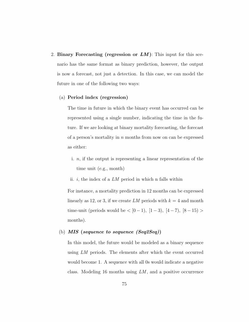
2. Binary Forecasting (regression or LM ): This input for this sce-
nario has the same format as binary prediction, however, the output
is now a forecast, not just a detection. In this case, we can model the
future in one of the following two ways:
(a) Period index (regression)
The time in future in which the binary event has occurred can be
represented using a single number, indicating the time in the fu-
ture. If we are looking at binary mortality forecasting, the forecast
of a person’s mortality in n months from now on can be expressed
as either:
i. n, if the output is representing a linear representation of the
time unit (e.g., month)
ii. i, the index of a LM period in which n falls within
For instance, a mortality prediction in 12 months can be expressed
linearly as 12, or 3, if we create LM periods with k = 4 and month
time-unit (periods would be < [0− 1), [1− 3), [4− 7), [8− 15) >
months).
(b) MIS (sequence to sequence (Seq2Seq))
In this model, the future would be modeled as a binary sequence
using LM periods. The elements after which the event occurred
would become 1. A sequence with all 0s would indicate a negative
class. Modeling 16 months using LM , and a positive occurrence
75

at month 9 would be modeled as < 0, 0, 0, 1 >. At this point, we
believe this would not give us any advantage over 2(a)ii for binary
forecasting, especially considering complexity of the model, and
the custom learning and evaluation metrics required for it (which
is not explored).
3. Multivariate Forecasting: Multivariate forecasting can be done us-
ing time-series or other techniques via LM . When the input data is
not suitable for time-series forecasting (explained in the previous chap-
ters), LM can be used. In this case, the only model would be a Seq2Seq
model with both input and output modeled using LM . For example,
diagnosis forecasting model with the shape of k × d 7→ k′ × d′.
5.5 Evaluation and Loss Metrics
Loss functions used for training neural networks are critical for proper train-
ing. Common loss functions do not account for element-wise exponential
increase in value. The proposed metrics calculates the actual errors in time
units used by LM .
LM periods add a skewness in time modeling due to exponentiation, and
thus for regression using LM periods 2(a)ii regular metrics such as mean
squared error (MSE) are not ideal. Thus, for binary forecasting using period
index (regression method) via LM periods, we introduce a new loss function
and metric called as tolerance error (TE), defined as follows:
76

Definition 5.5.1.
TE =
∣∣∣∣(2y − 2p)
2t
∣∣∣∣ (5.21)
where y=true value, p=predicted value, and t ∈ 1, 2, ..., k, is a tolerance
parameter defined for the problem.
TE calculates the exact difference between two values in terms of time unit.
For example, an error of 1 unit has a different meaning when this difference
is between 1 and 2 versus 4 and 5. The latter is 16 units of time difference
compared to only 2 units of time in difference. That is why common metrics
are not accurate for tensors mapped with LM .
The denominator determines a tolerance that is acceptable for each prob-
lem. For instance, in mortality prediction, we may or may not be interested
in whether the system is able to forecast accurate mortality withing a few
seconds or even days. This indication can be seen in the metric’s custom
design.
TE is suitable only for binary forecasting using the period index framed as
a regression problem. For sequence to sequence models using LM , a new
metric is required.
The following metric called as mean tolerance error (MTE) is suitable for
Seq2Seq analysis and is defined as follows:
Definition 5.5.2.
MTE =
√√√√ 1
n× F ×K
F∑i=1
K∑j=1
(|Yij − Pij| ∗ 2j
2t
)2
(5.22)
77

where Y and P , are true values and predicted values, respectively, and t ∈
1, 2, ..., k, is a tolerance parameter defined for the problem. F and K are
number of variables and the MIS length respectively and n is the number of
samples.
MTE can be used as a metric; however, to be used as a loss function as well,
it needs to be a differentiable function. Thus, given Y and P are tensors, we
rewrite MTE in a tensor multiplication form as follows:
MTE(Y, P ) =√∑
(|Y − P | ∗M)2 (5.23)
where M is a constant matrix defined as:
Mji =2i−t√F ×K
, for i ∈ 0, ..., K − 1 and j ∈ 0, ..., F − 1 (5.24)
MTE in tensor notation is now easily defined using differentiable functions
of the tensorflow kernel functions in order to be used as a loss function.
5.6 Applications
LM opens the door to many predictive analytics areas, healthcare in par-
ticular, by addressing the challenge of mapping long-term periods to concise
representations.
1. Healthcare
78

1 2 3 4 5 6 7 81 0 1 2 3 4 5 6 72 1 0 1 2 3 4 5 63 2 1 0 1 2 3 4 54 3 2 1 0 1 2 3 45 4 3 2 1 0 1 2 36 5 4 3 2 1 0 1 27 6 5 4 3 2 1 0 18 7 6 5 4 3 2 1 0
(a) MSE heatmap for k=8
1 2 3 4 5 6 7 81 0 0 0 1 2 4 8 162 0 0 0 1 2 4 8 163 0 0 0 1 2 4 8 164 1 1 1 0 1 3 7 155 2 2 2 1 0 2 6 146 4 4 4 3 2 0 4 127 8 8 8 7 6 4 0 88 16 16 16 15 14 12 8 0
(b) TE heatmap for k=8 and t=4
1 2 3 4 5 6 7 8 9 10 11 12 13 14 15 16 17 18 19 20 21 22 23 24 25 26 27 28 29 30 31 321 0 1 2 3 4 5 6 7 8 9 10 11 12 13 14 15 16 17 18 19 20 21 22 23 24 25 26 27 28 29 30 312 1 0 1 2 3 4 5 6 7 8 9 10 11 12 13 14 15 16 17 18 19 20 21 22 23 24 25 26 27 28 29 303 2 1 0 1 2 3 4 5 6 7 8 9 10 11 12 13 14 15 16 17 18 19 20 21 22 23 24 25 26 27 28 294 3 2 1 0 1 2 3 4 5 6 7 8 9 10 11 12 13 14 15 16 17 18 19 20 21 22 23 24 25 26 27 285 4 3 2 1 0 1 2 3 4 5 6 7 8 9 10 11 12 13 14 15 16 17 18 19 20 21 22 23 24 25 26 276 5 4 3 2 1 0 1 2 3 4 5 6 7 8 9 10 11 12 13 14 15 16 17 18 19 20 21 22 23 24 25 267 6 5 4 3 2 1 0 1 2 3 4 5 6 7 8 9 10 11 12 13 14 15 16 17 18 19 20 21 22 23 24 258 7 6 5 4 3 2 1 0 1 2 3 4 5 6 7 8 9 10 11 12 13 14 15 16 17 18 19 20 21 22 23 249 8 7 6 5 4 3 2 1 0 1 2 3 4 5 6 7 8 9 10 11 12 13 14 15 16 17 18 19 20 21 22 23
10 9 8 7 6 5 4 3 2 1 0 1 2 3 4 5 6 7 8 9 10 11 12 13 14 15 16 17 18 19 20 21 2211 10 9 8 7 6 5 4 3 2 1 0 1 2 3 4 5 6 7 8 9 10 11 12 13 14 15 16 17 18 19 20 2112 11 10 9 8 7 6 5 4 3 2 1 0 1 2 3 4 5 6 7 8 9 10 11 12 13 14 15 16 17 18 19 2013 12 11 10 9 8 7 6 5 4 3 2 1 0 1 2 3 4 5 6 7 8 9 10 11 12 13 14 15 16 17 18 1914 13 12 11 10 9 8 7 6 5 4 3 2 1 0 1 2 3 4 5 6 7 8 9 10 11 12 13 14 15 16 17 1815 14 13 12 11 10 9 8 7 6 5 4 3 2 1 0 1 2 3 4 5 6 7 8 9 10 11 12 13 14 15 16 1716 15 14 13 12 11 10 9 8 7 6 5 4 3 2 1 0 1 2 3 4 5 6 7 8 9 10 11 12 13 14 15 1617 16 15 14 13 12 11 10 9 8 7 6 5 4 3 2 1 0 1 2 3 4 5 6 7 8 9 10 11 12 13 14 1518 17 16 15 14 13 12 11 10 9 8 7 6 5 4 3 2 1 0 1 2 3 4 5 6 7 8 9 10 11 12 13 1419 18 17 16 15 14 13 12 11 10 9 8 7 6 5 4 3 2 1 0 1 2 3 4 5 6 7 8 9 10 11 12 1320 19 18 17 16 15 14 13 12 11 10 9 8 7 6 5 4 3 2 1 0 1 2 3 4 5 6 7 8 9 10 11 1221 20 19 18 17 16 15 14 13 12 11 10 9 8 7 6 5 4 3 2 1 0 1 2 3 4 5 6 7 8 9 10 1122 21 20 19 18 17 16 15 14 13 12 11 10 9 8 7 6 5 4 3 2 1 0 1 2 3 4 5 6 7 8 9 1023 22 21 20 19 18 17 16 15 14 13 12 11 10 9 8 7 6 5 4 3 2 1 0 1 2 3 4 5 6 7 8 924 23 22 21 20 19 18 17 16 15 14 13 12 11 10 9 8 7 6 5 4 3 2 1 0 1 2 3 4 5 6 7 825 24 23 22 21 20 19 18 17 16 15 14 13 12 11 10 9 8 7 6 5 4 3 2 1 0 1 2 3 4 5 6 726 25 24 23 22 21 20 19 18 17 16 15 14 13 12 11 10 9 8 7 6 5 4 3 2 1 0 1 2 3 4 5 627 26 25 24 23 22 21 20 19 18 17 16 15 14 13 12 11 10 9 8 7 6 5 4 3 2 1 0 1 2 3 4 528 27 26 25 24 23 22 21 20 19 18 17 16 15 14 13 12 11 10 9 8 7 6 5 4 3 2 1 0 1 2 3 429 28 27 26 25 24 23 22 21 20 19 18 17 16 15 14 13 12 11 10 9 8 7 6 5 4 3 2 1 0 1 2 330 29 28 27 26 25 24 23 22 21 20 19 18 17 16 15 14 13 12 11 10 9 8 7 6 5 4 3 2 1 0 1 231 30 29 28 27 26 25 24 23 22 21 20 19 18 17 16 15 14 13 12 11 10 9 8 7 6 5 4 3 2 1 0 132 31 30 29 28 27 26 25 24 23 22 21 20 19 18 17 16 15 14 13 12 11 10 9 8 7 6 5 4 3 2 1 0
Predicted (p)
Actual (y)
(c) MSE heatmap for k=8 and t=4
1 2 3 4 5 6 7 8 9 10 11 12 13 14 15 16 17 18 19 20 21 22 23 24 25 26 27 28 29 30 31 321 0 0 0 0 0 0 0 0 1 2 4 8 15 31 62 ## ## ## ## ## ## ## ## ## ## ## ## ## ## ## ## ##2 0 0 0 0 0 0 0 0 1 2 4 8 15 31 62 ## ## ## ## ## ## ## ## ## ## ## ## ## ## ## ## ##3 0 0 0 0 0 0 0 0 1 2 4 8 15 31 62 ## ## ## ## ## ## ## ## ## ## ## ## ## ## ## ## ##4 0 0 0 0 0 0 0 0 1 2 4 8 15 31 62 ## ## ## ## ## ## ## ## ## ## ## ## ## ## ## ## ##5 0 0 0 0 0 0 0 0 1 2 4 8 15 31 62 ## ## ## ## ## ## ## ## ## ## ## ## ## ## ## ## ##6 0 0 0 0 0 0 0 0 1 2 4 8 15 31 62 ## ## ## ## ## ## ## ## ## ## ## ## ## ## ## ## ##7 0 0 0 0 0 0 0 0 1 2 4 8 15 31 62 ## ## ## ## ## ## ## ## ## ## ## ## ## ## ## ## ##8 0 0 0 0 0 0 0 0 0 1 3 7 15 30 61 ## ## ## ## ## ## ## ## ## ## ## ## ## ## ## ## ##9 1 1 1 1 1 1 1 0 0 1 3 7 15 30 61 ## ## ## ## ## ## ## ## ## ## ## ## ## ## ## ## ##
10 2 2 2 2 2 2 2 1 1 0 2 6 14 29 60 ## ## ## ## ## ## ## ## ## ## ## ## ## ## ## ## ##11 4 4 4 4 4 4 4 3 3 2 0 4 12 27 58 ## ## ## ## ## ## ## ## ## ## ## ## ## ## ## ## ##12 8 8 8 8 8 8 8 7 7 6 4 0 8 23 54 ## ## ## ## ## ## ## ## ## ## ## ## ## ## ## ## ##13 15 15 15 15 15 15 15 15 15 14 12 8 0 15 46 ## ## ## ## ## ## ## ## ## ## ## ## ## ## ## ## ##14 31 31 31 31 31 31 31 30 30 29 27 23 15 0 31 93 ## ## ## ## ## ## ## ## ## ## ## ## ## ## ## ##15 62 62 62 62 62 62 62 61 61 60 58 54 46 31 0 62 ## ## ## ## ## ## ## ## ## ## ## ## ## ## ## ##16 ## ## ## ## ## ## ## ## ## ## ## ## ## 93 62 0 ## ## ## ## ## ## ## ## ## ## ## ## ## ## ## ##17 ## ## ## ## ## ## ## ## ## ## ## ## ## ## ## ## 0 ## ## ## ## ## ## ## ## ## ## ## ## ## ## ##18 ## ## ## ## ## ## ## ## ## ## ## ## ## ## ## ## ## 0 ## ## ## ## ## ## ## ## ## ## ## ## ## ##19 ## ## ## ## ## ## ## ## ## ## ## ## ## ## ## ## ## ## 0 ## ## ## ## ## ## ## ## ## ## ## ## ##20 ## ## ## ## ## ## ## ## ## ## ## ## ## ## ## ## ## ## ## 0 ## ## ## ## ## ## ## ## ## ## ## ##21 ## ## ## ## ## ## ## ## ## ## ## ## ## ## ## ## ## ## ## ## 0 ## ## ## ## ## ## ## ## ## ## ##22 ## ## ## ## ## ## ## ## ## ## ## ## ## ## ## ## ## ## ## ## ## 0 ## ## ## ## ## ## ## ## ## ##23 ## ## ## ## ## ## ## ## ## ## ## ## ## ## ## ## ## ## ## ## ## ## 0 ## ## ## ## ## ## ## ## ##24 ## ## ## ## ## ## ## ## ## ## ## ## ## ## ## ## ## ## ## ## ## ## ## 0 ## ## ## ## ## ## ## ##25 ## ## ## ## ## ## ## ## ## ## ## ## ## ## ## ## ## ## ## ## ## ## ## ## 0 ## ## ## ## ## ## ##26 ## ## ## ## ## ## ## ## ## ## ## ## ## ## ## ## ## ## ## ## ## ## ## ## ## 0 ## ## ## ## ## ##27 ## ## ## ## ## ## ## ## ## ## ## ## ## ## ## ## ## ## ## ## ## ## ## ## ## ## 0 ## ## ## ## ##28 ## ## ## ## ## ## ## ## ## ## ## ## ## ## ## ## ## ## ## ## ## ## ## ## ## ## ## 0 ## ## ## ##29 ## ## ## ## ## ## ## ## ## ## ## ## ## ## ## ## ## ## ## ## ## ## ## ## ## ## ## ## 0 ## ## ##30 ## ## ## ## ## ## ## ## ## ## ## ## ## ## ## ## ## ## ## ## ## ## ## ## ## ## ## ## ## 0 ## ##31 ## ## ## ## ## ## ## ## ## ## ## ## ## ## ## ## ## ## ## ## ## ## ## ## ## ## ## ## ## ## 0 ##32 ## ## ## ## ## ## ## ## ## ## ## ## ## ## ## ## ## ## ## ## ## ## ## ## ## ## ## ## ## ## ## 0
Predicted (p)
Actual (y)
(d) TE heatmap for k=32 and t=23 (1month)
Figure 5.6: The heatmap for MSE versus TE for k = 8 ((a), (b)) and 32((c), (d)). Both axis are index values upto k for either true value y (y-axis)or predicted value p (x-axis). The MSE cannot differentiate between thescale of difference on bigger index values while TE produces a larger error ifthe difference between predicted and true value has a different exponentialmeaning. For example, if the true value is 4 ((a), (b)), the predicted index2 is much closer to the actual value than the index 6. TE considers this,whereas MSE is unable to differentiate the two.
79

(a) Disease Diagnosis
(b) Anomaly Prediciton
(c) Cancer Care
(d) Post-surgery Monitoring
(e) Self Care
2. Lifestyle
(a) Life-style Choices
(b) Career Planning
(c) Investment Options
(d) Weight Management
(e) Parenting
3. Management
(a) Hiring Decisions
(b) Career Predictions
(c) Team Management
(d) Risk Management
(e) Project Planning
80

5.7 Summary
The proposed LM opens the door to many predictive analytics areas, health-
care in particular, by addressing the challenge of mapping long-term periods
to concise representations. For example, in healthcare, LM could be used
for disease diagnosis, anomaly prediction, cancer, post-surgery monitoring,
and in-home care. It could also be applied in lifestyle planning (e.g. career
planning, investment, fitness, weight management, and parenting) and in
management (e.g. team and risk management, project planning, and hiring
decision).
The main advantages of LM can be summarized in the following:
Enabling the modeling of history and future in a concise sequence
Decreasing the input size and the parameters of deep RNNs
Scalable (Maps long sequences)
Creating fixed-sized (or short variable sized) sequences
Missing values tolerance
Maintaining time representation
Emphasizing on recent data
Customizability
Can become a standard for temporal modeling
81

Chapter 6
Life Model Case Studies
6.1 Introduction
In this chapter, the experimental results for the following case-studies using
LM and comparison with previous study results are provided:
1. Fall Prediction and Forecasting
2. Mortality Prediction and Forecasting
3. Diagnosis and Procedures Forecasting
4. Diagnosis Prediction using simulated data
5. Activity Forecasting
82

6.2 Test Metrics
To evaluate the proposed solution, several metrics are used for different sub-
systems. Based on the case studies, predictive performance with focus on
comparison with the recent techniques (if possible) is considered.
Common metrics in machine learning literature to be used are as follows
1. Classification Metrics
Most machine learning algorithm and data structure techniques are
evaluated and compared by the set of precision and recall definitions
based on true positives (TP), true negatives (TN), false positives (FP),
and false negatives (FN). These metrics may have different names and
labels in different domains. In medicine for example, Type I and Type
II errors stand for FP and FN , respectively.
The two most commonly used metrics to compare binary prediction
models are AuROC and Brier score. Brier score is a score function
that measures the accuracy of probabilistic predictions. The lower the
Brier score, the more accurate and calibrated the predictions are. In
the common form, it is the mean squared error of the prediction.
These are used to compare LM algorithms and LSTM -based experi-
mental results with other techniques. Calibration and receiver operat-
ing characteristic (ROC) plots is also provided for such models.
2. Big O analysis and Responsiveness
83

Algorithm complexities are already provided for key algorithms in the
proposed solution. To test the deep learning convergence and mapping
processing speeds, we conduct empirical tests. Speed is the measure of
how fast each component of the system can finish their specific task.
3. Regression and Forecasting
For forecasting using the proposed methods described earlier in sec-
tion 5.4, in addition to regular regression metrics like MSE , proposed
metrics for LM which are TE and MTE are also used.
6.3 Test Datasets
Finding suitable medical and health data for research is always challenging.
There are three reasons for this difficulty:
1. Privacy issues.
2. Finding patients with desired diseases.
3. Long-term and robust monitoring for all subjects in the study.
Although electronic medical health records are now available for many of
the patients, these data sets are highly confidential, and do not contain real-
time health data. Thus, for novel techniques and approaches, most of the
proposed methods use either simulated data [14, 34], or datasets that are
not usually accessible by other researchers [34, 8, 7, 67]. Some datasets are
84

available that are too specific, e.g., for a specific group of diseases (patients
with diabetes only [68]). For example, the Tim Van Kastern’s public datasets
[69] provides activity recognition data of three homes. However, the data is
about activities only, and does not contain any health sensory data.
In this research, we used the following sources of data:
1. MIMIC III: MIMIC III [11, 70] is a large, freely-available database
comprising de-identified health-related data associated with over 45,000
patients who stayed in critical care units of the Beth Israel Deaconess
Medical Center between 2001 and 2012. The database includes in-
formation such as demographics, vital sign measurements made at
the bedside, laboratory test results, procedures, medications, caregiver
notes, imaging reports, and mortality (both in and out of hospital).
It specifically contains 68k ICD9 diagnosis codes, 80k lab codes, 116k
medication codes (from RxNorm), and the data contains variable length
records with missing values. The database is around 80GB in size with-
out the waveform data. MIMIC supports a diverse range of analytic
studies spanning epidemiology, clinical decision-rule improvement, and
electronic tool development. It is notable for three factors:
It is freely available to researchers worldwide
It encompasses a diverse and very large population of ICD patients
It contains high temporal resolution data including lab results,
electronic documentation, and bedside monitor trends and wave-
85

forms.
2. University of Rzeszow fall dataset (URFD): The proposed LM
model has also been tested and verified on a dataset called URFD
[71, 72]. The dataset contains 70 cases (30 falls and 40 normal daily
activities). We used the raw accelerometer data provided which in-
cludes 3D acceleration vector of ax(t), ay(t), and az(t) with time stamp
in milliseconds. The norm of the acceleration vector (magnitude) was
also provided. The data had been recorded in 30 Hz and each sample
is around 5-16 seconds.
3. Tim Van Kastern’s: Tim Van Kastern’s public datasets [69] for one
home for 28 days is used for activity forecasting. Each activity had a
start and end date.
4. Simulated Data
For preliminary testing and comparing algorithms, a temporal health
data simulator is implemented which is able to generate temporal ab-
stractions for any number of patients, temporal variables, and diagno-
sis/anomaly classes. The simulator starts with creating a normal pa-
tient and then injects disease patterns for a specific class by a specific
ratio. For example, for a patient with high blood pressure, the simu-
lator can replace 15% of blood pressure abstraction values to “High”
and 5% to “Very High”. Often each patient may have more than one
disease. For instance, a patient may have high blood pressure and high
86

last admissionprevious admissions
time
(training data) (forecasting target)
cut-off point for time shift
Figure 6.1: The forecasting data in MIMIC III dataset is prepared by shiftingthe final admission of each patient into future and forecasting based on theprevious admissions.
glucose symptoms simultaneously. Then each patient will be labeled
with one or more than one diagnosis for testing.
6.4 Mortality Models
To forecast mortality in the future, from over 34,000 valid cases in MIMIC
III dataset, only a little over 5200 patients had two or more admissions. Here,
both a mortality forecasting model is created on this subset and a mortality
prediction/detection model is trained on all valid records.
6.4.1 Mortality Forecasting
LM mapping enables forecasting for temporal sequences. The future is mod-
eled using LM mappings and the index of the binary target in the mapping
87
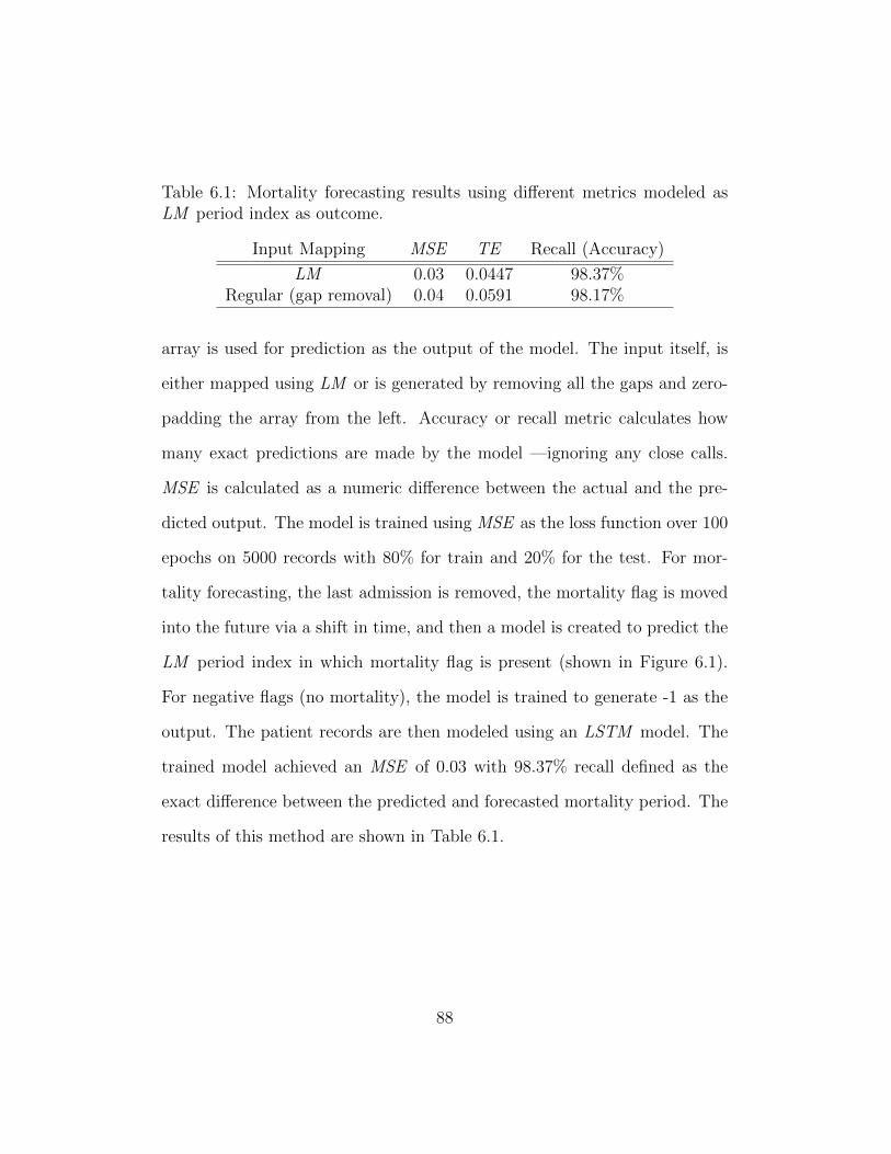
Table 6.1: Mortality forecasting results using different metrics modeled asLM period index as outcome.
Input Mapping MSE TE Recall (Accuracy)
LM 0.03 0.0447 98.37%Regular (gap removal) 0.04 0.0591 98.17%
array is used for prediction as the output of the model. The input itself, is
either mapped using LM or is generated by removing all the gaps and zero-
padding the array from the left. Accuracy or recall metric calculates how
many exact predictions are made by the model —ignoring any close calls.
MSE is calculated as a numeric difference between the actual and the pre-
dicted output. The model is trained using MSE as the loss function over 100
epochs on 5000 records with 80% for train and 20% for the test. For mor-
tality forecasting, the last admission is removed, the mortality flag is moved
into the future via a shift in time, and then a model is created to predict the
LM period index in which mortality flag is present (shown in Figure 6.1).
For negative flags (no mortality), the model is trained to generate -1 as the
output. The patient records are then modeled using an LSTM model. The
trained model achieved an MSE of 0.03 with 98.37% recall defined as the
exact difference between the predicted and forecasted mortality period. The
results of this method are shown in Table 6.1.
88

6.4.2 Mortality Detection
To evaluate the proposed LM for prediction, MIMIC III dataset is used to
predict patient mortality given the admission data. The goal is to predict
whether a patient has expired followed by their admissions as a sequence
binary classification.
Data From the total patients in MIMIC III hospital, those patients aged
15 and up, who are not organ donors, and have chart data are selected. The
result is a total of 34,755 patients. From these patients, 369 had invalid
discharge and death date which could not be used for this experiment. From
the remaining 34,419 patients, we used the first 1000, 10,000, and 34,000
subset of patient records to test the proposed method. For each patient,
a list of admissions, and for each admission, the assigned ICD9 diagnosis
codes and procedure codes were extracted. The patients had a total of 6,400
distinct assigned diagnosis codes and 1,971 distinct procedure codes, for a
total of 8,371 possible flags per admission per patient. Because the number
of diagnoses per patient per visit is 10, an example of the data for a patient
looks like the following list:
1, 1, 1, 1, 0, 0, 0, 1, 0, 1, 0, 0, 0, ..., 0s, ..., 1, 0, 0, 1, 0, 1, ...0s
This list indicates a hospital visit in which ones (1s) in the list indicate the
presence of a specific diagnosis in that admission, followed by many zeros
89

which indicate the absence of other admissions and ending with ones and
zeros indicating the procedures that were performed on the patient. Each
record is accompanied by a date, which is used by LM to assign it to the
correct element.
LM is used to create a single fixed-size tensor for each patient, regardless
of number of admissions. An optimized implementation of LM written in
C# is used to map each patient data to a normalized MIS of length 32.
Each MIS element consists of a one-hot-code embedding of all ICD9 codes
(8,371 codes). To compare the effectiveness of LM mapping, a baseline MIS
which uses fixed-sized intervals is also generated. The periods in LM tensor
is mapped using the LM algorithm, and the periods in the fixed-size intervals
have the size 1k∆T = 1
32∆T .
Model The learning model used is the same LSTM network, with input
size of 8, 371× 32, followed by a recurrent dropout layer of 0.2, and another
dropout layer of 0.2, with a final 32× 1 dense layer as the output layer with
sigmoid activation. The dropout layers help prevent overfitting by ignoring a
random subset of weights during training. The model is trained using Adam
optimizer with binary crossentropy as the loss function to enable binary
output. For testing, Keras 2.0 wrapper on top of Tensorflow 1.4 toolkit is
used. Tensorflow is a popular open-source library for dataflow programming
mostly used for deep learning training. Models are trained on an Azure NC24
virtual machine with 4 Nvidia Tesla K80 GPUs , 24 Intel Xeon cores. This
90
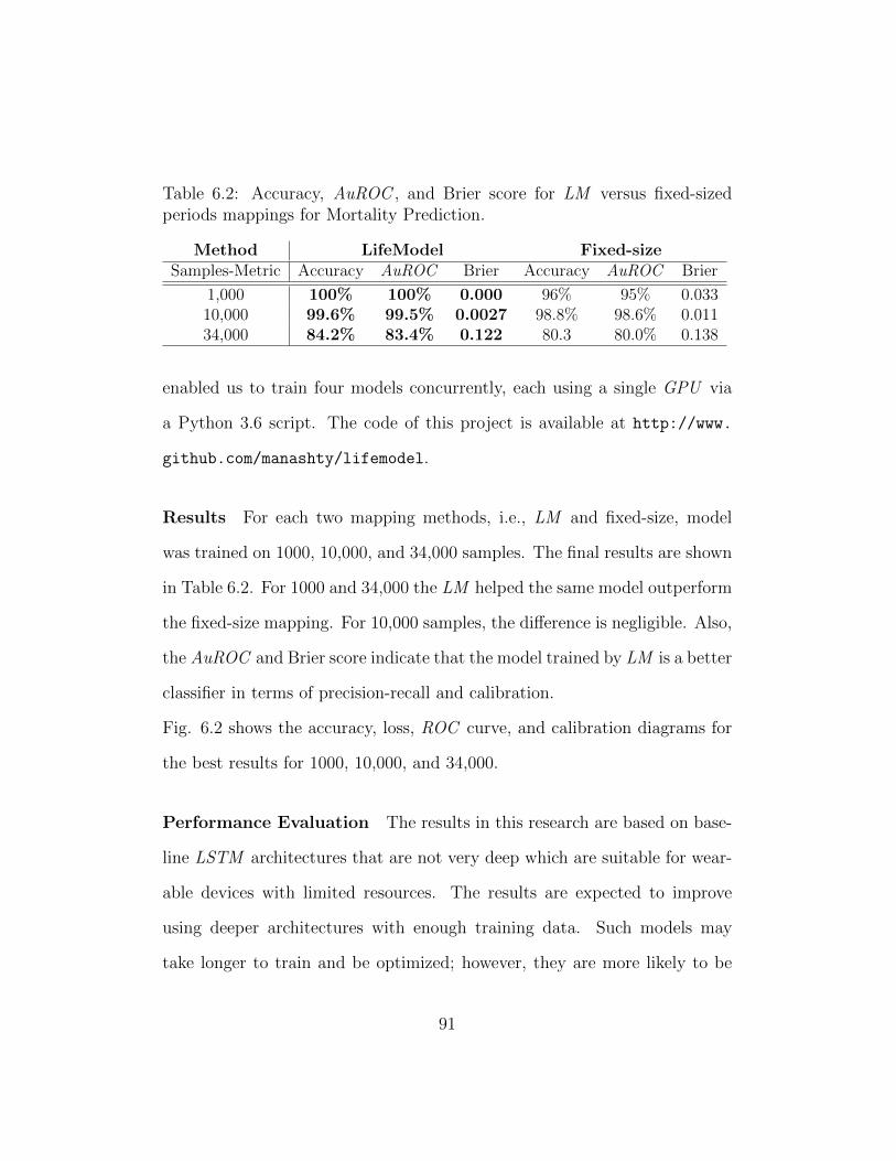
Table 6.2: Accuracy, AuROC , and Brier score for LM versus fixed-sizedperiods mappings for Mortality Prediction.
Method LifeModel Fixed-sizeSamples-Metric Accuracy AuROC Brier Accuracy AuROC Brier
1,000 100% 100% 0.000 96% 95% 0.03310,000 99.6% 99.5% 0.0027 98.8% 98.6% 0.01134,000 84.2% 83.4% 0.122 80.3 80.0% 0.138
enabled us to train four models concurrently, each using a single GPU via
a Python 3.6 script. The code of this project is available at http://www.
github.com/manashty/lifemodel.
Results For each two mapping methods, i.e., LM and fixed-size, model
was trained on 1000, 10,000, and 34,000 samples. The final results are shown
in Table 6.2. For 1000 and 34,000 the LM helped the same model outperform
the fixed-size mapping. For 10,000 samples, the difference is negligible. Also,
the AuROC and Brier score indicate that the model trained by LM is a better
classifier in terms of precision-recall and calibration.
Fig. 6.2 shows the accuracy, loss, ROC curve, and calibration diagrams for
the best results for 1000, 10,000, and 34,000.
Performance Evaluation The results in this research are based on base-
line LSTM architectures that are not very deep which are suitable for wear-
able devices with limited resources. The results are expected to improve
using deeper architectures with enough training data. Such models may
take longer to train and be optimized; however, they are more likely to be
91

0 1 2 3 4 5epoch
0.76
0.78
0.80
0.82
0.84
0.86
0.88
acc
ura
cy
model accuracy
train LM 34k
test LM 34k
train FS 34k
test FS 34k
0 5 10 15 20 25 30epoch
0.75
0.80
0.85
0.90
0.95
1.00
acc
ura
cy
model accuracy
train LM 10k
test LM 10k
train FS 10k
test FS 10k
0 1 2 3 4 5 6 7 8 9epoch
0.65
0.70
0.75
0.80
0.85
0.90
0.95
1.00
acc
ura
cy
model accuracy
train LM 1k
test LM 1k
train FS 1k
test FS 1k
0 1 2 3 4 5epoch
0.25
0.30
0.35
0.40
0.45
0.50
0.55
loss
model loss
train LM 34k
test LM 34k
train FS 34k
test FS 34k
0 5 10 15 20 25 30epoch
0.0
0.1
0.2
0.3
0.4
0.5
0.6
loss
model loss
train LM 10k
test LM 10k
train FS 10k
test FS 10k
0 1 2 3 4 5 6 7 8 9epoch
0.0
0.1
0.2
0.3
0.4
0.5
0.6
0.7
loss
model loss
train LM 1k
test LM 1k
train FS 1k
test FS 1k
0.0 0.2 0.4 0.6 0.8 1.0False Positive Rate
0.0
0.2
0.4
0.6
0.8
1.0
Tru
e P
osi
tive R
ate
Receiver operating characteristic
ROC curve LM 34k (area = 0.83)
ROC curve FS 34k (area = 0.80)
0.0 0.2 0.4 0.6 0.8 1.0False Positive Rate
0.0
0.2
0.4
0.6
0.8
1.0
Tru
e P
osi
tive R
ate
Receiver operating characteristic
ROC curve LM 10k (area = 1.00)
ROC curve FS 10k (area = 0.99)
0.0 0.2 0.4 0.6 0.8 1.0False Positive Rate
0.0
0.2
0.4
0.6
0.8
1.0
Tru
e P
osi
tive R
ate
Receiver operating characteristic
ROC curve LM 1k (area = 1.00)
ROC curve FS 1k (area = 0.95)
0.0 0.2 0.4 0.6 0.8 1.0Mean predicted value
0.0
0.2
0.4
0.6
0.8
1.0
Fract
ion o
f posi
tives
Calibration plots (reliability curve)
Perfectly calibrated
LM 34k (0.122)
FS 34k (0.138)
0.0 0.2 0.4 0.6 0.8 1.0Mean predicted value
0
100
200
300
400
500
600
Count
LM 34k FS 34k
(a)
0.0 0.2 0.4 0.6 0.8 1.0Mean predicted value
0.0
0.2
0.4
0.6
0.8
1.0
Fract
ion o
f posi
tives
Calibration plots (reliability curve)
Perfectly calibrated
LM 10k (0.003)
FS 10k (0.011)
0.0 0.2 0.4 0.6 0.8 1.0Mean predicted value
0
50
100
150
200
250
300
Count
LM 10k FS 10k
(b)
0.0 0.2 0.4 0.6 0.8 1.0Mean predicted value
0.0
0.2
0.4
0.6
0.8
1.0
Fract
ion o
f posi
tives
Calibration plots (reliability curve)
Perfectly calibrated
LM 1k (0.001)
FS 1k (0.033)
0.0 0.2 0.4 0.6 0.8 1.0Mean predicted value
0
5
10
15
20
25
30
Count
LM 1k FS 1k
(c)
Figure 6.2: Training and testing plots for mortality prediction on MIMICIII dataset for (a) 34,000 (34k), (b) 10,000 (10k), and (c) 1000(1k)patients. For each sample size, accuracy, loss, ROC curve (and AuROC(the higher the better)), and the model calibration with the brier score foreach method (the lower the better) is displayed. Results are for using LMmapping with n=5, and k=32 versus 32-element fixed-size (FS) MIS .
92

suitable for client-server environments. The proposed system architecture is
aiming to be considered real-time, because although the training takes hours
and days to complete, once completed, they can be used to evaluate records
within milliseconds, as the weights are transferred to the chips. The LM
mapping time is also real-time, with more than 30 samples per second in a
single thread for this large data-set. The implementation is using dictionary
hash maps which has O(1) complexity and can be transferred to hardware.
6.4.3 Diagnosis and Procedures Forecasting
Diagnosis forecasting is defined as predicting the exact diagnosis and pro-
cedures codes in the future defined by LM . To forecast MTS in the future,
by shifting the final admission of each patient to the future and placing the
second last admission to time zero, a sequence to sequence problem is mod-
eled using LM . With more than 250,000 (32 × 8731) input variables and the
same number of output variables, it may be ambitious to train a model with
only 5000 samples. However, to find the effectiveness of the proposed MTE
metric, this metric is compared with MSE for training effectiveness.
The proposed MTE metric is used both as the loss function and the metric
to evaluate the model, comparing it with MSE performance as loss function.
MSE and MTE are metrics that are calculated as a numeric difference be-
tween the actual and the predicted output. This model is again trained using
both MSE and MTE as the loss function over 100 epochs on 5000 records
(with 80%/20% train/test ratio).
93

Training the LSTM model using the proposed MTE function results in lower
MTE , which is a more meaningful metric for LM . The t-test statistics of the
differences of the means indicates that there is a significant difference between
the two results (MTE is significantly lower (p-value< 2.2e−16)) (Figure 6.3).
6.4.4 Discussion
From the loss and accuracy plots in Figure 6.2 for 10k and 34k samples,
it can be observed that the LM converges faster than fixed-sized mapping
although the fixed-size mapping eventually converges to the same point. This
is a critical factor for real-time and large-scale problems. For example, each
epoch of training for 34,000 patients takes about 2.5 hours using a modern
GPU in the virtual machine (VM) used. When redeploying a model, or
large-scale IoT data and million users are considered, a model that converges
faster has an edge on similar models with late convergence. This is shown
specially when the number of patients increase. LM can clearly capture the
temporal relation in different time-points faster than the fixed-size. This may
be due to the fact that recent data is repeated multiple times as the recency
is incorporated into LM .
94

Mean Tolerance Error (MTE) Mean Squared Error (MSE)
1.0e
−07
1.5e
−07
2.0e
−07
2.5e
−07
Loss Function
Mea
n To
lera
nce
Err
or (
MT
E)
(a)
1e−07
2e−07
3e−07
4e−07
0 100 200 300 400Epochs
Mea
n To
lera
nce
Err
or
Loss Function
MSE
MTE
(b)
Figure 6.3: (a) The boxplot for MTE of the training and testing error (mean)of a sequence to sequence model trained by either MTE or MSE over 100epochs. (b) shows the training MTE for different epochs.
95

6.5 Human Fall Prediction and Forecasting
6.5.1 Introduction
Recognizing internal activities of the human body based on biologically gen-
erated time series data is at the core of technologies used in wearable re-
habilitation devices [73] and health support systems [74]. Some commercial
examples include fitness trackers and fall detection devices. Wearable ac-
tivity recognition systems are composed of sensors, such as accelerometers,
gyroscopes or magnetic field/chemical sensors [75] and a processor used to
analyze the generated signals. Real–time and accurate interpretation of the
recorded physiological data from these devices can be considerably helpful in
the prevention and treatment of a number of diseases [76]. For instance, pa-
tients with diabetes, obesity or heart disease are often required to be closely
monitored and follow a specific exercise set as part of their treatments [77].
Similarly, patients with mental pathologies such as epilepsy can be monitored
to detect abnormal activities and therefore prevent negative consequences
[78].
However, most current commercial products only offer relatively simple met-
rics, such as step count or heartbeat and lack the complexity and computing
power for many time series forecasting problems of interest in real time. The
emergence of deep learning methodologies capable of learning multiple lay-
ers of feature hierarchies and temporal dependencies in time series problems
and increased processing capabilities in wearable technologies lay the ground
96

to perform more detailed data analysis on–node and in real time [79]. The
ability of performing more complex analysis, such as human activity classifi-
cation on the wearable device could potentially filter data streaming from the
device to host and save data bandwidth link. This data saving is more visible
in the cases where the classification task should be continuously preformed
on the patient such as in seizure detection for epileptic patients. However,
due to the high computational power and memory bandwidth required by
deep learning algorithms, full realization of such systems on wearable and
embedded medical devices is still challenging.
6.5.2 Hardware Considerations
Along with the useful aspects of the proposed model in improving the ac-
curacy of an RNN network, the reduction provided by the MIS input could
also be beneficial to hardware realizations. There are some variations on the
LSTM architecture. Consider the following model [80]:
hfn+1 = σ(W Tf · xn + bf )
hin+1 = σ(W Ti · xn + bi)
hon+1 = σ(W To · xn + bo)
hcn+1 = tanh(W Tc · xn + bc)
cn+1 = hfn cn + hcn hin;
hn+1 = hon tanh(cn);
97

where xn = [hn,un] and un, hn and cn are the input, output and cell state
vectors respectively at discrete time index, n. The operator denotes the
Hadamard element by element product. The variables hfn, hin, hon represent
the forgetting, input and output gating vectors. Finally, Wf , Wi, Wo, Wc
and bf , bi, bo, bc are the weights and biases for the different layers, respec-
tively. In this structure, the number of weights embedded in the layers is
defined as follows:
4× (HN + IWS)×HN (6.1)
where HN is the number of hidden neurons and IWS is the input window
size. Therefore, a reduction factor of X due to the MIS block could poten-
tially reduce 4×X ×HN number of weights and improve the performance
of the hardware in three directions:
Memory Consumption: Considering N bits for storing weights in
the memory, the MIS block can reduce the amount of memory stor-
age used in the hardware by a factor of 4 × X × HN × N bits. As
one of the main bottlenecks for the hardware realization of RNNs and
convolutional neural networks (CNNs) is the bandwidth required to
fetch weights in each operation, this significant reduction could be also
effective in this way.
Power Consumption: By reducing the number of weights by a factor
of 4×X×HN , the number of calculations required to produce an out-
put is also reduced. This reduction saves power consumption almost by
98
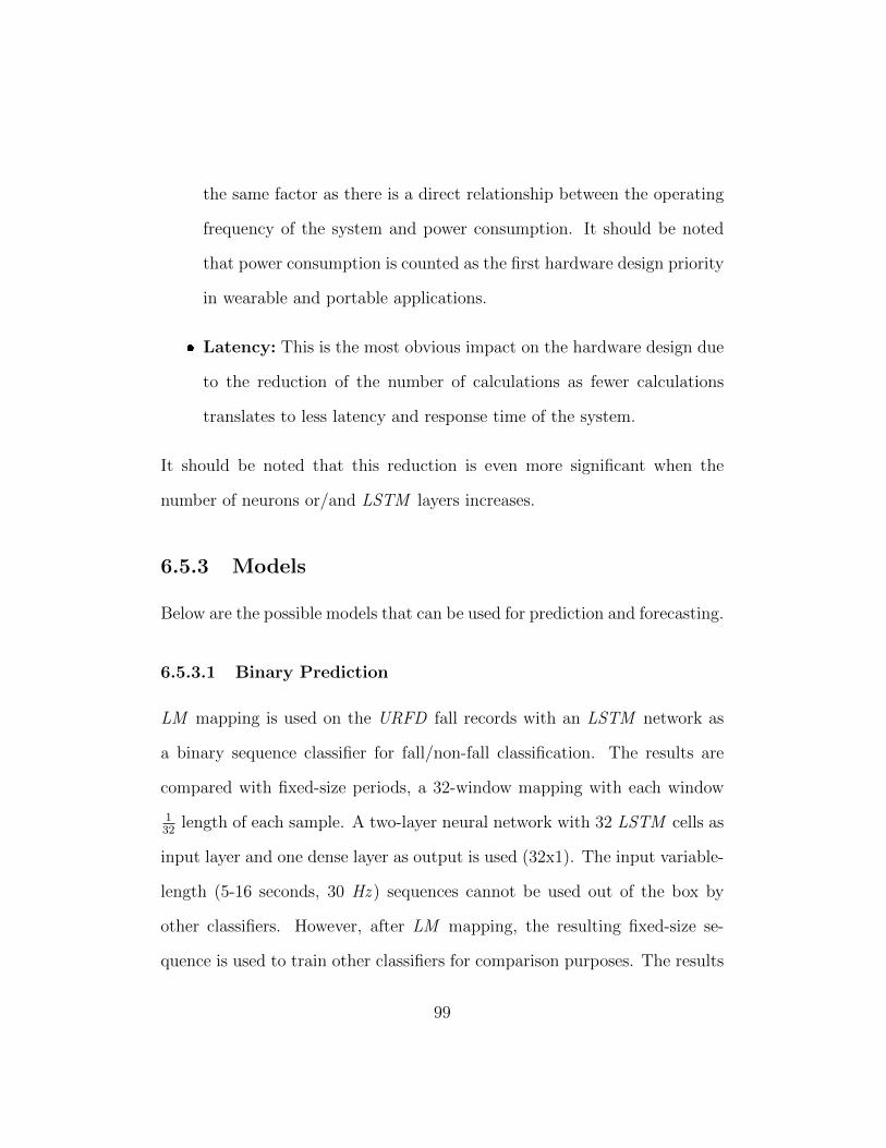
the same factor as there is a direct relationship between the operating
frequency of the system and power consumption. It should be noted
that power consumption is counted as the first hardware design priority
in wearable and portable applications.
Latency: This is the most obvious impact on the hardware design due
to the reduction of the number of calculations as fewer calculations
translates to less latency and response time of the system.
It should be noted that this reduction is even more significant when the
number of neurons or/and LSTM layers increases.
6.5.3 Models
Below are the possible models that can be used for prediction and forecasting.
6.5.3.1 Binary Prediction
LM mapping is used on the URFD fall records with an LSTM network as
a binary sequence classifier for fall/non-fall classification. The results are
compared with fixed-size periods, a 32-window mapping with each window
132
length of each sample. A two-layer neural network with 32 LSTM cells as
input layer and one dense layer as output is used (32x1). The input variable-
length (5-16 seconds, 30 Hz ) sequences cannot be used out of the box by
other classifiers. However, after LM mapping, the resulting fixed-size se-
quence is used to train other classifiers for comparison purposes. The results
99
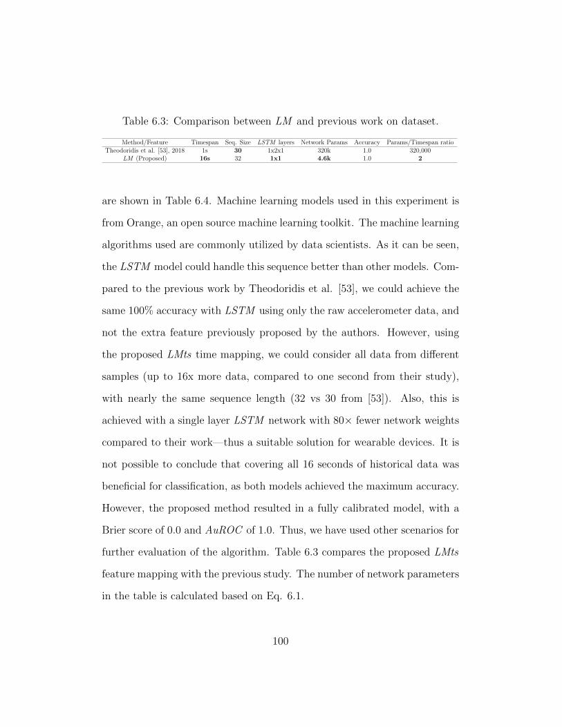
Table 6.3: Comparison between LM and previous work on dataset.
Method/Feature Timespan Seq. Size LSTM layers Network Params Accuracy Params/Timespan ratioTheodoridis et al. [53], 2018 1s 30 1x2x1 320k 1.0 320,000
LM (Proposed) 16s 32 1x1 4.6k 1.0 2
are shown in Table 6.4. Machine learning models used in this experiment is
from Orange, an open source machine learning toolkit. The machine learning
algorithms used are commonly utilized by data scientists. As it can be seen,
the LSTM model could handle this sequence better than other models. Com-
pared to the previous work by Theodoridis et al. [53], we could achieve the
same 100% accuracy with LSTM using only the raw accelerometer data, and
not the extra feature previously proposed by the authors. However, using
the proposed LMts time mapping, we could consider all data from different
samples (up to 16x more data, compared to one second from their study),
with nearly the same sequence length (32 vs 30 from [53]). Also, this is
achieved with a single layer LSTM network with 80× fewer network weights
compared to their work—thus a suitable solution for wearable devices. It is
not possible to conclude that covering all 16 seconds of historical data was
beneficial for classification, as both models achieved the maximum accuracy.
However, the proposed method resulted in a fully calibrated model, with a
Brier score of 0.0 and AuROC of 1.0. Thus, we have used other scenarios for
further evaluation of the algorithm. Table 6.3 compares the proposed LMts
feature mapping with the previous study. The number of network parameters
in the table is calculated based on Eq. 6.1.
100

Table 6.4: Performance of the LM and fixed size periods for fall prediction
Design Classifier Accuracy Precision Recall AuROC
Naiive bayes (NB) 0.843 0.939 0.775 0.904LR* 0.900 0.923 0.900 0.958
Fixed Size SVM 0.843 0.872 0.850 0.958Random forests (RF) 0.857 0.895 0.850 0.921CN2 algorithm (CN2) 0.729 0.769 0.750 0.838LSTM 0.981 0.981 0.980 0.980
NB 0.886 0.900 0.900 0.967LR 0.871 0.878 0.900 0.958
LM SVM* 0.914 0.905 0.950 0.958RF 0.871 0.860 0.925 0.954CN2 0.843 0.809 0.950 0.879LSTM 1.00 1.00 1.00 1.00
6.5.4 Fall Forecasting
To forecast falls in the future, a new dataset is created based on the URFD
fall dataset. This dataset is created by shifting the temporal data to the
right, one second at a time, to generate a new test case in which the fall
moment occurs in the future, with all the future data being discarded except
the fall time stamp. Using this method, for all fall records ranging from 2-15
seconds, a little over 500 test cases are generated. The fall time stamp is then
modeled using LMts and the period index in which the fall has occurred is
given as the target of the prediction model. The history is modeled using
LMts . If no fall has occurred, the model output should be -1. Table 6.5
shows the results for the trained model using an LSTM network. As it can
be seen, using the model trained with LMts using TE as the loss function,
achieves a higher accuracy, despite missing values.
101

Table 6.5: Fall forecast results for up to 14 seconds with various metrics andlevels of missing values.
Input mapping MetricFall Forecast
all dataFall Forecast
10% missing dataFall Forecast
50% missing data
LMMSERecallTE
0.4586.96%0.01360
0.2083.15%0.01673
0.2785.56%0.02780
Fixed IntervalsMSERecallTE
0.5985.87%0.01143
0.1380.22%0.01114
0.2881.11%0.02346
6.5.5 Fall Forecasting with Missing Values
In order to evaluate the robustness of LMts with the presence of missing
values, two additional datasets with 10% and 50% of the data randomly
removed is also considered for testing and comparison. The results are in
Table 6.5. The results indicate that despite having missing values, LMts was
able to successfully forecast the fall up to 14 seconds before the fall.
6.6 Comparison with Recent Temporal Pat-
terns (RTPs)
To compare the effectiveness of the proposed ITS compared to RTP , an
experiment1 is conducted with 10,000 and 100,000 simulated patient records
using several machine learning algorithms.
1This study was presented in IDEAS 2017, UK and published in association for com-puting machinery (ACM) proceedings
102

6.6.1 Simulated Data
To generate the data, the data simulator initially generates a temporal record
of a patient p ∈ P with m different random time points and values where P
is the set of patients and m is a simulator hyper-parameter with the default
value of 100. Then segments of similar timepoints are merged together using
a sliding window to create intervals of the form (s, e)i | 0 ≤ s, e ≤ N for
temporal variables F and all random abstraction values Vf .
Defining the multivariate temporal abstraction sequence (MTAS) vector for
patient p in the form of:
~MTASp = 〈(f1, v1, s1, e1), (f2, v2, s2, e2), , (fn, vn, sn, en)〉 (6.2)
where n ≤ N, fn ∈ F is a temporal variable and F is the collection of all
temporal variables in simulation (|F | = 10 by default), and
vn ∈ V | V = “V ery Low”, “Low”, “Normal”, “High”, “V ery High”
(6.3)
is an abstract value, helps us define the initial state of each patient p in form
of a ~MTASp with vi = rand(i) | i ∈ [1, n].
After creating the random patients, each patient record (PR) is mapped to a
diagnosis d. This mapping can be showed as the following and is defined as
103

the PR:
PRp : (MTASp → dp) (6.4)
where di ∈ D is one of the |D| different diagnosis in simulation (|D| is 10
by default). The pattern injector (PI) is responsible for changing temporal
abstractions for each PR. Each di has two diagnosis signature: Primary (d1i )
and secondary (d2i ). Each diagnosis signature is a temporal pattern in form of
(F, V ). For example, (“Blood Pressure”, “V ery High”) is a diagnosis sig-
nature. The simulator randomly assigns two temporal patterns to each diag-
nosis di. Then using two global variables called pattern injection rate (PIR)
and shown as PIRj, j ∈ 1, 2 defined randomly between [0, 1) (by default
0.15 and 0.05 respectively), the PI replaces the temporal pattern (F, V ) part
of 100 ∗PIRj ∗ |MTASp| temporal abstractions to djp where j ∈ 1, 2. This
replacement changes up to 20% of the patient records based on the patient-
specific diagnosis.
6.6.2 Prediction Model
Presenting each PR as a sequence, makes it necessary to choose a suitable
classification algorithm. Thus, we use the LSTM cells using Microsoft cog-
nitive toolkit (CNTK) [81] to benchmark the proposed feature extractions.
As it is expected to have a sparse input data (i.e., with a lot of zeros), rec-
tifier units are used in both regular feedforward and RNN cells [82]. Next,
104

the classification results for classifying temporal sequence for diagnosis dp is
presented.
6.6.3 Results and Comparison
Simulated data is generated for |F | = 10, |V | = 5, |P | = 10, 000, 100, 000,
and K=400. RTP method is implemented based on [8] with a gap value of
5% of the time interval length N which is 500 units of time. Also, patterns up
to order 4 are collected (4-patterns). The results of the classification average
recalls are shown in Table 6.6. The first three algorithms are used from H2O
[83] machine learning package. RF is used with default 50 trees; gradient
boosting machine (GBM) is used with 50 trees as well and deep feed-forward
neural network (DFF) with rectifier activations with two hidden layers of
size 200 (200x200) is used. GBM and RF models are the most popular and
top performing machine learning models due to their boosting algorithms to
create strong models based on weak learners. For LSTM , CNTK 2.0rt is
used with the LSTM cells of size 200, dropout layer and a fully connected
layer (200) with softmax activation function for class outputs. For RTP , as
the patterns cannot be reshaped as sequential inputs, LSTM could not be
used. For others, the ITS features are presented as a flat feature list.
105

Table 6.6: Accuracy (Average Recall) results for 10,000 patients using dif-ferent techniques.
RF GBM DFF LSTM
RTP Train 76.04% 92.02% 99.99% N/ATest 69.85% 85.65% 74.25% N/A
Time (s) 67.0 184.6 47.3 N/AITS Train 77.92% 99.78% 99.99% 99.99%
Test 80.51% 88.60% 79.13% 89.4%Time (s) 100.4 214.2 56.4 80.1
Table 6.7: Accuracy (Average Recall) results for 100,000 patients using dif-ferent techniques.
RF GBM DFF LSTM
RTP Train 71.14% 76.16% 92.76% N/ATest 65.22% 54.35% 58.19% N/A
Time (s) 514 819 316 N/AITS Train 68.52% 82.24% 90.79% 95.14%
Test 69.09% 69.56% 65.07% 78.81%Time (s) 737.3 1628.2 648 1208.1
106

6.6.4 Discussion
RTP model is trained faster than ITS because it considers only the last 5% of
the time frame. However, the preparation time was twice as long compared
to ITS . Also, it seems like it is unable to capture some of the long-term
dependencies in the data. Generally, ITS is slightly better at classification
as it considers the long-term relationships. When using deep learning on
10,000 instances of data, the deep learning and GBM seems to overfit very
easily. Although the recognition rate is almost 100% in training, it can only
perform with around 80% of accuracy in testing which is slightly less than
random forests. GBM and LSTM have the same problem, although they
have the highest test average recall.
To see if larger amount of data can help with the overfitting problem, same
tests are performed using 100,000 instances. Results are shown in Table 6.7.
As it can be seen, this does not seem to solve the overfitting problem for
GBM and DFF . However, the LSTM network performs slightly better with
the sequence data given as ITS . After reviewing the confusion matrix of
the LSTM model training model, it was observed that the model is trained
efficiently by the train data. However, model does not perform well on the
test data. This is due to the overfitting problem in deep learning techniques
despite using drop-out algorithm for overcoming over-fitting. Although DFF
is prone to overfitting, the deep LSTM model seems to have been trained
more efficiently than all other models. The drop in the test results are more
tolerable than the DFF . Also, it performs better than all other algorithms
107

when trained with ITS features.
The system used for testing the algorithms is a Windows 10 Education on
a Dell OptiPlex 9020 PC with 16GB of Ram, Intel Core i7-4790 CPU @3.6
GHz with 4 cores and 8 hardware threads, and a Samsung 850 Evo 500 GB
solid state disk. H2O 3.10.4 is used for RF , GBM , and DFF and CNTK
2.0rc via Python 3.5.2 interface is used for the RNN with LSTM cells. The
running time for different models were comparable, however, RF was faster
than the other models.
6.7 Human Activity Forecasting
6.7.1 Forecasting Model
To test the LM for forecasting, Tim et. al [66] activity recognition database
is used. However, instead of activity recognition using raw sensors, the 28-
day list of activities of an individual is used to train a model to predict
the future activities based on the past activities. We generated 258 total
records from 28 days of data by sliding the pivot point of the temporal data
to create different past and future activity lists. The data was tested using
LM mapping versus a fixed-size (32) sequence represented by MIS and used
an encoder-decoder LSTM to predict a sequence of activities in the future.
The network has a dense hidden layer of size 256, with two LSTM encoder
and decoder layers of size 32 as input and output of the network. The system
was tested on the same environments as above.
108

Table 6.8: Accuracy and loss for LM versus fixed-size periods mappings foractivity recognition.
Periods Sequence Size Train Accuracy Loss Accuracy
Fixed 32 99.5 0.01 92.5LM 32 80 0.1 90.2
6.7.2 Results
The results are in table 6.8. As it can be seen, the model trained with LM
had difficulties converging however; both models achieved similar results in
test, compared to training with the same number of epochs.
6.7.3 Discussion
It appears that the network has some difficulties with LM input, due to
the fact that the activity input is in fact seasonal. The activities are being
repeated daily, and LM simply ignores it. This phenomenon is common in
time-series analysis. In fact, most time-series forecasting techniques (such as
ARIMA) first remove the following two from the data:
1. Seasonality
2. Trend
Then forecasting is performed and in the final stage, the removed seasonality
and linear trend is added back to the model. The removal and addition of
seasonality is not trivial in this case as our case is a multi-variate temporal
data with missing values and a linear trend or seasonality may be difficult
109
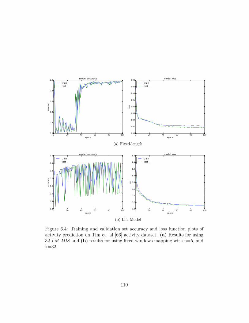
0 20 40 60 80 100epoch
0.0
0.2
0.4
0.6
0.8
1.0
acc
ura
cy
model accuracy
traintest
0 20 40 60 80 100epoch
0.00
0.01
0.02
0.03
0.04
0.05
0.06
0.07
0.08
loss
model loss
traintest
(a) Fixed-length
0 20 40 60 80 100epoch
0.3
0.4
0.5
0.6
0.7
0.8
0.9
1.0
acc
ura
cy
model accuracy
traintest
0 20 40 60 80 100epoch
0.0
0.2
0.4
0.6
0.8
1.0
1.2
1.4
1.6
loss
model loss
traintest
(b) Life Model
Figure 6.4: Training and validation set accuracy and loss function plots ofactivity prediction on Tim et. al [66] activity dataset. (a) Results for using32 LM MIS and (b) results for using fixed windows mapping with n=5, andk=32.
110

to remove. Thus, this can be investigated further in a future study to see
whether or not removing seasonality improves the performance of LM . An-
other test could be using a different loss-function. Also, the values are not
encoded using one-hot encoding, so that may be another causing issue.
6.8 Summary
In this chapter, we showed that LM can be used for mortality, fall, activity,
and disease prediction and forecasting. Several experimental results have
been conducted and results at different stages of the research were presented
as posters, papers in local and international conferences and journals. The
full list of publications can be found at the end of this document (Vitae).
Table 6.3 compares the proposed LM feature mapping with other techniques.
LM provides all the requirements for training sequential models efficiently.
In the experiment, LM can clearly capture the temporal relation in different
time-points faster than the fixed-size. This may be due to the fact that recent
data is repeated multiple times as the recency is incorporated into LM . RTP
[8] represents the data as temporal patterns. This technique however, is not
able to generate a fixed-length sequence from the extracted patterns and
as a recursive algorithm, it does not scale well. LM solves this problem
by enabling acceptance of sparse abstracted data as input and providing
fixed length output suitable for RNN s. The proposed technique also scales
well, however, similar to time-series techniques, it cannot provide a human-
111

Table 6.9: Comparison summary among LM and other techniques.
Method/Feature Scalable Sparse Fixed RNNs Expressiveness
Time-series Yes No No Yes NormalRTP (Batal et al. 2016 [8]) No Yes No No High
LM (Proposed) Yes Yes Yes Yes Normal
readable pattern as expressive as RTP .
The proposed solution, LM , provides a concise sequence to represent the
history or future, using the novel MIS tensors. LM algorithms and properties
enable MIS tensors to train LSTM networks efficiently in order to predict
anomalies and diagnosis from long historical records, even in the absence of
some values.
The main reasons why LM can provide a solution for many different predic-
tive problems are as follows:
1. LM or fixed-sized intervals enable a machine learning model to receive
all the information available for training and testing
2. LM or fixed-sized intervals embed the notion of time in the sequence
order of the input data (fixed-sized intervals perform better for seasonal
data)
3. LM emphasizes more on the recent data vs the historical data
4. The solutions provide the chance for system to model and predict future
as well, therefore becoming a powerful multivariate forecasting engine
112

for many temporal problems.
The next chapter in this research discusses deploying the proposed LM model
in a health monitoring test-bed environment to provide feedback to patients
and physicians with predictive health analytics support.
113

Chapter 7
Predictive Health Analytics
and Real-time Monitoring
Schema (PHARMS)
7.1 Introduction
To enable various applications of LM , an architecture, a framework, and
an implementation of those are necessary. For example, in scenarios shown
in Figures 1.3 and 1.4, a cloud-based software as a service (SaaS) imple-
mentation of the proposed solution is required. In this chapter, we describe
the newly developed PHARMS architecture, and the architecture of the two
main engines in it: HEAL [84, 85, 86] and LM . Because the implementations
of these models are technology-dependent, they are not considered as a ma-
114

jor contribution to this thesis and included mainly as guidelines and proof of
concepts.
Depending on the application, PHARMS can improve many solutions. In
this research, we are interested in considering it as one of the following two:
1. Diagnosis decision support system (DDSS)
A diagnosis decision support system (DDSS) is a clinical decision sup-
port system (CDSS) used by a clinician to get help with the diagnosis.
In general, CDSS is a system that provides physicians and health pro-
fessionals with clinical decision support. The decision support never
replaces a physician diagnosis and decision; it simply provides hints
and reference material for further investigation by the physician or
user. CDSSs are classified as either knowledge-based or non-knowledge
based systems. In knowledge-based systems, a set of IF-THEN rules
in a database that is generally obtained from medical textbooks are
used. Whereas in non-knowledge-based systems, patterns in past med-
ical records are extracted using machine learning techniques. DxPlain
[87, 88] is an example of a knowledge-based DDSSs . The research on
the non-knowledge-based systems is still in progress as many aspects
of medical data mining is still being researched (e.g., medical free-text
processing tools like Apache CTakes [89]).
The proposed PHARMS is a model for a non-knowledge-based DDSS .
2. A prediction system
115
As shown in Figures 1.3 and 1.4, PHARMS can be similar in foun-
dations to AAL technologies that monitor and assist people in their
everyday tasks. Many projects, especially in Europe, are focused on
improving AAL systems [90, 42, 91] so that the patients can be mon-
itored at home rather than in a hospital. Preventative goals are also
easier to achieve in such environments, e.g., making sure the patient
is taking his/her medicines as per the prescription. Here, PHARMS
focuses on anomaly prediction based on automated monitoring.
7.2 Schema
The proposed architecture for PHARMS , its engines, and its interaction
with other services and users, is shown in Figure 7.1. The two main engines
required for this system are HEAL and LM . HEAL defines the processes
involved in the interactions between PHARMS and the environment; whereas
LM defines the mapping between historical inputs and predictive outputs.
PHARMS interacts with the physicians and end-users via HEAL insights
layer. Also, the input streams of data are received and processed by HEAL
acquisition layer. As a whole, the proposed system provides all the compo-
nents required along with the novel data modeling technique provided by the
LM engine.
Systems implementing PHARMS are required to provide the following:
1. Clearly-defined models for history and future of each task
116

2. Services to retrieve/send real-time data from/to users’ edge devices
3. Predictive insights for end-users in real-time
4. Trained machine learning models to enable requirement 3.
7.3 Health Event Aggregation Lab (HEAL)
HEAL is a four-layer architecture which enables PHARMS to interact with
different distributed services in order to retrieve, process, and analyze data.
Furthermore, it provides service endpoint for both sensors and monitoring
systems to predict health anomalies accurately and quickly in real-time. The
HEAL Core is the module responsible for inter-layer communication and the
interaction between layers and other components.
Different layers of the HEAL architecture, shown in Figure 7.2, are as follows:
1. Analytics:
This layer is responsible for most of the core intelligence of the HEAL
framework. Any detection, prediction, regression, or data analysis will
occur in this layer. The results will add more knowledge to the cur-
rent information, preparing required data for decision support in the
Insights layer.
2. Insights
117

Clo
ud
PH
AR
MS
Re
alt
ime
Str
ea
m H
ub
Ap
ac
he
Sto
rm
(Op
en
So
urc
e)
Azu
re E
ve
nt
Hu
b
Str
ea
m A
na
lyti
cs
Azu
re S
tre
am
An
aly
tics
Da
sh
bo
ard
Ap
ac
he
Sp
ark
(Op
en
So
urc
e)
Eve
nts
Sto
rag
e
SQ
LN
oS
QL/B
lob
MV
CH
EA
L
Pre
pro
ce
ssin
g u
sin
g M
ach
ine L
ea
rnin
g/P
red
icti
on
En
gin
e
Azu
re M
ach
ine
Lea
rnin
g
Pre
dic
tio
n IO
(Op
en
So
urc
e)
Mic
ros
oft
R
Se
rve
r
Ap
ac
he
Ma
ho
ut
(Op
en
So
urc
e)
Go
og
le
Pre
dic
tio
n
Se
rvic
e L
aye
r
Se
cu
rity
La
ye
r
Mo
nit
ori
ng
Sys
tem
s
An
aly
sts
Da
ta E
xch
an
ge
Po
we
r B
I
Pre
dic
tio
n S
erv
ice
Pro
ce
sse
d D
ata
Lif
e M
od
el (L
M)
En
gin
e
Co
nte
xt
Pro
vid
ers
Eve
nt
Str
ea
ms
Mo
nit
ori
ng
Sys
tem
s
Pro
ce
ss F
low
Mic
ros
oft
Azu
re
Big
ML
IBM
Wa
tso
n
Sys
tem
Users
Da
ta I
npu
tTi
er 1
Pro
cess
ing
•M
SS, R
aw
Da
ta
Tier
2
Ma
pp
ing
•IT
S H
isto
ry•
ITS
Futu
re
Tier
3
Tra
inin
g
•Tr
ain
LST
M•
De
plo
y M
od
elA
cqu
isit
ion
Tran
sfo
rmat
ion
An
alyt
ics
Insi
ghts
HEA
L C
ore
Controllers
Sto
rage
HA
CC
Clo
ud
Dev
ice
UI
Fig
ure
7.1:
PH
AR
MS
,H
EA
L,
and
the
3-ti
erL
Men
gine
arch
itec
ture
s.B
oxes
show
nin
oran
gear
eth
eS
aaS
and
Paa
Sco
mp
onen
tsth
atca
nb
euse
dto
imple
men
tP
HA
RM
Sas
aS
aaS
rece
ivin
gin
put
from
IoT
edge
dev
ices
and
pro
vid
ing
insi
ghts
and
feed
bac
kto
use
rs.
118

Figure 7.2: HEAL Architecture
The top layer of HEAL is responsible for extracting meaningful infor-
mation using the data provided by the Analytics layer. Insights layer
then decides how that information should be leveraged, showing alerts
to assist doctors or performing actions such as calling the emergency
center.
3. Transformation
Transformation layer is responsible for stream processing, data sum-
marizing, event handling, and saving the processed events into the
database or forwarding it to the Analytics layer. Transformation layer
can utilize any technique and algorithms, such as complex event pro-
cessing (CEP), feature extraction, dimensionality reduction, etc.
4. Acquisition
119

The acquisition layer is responsible for acquiring data from the input
devices, sensors, and third parties. It will handle connections, proto-
cols, devices and streams. It can save the data directly to the database
or forwards them directly to the Transformation layer. The input is
mostly from monitoring systems.
Monitoring system Monitoring system consists of various sensing de-
vices; they collect raw data and send to the upper layer. Sensors can be
EEG , ECG , electromyography (EMG), accelerometer, fall detector, magneto
meter, gyroscope, motion sensor, blood pressure device, blood sugar sensing
etc. These sensors together form a body sensor network (BSN) [92] . Each
sensor operates on low power and can transmit the data wirelessly to an
upper layer in the cloud. Set up of the sensing devices varies individually.
Sensors can easily be added or removed from the system without affecting
the overall performance.
To summarize, HEAL can be used as the gateway to enable real-time anomaly
prediction for many users (Fig. 7.3). This concept may require two different
components that are required for an implementation of it in the analytics
layer: aggregators and predictors.
7.3.1 Aggregators
Aggregators are the bridge between the real time streams of data from the
monitoring systems or high-level streams of data from other parts of the
120

Figure 7.3: An overview of HEAL framework.
system, including context providers and predictors. As shown in Fig. 7.4,
these components will retrieve the data stream and use event processing lan-
guage statements provided by the system user, create a different abstraction
of the data, make it cleaner, more readable, or more prepared for aggrega-
tion. In this level, many different formats and data rates are provided. The
interpolator component interpolates missing data to increase the data rate
so that data stream can easily be aggregated with other data streams. In
the final step, the user has another opportunity to define more specific data
aggregation statements for the final output of the component.
Complex Event Processing (CEP) In this layer of the system, all the
incoming real time high level signals are passed through the high level com-
plex event processing language such as Esper and NEsper 1 to detect anoma-
1Esper’s home page and documentation are at http://www.espertech.com/esper. Es-per and NEsper are open-source software available under the GNU general public license
121

Figure 7.4: Proposed aggregator model for HEAL.
lies in the high-level data.
7.3.2 Predictors
Predictor is another novel component proposed for this model (Fig. 7.5). In
these distributed cloud-based components, data from a specific duration of
time or sequence are provided to the predictor as input. The predictor then
stores the data in its data warehouse (which is managed by the predictor
itself) and then using the prediction engine specified for its purpose will
create a prediction model to interpolate or extrapolate the data. The system
can then query the predictor to get future data, prediction errors, or possible
trends. Having separate distributed predictors help third parties and system
analysts share different prediction engines and have specific data warehouse
for their data. Some of the powerful current prediction engines are Google
cloud machine learning engine2 and PredictionIO3. Having a predictor instead
version 2 (GPL v2).2https://cloud.google.com/ml-engine/3https://predictionio.apache.org/
122

Figure 7.5: Proposed predictor model for HEAL platform
of a hard-coded machine learning model improves interoperability.
Cloud-based historical warehouse All the events, data and the infor-
mation about the anomalies are saved in the data ware house for the future
purpose. This data necessary for predictors to predict future trends and
anomalies and for setting the threshold for the various vital signs for a per-
son.
High level query services Access endpoint for the analytic systems with
REST4 and SPARQL5 endpoints. Such web services provide the interface for
other components and systems to request data.
4https://en.wikipedia.org/wiki/Representational_state_transfer5https://www.w3.org/TR/rdf-sparql-query/
123

7.4 Case Studies
7.4.1 Remote Dialysis
This study uses HEAL architecture and a robust algorithm to help organize
the people waiting for dialysis.The architecture for the automated remote
dialysis prediction (Figure 1.4) is shown in Figure 7.76. The goal of this
study is to determine the feasibility of an automated remote patient self-
assessment tool to prevent unnecessary trips or late dialysis.
With the self-assessment tools becoming available to patients, the proposed
cloud framework (HEAL) could retrieve data, analyze and predict the date a
patient requires dialysis, reducing costs, unnecessary trips, and renal failure.
A required self-assessment device capable of recording all the required sam-
ples was presented for the Qualcomm Tricorder X Prize7. HEAL framework,
combined with the self-assessment device, could be used to determine when
a dialysis patient requires to visit the hospital for dialysis. Using PHARMS ,
the patient with renal disorder will be able to receive proper insight on when
to visit the hospital for an in-time dialysis.
6The proposed method was presented as a poster in New Brunswick health researchconference (NBHRF) 2016 conference, NB, Canada.
7The Qualcomm Tricorder X Prize was a $10 million global competition to stimu-late innovation and integration of precision diagnostic technologies, helping consumersmake their own reliable health diagnoses anywhere, anytime. The winners of the 5-yearcompetition announced in Q1 2017.
124

Figure 7.6: HEAL core framework, an implementation of the HEAL archi-tecture. (Right) The structure of the implemented folders of the frameworkmatches the architecture. (Left) HEAL user interface used to process thedialysis study data.
Implementation
HEAL framework (Figure 7.6) is an implementation of HEAL architecture in
C# which is published as an open source software on GitHub [86]. For most
components, Microsoft Azure services can be used (e.g., IoT Hubs, Stream
Analytics, Machine Learning, Storage, and Cognitive Services).
The subsystems of the proposed framework are implemented as prototypes
and tested with experimental data on a cloud platform. Because of the variety
of the state-of-the-art services in Microsoft Azure cloud and support for both
open-source and Microsoft technologies, we have chosen Microsoft Azure for
cloud implementation of HEAL. Also, Microsoft Machine Learning is one
of the leaders in prediction service providers and supports parameterized
solution and support for R language though Microsoft R Server. The system
125

is tested with a running application on a Rasbberry Pie 2, sending real-time
signals to the Microsoft Azure Event Hub every 100ms. Event Hub is a real-
time event ingestor service that provides event and telemetry ingress to the
cloud at massive scales (millions of events per second), low latency, and high
availability [93]. Each event hub partition can handle 1 MB ingress and 2 MB
egress per second. Using default 16 partitions, our instance of Event Hub
can handle 16,384 messages of size 1 KB per second. The events are then
consumed by an instance of Azure Stream Analytics, which is a real-time
stream computation service providing scalable CEP . It also helps developers
to integrate real-time streams of data with historic records. Combined with
Event Hubs, Stream Analytics is capable of handling high event throughput
of up to 1GB/second [94]. The real-time system test indicated immediate
transfer of information from Raspberry Pie 2 to the Stream Analysis. The
final analysis results and detected anomalies is then pushed to a javascript
web client using SignalR in about one second.
Due to novelty of the scenario and required self-assessment devices, the pro-
posed method is tested using simulated data on 120,000 samples described
below. Each patient self-assessment sample contains 11 different parameters
including creatinine, international normalized ratio (INR), blood pressure,
and kidney failure history; each normalized to [0, 1]. Dialysis patients are
then classified into 3 primary groups using k-nearest-neighbor algorithm:
1. Past due (+24 hours past dialysis)
126

Figure 7.7: Four stages of the remote dialysis assessment study using HEALframework.
2. Requiring dialysis now (± 24 hours)
3. Require dialysis later (in +24 hours)
For this study, 120,000 overlapping noisy data samples from 1000 patients
(120 inquiries each) is simulated for baseline data evaluation. Data validation
using 10-fold cross-folding results show an overall 95.3% accuracy (average
recall) with only 1.3% FN rate. The system shows real-time performance
of 32 milliseconds including round-trip time to/from Microsoft Azure cloud
servers.
Further study using real patient data and physician supervision is the next
step in this study.
7.4.2 Mortality Prediction API
The mortality prediction model is deployed to Microsoft Azure cloud using
PHARMS schema to predict mortality based on admission diagnosis and
procedure codes. The webserver is setup using Flask and the model is trained
127

using 34,000 patients in Keras with Tensorflow backend. The API can be
accessed from: https://pharms.azurewebsites.net/api/v0.1/predict_
mortality
7.4.3 Fall Forecasting Mobile App
The proposed architecture and patterns are used by Foumani [95] in his B.Sc.
Honours Thesis to develop a fall forecasting mobile app on iOS platform. The
prediction model is hosted on the cloud as an AIaaS while the phone displays
the probability of falling up to 200ms in advance. The step is for the mobile
application to be ported to an Apple watch and also for the model to forecast
the fall as far in the future as possible.
7.5 Summary
PHARMS enables various applications of LM via an architecture, a frame-
work, and an implementation of those. With artificial intelligence as a service
(AIaaS) just around the corner, PHARMS can be used to facilitate sequence
to sequence temporal problems.
128

Chapter 8
Conclusion and Future Work
In real-time IoT predictive analytics, modeling a lifetime of an individual’s
medical history in a short, concise sequence is a challenge. The model should
be robust and preserve the concept of time for variety of examples despite
the missing values; especially in an IoT system, in which real-time predic-
tion depends on both recent data and historical records. The proposed LM
opens the door to many predictive analytics areas, particularly in health-
care, by addressing the challenge of mapping long-term periods to concise
representations.
The proposed solution, LM , provides a concise sequence to represent the
history or future, using the novel ITS and MIS tensors. LM algorithms and
properties enable ITS/MIS tensors to train LSTM networks efficiently in
order to predict anomalies and diagnosis from long historical records, even
in the absence of some values.
129

LM provides all the requirements for training sequential models efficiently.
In the experiment, LM can clearly capture the temporal relation in different
time-points faster than the fixed-size. This may be due to the fact that recent
data is repeated multiple times as the recency is incorporate into LM .
When redeploying a model, or large-scale IoT data and million users are
considered, a model that converges faster has an edge on similar models
with late convergence. This is shown specially when the number of patients
increase. LM can clearly capture the temporal relation in different time-
points faster than the fixed-size. This may be due to the fact that recent
data is repeated multiple times as the recency is incorporated into LM .
LM is used to predict and forecast mortality of up to 34,000 patients from
MIMIC III dataset based on their diagnosis and procedures codes. The re-
sults show improvement in the model trained by LM -mapped data compared
to fixed-sized intervals. Also, human fall forecasting is also accomplished for
the first time in this thesis. Furthermore, a new LM -powered PHARMS
enables design and implementation of predictive health analytic systems.
PHARMS uses deep learning for real-time minimally-invasive intelligent ac-
tivity monitoring and predictive analysis in a medical IoT scheme. The
models, algorithms, techniques, and the architectures proposed here are the
main contributions of this research.
A future step would be to make temporal sequence forecasting methods ex-
plainable, so that a physician and a model can work synergically to effectively
enhance healthcare. It is becoming more important to make decisions trans-
130

parent, understandable and explainable in health systems, due to rising legal
and privacy aspects [96].
The next steps in this research include deploying the proposed method in
a test-bed environment to provide feedback to patients and physicians with
predictive health analytics. Furthermore, diagnosis and fall forecasting for
vulnerable individuals are the next scenarios to be considered in LM appli-
cations.
131

Bibliography
[1] US Government, “Healthcare Budget US 2017.” [Online]. Available:
https://www.cbo.gov/topics/health-care
[2] M. U. Majeed, D. T. Williams, R. Pollock, F. Amir, M. Liam,
K. S. Foong, and C. J. Whitaker, “Delay in discharge and its
impact on unnecessary hospital bed occupancy,” BMC Health Services
Research, vol. 12, no. 1, p. 410, nov 2012. [Online]. Available:
https://doi.org/10.1186/1472-6963-12-410
[3] D. I. McIsaac, K. Abdulla, H. Yang, S. Sundaresan, P. Doering, S. G.
Vaswani, K. Thavorn, and A. J. Forster, “Association of delay of urgent
or emergency surgery with mortality and use of health care resources: a
propensity scorematched observational cohort study,” Canadian Medical
Association Journal, vol. 189, no. 27, pp. E905–E912, jul 2017. [Online].
Available: http://www.cmaj.ca/content/189/27/E905.abstract
[4] KenSci, “KenSci: Predictive Risk Management Platform for Healthcare
Powered by Machine Learning.” [Online]. Available: http://kensci.com/
132

[5] A. E. W. Johnson and A. A. Kramer, “Mortality prediction and acuity
assessment in critical care,” Ph.D. dissertation, University of Oxford,
2014.
[6] J. E. Zimmerman, A. A. Kramer, D. S. Mcnair, and F. M. Malila,
“Acute Physiology and Chronic Health Evaluation (APACHE) IV: Hos-
pital mortality assessment for today’s critically ill patients*,” vol. 34,
no. 5, pp. 1297–1310, 2006.
[7] R. Miotto, L. Li, B. A. Kidd, and J. T. Dudley, “Deep
Patient: An Unsupervised Representation to Predict the Future
of Patients from the Electronic Health Records,” Scientific
Reports, vol. 6, p. 26094, may 2016. [Online]. Available:
http://dx.doi.org/10.1038/srep26094http://10.0.4.14/srep26094http:
//www.nature.com/articles/srep26094#supplementary-information
[8] I. Batal, G. F. Cooper, D. Fradkin, J. Harrison, F. Moerchen,
and M. Hauskrecht, “An efficient pattern mining approach for event
detection in multivariate temporal data,” Knowledge and Information
Systems, vol. 46, no. 1, pp. 115–150, 2016. [Online]. Available:
http://people.cs.pitt.edu/∼milos/anomaly/
[9] Z. C. Lipton, D. C. Kale, C. Elkan, and R. Wetzell, “Learning to
Diagnose with LSTM Recurrent Neural Networks,” Iclr, pp. 1–18,
2016. [Online]. Available: http://arxiv.org/abs/1511.03677
133

[10] T. L. M. V. Kasteren, G. Englebienne, and B. J. A. Krose,
“Human Activity Recognition from Wireless Sensor Network Data
: Benchmark and Software,” Activity Recognition in Pervasive
Intelligent Environments, vol. 4, pp. 165–186, 2011. [Online]. Avail-
able: http://link.springer.com/chapter/10.2991/978-94-91216-05-3
8%5Cnhttp://dx.doi.org/10.2991/978-94-91216-05-3 8
[11] A. E. W. Johnson, T. J. Pollard, L. Shen, L.-w. H. Lehman,
M. Feng, M. Ghassemi, B. Moody, P. Szolovits, L. Anthony Celi, and
R. G. Mark, “MIMIC-III, a freely accessible critical care database,”
Scientific Data, vol. 3, p. 160035, may 2016. [Online]. Available:
http://dx.doi.org/10.1038/sdata.2016.35http://10.0.4.14/sdata.2016.35
[12] H. Soleimani, W. Nicola, C. Clopath, and E. M. Drakakis, “A
High GOPs/Slice Time Series Classifier for Portable and Embedded
Biomedical Applications,” arXiv preprint arXiv:1802.10458, 2018., feb
2018. [Online]. Available: http://arxiv.org/abs/1802.10458
[13] A. Rahim, M. Forkan, I. Khalil, and M. Atiquzzaman, “ViSiBiD
: A learning model for early discovery and real-time prediction
of severe clinical events using vital signs as big data,” Computer
Networks, vol. 113, pp. 244–257, 2017. [Online]. Available: http:
//dx.doi.org/10.1016/j.comnet.2016.12.019
[14] A. R. M. Forkan, I. Khalil, Z. Tari, S. Foufou, and A. Bouras, “A
context-aware approach for long-term behavioural change detection
134

and abnormality prediction in ambient assisted living,” Pattern
Recognition, vol. 48, no. 3, pp. 628–641, 2014. [Online]. Available:
http://dx.doi.org/10.1016/j.patcog.2014.07.007
[15] Y. Shahar, “A framework for knowledge-based temporal abstraction,”
Artificial Intelligence, vol. 90, no. 1-2, pp. 79–133, 1997.
[16] A. Karpathy, “The Unreasonable Effectiveness of Recurrent Neural
Networks.” [Online]. Available: http://karpathy.github.io/2015/05/21/
rnn-effectiveness/
[17] X. Xi, “Further applications of higher-order Markov chains and
developments in regime-switching models,” Ph.D. dissertation, The
University of Western Ontario, 2012. [Online]. Available: http:
//ir.lib.uwo.ca/etd/678/
[18] H. T. Siegelmann and E. D. Sontag, “Turing computability with neural
nets,” Applied Mathematics Letters, vol. 4, no. 6, pp. 77–80, 1991.
[19] K. Greff, R. K. Srivastava, J. Koutnik, B. R. Steunebrink, and
J. Schmidhuber, “LSTM: A Search Space Odyssey,” 2016.
[20] H. Siegelmann and E. Sontag, “On the computational power
of neural nets,” Comput. Complexity, vol. 117, pp. 285–306,
1992. [Online]. Available: http://binds.cs.umass.edu/papers/1992
Siegelmann COLT.pdf
135

[21] Z. C. Lipton, J. Berkowitz, and C. Elkan, “A Critical Review of
Recurrent Neural Networks for Sequence Learning,” pp. 1–38, 2015.
[Online]. Available: http://arxiv.org/abs/1506.00019
[22] A. Goodfellow, Ian, Bengio, Yoshua, Courville, “Deep Learning,” 2016.
[Online]. Available: http://www.deeplearningbook.org/
[23] S. Hochreiter, “The Vanishing Gradient Problem During Learning
Recurrent Neural Nets and Problem Solutions,” International
Journal of Uncertainty, Fuzziness and Knowledge-Based Systems,
vol. 06, no. 02, pp. 107–116, 1998. [Online]. Available: http:
//www.worldscientific.com/doi/abs/10.1142/S0218488598000094
[24] C. Olah, “Understanding LSTMs,” 2015. [Online]. Available: http:
//colah.github.io/posts/2015-08-Understanding-LSTMs/
[25] B. Khaleghi, A. Khamis, F. O. Karray, and S. N. Razavi,
“Multisensor data fusion: A review of the state-of-the-art,” Information
Fusion, vol. 14, no. 1, pp. 28–44, 2013. [Online]. Available:
http://dx.doi.org/10.1016/j.inffus.2011.08.001
[26] United Nations Population Division, “The world population situation
in 1970,” New York, pp. vi, 78, 1971.
[27] M. S. Emile Aarts, Rick Harwig, “invisible Future,” Ambient intelli-
gence, pp. 235–240, 2001.
136

[28] E. Aarts, “Ambient Intelligence: A Multimedia Perspective,” pp. 12–14,
2004.
[29] I. Qudah, P. Leijdekkers, and V. Gay, “Using mobile phones to improve
medication compliance and awareness for cardiac patients,” Proceedings
of the 3rd International Conference on PErvasive Technologies Related
to Assistive Environments - PETRA ’10, p. 1, 2010. [Online]. Available:
http://portal.acm.org/citation.cfm?doid=1839294.1839337
[30] K. a. Siek, D. U. Khan, S. E. Ross, L. M. Haverhals, J. Meyers, and
S. R. Cali, “Designing a personal health application for older adults
to manage medications: A comprehensive case study,” in Journal of
Medical Systems, vol. 35, no. 5, 2011, pp. 1099–1121.
[31] F. Sufi, I. Khalil, and Z. Tari, “A cardiod based technique to identify
Cardiovascular Diseases using mobile phones and body sensors,” in 2010
Annual International Conference of the IEEE Engineering in Medicine
and Biology Society, EMBC’10, 2010, pp. 5500–5503.
[32] P. Remagnino and G. L. Foresti, “Ambient intelligence: A new multi-
disciplinary paradigm,” IEEE Transactions on Systems, Man, and Cy-
bernetics Part A:Systems and Humans., vol. 35, no. 1, pp. 1–6, 2005.
[33] J. Cubo, A. Nieto, and E. Pimentel, “A cloud-based internet of things
platform for ambient assisted living,” Sensors (Switzerland), vol. 14,
no. 8, pp. 14 070–14 105, 2014.
137

[34] A. Forkan, I. Khalil, and Z. Tari, “CoCaMAAL: A cloud-
oriented context-aware middleware in ambient assisted living,” Future
Generation Computer Systems, vol. 35, pp. 114–127, 2014. [Online].
Available: http://dx.doi.org/10.1016/j.future.2013.07.009
[35] A. Copetti, J. C. B. Leite, O. Loques, and M. F. Neves, “A decision-
making mechanism for context inference in pervasive healthcare
environments,” Decision Support Systems, vol. 55, no. 2, pp. 528–537,
2013. [Online]. Available: http://dx.doi.org/10.1016/j.dss.2012.10.010
[36] K. WONGPATIKASEREE, A. O. LIM, M. IKEDA, and
Y. TAN, “High Performance Activity Recognition Framework for
Ambient Assisted Living in the Home Network Environment,”
IEICE Transactions on Communications, vol. E97.B, no. 9,
pp. 1766–1778, sep 2014. [Online]. Available: http://www.
researchgate.net/publication/272210598 High Performance
Activity Recognition Framework for Ambient Assisted
Living in the Home Network Environment
[37] Y. Xu, P. Wolf, N. Stojanovic, and H.-J. Happel, “Semantic-
based Complex Event Processing in the AAL Domain Semantic-
based Event Processing in AAL,” 9th International Semantic
Web Conference (ISWC2010), 2010. [Online]. Available: http:
//data.semanticweb.org/conference/iswc/2010/paper/463
138

[38] A. Zafeiropoulos, N. Konstantinou, S. Arkoulis, D. E. Spanos, and
N. Mitrou, “A semantic-based architecture for sensor data fusion,” Pro-
ceedings - The 2nd International Conference on Mobile Ubiquitous Com-
puting, Systems, Services and Technologies, UBICOMM 2008, pp. 116–
121, 2008.
[39] Microsoft, “Microsoft Health.”
[40] IBM Inc., “IBM Watson Healthcare.” [Online]. Available: http:
//www.ibm.com/smarterplanet/us/en/ibmwatson/health/
[41] Northern Communications Services, “CareLink.” [Online]. Available:
https://carelinkadvantage.ca/
[42] P. Wolf, A. Schmidt, J. P. Otte, M. Klein, S. Rollwage, B. Konig-Ries,
T. Dettborn, and A. Gabdulkhakova, “openAAL - The Open Source
Middleware for Ambient Assisted Living (AAL),” AALIANCE confer-
ence, no. March, pp. 1–5, 2010.
[43] S. Hanke, C. Mayer, O. Hoeftberger, H. Boos, R. Wichert, M.-R. Tazari,
P. Wolf, and F. Furfari, “universAAL An Open and Consolidated AAL
Platform,” R. Wichert and B. Eberhardt, Eds. Berlin, Heidelberg:
Springer Berlin Heidelberg, 2011, ch. universAAL, pp. 127–140.
[Online]. Available: http://dx.doi.org/10.1007/978-3-642-18167-2 10
[44] M. R. Tazari, “ReAAL,” 2013. [Online]. Available: http://www.
cip-reaal.eu/home/
139

[45] Microsoft Corporation, “Microsoft Azure Machine Learning.”
[Online]. Available: https://azure.microsoft.com/en-us/services/
machine-learning/
[46] Apache, “Apache Spark MLlib.” [Online]. Available: http://spark.
apache.org/mllib/
[47] Google Inc., “Google Prediction API.” [Online]. Available: https:
//cloud.google.com/prediction/
[48] D. Talia, P. Trunfio, and F. Marozzo, Data Analysis in the Cloud.
Elsevier, 2016. [Online]. Available: http://www.sciencedirect.com/
science/article/pii/B9780128028810000068
[49] Microsoft Corporation, “Microsoft IoT Demo.” [Online]. Available:
http://www.microsoftazureiotsuite.com/demos/remotemonitoring
[50] I. Sutskever, O. Vinyals, and Q. V. Le, “Sequence to Sequence
Learning with Neural Networks,” pp. 1–9, 2014. [Online]. Available:
http://arxiv.org/abs/1409.3215
[51] K. Cho, B. van Merrienboer, C. Gulcehre, D. Bahdanau, F. Bougares,
H. Schwenk, and Y. Bengio, “Learning Phrase Representations using
RNN Encoder-Decoder for Statistical Machine Translation,” 2014.
[Online]. Available: http://arxiv.org/abs/1406.1078
[52] Z. C. Lipton, D. C. Kale, and R. Wetzel, “Directly Modeling Missing
Data in Sequences with RNNs: Improved Classification of Clinical
140

Time Series,” Machine Learning for Healthcare, no. 2016, pp. 1–17,
2016. [Online]. Available: http://arxiv.org/abs/1606.04130
[53] T. Theodoridis, V. Solachidis, N. Vretos, and P. Daras, “Human fall
detection from acceleration measurements using a recurrent neural net-
work,” in IFMBE Proceedings, 2018, vol. 66, pp. 145–149.
[54] C. Mayer, M. Bachler, A. Holzinger, P. K. Stein, and S. Wassertheurer,
“The effect of threshold values and weighting factors on the association
between entropy measures and mortality after myocardial infarction in
the Cardiac Arrhythmia suppression trial (CAST),” Entropy, vol. 18,
no. 4, 2016.
[55] D. Singh, E. Merdivan, I. Psychoula, J. Kropf, S. Hanke, M. Geist, and
A. Holzinger, “Human Activity Recognition using Recurrent Neural
Networks,” pp. 1–8, 2018. [Online]. Available: http://arxiv.org/abs/
1804.07144%0Ahttp://dx.doi.org/10.1007/978-3-319-66808-6 18
[56] R. S. H. Istepanian, S. Hu, N. Y. Philip, and A. Sungoor,
“The potential of Internet of m-health Things m-IoT for non-
invasive glucose level sensing,” in 2011 Annual International
Conference of the IEEE Engineering in Medicine and Biology
Society. IEEE, aug 2011, pp. 5264–5266. [Online]. Available:
http://ieeexplore.ieee.org/document/6091302/
141

[57] L. Catarinucci, D. de Donno, L. Mainetti, L. Palano, L. Patrono,
M. L. Stefanizzi, and L. Tarricone, “An IoT-Aware Architecture
for Smart Healthcare Systems,” IEEE Internet of Things Journal,
vol. 2, no. 6, pp. 515–526, dec 2015. [Online]. Available: http:
//ieeexplore.ieee.org/document/7070665/
[58] S. Amendola, R. Lodato, S. Manzari, C. Occhiuzzi, and G. Marrocco,
“RFID Technology for IoT-Based Personal Healthcare in Smart Spaces,”
IEEE Internet of Things Journal, vol. 1, no. 2, pp. 144–152, apr 2014.
[Online]. Available: http://ieeexplore.ieee.org/document/6780609/
[59] S. M. Riazul Islam, Daehan Kwak, M. Humaun Kabir, M. Hossain,
Kyung-Sup Kwak, S. M. R. Islam, D. Kwak, H. Kabir, M. Hossain,
and K.-S. Kwak, “The Internet of Things for Health Care : A
Comprehensive Survey,” Access, IEEE, vol. 3, pp. 678 – 708, 2015.
[Online]. Available: http://ieeexplore.ieee.org/xpl/articleDetails.jsp?
arnumber=7113786http://ieeexplore.ieee.org/document/7113786/
[60] NHS, “NHS Data,” 2018. [Online]. Available: digial.nhs.uk/
data-services/hospital-episode-statistics/data-dictionary
[61] P. Lyons and J. Verne, “Hospital admisions in the last year of life and
death in hospital,” 2016. [Online]. Available: slideplayer.com/slide/
10216536/
142

[62] A. Forkan, I. Khalil, A. Ibaida, and Z. Tari, “BDCaM: Big Data
for Context-aware Monitoring - A Personalized Knowledge Discovery
Framework for Assisted Healthcare,” IEEE Transactions on Cloud
Computing, vol. PP, no. 99, pp. 1–1, 2015. [Online]. Available: http:
//ieeexplore.ieee.org/lpdocs/epic03/wrapper.htm?arnumber=7117389
[63] E. Oommen, A. Hummel, L. Allmannsberger, D. Cuthbertson,
S. Carette, C. Pagnoux, G. S. Hoffman, D. E. Jenne, N. A. Khalidi,
C. L. Koening, C. A. Langford, C. A. McAlear, L. Moreland,
P. Seo, A. Sreih, S. R. Ytterberg, P. A. Merkel, U. Specks,
P. A. Monach, E. Choi, M. T. Bahadori, A. Schuetz, W. F.
Stewart, and J. Sun, “Doctor AI: Predicting Clinical Events
via Recurrent Neural Networks,” JMLR workshop and conference
proceedings, vol. 56, no. 1, pp. 301–318, aug 2016. [Online]. Available:
http://www.ncbi.nlm.nih.gov/pmc/articles/PMC5341604/
[64] T. Pham, T. Tran, D. Phung, and S. Venkatesh, “DeepCare: A deep
dynamic memory model for predictive medicine,” Lecture Notes in Com-
puter Science (including subseries Lecture Notes in Artificial Intelligence
and Lecture Notes in Bioinformatics), vol. 9652 LNAI, no. i, pp. 30–41,
2016.
[65] F. Li, M. Li, P. Guan, S. Ma, and L. Cui, “Mapping
publication trends and identifying hot spots of research on Internet
health information seeking behavior: a quantitative and co-word
143

biclustering analysis.” Journal of medical Internet research, vol. 17,
no. 3, p. e81, mar 2015. [Online]. Available: http://www.jmir.
org/2015/3/e81/http://www.ncbi.nlm.nih.gov/pubmed/25830358http:
//www.pubmedcentral.nih.gov/articlerender.fcgi?artid=PMC4390616
[66] T. L. M. Van Kasteren, G. Englebienne, and B. J. a. Krose, “Transfer-
ring knowledge of activity recognition across sensor networks,” Lecture
Notes in Computer Science (including subseries Lecture Notes in Artifi-
cial Intelligence and Lecture Notes in Bioinformatics), vol. 6030 LNCS,
pp. 283–300, 2010.
[67] A. Avati, K. Jung, S. Harman, L. Downing, A. Ng, and N. H.
Shah, “Improving Palliative Care with Deep Learning,” in IEEE
International Conference on Bioinformatics and Biomedicine 2017, nov
2017. [Online]. Available: http://arxiv.org/abs/1711.06402
[68] K. Bache and M. Lichman, “UCI Machine Learning Repository,”
p. 0, 2013. [Online]. Available: http://www.ics.uci.edu/∼mlearn/
MLRepository.html
[69] T. V. Kasteren, “Activity Recognition for Health Monitoring Elderly
using Temporal Probabilistic Models,” p. 174, 2011.
[70] A. L. Goldberger, L. A. N. Amaral, L. Glass, J. M. Hausdorff, P. C.
Ivanov, R. G. Mark, J. E. Mietus, G. B. Moody, C.-K. Peng, and H. E.
Stanley, “PhysioBank, PhysioToolkit, and PhysioNet: Components of
144

a New Research Resource for Complex Physiologic Signals,” Circulation,
vol. 101, no. 23, pp. e215—-e220.
[71] M. Kepski and B. Kwolek, “Fall Detection on Embedded Platform
Using Kinect and Wireless Accelerometer,” in Miesenberger K.,
Karshmer A., Penaz P., Zagler W. (eds) Computers Helping
People with Special Needs, 2012, pp. 407–414. [Online]. Available:
http://home.agh.edu.pl/∼bkw/research/pdf/2014/KwolekKepski
CMBP2014.pdfhttp://link.springer.com/10.1007/978-3-642-31534-3
60https://doi.org/10.1007/978-3-642-31534-3 60
[72] B. Kwolek and M. Kepski, “Human fall detection on embedded platform
using depth maps and wireless accelerometer,” Computer Methods and
Programs in Biomedicine, vol. 117, no. 3, pp. 489–501, 2014.
[73] S. Patel, H. Park, P. Bonato, L. Chan, and M. Rodgers, “A review of
wearable sensors and systems with application in rehabilitation,” Jour-
nal of neuroengineering and rehabilitation, vol. 9, no. 1, p. 21, 2012.
[74] S. Mazilu, U. Blanke, M. Hardegger, G. Troster, E. Gazit, and J. M.
Hausdorff, “GaitAssist: a daily-life support and training system for
parkinson’s disease patients with freezing of gait,” in Proceedings of the
32nd annual ACM conference on Human factors in computing systems.
ACM, 2014, pp. 2531–2540.
145

[75] A. Bulling, U. Blanke, and B. Schiele, “A tutorial on human activity
recognition using body-worn inertial sensors,” ACM Computing Surveys
(CSUR), vol. 46, no. 3, p. 33, 2014.
[76] O. D. Lara and A. L. Miguel, “A Survey on Human Activity Recognition
using Wearable Sensors,” IEEE Communications Surveys and Tutorials,
vol. 15, no. 3, pp. 1192–1209, 2013.
[77] Y. Jia, “Diatetic and exercise therapy against diabetes mellitus,” in
Second International Conference on Intelligent Networks and Intelligent
Systems. IEEE, 2009, pp. 693—-696.
[78] J. Yin, Y. Qiang, and J. P. Jeffrey, “Sensor-based abnormal human-
activity detection,” EEE Transactions on Knowledge and Data Engi-
neering, vol. 20, no. 8, pp. 82–1090, 2009.
[79] D. Ravi, W. Charence, L. Benny, and G.-Z. Yang, “A deep learning ap-
proach to on-node sensor data analytics for mobile or wearable devices,”
IEEE journal of biomedical and health informatics, vol. 21, no. 1, pp.
56–64, 2017.
[80] A. Graves and S. Jurgen, “Framewise phoneme classification with bidi-
rectional LSTM and other neural network architectures,” Neural Net-
works, vol. 18, no. 5, pp. 602–610, 2005.
[81] D. Yu, A. Eversole, M. Seltzer, K. Yao, Z. Huang, B. Guenter,
O. Kuchaiev, Y. Zhang, F. Seide, H. Wang, J. Droppo, G. Zweig,
146

C. Rossbach, J. Currey, J. Gao, A. May, B. Peng, A. Stolcke, and
M. Slaney, “An Introduction to Computational Networks and the Com-
putational Network Toolkit,” Tech. Rep. MSR-TR-2014-112, 2015.
[82] X. Glorot, A. Bordes, and Y. Bengio, “Deep sparse rectifier neural net-
works,” AISTATS ’11: Proceedings of the 14th International Conference
on Artificial Intelligence and Statistics, vol. 15, pp. 315–323, 2011.
[83] The H2O.ai Team, “H2O.” [Online]. Available: https://www.h2o.ai/
[84] A. Manashty and J. Light, “Cloud Platforms for IoE Healthcare
Context Awareness and Knowledge Sharing,” in Beyond the Internet of
Things: Everything Interconnected, J. M. Batalla, G. Mastorakis, C. X.
Mavromoustakis, and E. Pallis, Eds. Springer, 2017, ch. 12. [Online].
Available: http://www.springer.com/gp/book/9783319507569
[85] A. Manashty, J. Light, and U. Yadav, “Healthcare event aggregation lab
(HEAL), a knowledge sharing platform for anomaly detection and pre-
diction,” in 2015 17th International Conference on E-Health Networking,
Application and Services, HealthCom 2015. Boston, MA: IEEE, 2016,
pp. 648–652.
[86] A. Manashty, “Health Event Aggregation Lab (HEAL) Simu-
lator,” 2017. [Online]. Available: https://github.com/manashty/
AzureHealthDataSimulator/tree/master/HEALCoreSimlulation/
HEAL
147

[87] THE MASSACHUSETTS GENERAL HOSPITAL LABORATORY
OF COMPUTER SCIENCE, “DxPlain.” [Online]. Available: http:
//www.mghlcs.org/projects/dxplain
[88] G. O. Barnett, K. T. Famiglietti, R. J. Kim, E. P. Hoffer, and M. J.
Feldman, “DXplain on the Internet.” Proceedings / AMIA ... Annual
Symposium. AMIA Symposium, pp. 607–611, 1998.
[89] Apache, “Apache CTakes.” [Online]. Available: http://ctakes.apache.
org/
[90] P. Wolf, A. Schmidt, and M. Klein, “SOPRANO-An extensible, open
AAL platform for elderly people based on semantical contracts,”
3rd Workshop on Artificial Intelligence Techniques for Ambient
Intelligence (AITAmI’08), 18th European Conference on Artificial
Intelligence (ECAI’08)., no. Ecai 08, pp. 1–5, 2008. [Online].
Available: http://citeseerx.ist.psu.edu/viewdoc/download?doi=10.1.1.
140.4722&rep=rep1&type=pdf
[91] G. van den Broek, F. Cavallo, L. Odetti, and C. Wehrmann,
“AALIANCE Ambient Assisted Living Roadmap,” in Ambient Intel-
ligence and Smart Environments, vol. 6, 2010, p. 110.
[92] G. Fortino, R. Giannantonio, R. Gravina, P. Kuryloski, and R. Ja-
fari, “Enabling effective programming and flexible management of effi-
148

cient body sensor network applications,” IEEE Transactions on Human-
Machine Systems, vol. 43, no. 1, pp. 115–133, 2013.
[93] Microsoft Corporation, “Event Hub.” [Online]. Available: http:
//azure.microsoft.com/en-us/services/event-hubs/
[94] ——, “Exploring Microservices in Docker and Mi-
crosoft Azure,” 2017. [Online]. Available: https:
//www.microsoftvirtualacademy.com/en-us/training-courses/
exploring-microservices-in-docker-and-microsoft-azure-11796
[95] M. K. Foumani, “A cloud-based mobile human fall forecasting system
using recurrent neural networks,” Ph.D. dissertation, University of New
Brunswick, 2018. [Online]. Available: https://manashty.files.wordpress.
com/2018/08/honors thesis.pdf
[96] A. Holzinger, C. Biemann, C. S. Pattichis, and D. B. Kell, “What do
we need to build explainable AI systems for the medical domain?” dec
2017. [Online]. Available: http://arxiv.org/abs/1712.09923
149

Vita
Candidate’s full name: Alireza ManashtyUniversities attended
Ph.D. in Computer Science, 2014 (started),University of New Brunswick
M.Sc. in CS: Artificial Intelligence, 2010-2012,Shahrood University of Technology
B.Sc. in CS: Software Engineering, 2006-2010,Razi University
Publications, Presentations, and Honors since 2014
Peer-reviewed Journal Publications
1. Alireza Manashty, Janet Light, and Hamid Soleimani, “A ConciseTemporal Data Representation Model for Prediction in BiomedicalWearable Devices”, IEEE Internet of Things J., https://doi.org/10.1109/JIOT.2018.2863039, Aug 3rd, 2018. (IEEE IoT Journal (ImpactFactor 5.86))
2. Alireza Manashty, Janet Light, “Life Model: A novel representa-tion of life-long temporal sequences in health predictive analytics”,Future Generation Computer Systems (FGCS), Elsevier, Volume 92,2019, Pages 141-156, ISSN 0167-739X, https://doi.org/10.1016/j.future.2018.09.033. (http://www.sciencedirect.com/science/article/pii/S0167739X17326523) (submitted Dec 2017, Accepted September12, 2018, Published Online October 1st 2018)(Impact Factor 4.6)

Peer-reviewed Conference Publications
1. Alireza Manashty and Janet Light Thompson. 2017. “A New Tem-poral Abstraction for Health Diagnosis Prediction using Deep Recur-rent Networks”. In Proceedings of IDEAS ’17, Bristol, England, July2017 (IDEAS ’17), 6 pages, https://doi.org/10.1145/3105831.3105858(ACM)
2. Alireza Manashty, Janet Light, and Umang Yadav, “HealthcareEvent Aggregation Lab (HEAL), a knowledge sharing platform foranomaly detection and prediction”, in proceedings of the 17th Inter-national Conference on E-health Networking, Application & Services(IEEE HealthCom2015), 14-17 October 2015, Boston, Massachusetts,United States, pp. 648-652.
http://ieeexplore.ieee.org/xpl/articleDetails.jsp?arnumber=
7454584
Book Chapter
1. Alireza Manashty and Janet Light, “Cloud Platforms for IoE Health-care Context Awareness and Knowledge Sharing, Beyond the Internetof Things: Everything Interconnected, Springer-Verlag, 2017.
http://www.springer.com/gp/book/9783319507569
Conference Presentations, Posters, and Invited Talks
1. Alireza Manashty, ”Predictive Analytics in Health Monitoring”, NBIFR3 Innovation in Aging Conference, Fredericton, NB, Canada, April 122018
2. Alireza Manashty, ”Long-term patient mortality forecasting usingdeep learning”, UNB Graduate Research Conference, March 2018, Fred-ericton, NB, Canada
3. Alireza Manashty, Janet Light, “PHARMS: Predictive Analyticsin Health Monitoring using Deep Learning Can Save Lives”, NBHRF2017, 9th annual New Brunswick Health Research Conference, Monc-ton, NB, Canada, Nov 2nd & 3rd 2017.

4. Alireza Manashty, Janet Light, “Automated Remote Dialysis DatePrediction using a Novel Cloud Architecture”, NBHRF 2016, 8th an-nual New Brunswick Health Research Conference, Saint John, NB,Canada, Nov 2nd & 3rd 2016.
5. Alireza Manashty and Janet Light “Towards a Context Aware Knowl-edge Based Framework for Behavioral Anomaly Detection and Predic-tion”, 12th Annual Computer Science Research Exposition 2015, Uni-versity of New Brunswick, Fredericton, New Brunswick, Canada, April10th 2015 (Honorable mention award)
6. Alireza Manashty, “Connecting Health Monitoring Systems to De-tect Heath Anomalies, Fred Talks 2016, February 25th, Fredericton,NB, Canada
7. Alireza Manashty and Janet Light, “Towards a New JDL modelfor Big Data Analytics in Multi-sensor Data Fusion for Smart Health-care Monitoring, Science Atlantic Mathematics, Statistics and Com-puter Science Conference 2014, October 3-5 2014, University of NewBrunswick, Saint John, NB, Canada (Abstract Presentation)
Honors, Awards, and Grants
1. Rising Start New Brunswick Researcher of the Month Award, NewBrunswick Health Research Foundation, October 2018, New Brunswick,Canada
2. Microsoft Most Valuable Professional (MVP) Award in Microsoft Azure(April 2017)
3. 2nd Place at 4th annual RBC UNBeatable Ideas, Nov. 2017
4. Maecenas Graduate Scholarship, $5,000 2018-2019
5. Honorable Mention for Poster Presentation at 12th Annual ResearchExposition at Computer Science Department, University of New Brunswick,Saint John, April 2015.
6. Microsoft Azure for Research Award in Cloud Computing - $16,000(2017-2018)

7. Microsoft Azure for Research Award in Cloud Computing - $20,000(2016-2017)
8. MITACS Accelerate PhD Fellowship Intern ($30,000), IPSNP Comput-ing Inc., Saint John, NB, Canada