Prediction of Face-Centered Cubic Single-Phase Formation ...

© The author; licensee Universidad Nacional de Colombia. Revista DYNA, 87(213), pp. 165-172, April - June, 2020, ISSN 0012-7353
DOI: http://doi.org/10.15446/dyna.v87n213.80967
Prediction of live formation water densities from petroleum reservoirs with pressure-dependent seawater density correlations •
Wilson Antonio Cañas-Marín a & Andrea Paola Sánchez-Pérez b
a Centro de Innovación y Tecnología ICP, ECOPETROL, Piedecuesta, Colombia. [email protected] b Facultad de Ingenierías Físico-químicas, Universidad Industrial de Santander, Bucaramanga, Colombia. [email protected]
Received: July 9th, 2019. Received in revised form: March 17th, 2020. Accepted: April 6th, 2020
Abstract We studied two density correlations developed for seawater at high pressures as potential models to predict formation water densities from petroleum reservoirs as a function of salinity, pressure, gas content, and temperature. The correlations were tested against experimental densities measured at high pressures for live formation waters sampled under bottomhole conditions from five petroleum reservoirs. As a result, one of these seawater correlations was found to be particularly promising to predict formation water densities for these samples, even out of the pressure range originally reported for such a model. Keywords: salinity; density; live formation water; seawater; reservoir conditions.
Predicción de densidades de aguas vivas de formación de yacimientos petroleros a partir de correlaciones dependientes de
presión para densidades de aguas de mar
Resumen Estudiamos dos correlaciones de densidad desarrolladas para aguas de mar a altas presiones como modelos potenciales para predecir densidades de aguas de formación de yacimientos petroleros en función de salinidad, presión, contenido de gas y temperatura. Las correlaciones fueron probadas contra densidades experimentales, medidas a altas presiones, para aguas vivas de formación muestreadas en condiciones de fondo de pozo. Como resultado se encontró que una de estas correlaciones de agua de mar era particularmente prometedora para predecir las densidades de agua de formación para estas muestras, incluso fuera del rango de presión originalmente reportado para dicho modelo. Palabras clave: salinidad; densidad; aguas vivas de formación; agua de mar; condiciones de yacimiento.
1. Introduction Among the most relevant aspects related to the
simultaneous production of crude and formation waters (brines) in petroleum reservoirs are the mutual solubility of gas and water, the volumetric changes of both kinds of fluids, and the potential presence of hydrates precipitated due to low temperatures [1]. Brine production increases when the reservoir pressure drops [2]. Aquifers, which are rocks containing water, play a prominent role as an effective tool
How to cite: Cañas-Marín, W.A. and Sánchez-Pérez, A.P, Prediction of live formation water densities from petroleum reservoirs with pressure-dependent seawater density correlations. DYNA, 87(213), pp. 165-172, April - June, 2020.
to recover hydrocarbons from reservoirs, assist the hydrocarbon production in various ways such as: peripheral water drive, edge water drive, and bottom water drive [3]. Moreover, before the production process of a petroleum reservoir, to locate the water-oil contact (WOC) is key in terms of calculating oil reserves. This WOC is particularly difficult to determine when the formation water and the associated crude oil have similar densities. Thus, to experimentally measure live formation water densities under reservoir temperature and pressure conditions makes it
Cañas-Marín & Sánchez-Pérez / Revista DYNA, 87(213), pp. 165-172, April - June, 2020.
166
possible to reduce the uncertainty in locating these WOCs. However, samples of formation waters obtained under bottomhole conditions are not usually available, and to have, in this case, a predictive tool based on a few measurements under ambient conditions to predict the formation water densities is very useful. The live formation water densities depend on temperature, pressure, total dissolved solids (TDS), composition, and amount of dissolved gases. The TDS concentration in brines from petroleum reservoirs, made-up mainly of sodium chloride (NaCl), is usually in the range of 1000 to 400000 parts per million (ppm) [4]. In contrast, the seawater salinity is ≅ 30000 ppm [1]. The amounts of dissolved gases in formation waters, known as gas-water ratios (GWRs), are commonly less than 30 SCF/STB (i.e., 5.34 m3/m3) [1]. In fact, these values are even lower for the formation waters experimentally measured as part of the present work, proceeding from five Colombian petroleum reservoirs sampled under bottomhole conditions. As demonstrated below, these low GWR values have no effect on the formation water densities measured under reservoir conditions.
Several brine properties such as density, compressibility, and viscosity have attracted attention, and several studies have been conducted regarding these properties [5]. The properties mentioned above can be obtained through different approaches including laboratory experiments [5], available models and correlations [5], and soft computing methods [3]. Currently, laboratory studies are recognized as the most solid and precise method. However, this approach is expensive and time consuming [3], and, as mentioned earlier, samples of formation waters obtained under bottomhole conditions are not usually available. Thus, in the absence of laboratory experiments, other methods such as implementing empirical models and correlations have been used to determine brine properties [3, 5, 6]. In fact, researchers have attempted to provide precise knowledge about the PVT properties of brine in order to apply them in computations together with other important parameters [5]. Most studies, however, use experimental or thermodynamic models that require a great deal of time and calculations [3].
This manuscript is organized as follows: first, two pressure-dependent correlations published in the literature for seawater density calculations are discussed as potential models to predict brine densities from petroleum reservoirs. Then, the two seawater models are tested by using experimental data of (dead and live) formation water densities measured with different salt concentrations and GWRs, measured for this purpose under reservoir conditions for five Colombian petroleum reservoirs. Finally, the main conclusions of this work are presented.
2. Models to predict brine densities
As mentioned earlier, the approach used in the present
work was to study the potential application of seawater correlations to predict densities for formation waters coming from petroleum reservoirs. Sharqawy et al. [7] reviewed the existing correlations for predicting thermophysical properties
of seawater, and found that most of these correlations, applicable to seawater density calculations, are a function of the temperature and salinity, but these can only be used at atmospheric pressure. However, there are some models for predicting seawater densities including pressure effects. For instance, Millero et al. [8] developed a high-pressure equation of state for water and seawater from experimental data. This model is presented in eq. (1).
𝜌𝜌(𝑆𝑆,𝑇𝑇,𝑃𝑃) =𝜌𝜌(𝑆𝑆,𝑇𝑇, 0)
1 − 𝑃𝑃𝐾𝐾(𝑆𝑆,𝑇𝑇,𝑃𝑃)
(1)
Here, 𝜌𝜌(𝑆𝑆,𝑇𝑇, 0) is the standard seawater density at
atmospheric pressure, and 𝐾𝐾(𝑆𝑆,𝑇𝑇,𝑃𝑃) is the secant bulk modulus of the seawater (brine). 𝑆𝑆,𝑇𝑇, and 𝑃𝑃 stand for salinity, temperature, and pressure, respectively. For completeness, the details of this model are presented in Appendix A. Table 1 depicts the salinity, pressure, and temperature ranges given by Millero et al., [8] at which the correlation is valid.
Nayar et al. [9] also developed a model to calculate seawater properties, including the effects of pressure, salinity, and temperature, eq. (2) presents this model:
𝜌𝜌𝑠𝑠𝑠𝑠(𝑇𝑇,𝑆𝑆,𝑃𝑃) = 𝜌𝜌𝑠𝑠𝑠𝑠(𝑇𝑇,𝑆𝑆,𝑃𝑃𝑜𝑜) ∗ 𝐹𝐹𝑃𝑃 (2)
Here, 𝜌𝜌𝑠𝑠𝑠𝑠(𝑇𝑇, 𝑆𝑆,𝑃𝑃𝑜𝑜) is the seawater density at atmospheric pressure calculated using Sharqawy et al. [7], and 𝐹𝐹𝑃𝑃 is the pressure correction factor. All the remaining mathematical terms for this model are also depicted in Appendix A.
Table 2 shows the salinity, pressure, and temperature ranges of application given by Nayar et al. [9].
Comparing Tables 1 and 2 reveals that the Millero et al. [8] correlation covers a much wider range of pressure conditions than the Nayar et al. [9] model, but the contrary occurs for the temperature conditions, where the range of temperatures for the Nayar et al. model is much higher than the range for the Millero et al. one. With respect to salinity concentrations, both models are for seawater, meaning that in principle these correlations should not be used for salt concentrations superior to 40, and 150 g/kg, respectively.
Table 1. Salinity, pressure, and temperature ranges for the Millero et al. equation [8].
Salinity (g/kg)
Pressure (MPa)
Temperature (°C)
0 10 - 100 -4 - 40 5 10 - 100 0 - 40
10 10 - 100 0 - 40 15 10 - 100 -2 - 40
Source: Adapted from Millero et al., 1980. Table 2. Salinity, pressure, and temperature ranges for the Nayar et al. model [9]
Salinity (g/kg)
Pressure (MPa)
Temperature (°C)
Primary data 0 – 150 0.1 – 1 0 – 180 0 – 56 0.2 – 12 0 – 180
Extrapolation 56 – 150 0 – 12 0 – 180 Source: Adapted from Nayar et al., 2016

Cañas-Marín & Sánchez-Pérez / Revista DYNA, 87(213), pp. 165-172, April - June, 2020.
167
Table 3. Experimental data and temperature and pressure ranges used to test seawater models
Formation Water
Salinity (g/kg)
Pressure (MPa)
Temperature (°C)
GWR (scf/STB)
FW1 1.771 3.44 – 27.58 87.77 – 98.88 3.6 FW2 2.268 3.44 – 27.58 87.77 – 98.88 3.5 FW3 17.593 3.44 – 27.58 60 – 104.44 9.5 FW4 3.309 3.44 – 27.58 60 – 104.44 4.9 FW5 8.164 3.44 – 27.58 60 – 104.44 7.4
Source: The Authors 3. Materials and methods
For this work, sets of experimental data for formation
water densities were measured for five live formation waters, and used to test the two seawater models presented above. The experimental data and their pressure and temperature ranges are presented in Table 3. This table also shows the salinities and gas-water ratios (GWR) for the five live formation waters.
The experimental density data was obtained by using the Anton Paar high-pressure density meter named as DMA HP 4500/5000®, previously calibrated by following the procedure recommended in the technical manual for this equipment, which can be found elsewhere [10]. 4. Results and discussion
The performance of the two seawater models described above were tested against the experimental data of formation water densities measured in the present work. As seen in
Table 4, the density estimations obtained using the Nayar et al. [9] model are found to be in excellent agreement with the experimental data. In fact, its performance is superior to the Millero et al. model [8]. The average error being 0.0669 for Nayar et al, and 0.5544% for Millero et al., respectively. Moreover, although the Nayar et al. model was developed for pressures up to 12 MPa, it behaves very well even for pressures close to 28 MPa. In part, this is due to the linear trend of density versus pressure exhibited by the experimental measurements.
Figs. 1-5 depict details of the performance of the Nayar et al. [9] model for the five formation waters modeled in the present work. The numerical details for the five live and dead formation waters are presented in Appendix B (Tables 1-5). Table 4. Relative performance of seawater models against experimental data of formation water densities.
Formation Water State Relative Error %
(Nayar et al. [9]) Relative Error % (Millero et al. [8])
FW1 live 0.0709 0.6192 dead 0.0972 0.5926
FW2 live 0.0858 0.5775 dead 0.1028 0.5603
FW3 live 0.0970 0.3357 dead 0.0323 0.3297
FW4 live 0.0106 0.6931 dead 0.0418 0.6747
FW5 live 0.0587 0.5805 dead 0.0721 0.5804
Overall Average Error % 0.0669 0.5544 Source: The Authors
(a)
(b)
(c)
(d)
Figure 1. Water formation densities for FW1. (a) T=87.77°C. Live (b) T=87.77°C. Dead (c) T=98.88°C. Live. (d) T=98.88°C. Dead. Nayar et al. [9] model. Source: The Authors.

Cañas-Marín & Sánchez-Pérez / Revista DYNA, 87(213), pp. 165-172, April - June, 2020.
168
(a)
(b)
(c)
(d)
Figure 2. Water formation densities for FW1. (a) T=87.77°C. Live (b) T=87.77°C. Dead (c) T=98.88°C. Live. (d) T=98.88°C. Dead. Nayar et al. [9] model. Source: The Authors.
(a)
(b)
(c)
(d)
Figure 3. Water formation densities for FW1. (a) T=87.77°C. Live (b) T=87.77°C. Dead (c) T=98.88°C. Live. (d) T=98.88°C. Dead. Nayar et al. [9] model. Source: The Authors.

Cañas-Marín & Sánchez-Pérez / Revista DYNA, 87(213), pp. 165-172, April - June, 2020.
169
(a)
(b)
(c)
(d)
Figure 4. Water formation densities for FW1. (a) T=87.77°C. Live (b) T=87.77°C. Dead (c) T=98.88°C. Live. (d) T=98.88°C. Dead. Nayar et al. [9] model. Source: The Authors.
(a)
(b)
(c)
(d)
Figure 5. Water formation densities for FW1. (a) T=87.77°C. Live (b) T=87.77°C. Dead (c) T=98.88°C. Live. (d) T=98.88°C. Dead. Nayar et al. [9] model. Source: The Authors.
Cañas-Marín & Sánchez-Pérez / Revista DYNA, 87(213), pp. 165-172, April - June, 2020.
170
Again, the performance of the Nayar et al. [9] model is excellent. In addition, we can see based on Figures 1-5 that the amounts of gas in these formation waters do not affect the density measurements when compared to the respective dead formation waters. This is due, in part, to the relatively small GWRs values for these brines.
5. Conclusions
The application of pressure-dependent seawater models
to predict formation water properties at high pressures can offer rapid estimations of formation water densities for petroleum engineering calculations, such as locating WOCs. This approach is very useful, especially when live formation water samples are not available to perform direct measurements in a PVT laboratory. For the samples modeled here, the gas-water ratio effect (GWR) on the live formation water was insignificant, mainly due to the low values of GWR found for these five live formation water samples. The performance of the Nayar et al. [9] model is excellent for predicting water formation densities, even out of the pressure range originally set for this model. This fact is intimately related to the linear trend of density versus pressure exhibited by the water formations.
Acknowledgments
The authors would like to thank Empresa Colombiana del
Petróleo (ECOPETROL S.A.) and Universidad Industrial de Santander for its permission to publish this work.
References
[1] Whitson, C. and Brulé, M., Phase behavior, SPE monograph series,
Richardson Texas, USA, 2000. [2] Bailey, B., Crabtree, M., Tyrie, J., Elphick, J., Kuchuk, F., Romano,
C. and Roodhart, L., Water control. Oilfield Review, 12, pp. 30-51, 2000.
[3] Arabloo, M., Shokrollahi, A., Gharagheizi, F. and Mohammadi, A., Toward a predictive model for estimating dew point pressure in gas condensate systems. Fuel Process. Technology 116, pp. 317-324, 2013. DOI: 10.1016/j.fuproc.2013.07.005
[4] Guerra, K., Dahm, K. and Dundorf, S., Oil and gas produced water management and beneficial used in the western United States, Science and Technology Program Report No. 157. Bureau of Reclamation. US Department of Interior, USA, 2011.
[5] Spivey, J. and McCain Jr, W., Estimating density, formation volume factor, compressibility, methane solubility, and viscosity for oilfield brines at temperatures from 0 to 275 °C, pressures to 200 Mpa, and salinities to 5.7 mole/kg. JCPT, 43(7), pp. 52-61, 2004.
[6] Tatar, A., Naseri, S., Sirach, N., Lee, M. and Bahadori, A., Prediction of reservoir brine properties using radial basis function (RBF) neural network, Petroleum, 1(4), pp. 349-357, 2015. DOI: 10.1016/j.petlm.2015.10.011.
[7] Sharqawy, M., Lienhard, J. and Zubair, S., Thermophysical properties of seawater: a review of existing correlations and data. Desalination and Water Treatment, 16, pp. 354-380., 2010. DOI: 10.5004/dwt.2010.1079.
[8] Millero, F.J., Chen, C.T., Bradshaw, A. and Schleicher, K., A new high-pressure equation of state for seawater, Deep Sea Research Part A, Oceanographic Research Papers. 27(3-4), pp. 255-264, 1980. DOI: 10.1016/0198-0149(80)90016-3
[9] Nayar, K., Sharqawy, M., Banchik, L. and Lienhard, J., Thermophysical properties of seawater: a review and new correlations
that include pressure dependence. Desalination, 390, pp. 1-24, 2016. DOI: 10.1016/j.desal.2016.02.024.
[10] Instruction Manual DMA 4500/5000, Denstiy/ Specific Gravity/ Concentation Meter. Software Version V5.012.c, Anton Paar, 2005.
W.A. Cañas-Marín, completed his BSc. in 1997 from the Universidad de Antioquia, Medellin, Colombia and MSc. in 2002 from the Universidad Industrial de Santander, Colombia, both in Chemical Engineering. He is currently a chemical Engineer at ECOPETROL, S.A.’s, Instituto Colombiano del Petróleo-ICP. His research interests include thermodynamic characterization of reservoir fluids and phase behavior modeling, effects of external fields on matter, molecular simulation, and flow assurance. ORCID: 0000-0002-3670-1779. A.P. Sánchez-Pérez, completed her BSc. in Systems Engineering in 2003, and Sp. in Telecommunications in 2010, both of them from the Universidad Industrial de Santander, Bucaramanga, Colombia. Since 2005, she has been working for oil and gas consulting companies in the characterization of reservoir fluids, phase behavior modeling, and EOR modeling. Currently, she is a co-investigator for the Universidad Industrial de Santander-ECOPETROL cooperation agreement. Her areas of interest include phase behavior modeling and heavy oil reservoir characterization. ORCID: 0000-0003-4564-1891. List of symbols ρ: formation water density, kg/m3 T: temperature, °C P: pressure, MPa S: salinity, g/kg sw: seawater Appendix A
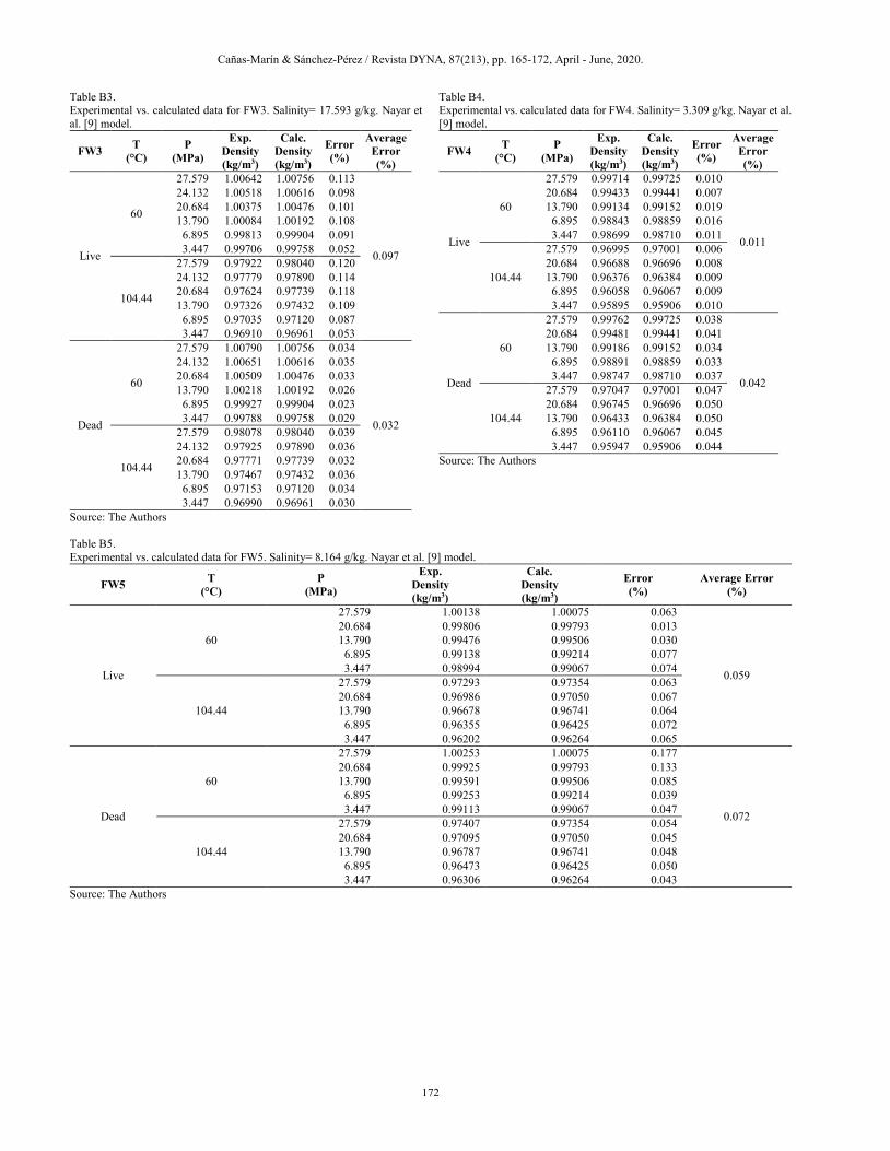
A.1. High pressure Equation of state for seawater, Millero et al [8].
The density of seawater at high pressure according to the equation of state for seawater (EOS-80) is calculated as presented in eq. (3):
𝜌𝜌(𝑆𝑆,𝑇𝑇,𝑃𝑃) =𝜌𝜌(𝑆𝑆,𝑇𝑇, 0)
1 − 𝑃𝑃𝐾𝐾(𝑆𝑆,𝑇𝑇,𝑃𝑃)
(3)
Where 𝜌𝜌(𝑆𝑆,𝑇𝑇, 0) is the density of standard seawater at
atmospheric pressure and is calculated as shown in eq. (4), P is pressure in bars and 𝐾𝐾(𝑆𝑆,𝑇𝑇,𝑃𝑃) is the secant bulk modulus of seawater and is calculated with eq. (5).
- Density of standard seawater at atmospheric pressure:
𝜌𝜌(𝑆𝑆,𝑇𝑇, 0) = (0.999841594 + 6.793952 ∗ 10−5𝑇𝑇 −9.095290 ∗ 10−6𝑇𝑇2 + 1.001685 ∗ 10−7𝑇𝑇3 −1.120083 ∗ 10−9𝑇𝑇4 + 6.536362 ∗ 10−12𝑇𝑇5) +(8.25917 ∗ 10−4 − 4.4490 ∗ 10−6𝑇𝑇 + 1.0485 ∗10−7𝑇𝑇2 − 1.2580 ∗ 10−9𝑇𝑇3 + 3.315 ∗10−12𝑇𝑇4)𝑆𝑆 + (−6.33761 ∗ 10−6 + 2.8441 ∗10−7𝑇𝑇 − 1.6871 ∗ 10−8𝑇𝑇2 + 2.83258 ∗10−10𝑇𝑇3)𝑆𝑆3 2⁄ + (5.4705 ∗ 10−7 − 1.97975 ∗10−8𝑇𝑇 + 1.6641 ∗ 10−9𝑇𝑇2 − 3.1203 ∗10−11𝑡𝑡3)𝑆𝑆2
(4)
- Secant bulk modulus of seawater:

Cañas-Marín & Sánchez-Pérez / Revista DYNA, 87(213), pp. 165-172, April - June, 2020.
171
𝐾𝐾(𝑆𝑆,𝑇𝑇,𝑃𝑃) = 𝐾𝐾0 + 𝐴𝐴𝑃𝑃 + 𝐵𝐵𝑃𝑃2 (5) Where: 𝐾𝐾0 = 𝐾𝐾𝑠𝑠0 + 𝑎𝑎𝑆𝑆 + 𝑏𝑏𝑆𝑆3 2⁄ 𝐴𝐴 = 𝐴𝐴𝑠𝑠 + 𝑐𝑐𝑆𝑆 + 𝑑𝑑𝑆𝑆3 2⁄ 𝐵𝐵 = 𝐵𝐵𝑠𝑠 + 𝑒𝑒𝑆𝑆 𝐾𝐾𝑠𝑠0 = 19652.21 + 148.4206𝑇𝑇 − 2.327105𝑇𝑇2 + 1.360477 ∗
10−2𝑇𝑇3 − 5.155288 ∗ 10−5𝑇𝑇4 𝐴𝐴𝑠𝑠 = 3.239908 + 1.43713 ∗ 10−3𝑇𝑇 + 1.16092 ∗ 10−4𝑇𝑇2 −
5.77905 ∗ 10−7𝑇𝑇3 𝐵𝐵𝑠𝑠 = 8.50935 ∗ 10−5 − 6.12293 ∗ 10−6𝑇𝑇 + 5.2787 ∗ 10−8𝑇𝑇2 𝑎𝑎 = 54.6746− 0.603459𝑇𝑇 + 1.09987 ∗ 10−2𝑇𝑇2 − 6.1670 ∗ 10−5𝑇𝑇3 𝑏𝑏 = 7.944 ∗ 10−2 + 1.6483 ∗ 10−2𝑇𝑇 − 5.3009 ∗ 10−4𝑇𝑇2 𝑐𝑐 = 2.2838 ∗ 10−3 − 1.0981 ∗ 10−5𝑇𝑇 − 1.6078 ∗ 10−6𝑇𝑇2 𝑑𝑑 = 1.9107 ∗ 10−4 𝑒𝑒 = −9.9348 ∗ 10−7 + 2.0816 ∗ 10−8𝑇𝑇 + 9.1697 ∗ 10−10𝑇𝑇2
Units: 𝜌𝜌 in kg/m3, S in kg/m3, T in °C and P in bar. A.2. Seawater density correlation, Nayar et al. [9]. The density of seawater at high pressure according to Nayar et al. [9] is calculated as shown in eq. (6).
𝜌𝜌𝑠𝑠𝑠𝑠(𝑇𝑇, 𝑆𝑆,𝑃𝑃) = 𝜌𝜌𝑠𝑠𝑠𝑠(𝑇𝑇, 𝑆𝑆,𝑃𝑃𝑜𝑜) ∗ 𝐹𝐹𝑃𝑃 (6)
Where 𝜌𝜌𝑠𝑠𝑠𝑠(𝑇𝑇, 𝑆𝑆,𝑃𝑃𝑜𝑜) is the seawater density at atmospheric pressure calculated by using Sharqawy et al. [5] and 𝐹𝐹𝑃𝑃 is the pressure correction factor. The equations to calculate these expressions are shown in eq. (7) and (8) respectively.
𝜌𝜌𝑠𝑠𝑠𝑠(𝑇𝑇, 𝑆𝑆,𝑃𝑃𝑜𝑜) = (𝑎𝑎1 + 𝑎𝑎2𝑇𝑇 + 𝑎𝑎3𝑇𝑇2 + 𝑎𝑎4𝑇𝑇3 + 𝑎𝑎5𝑇𝑇4) +(𝑏𝑏1𝑆𝑆𝐾𝐾𝐾𝐾 𝐾𝐾𝐾𝐾⁄ + 𝑏𝑏2𝑆𝑆𝐾𝐾𝐾𝐾 𝐾𝐾𝐾𝐾⁄ 𝑇𝑇 + 𝑏𝑏3𝑆𝑆𝐾𝐾𝐾𝐾 𝐾𝐾𝐾𝐾⁄ 𝑇𝑇2 +𝑏𝑏4𝑆𝑆𝐾𝐾𝐾𝐾 𝐾𝐾𝐾𝐾⁄ 𝑇𝑇3 + 𝑏𝑏5𝑆𝑆𝐾𝐾𝐾𝐾 𝐾𝐾𝐾𝐾⁄
2 𝑡𝑡𝑇𝑇2)
(7)
Where: 𝑎𝑎1 = 9.999 ∗ 102 𝑏𝑏1 = 8.020 ∗ 102 𝑎𝑎2 = 2.034 ∗ 10−2 𝑏𝑏2 = −2.001 𝑎𝑎3 = −6.162 ∗ 10−3 𝑏𝑏3 = 1.677 ∗ 10−2 𝑎𝑎4 = 2.261 ∗ 10−5 𝑏𝑏4 = −3.060 ∗ 10−5 𝑎𝑎5 = −4.657 ∗ 10−8 𝑏𝑏5 = −1.613 ∗ 10−5
𝑆𝑆𝐾𝐾𝐾𝐾 𝐾𝐾𝐾𝐾⁄ =𝑆𝑆
1000
𝐹𝐹𝑝𝑝 = 𝑒𝑒𝑒𝑒𝑒𝑒 �(𝑃𝑃 − 𝑃𝑃𝑜𝑜) ∗ 𝑋𝑋 +(𝑃𝑃2 − 𝑃𝑃𝑜𝑜2)
2∗ 𝑌𝑌�
(8)
Where: 𝑋𝑋 = 𝑐𝑐1 + 𝑐𝑐2𝑡𝑡 + 𝑐𝑐3𝑡𝑡2 + 𝑐𝑐4𝑡𝑡3 + 𝑐𝑐5𝑡𝑡4 + 𝑐𝑐6𝑡𝑡5 + 𝑆𝑆 ∗ (𝑑𝑑1 + 𝑑𝑑2𝑡𝑡 + 𝑑𝑑3𝑡𝑡2) 𝑌𝑌 = 𝑐𝑐7 + 𝑐𝑐8𝑡𝑡 + 𝑐𝑐9𝑡𝑡3 + +𝑑𝑑4𝑆𝑆
𝑐𝑐1 = 5.0792 ∗ 10−4 𝑑𝑑1 = −1.1077 ∗ 10−6 𝑐𝑐2 = −3.4168 ∗ 10−6 𝑑𝑑2 = 5.5584 ∗ 10−9 𝑐𝑐3 = 5.6931 ∗ 10−8 𝑑𝑑3 = −4.2539 ∗ 10−11 𝑐𝑐4 = −3.7263 ∗ 10−10 𝑑𝑑4 = 8.3702 ∗ 10−9 𝑐𝑐5 = 1.4465 ∗ 10−12 𝑐𝑐6 = −1.7058 ∗ 10−15 𝑐𝑐7 = −1.3389 ∗ 10−6 𝑐𝑐8 = 4.8603 ∗ 10−9 𝑐𝑐9 = −6.8039 ∗ 10−13
Units: 𝜌𝜌𝑠𝑠𝑠𝑠 in kg/m3, t in °C, S in g/kg, P in MPa
Appendix B Table B1. Experimental vs. calculated data for FW1. Salinity= 1.77122 g/kg. Nayar et al. [9] model.
FW1 T (°C)
P (MPa)
Exp. Density (kg/m3)
Calc. Density (kg/m3)
Error (%)
Average Error (%)
Live
87.77
27.579 0.98087 0.98011 0.077
0.071
20.684 0.97789 0.97716 0.074 13.790 0.97488 0.97416 0.074 6.895 0.97178 0.97110 0.069 3.447 0.97024 0.96955 0.071
98.88
27.579 0.97345 0.97275 0.072 20.684 0.97040 0.96973 0.068 13.790 0.96731 0.96666 0.067 6.895 0.96419 0.96352 0.069 3.447 0.96257 0.96193 0.067
Dead
87.77
27.579 0.98110 0.98011 0.101
0.097
20.684 0.97812 0.97716 0.098 13.790 0.97512 0.97416 0.098 6.895 0.97206 0.97110 0.099 3.447 0.97048 0.96955 0.095
98.88
27.579 0.97369 0.97275 0.096 20.684 0.97063 0.96973 0.093 13.790 0.96759 0.96666 0.096 6.895 0.96447 0.96352 0.099 3.447 0.96286 0.96193 0.096
Source: The Authors
Table B2. Experimental vs. calculated data for FW2. Salinity= 2.268 g/kg. Nayar et al. [9] model.
FW2 T (°C)
P (MPa)
Exp. Density (kg/m3)
Calc. Density (kg/m3)
Error (%)
Average Error (%)
Live
87.77
27.579 0.98134 0.98047 0.089
0.086
20.684 0.97841 0.97752 0.091 13.790 0.97535 0.97452 0.086 6.895 0.97230 0.97146 0.086 3.447 0.97072 0.96992 0.082
98.88
27.579 0.97392 0.97311 0.083 20.684 0.97092 0.97010 0.085 13.790 0.96778 0.96702 0.078 6.895 0.96475 0.96388 0.090 3.447 0.96314 0.96230 0.088
Dead
87.77
27.579 0.98144 0.98047 0.098
0.103
20.684 0.97855 0.97752 0.105 13.790 0.97554 0.97452 0.105 6.895 0.97244 0.97146 0.100 3.447 0.97090 0.96992 0.102
98.88
27.579 0.97411 0.97311 0.103 20.684 0.97111 0.97010 0.104 13.790 0.96797 0.96702 0.098 6.895 0.96490 0.96388 0.105 3.447 0.96333 0.96230 0.107
Source: The Authors
Cañas-Marín & Sánchez-Pérez / Revista DYNA, 87(213), pp. 165-172, April - June, 2020.
172
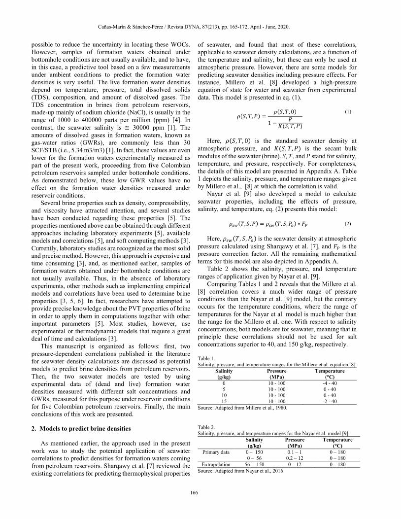
Table B3. Experimental vs. calculated data for FW3. Salinity= 17.593 g/kg. Nayar et al. [9] model.
FW3 T (°C)
P (MPa)
Exp. Density (kg/m3)
Calc. Density (kg/m3)
Error (%)
Average Error (%)
Live
60
27.579 1.00642 1.00756 0.113
0.097
24.132 1.00518 1.00616 0.098 20.684 1.00375 1.00476 0.101 13.790 1.00084 1.00192 0.108 6.895 0.99813 0.99904 0.091 3.447 0.99706 0.99758 0.052
104.44
27.579 0.97922 0.98040 0.120 24.132 0.97779 0.97890 0.114 20.684 0.97624 0.97739 0.118 13.790 0.97326 0.97432 0.109 6.895 0.97035 0.97120 0.087 3.447 0.96910 0.96961 0.053
Dead
60
27.579 1.00790 1.00756 0.034
0.032
24.132 1.00651 1.00616 0.035 20.684 1.00509 1.00476 0.033 13.790 1.00218 1.00192 0.026 6.895 0.99927 0.99904 0.023 3.447 0.99788 0.99758 0.029
104.44
27.579 0.98078 0.98040 0.039 24.132 0.97925 0.97890 0.036 20.684 0.97771 0.97739 0.032 13.790 0.97467 0.97432 0.036 6.895 0.97153 0.97120 0.034 3.447 0.96990 0.96961 0.030
Source: The Authors
Table B4. Experimental vs. calculated data for FW4. Salinity= 3.309 g/kg. Nayar et al. [9] model.
FW4 T (°C)
P (MPa)
Exp. Density (kg/m3)
Calc. Density (kg/m3)
Error (%)
Average Error (%)
Live
60
27.579 0.99714 0.99725 0.010
0.011
20.684 0.99433 0.99441 0.007 13.790 0.99134 0.99152 0.019 6.895 0.98843 0.98859 0.016 3.447 0.98699 0.98710 0.011
104.44
27.579 0.96995 0.97001 0.006 20.684 0.96688 0.96696 0.008 13.790 0.96376 0.96384 0.009 6.895 0.96058 0.96067 0.009 3.447 0.95895 0.95906 0.010
Dead
60
27.579 0.99762 0.99725 0.038
0.042
20.684 0.99481 0.99441 0.041 13.790 0.99186 0.99152 0.034 6.895 0.98891 0.98859 0.033 3.447 0.98747 0.98710 0.037
104.44
27.579 0.97047 0.97001 0.047 20.684 0.96745 0.96696 0.050 13.790 0.96433 0.96384 0.050 6.895 0.96110 0.96067 0.045 3.447 0.95947 0.95906 0.044
Source: The Authors
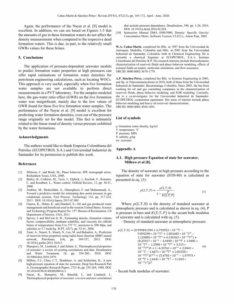
Table B5. Experimental vs. calculated data for FW5. Salinity= 8.164 g/kg. Nayar et al. [9] model.
FW5 T (°C)
P (MPa)
Exp. Density (kg/m3)
Calc. Density (kg/m3)
Error (%)
Average Error (%)
Live
60
27.579 1.00138 1.00075 0.063
0.059
20.684 0.99806 0.99793 0.013 13.790 0.99476 0.99506 0.030 6.895 0.99138 0.99214 0.077 3.447 0.98994 0.99067 0.074
104.44
27.579 0.97293 0.97354 0.063 20.684 0.96986 0.97050 0.067 13.790 0.96678 0.96741 0.064 6.895 0.96355 0.96425 0.072 3.447 0.96202 0.96264 0.065
Dead
60
27.579 1.00253 1.00075 0.177
0.072
20.684 0.99925 0.99793 0.133 13.790 0.99591 0.99506 0.085 6.895 0.99253 0.99214 0.039 3.447 0.99113 0.99067 0.047
104.44
27.579 0.97407 0.97354 0.054 20.684 0.97095 0.97050 0.045 13.790 0.96787 0.96741 0.048 6.895 0.96473 0.96425 0.050 3.447 0.96306 0.96264 0.043
Source: The Authors