Prediction of Flow-Rate of Sanaga Basin in Cameroon

Energy and Environment Research; Vol. 2, No. 1; 2012 ISSN 1927-0569 E-ISSN 1927-0577

Published by Canadian Center of Science and Education

205

Prediction of Flow-Rate of Sanaga Basin in Cameroon Using HEC-HMS Hydrological System: Application to the Djerem

Sub-Basin at Mbakaou

Serge Herve Boyogueno1, Michel Mbessa2 & Thomas Tamo Tatietse2 1 Faculty of Science, University of Yaoundé I, Yaounde, Cameroon 2 National Advanced School of Engineering, University of Yaoundé I, Yaounde, Cameroon

Correspondence: Serge Herve Boyogueno, Faculty of Science, University of Yaoundé I, Yaounde, P.O. Box 812, Yaounde, Cameroon. Tel: 237-99-413-093 & 237-76-293-495. E-mail: [email protected]

Received: October 21, 2011 Accepted: November 8, 2011 Online Published: May 29, 2012

doi:10.5539/eer.v2n1p205 URL: http://dx.doi.org/10.5539/eer.v2n1p205

Abstract

This article proposes the development of a rainfall-runoff model in order to simulate the hydrologic behavior of the Djerem sub-basin at Mbakaou in the Sanaga basin in Cameroon. We suggest a solution based on a spatial conceptual modeling, then a restriction to a finite number of parameters judged applicable for the different choices of models. The approach relies on the hydrologic system HEC-HMS whose interest is not only it's adaptability to the tropical and equatorial climate, but also and especially to the acceptable results that it provides for a very weak quantity of data. In this work, we take into consideration the different aspects of modeling such as: surface flow, underground flows, direct runoffs, losses, as well as interactions between the surface and the base-flow of rivers. The results obtained allows the planning of the Mbakaou dam, consequently to increase the hydroelectric production on one hand and on the other hand, provide some exploitable information for dimensions of hydrologic works, protective against floods or for hydrologic management and ecology of the Djerem basin at Mbakaou. To validate our model, a comparison of the simulated flow-rate and the observed flow-rate was carried out using historic data with the Nash-Sutcliffe Criterion and we obtained an efficiency of 0.862, meaning that the simulation was good.

Keywords: rainfall-runoff, basin, modeling, spatial, hydrologic system

1. Introduction

In Cameroon, the production of electric energy is assured by well developed hydraulic and minor thermal systems. The production of quasi - total electric energy of hydraulic origin on the Sanaga River is achieved through two hydroelectric power stations: Edéa and Song-Loulou.

The flow-rate of water nourishing these power stations depend directly on the natural flow of the Sanaga river but this flow-rate varies from 8000 m3/s in rainy seasons to less than 200 m3/s in the dry season. With the objective to regulate this flow-rate, the Sanaga has been equipped with three storage dams (Mbakaou, Bamendjin, Mapé) that are unfortunately very distant from the power production stations (see Figure 1), posing the following enormous problems on the entire Sanaga basin:

Difficulties at the level of hydrologic follow-up and forecasting of the inflows on the entire basin;

Propagation time varies from 5 to7 days between reservoirs and power stations;

Production losses associated to the difficulty of predicting flow to power stations and to plan the manipulation of storage dams;

Improvement of performance indicators at the level of the production.

To assure a good exploitation of the water in the storage dams, we must predict in advance, inflow at the level of the storage dams. The natural flow-rate of the Sanaga to the length of propagation time, in order to release just the necessary quantity of water thereby maintaining the flow-rate in the production factories of the value required to assure the electric power called to the boundary of alternators.

www.ccsenet.org/eer Energy and Environment Research Vol. 2, No. 1; 2012

206

The consideration of the above mentioned problems is necessary and indispensable because they greatly influence the regulation of the Sanaga River.

The mastery of all these problems allows us to better plan the manipulation at the level of storage dams, thus increasing the production of hydroelectric energy and reducing the costs of thermal plants which compliments hydroelectric energy.

Figure 1. System of hydroelectric energy production of the basin of the River Sanaga

(Source: GridDispatch, 2011)

Our problem statement is situated in the framework of a rainfall - runoff model development with the daily time step allowing the assessment of a rainfall data, inflow of water into the outlet of the Djerem sub-basin at Mbakaou. It is about implementing a GIS data base of our basin, choosing parameters for the different models (subsurface flows, surface flows, direct runoff, losses, evapotranspiration and rainfall) according to the available data then; we simulate and calibrate these models. It permits us to obtain a hydrograph at the level of the storage dam of Mbakaou. The objective of this article is to allow prediction engineers to master the inflows of water into the storage dams and to better plan the exploitation of these dams.

2. Principle of the Present Regulation of the Sanaga River

A target regulated flow-rate QTR at an instant is fixed in order to satisfy the production of energy demanded. We make forecasts with a default rate of 25% on the flow-rate of the intermediate basin QIB, to view its evolution during the previous years. We determine the corresponding flow-rate to be released QR while taking in to account the losses by infiltration and by evaporation (10% of the released flow-rate) (Grid Dispatch, 2011).

This flow-rate to be released at a time t can be modeled by the following equation:

QR = (QTR – QIB) ×1,1 (1)

The flow-rate of the intermediate basin (QIB) is a function of the subsurface inflow and rain-gauge of the intermediate sub-basin (Dkengne, 2006). This flow-rate is actually determined by forecasting at a time t by the exponential law of drop in level as follows:

Q(t) = Q0 ×e-t/T (2)


207

Where:

Q(t) is the projected flow-rate of the intermediate sub-basin at a date t;

Q0 is the daily flow-rate of the intermediate basin;

T is the reference time: T=24 days when t < 24 days;

T=49 days when (24 < t < 49) days;

T=79 days when (49 < t < 79) days.

The propagation duration of discharges from the dams to the production site along the Sanaga, is about one, thus the reference time considered is 24 days.

After setting the target flow-rate required, meeting the production forecast and finding the flow-rate of the intermediate basin, the hydrological operating service Grid-Dispatch determines the corresponding flow-rate released. The volume to be released is partioned and instructions are then sent to the various dams. Communication is provided by radio wave VHF. Finally, the flow-rate is measured at the reference hydrologic station Sombengué which is compared to the required flow-rate.

2.1 The Deficiencies of the Current System

The lack of reliable measurement station upstream and downstream at the production plants, thereby causing discrepancies between production capacity and the flux of turbine water.

The insufficient number of hydro-rainfall monitoring stations (only 10 stations are actually being operated on the entire basin) and their uneven distribution on the Sanaga watershed.

Unreliable rainfall predictions for the intermediary watershed during the propagation time of discharges from the dam to Song-Loulou.

The lack of effective planning for maintenance, calibration and monitoring of the hydrometric network stations.

The unavailability of reliable hydrological software for data collection, validation, processing, storage and management to ensure better achievements and search of reliable data for different applications.

Due to many of these imperfections, the target regulated flow in low water can only be guaranteed with a failure rate of about 25% (that is to say for four forecasts, one is wrong).

During the first phase of the dry season between December 1 and March 15, when the water level drops due to the absence of rainfall, flow forecasts follow the law of recession and the values obtained are more or less reliable. During the second phase of the dry season, from March 15 to June 15, characterized by a short rainy season, the forecasts are no longer reliable and operational losses are significant, simply because of the difficulty to take into consideration forecasts of precipitation 5 to 7 days in advance as required by this method.

2.2 The Advantage of a Mathematical Model for the Regulation of the Sanaga

The whole point of a mathematical model is therefore to reconcile the exigencies of meeting the demand for energy and to limit losses by dumping. The objective being to ensure proper flow control in low water with a failure of the order of 5% by using optimal management of water stored and the input at the level of reservoir dams.

To produce hydroelectric power, both flow-rate and a drop height are required. This flow-rate can be determined using the rain-gauge and this using a mathematical model: rainfall-runoff model like the water system such as HEC-HMS. The formula below calculates the electrical power:

P(MW)= ρ×g×μ×Qt×H(m) (3)

Where:

P: electrical power (MW), ρ: Density of water (Kg/m3), g: Acceleration due to gravity (m/s2), μ: performance of turbine alternator, Qt: turbine flow-rate (m3/s) and H: Height of fall (m) (GridDispatch, 2011).

3. Material and Methods

The new contribution brought in after this summary presentation of the present principal method of regulating the River Sanaga, will contribute to the amelioration of the management of storage dams.


208

3.1 Mathematical Modeling: Rainfall-runoff

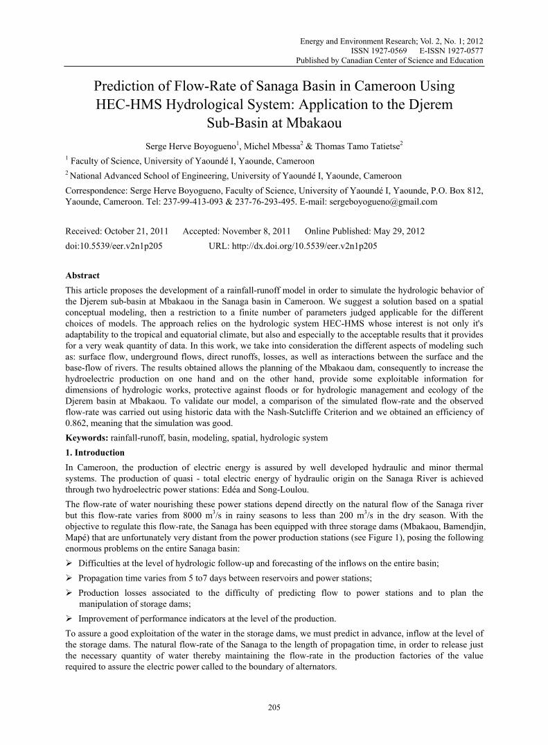
The design of this model is deduced from the hydrological cycle as shown in Figure 2, and hydrological balance (Equation 4). This formulation takes into account all elements involved in the transformation of rainfall into runoff.

With, P=Precipitation; R=surface flow; G=Underground flow; E=Evaporation; T=Transpiration

Figure 2. The hydrologic cycle (Henine, 2004)

For a given time interval, the mathematical model of the hydrological balance of Figure 2 is written as follows (taking into account all components of the hydrological cycle in units of height):

P – R – G – E – T = ΔS (4)

With, ΔS = Variation of stocking.

3.2 Rainfall-runoff Model Using the HEC-HMS Hydrological System

The HEC-HMS System (Hydrologic Modeling System) is software that simulates the hydrological behavior of a watershed due to predetermined rain events, developed by Hydrologic Engineering Center (HEC) of the Corps of Engineers of the U.S. Army. The program has a graphical interface, integrated hydrologic components, a specific system of data storage (DSS) and management tools, etc.

Modeling the response of a watershed subject to a phenomenon in the system with HEC-HMS (Scharffenberg et al, 2010) is divided into three parts: modeling the basin, modeling of meteorology and particular specifications.

3.2.1 Modeling of the Basin

The Modeling of a watershed consist, at first in partitioning it into several basic sub-watersheds (Ford et al., 2008), then specifying the methods used to calculate the infiltration, runoff and underground water flows.

Dividing the Djerem basin at Mbakaou into several sub-basins

The mapping of a watershed into sub-basins is carried out using the software GeoSFM. They are extensions of ArcView Geographic Information System and Spatial Analyst (Fewsnet & Debbie, 2006). These extensions produce a number of hydrological inputs which are directly employed by HEC-HMS. They assist the user to assess hydrological parameters by providing tables of the physical characteristics of streams and sub-basins (see Tables 2 & 3). It also allows users to view spatial information, characteristics of the watershed to delineate sub-basins, streams, etc.

The basin is divided into several sub-basins bounded by water dividing lines. Each is represented by an element called "sub-basin". It contains all the necessary physical and hydrological parameters for simulation which are: the surface and the name of the sub-basin, the methods of calculating "loss", the "runoff" and "groundwater flow". Just like sub-basins, the rivers are also modeled and represented by hydrologic features called "reach" each containing the method describing their transfer function and the necessary information for the latter such as: The type of equivalent surface (spherical or prismatic), the length, the Manning coefficient, etc. It may also include mapping of reservoirs in the watershed, they are represented by the element 'Reservoir'. All these elements must be connected to form a network by including sub-basin, reach, junction, reservoir, diversion, source and sink (see Figure 9). The extraction procedure of drainage and delineation of the watershed into 22 sub-basins is summarized in the Figures 3, 4, 5, 6, 7 and 8.


209

Figure 3. DEM of Africa of 1Km×1Km resolution (Zobler, 1986)

Figure 4. Delineation of DEM of the Djerem basin at Mbakaou, correction of certain errors of DEM

Figure 5. Correction of DEM by the replacement of depression in increasing the altitude of cells at the level of the environmental field in order to determine the direction of flow

Figure 6. Definition of the direction of flow following a certain number of possible directions


210

Figure 7. Definition of rivers: This step classifies all cells of which the accumulation of out-flow is greater than a given threshold

Figure 8. Delineation of the sub-basins: This step traces the limits of sub-basins for every river segment. Considering the size of our basin (20 200 Km²), It was not possible to subdivide it in less than 22 sub - basins

Figure 9. Final Representation of the basin model in HEC-HMS (subdivided into 22 sub-basins)


211

Modeling losses

The flow volumes are calculated by subtracting from rainfall, the quantity of water stored, infiltrated or evaporated in the watershed. The interception, infiltration, storage and evaporation are shown as "loss". We use a model called the initial loss at constant rate.

This model assumes that the potential maximum loss rate, denoted fc is constant, and includes the rate of initial losses Ia representing the interception and storage in surface depressions. The interception is a consequence of the absorption of rain by vegetation cover and surface storage is the result of the topography of the watershed: the water stored in surface depressions will be evaporated or infiltrated. So long as Ia is not reached, there is no runoff. Its operation is summarized as follows:

If i i aP I then Pet = 0

If i i aP I and t cP f then et t cP p f (5)

If i i aP I and t cP f then 0etP

Where, Pt: mean areal precipitation at time t; Pet: the runoff at time t given by:

(6)

If the soil of the watershed is saturated, Ia will be close to zero. If the soil is drained, then Ia represent the amount of water that falls on the watershed with no run-off. This amount is based on the nature of land in the watershed, land use, type and use of ground. As a guide, it is estimated that these losses are equal to 10 or 20% of the total rainfall for a forest, while in urban areas they are between 2 and 5 mm of water height.

Modeling of direct runoff

The process we refer here is the conversion of excess rainfall for each sub-basin in a flow at its outlet. We use an empirical model named Clark Model which uses a unit synthetic hydrograph. The two processes involved in the transformation of excess precipitation into runoff, i.e. the movement of water from its origin to the outlet of the watershed and the reduction of this amount of water by storing in its way are included here.

Modeling groundwater

We have used here the Nonlinear Boussinesq Baseflow model for the availability of its parameters such as porosity, conductivity, the length of the river, etc…

On each stream contained in each sub-basin, the following phenomena are taken into account:

i. Modeling of losses or gains

This model allows us to take into account channel losses, additions of underground water to the channel, or the two-way movements of water.

ii. Modeling of river flow

We calculate a hydrograph downstream of the watershed, knowing the upstream hydrograph, using the equations of continuity and momentum. The model called Muskingum has been used for this purpose.

This model uses a simple finite difference approximation of the continuity equation:

1 1 1( ) ( ) ( )2 2

t t t t t tI I O O S S

t

(7)

It is then expressed that the volume of water stored is the sum of a constant volume stored and a change in stock

St = TpOt + TpX(It - Ot) = Tp (XIt + (1 - X)Ot) (8)

With, Tp: Travel time and a weighting parameter for X (0<X<0.5).

Thus, if the storage of water in the river is controlled by downstream conditions, we put X = 0. Instead, we will take X = 0.5, to give a weight similar to the flows into and out. Finally, we obtain the following equation:


212

1 1

2 2 2 (1 )( ) ( ) ( )2 (1 ) 2 (1 ) 2 (1 )

p p pt t t t

p p p

t T X t T X T X tO I I O

T X t T X t T X t

(9)

Knowing the values of Tp, X, ∆t for all times t, and the initial condition (O0). The system HEC-HMS calculates by induction the upstream hydrograph.

The parameters Tp and X can be obviously estimated by a series of trial and error corrected progressively. Tp can also be measured as the time interval between two similar points belonging respectively to upstream and downstream hydrographs.

3.2.2 Meteorologic Modeling

Modeling of the rainfall

We used data from five rainfall stations that were likely to influence the flow in ourwatershed. Then we calculated the mean areal precipitation (Pmoy). It is obtained by the arithmetic mean after you assign a weight for each station:

( ( ))i ii Tmoy

ii

W P tP

W

(10)

Where, Wi: weight factor assigned to gauge/observation i and Pi(t): precipitation depth measured at time t at gauge i.

Finally the weighting factor (Wi) assigned to gauge i is calculated using the method of Thiessen polygons:

ijj

i

aW

A (11)

With:

aij: surface intersection of the « polygon j » and « sub-basin i » ;

Ai: total area of sub-basin i.

The results are shown in Table 1.

Table 1. Rain-gauge Stations and coefficients values of the polygon of Thiessen

Stations Latitude Longitude Altitude in m Coefficient de Thiessen (Wi )

Banyo 06°44’00’’ 11°48’00’ 1110 6,25%

Meiganga 06°31’00’’ 14°17’00’ 1027 17,18%

Ngaoundere 07°19’00’’ 13°35’00’ 1138 31,95%

Tibati 08°28’00’’ 12°37’00’ 874 33,98%

Tignere 07°23’00’’ 13°39’00’ 1160 10,65%

Evapotranspiration Modeling

We used the «THORNTHWAITE» formula presented below to calculate evapotranspiration from the values of temperature of four of the five precedingstations, except the station of Tignere.

10 ( )( ) 16[ ] ( , )aT m

ETP m F mI

(12)

With:

ETP(m): monthly average evapotranspiration m (m=1 à 12) in mm;

F(m,φ): monthly corrective Factor function m and latitude φ;

T(m): average monthly temperature in C;

I: Annual heat index, defined as :


213

12( )

mI i m ; 1.514( )

( ) [ ]5

T mi m (13)

a = 0.016 × I + 0.5

3.2.3 The Control Specifications

They help to define the starting time and the end of time of the simulation and the time step of calculation. Time steps can vary between 1 and 24 hours.

3.2.4 Parameterization, Simulation and Calibration of Rainfall-runoff Model

Parameterization

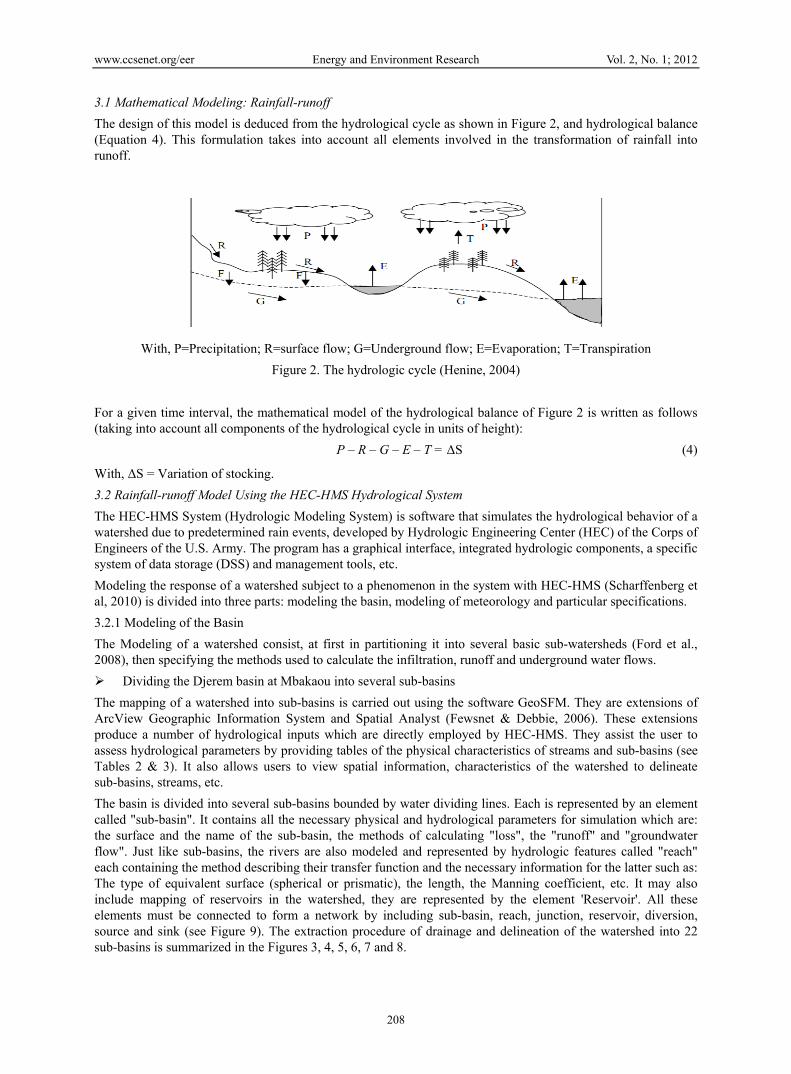
The procedure for schematization of the Djerem Basin at Mbakaou in ArcView, leads to the calculations results of physical quantities of the various ponds and bays in tables. These different sizes will be used to parameterize our model.

Table 2. Physical Characteristics of the different sub-basin

Table 3. Physical characteristics of the different reach

Simulation

We used rainfall data from the stations Banyo, Meiganga, Ngaoundere, Tibati and Tignere, with capital flows measured at the outlet of our watershed and finally the values of the physical characteristics of the basin and table of contents 2 & 3. After the first simulations in the year 1989, we have calibrated the model with the years from 1990 to 2001 to finally validate the model in the year 2002, so the result is shown in Figure 11.

Calibration

In our model, we used some parameters that cannot be estimated by observation or by measuring the channel characteristics and watershed. For example, the parameter X in the Muskingum model cannot be measured because it is simply a weight that indicates the relative importance of the flow up and down by calculating the storage in the channel of the stream. How then can the appropriate values of the parameters be chosen? If the observations of precipitation and runoff are available, then the calibration is the answer. The calibration uses hydro-meteorological observational data in a systematic search for parameters that yield the best fit of calculated


214

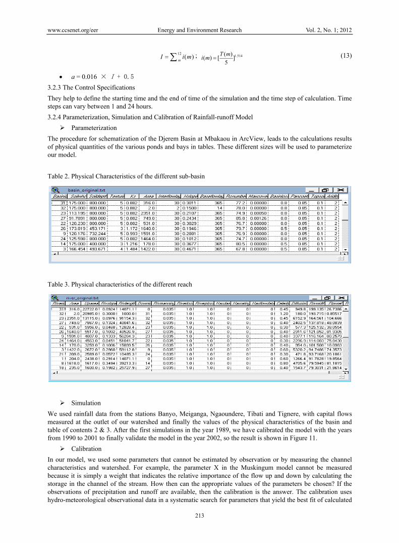
results for the observed runoff. This research, known as "optimization" has allowed us to find the optimal values of some of our parameters. We used the principle described in Figure 10.

Figure 10. Diagram of the calibration process (Feldman, 2000)

With objective function, the function (Z) defined by

01( ) ( )

NQ

siZ q i q i

(Stephenson, 1979) (14)

With: Z = the objective function; NQ = number of ordinates of calculated hydrograph

q0(t) =observed flow-rate; qs(t) = calculated flow-rate.

4. Results and Comments

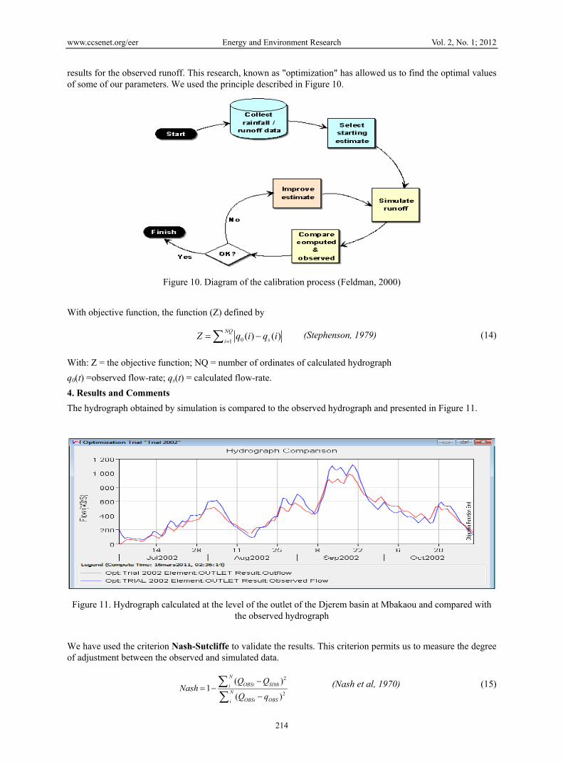
The hydrograph obtained by simulation is compared to the observed hydrograph and presented in Figure 11.

Figure 11. Hydrograph calculated at the level of the outlet of the Djerem basin at Mbakaou and compared with the observed hydrograph

We have used the criterion Nash-Sutcliffe to validate the results. This criterion permits us to measure the degree of adjustment between the observed and simulated data.

2

2

( )1

( )

N

OBSi SIMiiN

OBSi OBSi

Q QNash

Q q

(Nash et al, 1970) (15)


215

With, QOBSi and QSIMi respectively being the observed flow-rates and simulated with the time step i, and N the total number of time step of the study period; qOBS the mean observed flow-rate.

And -∞<Nash≤ 1

If Nash=0; bad simulation;

If Nash>0.7 good simulation;

If Nash=1 perfect Simulation

The value of the Nash criterion for the simulation of the Djerem basin at Mbakaou is 0.862. This means that we have a very good simulation that approximates reality.

From the above, the simulated hydrograph is similar to that observed, yet how to observe the flow of supply reservoirs does not seem reliable because of the discrepancy that may exist between the observed and the reality. For this we propose that in addition to humans, the various observation posts should be equipped with automatic recording device.

A field validation of parameters obtained by satellite images (parameters in Figures 6 & 7), would have allowed us to obtain more reliable results.

We also put an emphasis on data collection that proves to be the most important point of all hydrological modeling. For this, a densification of rain-gauges in the Sanaga basin would be necessary.

The study of phenomena such as infiltration and evapotranspiration will also be interesting to see how they affect the flow.

A densification (rehabilitation and creation) of the river system will allow an understanding and optimal management of resources.

All these measures will contribute to the amelioration of the outlet results of our sub-basin.

5. Discussion and Conclusion

The mathematical modeling is an essential tool in understanding the processes and dynamic interactions between environmental and physiographic parameters put in place in a hydro-system (Singhy, 1997). In this study, we developed a rainfall-runoff model that can help us to know for a given rainfall, the flow–rate at the outlet of a watershed. This model was developed from HEC-HMS hydrological system, with physical and hydro-meteorological parameters of the studied watershed, and exploitation in data synergy of remote sensing and GIS. All these allow us to build up a geospatial database and to undertake outflow modeling of the Djerem basin at Mbakaou. Such a system has the advantage of producing acceptable results with a very small amount of data.

The simulation results (Calage and verification) at the Mbakaou station, which is more downstream, shows a good synchronism between simulated and observed flows, as shown by the high values of the Nash criteria (0.862). However, at certain stations upstream, the speed of the curves is not synchronous at certain levels. We observe an under estimation and at times an over estimation on one part of the hydrologic cycle. These discrepancies seem to be due to an extrapolation problem of the Calage parameters but reveal also the incapacity (inability) of the network of precipitation measurements to follow their spatio-temporal distribution on this sub basin. Otherwise, when rain is isolated and of weak extension, their extrapolation drives to results that contain curves between simulations. Besides the reinforcement of the network measurements of the meteorological variables, radar images can contain a good source of data for spatialization of rainy events.

This study should enable the company responsible for the production of electricity in Cameroon, not only to plan the maneuvers on dams and reservoirs and to reduce the cost of heat, but also and especially to increase the production of hydroelectric power.

Acknowledgements

We would like to thank all those who from far and near took part in the drafting of this article, particularly the hydrologic division team of AES-SONEL and the UMMISCO laboratory of the Faculty of Sciences, University of Yaounde 1.

References

Dkengne, S. P. (2006). Modélisation et prévision des débits naturels journaliers du B.V.I. de la Sanaga à la station de contrôle de Songmbengue. Mémoire de Master de Statistique Appliquée, ENSP, Yaoundé.


216

Feldman, A. D. (2000). Hydrologic Modeling System: HEC-HMS. Technical Reference Manual. U.S. Army Corps of Engineers, Institute for Water Resources, Hydrologic Engineering Center. Davis, CA. USA.

Fewsnet, I., & Debbie, E. (2006). Geospatial Stream Flow Model (GeoSFM). User’s Manual, version 1.0. Training Center, U.S. Geological Survey Center for Earth Resources Observation and Science (EROS). Sioux Falls, South Dakota, USA.

Ford, D., Pingel, N., & Devries, J. J. (2008). Hydrologic Modeling System: HEC-HMS. Applications Guide. U.S. Army Corps of Engineers, Hydrologic Engineering Center. Davis, CA. USA.

GridDispatch. (2011). Rapport des prévisions hydrologiques et de la production des années antérieures. Rapport de mission. AES-SONEL, Douala.

Hamatan, M. (2007). Procédure de compilation du modèle Hydrologique GeoSFM: Application au Bassin Versant de la SIRBA. Séminaire de formation. CRH, Yaoundé.

Henine, H. (2004). Interfaçage entre un modèle hydrologique / modèle hydrodynamique Au sein d’un système d’information intégré sous web incluent les SIG. Mémoire de magister en hydraulique. ENP, Algérie.

Scharffenberg, W. A., & Fleming, M. J. (2010). Hydrologic Modeling System: HEC-HMS. User’s Manual, Version 3.4. U.S. Army Corps of Engineers, Institute for Water Resources, Hydrologic Engineering Center. Davis, CA. USA.

Zobler, L. (1986). A world soil files for global climate modeling. NASA Technical MEMO 87802-1986. Retrieved from ftp://daac.gsfc.nasa.gov/data/inter_disc/hydrology/soil/

Prediction of Flow-Rate of Sanaga Basin in Cameroon

Documents

Transcript of Prediction of Flow-Rate of Sanaga Basin in Cameroon