1

Prediction of chameleonic efficiency Laurent David,[b] Mark Wenlock,[c] Patrick Barton,[d] and Andreas Ritzén*[a] [a] Dr. A. Ritzén

Drug Design, LEO Pharma A/S, Industriparken 55, 2550 Ballerup, Denmark Present address: Monte Rosa Therapeutics AG, Aeschenvorstadt 36, CH 4057 Basel, Switzerland E-mail: aritzen@monterosatx.com ORCID: 0000-0002-3313-3753

[b] Dr. L. David Computational chemistry, H. Lundbeck A/S, Ottiliavej 9, 2300 Valby, Copenhagen, Denmark

[c] Dr. M. Wenlock Physical Chemistry, Cyprotex Discovery Limited, Alderley Park, Nether Alderley, Cheshire, SK10 4TG, UK

[d] Dr. P. Barton Evotec (UK) Ltd., 114 Innovation Drive, Milton Park, Abingdon, Oxfordshire OX14 4RZ, UK Present address: DMPK, UCB Celltech, branch of UCB Pharma S.A., 208 Bath Road, Slough, Berkshire, SL1 3WE, UK

Abstract: Chameleonic properties, i.e., the capacity of a molecule to hide polarity in non-polar environments and expose it in water, help achieving sufficient permeability and solubility for drug molecules with high MW. We present models of experimental measures of polarity for a set of 24 FDA approved drugs (MW 405 – 1113) and one PROTAC (MW 1034). Conformational ensembles in aqueous and non-polar environments were generated using molecular dynamics. A linear regression model that predicts chromatographic apparent polarity (EPSA) with a mean unsigned error of 10 Å2 was derived based on separate terms for donor, acceptor, and total molecular SASA. A good correlation (R2 = 0.92) with an experimental measure of hydrogen bond donor potential, Dlog Poct–tol, was found for the mean hydrogen bond donor SASA of the conformational ensemble scaled with Abraham’s A hydrogen bond acidity. Two quantitative measures of chameleonic behaviour, the chameleonic efficiency indices, are introduced. We envision that the methods presented herein will be useful to triage designed molecules and prioritize those with the best chance of achieving acceptable permeability and solubility.

Introduction

Simultaneously achieving adequate aqueous solubility and membrane permeability is a challenge for drugs with high molecular weight. Qualitatively, the ability of a molecule to expose polar groups in aqueous environment and hiding polarity in the cell membrane interior by intramolecular hydrogen bond (IMHB) formation can mitigate this issue and help strike an appropriate balance. [1] The term “chameleonic behaviour” has been applied to characterize such solvent-dependent effects, and there are suggestions in the recent literature that molecules above a certain size must be chameleonic to allow sufficient solubility and permeability to function as oral drugs. [2] Many contemporary drug targets and modalities, e.g., viral protease inhibitors, protein-protein interaction modulators, and PROTACs, appear to require ligands with MW > 500. Thus, it is of great interest to develop methods that test for and quantify chameleonic behaviour, and experimental methods, e.g., EPSA [3, 4] and the difference in log P between 1-octanol/water and hydrocarbon/water (Dlog Poct–alk) [5, 6, 7] are useful for the study of effective polarity and hydrogen bonding. Recently, Lokey et al proposed a lipophilic permeability efficiency metric based on the study of a congeneric group of cyclic peptides. [8] Although useful to characterize existing

compounds, these methods do not allow for the prediction of chameleonic behaviour to prioritize new molecules for synthesis. To begin to address this issue we recently reported a molecular dynamics (MD) protocol that was used to derive conformational ensembles from simulations in explicit water and octane. [9] We found that explicit solvent MD qualitatively predicts the increased number of IMHB formed in octane compared with water. In the present study, a set of 25 molecules was compiled consisting of 8 FDA approved drug molecules with MW 400-700, 16 FDA approved drug molecules with MW > 700, and one PROTAC molecule. The molecules cover both synthetic drugs and natural products, and several macrocyclic compounds are included. The structures of the molecules are shown in Figure 1. Because of the recent surge in approvals of HCV NS3/4A and NS5A inhibitors, these classes are dominating the set of molecules with MW > 700. All compounds except the PROTAC are FDA approved oral drugs with systemic action, and they are thus assumed to possess sufficient permeability to be absorbed across cell membranes. To enable modelling of relevant experimental measures of hydrogen bond exposure and polarity, we measured log D in three aqueous/organic systems, and we used the EPSA chromatographic method to determine the effective polarity of the approved drugs in the set of molecules shown in Figure 1.

2

Figure 1. Structures and mechanisms of action of the 24 drug molecules and one preclinical PROTAC studied in this work.

3

Figure 1. continued

Results and Discussion

Conformation-dependent hydrogen bonding potential: Scaled polar surface area Permeability through lipid bilayers involves desolvation of the diffusing molecule as it enters the membrane interior, and once inside the membrane, disengagement from the polar head groups of one leaflet followed by diffusion across the lipid interior, and the reverse process once the molecule reaches the opposite leaflet. [10, 11] Hydrogen bonding is arguably the major contributor to the energy barriers of these desolvation and disengagement events, and the overall hydrogen bonding potential of the molecule should be considered to diagnose passive permeability limitations. The polar surface area (PSA) of a molecule is widely applied in medicinal chemistry as one of the most important parameters for

prediction of permeability. It is defined as the van der Waals surface area (vdW SA, see Figure 2 for definitions) of the nitrogen and oxygen atoms of the molecule, and any hydrogen atoms directly bound to nitrogen and oxygen. Thus, PSA can be considered an approximate measure of the total hydrogen bonding potential of the molecule. Since PSA is calculated from the 3D structure of the molecule, a relevant conformation must first be generated. For flexible molecules, many conformations are possible, and the PSA is therefore not completely unambiguous. To avoid having to generate multiple conformers and decide on which one(s) to use for the PSA calculation, the topological polar surface area (TPSA) parameter is often used as an approximation of the actual PSA. [12] TPSA is based on a look-up table and uses the 2D structure of the molecule. Thus, TPSA does not take conformational effects, e.g., IMHB formation, into account. This makes TPSA flawed for the analysis of chameleonic molecules, where the surface polarity is environment dependent. However, even calculating PSA from the 3D structure of a representative conformer does not accurately reflect the hydrogen bonding potential of the molecule because it ignores the

4

fact that hydrogen bond donor (HBD) and hydrogen bond acceptor (HBA) strengths vary widely between different functional groups, even though the surface area of the heteroatoms are similar. [13] To improve upon the PSA parameter, Platts proposed that scaling the PSA by the hydrogen bonding strengths of the respective polar atoms would yield a better descriptor of polarity. [14] Indeed, this was shown to drastically improve the prediction of partition coefficients in three solvents relative to unscaled PSA. Platts used a single conformer of each molecule, and Abraham’s A and B scales for hydrogen bond donors and acceptors respectively. [15, 16] Since the relative contributions of donors and acceptors to log P is expected to vary between solvents, donors and acceptors were individually summed and the donor and acceptor sums were used to build a multiple linear regression (MLR) model of log P.

Figure 2. Definition of the molecular surface areas. A hypothetical molecule is shown with atomic van der Waals radii as dotted circles. The solid blue envelope is the van der Waals surface area (vdW SA), and the orange outline is the solvent-accessible surface area (SASA). The SASA is constructed by rolling a probe sphere (orange circle, radius = 1.4Å) over the vdW SA and taking the centre of the probe at each position.

As we were interested in computing the conformation-dependent hydrogen bonding potential of a given conformer of a chameleonic molecule, we set out to implement the Platts scaled PSA method with a few modifications: The pKBHX scale [17] for hydrogen bond acceptors was used instead of Abraham’s B scale because it covers many more functional groups, and the scaling calculation was modified as follows. (For a detailed discussion of hydrogen bonding acceptor scales the reader is referred to [18]). Platts multiplied the vdW SA of each nitrogen and oxygen atom with Abraham’s B parameter, and similarly the vdW SA of each hydrogen atom bonded to N or O with Abraham’s A parameter. However, Abraham’s A and B parameters are derived for the polar groups of entire (monofunctional) molecules, thus, multiplying them with atomic surface areas does not produce a physically relevant number. To capture the partial shielding of polar atoms that results from e.g., IMHB formation, we instead multiplied the exposed fraction of the surface area of each polar atom with the respective hydrogen bonding strength (Abraham’s A or pKBHX). Both the vdW SA and the solvent-accessible surface area (SASA, see Figure 2 for definitions) were considered. The exposed fractions were calculated from the exposed surface area divided by values from a look-up tables of the maximum exposed areas of each atom type in a representative compound, see the Experimental section and Supporting information Tables S1 and

S2. The scaled hydrogen bond acceptor surface area is given by Equation 1 and the scaled donor surface area is given by Equation 2. !!"# = ∑ $%&!"#,%'(.*+,%

,&'(,%- (1)

!!". = ∑ #),)

,&'(,)/ (2)

where Si and Sj are the surface areas (vdW SA or SASA) of HBA atom i and HBD atom j respectively, Smax,i and Smax,j are the corresponding maximum possible surface areas for unobstructed atoms from the lookup tables (see Supporting Information Tables S1 and S2), and pKBHX,i and Aj are acceptor and donor (Abraham’s A scale) strengths. Unlike Abraham’s A scale, which can only take positive values, very weak acceptors have negative values on the pKBHX scale. To shift this scale such that weak acceptors have values close to zero, an offset of 0.5 was included. It was selected to achieve a high R2 with a minimum of outliers when used to fit the data to Equation 3, see below. A sensitivity analysis of the impact of changes to this offset on the MLR statistics showed that its value was not critical. A logical test was added to replace negative values of (pKBHX,i + 0.5) with zero, such that no atomic contribution to the scaled hydrogen bond acceptor surface area would be negative. With these modifications, we selected a training set with measured log P (cyclohexane/water) consisting of 98 molecules from the Platts dataset of 110 molecules [14] with the addition of anisole. Phenols are over-represented in the Platts set (26 of the 110 compounds), and six were removed to reduce bias. Three trialkyl phosphates and three charged, polyfunctional drugs were also removed to arrive at the set of 98 molecules. As there are no monofunctional alkyl aryl ethers in the Platts set, anisole was added to represent this important functional group (log Pcyc from ref. [19]). MLR models were fitted to this dataset to compare results with vdW SA or SASA, both with and without scaling by hydrogen bond strength, see Equation 3. log Pcyc = a + bStot + cSHBA + dSHBD (3) where Stot is the total molecular surface area (vdW SA or SASA) and SHBA and SHBD are defined by Equations 1 and 2 when scaled surface areas are used, or as the sums of surface areas of acceptor and donor atoms respectively when no scaling is used. Only a single conformer of each molecule was considered, following the approach by Platts. Since mostly monofunctional molecules with few rotatable bonds, or molecules with stable IMHBs were included, this is a reasonable approach for this set of molecules. Notably, electronic effects resulting from the close juxtapositioning of functional groups in multifunctional molecules are ignored, although steric shielding effects should be accounted for. In the Platts work, special parameters for Abraham’s A and B were included to cover cases such as 2-nitrophenol, but we did not include such modifications. We implemented our method as a Python script (see Supporting Information) for use with the Schrödinger Maestro molecular modelling suite. [20] This makes it convenient to analyse multiple conformers, e.g., from a molecular dynamics trajectory.

vdW SA

SASA Probe sphere r = 1.4Å

5

Figure 3. Multiple linear regression models of log Pcyc. (a) Model based on Equation 3 with scaled donor and acceptor vdW SA, and total vdW SA. (b) Model based on 3D PSA and total vdW SA.

To compare the performance of the scaled PSA model to the common 3D PSA and variants thereof, MLR models were built for four cases, see Table 1: vdW SA of donors and acceptors separately (with and without scaling by hydrogen bond strength) plus total molecular vdW SA, 3D PSA (i.e., vdW SA of donors plus acceptors as one term, and no scaling) and total molecular vdW SA, and scaled SASA of donors and acceptors separately plus total molecular SASA. Similar to what was reported by Platts, [14] our scaled vdW SA model yielded significant improvements compared to using 3D PSA and vdW SA as the only parameters in the MLR model, see Figure 3. Using the scaled vdW SA gave a slightly better model than using the scaled SASA. Plots of the other models and of the original Platts model are shown in the supporting information Figure S1.

Although Abraham’s A scale and the pKBHX scale cover many functional groups, they do not account for all possible donor and acceptor sites in all molecules. Fortunately, quantum mechanical methods exist for the prediction of Abraham’s A [21] and pKBHX [18] so that any donor and acceptor site can be assigned a value. These methods are computationally expensive, but the implementation of a machine learning model for prediction of hydrogen bond energies based on a large QM dataset was recently reported. [22] We envision that such ML models for hydrogen bonding strengths will make routine assessment of donor and acceptor sites very fast.

Table 1. Correlation coefficients R2, mean unsigned errors (MUE) and root mean square errors (RMSE) for linear regression models in this work and the published model of log Pcyc. [14]

Model R2 MUE RMSE Figure

Platts cyclohexane, ref. 14 0.869 0.466 0.689 S1a

Total vdW SA, scaled HBA vdW SA, scaled HBD vdW SA

0.855 0.503 0.681 3a

Total vdW SA, HBA vdW SA, HBD vdW SA

0.606 0.898 1.123 S1b

Total vdW SA and PSA only 0.549 0.942 1.202 3b

Total SASA, scaled HBA SASA, scaled HBD SASA

0.765 0.589 0.867 S1c

Molecular dynamics simulations in explicit solvents Having established the scaled PSA model detailed above, we set out to predict the conformational ensembles, surface polarities, and hydrogen bonding potentials in different environments for the set of medicinally relevant molecules of medium to high MW shown in Figure 1. The compounds were subjected to molecular dynamics (MD) simulations in explicit solvent (water and octane) using our previously reported method. [9] Briefly, five independent runs of 50 ns were performed for each molecule and solvent, and 2500 equally spaced frames were extracted from the five concatenated trajectories. Solvent molecules were removed, and the resulting ensemble of 2500 conformations was analysed using a Python script (see Supporting information) to calculate surface areas (total, polar unscaled and polar scaled) and the number of IMHBs. The main advantage of using MD instead of other methods for conformer generation is that the conformational ensemble is sampled in an explicit solvent, and thus hydrogen bonding between solute and solvent is treated in a physically correct manner. This is important for the generation of relevant conformations of flexible molecules with multiple hydrogen bonding interactions. Assuming that the conformational space of the molecule is thoroughly sampled, the resulting conformational ensemble is statistically correct, and no Boltzmann weighing of individual conformers is necessary. Thorough sampling is unfortunately not always possible to obtain with plain MD, but for flexible molecules with freely rotating single bonds, linear or macrocyclic, approximately correct sampling can be expected.

-6

-4

-2

0

2

4

6

-6 -4 -2 0 2 4 6

Scal

ed v

dW M

LR m

odel

log P (cyclohexane/water)

(a)

-6

-4

-2

0

2

4

6

-6 -4 -2 0 2 4 6

3D P

SA M

LR m

odel

log P (cyclohexane/water)

(b)

6

For a detailed discussion of the limitations of MD and alternative methods, see below. Solvent effect on molecular surface area Chameleonic molecules are thought to hide polarity in non-polar environments by IMHB formation. Thus, in the membrane interior, their hydrogen bonding potential is lower than in the aqueous environment, where hydrogen bonds with water contribute to the solubility of the molecule. The formation of IMHBs may be expected to favour more compact conformations in non-polar environments than in water. On the other hand, the higher free energy cost of forming a cavity in water compared with most other solvents would also tend to favour compact conformations of solutes that minimize their surface-to-volume ratio. This is commonly referred to as hydrophobic collapse. Thus, compact conformations of large, flexible molecules that can form IMHBs should be expected both in non-polar and aqueous environments. Kihlberg et al have made important contributions to the knowledge of environment-dependent conformations using NMR in water, DMSO/water 10:1 and CDCl3. [23, 24] They found that for a set of macrocycles as well as for a prototypical PROTAC molecule, conformations in water and DMSO/water 10:1 were more extended than in CDCl3. To investigate this effect, we analysed the molecular surface area of each conformer in the conformational ensembles derived from MD simulations. We considered both the vdW SA and the SASA calculated using a 1.4Å probe representing the water molecules surrounding the molecule under study, see Figure 2 for definitions. The results are

shown as violin plots in Figure 4. There is very little difference between the vdW SA in the two solvents, and the spread in vdW SA over the conformational ensemble is very small (Figure 4a). Thus, the vdW SA is almost independent on the conformation of the molecule. In contrast, the SASA shows a significant spread over the conformational ensembles, and differences between solvents are also observed for some molecules (Figure 4b). The differences between solvents are fairly small, and no clear trend for larger SASA in one solvent over the other is observed. This result is consistent with the tendency towards compact conformations in both solvents discussed above, i.e., hydrophobic collapse in water and IMHB formation to favour compact conformations in octane. Because the SASA, unlike the vdW SA, is sensitive to conformational change and represents the accessible surface in water for each conformation, we may expect SASA to yield better models for solvation-related properties than the vdW SA. In the following sections, models using SASA and vdW SA are constructed and compared. The radius of gyration along the axis of the largest principal moment of inertia of a molecule is a common measure of “extendedness”. For most of the molecules studied here, no major differences between the two solvents were observed, see Figure 4c. This result is very similar to that obtained from the SASA discussed above, and for those molecules where differences are found between solvents, the difference in radius of gyration matches the difference in SASA. Thus, SASA and radius of gyration are equivalent descriptors of the volumetric size of the molecule for a given conformer.

7

Figure 4. Molecular surface areas and radii of gyration of the conformational ensembles of the MD simulations in octane (orange) and water (blue). (a) vdW SA, (b) SASA, (c) radius of gyration around the axis of the numerically largest principal moment of inertia. Horizontal bars indicate the mean of the distributions.

Solvent effect on exposed polar surface area As discussed above, the PSA is usually calculated as the vdW SA of nitrogen and oxygen atoms, and of hydrogen atoms directly bonded to nitrogen and oxygen. Although as discussed above the SASA may be a better descriptor because it is much more sensitive to conformational effects, e.g., shielding of polarity, we initially used the vdW SA for consistency with the existing literature. The polar vdW SA distributions of the conformational ensembles from the MD simulations are shown as violin plots in

Figure 5. For comparison, the TPSA of each molecule is indicated as a grey bar. Even when using the vdW PSA, most of the molecules show evidence of chameleonic behaviour: the PSA distributions are shifted to higher values in water than in octane, and the mean values for the distributions are also higher in water than in octane. Even in water, most of the molecules show mean PSA values lower than the TPSA. This is somewhat surprising given that TPSA was derived from 3D conformers of 34,810 small molecules with excellent correlation between 3D PSA and TPSA (R2 = 0.982, MUE = 5.62 Å2). [12] However, the range of molecular

8

weights of the set was 100-800, and the set was based on the World Drug Index database WDI97 that covered drugs up to ca. 1997. Moreover, only one conformation generated by CORINA was considered for each molecule. Thus, the molecules in our

work are probably not well represented in the TPSA training set, and the omission of conformational sampling in the TPSA training set may have skewed the results for large, flexible molecules.

Figure 5. Polar surface areas of the conformational ensembles of the MD simulations in octane (orange) and water (blue). Orange and blue horizontal bars indicate

the mean of the distributions. Experimental EPSA values and calculated TPSA values are shown as green and grey horizontal bars.

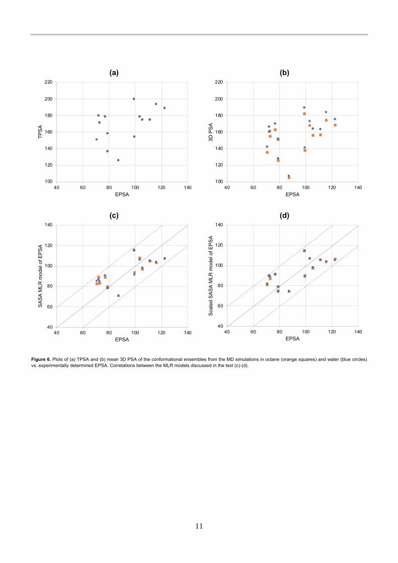
To correlate calculated PSA with experimental results, the chromatographic EPSA method was applied, [3, 4] see Table 2 for structural and experimental properties. This method was developed specifically to obtain a measure of surface polarity that could be used to predict permeability for e.g., cyclic peptides. For small, non-chameleonic molecules, the chromatographic retention time was linearly correlated with the calculated TPSA values for a set of 118 compounds with TPSA in the range of 40-130, and a very good correlation (R2 = 0.94) was found. [3] In figure 5, the chromatographically derived EPSA values are indicated as green bars. The PROTAC molecule was not included in the EPSA determination. The typical small molecule eliglustat (7) and the PPI inhibitor venetoclax (11) are the only molecules in the set for which the EPSA value is close to the TPSA and to the MD-derived mean PSA values. It is worth noting that venetoclax (11) is likely zwitterionic under the conditions of the EPSA determination, and this may be expected to lead to a much higher apparent polarity than would be expected from the PSA of the neutral, uncharged form. The molecular dynamics were carried out on the uncharged, neutral form rather than the zwitterionic form of 11. For all other molecules, the EPSA is lower than the PSA. There is essentially no correlation between EPSA and PSA or TPSA, see Figure 6a-b and Table 3. In light of the discussion above of the limitations of PSA as a measure of polarity, this is

not surprising: PSA (or TPSA) is not a good descriptor of surface polarity because it lumps together donor and acceptor areas and ignores the differences in hydrogen bonding strengths between different functional groups. It is also much less sensitive than SASA to conformational effects that shield polarity.

9

.

Table 2. Structural and experimental properties of the 24 drug molecules and one preclinical PROTAC studied in this work.[a]

Cpd Compound name MW TPSA HBA HBD Class log Doct log Dcyc log Dtol Dlog Doct-tol EPSA

1 Aliskiren 551.76 146.13 9 6 Base 1.1 -0.5 -0.4 1.5 88.7

2 Avanafil 483.95 125.39 10 3 Neutral 3.4 0.5 2.9 0.5 87.6

3 Dabigatran etexilate 627.73 151.53 12 3 Neutral 3.3 -0.6 3.5 -0.2 99.6

4 Atazanavir 704.85 171.22 13 5 Neutral 4.2 0.6 2.7 1.5 73.0

5 Cobicistat 776.03 138.02 12 3 Weak base 4.0 1.8 3.1 0.9 82.1

6 Edoxaban 548.06 136.63 11 3 Neutral 1.8 -2.2 0.7 1.1 79.1

7 Eliglustat 404.54 71.03 6 2 Base 2.2 0.4 1.7 0.5 76.5

8 Sofosbuvir 529.45 158.18 12 3 Neutral 1.6 <0 -0.6 2.2 79.1

9 Erythromycin 733.93 193.91 14 5 Base 1.4 -1.6 0.2 1.1 80.0

10 Tacrolimus 804.02 178.36 13 3 Neutral >4 1.6 [b] 77.3

11 Venetoclax 868.44 177.69 14 3 Zwitterion >4 [c] >3 162.2

12 Asunaprevir 748.29 182.33 14 3 Acid >3 1.0 3.4 94.7

13 Boceprevir 519.68 150.70 10 5 Neutral 3.8 -1.9 0.5 3.3 71.0

14 Telaprevir 679.85 179.56 13 4 Neutral 4.6 0.3 [c] 72.5

15 Glecaprevir 838.87 195.22 15 3 Acid 2.7 -0.5 2.4 0.3 112.3

16 Grazoprevir 766.91 195.22 15 3 Acid 2.7 0.2 2.9 -0.2 96.2

17 Paritaprevir 765.88 189.65 14 3 Acid 3.1 -0.5 3.0 0.1 135.5

18 Simeprevir 749.94 156.89 12 2 Acid >4 -0.5 >3 124.0

19 Daclatasvir 738.87 174.64 14 4 Neutral 4.0 -0.8 2.4 1.6 106.0

20 Ombitasvir 894.11 178.72 15 4 Neutral 4.3 1.6 >3 103.5

21 Pibrentasvir 1113.18 199.58 18 4 Neutral >4 -0.3 >3 99.3

22 Elbasvir 882.02 188.80 16 4 Neutral 4.4 2.2 [b] 122.8

23 Ledipasvir 889.00 174.64 14 4 Neutral >4 -0.5 [b] 111.5

24 Velpatasvir 883.00 193.10 16 4 Neutral 4.5 0.8 >3 116.1

25 PROTAC 1034.11 236.63 19 4 Neutral [b] [b] [b] [b]

[a] HBA and HBD, number of hydrogen bond acceptors and donors respectively according to Lipinski’s definition; [25] log Doct, log Dcyc and log Dtol, experimentally determined log D at pH 7.4 in water/1-octanol, water/cyclohexane and water/toluene respectively, see Experimental section for details. [b] Compound not available. [c] Not detectable.

To investigate if the scaled PSA concept would give a better model for polarity as measured using EPSA, MLR models were fitted to Equation 4. This is similar to Equation 3 above, but because a conformational ensemble rather than a single conformation must now be considered, the arithmetic mean values over the conformational ensembles were used for Stot, SHBA and SHBD. EPSA = ( + *!010+++++ + ,!!"#++++++ + -!!".++++++ (4)

To avoid complications due to charged species, only the neutral molecules were used (n = 14). The results are summarized in Table 3 and correlations are visualized in Figure 6, panels c and d. The best fits were obtained when using SASA and considering donors and acceptors separately, and very small differences between the solvents were observed. Interestingly, scaling the surface areas did not result in an improvement, unlike the results obtained for the Platts dataset discussed above. The mean

10

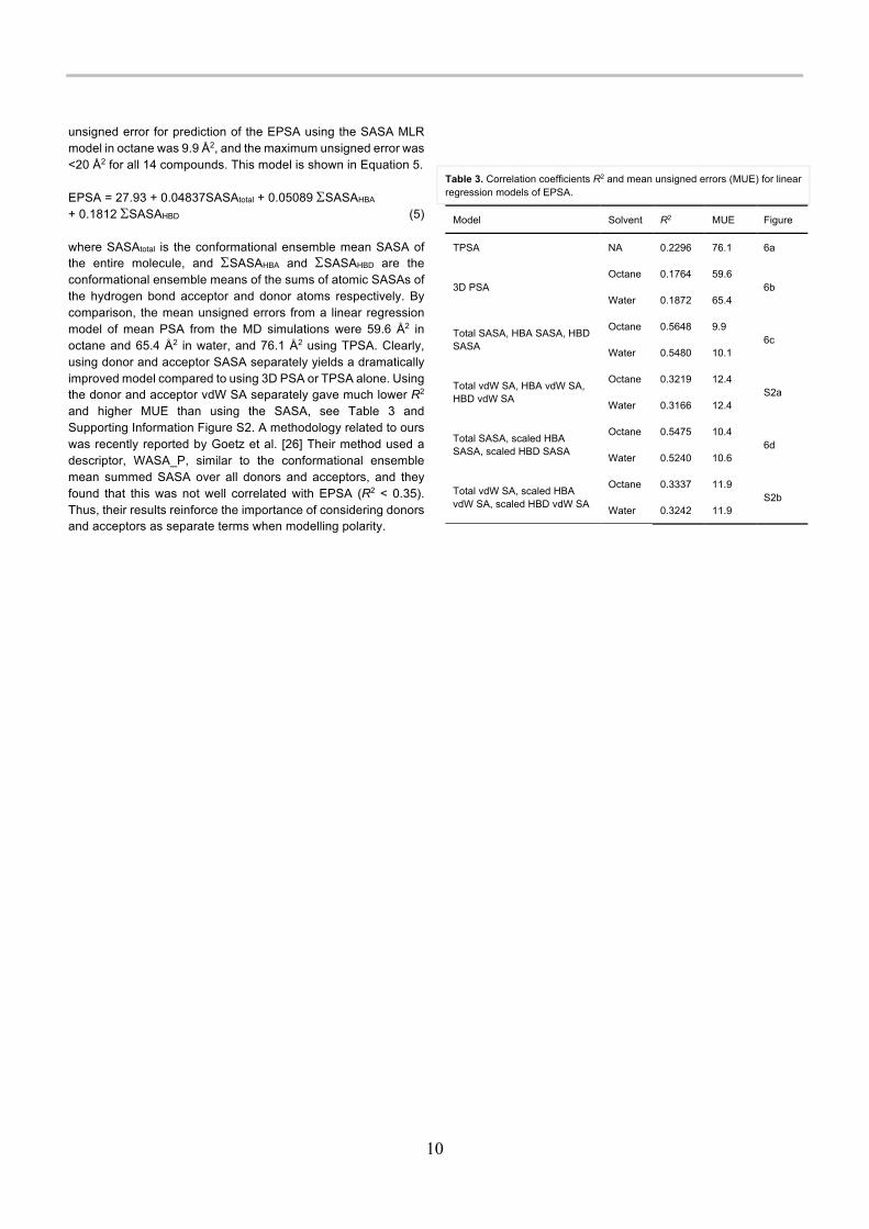
unsigned error for prediction of the EPSA using the SASA MLR model in octane was 9.9 Å2, and the maximum unsigned error was <20 Å2 for all 14 compounds. This model is shown in Equation 5. EPSA = 27.93 + 0.04837SASAtotal + 0.05089 SSASAHBA + 0.1812 SSASAHBD (5) where SASAtotal is the conformational ensemble mean SASA of the entire molecule, and SSASAHBA and SSASAHBD are the conformational ensemble means of the sums of atomic SASAs of the hydrogen bond acceptor and donor atoms respectively. By comparison, the mean unsigned errors from a linear regression model of mean PSA from the MD simulations were 59.6 Å2 in octane and 65.4 Å2 in water, and 76.1 Å2 using TPSA. Clearly, using donor and acceptor SASA separately yields a dramatically improved model compared to using 3D PSA or TPSA alone. Using the donor and acceptor vdW SA separately gave much lower R2 and higher MUE than using the SASA, see Table 3 and Supporting Information Figure S2. A methodology related to ours was recently reported by Goetz et al. [26] Their method used a descriptor, WASA_P, similar to the conformational ensemble mean summed SASA over all donors and acceptors, and they found that this was not well correlated with EPSA (R2 < 0.35). Thus, their results reinforce the importance of considering donors and acceptors as separate terms when modelling polarity.

Table 3. Correlation coefficients R2 and mean unsigned errors (MUE) for linear regression models of EPSA.

Model Solvent R2 MUE Figure

TPSA NA 0.2296 76.1 6a

3D PSA Octane 0.1764 59.6

6b Water 0.1872 65.4

Total SASA, HBA SASA, HBD SASA

Octane 0.5648 9.9 6c

Water 0.5480 10.1

Total vdW SA, HBA vdW SA, HBD vdW SA

Octane 0.3219 12.4 S2a

Water 0.3166 12.4

Total SASA, scaled HBA SASA, scaled HBD SASA

Octane 0.5475 10.4 6d

Water 0.5240 10.6

Total vdW SA, scaled HBA vdW SA, scaled HBD vdW SA

Octane 0.3337 11.9 S2b

Water 0.3242 11.9

11

Figure 6. Plots of (a) TPSA and (b) mean 3D PSA of the conformational ensembles from the MD simulations in octane (orange squares) and water (blue circles) vs. experimentally determined EPSA. Correlations between the MLR models discussed in the text (c)-(d).

100

120

140

160

180

200

220

40 60 80 100 120 140

TPSA

EPSA

(a)

100

120

140

160

180

200

220

40 60 80 100 120 140

3D P

SA

EPSA

(b)

40

60

80

100

120

140

40 60 80 100 120 140

Scal

ed S

ASA

MLR

mod

el o

f EPS

A

EPSA

(d)

40

60

80

100

120

140

40 60 80 100 120 140

SASA

MLR

mod

el o

f EPS

A

EPSA

(c)

12

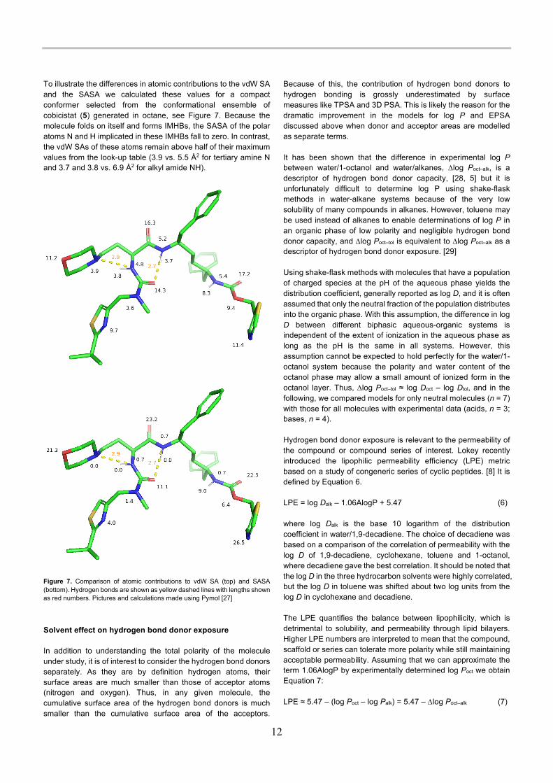
To illustrate the differences in atomic contributions to the vdW SA and the SASA we calculated these values for a compact conformer selected from the conformational ensemble of cobicistat (5) generated in octane, see Figure 7. Because the molecule folds on itself and forms IMHBs, the SASA of the polar atoms N and H implicated in these IMHBs fall to zero. In contrast, the vdW SAs of these atoms remain above half of their maximum values from the look-up table (3.9 vs. 5.5 Å2 for tertiary amine N and 3.7 and 3.8 vs. 6.9 Å2 for alkyl amide NH).

Figure 7. Comparison of atomic contributions to vdW SA (top) and SASA (bottom). Hydrogen bonds are shown as yellow dashed lines with lengths shown as red numbers. Pictures and calculations made using Pymol [27]

Solvent effect on hydrogen bond donor exposure In addition to understanding the total polarity of the molecule under study, it is of interest to consider the hydrogen bond donors separately. As they are by definition hydrogen atoms, their surface areas are much smaller than those of acceptor atoms (nitrogen and oxygen). Thus, in any given molecule, the cumulative surface area of the hydrogen bond donors is much smaller than the cumulative surface area of the acceptors.

Because of this, the contribution of hydrogen bond donors to hydrogen bonding is grossly underestimated by surface measures like TPSA and 3D PSA. This is likely the reason for the dramatic improvement in the models for log P and EPSA discussed above when donor and acceptor areas are modelled as separate terms. It has been shown that the difference in experimental log P between water/1-octanol and water/alkanes, Dlog Poct–alk, is a descriptor of hydrogen bond donor capacity, [28, 5] but it is unfortunately difficult to determine log P using shake-flask methods in water-alkane systems because of the very low solubility of many compounds in alkanes. However, toluene may be used instead of alkanes to enable determinations of log P in an organic phase of low polarity and negligible hydrogen bond donor capacity, and Dlog Poct–tol is equivalent to Dlog Poct–alk as a descriptor of hydrogen bond donor exposure. [29] Using shake-flask methods with molecules that have a population of charged species at the pH of the aqueous phase yields the distribution coefficient, generally reported as log D, and it is often assumed that only the neutral fraction of the population distributes into the organic phase. With this assumption, the difference in log D between different biphasic aqueous-organic systems is independent of the extent of ionization in the aqueous phase as long as the pH is the same in all systems. However, this assumption cannot be expected to hold perfectly for the water/1-octanol system because the polarity and water content of the octanol phase may allow a small amount of ionized form in the octanol layer. Thus, Dlog Poct–tol ≈ log Doct – log Dtol, and in the following, we compared models for only neutral molecules (n = 7) with those for all molecules with experimental data (acids, n = 3; bases, n = 4). Hydrogen bond donor exposure is relevant to the permeability of the compound or compound series of interest. Lokey recently introduced the lipophilic permeability efficiency (LPE) metric based on a study of congeneric series of cyclic peptides. [8] It is defined by Equation 6. LPE = log Dalk – 1.06AlogP + 5.47 (6) where log Dalk is the base 10 logarithm of the distribution coefficient in water/1,9-decadiene. The choice of decadiene was based on a comparison of the correlation of permeability with the log D of 1,9-decadiene, cyclohexane, toluene and 1-octanol, where decadiene gave the best correlation. It should be noted that the log D in the three hydrocarbon solvents were highly correlated, but the log D in toluene was shifted about two log units from the log D in cyclohexane and decadiene. The LPE quantifies the balance between lipophilicity, which is detrimental to solubility, and permeability through lipid bilayers. Higher LPE numbers are interpreted to mean that the compound, scaffold or series can tolerate more polarity while still maintaining acceptable permeability. Assuming that we can approximate the term 1.06AlogP by experimentally determined log Poct we obtain Equation 7: LPE ≈ 5.47 – (log Poct – log Palk) = 5.47 – Dlog Poct–alk (7)

13

Thus, minimizing Dlog Poct–alk (or equivalently Dlog Poct–tol) will maximize lipophilic permeability efficiency. Methods that would allow the prediction of Dlog Poct–tol ahead of synthesis would be valuable to chemists faced with the design of large molecules with acceptable permeability and solubility. To determine if the MD protocol and scaled surface area concepts introduced here would yield such a predictive model, we investigated the correlations between Dlog Poct–tol and various representations of exposed hydrogen bond donor potential. In the present study, we attempted to determine log D in water/toluene and water/cyclohexane systems using shake-flask methods. Determinations were in many cases difficult due to low or no observed signals in the MS detection of analytes. This is likely due to poor solubility for several compounds. Because the water/toluene system yielded higher quality data than the water/cyclohexane system, we based our modelling on the former. To investigate the extent of intramolecular hydrogen bonding in the conformational ensembles generated by our MD protocol, each conformer was analysed using the Schrödinger Maestro [20] default settings for hydrogen bond detection and the number of IMHBs was recorded. The distributions of IMHB counts in water and octane are shown in Figure 8a. Most of the molecules studied show no or one single IMHB in water, and more IMHBs in octane. The exposed hydrogen bond donor count of each conformer was then calculated as the number of donors not involved in IMHB formation by subtracting the number of IMHBs from the total number of donors. The distributions of exposed hydrogen bond donor counts are shown in Figure 8b. To investigate if Dlog Poct–tol is correlated with various hydrogen bond donor surface representations, or with counts of solvent-exposed donors or total Lipinski donor counts, correlation coefficients for linear regression models were calculated, see Table 4. By far the best correlation with experimental Dlog Poct–tol was found for the mean scaled hydrogen bond donor SASA from the octane MD simulations, see Figure 9. Importantly, both neutral, acidic and basic molecules were included, and only a slight improvement in the correlation was observed when only neutral molecules were considered. Thus, the mean scaled SASA derived from MD simulations in octane is an excellent predictor of Dlog Poct–tol, and it can be applied to both neutral and charged molecules. Plots of Dlog Poct–tol vs. the other hydrogen bond donor representations in Table 4 are shown in the Supporting Information Figures S3 (octane simulations) and S4 (water simulations).

Table 4. Correlation coefficients R2 for linear regression models of Dlog Poct–tol.

HBD representation All compounds Neutral compounds

Octane Water Octane Water

Mean HBD vdW SA 0.4344 0.3980 0.4600 0.4469

Mean HBD SASA 0.4529 0.4762 0.2570 0.3789

Mean scaled HBD vdW SA 0.4428 0.4222 0.4824 0.4842

Mean scaled HBD SASA 0.8277 0.7474 0.9166 0.8548

Mean solvent-exposed HBD count

0.4063 0.4174 0.6597 0.5003

Lipinski HBD count 0.3369 0.3878

The distributions of scaled hydrogen bond donor SASA for each of the molecules in the two solvents are shown as split violin plots in Figure 8c. Many of the molecules show differences in hydrogen bond donor exposure, and the magnitude of the differences can be considered a quantitative measure of chameleonicity.

14

Figure 8. Distributions of (a) counts of IMHBs, (b) exposed hydrogen bonds, and (c) scaled HBD SASA for the conformational ensembles in octane (orange) and water (blue). Histogram representations are shown in panels (a) and (b), and violin plot representations in panel (c). Horizontal bars in panel (c) indicate the mean of the distributions. The chameleonic efficiency indices are given as labels on beige background. The CHE index is shown in panels (a) and (b), and the CDE index is shown in panel (c).

15

Figure 9. Correlation between scaled HBD SASA from the octane MD simulations and experimental Dlog Poct–tol. The mean values of scaled HBD SASA are shown as filled circles and the full distributions over the conformational ensembles as violin plots. Linear regressions using the means are shown for all compounds (solid, grey line), and for only neutral compounds (dashed, orange line), with the corresponding equations and correlation coefficients listed in the legend.

Chameleonicity quantified: Chameleonic efficiency indices The models of EPSA and Dlog Poct–tol presented above are primarily relevant for the understanding of membrane permeability. The best models were derived from the conformational ensembles in octane, where IMHB formation shields polarity. However, to achieve sufficient aqueous solubility, hydrogen bonds to water must be possible. The extent to which a molecule is able to change from IMHB formation in octane to intermolecular hydrogen bonding with water is the essence of chameleonicity. To enable the prospective evaluation of molecular designs ahead of synthesis, we propose two quantitative measures of chameleonicity: The chameleonic efficiency indices. The numerical values of the indices defined below are shown in Figure 8 as labels on a beige background. The chameleonic intramolecular hydrogen bonding efficiency (CHE) quantifies the difference in IMHB counts between non-polar and aqueous environments, and is defined by Equation 8: CHE = (IMHBoct – IMHBwat)/HBDLipinski (8) where IMHBoct and IMHBwat are the conformational ensemble mean number of IMHBs formed in octane and water respectively, and HBDLipinski is the number of hydrogen bond donors according to Lipinski’s definition. [25] This index may be useful to evaluate how successful various molecular designs are at forming IMHBs in non-polar environments while exposing all hydrogen bond donors in water. It has the property that it is 1 only when all donors are engaged in IMHBs in octane and no IMHBs are formed in water. This is the best case possible but is unlikely to be achieved in practice. The compound with the highest CHE in this study, the macrocyclic HCV NS3/4A inhibitor glecaprevir (15), reaches a

value of 0.52, with another three HCV NS3/4A and NS5A inhibitors (12, 21, and 24) in the range of 0.40-0.42. When there is no difference in IMHB formation between the solvents, the index is 0, corresponding to a non-chameleonic molecule. Although a clear cut-off between chameleonic and non-chameleonic molecules is not possible to determine based on the present results, values in the range of 0.3 to 0.5 should be considered as good design targets. The chameleonic hydrogen bond donor efficiency (CDE) quantifies the difference in hydrogen bond donor potential between non-polar and aqueous environments expressed as the scaled hydrogen bond donor SASA. It is defined by Equation 9: CDE = 1 – (SASAHBD,oct/SASAHBD,wat) (9) where SASAHBD,oct and SASAHBD,wat are the conformational ensemble means in octane and water respectively of the scaled donor SASA (Equation 2). This index may be useful to evaluate the difference in hydrogen bond donor potential between non-polar environments and water. It has the property that it is 1 when there is no hydrogen bond donor exposure in octane (best case), and 0 when there is no difference in exposed donor potential between octane and water. The compound with the highest CDE is the PROTAC (25) with a CDE = 0.76 and a CHE = 0.31. Because the two indices quantify different aspects of chameleonicity, they are not well correlated. We propose that they are both useful to triage molecular designs but for slightly different purposes. The CHE index is useful to test if intended IMHBs are formed in non-polar environments but not in water, while the CDE index is useful to evaluate the consequences of IMHB formation for the exposed hydrogen bond donor potential. Limitations of MD simulations The method presented herein is based on plain MD simulations at a constant temperature of 300 K and a constant pressure of 1 bar with a cumulative simulation time of 250 ns. Thus, to thoroughly sample the conformational space of the molecule under study, every rotatable bond must be able to rotate sufficiently fast that multiple rotamers will appear within the 250 ns time window. In other words, the half-life for bond rotation, t1/2 = (ln 2)/k where k is the rate of rotation, must be considerably less than 250 ns. Using the Eyring equation (10) and assuming a transmission factor κ = 1, this is equivalent to a rotational barrier ΔG‡ = 8.7 kcal/mol at a temperature T = 300 K.

. = 0 ."1ℎ 3245‡67

(10) where κ is the transmission coefficient, kB is Boltzmann's constant, h is Planck's constant, and R is the gas constant. For most single bonds, the rotational barrier will be much lower than this value, but if constraints like cyclisation or partial double bond character are present, the rotational barriers can easily surpass this value. A typical amide bond has a rotational barrier of 15-20 kcal/mol corresponding to a half-life of 10-40 ms. It is thus extremely unlikely to observe a single rotational event for an amide bond using plain MD simulations of the time scales used here. Because

16

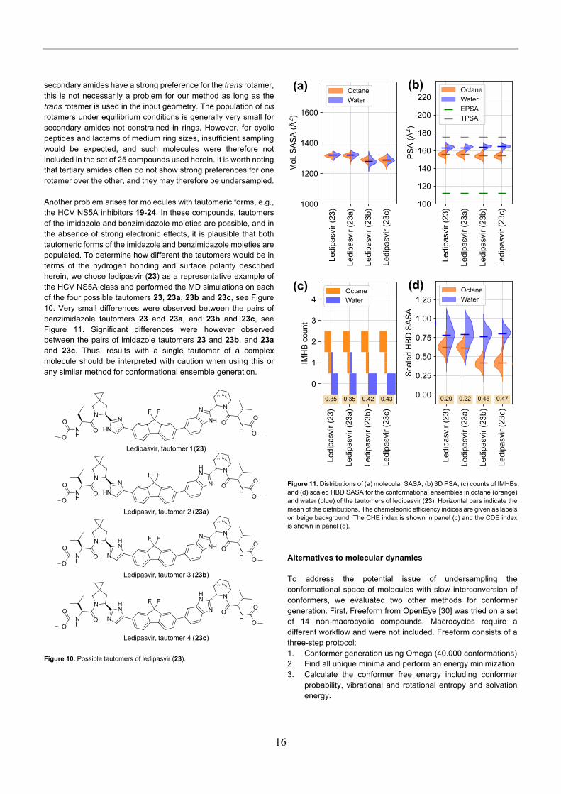
secondary amides have a strong preference for the trans rotamer, this is not necessarily a problem for our method as long as the trans rotamer is used in the input geometry. The population of cis rotamers under equilibrium conditions is generally very small for secondary amides not constrained in rings. However, for cyclic peptides and lactams of medium ring sizes, insufficient sampling would be expected, and such molecules were therefore not included in the set of 25 compounds used herein. It is worth noting that tertiary amides often do not show strong preferences for one rotamer over the other, and they may therefore be undersampled. Another problem arises for molecules with tautomeric forms, e.g., the HCV NS5A inhibitors 19-24. In these compounds, tautomers of the imidazole and benzimidazole moieties are possible, and in the absence of strong electronic effects, it is plausible that both tautomeric forms of the imidazole and benzimidazole moieties are populated. To determine how different the tautomers would be in terms of the hydrogen bonding and surface polarity described herein, we chose ledipasvir (23) as a representative example of the HCV NS5A class and performed the MD simulations on each of the four possible tautomers 23, 23a, 23b and 23c, see Figure 10. Very small differences were observed between the pairs of benzimidazole tautomers 23 and 23a, and 23b and 23c, see Figure 11. Significant differences were however observed between the pairs of imidazole tautomers 23 and 23b, and 23a and 23c. Thus, results with a single tautomer of a complex molecule should be interpreted with caution when using this or any similar method for conformational ensemble generation.

Figure 10. Possible tautomers of ledipasvir (23).

Figure 11. Distributions of (a) molecular SASA, (b) 3D PSA, (c) counts of IMHBs, and (d) scaled HBD SASA for the conformational ensembles in octane (orange) and water (blue) of the tautomers of ledipasvir (23). Horizontal bars indicate the mean of the distributions. The chameleonic efficiency indices are given as labels on beige background. The CHE index is shown in panel (c) and the CDE index is shown in panel (d).

Alternatives to molecular dynamics To address the potential issue of undersampling the conformational space of molecules with slow interconversion of conformers, we evaluated two other methods for conformer generation. First, Freeform from OpenEye [30] was tried on a set of 14 non-macrocyclic compounds. Macrocycles require a different workflow and were not included. Freeform consists of a three-step protocol: 1. Conformer generation using Omega (40.000 conformations) 2. Find all unique minima and perform an energy minimization 3. Calculate the conformer free energy including conformer

probability, vibrational and rotational entropy and solvation energy.

17

The conformational ensembles generated by Freeform were similar to those generated by MD in terms of total molecular and polar surface areas, scaled hydrogen bond donor SASA, and IMHB counts, see Supporting Information Figure S5. The correlation between scaled hydrogen bond donor SASA and Dlog Poct–tol was similar to that obtained for MD, See Supporting Information Figure S6. Freeform in vacuum gave a correlation coefficient R2 = 0.91-0.93 depending on the energy window (1-5 kcal/mol) used to select conformers. Second, we selected one example, glecaprevir (15) to test with Prime MCS from Schrödinger. [20, 31] Prime MCS does not allow changing the dielectric as it performs the final energy minimization in vacuum, so the generated conformers would need to be re-evaluated in water to get accurate conformational energies in that solvent. Thus, the results are more comparable to those of MD in octane than in water. Prime MCS consists of a three-step protocol: 1. Sampling splits naked macrocycle backbone into two pieces

sampled independently using a library of known angles. 2. Both pieces are then reconnected if they match. 3. The side chains are built back to the macrocycle and the

structure is energy minimized. The conformational ensemble generated by Freeform for glecaprevir (15) was very similar to that generated by MD in octane in terms of polar surface areas and hydrogen bond donor SASA, see supporting information Figure S7. Compared to MD, the total molecular SASA distribution was wider with a lower mean, and slightly fewer intramolecular hydrogen bonds were present on average. These two alternative methods sample the conformational space well, but do not explicitly take solvent molecules into account. Thus, the conformers they generate may not correctly represent intermolecular hydrogen bonding with solvent molecules.

Conclusion

The generation of conformational ensembles in aqueous and non-polar environments using molecular dynamics yielded valuable insights into the chameleonic properties of the set of compounds in Figure 1. The concept of scaling the surface areas of hydrogen bond donors and acceptors with their respective hydrogen bonding strengths was updated and confirmed to improve the prediction of log P in cyclohexane/water as previously reported. [14] Predictive models for EPSA and Dlog Poct–tol were derived from the conformational ensembles obtained from MD simulations in octane. The best model for EPSA (R2 = 0.56, MUE = 9.9 Å2) was obtained when the hydrogen bond acceptor and donor SASA were treated as separate terms, with the total molecular SASA as a third term (Equation 5). Unlike the case of the log P prediction, no improvement in the EPSA model was found when using scaled surface areas. An excellent correlation was found between experimentally determined Dlog Poct–tol and the octane MD conformational ensemble mean hydrogen bond donor SASA scaled with Abraham’s A hydrogen bond strength (Figure 9). The ability to predict EPSA and Dlog Poct–tol is expected to be helpful to optimize membrane permeability but does not address the balance between permeability and solubility. This balance is impacted by the degree of chameleonicity of the molecule. To

quantify this property, two indices of chameleonic efficiency, the chameleonic intramolecular hydrogen bonding efficiency (CHE) and the chameleonic hydrogen bond donor efficiency (CDE), are proposed. Taken together, these models and efficiency indices are envisaged to be valuable tools for the design of chameleonic molecules with an acceptable balance of permeability and solubility.

Experimental Section

Materials

Compounds 1-24 were sourced via Aldrich Market Select using the following suppliers: Adooq Bioscience (California, USA) – boceprevir (13), dabigatran etexilate (3), daclatasvir (19), eliglustat (7), ledipasvir (23), tacrolimus (10), telaprevir (14); Aldrich-CPR (Sigma-Aldrich, Wisconsin, USA) – erythromycin (9); Ambeed Inc (Illinois, USA) – aliskiren (1), atazanavir (4), sofosbuvir (8), venetoclax (11); Carbosynth Ltd (Oxfordshire, UK) – pibrentasvir (21); Cayman Chemical – simeprevir (18), velpatasvir (24); MedChem Express (New Jersey, USA) – avanafil (2), cobicistat (5), elbasvir (22), glecaprevir (15), ombitasvir (20); Target Molecule Corp. (Massachusetts, USA) – asunaprevir (12), edoxaban (6), grazoprevir (16), paritaprevir (17). Stock solutions in DMSO with a concentration of 10 mM were prepared and used for all analyses. Ammonium formate, DMSO, formic acid, methanol, Na2HPO4 and KH2PO4 were sourced from Thermo Fisher Scientific (Leicestershire, UK). Ammonium acetate, cyclohexane, metoprolol, octanol and toluene were sourced from Merck/Sigma-Aldrich (Dorset, UK). 0.1 M phosphate buffer (pH7.4) was prepared by combining aqueous solutions of 0.05 M Na2HPO4 and 0.05 M KH2PO4. For log D measurements, Abgene 96-well 0.8 mL polypropylene plates (Thermo Fisher Scientific, Leicestershire, UK) were used; and Corning Costar 1.2 mL polypropylene cluster tubes (Merck/Sigma-Aldrich, Dorset, UK) were used as sample tubes. UPLC analysis for log D measurements used a Acquity HSS T3 (1.8 µm) 2.1 x 30 mm (Waters, Hertfordshire, UK) column fitted with SecurityGuard ULTRA fully porous polar C18 cartridge (Phenomenex, Cheshire, UK). EPSA analysis used a 20 mM ammonium formate in methanol mobile phase modifier, CO2 (2.8 grade, 99.8% purity) from Air Products (Oxfordshire, UK) and a 4.6 mm × 250 mm Chirex 3014 column with a 5 μm particle and 100 Å pore size (Phenomenex, Cheshire, UK).

Instrumentation and analysis

All log D measurements used a FB15051 Fisherbrand sonicator (Thermo Fisher Scientific, Leicestershire, UK), Heraeus Multifuge X3R centrifuge (Thermo Fisher Scientific, Leicestershire, UK) and Eppendorf Thermomixer comfort (Eppendorf, Hertfordshire, UK); and analysis was performed via ultra-high pressure liquid chromatography (UPLC) incorporating mass spectrometer (MS) detection. The UPLC-MS system was controlled via MassLynx software (Waters, Hertfordshire, UK) and consisted of an Acquity binary solvent manager (Waters, Hertfordshire, UK), Acquity four-position heated column manager (Waters, Hertfordshire, UK), 2777 ultra-high pressure autosampler (Waters, Hertfordshire, UK) and a Xevo triple quadrupole MS (Waters, Hertfordshire, UK). The column was heated to 40 °C and an injection volume of 4 µL was used for all samples analysed. The gradient ranged from 100% mobile phase A and 0% methanol to 5% mobile phase A and 95% methanol at a flow rate of 1000 µL min-1 over 0.9 min. For the majority of compounds, the mobile phase A was 10 mM ammonium formate plus 0.1% v/v formic acid in water; for asunaprevir (12), glecaprevir (15), grazoprevir (16) and simeprevir (18) mobile phase A was 10 mM ammonium acetate in water. The MS analysis was carried out in multiple reaction monitoring (MRM) mode using MRM methods developed for each compound. TargetLynx software (Waters, Hertfordshire, UK) was used to determine a compound’s peak area response ratio to the internal standard for all MRM chromatograms associated to all serial diluted organic and buffer phase samples. A relative

18

concentration calibration curve was established using the peak area response ratios of at least three of the serial diluted samples from either the organic or buffer phase.

EPSA analysis was performed following the reported method [4] via supercritical fluid chromatography (SFC) using a Waters-Thar Resolution MS SFC system, incorporating a Waters 3100 single quadrupole with an ESI source (Hertfordshire, UK), and controlled via MassLynx software (Waters, Hertfordshire, UK). The column was heated to 40 °C and an injection volume of 10 µL was used for all samples analysed. A flow rate of 5 mL min-1 and an outlet backpressure of 140 bar was used. A sample run lasted 17 min, during which time the mobile phase composition was varied, using a linear gradient, from 5% to 60% modifier at 5% min-1, holding at 60% for 5 min before returning to 5%. The MS scanning mode used a mass range of 150-1500 m/z.

Experimental procedure for log D measurements

An aliquot (10 µL) of a 10 mM DMSO stock of a compound was added to a well within a 96-well plate containing organic solvent (490 µL; 1-octanol, cyclohexane or toluene), pre-saturated with 0.1 M phosphate buffer (pH 7.4). The 96-well plate was then sonicated (0.50 hr) and subsequently centrifuged (200 g, 22 °C, 0.25 hr) to pellet any undissolved compound. An aliquot (300 µL) of the organic phase solution was added to an individual sample tube containing 0.1 M phosphate buffer (600 µL, pH 7.4), pre-saturated with organic solvent, which was allowed to equilibrate on a thermomixer (1000 rpm, 37⁰C, 0.50 hr) and subsequently centrifuged (200 g, 22 °C, 5 min). An aliquot (100 µL) of the partition mixture organic phase was transferred to another sample tube; the remaining organic phase was removed. An aliquot (100 µL) of the partition mixture buffer phase was transferred to another sample tube and subsequently centrifuged (200 g, 22 °C, 5 min). An aliquot (5 µL) of the isolated partition mixture organic phase was dissolved in DMSO (95 µL) and mixed; and a further four serial 10-fold dilutions in DMSO were made (i.e., 5 µL of diluted solution in 45 µL DMSO). An aliquot (5 µL) of the isolated partition mixture buffer phase was dissolved in DMSO (95 µL) and mixed; and a further two serial 10-fold dilutions in DMSO were made (i.e., 5 µL of diluted solution in 45 µL DMSO). Each diluted sample was further diluted 10-fold into DMSO containing metoprolol (0.55 µM), as an internal standard, and subsequently analysed via UPLC-MSMS. A log D value for a compound was determined from the logarithmic base-10 of the ratio of its relative concentration in the organic phase compared to its relative concentration in the buffer phase; adjusted for dilution factors.

Experimental procedure for EPSA measurements

An aliquot (15 µL) of a 10 mM DMSO stock of a compound was diluted to 3 mM using DMSO (35 µL). The subsequent sample was analysed on the SFC-MS system in triplicate.

Molecular dynamics simulations

Molecular dynamics simulations were performed using Desmond v5.1 from the Schrödinger suite 2017-3 with default parameters as reported previously. [9] For each molecule in Figure 1, five runs of 50 ns saving a frame every 0.1 ns were performed for each solvent. Thus, a total of 2500 conformations for each drug-solvent combination was obtained. The neutral form of the molecule was used in all cases. A cubic simulation box with a buffer size of 20 Å was used to prevent the ligand to interact with its own image. For simulations in water the TIP3P model was used and for simulations in n-octane a custom solvent box was constructed as recommended by Schrödinger. All simulations were performed using the OPLS3 force field. Per-atom exposed vdW SA and SASA were calculated for each conformer using the Schrödinger Maestro [20] API function ‘calculate_sasa’ from the ‘schrodinger.structutils.analyze’ library with a probe radius of 0.000001 for vdW SA and 1.4 for SASA. Intramolecular hydrogen bonds were detected and counted using the API function ‘get_hydrogen_bonds’ from the ‘schrodinger.structutils.interactions.hbond’

library with default parameters. To derive the fraction exposed surface area, the exposed surface area of each polar atom was divided by the maximum possible exposed surface area for an atom of the same type in a molecule where no steric shielding is possible. As an example, the maximum exposed surface area of an alkanol oxygen atom was defined as the surface area of the oxygen atom in methanol. For each atom type, a prototypical molecule was used to construct table entries for maximum exposed vdW SA and SASA, see Supporting Information Tables S1 and S2. The Schrödinger API was used as described above for these calculations. Hydrogen bond strengths were added to the tables from the literature, [15, 16, 17, 21] and the values of Abraham’s A and pKBHX used for each atom are shown in Supporting Information Table S3. All calculations were performed using a Python script within the Maestro interactive Python console, see Supporting Information.

Acknowledgements

The authors express their gratitude to Andrew Halliwell (Cyprotex, UK), Katy Barnes (Cyprotex, UK) and Alexander Scott (Cyprotex, UK) for performing the log D measurements, and to Richard Marston (Evotec, UK) for performing the EPSA measurements.

Keywords: chameleonic properties • polar surface area • hydrogen bonding • molecular dynamics

[1] B. C. Doak, B. Over, F. Giordanetto, J. Kihlberg, Chem. Biol. 2014, 21, 1115-1142.

[2] A. Whitty, M. Zhong, L. Viarengo, D. Beglov, D. R. Hall, S. Vajda, Drug Discov. Today 2016, 21, 712-717.

[3] G. H. Goetz, W. Farrell, M. Shalaeva, S. Sciabola, D. Anderson, J. Yan, L. Philippe, M. J. Shapiro, J. Med. Chem. 2014, 57, 2920-2929.

[4] G. H. Goetz, L. Philippe, M. J. Shapiro, ACS Med. Chem. Lett. 2014, 5, 1167-1172.

[5] N. El Tayar, R.-S. Tsai, B. Testa, P.-A. Carrupt, A. Leo, J. Pharm. Sci. 1991, 80, 590-598.

[6] G. Caron, G. Ermondi, Mini-Rev. Med. Chem. 2003, 3, 821-830. [7] G. Caron, M. Vallaro, G. Ermondi, Med. Chem. Commun. 2017, 8, 1143-

1151. [8] M. R. Naylor, A. M. Ly, M. J. Handford, D. P. Ramos, C. R. Pye, A.

Furukawa, V. G. Klein, R. P. Noland, Q. Edmondson, A. C. Turmon, W. M. Hewitt, J. Schwochert, C. E. Townsend and C. N. Kelly, M.-J. Blanco, R. S. Lokey, J. Med. Chem. 2018, 61, 11169-11182.

[9] A. Ritzén, L. David in Successful Drug Discovery, Volume 4 (Eds.: J. Fischer, C. Klein, W. E. Childers), Wiley-VCH, Weinheim, 2019, pp. 35-53.

[10] C. R. W. Guimarães, A. M. Mathiowetz, M. Shalaeva, G. Goetz, S. Liras, J. Chem. Inf. Model. 2012, 52, 882-890.

[11] C. J. Dickson, V. Hornak, R. A. Pearlstein, J. S. Duca, J. Am. Chem. Soc. 2017, 139, 442-452.

[12] P. Ertl, B. Rohde, P. Selzer, J. Med. Chem., 2000, 43, 3714-3717. [13] G. Caron, G. Ermondi, Future Med. Chem. 2016, 8, 2013-2016. [14] R. A. Saunders, J. A. Platts, New J. Chem. 2004, 28, 166-172. [15] M. H. Abraham, Chem. Soc. Rev. 1993, 22, 73-83. [16] M. H. Abraham, A. Ibrahim, A. M. Zissimos, J. Chromatogr. A 2004, 1037,

29-47. [17] C. Laurence, K. A. Brameld, J. Graton, J.-Y. Le Questel, E. Renault, J.

Med. Chem. 2009, 52, 4073-4086. [18] A. J. Green, P. L. A. Popelier, J. Chem. Inf. Model. 2014, 54, 553-561. [19] A. Leo, C. Hansch, D. Elkins, Chem. Rev. 1971, 71, 525-616. [20] Schrödinger Release 2020-3: Maestro, Schrödinger, LLC, New York, NY,

2020. [21] J. A. H. Schwöbel, R.-U. Ebert, R. Kühne, G. Schüürmann, J. Phys. Org.

Chem. 2011, 24, 1072-1080. [22] C. A. Bauer, G. Schneider, A. H. Göller, J. Cheminform. 2019, 11, 59. [23] E. Danelius, V. Poongavanam, S. Peintner, L. H. E. Wieske, M. Erdélyi,

J. Kihlberg, Chem. Eur. J. 2020, 26, 5231-5244.

19

[24] Y. Atilaw, V. Poongavanam, C. S. Nilsson, D. Nguyen, A. Giese, D. Meibom, M. Erdélyi, J. Kihlberg, ACS Med. Chem. Lett. 2021, 12, 107-114.

[25] C. A. Lipinski, F. Lombardo, B. W. Dominy, P. J. Feeney, Adv. Drug Delivery Rev. 2001, 46, 3-26.

[26] G. Russo, F. Barbato, L. Grumetto, L. Philippe, F. Lynen, G. H. Goetz, Int. J. Pharm. 2019, 560, 294-305.

[27] The PyMOL Molecular Graphics System, Version 2.0 Schrödinger, LLC. [28] X. Liu, B. Testa, A. Fahr, Pharm. Res. 2011, 28, 962-977. [29] M. Shalaeva, G. Caron, Y. A. Abramov, T. N. O’Connell, M. S. Plummer,

G. Yalamanchi, K. A. Farley, G. H. Goetz, L. Philippe, M. J. Shapiro, J. Med. Chem. 2013, 56, 4870-4879.

[30] SZYBKI/Freeform: OpenEye Scientific Software, Santa Fe, NM. [31] D. Sindhikara, S. A. Spronk, T. Day, K. Borrelli, D. L. Cheney, S. L. Posy,

J. Chem. Inf. Model. 2017, 57, 1881-1894.