Prediction and Prolongation of the Service Life

of Weathering Steel Highway Structures

by

Neal R. Damgaard

A thesis

presented to the University of Waterloo

in fulfillment of the

thesis requirement for the degree of

Master of Applied Science

in

Civil Engineering

Waterloo, Ontario, Canada, 2009

©Neal R. Damgaard 2009

ii

I hereby declare that I am the sole author of this thesis. This is a true copy of the thesis, including

any required final revisions, as accepted by my examiners. I understand that my thesis may be

made electronically available to the public.

iii

Abstract

Weathering steel is a high-strength, low-alloy steel which has been proven to provide a

significantly higher corrosion resistance than regular carbon steel. This corrosion

resistance is a product of the small amounts of alloying elements added to the steel,

which enable it to form a protective oxide layer when exposed to the environment. The

main advantage of its use in bridges is that, under normal conditions, it may be left

unpainted, leading to significantly reduced maintenance and environmental costs.

Weathering steel has been a material of choice for highway structures for almost half a

century, and a very large number of structures have been constructed with it. Although its

use has for the most part been successful, it has also become evident that, in

circumstances where there is the presence of salt and sulphur oxides, its performance is

deficient. In these situations the corrosion penetration rate is much higher than expected,

and the oxide layer forms in thick layers. This presents an added risk, since these layers

flake off and fall onto the roadway. The degree of corrosion on structures can be very

different, even if the structural type, location, and climate are similar.

Therefore the focus of the thesis is on the lifespan of weathering steel highway structures.

Primarily this research is concerned with the effect of corrosion on the integrity of these

structures, as well as ways of quantifying corrosion loss and protecting the structure from

further corrosion.

In order to determine the lifespan of weathering steel highway structures subject to

different rates of corrosion, a probabilistic structural analysis program has been

developed to assess the time-dependent reliability of the structure. This program used

iterative Monte Carlo simulation and a series of statistical variables relating to the

material, loading, and corrosion properties of the structure. A corrosion penetration

equation is used to estimate thickness loss at a selected interval, and the structural

properties of the bridge are modified accordingly. The ultimate limit states of shear,

moment, and bearing, and the fatigue limit state of web breathing, are taken into account.

Three types of structures are examined: simply-supported box and I-girder composite

bridges, and a two-span box girder bridge.

iv

Based on the structural analysis of the corroding bridge structures presented herein, it can

be seen that corrosion to the weathering steel girders can cause reduced service lives of

the structures. I-girder bridges are shown to be more susceptible to corrosion than box

girder bridges, with continuous box girder bridges showing the best performance. The

amount of truck traffic does not affect the reliability of the bridge. The short-span and

high strength steel bridges are more susceptible to corrosion loss, primarily because their

girders have thinner sections. A two-lane bridge also has better performance than the

wider bridges because the weight of the barriers and sidewalks is carried by fewer

girders, so these girders are stockier. The web breathing limit state is less significant than

the combined ultimate limit states. Lastly, and most importantly, inspection data from a

highway bridge is used to demonstrate the benefit that can be derived from using field

data to update the time-dependent reliability.

The ultrasonic thickness gauge (UTG) is a common tool for thickness measurement of

steel sections. When used to measure weathering steel, this instrument provides accurate

data about the depth of corrosion pits, but not their lateral dimensions. The measurement

does not include the corrosion layer on the opposite side of the plate from the one being

measured; however, if the corrosion layer is on the measured face, a disproportionate

increase in the measured thickness can be seen.

In order to prevent or minimize corrosion loss, the steel is currently painted, a process

with several environmental and financial disadvantages. Therefore, three novel protection

methods have been assessed in a cyclic corrosion test: a zinc metallizing, an aluminum-

zinc-indium alloy metallizing, and a zinc tape with a PVC topcoat. All these coatings are

designed to act not just as barriers, but also as sacrificial anodes. The test was run for 212

24-hr cycles, over the course of which the all the coatings were proven effective at

protecting the steel substrate, regardless of steel type and surface roughness and

pretreatment.

In conclusion, the threat to all types of weathering steel highway structures by

contaminant-induced corrosion is significant, but inspection data permits a more accurate

prediction of time-dependent reliability for a structure, and protective coatings are a

promising method of slowing the advance of corrosion.

v

Acknowledgements

I would like to thank the following persons for their varied contributions to this work:

• God. Also my wife, Maria, and my son, Paul, and all of my family.

• Dr. Scott Walbridge and Dr. Carolyn Hansson, invaluable co-supervisors of this

thesis, as well as Jamie Yeung, who did excellent work for this project, and of

whom great things are expected.

• Frank Pianca of the Ministry of Transportation of Ontario, Dave Whitmore and

the other excellent people of Vector Corrosion Technologies, and Florent

Lefevre-Schlick and his helpful coworkers at Essar Steel Algoma.

• For their technical support: Graham Cranston, Jovan Vukotic, Richard Morrison,

Mike Cocker, Randy Fagan, Dr. Shahzma Jaffer, Ken Su, Jim Merli, Dr. Giovanni

Cascante, John Boldt, Dr. Enming Hu, Mark Sobon, Ken Bowman, and others too

numerous to mention.

• For their friendship: Nathan, Allan, Carol, Matt and Deborah, Dave, Jon and

Maureen, Jessica, Liam, Ivan, Simon, Pete, Paul, all the members of the Civilators

FC, and everyone else who over the last couple of years has made doing a

master’s degree enjoyable, or at the very least memorable.

vi

Dedicated to my father

vii

TABLE OF CONTENTS

List of Figures ..................................................................................................................... x List of Tables .................................................................................................................... xv Chapter 1: Introduction ....................................................................................................... 1

1.1 Background .......................................................................................................... 1 1.2 Objectives............................................................................................................. 3 1.3 Scope .................................................................................................................... 3 1.4 Thesis Organization.............................................................................................. 4

Chapter 2: Literature Review.............................................................................................. 5 2.1 Corrosion of Weathering Steel............................................................................. 5

2.1.1 Corrosion Products........................................................................................ 5 2.1.2 Corrosion Reaction for Steel......................................................................... 5 2.1.3 Effect of Alloying Elements ......................................................................... 6 2.1.4 Effect of Road Salt on Weathering Steel ...................................................... 7 2.1.5 Corrosion Rate Equations ............................................................................. 7

2.2 Sacrificial Anode Protection of Weathering Steel ............................................. 10 2.2.1 Metallizing .................................................................................................. 10 2.2.2 Galvanic (Zinc) Tape .................................................................................. 11

2.3 Evaluating Corrosion Penetration ...................................................................... 12 2.3.1 Visual Assessment of Corrosion Damage................................................... 12 2.3.2 Ultrasonic Thickness Testing...................................................................... 13

2.4 Structural Reliability Evaluation........................................................................ 14 2.4.1 Probability of Failure and Reliability ......................................................... 14 2.4.2 Reliability in the Bridge Code .................................................................... 16

2.5 Structural Analysis Models of Corroding Steel Bridges .................................... 18 2.5.1 Research of J.R. Kayser .............................................................................. 18 2.5.2 Research of A.A. Czarnecki........................................................................ 22 2.5.3 Research of M.S Cheung and W.C. Li........................................................ 25 2.5.4 Research of P. Laumet ................................................................................ 27 2.5.5 Research of C.H. Park................................................................................. 27 2.5.6 Other Research............................................................................................ 28

2.6 Summary ............................................................................................................ 30 2.6.1 Corrosion of Weathering Steel.................................................................... 30 2.6.2 Sacrificial Anode Protection of Weathering Steel ...................................... 31 2.6.3 Structural Reliability Evaluation................................................................. 31

Chapter 3: Tests and Procedures....................................................................................... 32 3.1 Ultrasonic Thickness Measurements.................................................................. 32

3.1.1 Background ................................................................................................. 32 3.1.2 Equipment ................................................................................................... 33 3.1.3 Tests ............................................................................................................ 36

3.2 Corrosion Testing............................................................................................... 41 3.2.1 Background ................................................................................................. 41 3.2.2 Test Program............................................................................................... 41 3.2.3 Test Equipment ........................................................................................... 43 3.2.4 Specimens ................................................................................................... 45 3.2.5 Pre-treatment............................................................................................... 50

viii

3.2.6 Coatings/Treatment..................................................................................... 50 3.2.7 Specimen Casing......................................................................................... 51

Chapter 4: Test Results and Interpretation........................................................................ 52 4.1 Ultrasonic Thickness Measurement Tests.......................................................... 52

4.1.1 Machined Groove Test................................................................................ 52 4.1.2 General Corrosion Measurement Test ........................................................ 54

4.2 Corrosion Tests .................................................................................................. 61 4.2.1 Test Preparation .......................................................................................... 62 4.2.2 Test Execution ............................................................................................ 62 4.2.3 Test Results................................................................................................. 63 4.2.4 Supplementary Tests................................................................................... 79

Chapter 5: Structural Analysis of Corroding Bridge Girders ........................................... 82 5.1 Introduction ........................................................................................................ 82 5.2 Deterministic Analysis Programs....................................................................... 82

5.2.1 General ........................................................................................................ 82 5.2.2 Simply Supported Structures ...................................................................... 92 5.2.3 Two-Span Continuous Structures ............................................................... 93

5.3 Probabilistic Analysis Programs ........................................................................ 97 5.3.1 General ........................................................................................................ 97 5.3.2 Simply Supported Structures ...................................................................... 98 5.3.3 Two-Span Continuous Structures ............................................................... 99 5.3.4 Statistical Variables .................................................................................. 101 5.3.5 Statistical Programming............................................................................ 105 5.3.6 Reliability.................................................................................................. 108

Chapter 6: Structural Analysis Results and Interpretation.............................................. 110 6.1 Bridge Designs ................................................................................................. 110

6.1.1 Design Criteria .......................................................................................... 111 6.1.2 Box Girder Bridge Designs....................................................................... 113 6.1.3 I-Girder Bridge Designs............................................................................ 117 6.1.4 Two-Span Continuous Bridge................................................................... 120

6.2 Base Case Analysis .......................................................................................... 122 6.2.1 Simply-Supported Box Girder Bridge Base Case..................................... 123 6.2.2 Simply-Supported I-Girder Bridge Base Case.......................................... 125 6.2.3 Two-Span Continuous Box-Girder Bridge Base Case ............................. 126 6.2.4 Base Case Comparison ............................................................................. 128

6.3 Sensitivity Studies ............................................................................................ 130 6.3.1 Corrosion Scenario.................................................................................... 130 6.3.2 Highway Class .......................................................................................... 135 6.3.3 Girder Yield Strength................................................................................ 137 6.3.4 Bridge Span............................................................................................... 141 6.3.5 Number of Lanes....................................................................................... 144 6.3.6 Web Breathing Failure Mode.................................................................... 147 6.3.7 Sensitivity Study Summary....................................................................... 149

6.4 Case Study........................................................................................................ 153 Chapter 7: Conclusions and Recommendations ............................................................. 160

7.1 Conclusions ...................................................................................................... 160

ix

7.1.1 UTG Thickness Measurement Studies...................................................... 160 7.1.2 Protective Coating Corrosion Testing Studies.......................................... 161 7.1.3 Modelling of Corroding Weathering Steel Highway Structures............... 161

7.2 Recommendations for Future Work................................................................. 164 7.2.1 Protective Coating Corrosion Testing Studies.......................................... 164 7.2.2 Modelling of Corroding Weathering Steel Highway Structures............... 164

References....................................................................................................................... 166 Appendices...................................................................................................................... 171 Appendix A: Canadian Weathering Steel Specifications ............................................... 172 Appendix B: Individual Specimen Mass Loss Data ....................................................... 174

x

LIST OF FIGURES

Figure 1.1: Underside of highway structure ....................................................................... 2�Figure 2.1: Reaction of overall rusting process [Misawa et al. 1974] ................................ 6�Figure 2.2: Corrosion penetration data plot [Townsend & Zoccola 1982]......................... 8�Figure 2.3: Corrosion penetration data plot, log-log scale [Townsend & Zoccola 1982] .. 8�Figure 2.4: Taxonomy of rust types [Hara et al. 2006]..................................................... 12�Figure 2.5: Correlation of corrosion stage and section loss over time [Hara et al. 2006] 13�Figure 2.6: Probability curves [Walbridge 2005] ............................................................. 15�Figure 2.7: Relationship between risk and probability of failure [CAN/CSA S6.1-00]... 17�Figure 2.8: Steel I-girder bridge cross section [Kayser 1988] .......................................... 19�Figure 2.9: Typical corrosion locations assumed by [Kayser 1988] ................................ 19�Figure 2.10: Reliability of a 12.2 m long bridge [Kayser 1988]....................................... 20�Figure 2.11: Reliability of a 30.5 m long bridge [Kayser 1988]....................................... 20�Figure 2.12: Sensitivity study of model parameters [Kayser & Nowak 1989]................. 21�Figure 2.13: 18 m long span in different environments [Kayser & Nowak 1989] ........... 21�Figure 2.14: Steel I-girder bridge cross sections [Czarnecki & Nowak 2006]................. 22�Figure 2.15: Corrosion rates for research of [Czarnecki & Nowak 2006]........................ 23�Figure 2.16: Corrosion location [Czarnecki 2006] ........................................................... 23�Figure 2.17: System reliability for long span bridge [Czarnecki & Nowak 2006]........... 24�Figure 2.18: System reliability for medium span bridge [Czarnecki & Nowak 2006]..... 25�Figure 2.19: System reliability for short span bridge [Czarnecki & Nowak 2006].......... 25�Figure 2.20: Structural arrangement [Cheung & Li 2001] ............................................... 26�Figure 2.21: Finite strip model [Cheung & Li 2001]........................................................ 26�Figure 2.22: Corrosion locations [Park 1999]................................................................... 27�Figure 2.23: Beam section [Sarveswaran et al. 1998] ...................................................... 29�Figure 2.24: Reliability data for varying spans with 2 m girder spacing [Eamon & Nowak 2004] ................................................................................................................................. 30�Figure 2.25: Reliability data for 50 m span [Eamon & Nowak 2004].............................. 30�Figure 3.1: Explanation of ultrasonic thickness measurement ......................................... 32�Figure 3.2: Explanation of uncertainty in ultrasonic thickness measurement. ................. 33�Figure 3.3: UTG probe head ............................................................................................. 33�Figure 3.4: UTG and couplant .......................................................................................... 34�Figure 3.5: Coordinate Measuring Machine ..................................................................... 35�Figure 3.6: Steel specimen with groove............................................................................ 36�Figure 3.7: Machined groove thickness measurement test setup...................................... 37�Figure 3.8: Parallel (left) and perpendicular (right) orientations of probe head............... 37�Figure 3.9: “Old steel” specimen with heavy corrosion (old steel) .................................. 38�Figure 3.10: “New steel” specimen with light corrosion (new steel) ............................... 39�Figure 3.11: Templates ..................................................................................................... 39�Figure 3.12: UT measurements with templates ................................................................ 40�Figure 3.13: Pickled specimen with heavy corrosion (old steel) ...................................... 40�Figure 3.14: Pickled specimen with light corrosion (new steel)....................................... 41�Figure 3.15: Test cycle [SAE J2334]................................................................................ 43�Figure 3.16: Corrosion chamber ....................................................................................... 44�Figure 3.17: Solution reservoir ......................................................................................... 44�Figure 3.18: Test rack diagram ......................................................................................... 45�

xi

Figure 3.19: Old steel sample provided by MTO ............................................................. 45�Figure 3.20: Bolt hole specimen (old steel) ...................................................................... 46�Figure 3.21: Old steel specimen........................................................................................ 46�Figure 3.22: New steel sample provided by Algoma........................................................ 47�Figure 3.23: New steel specimen ...................................................................................... 48�Figure 3.24: Percent composition of alloying elements.................................................... 48�Figure 4.1: Machined groove test results compared with theoretical groove data. .......... 52�Figure 4.2: Ultrasonic wave paths .................................................................................... 53�Figure 4.3: Histogram of as received old steel specimen thicknesses, by UTG............... 55�Figure 4.4: Histogram of pickled old steel specimen thicknesses, by UTG ..................... 56�Figure 4.5: Histogram of as received old steel specimen thicknesses, by CMM ............. 56�Figure 4.6: Histogram of pickled old steel specimen thicknesses, by CMM ................... 57�Figure 4.7: Histogram of as received new steel thicknesses, by UTG ............................. 58�Figure 4.8: Histogram of pickled new steel thicknesses, by UTG.................................... 59�Figure 4.9: Histogram of as received new steel thicknesses, by CMM............................ 59�Figure 4.10: Histogram of pickled new steel thicknesses, by CMM................................ 60�Figure 4.11: Corrosion test mass change results – general ............................................... 63�Figure 4.12: Corrosion test mass change results - uncoated specimens ........................... 64�Figure 4.13: Specimens N0W3 (left) and O0W1 (right), prior to test start ...................... 65�Figure 4.14: Specimens N0W3 (left) and O0W1 (right), after test conclusion ................ 65�Figure 4.15: Specimen O0W1, after removal from tester, with rust layer detached ........ 66�Figure 4.16: Raman test results for old steel rust.............................................................. 66�Figure 4.17: Raman test results of new steel rust ............................................................. 67�Figure 4.18: XRD results for new, old, and bridge steel rust ........................................... 68�Figure 4.19: Corrosion test mass change results - metallized specimens ......................... 69�Figure 4.20: NIW3 (left) & NZR4 (right), prior to test start ............................................ 70�Figure 4.21: NIW3 (left) & NZR4 (right), after test conclusion; orange regions circled. 70�Figure 4.22: Photomicrograph of NZR5 section............................................................... 71�Figure 4.23: Photomicrograph of NIW2 section............................................................... 72�Figure 4.24: XRD output for zinc metallizing.................................................................. 73�Figure 4.25: XRD output for Al-Zn-In metallizing .......................................................... 73�Figure 4.26: Corrosion test mass change results - taped specimens ................................. 74�Figure 4.27: NTR1 (left) and OTR1 (right), prior to start of test ..................................... 75�Figure 4.28: NTR1 (left) and OTR1 (right), after end of test ........................................... 75�Figure 4.29: Specimen NTR1, after sectioning and PVC layer removal.......................... 76�Figure 4.30: Specimen NTR4 with PVC cover removed ................................................. 76�Figure 4.31: Photomicrograph of NTR5 section............................................................... 77�Figure 4.32: Photomicrograph of NTR5 surface .............................................................. 78�Figure 4.33: XRD results for zinc tape with PVC layer removed .................................... 78�Figure 4.34: Steel plate section loss comparison .............................................................. 79�Figure 4.35: Mass loss over time for blank specimens..................................................... 80�Figure 4.36: Percentage mass loss over time for blank specimens................................... 81�Figure 5.1: Plastic section analysis - neutral axis in the slab............................................ 84�Figure 5.2: Plastic section analysis - neutral axis in upper web ....................................... 85�Figure 5.3: Plastic section analysis - neutral axis in lower web ....................................... 85�Figure 5.4: Bearing stiffener arrangement for box and I-girder ....................................... 86�

xii

Figure 5.5: CL-625 ONT axle load................................................................................... 88�Figure 5.6: CL-625 ONT lane load................................................................................... 88�Figure 5.7: Free body diagram of beam element .............................................................. 93�Figure 5.8: Elastic section analysis – negative moment [CAN/CSA-S6-06] ................... 95�Figure 5.9: Section lengths for multi-span bridge [CAN/CSA-S6-06]............................. 97�Figure 5.10: Assumed corrosion locations........................................................................ 98�Figure 5.11: Probabilistic program flowchart – simply supported structures................... 99�Figure 5.12: Probabilistic program flowchart – two-span continuous structures ........... 100�Figure 5.13: Monte Carlo Simulation – relation between u and z [Walbridge 2005]..... 106�Figure 5.14: Normal, Lognormal, and Gumbel distribution PDFs ................................. 108�Figure 6.1: Bridge B-1, effect of 1 mm additional thickness.......................................... 112�Figure 6.2: Plate geometry dimensions........................................................................... 113�Figure 6.3: Bridge B-1 (base case) resistance fractions.................................................. 115�Figure 6.4: Bridge B-2 (300 MPa girder yield strength) resistance fractions................. 115�Figure 6.5: Bridge B-3 (480 MPa girder yield strength) resistance fractions................. 116�Figure 6.6: Bridge B-4 (30 m span) resistance fractions ................................................ 116�Figure 6.7: Bridge B-5 (35 m span) resistance fractions ................................................ 116�Figure 6.8: Bridge B-6 (2 lanes) resistance fractions ..................................................... 117�Figure 6.9: Bridge I-1 (base case) design margin ........................................................... 118�Figure 6.10: Bridge I-2 (300 MPa girder yield strength) design margin ........................ 119�Figure 6.11: Bridge I-3 (480 MPa girder yield strength) design margin ........................ 119�Figure 6.12: Bridge I-4 (30 m span) design margin........................................................ 119�Figure 6.13: Bridge I-5 (35 m span) design margin........................................................ 120�Figure 6.14: Bridge I-6 (2 lane) design margin .............................................................. 120�Figure 6.15: Bridge T-1 (base case) design margin........................................................ 122�Figure 6.16: Bridge B-1, urban corrosion rate ................................................................ 123�Figure 6.17: Bridge B-1, marine corrosion rate .............................................................. 123�Figure 6.18: Bridge B-1, rural corrosion rate ................................................................. 124�Figure 6.19: Bridge I-1, urban corrosion rate ................................................................. 125�Figure 6.20: Bridge I-1, marine corrosion rate ............................................................... 125�Figure 6.21: Bridge I-1, rural corrosion rate................................................................... 126�Figure 6.22: Bridge T-1, urban corrosion rate ................................................................ 127�Figure 6.23: Bridge T-1, marine corrosion rate .............................................................. 127�Figure 6.24: Bridge T-1, rural corrosion rate.................................................................. 127�Figure 6.25: Base case summary, combined failure modes, all corrosion rates ............. 128�Figure 6.26: Base case summary, moment failure mode, all corrosion rates ................. 128�Figure 6.27: Base case summary, shear failure mode, all corrosion rates ...................... 129�Figure 6.28: Bridge B-1, urban corrosion rate, corrosion scenario varied ..................... 131�Figure 6.29: Bridge B-1, marine corrosion rate, corrosion scenario varied ................... 131�Figure 6.30: Bridge B-1, rural corrosion rate, corrosion scenario varied ....................... 131�Figure 6.31: Bridge I-1, urban corrosion rate, corrosion scenario varied....................... 132�Figure 6.32: Bridge I-1, marine corrosion rate, corrosion scenario varied..................... 132�Figure 6.33: Bridge I-1, rural corrosion rate, corrosion scenario varied ........................ 133�Figure 6.34: Bridge T-1, urban corrosion rate, corrosion scenario varied...................... 134�Figure 6.35: Bridge T-1, marine corrosion rate, corrosion scenario varied.................... 134�Figure 6.36: Bridge T-1, rural corrosion rate, corrosion scenario varied ....................... 134�

xiii

Figure 6.37: Bridge B-1, urban corrosion rate, highway class varied ............................ 135�Figure 6.38: Bridge B-1, marine corrosion rate, highway class varied .......................... 136�Figure 6.39: Bridge B-1, rural corrosion rate, highway class varied.............................. 136�Figure 6.40: Bridge I-1, urban corrosion rate, highway class varied.............................. 136�Figure 6.41: Bridge I-1, marine corrosion rate, highway class varied............................ 137�Figure 6.42: Bridge I-1, rural corrosion rate, highway class varied ............................... 137�Figure 6.43: Bridges B-1, B-2, B-3, urban corrosion rate. ............................................. 138�Figure 6.44: Bridges B-1, B-2, B-3, marine corrosion ................................................... 138�Figure 6.45: Bridges B-1, B-2, B-3, rural corrosion....................................................... 138�Figure 6.46: Bridges I-1, I-2, I-3, urban corrosion rate. ................................................. 139�Figure 6.47: Bridges I-1, I-2, I-3, marine corrosion rate ................................................ 140�Figure 6.48: Bridges I-1, I-2, I-3, rural corrosion rate.................................................... 140�Figure 6.49: Bridges B-1, B-4, B-5, urban corrosion ..................................................... 141�Figure 6.50: Bridges B1, B4, B5, marine corrosion rate. ............................................... 141�Figure 6.51: Bridges B-1, B-4, B-5, rural corrosion rate. ............................................... 142�Figure 6.52: Bridges I-1, I-4, I-5, urban corrosion rate. ................................................. 143�Figure 6.53: Bridges I-1, I-4, I-5, marine corrosion rate. ............................................... 143�Figure 6.54: Bridges I-1, I-4, I-5, rural corrosion rate. ................................................... 143�Figure 6.55: Bridges B-1 & B-6, urban corrosion rate ................................................... 145�Figure 6.56: Bridges B-1 & B-6, marine corrosion rate ................................................. 145�Figure 6.57: Bridges B-1 & B-6, rural corrosion rate..................................................... 145�Figure 6.58: Bridges I-1 & I-6, urban rate ...................................................................... 146�Figure 6.59: Bridges I-1 & I-6, marine corrosion rate.................................................... 146�Figure 6.60: Bridges I-1 & I-6, rural corrosion rate ....................................................... 147�Figure 6.61: Bridge B-1, ULS vs. WB, all corrosion rates............................................. 148�Figure 6.62: Bridge I-1, ULS vs. WB, all corrosion rates .............................................. 148�Figure 6.63: Bridges B-1 and I-1, web breathing comparison, all corrosion rates ......... 149�Figure 6.64: Reliability fractions for corrosion scenario bridges at 0 years (left) and 25 years (right) ..................................................................................................................... 150�Figure 6.65: Reliability fractions for corrosion scenario bridges at 50 years (left) and 75 years (right) ..................................................................................................................... 150�Figure 6.66: Reliability fraction of bridge types at 0 years ............................................ 151�Figure 6.67: Reliability fraction of bridge types at 25 years .......................................... 152�Figure 6.68: Reliability fraction of bridge types at 50 years .......................................... 152�Figure 6.69: Reliability fraction for bridge types at 75 years ......................................... 152�Figure 6.70: Bridge A resistance fractions ..................................................................... 153�Figure 6.71: Bridge B resistance fractions...................................................................... 154�Figure 6.72: Bridge A, urban corrosion rate ................................................................... 154�Figure 6.73: Bridge B, urban corrosion rate ................................................................... 155�Figure 6.74: Inspection thickness measurement locations.............................................. 155�Figure 6.75: Bridge A with plate thicknesses measured at 26 years .............................. 156�Figure 6.76: Bridge B with plate thicknesses measured at 26 years............................... 156�Figure 6.77: Bridge A w/plate thickness variation ......................................................... 157�Figure 6.78: Bridge B w/plate thickness variation.......................................................... 157�Figure 6.79: Bridge A with measured plate thicknesses and corrosion rates ................. 158�Figure 6.80: Bridge B with measured plate thicknesses and corrosion rates.................. 158�

xiv

Figure 6.81: Bridge A, summary of reliability calculation modes ................................. 159�Figure 6.82: Bridge B, summary of reliability calculation modes.................................. 159�

xv

LIST OF TABLES

Table 2.1: Notional probability of failure for various reliability indices, based on the normal probability curve [CAN/CSA-S6.1-00]................................................................ 18�Table 3.1: Corrosion test matrix ....................................................................................... 42�Table 3.2: Steel compositions, wt%.................................................................................. 49�Table 4.1: Groove test measurements. .............................................................................. 53�Table 4.2: Old steel specimen thickness measurement data ............................................. 55�Table 4.3: Comparison of old steel specimen thickness measurements ........................... 57�Table 4.4: New steel specimen thickness measurement data ........................................... 58�Table 4.5: Comparison of new steel specimen thickness measurements.......................... 60�Table 4.6: Comparison of measurements taken with UTG and CMM on pickled specimens.......................................................................................................................... 61�Table 4.7: Uncoated specimen mass and section loss....................................................... 69�Table 4.8: Blank masses ................................................................................................... 80�Table 5.1: Resistance factors [CAN/CSA-S6-06] ............................................................ 87�Table 5.2: Unit weights of structural components [CAN/CSA-S6-06] ............................ 88�Table 5.3: Load factors [CAN/CSA-S6-06] ..................................................................... 89�Table 5.4: Dynamic load allowances [CAN/CSA-S6-06] ................................................ 89�Table 5.5: Modification factor for multi-lane loading [CAN/CSA-S6-06] ...................... 90�Table 5.6: F and Cf values for moment [CAN/CSA-S6-06]............................................. 91�Table 5.7: F values for shear [CAN/CSA-S6-06]............................................................. 92�Table 5.8: LLAF requirements ......................................................................................... 92�Table 5.9: Statistical variables and assumed distributions.............................................. 101�Table 5.10: Highway classes [CAN/CSA-S6-06]........................................................... 103�Table 5.11: LL shear and moment bias factors (based on 10 year extreme event statistics)......................................................................................................................................... 104�Table 5.12: Corrosion rate parameters............................................................................ 105�Table 5.12: Statistical distribution equations [Melchers 2002] ...................................... 107�Table 5.13: Target reliability index, �target, for normal traffic [CAN/CSA-S6-06] ........ 109�Table 6.1: Bridge designs used for sensitivity studies.................................................... 111�Table 6.2: Box girder bridge geometry - abutments ....................................................... 114�Table 6.3: Box girder bridge geometry - midspan.......................................................... 114�Table 6.4: Box girder geometry – bearing stiffeners ...................................................... 115�Table 6.5: I-girder geometry - abutments ....................................................................... 117�Table 6.6: I-girder geometry - midspan .......................................................................... 118�Table 6.7: I-girder geometry - bearing stiffeners............................................................ 118�Table 6.8: Two-span girder geometry - general.............................................................. 121�Table 6.9: Two-span girder geometry - bearing ............................................................. 121�Table 6.10: Recalculated bridge service lives................................................................. 159�

1

CHAPTER 1: INTRODUCTION

1.1 Background

Weathering steel is a high-strength, low-alloy steel that has been proven to provide

significantly more corrosion resistance than regular carbon steel. This corrosion

resistance is achieved by adding small amounts of certain alloys to the steel that promote

the formation of a protective oxide layer when the steel is exposed to the environment.

The main advantage of using weathering steel in bridge applications is that under normal

conditions it may be left unpainted, leading to significantly reduced maintenance costs.

This means periodical blast-cleaning and repainting of highway bridges could be avoided,

which also has significant environmental benefits.

Weathering steel has been a material of choice for highway structures for almost half a

century in North America, Europe, and Japan, with a very large number of structures

being constructed with it. Although its use in bridge applications has frequently been

successful, a number of cases have been identified more recently where its corrosion

performance has been worse than expected. In some cases, the reasons for this poor

performance have been identified. In others, adjacent bridges constructed at the same

time and subjected to similar environments have performed very differently, making the

cause of the poor performance difficult to determine conclusively.

Recently, the Ministry of Transportation of Ontario (MTO) has found that a number of

their weathering steel highway bridges are corroding at higher-than-expected rates. This

has led to concerns regarding the safety of these structures. Firstly, this corrosion is

causing a reduction in the thicknesses of the bridge girder plates. This has structural

implications that have yet to be examined in depth. Secondly, the corrosion product, in

addition to being unsightly, has also been seen to spall off of these structures in pieces

that are sufficiently large to pose a threat to traffic passing underneath.

As a direct result of these concerns, this thesis project was initiated to examine the

potential structural safety issues resulting from the corrosion problems observed in

weathering steel highway bridges in Ontario and the possible mitigation of these

problems through the application of specialized zinc-based coating systems.

2

In further discussions with MTO engineers at the time that this thesis project was

initiated, the following additional information was conveyed:

• In many of the “problem structures”, the regions of poor corrosion performance

can be related to the “splash zones” caused by trucks passing underneath the

weathering steel structures. Figure 1.1 shows an example of this. In this figure,

the region where the corrosion is most severe is the underside of the box girder

bottom flange, on the side of the girder that faces the oncoming traffic.

Figure 1.1: Underside of highway structure

• The current practice is to blast-clean the heavily corroded regions over roadways,

in order to remove the spalled corrosion product in a controlled way, rather than

having it fall on the roadway gradually over time. However, this procedure is

costly, since the corrosion product must be collected and disposed of whenever it

is removed intentionally in large quantities.

• With regards to the structural assessment of corroding highway structures, there is

currently a lack of understanding of how to interpret the plate thickness data

obtained using ultrasonic thickness gauges (UTGs). A number of possible sources

of systematic error in ultrasonic thickness measurements need to be examined.

3

1.2 Objectives

Based on the background presented in the previous section, the main objectives of the

work conducted for the current thesis project are as follows:

1. to determine the limitations (if any) of the UTGs commonly used to measure plate

thicknesses for structural assessment purposes;

2. to determine the effectiveness of zinc-based protective coatings intended to slow

or halt the corrosion penetration into the weathering steel element;

3. to develop analysis tools that are able to predict at what point the structural

reliability of weathering steel bridges will deteriorate to an unacceptable level due

to progressive corrosion; and

4. to use these tools to determine how serious a threat the corrosion problem is to

weathering steel highway structures with different structural configurations and

under different corrosive environments.

1.3 Scope

The UTG thickness measurement study is limited to the analysis of measurements

obtained using a single proprietary device thought to be typical of the UTGs commonly

used by the industry and fabricated by a well known maker of these devices.

Three different zinc-based coatings are examined: a pure zinc metallizing coating, an

aluminum-zinc-indium alloy metallizing coating, and a pure zinc tape product with a

polyvinyl chloride (PVC) top layer. The performances of these three coatings are

compared with uncoated weathering steel. All steel specimens are exposed to a corrosive

atmosphere with a high salt content according to [SAE J2334].

The focus of the reliability analysis is on short to medium span (30-40 m long) steel-

concrete composite overpass structures. Both box and I-girder structures are considered,

as is corrosion at typical urban, marine, and rural corrosion rates. The structural analysis

verifies the ultimate limit states of shear, moment, and bearing. One fatigue limit state

(web breathing) is also considered. All structural calculations are in accordance with the

Canadian Highway Bridge Design Code [CAN/CSA-S6-06].

4

1.4 Thesis Organization

This thesis is organized as follows: first, a literature review is presented, in which the

latest research is discussed on the nature of weathering steel corrosion, protective anodic

coatings, and time-dependent reliability assessment of bridges (Chapter 2). Next is an

explanation of the test procedures employed for the UTG studies and the corrosion

testing studies of the uncoated and coated steel specimens (Chapter 3). The results of

these tests are presented in Chapter 4. After this, the theoretical approach employed for

analysing the time-dependent reliability of corroding highway structures is explained and

the parameters of the reliability models are described (Chapter 5). The results from the

analyses of a number of bridges and situations are then discussed in Chapter 6. Finally,

conclusions and recommendations are presented in Chapter 7.

5

CHAPTER 2: LITERATURE REVIEW

In the following sections of this chapter, a review of the existing research on the

corrosion process that attacks weathering steel is first presented. This is followed by a

summary of the research that has been conducted to date on the effectiveness of

metallizing and zinc tapes for corrosion protection. Lastly, a number of key structural

reliability concepts are introduced and a summary is provided of the research done to date

on predicting the structural reliability of steel-concrete composite bridges.

2.1 Corrosion of Weathering Steel

The corrosion reaction for low-alloy steel is identical to that of regular steel; the

difference can be seen in the effect of the alloys on the formation of the protective layer.

2.1.1 Corrosion Products

Misawa et al. [1974] found that the primary products of atmospheric corrosion of regular

and low-alloy steels are crystalline and amorphous rust (FeOOH) and magnetite (Fe3O4).

The rust is usually in the form of crystalline �-FeOOH or �-FeOOH and amorphous ferric

oxyhydroxide FeOx(OH)3-2x. In a marine environment, �-FeOOH is likely to be present as

well.

2.1.2 Corrosion Reaction for Steel

A good explanation of the mechanism of atmospheric corrosion of steel seems to be that

of Misawa et al. [1974], where corrosion begins with the anodic dissolution of iron into

ferrous ions (Fe2+). These ferrous ions react with moisture (hydrolysis) on the surface of

the steel to form FeOH+. The FeOH+ in turn reacts with the oxygen (oxidation) in the

atmosphere to form �-FeOOH, which crystallizes and precipitates out of the system (the

rate of crystallization and precipitation is increased if a drying cycle occurs).

Moisture mixed with pollutants, such as sulphur dioxide SO2, has a relatively low pH. In

contact with this mixture, the crystalline �-FeOOH dissolves to form the amorphous

FeOx(OH)3-2x, which precipitates again. Finally, the FeOx(OH)3-2x undergoes a solid state

transformation (deprotonation with hydroxyl ions from rainwater) to become �-FeOOH.

This process is shown in Figure 2.1.

6

Figure 2.1: Reaction of overall rusting process [Misawa et al. 1974]

Kamimura et al. [2006] examined the ratio of �-FeOOH to �-FeOOH in weathering steel

exposed to industrial and rural environments, and the ratio of �-FeOOH to �-FeOOH, �-

FeOOH and Fe2O3 in weathering steel exposed to marine environments. They found that

once these ratios achieved a certain value, the corrosion rate remains below 0.01

mm/year, which is considered a slow rate of corrosion. This finding essentially verified

the research in [Misawa et al. 1974].

It should be noted that the corrosion process is fostered by accessible oxygen, the

creation of an acidic solution layer by means of sulphur oxides (a product of vehicle

exhaust, among other things), and a continuous wet-dry cycle.

2.1.3 Effect of Alloying Elements

According to Misawa et al. [1974], on a microscopic level, the corrosion layers of regular

mild steel and weathering steel vary significantly. The layer on mild steel is uneven, with

cracks and fissures that permit penetration of moisture, oxygen, and pollutants. The layer

on weathering steel, however, is much more uniform and continuous; it is also found to

contain relatively high amounts of the alloying elements particular to this type of steel,

such as copper, chromium, and phosphorus. It appears, therefore, that these elements,

which are evenly dispersed throughout the steel, enable the formation of a uniform layer

of the corrosion product.

The main component of this layer on weathering steel is the amorphous ferric

oxyhydroxide, FeOx(OH)3-2x; it is the formation of this product that is likely fostered by

the alloying elements. These elements enable the formation of a uniform layer by first

promoting uniform dissolution of the steel into �-FeOOH; as this dissolves, the

FeOx(OH)3-2x forms a uniform layer. This layer is relatively dense and contains a high

7

amount of bound moisture, but is slow to absorb and release water from external sources.

Furthermore, it is free of fissures or cracks, and so it prevents the penetration of oxygen

and contaminants that foster corrosion.

The same wet-dry cycles that cause progressive corrosion to mild (regular) steel are

required for the formation of this protective layer in weathering steel. Also, according to

this theory, Fe3O4 is the product of an oxygen-deprived state that exists after a dense

layer of rust has formed on the steel surface.

This is one theory; other systems of understanding rust layer formation also exist [Jones

1996, Albrecht and Naeemi 1984, Wang et al. 1997].

2.1.4 Effect of Road Salt on Weathering Steel

It has been noted that weathering steel does not appear to form a protective patina in the

presence of chlorides, especially de-icing salt [Albrecht & Naeemi 1984, Albrecht & Hall

2003, Cook 2005]. This is due in part to the hydroscopic qualities of the salt; it attracts

water, and so keeps the steel moist for longer periods of time and preventing the

occurrence of dry conditions necessary for the patina formation.

The other factor is the presence of chloride ions, Cl-. These negatively charged ions

increase the negative potential of the steel, which accelerates the rate of corrosion of the

metal (this is also an effect of the SO4-2, though to a lesser degree). Also, in the presence

of chloride ions the corrosion reaction results in relatively large amounts of �-FeOOH.

This oxide does not convert to form FeOx(OH)3-2x, which is the main component of the

protective oxide layer of weathering steel [Misawa et al. 1974, Albrecht & Naeemi 1984,

Cook 2005].

2.1.5 Corrosion Rate Equations

Albrecht et al. [1989] provide an envelope for the corrosion penetration of weathering

steel. The upper bound is described by the equation:

( )50 7.5 1C t= + ⋅ − (2.1)

while the lower bound is described by the equation:

( )25 3 1C t= + ⋅ − (2.2)

8

where C is corrosion penetration in �m, and t is time of exposure in years. These numbers

are based on the average steady-state corrosion rates for the ISO high and medium

corrosivity categories. These equations provide an envelope for the ideal behaviour of

weathering steel subject to environmental corrosion; weathering steels corroding at a rate

faster than that of Equation 2.1 cannot be expected to develop a protective layer,

according to Albrecht et al. [1989].

Figure 2.2: Corrosion penetration data plot [Townsend & Zoccola 1982]

Figure 2.3: Corrosion penetration data plot, log-log scale [Townsend & Zoccola 1982]

9

Townsend and Zoccola [1982] tested specimens of weathering and copper steels in four

different locations (matching marine, rural, industrial, and urban type environments).

Figure 2.2 shows the output for the corrosion performance of two copper-steel specimens

(circle and triangle markers) and a weathering steel specimen (square marker).

It was noted that the same data, plotted on a log-log graph, is linear (see Figure 2.3). On

this basis, the standard equation (the logarithmic power model) for section loss due to

corrosion of weathering steel [Townsend & Zoccola 1982, see also Albrecht & Naeemi

1984, G101-04] was deduced:

BtAC ⋅= (2.3)

In its logarithmic form, Equation 2.3 is a straight-line function:

tBAC logloglog += (2.4)

where C is the average corrosion penetration determined from weight loss, in units of

length; t is the exposure time, in years; A is a regression coefficient numerically equal to

the penetration after one year of exposure; and B is a regression coefficient equal to the

slope of Equation 2.4 in a log-log graph. Effectively, A is related to the initial reactivity

of the steel, while B accounts for the change in corrosivity of the steel over time.

Wang et al. [1997] found that an environment with a high concentration of SO2 could

cause serious deviation from the logarithmic power model. The two factors that were

found to have a predominant effect on the performance of weathering steel are the

corrosivity of the environment and the composition of the weathering steel.

Legault and Leckie [1974] created a set of equations for three levels of corrosive

environment, i.e. semirural, marine, and urban; these equations were used to determine

the corrosion rate of weathering steels based on percentages of their alloying elements. A

modified form of one of their equations (modified to calculate corrosion resistance index

rather than rate) is included in [ASTM G 101-04], despite the fact that their

recommendations have been challenged by McCuen and Albrecht [2004].

In [McCuen & Albrecht 1994], another type of model is recommended and referred to as

a composite model. One example of this is the power-linear model, which is composed of

a pair of equations for calculating corrosion penetration, the first of which is identical to

10

Equation 2.3, and the second of which is linear. At a predetermined time, called an

intersection time, the corrosion penetration switches from the first equation to the second,

thus providing a constant rate of corrosion penetration after a certain point in time.

Nevertheless, the model is less accurate for weathering steels than for other types of steel,

and no guarantee of better results is made. In its defence, this model gives safer

predictions (higher thickness loss estimates) over very long periods.

Another composite model recommended in [McCuen & Albrecht 1994] is the power-

power model, similar to the power-linear model, but in this case both equations are power

equations. In both of these cases, numeric fitting to data points is recommended, as

opposed to the logarithmic approach of [Townsend & Zoccola 1982].

Finally, in [2005], McCuen and Albrecht modify their power-power model to account for

the variable alloy content of weathering steel, specifically for the metals: copper,

chromium, phosphorus, silicon, and nickel. This equation compares favourably with

regards to the Legault and Leckie [1974] equations, but no comparison is made between

this and the logarithmic power model.

Although the merits of each of the mentioned models can be argued, Equation 2.3, the

logarithmic power model, is among the simplest of these and is commonly applied to

structural problems resulting from corrosion attack. It should be noted that none of the

models appear to have been experimentally verified for their validity over the long term.

2.2 Sacrificial Anode Protection of Weathering Steel

Two novel methods of providing corrosion protection for weathering steel are researched

herein: metallizing and application of galvanic (zinc) tape to the steel surface.

2.2.1 Metallizing

Metallizing is a method of applying a layer of molten metal to a surface. The metal that is

being sprayed is intended to act as a sacrificial anode. In the civil infrastructure,

metallizing appears to be more commonly used on concrete for protecting the steel

reinforcement than structural steel, perhaps because structural steel is more likely to be

coated by painting to protect it from corrosion [see Sagüés & Powers 1995].

11

Matthes et al. [2003] tested three metallizing alloys – pure zinc, 85% zinc + 15%

aluminum, and 12% zinc + 0.2% indium + balance aluminum. Zinc is a good cathodic

protector of the substrate, while aluminum is more passive and functions primarily as a

mechanical barrier. Small amounts of indium are introduced to improve galvanic

efficiencies. Specimens of these alloys (flame-sprayed onto lexan panels) were boldly

exposed in a rural and a marine environment and their runoff was measured for

approximately 2.5 years. It was found that the zinc runoff was directly proportional to

precipitation rate, but also to the amount of zinc in the alloy; interestingly, the higher

chloride levels of the marine site did not have an effect.

Another test was reported by Kuroda et al. [2005]. In this case, twelve steel pipes were

coated with zinc, aluminum, and an 87% zinc + 13% aluminum alloy, and were set

vertically into seawater at a port in Japan. This test lasted for 18 years; corrosion was

estimated by measuring the change of thickness of the metallizing. Over the duration of

the test, most of the metallized specimens performed very well. The amount the coatings

increased in thickness due to corrosion depended on their location vis-à-vis the water.

One noted problem was that where the aluminum coating was damaged, red rust

appeared, which is likely a result of the fact that aluminum has little anodic capacity. On

the other hand, the zinc-aluminum alloy appeared to corrode at a much slower rate than

the pure zinc. Kuroda et al. compared their results with those of similar tests, and found

that they are about as expected.

2.2.2 Galvanic (Zinc) Tape

Galvanic (zinc) tape functions by the same fundamental mechanism as metallizing,

insofar as it provides a sacrificial anode to protect the steel substrate. It is essentially a

layer of sacrificial material with an adhesive backing; however, this adhesive must

provide a mechanical and electrical connection to the substrate for the tape to be

effective. Nevertheless, galvanic tape is a new material for this application, and no

published research is available quantifying its performance.

12

2.3 Evaluating Corrosion Penetration

2.3.1 Visual Assessment of Corrosion Damage

At least one study has been made into the possibility of predicting the amount of section

loss that has occurred by a visual inspection of the corroded surface [Hara et al. 2006]. It

appears to be possible to correlate the condition of the attacked surface with the amount

of section loss that has occurred. The first step is the taxonomy of the corrosion, i.e. the

classification of the degrees of corrosion. Figure 2.4 shows how this classification was

done in [Hara et al. 2006]; five stages of corrosion severity have been identified.

Figure 2.4: Taxonomy of rust types [Hara et al. 2006]

13

The specimens in this case were weathering steel test coupons exposed for between 1 and

18 years under eleven bridges in Japan. All of the specimens were exposed to varying

degrees of humidity and airborne salt.The thickness loss of these test coupons was

measured and correlated to the corrosion class. The results of this are shown in Figure

2.5.

Figure 2.5: Correlation of corrosion stage and section loss over time [Hara et al. 2006]

The error bars in Figure 2.5 indicate σ⋅± 2 (two standard deviations) relating to the

variability of the section loss data. Note that indices 1 and 4 did not appear in the short

term tests, while index 5 did not appear in the longer term tests.

The appearance of index 1 corrosion indicates the possibility of rapid and progressive

corrosion. The test results also show the high degree of variation that can be found in

corrosion rates for a given type of corrosion. Also, the high corrosion rate of index 1 is

consistent, regardless of the test period.

2.3.2 Ultrasonic Thickness Testing

Little research is available on the accuracy of ultrasonic thickness gauges (UTGs) in

measuring the remaining section of a corroded weathering steel plate. Hara et al. [2007]

note that corrosion thickness measurements are inaccurate and thus require extended

periods of data collection (i.e. a minimum of six years) to determine the corrosion rate.

14

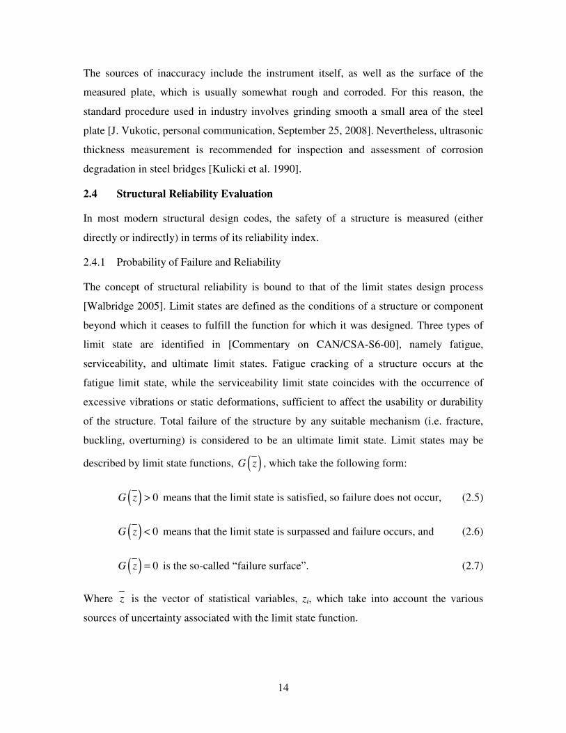
The sources of inaccuracy include the instrument itself, as well as the surface of the

measured plate, which is usually somewhat rough and corroded. For this reason, the

standard procedure used in industry involves grinding smooth a small area of the steel

plate [J. Vukotic, personal communication, September 25, 2008]. Nevertheless, ultrasonic

thickness measurement is recommended for inspection and assessment of corrosion

degradation in steel bridges [Kulicki et al. 1990].

2.4 Structural Reliability Evaluation

In most modern structural design codes, the safety of a structure is measured (either

directly or indirectly) in terms of its reliability index.

2.4.1 Probability of Failure and Reliability

The concept of structural reliability is bound to that of the limit states design process

[Walbridge 2005]. Limit states are defined as the conditions of a structure or component

beyond which it ceases to fulfill the function for which it was designed. Three types of

limit state are identified in [Commentary on CAN/CSA-S6-00], namely fatigue,

serviceability, and ultimate limit states. Fatigue cracking of a structure occurs at the

fatigue limit state, while the serviceability limit state coincides with the occurrence of

excessive vibrations or static deformations, sufficient to affect the usability or durability

of the structure. Total failure of the structure by any suitable mechanism (i.e. fracture,

buckling, overturning) is considered to be an ultimate limit state. Limit states may be

described by limit state functions, ( )G z , which take the following form:

( ) 0G z > means that the limit state is satisfied, so failure does not occur, (2.5)

( ) 0G z < means that the limit state is surpassed and failure occurs, and (2.6)

( ) 0G z = is the so-called “failure surface”. (2.7)

Where z is the vector of statistical variables, zi, which take into account the various

sources of uncertainty associated with the limit state function.

15

In [Melchers 2002] the basic reliability problem is described as having two competing

statistical variables: the resistance, R, and the applied load, S. The corresponding limit

state function and expression for the probability of failure, pf, is as follows:

( )( ) ( )0 0fp P G z P R S= < = − < (2.8)

The probability density functions (PDF) for S, R, and ( )G z are plotted in Figure 2.6. In

this figure, the bold symbols are vectors, and therefore: G(z) = ( )G z .

Figure 2.6: Probability curves [Walbridge 2005]

The pf is the area under the PDF of ( )G z for which ( ) 0G z < . If the distributions for S

and R are both normal, then the pf can be calculated as follows:

( ) ( )βσσ

µµ−Φ=

��

�

�

��

�

�

+

−−Φ=

22SR

SRfp (2.9)

where �S and �R are the means, and �S and �R are the standard deviations of the load and

resistance variables, and ()Φ is the cumulative density function for the standard normal

distribution. Often, reliability is expressed by structural engineers in terms of the

reliability index, �. As follows from Equation 2.9,

( )fp1−Φ−=β (2.10)

16

As can be seen in Figure 2.6, this index can be understood as the distance between the

mean of the ( )G z distribution and the origin, divided by the standard deviation,

( )( )G zσ . The pf for a more general case can be expressed as follows:

( )( ) ( )( ) 0

0 ...f

G z

p P G z f z dz<

= < = � � (2.11)

In other words, given a limit state function, ( )G z , containing n statistical variables, zi,

the pf is equal to the volume in n-dimensional space under the portion of the joint PDF,

( )f z , for which ( ) 0G z < . In order to solve the integral in Equation 2.11, one of two

approaches is usually applied: numerical methods such as Monte Carlo simulation (MCS)

or analytical methods such as the First Order Reliability Method (FORM) [Walbridge

2005].

2.4.2 Reliability in the Bridge Code

The safety philosophy of the [CAN/CSA S6-06] is to have a consistent level of risk to life

for each bridge element. The level of risk is equal, by definition, to the probability of

failure multiplied by the cost of failure. In [CAN/CSA S6.1-00] (see also Figure 2.7), the

cost of failure of a bridge element is related to the likelihood of the element failure

leading to loss of life. A consistent level of risk is maintained if a higher probability of

failure is accepted in the elements whose failure will not result in a loss of life, or a lower

probability of failure is accepted in the elements whose failure might result in a loss of

life. Likewise, a structural element that receives frequent inspections, shows warning

signs if approaching failure, or is capable of redistributing its load to other elements will

be less likely to cause loss of life.

17

Figure 2.7: Relationship between risk and probability of failure [CAN/CSA S6.1-00]

In the [CAN/CSA S6-06]-recommended procedure for bridge evaluation, the level of

safety is measured using the reliability index, �, which is inversely related to the notional

probability of failure. The notional probability of failure is calculated using the life safety

criterion of CSA S408-1981:

nW

AKPf = (2.12)

Where Pf is the probability of failure, A is an activity factor taking into account the risk

involved in activities associated with the structure, K is a calibration factor, W is a

warning factor, and n is an importance factor. For determining a structure’s capacity to

carry vehicle trains, two-unit vehicles, and single-unit vehicles, in normal traffic, A is 3.0,

K is 10-4, W is 1.0, and n is 10. Together, these give a Pf of 9.5 x 10-5; this is the target Pf

for a structure. Table 2.1 relates the values of the reliability index to the notional

probability of failure values, based on a probability distribution where the probability of

failure is normally distributed [CAN/CSA-S6.1-00]. Using Table 2.1 or Equation 2.10, a

probability of failure, Pf of 9.5 x 10-5 corresponds with a reliability index of 3.73.

18

Table 2.1: Notional probability of failure for various reliability indices, based on the normal

probability curve [CAN/CSA-S6.1-00]

Reliability Index, � Notional Probability of Failure, Pf

2.00 2.3 x 10-2 or 1:44

2.25 1.2 x 10-2 or 1:81

2.50 6.2 x 10-3 or 1:160

2.75 2.8 x 10-3 or 1:360

3.00 1.4 x 10-3 or 1:740

3.25 5.6 x 10-4 or 1:1800

3.50 2.3 x 10-4 or 1:4300

3.75 8.8 x 10-5 or 1:11,000

4.00 3.2 x 10-5 or 1:31,500

4.25 1.1 x 10-5 or 1:93,500

4.50 3.4 x 10-6 or 1:294,000

2.5 Structural Analysis Models of Corroding Steel Bridges

Several studies have been performed over the last two decades that examined the effects

of progressive corrosion on bridge reliability. All of the studies mentioned here focus on

the time-variant reliability of simply-supported composite I-girder bridges, but they look

at different aspects of the structures and how progressive corrosion affects their

reliability. They also consider different girder regions that can be affected by corrosion.

2.5.1 Research of J.R. Kayser

In [Kayser 1988, Kayser & Nowak 1989], the examined structures are two-lane bridges

with five I-girders, ranging from 12.2 m to 30.5 m in length. A cross section of the

examined bridge type is shown in Figure 2.8.

19

Figure 2.8: Steel I-girder bridge cross section [Kayser 1988]

The bridge has a composite section, with a 190 mm thick, 27.6 MPa concrete slab. Since

the number of girders is constant, the girder size is varied with the bridge length, from

W610x113 for the 12.2 m bridge to W920x345 for the 30.5 m bridge. The girders are

hot-rolled and composed of 250 MPa steel. Kayser apply the standard equation (see

Equation 2.3) in his corrosion penetration models. Regarding the assumed corrosion

location, for the majority of the span, general thickness loss is assumed to occur to the top

of the bottom flange and the bottom quarter of the web (Figure 2.9). However, at the

supports, the web is assumed to corrode over its entire depth.

Figure 2.9: Typical corrosion locations assumed by [Kayser 1988]

Kayser [1988] consider the effect of corrosion on the flanges and webs of the girders, but

not on the connections or secondary members such as cross-bracing. They also ignore the

problem of corrosion fatigue. The failure modes considered include shear, moment, and

bearing, since they have the greatest effect for single-span I-girders.

20

In Kayser [1988], it is found that bearing and shear usually govern at high levels of

corrosion since the resistances are dependent upon the web, which is thinner and more

sensitive to thickness loss due to corrosion. Also, elements in compression are more

sensitive since they become more susceptible to buckling.

Figure 2.10 shows the reliability predictions for a 12.2 m long bridge.

Figure 2.10: Reliability of a 12.2 m long bridge [Kayser 1988]

Figure 2.11 shows the reliability predictions for a 30.5 m long bridge.

Figure 2.11: Reliability of a 30.5 m long bridge [Kayser 1988]

As can be seen from these figures, the shorter span bridge is more susceptible to capacity

loss over time; this is a direct result of the fact that bearing stiffeners are not required for

the shorter bridge, but if the bridge is thus unfitted, it becomes susceptible to failure in

the bearing mode in a relatively short amount of time.

21

It was also found that the thickness loss exponent B is the most influential parameter in

the corrosion rate model. The variation of B had a significant effect on the reliability

fraction, �/�0, of a bridge, far more so than A, as is shown in Figure 2.12.

Figure 2.12: Sensitivity study of model parameters [Kayser & Nowak 1989]

Also presented in this figure are the effects of varying the shear distribution parameter

(SF) and the bearing plate coefficient (k). Figure 2.13 shows the reliability performance

of an 18 m long span in different corrosion environments.

Figure 2.13: 18 m long span in different environments [Kayser & Nowak 1989]

The bridge reliability is not significantly affected by the rural corrosion rate, but the

effects of the urban and marine corrosion rates are significant. Note that the reliability

analyses in this study were performed for regular carbon steel girders.

22

2.5.2 Research of A.A. Czarnecki

[Czarnecki 2006, Czarnecki & Nowak 2006] looked at bridges from 12.2 m to 42.7 m in

length, supported by four to six steel I-girders. Cross-sections are shown in Figure 2.14.

Figure 2.14: Steel I-girder bridge cross sections [Czarnecki & Nowak 2006]

Czarnecki examined bridges of the three cross sections shown for six different lengths

ranging between 12.2 m to 42.7 m. For each section type and span, he also used different

girder sizes to create structures with reliability indices under, over, and equal to the target

reliability index (�T).

Regarding the corrosion penetration rate equation, in [Czarnecki & Nowak 2006] the

modelling is done assuming painted carbon steel, and so the corrosion penetration line is

essentially divided into concave and convex parts to take into account, first, the

degradation of the coating, and after this, the progression of corrosion penetration. This is

shown in Figure 2.15.

23

Figure 2.15: Corrosion rates for research of [Czarnecki & Nowak 2006]

The corrosion penetration curves in Figure 2.15 were selected based on both field

observations and the data in [Albrecht & Naeemi 1984]. The high corrosion rate

represents an industrial or marine environment or one where de-icing salts are used, while

the low corrosion rate is for dry areas with little chemical contamination.

Regarding the locations on the bridge subject to corrosion, Czarnecki thought the

approach used in [Kayser 1988, Kayser & Nowak 1989] was too refined; basically, there

are too many variables that determine corrosion spread and penetration, and so the

prediction is not realistic, he argues. Preferring a more general approach, [Czarnecki

2006] supposes surface loss due to corrosion over the entire web and top of the bottom

flange for the whole bridge span, as shown in Figure 2.16.

Figure 2.16: Corrosion location [Czarnecki 2006]

24

Czarnecki’s work examined the effects of corrosion on the reliability of the system as a

whole rather than any part of it. Depending on the configuration of the structure,

considering system behaviour can result in a more reliable structure due to the fact that

when a member is stressed beyond its capacity it is not removed from the structure;

rather, the excess loads are distributed elsewhere. The type of computation required for

this analysis is considerably complex; in this case, bridge models were built using a

dedicated structural engineering program. A nonlinear model was applied to account for

stress and load redistribution that occurs when a member progresses from the state of

local yielding to ultimate, and from there to where the bridge fails.

Three limit states were checked: member failure, total bridge collapse, and a

serviceability limit state (i.e. excessive deflection equal to 0.0075 of the span length).

Analyses were performed for ultimate limit states (moment and shear) and serviceability

(deflection), and structural performance was measured in terms of the reliability index.

It was found that reliability models provide a real benefit by facilitating estimations of the

time-dependent bridge deterioration. While the low corrosion rate had a negligible effect

on the bridge performance, a high corrosion rate significantly reduced the bridge capacity

over time. It was further found that bridge reliability decreases much more rapidly for

shorter spans compared to longer ones. Figure 2.17, Figure 2.18, and Figure 2.19 show

the decreasing system reliability of bridges as their spans become shorter.

Figure 2.17: System reliability for long span bridge [Czarnecki & Nowak 2006]

25

Figure 2.18: System reliability for medium span bridge [Czarnecki & Nowak 2006]

Figure 2.19: System reliability for short span bridge [Czarnecki & Nowak 2006]

A sensitivity analysis was also performed by Czarnecki, which showed that the statistical

parameters related to the structural steel had a more noticeable effect on the structural

behaviour than those parameters related to the concrete slab.

2.5.3 Research of M.S Cheung and W.C. Li

Cheung and Li [2001] looked at bridges of varying lengths with five rolled steel or built-

up I-girders. Figure 2.20 below shows the arrangement of the girders and concrete slab.

26

Figure 2.20: Structural arrangement [Cheung & Li 2001]

The same corrosion model (i.e. corrosion rate and location) as the one used by Kayser

was applied here. The finite strip method was used in [Cheung & Li 2001] to determine

the effect of corrosion on the serviceability of the structure, i.e. based on its deflection.

The finite strip method uses beam eigenfunctions to express the longitudinal variation of

displacements. This method requires the creation of a finite element model of the bridge

cross-section in order to develop a stiffness matrix for the section as a whole. Figure 2.21

shows a typical finite strip model of the bridge section. As an analysis method, the finite

strip method is more universal and more accurate than beam theory, and requires much

fewer calculations than a full finite element model.

Figure 2.21: Finite strip model [Cheung & Li 2001]

In [Cheung & Li 2001], the A and B corrosion parameters, the thickness of the slab, and

the moduli of elasticity of steel and concrete were varied in order to determine their effect

on the time-dependent bridge reliability. Based on this work, it was found that, even if the

nominal corrosion rate was low, corrosion still had a profound effect on the bridge

serviceability, due to the fact that some corrosion rates had a large variance, so it was still

possible to have high rates of corrosion penetration on occasion.

27

2.5.4 Research of P. Laumet

Laumet [2006] focussed on the deflection limit state of composite girder bridges. As with

the above studies, the structures were single-span, I-girder bridges. Bridges with span

lengths between 15.3 and 39.7 m, and girder spacing between 1.83 and 3.66 m, were

considered. His models take into account nonlinear behaviour of the structural materials,

i.e., the creep and shrinkage of the concrete slab and plastification of the steel girders. In

[Laumet 2006] the logarithmic power model (see Equation 2.3) is used to predict the

corrosion penetration. Only general corrosion is considered.

It is found that corrosion has a significant effect on the reliability of the bridge.

Interestingly, it is also suggested that the deflection limit state should not be considered

as a reliability limit state; on the other hand, steel yield is a valid reliability limit state,

according to this reference. The reason for this is that the deflection limit state (L/800 is

used here) does not correspond to any actual structural state, and since the bridge will

frequently experience traffic loads that are larger than those predicted by the design

codes, the structure’s reliability index will show negative values.

2.5.5 Research of C.H. Park

The purpose of the research done by Park [1999] was to determine the effects of time

dependent loads and corrosion on bridge reliability. The structures examined in this

reference were composite I-girder bridges, between 10 and 30 m long, 12 m wide, and

supported by a varying number of girders. The bridge structures were also examined as

systems to determine their safety reserves as such. The model used in [Park 1999] is

shown in Figure 2.22.

Figure 2.22: Corrosion locations [Park 1999]

28

As a preliminary part of his research, Park varied the ��L value (shown in Figure 2.22)

between 1.0 and 3.0 m, and found that doing so did not affect the reliability of his bridge

model. The same corrosion model is used here as in [Czarnecki & Nowak 2006] (see

Figure 2.15). Failure due to shear was found to be a more immediate threat to the

structure than that due to moment. In fact, for short-span bridges, shear buckling is the

governing failure mode at the maximum lifetime of the bridge. Sections with thinner

webs are obviously more susceptible to web failure, and so it is recommended that web

stiffeners be used. Importantly, it was found that the reliability of the bridge as a system

was significantly higher than that of the individual components.

2.5.6 Other Research

Included in this section are structural reliability studies that either did not consider the

effects of corrosion or did not examine the bridge structure as a whole.

Research of Sarveswaran et al.

Sarveswaran et al. [1998] also looked at the effect of corrosion penetration on component

reliability: rather than considering composite I-girder structures, the research examined

steel members alone. However, interval probability theory was used to determine the

system reliability. In [Sarveswaran et al. 1998] only structures with known amounts of

section loss due to corrosion are considered, due to the difficulty and uncertainty of

predicting future corrosion penetration. For the general model, section loss occurs to the

entire steel section, but at an advanced rate for the bottom ¼ of the web and the flange.

Corrosion was also expected to attack both the top and bottom surfaces of the flanges. A

diagram of the resulting beam section is shown in Figure 2.23.

29

Figure 2.23: Beam section [Sarveswaran et al. 1998]

The findings of [Sarveswaran et al. 1998] are that the most critical failure mode affecting

the beam is lateral-torsional buckling, due in part to beam coping. This is followed by

shear, since the loss of material affects the bottom quarter of the web most directly, and

then by moment, since section loss to the compression flange is less significant.

Research of Eamon and Nowak

Eamon and Nowak [2004] attempted to evaluate the effect of secondary elements, such as

sidewalks and barriers, on the system reliability of girder bridges, assuming these

elements participate in resisting live loads due to truck traffic, but also contribute to the

dead load on the span. The effect of corrosion penetration over time was not considered.

The study considered two-lane structures with varying numbers of I-girders and varying

in length from 10 to 50 m. The results of [Eamon & Nowak 2004] show that the

secondary elements did affect the reliability of the bridge structural systems. The effects

varied with bridge span and girder spacing. Short-span structures showed the largest

increases in reliability index, due to the additional capacity provided by the edge-

stiffening elements. Figure 2.24 shows the effect of span length on reliability.

30

Figure 2.24: Reliability data for varying spans with 2 m girder spacing [Eamon & Nowak 2004]

Girder spacing was also found to influence reliability, but to a lesser degree. Since the

number of girders affects system redundancy, structures with more, or more closely-

spaced, girders had the highest reliability indices. Figure 2.25 shows these results.

Figure 2.25: Reliability data for 50 m span [Eamon & Nowak 2004]

2.6 Summary

2.6.1 Corrosion of Weathering Steel

As mentioned earlier, there are some differing views on the exact nature and mechanism

of corrosion penetration in weathering steel. Nevertheless, there is a consensus that its

alloy content enables weathering steel to form a dense, uniform layer, which protects it

from ingress of air, moisture, and pollutants that cause corrosion and lead to section loss.

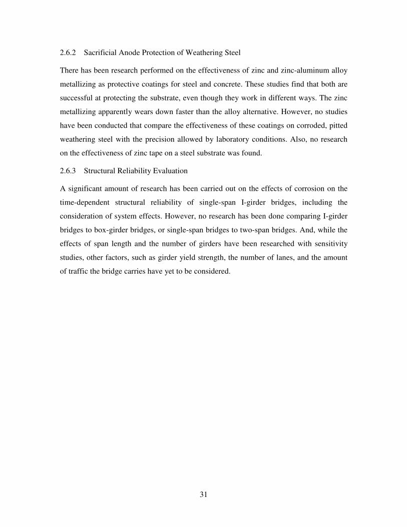
31

2.6.2 Sacrificial Anode Protection of Weathering Steel

There has been research performed on the effectiveness of zinc and zinc-aluminum alloy

metallizing as protective coatings for steel and concrete. These studies find that both are

successful at protecting the substrate, even though they work in different ways. The zinc

metallizing apparently wears down faster than the alloy alternative. However, no studies

have been conducted that compare the effectiveness of these coatings on corroded, pitted

weathering steel with the precision allowed by laboratory conditions. Also, no research

on the effectiveness of zinc tape on a steel substrate was found.

2.6.3 Structural Reliability Evaluation

A significant amount of research has been carried out on the effects of corrosion on the

time-dependent structural reliability of single-span I-girder bridges, including the

consideration of system effects. However, no research has been done comparing I-girder

bridges to box-girder bridges, or single-span bridges to two-span bridges. And, while the

effects of span length and the number of girders have been researched with sensitivity

studies, other factors, such as girder yield strength, the number of lanes, and the amount

of traffic the bridge carries have yet to be considered.

32

CHAPTER 3: TESTS AND PROCEDURES

This chapter describes the laboratory tests conducted to assess and evaluate the accuracy

of UTG measurements of corroded bridge plates and the benefit of metallizing and zinc

tape as a means of reducing the rate of corrosion.

3.1 Ultrasonic Thickness Measurements

3.1.1 Background

Ultrasonic thickness (UT) measurement is the most common method of measuring the

thickness of steel plate on a structure. The technique is as follows: a transducer is put in

contact with the surface of the material being measured. The quality of the contact can be

increased by the use of a couplant, usually a gel. The transducer emits ultrasonic waves

that pass from a transmitter (T) through the material and reflect off the opposite wall and

back to a receiver (R), providing there are no discontinuities or cracks that might first

intercept the waves [Antaki 2005]. Figure 3.1 shows a diagram of this.

Figure 3.1: Explanation of ultrasonic thickness measurement

The main advantage of this system (versus the use of callipers, for example) is that it

needs access to only one side of the plate being measured. However, there is significant

uncertainty about what is actually being measured when the probe is placed on a heavily

pitted surface or if there is a corrosion layer between the probe and the steel.

The goal of the research into ultrasonic thickness measurements performed for the current

study was to determine the effectiveness and accuracy of UTGs when being applied to

corroded steel plate. The effect of corrosion products (on either side of the plate) on the

thickness measurement was studied, specifically whether the corrosion product was

included in the thickness measurement of the steel. Also, the effect of pitting on the

measurements was examined. As shown in Figure 3.2, it was necessary to design a test to

33

examine the effect of pitting, not only on the face being measured (thereby denying the

UTG a smooth working surface), but also on the opposite face, in order to determine

whether the distance to the pit or to the opposite face is what is being measured.

Likewise, clear information could not be found in the existing literature on the effect of

corrosion product (rust) on the reported thickness measurement.

���������

�����

��������

����� �

�������

���

����

����

��������

��� �������

����������

�����

Figure 3.2: Explanation of uncertainty in ultrasonic thickness measurement.

3.1.2 Equipment

The Nova Eclipse TG110DL was the UTG used for this study; Figure 3.4 is a photograph

of this instrument. The TG110DL has a built-in microprocessor for calculating the

thickness of the material and a liquid crystal display for the visual interface. It is a

handheld unit with the transmitter and receiver contained together in the probe that is

applied to the material being tested (Figure 3.3).

Figure 3.3: UTG probe head

34

Figure 3.4: UTG and couplant

A variety of probes are available for use with this gauge, but for this project the Standard

Probe (TG506) was the only one used. The gauge functions by sending a short ultrasonic

pulse into the material and measuring the amount of time it takes for the signal to return

after echoing off the back surface of the material. In calculating the material thickness,

the gauge takes into account the characteristic ultrasonic velocity of the material. The

gauge user’s manual recommends a longitudinal ultrasonic velocity of 5.9 mm/�s for

mild steel, and this is the value that is used for all measurements. The UTG results

compared well with those provided by digital callipers and the Coordinate Measuring

Machine described below. The couplant used was Sonotech Ultragel II, an ultrasonic

couplant with a temperature range of -20° to 150° C.

A Mitutoyo BHN305 Coordinate Measuring Machine (CMM) was used to obtain

measurements of the plate thickness with which the ultrasonic thickness measurements

could be compared. The CMM (Figure 3.5) is a computer controlled measurement device

used to measure the dimensions of three dimensional objects.

35

Figure 3.5: Coordinate Measuring Machine

It uses a needle-like probe to mechanically determine the x-, y- and z-coordinates of a

point on the surface of the specimen. The probe can be manipulated directly by the user,

or it can be directed to measure the object at a series of set locations or in a preset grid. It

is programmable, so the user can enter a grid and let it run automatically.

The CMM does point measurements only, and not a continuous scan along a line. It is

calibrated by measuring specimens of known dimensions. The surface profile

measurements obtained with the CMM can be directly translated into thickness

measurements if one side of the specimen is polished flat.

By comparing the UTG measurements with the physical measurements made using the

CMM, it is possible to determine the level of accuracy provided by the UTG and, in

particular, to determine the effects of pitting and corrosion product (on the front or back

surfaces of the plate) on the measurements recorded by the UTG probe.

36

3.1.3 Tests

Machined Groove Thickness Measurement Test

Prior to measuring the thicknesses of corroded plate specimens, it was decided to test the

ultrasonic gauge on a machined groove of known geometry. The steel used in this test

was the taken from the “new weathering steel” sample provided by Algoma, as discussed

in Section 3.3, with the corrosion product removed and all of the surfaces of the specimen

machined smooth. For this test, the weathering steel specimen was first machined to a

constant thickness. A groove (depth = 1.854 mm, radius = 3.175 mm) was then cut across

the specimen to simulate a deep pit in the steel (Figure 3.6).

Figure 3.6: Steel specimen with groove

The specimen was then mounted onto an electronic height gauge that permitted vertical

translation while measuring the change in vertical position to the hundredth of a

millimetre. The UTG probe head was mounted on a three-prong swivel clamp and a

magnetic clamp stand, allowing the sensor to be in contact with the specimen at all times.

The full test setup can be seen in Figure 3.7.

37

Figure 3.7: Machined groove thickness measurement test setup

To record the data, an arbitrary initial point above the groove was chosen and the

thickness was recorded. The specimen was then moved across the UTG probe head and

the position and the thickness value recorded at each location. This process was repeated

until a complete line including the machined groove was measured. This test was run

with the UTG probe head mounted in two orientations, termed “parallel” and

“perpendicular” (see Figure 3.8). The results of this test are presented in Chapter 4.

Figure 3.8: Parallel (left) and perpendicular (right) orientations of probe head

Specimen

UTG probe

Height gauge

Swivel clamp

UTG

38

For this test, a circular irregularity was measured because it approximates the expected

shape of a corrosion pit; however, for the purposes of the structural research, the shape of

the pit is not as important as its depth.

Corroded Specimen Thickness Measurement Tests

The objective of the next series of tests was to determine the accuracy and limitations of

the UTG when used to measure heavily corroded piece of weathering steel, specifically in

view of the concerns discussed in Section 3.2.1.

For these tests, two types of specimens were considered, those with heavy corrosion and

those with light corrosion. Figure 3.9 and Figure 3.10 are photos of typical specimens.

Note that the heavily corroded specimens were “old steel” coupons cut from a larger

sample taken from the Big Otter Creek Bridge; the lightly corroded specimens were “new

steel” coupons cut from a sample provided by Algoma. The specimens were machined to

a length of 90 mm and a width of 45 mm. The top, more heavily corroded, surface was

initially left untouched, while the bottom surface was milled smooth.

Figure 3.9: “Old steel” specimen with heavy corrosion (old steel)

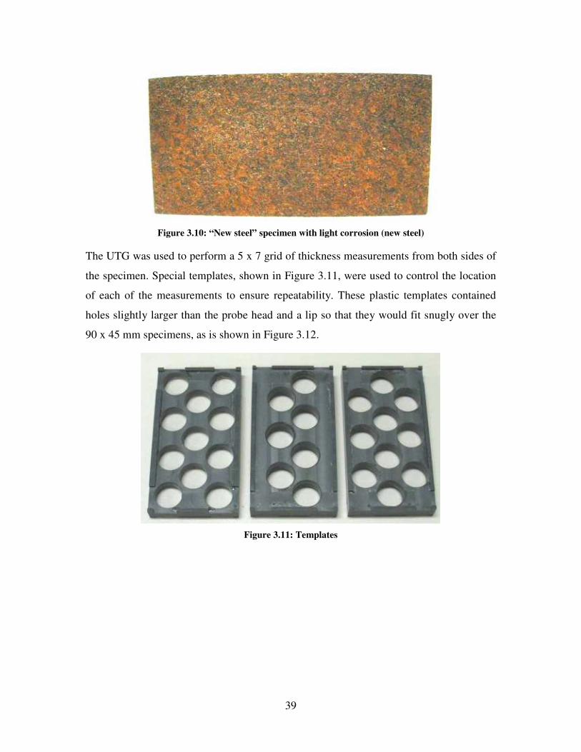
39

Figure 3.10: “New steel” specimen with light corrosion (new steel)

The UTG was used to perform a 5 x 7 grid of thickness measurements from both sides of

the specimen. Special templates, shown in Figure 3.11, were used to control the location

of each of the measurements to ensure repeatability. These plastic templates contained

holes slightly larger than the probe head and a lip so that they would fit snugly over the

90 x 45 mm specimens, as is shown in Figure 3.12.

Figure 3.11: Templates

40

Figure 3.12: UT measurements with templates

Once the UT measurements were complete, the CMM was used to collect a 5 x 7 grid of

thickness measurements at the center of each UTG measurement point. After these

measurements were taken, the corrosion product was removed from each specimen by

“pickling” as per [ASTM G1-03]. The clean specimens (Figure 3.13 and Figure 3.14)

were examined under a microscope to ensure that the corrosion product was fully

removed. Once cleaned, the UTG and CMM measurements were repeated.

Figure 3.13: Pickled specimen with heavy corrosion (old steel)

41

Figure 3.14: Pickled specimen with light corrosion (new steel)

In addition, the CMM was used to collect a data set in a 13 x 13 grid with a spacing of

1.5 mm between each measurement; the centre of this grid was located at the centre of

the specimen. The results of this series of tests are also summarized in Chapter 4.

3.2 Corrosion Testing

3.2.1 Background

The objective of the corrosion testing performed for the current study was to examine the

corrosion resistance of three different coating products. The test program was also

designed to examine the effect of varying the level of sandblasting, the steel type, and the

degree of corrosion damage to the surface prior to the coating.

3.2.2 Test Program

The test matrix for the corrosion testing is shown in Table 3.1. Five specimens of each

type were used to ensure statistical viability.

42

Table 3.1: Corrosion test matrix

Group Material Corrosion Treatment Coating Count

1 Old steel Heavy Full sandblast None 5

2 New steel Light Full sandblast None 5

3 New steel Light Full sandblast Aluminum alloy metallizing 5

4 Old steel Heavy Full sandblast Zinc metallizing 5

5 New steel Light Full sandblast Zinc metallizing 5

6 Old steel Heavy Half sandblast Zinc metallizing 5

7 New steel Light Half sandblast Zinc metallizing 5

8 Old steel Heavy Full sandblast Zinc tape 5

9 New steel Light Full sandblast Zinc tape 5

10 Old steel Heavy Half sandblast Zinc tape 5

11 New steel Light Half sandblast Zinc tape 5

The test regimen chosen for the corrosion test was [SAE J2334]. This test regimen was

originally designed for testing the corrosion resistance of automobile parts; however, it

was used in the current study because of its known ability to induce significant corrosion

thickness loss over a relatively short test duration, and due to the smaller area of steel

required for the specimens. According to this regimen, this test follows a 24-hour cycle,

as shown in Figure 3.15.

43

Figure 3.15: Test cycle [SAE J2334]

The composition of the [SAE J2334] immersion solution is as follows:

• 0.5 wt% NaCl

• 0.1 wt% CaCl2

• 0.075 wt% NaHCO3

Each of these constituents was obtained in solid (powder) form and dissolved in the

distilled water that comprised the remainder of the solution.

Conductivity and pH were tested on a weekly basis to ensure the quality of the solution.

An Orion Model 710A pH/ISE meter was used to test the pH of the solution; a Hach

conductivity/TDS meter was used to monitor its conductivity.

3.2.3 Test Equipment

The test regimen was imposed by placing the specimens in an Ascott Cyclic Corrosion

Test Chamber (model CC450). The system, which has a 450 L capacity, has two

components: a corrosion chamber and a solution reservoir (Figure 3.16 and Figure 3.17).

Humid cycle 50 �C & 100% RH

6 hours

Immersion cycle Ambient temp and RH

15 minutes

Dry cycle 60 �C & 50% RH

17 hours & 45 minutes

44

Figure 3.16: Corrosion chamber

Figure 3.17: Solution reservoir

The Ascott system is programmable through a touch screen, and automatically adjusts the

temperature, humidity, and immersion of the specimens. Its capacity for automatic

operation means that it could operate continuously.

Test racks for the specimens were cut from black ABS plastic tubing. Figure 3.18 shows

a diagram of the test rack (dimensions are in mm). The specimens were placed in a

random order on the racks inside the corrosion tester. Once per week they were removed

to be weighed and photographed (this was reduced to once per two weeks at the 120-

cycle mark); they were then returned to the machine in a different order to ensure that

their location inside the tester would not be a factor in their corrosion rate.

45

Figure 3.18: Test rack diagram

3.2.4 Specimens

Steel for the corrosion specimens came from two sources. The “old steel”, provided by

the MTO, came from a splice plate from the Big Otter Creek Bridge on King’s Highway

No. 3 near Tillsonburg, Ontario. Figure 3.19 shows a photo of the old steel in its “as

received” state.

Figure 3.19: Old steel sample provided by MTO

The bridge drawings specify CSA G40.11 Grade 50A (yield strength, Fy = 345 MPa)

atmospheric corrosion resisting steel. Inspections indicated this I-girder bridge, which is

near Tillsonburg, Ontario, was experiencing very high corrosion rates and, as part of the

repair procedure, some of the splice plates, as well as parts of the I-girder, were removed

and replaced. This steel was observed to be heavily pitted and had lost some of its

section. The section loss could be deduced because the steel under the bolt holes was not

corroded, and the steel around them was much less thick. Figure 3.20 shows a photo of

the profile of a pickled specimen cut from the old steel splice plate.

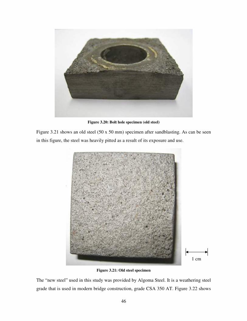
46

Figure 3.20: Bolt hole specimen (old steel)

Figure 3.21 shows an old steel (50 x 50 mm) specimen after sandblasting. As can be seen

in this figure, the steel was heavily pitted as a result of its exposure and use.

Figure 3.21: Old steel specimen

The “new steel” used in this study was provided by Algoma Steel. It is a weathering steel

grade that is used in modern bridge construction, grade CSA 350 AT. Figure 3.22 shows

1 cm

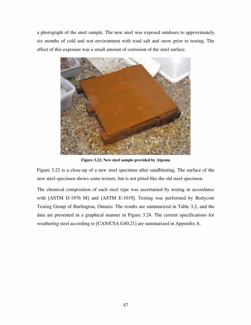
47

a photograph of the steel sample. The new steel was exposed outdoors to approximately

six months of cold and wet environment with road salt and snow prior to testing. The

effect of this exposure was a small amount of corrosion of the steel surface.

Figure 3.22: New steel sample provided by Algoma

Figure 3.23 is a close-up of a new steel specimen after sandblasting. The surface of the

new steel specimen shows some texture, but is not pitted like the old steel specimen.

The chemical composition of each steel type was ascertained by testing in accordance

with [ASTM D-1976 M] and [ASTM E-1019]. Testing was performed by Bodycote

Testing Group of Burlington, Ontario. The results are summarized in Table 3.2, and the

data are presented in a graphical manner in Figure 3.24. The current specifications for

weathering steel according to [CAN/CSA G40.21] are summarized in Appendix A.

48

Figure 3.23: New steel specimen

Figure 3.24: Percent composition of alloying elements

1 cm

49

Table 3.2: Steel compositions, wt%

Element Old Steel, % New Steel, %

Al 0.05 0.03

C 0.15 0.06

Ca < 0.005 < 0.005

Cr 0.31 0.49

Cu 0.30 0.24

Mn 0.87 1.16

Mo 0.02 0.01

Nb < 0.005 < 0.005

Ni 0.32 0.29

P 0.005 0.011

S 0.024 0.006

Si 0.15 0.40

V 0.012 0.053

The old and new steels have a chemical composition that would qualify them as 350A or

350 AT steels (see Appendix A, Table A.1). The new steel contains significantly larger

amounts of chromium, manganese, silicon and vanadium, but smaller amounts of carbon,

aluminum, copper, and sulphur. The effects of these alloying elements are summarized as

follows [Kulak & Grondin 2006, Albrecht & Naeemi 1984]: carbon increases the steel’s

strength and hardness, but tends to decrease its ductility and toughness. Manganese

increases strength and hardness in a similar manner, except that it also increases the

toughness. Chromium, copper, nickel, and silicon all serve to increase the corrosion

resistance of the steel; manganese likewise has a beneficial effect on the corrosion

resistance. Silicon and aluminum may also be present as deoxidizers, while vanadium is

an effective precipitation strengthener. Phosphorus and sulphur are considered to be

impurities and should be minimized if possible.

50

3.2.5 Pre-treatment

The old and new steel specimens were pretreated by sandblasting performed by a

licensed contractor: Reitzel Brothers Sandblasting of Ontario. Thirty-five of the 55 total

samples were sandblasted to a level compliant with [SSPC-SP 5/NACE No. 1]. The

remainder of the samples were sandblasted to approximately half this level. The intent of

this was to simulate an improperly sandblasted piece of steel in order to test the effect of

sandblasting on coating effectiveness. In addition, it was thought that, if both specimen

types performed equally well, then perhaps a lower cleaning criterion could be permitted,

thereby reducing the preparation cost for the coating procedure.

3.2.6 Coatings/Treatment

As indicated in Table 3.1, three different coating products were applied to the weathering

steel specimens. Each of these products operates as a sacrificial anode. All of the tape and

metallizing products and procedures used for the current study were supplied and applied

by Vector Corrosion Technologies.

Galvanic (Zinc) Tape

The tape product tested was Galvanode® ZincTape, and is comprised of three layers: the

first (outer) layer is a topcoat of PVC, followed by a layer of high purity zinc (min.

99.99% zinc). The third is a layer of electro-conductive, pressure sensitive adhesive (the

electrical conductivity is required to produce an electrical contact between the surface of

the steel and the zinc tape). The adhesive is advertised to be capable of resisting a

continuous temperature of 120°C, so there was no reason to expect a thermal breakdown

of the adhesive to have an effect on the tape’s performance.

The application of the tape is a straightforward process. Care has to be taken to prepare

the surface correctly, either by scrubbing with a steel brush or sandblasting. Thin strips of

tape have to be applied at the edges of the steel first, before the wider strips of tape can be

used to cover up large, flat spaces between the edge strips.

Metallizing

Two metallizing products were examined in this study: zinc and aluminum alloy (see

Table 3.1). The zinc metallizing product, like the zinc tape, is composed of high purity

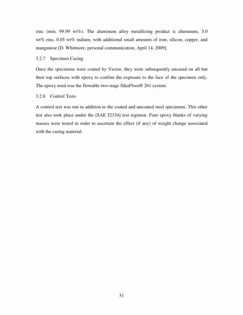
51

zinc (min. 99.99 wt%). The aluminum alloy metallizing product is aluminum, 5.0

wt% zinc, 0.05 wt% indium, with additional small amounts of iron, silicon, copper, and

manganese [D. Whitmore, personal communication, April 14, 2009].

3.2.7 Specimen Casing

Once the specimens were coated by Vector, they were subsequently encased on all but

their top surfaces with epoxy to confine the exposure to the face of the specimen only.

The epoxy used was the flowable two-stage SikaFloor® 261 system.

3.2.8 Control Tests

A control test was run in addition to the coated and uncoated steel specimens. This other

test also took place under the [SAE J2334] test regimen. Four epoxy blanks of varying

masses were tested in order to ascertain the effect (if any) of weight change associated

with the casing material.

52

CHAPTER 4: TEST RESULTS AND INTERPRETATION

In this chapter the results of the tests made with the ultrasonic thickness gauge (UTG) are

presented and analysed. Also presented are the results of the corrosion test which was

performed with uncoated, metallized, and taped steel specimens.

4.1 Ultrasonic Thickness Measurement Tests

4.1.1 Machined Groove Test

In the machined groove test, the UTG was tested on a steel specimen with a machined

semicircular groove. The test was run with the probe head in two different orientations,

with the transmitter and receiver aligned parallel and perpendicular with respect to the

gauge travel direction (see Figure 3.8).

Results

Figure 4.1 shows the thickness measurements made by the UTG with the probe in the

parallel and perpendicular orientations, in comparison with the physically measured

dimensions of the groove.

Figure 4.1: Machined groove test results compared with theoretical groove data.

The curve representing the physical measurements is based on thickness measurements of

the specimen, measurements of width and depth of the groove, and an assumed circular

cross section of the groove (the groove was drilled, so this assumption is expected to be

realistic). The maximum depth and width measurements are presented in Table 4.1.

53

Table 4.1: Groove test measurements.

Measurement device Depth (mm) Top width (mm)

Physical 1.85 5.61

Parallel 1.85 8.22

Perpendicular 1.87 13.70

The UTG accurately measures the depth of the groove, regardless of the orientation of the

probe; however, the measured width of the groove varies substantially and is not

accurate.

Interpretation

The UTG works by transmitting and receiving ultrasonic pulses (see Section 3.2.1).

These pulses, in the form of waves, return to the probe after reflecting from a

discontinuity in the transmitting medium. They return at different intervals, depending on

the distance travelled (assuming the transmitting medium is continuous); the UTG

displays the calculated thickness based on the first wave to return. Once the distance to

the edge of the groove is shorter than the distance to the opposite side of the specimen,

this is the distance that is reported as the specimen thickness. Based on this assumption, a

theoretical probe reading can be calculated for a given probe position. However, only

surfaces perpendicular to the direction of the wave are able to reflect it back to the UTG

receiver. Figure 4.2 shows the direct (A) and angular (B) paths.

Figure 4.2: Ultrasonic wave paths

The shortest distance between the UTG and the opposing surface is the one used for the

shortest distance assumption. Two lines based on the calculated or theoretical probe

reading, based on the shortest distance assumption, are presented in Figure 4.2.

54

The theoretical UT values that were calculated were based on this “shortest distance”

assumption. As can be seen from Figure 4.1, there is a noticeable similarity between the

measurement made with the probe head in the perpendicular orientation and the

theoretically shortest distance. The difference between the parallel and perpendicular

orientation output is probably due to the fact that the instrument cannot register a weak

return signal in the parallel orientation. Other factors that may have had an influence on

both the parallel and perpendicular data are (1) the distance between the transducer and

receiver and (2) the shape of the ultrasonic beam produced by the transducer, which, due

to the shape of the transducer, is probably somewhat irregular.

Based on this study, it can be concluded that, the UTG output is reliable if it is being used

to measure the thickness of a metal plate that is subject to general corrosion; however, the

UTG is not well-suited for locating and measuring individual pits.

4.1.2 General Corrosion Measurement Test

In the general corrosion measurement test, the UTG was tested on steel specimens with

varying degrees of corrosion. The specimens were first measured with the corrosion

product present, and then again with the corrosion product removed by pickling. Each

specimen was measured at 35 locations, and measurements were made three times to

confirm their accuracy.

Old Steel Results

For the old steel, it proved impossible to measure the thickness from the corroded face of

the specimen due to the heavy pitting; a relatively smooth surface is required for the UTG

to take a reading. Thus, UTG readings were taken only from the back of the specimen

only, which had been milled flat. CMM measurements were taken on the corroded face,

which only measures the surface profile. However, if the side of the specimen sitting on

the CMM table is perfectly flat, then the profile measurements can be equated to

measurements of thickness. A summary of the statistical data for each of the readings is

provided in Table 4.2.

55

Table 4.2: Old steel specimen thickness measurement data

Condition Tool Value Spec. 3 (mm) Spec. 4 (mm) Spec. 5 (mm)

As received UTG Average

Std. dev.

14.12

0.22

14.21

0.11

14.35

0.18

Pickled UTG Average

Std. dev.

14.10

0.22

14.26

0.11

14.38

0.18

As received CMM Average

Std. dev.

14.33

0.26

14.54

0.29

14.73

0.31

Pickled CMM Average

Std. dev.

14.14

0.22

14.34

0.20

14.45

0.23

Figure 4.3 is a histogram showing the statistical distributions of the readings made with

the UTG, taken before the corrosion product had been removed by pickling.

Figure 4.3: Histogram of as received old steel specimen thicknesses, by UTG

There is some variation in the data, which is probably due to the fact that the different

specimens had experienced varying degrees of corrosion. Figure 4.4 is a histogram of the

data collected with the UTG applied to the same three specimens after pickling.

56

Figure 4.4: Histogram of pickled old steel specimen thicknesses, by UTG

Once again, there is a significant amount of variability between the individual specimens,

but there is also a clear similarity between Figure 4.3 and Figure 4.4. The CMM was used

to measure the same old steel specimens before and after pickling. Figure 4.5 shows a

histogram of the plate thicknesses measured with the CMM from the corroded face of the

old steel specimen before pickling. The data in Figure 4.5 collected with the CMM are

more scattered than the UTG data.

Figure 4.5: Histogram of as received old steel specimen thicknesses, by CMM

Figure 4.6 is a histogram of the data collected with the CMM from the corroded face of

the old steel specimen after pickling.

57

Figure 4.6: Histogram of pickled old steel specimen thicknesses, by CMM

Old Steel Data Interpretation

Table 4.3 contains the results of the average thickness before pickling (tas received) minus

the average thickness after pickling (tpickled), as measured with the UTG and CMM.

Table 4.3: Comparison of old steel specimen thickness measurements

�t Spec. 3 (mm) Spec. 4 (mm) Spec. 5 (mm)

tas received, UTG – tpickled, UTG, mm 0.01 -0.05 -0.01

tas received, CMM – tpickled, CMM, mm 0.19 0.20 0.28

The CMM found 0.2 to 0.3 mm of corrosion product on the face of the corroded steel

specimens on average. With the UTG, however, thickness measurements made from the

uncorroded face before and after pickling are precise to within 0.02 mm on average,

which is an acceptable error for this application. From this, it can be concluded that the

UTG does not include the corrosion product in its measurements.

New Steel Results

The new steel, lightly corroded specimens were also measured with the UTG and CMM,

both before and after pickling; however, in this case, the UTG probe was applied to the

corroded face of the steel. Due to the relatively small amount of rust present, the UTG

58

was still able to measure the specimen thickness from the corroded side. A summary of

the measurement data for the new steel specimens is available in Table 4.4.

Table 4.4: New steel specimen thickness measurement data

Condition Tool Value Specimen 3 Specimen 4 Specimen 5

As received UTG Average

Std. dev.

15.47

0.02

15.55

0.05

15.51

0.05

Pickled UTG Average

Std. dev.

15.35

0.02

15.29

0.02

15.28

0.03

As received CMM Average

Std. dev.

15.30

0.03

15.29

0.03

15.26

0.04

Pickled CMM Average

Std. dev.

15.24

0.02

15.22

0.02

15.21

0.03

Figure 4.7 is a histogram of the data collected with the UTG on the three new steel

specimens prior to pickling. The data in Figure 4.7 are quite closely grouped.

Figure 4.7: Histogram of as received new steel thicknesses, by UTG

Figure 4.8 is a histogram of the data collected with the UTG on the new steel specimens

after they have been pickled.

59

Figure 4.8: Histogram of pickled new steel thicknesses, by UTG

Once again, it is a tight group of data; however, the data are now significantly lower than

what was collected with the rust still attached to the specimens. Figure 4.9 is a histogram

of the data collected by CMM on the new steel specimen with the corrosion product still

attached.

Figure 4.9: Histogram of as received new steel thicknesses, by CMM

Once again the data are quite tightly grouped, and the values are generally lower than

those presented in Figure 4.7. Figure 4.10 is a histogram of the data collected with the

CMM on the pickled new steel specimens.

60

Figure 4.10: Histogram of pickled new steel thicknesses, by CMM

Again the data are quite tightly grouped, and in the lower range of values for these

specimens. Comparing Figures 4.9 and 4.10, it can be seen that the average thickness,

measured by the CMM, is slightly lower after the specimens are pickled.

New Steel Data Interpretation

Table 4.5 contains the average thickness before pickling minus the average thickness

after pickling, as measured with the UTG and CMM, for specimens 3, 4, and 5. Note that

in this case, all of the measurements have been made from the corroded side.

Table 4.5: Comparison of new steel specimen thickness measurements

�t Spec. 3 (mm) Spec. 4 (mm) Spec. 5 (mm)

Tas received, UTG – tpickled, UTG, mm 0.13 0.26 0.23

Tas received, CMM – tpickled, CMM, mm 0.06 0.07 0.05

It would appear from the data in Table 4.5 that the UTG overestimates the thickness of

the steel by as much as 0.2 mm, approximately four times the thickness of the corrosion

layer. This inaccuracy is caused by the rust coating on the specimen, through which the

ultrasonic waves must pass twice in order for the plate to be measured. The rust layer is

thin enough that the UTG still registers the returning energy, but is significantly less

dense than the steel and, therefore, transmits the energy at a slower rate. Table 4.6 shows

61

the differences between the measurements made with the UTG and CMM on the pickled

old steel and new steel specimens.

Table 4.6: Comparison of measurements taken with UTG and CMM on pickled specimens

tpickled, UTG – tpickled, CMM, mm Specimen 3 Specimen 4 Specimen 5

Old steel -0.04 -0.08 -0.08

New steel 0.11 0.07 0.07

In the measurements made on the old steel specimen, the UTG returned data that are on

average 0.07 mm smaller than the CMM. However, in measurements made on the new

steel specimen, the UTG data are on average 0.08 mm larger than the CMM data. There

are two possible sources of error, which are given below.

With the old steel specimen, the CMM would have had to both find the pits and then have

its needle fit into them; since the UTG was measuring from the smooth back of the

specimen and uses a dispersive method of locating the shortest distance, the UTG

measurements are smaller than those of the CMM. Using a microscope, numerous pit

depths in excess of 1 mm were located on old steel specimens; pit measurement was

accomplished by focussing on the rim and bottom of the pit and recording the difference

between them. This is a probable source of difference for the old steel measurements.

Another possible source of error is with the UTG measurements of the new steel

specimens. Since these measurements were being made from the corroded face, it is

possible that the surface texture made it necessary for the ultrasonic waves to pass

through a thicker layer of the gel couplant, which would increase the return time for the

waves and result in an overestimation of the plate thickness.

4.2 Corrosion Tests

In this section the results of the corrosion test are presented. First a summary is made of

any anomalies that were observed during the preparation and execution of the tests. The

test results are then presented, and interpretations and conclusions are drawn from the

data.

62

In order to distinguish the specimens, a shorthand system of nomenclature was

developed, which is used throughout this section. Each specimen is labeled by three

letters, followed by a number. The first letter denotes the type of steel (N or O, for new

and old, respectively). The second letter is for the type of coating (Z, T, I, and 0, for zinc

metallizing, zinc tape, aluminum alloy metallizing, and uncoated, respectively). The third

letter is for the type of pre-treatment (W or R, for specimens sandblasted to a white or red

condition, respectively). The number is for the individual specimen, ranging from 1 to 5.

This code is used to identify the results on all the graphs in this section.

4.2.1 Test Preparation

The sandblasted samples were left exposed to ambient (laboratory) conditions after

sandblasting and prior to coating. Within 24 – 48 hours, the steel samples sandblasted to

white metal condition had lost their shine and began to show an orange tinge. The

samples sandblasted to half-white condition also showed a low level of atmospheric

corrosion. No attempt was made to re-clean the specimens.

Metallizing of specimens took place within a week of their being sandblasted. The zinc

tape samples were taped approximately one month after the sandblasting was performed,

while there were approximately six weeks between the sandblasting of the uncoated

samples and the beginning of the corrosion test. During this time the uncoated samples

developed a thin, dark orange layer due to atmospheric corrosion.

4.2.2 Test Execution

The full duration of the main corrosion testing program was 212 cycles.

Some unplanned events occurred during the corrosion test. First, at the 26 cycle mark, the

corrosion tester partially shut down due to an equipment error, leaving the specimens in

the tester for approximately four days with the atmosphere being adjusted normally

(between 50°C/100% RH and 60°C/50% RH), but without being submerged.

Second, after some time, corrosion product was observed to have developed between the

uncoated specimens and their epoxy casings, cracking the epoxy. This occurred on the

sides and back of the specimens, and required removal of the epoxy and re-encasing of

the specimens. This was performed after 47 cycles in the corrosion tester. After 82

63

cycles, the uncoated specimens were removed from the test. This was done because there

was no reason to continue testing them; instead, the corrosion products were removed

from four specimens (two new and two old) to measure the progress of the corrosion.

At regular intervals the corrosion tester had to be paused so that maintenance could be

performed and specimens could be measured and examined. On these occasions, the

chamber was opened and the specimens were exposed to ambient temperature and

humidity for a short period of time.

4.2.3 Test Results

Figure 4.11 shows the mass gain/loss data collected through the full duration of the test.

Each curve in this figure represents an average of the five specimens of each type. Graphs

with the data for individual specimens are presented in Appendix B.

Figure 4.11: Corrosion test mass change results – general

The specimens immediately separated into three groups according to their coating type.

The first group, the uncoated specimens, showed a dramatic increase in mass over the

duration of the test. The second group, the metallized specimens, at first showed a slight

increase in mass, but this was followed by a downward trend, which lasted to the end of

the test. The third group is the taped specimens; these showed an immediate downward

trend, which continued until the end of the test. The test results for each of these groups

are discussed in detail below.

64

Uncoated Specimens

Figure 4.12 shows the weight gain of the uncoated specimens during the corrosion test.

The uncoated specimens began corroding immediately. After 82 cycles they were

removed from the corrosion chamber, due to the deterioration of the epoxy casings.

Figure 4.12: Corrosion test mass change results - uncoated specimens

In Figure 4.12, the mass change slope becomes steeper for both samples at the 35 cycle

mark, and again at the 70 cycle mark. This may be due to the progression of corrosion

through the sides and back of the uncoated specimens. Nevertheless, there is no

indication from the data gathered that the corrosion would level off at some point in the

future. Also, when the specimens were autopsied, it was discovered that most of the

corrosion occurred on the exposed face rather than on the sides and back of the specimen.

Figure 4.13 shows two examples of the uncoated specimens prior to the start of the test.

65

Figure 4.13: Specimens N0W3 (left) and O0W1 (right), prior to test start

As can be seen from these figures, already at the start of the test (after blast cleaning) a

small amount of atmospheric corrosion had occurred.

Figure 4.14 is a photo of the specimens after their removal from the corrosion chamber.

Figure 4.14: Specimens N0W3 (left) and O0W1 (right), after test conclusion

In Figure 4.14, the surfaces of the specimens are heavily corroded. The epoxy casings

were removed from four of the uncoated specimens, which were then pickled in order to

remove the corrosion products. However, it was discovered that once an uncoated

specimen had been removed from the tester and left aside for a few days, the corrosion

layer would come off as a single piece. Interestingly, this corrosion piece was very

similar in appearance to the large flakes of corrosion product that can be found on and

under a heavily corroded weathering steel structure. Figure 4.15 shows a specimen with a

detached corrosion layer.

66

Figure 4.15: Specimen O0W1, after removal from tester, with rust layer detached

Raman and x-ray diffraction (XRD) tests were performed on corrosion samples from the

old and new steel specimens in order to identify the components of the corrosion. Figure

4.16 shows the results from the Raman test performed on the rust layer of an old steel

specimen.

Figure 4.16: Raman test results for old steel rust

The main products are iron oxides and iron oxide-hydroxides. Calcium carbonate

(CaCO3) also appears as a deposit from the test solution. Figure 4.17 shows the Raman

test results for the corrosion product of the new steel specimen.

67

Figure 4.17: Raman test results of new steel rust

The results of the Raman test of the new steel rust are very similar to those of the old

steel rust. Interestingly, �-FeOOH is not found among the corrosion products of either

steel, in spite of the fact that it is supposed to result from corrosion that occurs in

proximity to salt water, according to [Misawa et al. 1974].

Figure 4.18 shows the results of x-ray diffraction (XRD) tests on the corrosion products

of the old and new steel specimens and a sample of corrosion taken from a weathering

steel bridge situated on Highway 402 between London and Sarnia in Ontario. The results

of all three tests showed a very large amorphous component; however, the data were

reduced to provide the following graph (Figure 4.18).

68

Figure 4.18: XRD results for new, old, and bridge steel rust

The only iron oxide identified with certainty was magnetite (Fe3O4). This iron oxide

formed mostly on the old and new steel specimens, possibly as a result of their regular

immersion in a salt solution. The results of the XRD test seem to indicate a greater

similarity between the old steel rust and the rust from the overpass than that of the new

steel.

The results of the weight measurements of corrosion products from four of the uncoated

specimens can be found in Table 4.7. For these specimens, the weight of the rust layer

was compared with the weight of all corrosion products combined. It was found that the

rust layer comprised approximately 75% of the total weight of the corrosion product on

average, so the total weight lost was multiplied by this factor to estimate the weight of

steel lost from the face of the sample.

69

Table 4.7: Uncoated specimen mass and section loss

wo (g) wpickle (g) Wloss (g) tloss (mm)

O0W1 354.6 339.0 15.6 0.57

O0W4 316.0 301.9 14.1 0.60

N0W1 375.6 359.6 16.0 0.59

N0W4 377.8 362.4 15.3 0.56

The thickness loss values were calculated based on the area of the exposed top surface

and a steel unit density of 7.85 mg/mm3. From the results shown in Table 4.7, it can be

inferred that the old steel corrodes at a slightly slower rate than the new steel, confirming

the trend shown in Figure 4.12; however, more tests are needed to establish this

conclusively.

Metallized Specimens

Figure 4.19 is a graph of the mass change to the metallized specimens over the duration

of the corrosion test.

Figure 4.19: Corrosion test mass change results - metallized specimens

The metallized specimens essentially experienced three stages. The first, which lasted

from the start of the test to about the 15th cycle, showed the specimens increasing in

mass. In the second phase, from the 15th cycle to about the 110th, the specimens’ mass

70

dropped rapidly, and the third, from approximately the 110th cycle to the end, showed the

specimens had ceased to increase or decrease significantly in mass.

The specimen mass increase, which occurred at the start of the test, most likely is the

result of the metallizing product forming an adherent corrosion layer. The specimen

weight loss likewise occurs when the corrosion product washes off or detaches from the

specimen.

Figure 4.20 shows two of the metallized specimens prior to the start of the corrosion test.

Both specimens began the test with a coating of shiny metallizing product.

Figure 4.20: NIW3 (left) & NZR4 (right), prior to test start

Figure 4.21 shows the specimens after the test was completed. Both specimens lost their

shine shortly after the start of the test.

Figure 4.21: NIW3 (left) & NZR4 (right), after test conclusion; orange regions circled

Orange regions in the specimens in Figure 4.21 should not be construed as evidence of

corrosion; under a microscope it is evident that they are in fact the result of rust particles

that have washed onto the specimens from other sources in the corrosion chamber.

71

Autopsies of the metallized specimens showed that no steel corrosion was present due to

invasion of salt solution along the sides and back of the specimens.

Figure 4.22 is a photomicrograph of a section of a zinc-coated steel specimen.

Figure 4.22: Photomicrograph of NZR5 section

In some locations, the zinc metallizing appears to have either been subject to pitting or

else had some cavities as a result of the metallizing process. Nevertheless, in no location

has the salt solution penetrated through the coating to the steel substrate. Figure 4.23 is

photograph of an aluminum alloy-coated specimen section. The metallizing is difficult to

see in part because the alloy is darker and less reflective than the zinc metallizing.

200 �m

Zinc metallizing

Base metal

72

Figure 4.23: Photomicrograph of NIW2 section

In at least one location the metallizing was found to be absent, either because an uneven

layer of product was applied or it had corroded away during the test; in any case,

corrosion to the steel had yet to occur at this location.

The aluminum alloy coated specimens appeared, on average, to show a greater amount of

corrosion product than the specimen coated with pure zinc, especially around the edges of

the specimen. Also, these specimens showed a greater amount of mass loss than the

specimens metallized with pure zinc. Together, this suggests that the aluminum alloy

metallizing product is less effective than the pure zinc product when subjected to a high-

chloride environment. However, it should be noted that one reported benefit of the

aluminum alloy coating is its resistance to sulphur oxides, which was not examined in

this test.

There was no indication that the mass loss rate would either increase or reverse at a later

point in the test. Furthermore, there was no indication from the corrosion test that the

degree of sandblasting had any effect on the protective ability of the metallizing. The old

steel specimens did lose less mass than the new steel specimens on average by the end of

the test, but the difference is minor and their behaviour was otherwise very similar.

Figure 4.24 shows the XRD output for the zinc metallizing prior to pickling.

200 �m

Base metal

Alloy metallizing

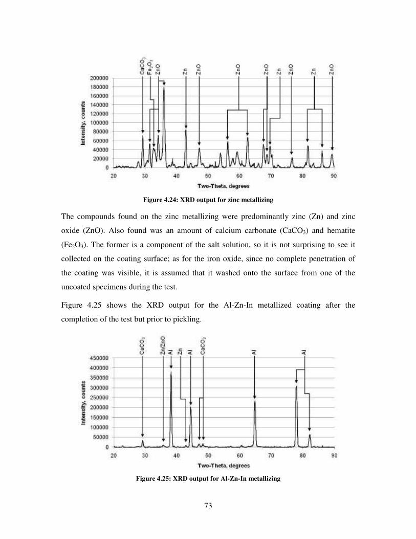
73

Figure 4.24: XRD output for zinc metallizing

The compounds found on the zinc metallizing were predominantly zinc (Zn) and zinc

oxide (ZnO). Also found was an amount of calcium carbonate (CaCO3) and hematite

(Fe2O3). The former is a component of the salt solution, so it is not surprising to see it

collected on the coating surface; as for the iron oxide, since no complete penetration of

the coating was visible, it is assumed that it washed onto the surface from one of the

uncoated specimens during the test.

Figure 4.25 shows the XRD output for the Al-Zn-In metallized coating after the

completion of the test but prior to pickling.

Figure 4.25: XRD output for Al-Zn-In metallizing

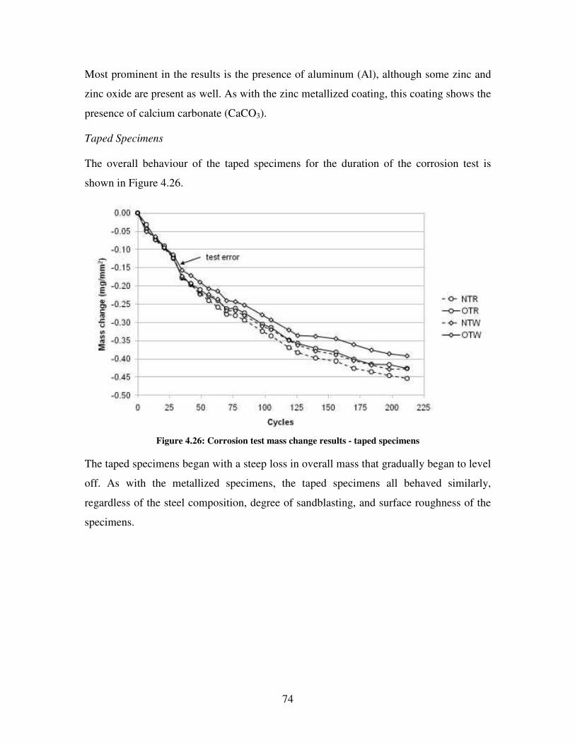
74

Most prominent in the results is the presence of aluminum (Al), although some zinc and

zinc oxide are present as well. As with the zinc metallized coating, this coating shows the

presence of calcium carbonate (CaCO3).

Taped Specimens

The overall behaviour of the taped specimens for the duration of the corrosion test is

shown in Figure 4.26.

Figure 4.26: Corrosion test mass change results - taped specimens

The taped specimens began with a steep loss in overall mass that gradually began to level

off. As with the metallized specimens, the taped specimens all behaved similarly,

regardless of the steel composition, degree of sandblasting, and surface roughness of the

specimens.

75

Figure 4.27 shows two examples of taped specimens prior to the start of the test.

Figure 4.27: NTR1 (left) and OTR1 (right), prior to start of test

Figure 4.28 shows the same specimens after they had been removed from the corrosion

chamber after 212 cycles.

Figure 4.28: NTR1 (left) and OTR1 (right), after end of test

As can be seen from Figure 4.28, little appears to have happened to most of the taped

specimens during the corrosion test. There are some exceptions: on specimen NTR1, a

blister had formed in the right-hand side of the tape. Figure 4.29 was taken after the

specimen had been sectioned and the PVC layer had been cut and removed from the zinc

tape with a scalpel.

76

Figure 4.29: Specimen NTR1, after sectioning and PVC layer removal

As can be seen from this figure, a significant amount of powdery white corrosion

product, thought to be zinc oxide (ZnO), had collected under the PVC coating.

The source of the mass loss is difficult to determine. As mentioned in Section 3, the tape

is a layer of pure zinc covered with a layer of PVC. For an oxidation reaction to occur,

the salt solution has to penetrate the layer; for mass loss to occur, the reaction products

have to escape the PVC layer again. However, most of the tape specimens do not appear

to have experience significant amounts of corrosion. Figure 4.30 shows another taped

new steel specimen with its PVC layer removed; very little corrosion product is visible.

Figure 4.30: Specimen NTR4 with PVC cover removed

77

The zinc layer in the specimen in Figure 4.30 is still shiny; when the zinc layer corrodes,

it becomes darker and duller. It is possible that some part of the mass loss is due to the

degradation of the PVC topcoat of the tape.

Figure 4.31 is a photomicrograph of a section taken from a tape-coated new steel

specimen.

Figure 4.31: Photomicrograph of NTR5 section

The PVC coating is not visible because it had peeled back during the sanding process. No

locations were found where the corrosion had penetrated the zinc layer.

Figure 4.32 is a photomicrograph of a taped new steel specimen which was subject to salt

solution penetration; the corrosion product forms little bumps on the zinc which are

visible through the PVC layer.

200 �m

Zinc metallizing

Base metal

Adhesive layer

78

Figure 4.32: Photomicrograph of NTR5 surface

Figure 4.33 shows the XRD results for a taped specimen after the PVC layer was

removed with a scalpel. It was possible to visually ascertain that the PVC coating had

protected the zinc layer since the zinc was still bright and little corrosion product was

visible.

Figure 4.33: XRD results for zinc tape with PVC layer removed

The only compounds found on the zinc tape specimen were zinc and, to a much smaller

degree, zinc oxide. This is consistent with what was expected for this specimen.

200 �m

79

4.2.4 Supplementary Tests

Calibration Test

Additional uncoated specimens were fabricated and placed in the corrosion tester to

measure more precisely the section loss to corrosion that occurs over time. The reason for

this was to estimate how a cycle or series of cycles in the corrosion tester related to a

given period of corrosion in the real world. A total of twelve plates of the same type of

steel as the “new steel” were introduced into the corrosion tester, with three being

removed, pickled and weighed every two weeks. These specimens were relatively thin

(approximately 3.6 mm thick on average) and had a large surface area. Figure 4.34 is a

chart with the specimen corrosion penetration plotted alongside the corrosion penetration

curve (± 1 standard deviation) of Equation 2.3.

Figure 4.34: Steel plate section loss comparison

Using the method of least squares to match the section loss of the specimens with the

corrosion penetration curve for weathering steel in marine environment (because of the

additional environmental factors required for the other corrosion rates, only marine

corrosion rate was used to calculate the equivalent test duration), it can be estimated that

a single cycle is equivalent to approximately 70 days; as such, the uncoated specimens

were tested for the equivalent of 15 years, and the coated specimens were tested for the

equivalent of 40 years. However, it must also be noted that the section loss on the plate

specimens shown in Figure 4.34 was considerably smaller than that found on the

uncoated specimens exposed for a similar period. Using the average thickness loss in

Table 4.7 and the corrosion equation with the values for the marine corrosion rate, it

80

would appear that the specimens were in the corrosion machine for the equivalent of 120

years. This disparity is inexplicable.

Epoxy Test

Four epoxy blanks were also introduced into the corrosion machine in order to test their

behaviour under the test conditions. The four blanks were cast in the same forms but had

varying masses, so that their surface area was largely the same but their volumes and

masses varied substantially. Table 4.8 contains the masses of the blanks at the start of the

test.

Table 4.8: Blank masses

Blank # Mass (g)

1 121.53

2 92.23

3 83.75

4 47.95

The results of the test are shown in Figure 4.35 and Figure 4.36.

Figure 4.35: Mass loss over time for blank specimens

81

Figure 4.36: Percentage mass loss over time for blank specimens

Over the course of the first 20 cycles the epoxy blanks increased in mass; after this, the

rate of mass gain either slowed or, in the case of the smallest, thinnest specimen, reversed

into mass loss. In any case, this test clearly indicates that the mass loss in the taped and

metallized specimens is not a result of mass loss on the part of the epoxy.

82

CHAPTER 5: STRUCTURAL ANALYSIS OF CORRODING BRIDGE GIRDERS

5.1 Introduction

In order to assess the reliability of the corroding highway structures, it was necessary to

create analytical models that take into account the following four factors:

1. the capacity of the structure;

2. the loading the structure must sustain;

3. the effects of progressive corrosion on the structural capacity; and

4. the statistical variations associated with factors 1 – 3.

Programs that consider these structural and statistical issues were written in Microsoft

Excel, with Visual Basic for Applications (VBA) employed where appropriate. The

following two program types were created:

1. Deterministic analysis programs to perform deterministic structural design checks

of the structures. The output, in each case, is a table of deterministic design ratios

(strength/resistance) for various limit states and locations along the bridge span.

2. Probabilistic or reliability analysis programs to determine the probability of

failure associated with the various limit states and locations along the bridge span

versus the number of years in service.

Variants of these programs were created for analyzing the following structure types:

1. simply supported box girder bridges;

2. simply supported I-girder bridges; and

3. two-span continuous box girder bridges.

5.2 Deterministic Analysis Programs

5.2.1 General

All of the structural analysis programs written for the current study follow the procedures

and principles of the [CAN/CSA-S6-06] Canadian Highway Bridge Design Code.

Specifically, they include the ultimate limit state calculations outlined in Section 10 of

83

this code; likewise, the loading, load factors, and load distribution are taken from

Sections 3 and 5 of [CAN/CSA-S6-06].

Limit State Equations

A total of five failure modes are considered at several points along the span; each failure

mode or “limit state” is identified and quantified by [CAN/CSA-S6-06], as follows:

1. shear ( 0.1≤rf VV );

2. moment ( 0.1≤rf MM );

3. shear + moment ( 0.1455.0727.0 <+ rfrf VVMM );

4. bearing ( 0.1≤rf BB ); and

5. web breathing or fatigue effects in the web ( ygFwh 3150≤ );

where V, M, and B are shear, moment, and bearing, respectively. The subscript f denotes

the factored load effect and the subscript r denotes the resistance of the girder. Also, h is

the web height, w is the web thickness, and Fyg is the yield stress of the girder.

Failure modes 1 to 4 are considered to be ultimate limit states, meaning that their

violation would result in structural failure. Mode 5 may be considered as a serviceability

limit state, since its violation is not expected to result in immediate structural failure.

For the calculation of shear resistance, the following formula is applied:

swsr FAV φ= where tcrs FFF += and: (5.1)

when ygv Fkwh 502≤ , ygcr FF 577.0= and 0=tF

when ygvygv FkwhFk 621502 ≤< , wh

FkF

ygv

cr

290= and

[ ] ( )[ ] 2121866.05.0−

+−= haFFF crygt

when ygv Fkwh 621> , ( )2

180000

wh

kF v

cr = and

84

[ ] ( )[ ] 2121866.05.0−

+−= haFFF crygt

where ( )2

34.54

hakv += when 1<ha

and ( )2

434.5

hakv += when 1≥ha

In Equation 5.1, sφ is the resistance factor for steel, Aw is the area of the web, and Fs is

the shear strength at the ultimate limit state; a is the horizontal spacing between vertical

web stiffeners, Ft is tension field component of post-buckling stress, Fcr is the shear

buckling stress, and kv is the shear buckling coefficient. For the calculation of positive

moment resistance of the composite box girder bridge, the girder is assumed to behave

plastically. Figure 5.1 to Figure 5.3 show the assumed distribution of stresses across the

girder depth for various neutral axis locations.

Figure 5.1: Plastic section analysis - neutral axis in the slab

85

Figure 5.2: Plastic section analysis - neutral axis in upper web

Figure 5.3: Plastic section analysis - neutral axis in lower web

In Figure 5.1 to Figure 5.3, the tension in the lower part of the steel girder (Ts) in each

case is counterbalanced by the compression in the top part of the steel girder (Cs), the

concrete slab (Cc), and the reinforcement (Cr). The moment resistance is a function of

these forces and the eccentricities between them (es, ec, and er). f’c is the assumed

nominal concrete compressive strength, fyr is the assumed nominal yield strength of the

rebar, and Fyg is the assumed nominal yield strength of the weathering steel girder.

When the neutral axis is in the slab (Figure 5.1), the moment resistance is:

rrccr eCeCM += (5.2)

When the neutral axis is in the web (Figure 5.2), but less than ygFw850 below the top

of the web, the moment resistance is:

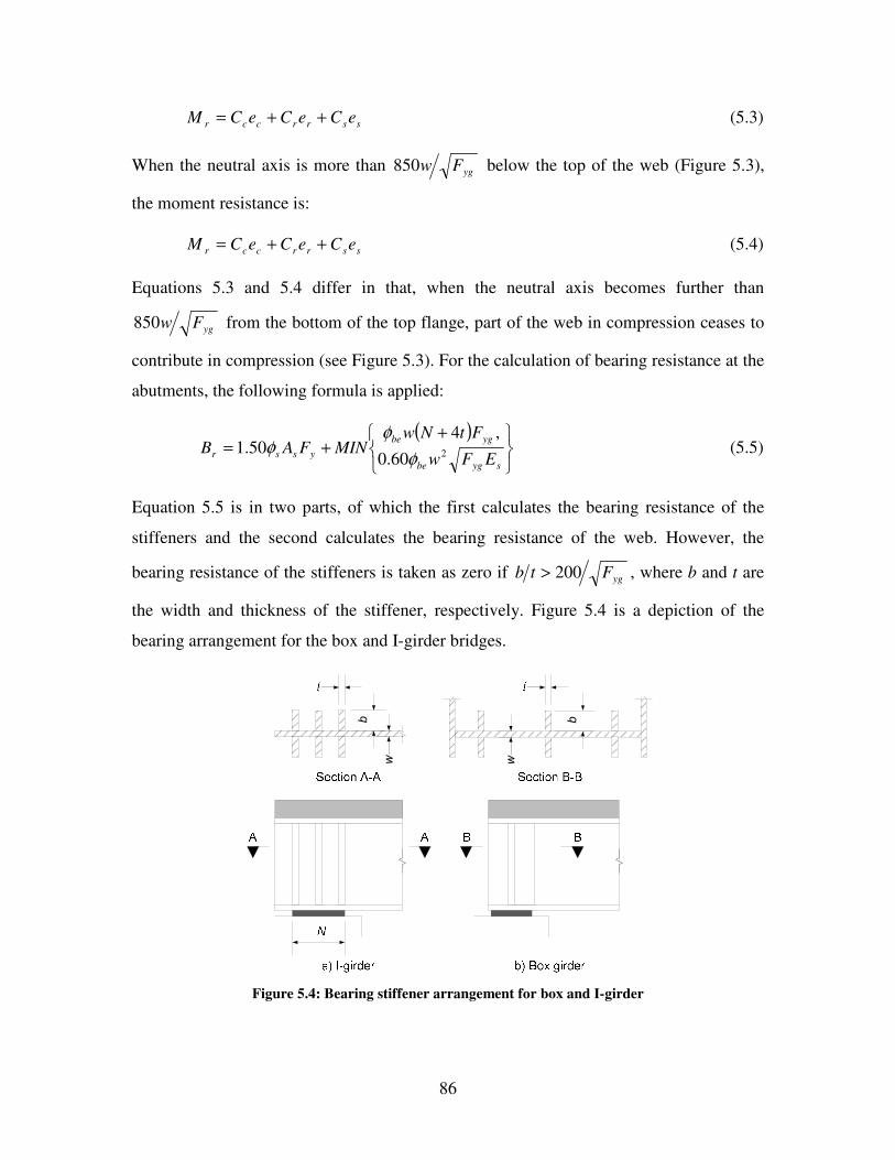
86

ssrrccr eCeCeCM ++= (5.3)

When the neutral axis is more than ygFw850 below the top of the web (Figure 5.3),

the moment resistance is:

ssrrccr eCeCeCM ++= (5.4)

Equations 5.3 and 5.4 differ in that, when the neutral axis becomes further than

ygFw850 from the bottom of the top flange, part of the web in compression ceases to

contribute in compression (see Figure 5.3). For the calculation of bearing resistance at the

abutments, the following formula is applied:

( )�

�� +

+=sygbe

ygbeyssr EFw

FtNwMINFAB 260.0

,450.1 φ

φφ (5.5)

Equation 5.5 is in two parts, of which the first calculates the bearing resistance of the

stiffeners and the second calculates the bearing resistance of the web. However, the

bearing resistance of the stiffeners is taken as zero if ygFtb 200> , where b and t are

the width and thickness of the stiffener, respectively. Figure 5.4 is a depiction of the

bearing arrangement for the box and I-girder bridges.

�

� �

�

Figure 5.4: Bearing stiffener arrangement for box and I-girder

87

In Equations 5.1 – 5.5, the φ factors are material resistance factors for the concrete ( cφ ),

rebar ( rφ ), and steel ( sφ ). The factor beφ is a special resistance factor for beam end web

bearing. The values for the factors are contained in Table 5.2.

Table 5.1: Resistance factors [CAN/CSA-S6-06]

Element Factor

Structural steel, sφ 0.95

Reinforcing steel, rφ 0.90

Concrete, cφ 0.75

Bearing (at abutment), beφ 0.75

The resistance factors are applied at the ultimate limit state to account for variability of

material properties and dimensions, as well as quality of work, type of failure, and the

uncertainties associated with these parameters [CAN/CSA-S6-06]. These factors are only

applied in the deterministic programs; in the probabilistic programs, they are all set to 1.0

and statistical “bias factors” are used to modify the resistances.

Loading Analysis

Only dead and live (traffic) loads are considered in the current analysis, since these

typically dominate the design of short- and medium-span bridges. Two types of dead load

are taken into account. The superimposed dead load refers to the sidewalk and wearing

surface, while the dead load itself refers to the slab and steel girder self weight.

The slab, wearing surface, sidewalks and barriers were treated as uniformly distributed

loads (UDL); their gravity loads per metre were summed and divided by the number of

girders. The self-weight of the girder was likewise treated as a UDL.

The unit weights assumed to calculate the dead loads are given in Table 5.2.

88

Table 5.2: Unit weights of structural components [CAN/CSA-S6-06]

Component Weight

Bituminous wearing surface 23.5 kN/m3

Concrete 24.0 kN/m3

Steel 77.0 kN/m3

As prescribed in [CAN/CSA-S6-06], the live load (LL) is taken as the greater of a five-

axle truck load and a truck-plus-lane load, as shown in Figure 5.5 and Figure 5.6.

Figure 5.5: CL-625 ONT axle load

Figure 5.6: CL-625 ONT lane load

Factors

Table 5.3 shows the factors applied for ultimate limit state verification under the dead

plus live load combination (load combination ULS1 [CAN/CSA-S6-06]). These factors

assume that the dead load will always be detrimental. In the probabilistic programs, these

factors are set to a value of 1.0 and their effect is accounted for statistically.

89

Table 5.3: Load factors [CAN/CSA-S6-06]

Load type Factor

Live load (traffic) 1.70

Superimposed dead load (wearing surface) 1.50

Cast-in-place dead load (concrete deck) 1.20

Manufactured dead load (steel girder) 1.10

Along with the live load factor, the live (traffic) load effects are multiplied by an

additional factor, which takes into account the dynamic component of the live load,

called the dynamic load allowance (DLA). The value of the DLA varies with the number

of axles of the CL-W truck used in the analysis. Axle numbers are as per the drawing in

Figure 5.5. The DLA values are contained in Table 5.4.

Table 5.4: Dynamic load allowances [CAN/CSA-S6-06]

Axle(s) used DLA

Only one axle 0.40

Any two axles, or axles 1 to 3 0.30

Any three axles, except for axles 1 to 3, or more than three axles 0.25

In the statistical programs, the axle load (but not the lane load) is multiplied by (1 +

DLA). In the probabilistic programs, the DLA is treated as a statistical variable.

In certain cases, there is also a modification factor for multi-lane loading (by which the

live load effects may be multiplied), to take into account the likelihood of having more

than one lane loaded at any given time. These values are contained in Table 5.5.

90

Table 5.5: Modification factor for multi-lane loading [CAN/CSA-S6-06]

Number of loaded design lanes Factor

1 1.00

2 0.90

3 0.80

4 0.70

For multi-girder bridges, there is also a live load amplification factor (LLAF) that may be

applied to the live load to account for the transverse sharing of these loads between the

girders. The LLAF for the moment on a single-span bridge is:

05.1

100

≥

��

���

�=

fm C

F

SNF

µ (5.6)

Where Fm is the amplification factor to account for the transverse variation in the

maximum longitudinal moment intensity, as compared to the average longitudinal

moment intensity, S is the centre-to-centre girder spacing, and N is the number of girders.

The values for F, the width dimension that characterizes the load distribution for the

bridge, and Cf, the correction factor used to adjust the F value for longitudinal moment

and longitudinal vertical shear, are contained in Table 5.6.

91

Table 5.6: F and Cf values for moment [CAN/CSA-S6-06]

Box girder I girder

Lanes F Cf F Cf

2 8.5 – 0.3� 16 – 2� 6.80 – (3/L)*

7.20 – (14/L)** 10 – (25/L)

3 11.5 – 0.5� 16 – 2� 8.70 – (4/L)*

9.60 – (21/L)** 10 – (25/L)

4 14.5 – 0.7� 16 – 2� 10.00 – (5/L)*

11.20 – (22/L)** 10 – (25/L)

* For external girder ** For internal girder

The values in Table 5.6 assume a bridge span of at least 10 m. The lane width

modification factor, �, is calculated with the following equation:

0.16.0

3.3≤

−= eWµ (5.7)

where We is the width of the design lane. For the box girders, the � parameter is taken as:

5.0

���

�

���

���

���

�=xy

x

DD

LBπβ (5.8)

where B and L are the bridge width and length respectively; Dx is the total bending

stiffness (equal to the modulus of elasticity times the moment of inertia) of the bridge

cross-section divided by the width of the bridge, and Dxy is the total torsional stiffness

(equal to the shear modulus times the torsional inertia) of the bridge cross-section divided

by the width of the bridge. The LLAF for the shear is:

F

SNFv = (5.9)

where the S and N values are the same as above. The F value is tabulated in [CAN/CSA-

S6-06]; Table 5.7 summarizes the relevant values for box and I-girders.

92

Table 5.7: F values for shear [CAN/CSA-S6-06]

Lanes Box girder I-girder

2 7.20 6.10

3 9.60 8.20

4 11.20 9.50

The procedure described above for the application of the LLAF is a simplified, and

conservative, approach; other, more laborious means of calculating this factor exist, such

as by finite element modelling. For its valid application, certain requirements are laid out

in [CAN/CSA-S6-06]. These requirements are listed in Table 5.8.

Table 5.8: LLAF requirements

Box girder (multispine) bridges I-girder bridges

• bridge has constant width

• support conditions are closely equivalent to line support at the ends of the bridge

• overhang is not more than 1.80 m and does not exceed the spacing of the two outermost adjacent webs

• at least two longitudinal girders of approximately equal flexural rigidity and spacing

• each spine has only two webs

• number of lanes is larger than or equal to the number of spines

• bridge’s length is greater that its width

• bridge has constant width

• support conditions are closely equivalent to line support at the ends of the bridge

• overhang is not more than 1.80 m and does not exceed 60% of the spacing between the girders

• at least three girders of approximately equal flexural rigidity and spacing

5.2.2 Simply Supported Structures

In the deterministic and probabilistic analysis programs for simply supported structures,

the span of the structure is divided into ten sections, with the relevant limit states being

calculated at the beginning and end of each section (eleven locations along the span).

93

Also, up to seven different sections can be specified for the span; each of these sections

can have its own length, girder geometry, corrosion rate, and corrosion scenario.

To calculate the live (truck) loading, the axle loads are moved along the length of the

bridge (at the specified axle spacing) at 1 m increments, and the maximum shear and

moment resultants at each of the eleven locations along the span are kept for the analysis

procedure. Both dead and live load effects are calculated with closed form equations in

the VBA program as a preliminary stage to the bridge analysis.

5.2.3 Two-Span Continuous Structures

The program for analyzing two-span continuous bridges is similar to the single-span

program in many respects; however, the two-span program is necessarily more complex.

Because a two-span continuous structure is statically indeterminate, it was necessary to

build a finite element model to perform the analysis. Due to the regularity of the problem

and in order to more easily integrate the structural analysis into a single program with the

resistance verification, a finite element code was written in VBA for this purpose.

The finite element model is composed of beam elements, which have four degrees of

freedom each, representing the vertical displacement, q1 and q3, and the rotation, q2 and

q4, of the two nodes. A typical element is depicted in Figure 5.7.

Figure 5.7: Free body diagram of beam element

The two-span continuous model is composed of two spans of ten elements each, for a

total of twenty elements and twenty-one nodes. As such, the girder of each span can be

broken up into segments with different cross-sectional geometries. It is not necessary that

the two spans are identical. The element stiffness matrix is as follows:

q1 q3

q4 e

�e

q2

94

����

�

�

����

�

�

−−−−

−−

=

22

22

3

4626612612

2646612612

eeee

ee

eeee

ee

e

e EIk

����

��

����

��

� (5.10)

As with any finite element program, the individual element stiffness matrices are

combined into a global stiffness matrix and joined with the global force matrix to solve

for displacements and reactions.

Loading Analysis

The loading cases for a two-span continuous structure are the same as for a simply

supported structure. The live load due to the CL-625 ONT truck is again assumed; and

again, both the axle and lane variants of this loading are considered. However, for the

two-span continuous bridge the truck is moved across only eleven locations on each span,

and the centre of gravity of the truck is used to locate it.

Limit State Equations

Since the negative moment puts a significant portion of the web into compression, the

structural resistance to negative moment is calculated using the elastic section modulus.

Furthermore, different sections are considered for different stages of loading: the load of

the girder plus the slab is compared against the resistance of the girder alone, while the

load of the girder, slab, wearing surface, and rails is compared against the resistance of

the composite section before creep, and the live load is compared against the resistance of

the composite section after creep. The purpose of this is to simulate the loads introduced

into the system at each stage of the construction sequence.

Three different limit states are considered with respect to moment: the stresses in the

reinforcement (1) and the top fibre of the top flange (2) must not exceed the yield stress,

and the bottom flange (3), which is in compression, must not buckle. Therefore, three

equations are required to verify the moment limit state:

For the bottom flange: ( ) crsflfsdfd FSMMSM φ≤++ ' (5.11)

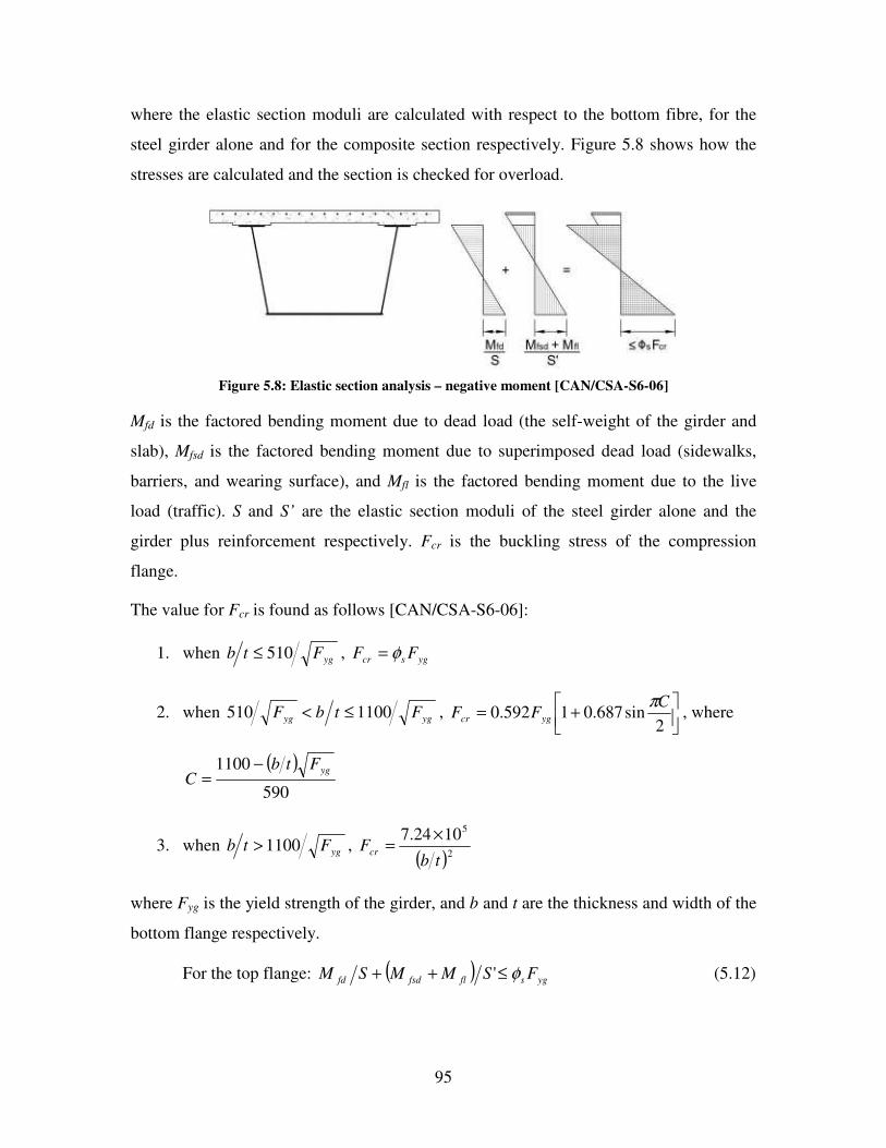
95

where the elastic section moduli are calculated with respect to the bottom fibre, for the

steel girder alone and for the composite section respectively. Figure 5.8 shows how the

stresses are calculated and the section is checked for overload.

Figure 5.8: Elastic section analysis – negative moment [CAN/CSA-S6-06]

Mfd is the factored bending moment due to dead load (the self-weight of the girder and

slab), Mfsd is the factored bending moment due to superimposed dead load (sidewalks,

barriers, and wearing surface), and Mfl is the factored bending moment due to the live

load (traffic). S and S’ are the elastic section moduli of the steel girder alone and the

girder plus reinforcement respectively. Fcr is the buckling stress of the compression

flange.

The value for Fcr is found as follows [CAN/CSA-S6-06]:

1. when ygFtb 510≤ , ygscr FF φ=

2. when ygyg FtbF 1100510 ≤< , ��

���

� +=2

sin687.01592.0C

FF ygcr

π, where

( )590

1100 ygFtbC

−=

3. when ygFtb 1100> , ( )2

51024.7tb

Fcr

×=

where Fyg is the yield strength of the girder, and b and t are the thickness and width of the

bottom flange respectively.

For the top flange: ( ) ygsflfsdfd FSMMSM φ≤++ ' (5.12)

96

where the elastic section moduli are calculated with respect to the top fibre of the steel

section, for the steel girder alone and for the composite section respectively.

For the top layer of reinforcement: ( ) yrrflfsd FSMM φ≤+ ' (5.13)

where the elastic section modulus is calculated with respect to the centroid of the top

layer of slab reinforcement for the composite section.

In [CAN/CSA-S6-06] a girder section is defined by its class, which is determined by the

width-to-thickness ratios of its component members. Class 1 and 2 sections are capable of

achieving the full plastic moment capacity; Class 3 sections only have elastic moment

capacity (as such, only the outermost fibre of the girder may undergo yield stress), while

Class 4 sections would experience local buckling below this applied moment level [Kulak

& Grondin 2006]. Due to the fact that the webs and bottom flanges of the box girder

section lose section as time progresses in the program, either one or both may become

Class 4 members. [CAN/CSA-S6-06] requires that either the web or the flange be a Class

3 member, but in the context of this research this requirement was thought to be overly

restrictive. In order to take into account the additional reduction in the resistance due to

member slenderness of the continuous box girder under negative moments, the box girder

section is treated as a stiffened plate girder: in the case where ygc Fwd 19002 > , the

negative moment resistance is multiplied by the following factor:

��

�

�

��

�

�−

+−

yg

c

wcf Fwd

AA19002

12003001

1 (5.14)

where dc is the depth of compression portion of web in flexure, w is the web thickness,

Acf is the area of the compression flange, and Aw is the area of the web.

For the calculation of bearing resistance at the midspan, the following formula is applied

[CAN/CSA-S6-06], which is similar to Equation 5.5 for end bearing:

( )�

�� +

+=sygbi

ygbiygssr EFw

FtNwMINFAB 245.1

,1050.1 φ

φφ (5.15)

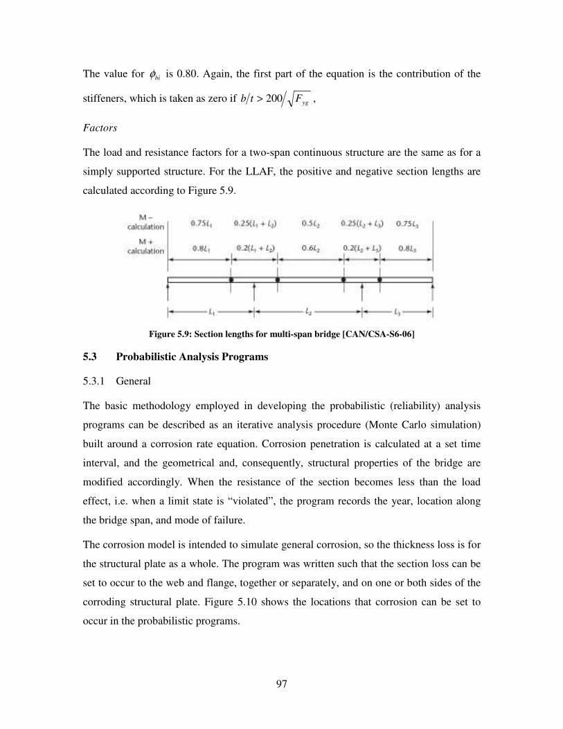
97

The value for biφ is 0.80. Again, the first part of the equation is the contribution of the

stiffeners, which is taken as zero if ygFtb 200> ,

Factors

The load and resistance factors for a two-span continuous structure are the same as for a

simply supported structure. For the LLAF, the positive and negative section lengths are

calculated according to Figure 5.9.

Figure 5.9: Section lengths for multi-span bridge [CAN/CSA-S6-06]

5.3 Probabilistic Analysis Programs

5.3.1 General

The basic methodology employed in developing the probabilistic (reliability) analysis

programs can be described as an iterative analysis procedure (Monte Carlo simulation)

built around a corrosion rate equation. Corrosion penetration is calculated at a set time

interval, and the geometrical and, consequently, structural properties of the bridge are

modified accordingly. When the resistance of the section becomes less than the load

effect, i.e. when a limit state is “violated”, the program records the year, location along

the bridge span, and mode of failure.

The corrosion model is intended to simulate general corrosion, so the thickness loss is for

the structural plate as a whole. The program was written such that the section loss can be

set to occur to the web and flange, together or separately, and on one or both sides of the

corroding structural plate. Figure 5.10 shows the locations that corrosion can be set to

occur in the probabilistic programs.

98

Figure 5.10: Assumed corrosion locations

The steel surfaces with a bold line in Figure 5.10 can be made subject to corrosion in the

programs. These surfaces include the exposed surfaces of the web and bottom flange of

the box girder, and both sides of the web and bottom flange of the I-girder. Note that, in

Chapter 6, a number of analyses are presented for the case of an I-girder with only the top

of the bottom flange corroding (rather than both the top and bottom), to simulate a

particular corrosion scenario that has been observed in some jurisdictions (including

Ontario) [Albrecht & Naeemi 1984, Albrecht et al. 1989].

The program is set to operate for a predetermined number of runs and stores the output of

each one. The program employs a basic Monte Carlo simulation algorithm to consider the

statistical variability in the various input parameters [Melchers 2002].

5.3.2 Simply Supported Structures

Figure 5.11 shows a flow chart of the operation of the probabilistic (reliability) analysis

program for the simply supported case.

99

��� ��������������������������� ����

��� �������� �������������� ��������

��� ����������������������������������� ��

���� �����

��� �������������������� !

"���#��$

%����

%����������������

�� ����������&���

"��

'�

"��

�����#��$"��

'�

%���

(������������������������

) ��#��$

'�

(������������ �������������������

(������������ ������������������

"��

Figure 5.11: Probabilistic program flowchart – simply supported structures

5.3.3 Two-Span Continuous Structures

The two-span continuous program is considerably more complex as the load effects are

dependent on the cross-section properties for this indeterminate structural system.

Likewise, it has a significantly longer run time. Because the cross section of the girder

diminishes with each passing increment of time, causing a redistribution of the loading, it

is necessary to analyze the structure anew at each time increment. Figure 5.12 shows the

probabilistic program flowchart for the two-span continuous structure analysis.

100

Figure 5.12: Probabilistic program flowchart – two-span continuous structures

101

5.3.4 Statistical Variables

For the probabilistic analysis, the uncertainties associated with various deterministic

model parameters can be considered by multiplying them by appropriate statistical

variables or “bias factors”. These parameters include the material strengths, calculated

resistances, and dead and live loads and effects. The assumed statistical distributions for

the corresponding bias factors are listed in Table 5.9.

Table 5.9: Statistical variables and assumed distributions

Bias Factor Input Parameter

Dist. Type Mean Std. Dev.

Compressive strength of concrete (f’c) Lognormal 0.805 0.150

Yield strength (Fyg) of girder Lognormal 1.101 0.092

Yield strength (Fyr) of rebar Lognormal 1.115 0.100

Moment resistance (Mr) factor Normal 1.098 0.096

Shear resistance (Vr) factor Normal 1.178 0.103

Manufactured components DL Normal 1.030 0.080

Cast-in-place components DL Normal 1.050 0.100

Superimposed DL Normal 1.030 0.300

LL analysis factor Normal 0.930 0.120

Dynamic factor (DLA) Normal 1.100 0.072

LL shear and moment factor Gumbel See Table 5.10

The source for all these values is [CAN/CSA-S6-00 Calibration], except for the values

for f’c and Fyr, which both come from [Cheung & Li 2002]

The values for the mean and standard deviation of the bias factors associated with the

concrete compressive strength, f’c and rebar yield strength, fyr were derived from

available test data in [Tabsh & Nowak 1991]. The values used are in the lower end of the

range of values found in relevant works; nevertheless, they were thought to be

appropriate due to the difficult nature of the work (i.e. bridge vs. normal construction),

102

the problems associated with placing concrete in certain conditions. The values for the

mean and standard deviation of the girder yield stress, Fyg, bias factor originate from the

work of Kennedy & Baker [1984] on the subject of resistance factors for steel highway

bridges. The factors for steel and concrete take into account three sources of error:

material, geometrical, and manufacturing/construction.

The factors modifying the dead load of the manufactured and cast-in-place structural

elements (the steel girder and concrete slab) were originally from the work done by

Nowak and Grouni for calibrating the Ontario Highway Bridge Design Code, which was

subsequently verified by other sources for [CAN/CSA-S6-06]. The factor modifying the

superimposed dead load, meaning the asphalt wearing surface, is based on field data

reported in [CAN/CSA-S6-00 Calibration].

The live load (LL) analysis factor is recommended by the Canadian Highway Bridge

Design Code Subcommittee on Analysis; the live load distribution methods of

[CAN/CSA-S6-06] are considered to have an intrinsic conservatism, and this factor is

required as a result. Two options are given, depending on the level of sophistication of

the analysis method.

The dynamic loading factor (DLA) is based on field measurements, performed in

Ontario, of a variety of bridges. Trucks requiring special permits were not distinguished

since a lower rate of travel is required, thus bringing their contribution in line with those

of the regular traffic.

The additional live load (LL) shear and moment factors (see Table 5.10) are also taken

from data specific to Ontario, where a survey of trucks was performed in 1995. Only

normal traffic, as opposed to traffic operating with a special permit, was considered.

Trucks with an average axle weight � 4.0 T were screened out, but the total number of

trucks (N = 13391) was used as the sample size. Models of a number of these vehicles

were driven over bridges of varying lengths in order to determine their shear and moment

resultants. These data were combined to generate load-effect histograms.

In [CAN/CSA-S6-00 Calibration], a Gumbel distribution is used to represent the extreme

annual statistics for different load effects (i.e. shear, moment) and bridge spans /

configurations. A methodology for doing this is presented in this reference, along with

103

the resulting load effect extreme value distributions for a Class A highway over a one

year time period. The methodology can be summarized as follows: Since the actual

distribution of load effects is generally not perfectly normal, a representative normal

distribution (RND) had to first be established; this was done by focussing on the tail end

of the distribution, which was assumed to have properties similar to that of the RND tail.

First, a load effect sample was generated, by simulating the passage of a limited number

of actual measured trucks (~10,000) over a load effect influence line for a particular

bridge span / configuration. Next, two assumptions were made, regarding the resulting

sample: first, that the highest value in the sample load effect distribution is an extreme

value in the Gumbel distribution for that sample size, and second, that this highest value

is three standard deviations above the mean in the Gumbel distribution. If the highest

value was significantly larger than the next highest value, the former was used in order to

prevent the distribution from being affected by suspect measurements. As such, values

for mean and standard deviation of the RND can be derived, and from them the Gumbel

distribution for the extreme load effect events corresponding with a certain period of time

(for a given traffic volume). By following the same method as that presented in

[CAN/CSA-S6-00 Calibration] herein, it was possible to develop bias factor mean and

variance values for any time period / highway class.

In [CAN/CSA-S6-06], four different classes of highway (A to D) are defined by their

average daily truck traffic (ADTT) rates (see Table 5.10).

Table 5.10: Highway classes [CAN/CSA-S6-06]

Highway class ADTT (per lane)

A 1000 – 4000

B 250 – 1000

C 50 – 250

D < 50

Traffic rate variations are only considered for the 40 m simply supported bridge analyzed

herein. The bias factor values still change, however, for different spans / configurations,

since the influence lines are different. Table 5.11 contains these values. The means and

104

coefficients of variation in this table reflect the different load effect sample distributions

for shear (V) and moment (M). The extreme value distributions presuppose a certain time

interval, which is likewise provided in Table 5.11.

Table 5.11: LL shear and moment bias factors (based on 10 year extreme event statistics)

Highway class Structure type Span (m) Interval (yr) Mean CoV

A Simply supported 40 10

1.503 (V)

1.461 (M)

0.033 (V)

0.033 (M)

B Simply supported 40 10

1.446 (V)

1.405 (M)

0.036 (V)

0.036 (M)

C Simply supported 40 10

1.386 (V)

1.346 (M)

0.040 (V)

0.040 (M)

D Simply supported 40 10

1.312 (V)

1.273 (M)

0.045 (V)

0.045 (M)

A Simply supported 30 10

1.541 (V)

1.542 (M)

0.032 (V)

0.032 (M)

A Simply supported 35 10

1.543 (V)

1.501 (M)

0.032 (V)

0.033 (M)

C Two-span continuous 40 8

1.097 (V)

1.290 (M)

0.040 (V)

0.042 (M)

Along with the statistical variables listed in Table 5.9, two additional parameters are

statistically varied in the reliability program, namely the A and B factors of the corrosion

penetration equation (Equation 2.3). The means and standard deviations of these factors

for the rural, marine, and urban environments are given in Table 5.12.

Kayser [1988] calculated numerical values for the A and B variables using experimentally

obtained corrosion data for rural, industrial, and marine environments compiled in

[Albrecht & Naeemi 1984]. These results were assembled in order to come up with

values for each corrosion rate, as well as their statistical distributions.

105

Table 5.12: Corrosion rate parameters

Environment Variable Mean CoV

A 33.3 0.34 Rural

B 0.498 0.09

A 40.2 0.22 Marine

B 0.557 0.10

A 50.7 0.30 Urban

B 0.567 0.37

The above data are based upon corrosion of weathering steel specimens in the United

States, the United Kingdom, and Germany. Noteworthy is the relatively high coefficient

of variation of the urban corrosion rate’s B variable, because as the power variable, it

introduces a high degree of variability into the corrosion penetration results. A lognormal

distribution is assumed for each of these statistical variables.

5.3.5 Statistical Programming

Monte Carlo Simulation

Monte Carlo simulation (MCS) enables the statistical analysis of a complex structural

system by repeating the loading and resistance calculations until a statistically significant

number of “trials” has been collected. Rather than solving a single, highly complex

equation, which would take into account the interaction of a number of statistical

variables, Monte Carlo simulation enables the calculation to be performed numerous

times with randomly selected values (generated anew each time) for the various statistical

variables. The probability of failure is then calculated from the following equation:

( )( )

tf N

zGnp

0≤= 5.15

where Nt is the total number of trials, and ( )( )0≤zGn is the total number of trials for

which the limit states were violated (ref. Equations 2.8 to 2.10).

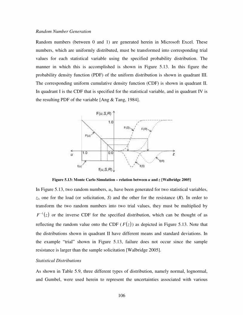
106

Random Number Generation

Random numbers (between 0 and 1) are generated herein in Microsoft Excel. These

numbers, which are uniformly distributed, must be transformed into corresponding trial

values for each statistical variable using the specified probability distribution. The

manner in which this is accomplished is shown in Figure 5.13. In this figure the

probability density function (PDF) of the uniform distribution is shown in quadrant III.

The corresponding uniform cumulative density function (CDF) is shown in quadrant II.

In quadrant I is the CDF that is specified for the statistical variable, and in quadrant IV is

the resulting PDF of the variable [Ang & Tang, 1984].

Figure 5.13: Monte Carlo Simulation – relation between u and z [Walbridge 2005]

In Figure 5.13, two random numbers, ui, have been generated for two statistical variables,

zi, one for the load (or solicitation, S) and the other for the resistance (R). In order to

transform the two random numbers into two trial values, they must be multiplied by

( )zF 1− or the inverse CDF for the specified distribution, which can be thought of as

reflecting the random value onto the CDF ( ( )zF ) as depicted in Figure 5.13. Note that

the distributions shown in quadrant II have different means and standard deviations. In

the example “trial” shown in Figure 5.13, failure does not occur since the sample

resistance is larger than the sample solicitation [Walbridge 2005].

Statistical Distributions

As shown in Table 5.9, three different types of distribution, namely normal, lognormal,

and Gumbel, were used herein to represent the uncertainties associated with various

107

deterministic model parameters. The equations for the PDF and CDF for each distribution

type are given in Table 5.12.

Table 5.12: Statistical distribution equations [Melchers 2002]

Distribution Equation

Normal

PDF: ( )( ) �

�

�

�

��

�

�

���

����

� −−=

2

21 21

exp2

1

X

X

XX

xxf

σµ

σπ, ∞≤≤∞− x

CDF: ( ) ( )( )

dvexFxXPs v

X � ∞−

−==≤

2

21

2121

π, ∞≤≤∞− x

where ( ) xxxs σµ−= . There is no simple expression for ( )xFX .

Lognormal

PDF: ( )( ) �

��

�

���

���

���

� −−=2

21

ln21

exp2

1ε

λπ

x

xexf x , ∞≤≤ x0

CDF: ( ) ( ) ��

���

� −Φ== � ∞− ελx

duufxFx

xxln

(no explicit form)

where ( ) xxE lnln µλ == and ( ) 2ln

2 lnvar xx σε ==

Gumbel

PDF: ( ) ( ) ( )[ ]uyY euyyf −−−−−= ααα exp , ∞≤≤∞− y

CDF: ( ) ( )[ ]uyY eyF −−−= αexp , ∞≤≤∞− y

where 2

22

6 Yσπα = and

αµ 1396.1−= Yu

The normal distribution is a basic distribution that can be used to describe any variable

that groups about a mean value, e.g., the standard bell curve. This distribution is used for

most of the load factors. Figure 5.14 shows an example of normal, lognormal, and

Gumbel distribution PDFs. Note that the mean and standard deviation of each of the

PDFs shown in Figure 5.14 are 1.0 and 0.5 respectively.

108

Figure 5.14: Normal, Lognormal, and Gumbel distribution PDFs

In a lognormal distribution, the natural logarithm of a randomly generated value between

0 and 1 has a normal distribution, rather than the number itself. It is a single-tailed

distribution; this is why it is commonly used for material strengths and corrosion rates

(and other parameters for which a negative trial value is not admissible).

Gumbel distribution is an extreme value distribution. It is commonly used to model the

distribution of the extreme values from a number of samples. Like the normal distribution

PDF, negative values are possible, but values significantly larger than the mean are more

likely.

5.3.6 Reliability

A procedure for determining an appropriate target reliability index, �target, for a given

bridge is laid out in Chapter 14 of [CAN/CSA-S6-06]. The categories of the structural

system (S), the element (E) under consideration, and the inspection level (INSP) of the

structure are considered in deciding the �target value.

System Behaviour

If the structural system under consideration would totally collapse as a result of failure of

the element under consideration, the system category is S1. If element failure probably

will not result in total collapse, the system category is S2, while if it will lead to local

failure only, the system category is S3.

5.00.1

==

x

x

σ

109

Element Behaviour

If the element under consideration fails suddenly, with little or no warning, the element is

classified as E1. If the failure is sudden and not preceded by a warning, but retains some

post-failure capacity, then the element category is E2. If the element under consideration

fails gradually, with warning of its impending failure, it is E3.

Inspection Level

If the element under consideration is not inspectable, it belongs to the INSP1 category. If,

however, the inspection is performed to the satisfaction of the evaluator and the results of

the inspection are available to him, it is INSP2. Finally, if the evaluator has directed the

inspection of every critical component and evaluation calculations, it is INSP3.

Category Values

The values for the categories described above are provided in Table 5.13.

Table 5.13: Target reliability index, �target, for normal traffic [CAN/CSA-S6-06]

Inspection level System behaviour category

Element behaviour category INSP1 INSP2 INSP3

S1

E1

E2

E3

4.00

3.75

3.50

3.75

3.50

3.25

3.75

3.25

3.00

S2

E1

E2

E3

3.75

3.50

3.25

3.50

3.25

3.00

3.50

3.00

2.75

S3

E1

E2

E3

3.50

3.25

3.00

3.25

3.00

2.75

3.25

2.75

2.50

For a highway structure like the ones being considered herein, �target, ranges from 2.75 to

3.25. The structural system category for bridges with multiple girders is S2, the elements

are in the E3 category, and the inspection level can vary according to the means of the

owner and the apparent condition of the structure.

110

CHAPTER 6: STRUCTURAL ANALYSIS RESULTS AND INTERPRETATION

In this chapter, the deterministic and reliability models developed in Chapter 5 are used

to: 1) examine the decline in the structural performance over time due to corrosion for

different structure types, 2) perform sensitivity studies to determine the significance of

various parameters on the structural performance, and 3) estimate the remaining service

lives of two existing structures for which inspection results have been made available by

MTO. Steps 1) and 2) are performed on hypothetical structures, designed using the

deterministic models from Chapter 5, as explained in the following section.

6.1 Bridge Designs

In order to examine the effects of various parameters on the performance of different

structure types, it was necessary to first design a number of hypothetical weathering steel

highway bridges with the key structural parameters varied within suitable ranges. The

parameters that are the focus of this study are summarized as follows:

1. Corrosion Scenario. For the box and I-girder structures, both corrosion to the web

and flange, and to the flange-only, are examined. For the I-girder structures,

corrosion to the top of the bottom flange-only is considered as well.

2. Highway Class. Bridges with traffic volumes matching the maximums of those of

Highway class A – D (see Table 5.10) are examined.

3. Girder Strength. Bridges with three different girder yield strengths (300, 350, and

480 MPa) are examined.

4. Bridge Span. Bridges with spans of 30, 35, and 40 m are examined.

5. Number of Lanes. Two- and four-lane bridges are examined herein.

Of these five parameters, numbers 3, 4, and 5 each require a new bridge design. Table 6.1

contains a list of the resulting bridge designs and their designations.

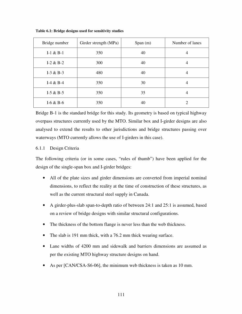
111

Table 6.1: Bridge designs used for sensitivity studies

Bridge number Girder strength (MPa) Span (m) Number of lanes

I-1 & B-1 350 40 4

I-2 & B-2 300 40 4

I-3 & B-3 480 40 4

I-4 & B-4 350 30 4

I-5 & B-5 350 35 4

I-6 & B-6 350 40 2

Bridge B-1 is the standard bridge for this study. Its geometry is based on typical highway

overpass structures currently used by the MTO. Similar box and I-girder designs are also

analysed to extend the results to other jurisdictions and bridge structures passing over

waterways (MTO currently allows the use of I-girders in this case).

6.1.1 Design Criteria

The following criteria (or in some cases, “rules of thumb”) have been applied for the

design of the single-span box and I-girder bridges:

• All of the plate sizes and girder dimensions are converted from imperial nominal

dimensions, to reflect the reality at the time of construction of these structures, as

well as the current structural steel supply in Canada.

• A girder-plus-slab span-to-depth ratio of between 24:1 and 25:1 is assumed, based

on a review of bridge designs with similar structural configurations.

• The thickness of the bottom flange is never less than the web thickness.

• The slab is 191 mm thick, with a 76.2 mm thick wearing surface.

• Lane widths of 4200 mm and sidewalk and barriers dimensions are assumed as

per the existing MTO highway structure designs on hand.

• As per [CAN/CSA-S6-06], the minimum web thickness is taken as 10 mm.

112

• As per [CAN/CSA-S6-06], the inclination of the web plates for box girders is not

allowed to exceed 1 horizontal to 4 vertical (� 76.0°).

• For box girder bridges, the number of girders is set to equal the number of lanes.

For I-girder bridges, the number of girders is twice the number of lanes.

Based on a review of several actual highway bridges, the structures herein have been

designed not to be in excess of 80% of their factored capacity (factored load divided by

factored resistance). This design approach was implemented to make the analysis bridges

similar to those in the field, all of which showed a significant structural reserve. One

source of this supplementary capacity in real structures is the additional plate thickness

required by [CAN/CSA-S6-06] for steel structures in corrosion environments. The MTO

practice is to add 1 mm to the minimum required section to account for section loss due

to corrosion. Figure 6.1 shows the effect of the additional millimetre on design B-1.

For Figure 6.1 and all following figures, M refers to moment failure mode, V refers to

shear failure mode, M+V refers to the combined moment and shear failure mode, and B

refers to the bearing failure mode. In this figure, the “resistance fraction” is the factored

load divided by the factored resistance. A resistance fraction < 1.0 therefore represents a

“safe” design. The continuous lines show the resistance fraction of the bridge with the

additional millimetre, while the dashed lines show the bridge without it. Also, as

mentioned in Chapter 5, the performance of the single-span and two-span bridges is

measured at equidistant points along their lengths; the results of this are what is shown in

the figures below.

Figure 6.1: Bridge B-1, effect of 1 mm additional thickness

113

For the simply-supported bridges, the spans were divided into four sections of equal

length; different plate sizes were chosen for the abutment and midspan portions. For the

two-span continuous bridges, the bridge was divided into three sections, of which the first

and the last are the same; 70% of the span length is for the abutment span, while 30% of

both spans, for a total of 60% of the span length, is for the pier span. As with the single-

span bridge, different plate sizes were chosen for the different spans.

6.1.2 Box Girder Bridge Designs

Table 6.2 and Table 6.3 contain the resulting geometrical data for the abutment and

midspan segments of the simply-supported box girder bridges, respectively. Figure 6.2 is

a drawing showing the notation of the plate girder elements.

Figure 6.2: Plate geometry dimensions

114

Table 6.2: Box girder bridge geometry - abutments

Element Dim. B-1 B-2 B-3 B-4 B-5 B-6

b 406 406 406 406 406 406

Top

fl

ange

t 19.1 19.1 12.7 12.7 19.1 19.1

h 1370 1370 1370 998 1196 1370

w 12.7 12.7 12.7 11.1 12.7 14.3

Web

s

Ø 79.3° 79.3° 79.3° 79.4° 79.5° 79.3°

b 1830 1830 1830 1980 1905 1830

Bot

tom

fl

ange

t 15.9 14.3 12.7 12.7 12.7 15.9

Box height 1350 1350 1350 965 1170 1350

Table 6.3: Box girder bridge geometry - midspan

Element Dim. B-1 B-2 B-3 B-4 B-5 B-6

b 406 406 406 406 406 406

Top

fl

ange

t 25.4 25.4 15.9 19.1 25.4 25.4

h 1370 1370 1370 998 1196 1370

w 11.1 11.1 11.1 11.1 11.1 12.7

Web

s

Ø 79.3° 79.3° 79.3° 79.4° 79.5° 79.3°

b 1830 1830 1830 1980 1905 1830

Bot

tom

fl

ange

t 20.6 25.4 12.7 15.9 17.5 22.2

Box height 1350 1350 1350 965 1170 1350

In contrast with the design of the shear and moment carrying main girder elements, the

design of the bearing stiffeners at the abutments is complicated somewhat by the fact that

the design bearing resistance drops suddenly to zero if a slenderness limit is exceeded. In

all of the box girder designs, the end plate thickness, w (see Equation 5.5), has been made

the same thickness as the girder web, and the bearing length, N, has been set to equal 305

115

mm. The bearing stiffener designs for the box girder bridges are summarized in Table

6.4.

Table 6.4: Box girder geometry – bearing stiffeners

Element Dim. B-1 B-2 B-3 B-4 B-5 B-6

b 152 152 152 152 152 152

Bea

ring

st

iffe

ner

t 17.5 17.5 20.6 17.5 17.5 17.5

The following diagrams show the resistance fractions for all of the girder designs. These

are based on the limit state equations described in Section 5.2.1. The resistance fractions

of the box girder bridges are shown in Figure 6.3 through Figure 6.8.

Figure 6.3: Bridge B-1 (base case) resistance fractions

Figure 6.4: Bridge B-2 (300 MPa girder yield strength) resistance fractions

116

Figure 6.5: Bridge B-3 (480 MPa girder yield strength) resistance fractions

Figure 6.6: Bridge B-4 (30 m span) resistance fractions

Figure 6.7: Bridge B-5 (35 m span) resistance fractions

117

Figure 6.8: Bridge B-6 (2 lanes) resistance fractions

Looking at the above figures, it can be seen that the general trends are similar. The

resistance fraction for the maximum shear is frequently substantially lower than the

maximum moment resistance fraction. This is because the web is typically a relatively

slender section, so the addition or subtraction of 1/16” (the smallest increment of

thickness change considered herein) is more noticeable. Also, the calculation for shear

resistance, Vr, is nonlinear, i.e. an increase of section or yield strength does not result in a

linearly proportional increase in shear resistance (see Equation 5.1).

6.1.3 I-Girder Bridge Designs

Table 6.5 to Table 6.7 contain the geometrical data for the abutment and midspan bridge

girder segments and the bearing stiffeners of the simply-supported I-girder bridges,

designed using the deterministic model from Chapter 5.

Table 6.5: I-girder geometry - abutments

Element Dim. I-1 I-2 I-3 I-4 I-5 I-6

b 406 406 406 406 406 406

Top

fl

ange

t 17.5 22.2 14.3 20.6 20.6 22.2

h 1370 1370 1370 965 1170 1370

Web

w 14.3 14.3 14.3 11.1 12.7 14.3

b 406 406 406 406 406 406

Bot

tom

fl

ange

t 17.5 22.2 14.3 20.6 20.6 22.2

118

Table 6.6: I-girder geometry - midspan

Element Dim. I-1 I-2 I-3 I-4 I-5 I-6

b 610 610 610 508 508 508

Top

fl

ange

t 28.6 34.9 17.5 27.0 30.2 34.9

h 1370 1370 1370 965 1170 1370

Web

w 12.7 12.7 12.7 11.1 11.1 12.7

b 610 610 610 508 508 508

Bot

tom

fl

ange

t 28.6 34.9 17.5 27.0 30.2 34.9

Table 6.7: I-girder geometry - bearing stiffeners

Element Dim. I-1 I-2 I-3 I-4 I-5 I-6

b 152 152 152 152 152 152

Bea

ring

st

iffe

ner

t 17.5 17.5 19.1 17.5 17.5 17.5

Similarly to the box girder designs, in all of the I-girder designs, the bearing length was

set to equal 305 mm. The resistance fractions for the simply-supported I-girder bridges

are presented in Figure 6.9 to Figure 6.14.

Figure 6.9: Bridge I-1 (base case) design margin

119

Figure 6.10: Bridge I-2 (300 MPa girder yield strength) design margin

Figure 6.11: Bridge I-3 (480 MPa girder yield strength) design margin

Figure 6.12: Bridge I-4 (30 m span) design margin

120

Figure 6.13: Bridge I-5 (35 m span) design margin

Figure 6.14: Bridge I-6 (2 lane) design margin

6.1.4 Two-Span Continuous Bridge

Only a single two-span continuous box girder bridge geometry is examined in the current

study for the following practical reasons:

1) Only the values for the LL shear and moment bias factors, and not the basic live

load effect sample histograms, are available in [CAN/CSA-S6-00 Calibration] for

two-span continuous bridge girders.

2) The reliability model for two-span continuous bridge analysis is much slower by

at least an order of magnitude, since the load effect distributions are dependent on

the cross section geometry, which changes as the corrosion progresses.

Specifically, using the developed model, a single probabilistic analysis of a two-

span bridge for a 100 year service life took around x hours (for MCS with x trials)

on a single PC, thus limiting for practical reasons the extent to which this

structure type could be reanalyzed in the parametric study.

121

The two-span bridge model (referred to as T-1 henceforth) is only used to examine the

effects of the corrosion scenario for this structure type. Only a structure with two 40 m

spans is considered, and only for a single, typical traffic volume (a Class C highway).

The two-span continuous bridge girder geometry is described in Table 6.8.

Table 6.8: Two-span girder geometry - general

Element Dim. Abutment segment Pier segment

b 457 610

Top

fl

ange

t 25.4 34.9

h 1370 1370

w 12.7 12.7

Web

s

Ø 79.3° 79.3°

b 1830 1830

Bot

tom

fl

ange

t 12.7 34.9

Box height 1350 1350

Regarding the bearing flange geometry, the same was assumptions are made here as for

the simply-supported box girder: i.e. the girder end plates are set to be the same thickness

as the adjacent web. The bearing plate arrangement is summarized in Table 6.9.

Table 6.9: Two-span girder geometry - bearing

Element Dim. Abutment bearing Pier bearing

b 152 152

Bea

ring

st

iffe

ner

t 17.5 25.4

Here, as with the simply-supported bridges, a bearing length of 305 mm is used. Figure

6.15 is graph of the resistance fractions for the moment, shear, and bearing failure modes.

122

Figure 6.15: Bridge T-1 (base case) design margin

For the two-span continuous bridge, the shear + moment failure mode is not considered

since out-of-phase effects were not calculated. The shear + moment case combines the

maximum values at a given location; however, because out-of-phase effects were not

calculated, the values which are given do not actually occur concurrently. These values

do not occur simultaneously with respect to the moving truck load. Rather, the maximum

shear and moment values at a given location are caused by the live load acting at different

points along the bridge length. This effect is less significant for the single-span bridge,

because the maximum values for shear and moment do not occur at the same location;

maximum shear occurs at the abutments, and maximum moment occurs at midspan. For

the two-span bridge, however, the maximum shear and moment values both occur at the

pier. Therefore, shear and moment calculations which ignore the phase effects return

overly conservative results for the shear + moment case. On the other hand, it is likely

that the results of an accurate calculation of the shear + moment case would be relatively

minor as compared to the results of shear and moment separately, since the truck cannot

cause maximum shear and moment loading from a single location along the bridge span.

Therefore, it has been deemed safe to omit this failure mode.

6.2 Base Case Analysis

The following sections contain the results of the base case analyses for each bridge type

(Bridges B-1, G-1, and T-1). After this, a comparison of the results is presented. For the

simply-supported bridge base cases, corrosion occurs to the web and flange, and a Class

A traffic rate is assumed. The two-span bridge is also subjected to web + flange

corrosion, but a Class C traffic rate is assumed in this case.

123

For evaluating the structural performances of the various bridge types, it should be

remembered that, according to [CAN/CSA-S6-06], the target reliability for highway

structures ranges from 2.75 to 3.25, depending on the inspection level. Also according to

[CAN/CSA-S6-06], the minimum design life of a bridge structure is 75 years.

6.2.1 Simply-Supported Box Girder Bridge Base Case

The following are the results for the 40 m simply-supported box girder bridge (B-1), the

“standard” used for comparison purposes in the sensitivity studies presented herein.

Figure 6.16 to Figure 6.18 show the results for this bridge subjected to the corrosion

penetration rates for urban, marine, and rural environments, respectively. For all the base

case reliability graphs, the grey dashed lines indicate � = 2.75 and 3.25. In these figures,

separate curves are shown for each individual ultimate limit state. A “total” curve is also

added, representing the reliability for all of the limit states combined.

Figure 6.16: Bridge B-1, urban corrosion rate

Figure 6.17: Bridge B-1, marine corrosion rate

124

Figure 6.18: Bridge B-1, rural corrosion rate

Based on these figures, the following comments can be made regarding the structural

performance of the simply-supported box girder bridge base case (B-1):

• At the urban corrosion rate, the structure is so affected by the section loss that all

of the failure modes are capable of causing the reliability index to drop below the

minimum level of 2.75 before the planned service life is reached (75 years).

• At the marine and rural corrosion rates, none of the failure modes (alone or in

combination) bring the structure to a reliability of less than 3.25 within the 100

year analysis period.

• Corrosion at the assumed urban rate causes an initially steep rate of decline in

reliability for all of the failure modes examined; however, this decline almost

immediately begins to level off.

• For the marine and rural corrosion rates, the reliability curves for all of the failure

modes have an approximately constant rate of decline; however, the rural rate of

decline is less than the marine.

• For every corrosion rate, the first mode of failure (at time = 0 years) is bearing. It

is later surpassed by shear and moment failure modes. How much later depends

on the assumed corrosion rate (urban, marine, or rural).

• For the marine and rural corrosion rates, the shear failure mode has the steepest

rate of decline; the bearing failure mode has the flattest.

• In all cases, shear eventually becomes the definitive failure mode of the structure.

125

• The shear + moment failure mode only ever occurs in the bridge subjected to the

urban corrosion rate.

The eventual preponderance of the shear failure mode is due to the relatively thin section

of the web as compared to the flange. The bearing reliability, on the other hand, does not

appear to be affected by corrosion occurring at the assumed marine and rural rates. An

investigation of the input parameter values that resulted in bearing failures showed that

the bearing failures that do occur are the result of a combination of a higher-than-

expected girder yield strength (which essentially causes the slenderness limit in the

bearing formula to “trip” earlier) and high dead or live load effect bias factors.

6.2.2 Simply-Supported I-Girder Bridge Base Case

Figure 6.19 to Figure 6.21 show the output for the I-1 simply-supported I-girder bridge.

Figure 6.19: Bridge I-1, urban corrosion rate

Figure 6.20: Bridge I-1, marine corrosion rate

126

Figure 6.21: Bridge I-1, rural corrosion rate

For the simply-supported I-girder bridge base case (Bridge I-1).

• At the urban corrosion rate, all four examined ultimate limit states can cause the

reliability of the I-girder structure to drop below the minimum allowable level of

2.75 before the planned service life is reached (75 years).

• For all three corrosion rates, at year zero, the critical mode of failure is moment.

• Over time, at all three corrosion rates, the critical failure mode shifts to bearing.

• The shear + moment case has little or no influence on the combined (total)

reliability curve for any of the assumed corrosion rates.

For the I-girder, the bearing failure mode has a greater effect over the long term because

all of the bearing flanges are exposed to corrosion, unlike for the box girder bridge where

half of them are sealed inside the girder. In this case, it is the thickness loss that causes

the slenderness ratio to “trip”. Moment resistance is provided primarily by the bottom

flange, which has a thicker section; it is less affected by progressive corrosion

progression, so its reliability degradation is slower.

6.2.3 Two-Span Continuous Box-Girder Bridge Base Case

Figure 6.22 to Figure 6.24 show the output for the two-span bridge base case.

127

Figure 6.22: Bridge T-1, urban corrosion rate

Figure 6.23: Bridge T-1, marine corrosion rate

Figure 6.24: Bridge T-1, rural corrosion rate

For the two-span continuous box girder bridge (Bridge T-1):

• Only at the urban corrosion does the reliability of the structure drop to 2.75 or

lower within the analysis period of 100 years.

• At the urban corrosion rate, shear is the dominant failure mode.

128

• At the marine and rural corrosion rates, moment is the dominant failure mode.

Shear only appears in the rural case, and failures are rare.

• The structure’s performance at the marine and rural corrosion rates is similar.

The appearance of the shear failure mode in the rural corrosion rate graph, and not in the

marine corrosion rate graph, is likely due to the randomness of the problem, since the

marine corrosion rate should be slightly higher.

6.2.4 Base Case Comparison

Figure 6.25 is a comparison of the reliability versus time curves for the three base cases

presented in the previous sections under the three assumed corrosion rates, where all ULS

failure modes are considered together.

Figure 6.25: Base case summary, combined failure modes, all corrosion rates

Figure 6.26 is a comparison of the reliability versus time curves for the base cases under

the three assumed corrosion rates, where only moment failure mode is considered.

Figure 6.26: Base case summary, moment failure mode, all corrosion rates

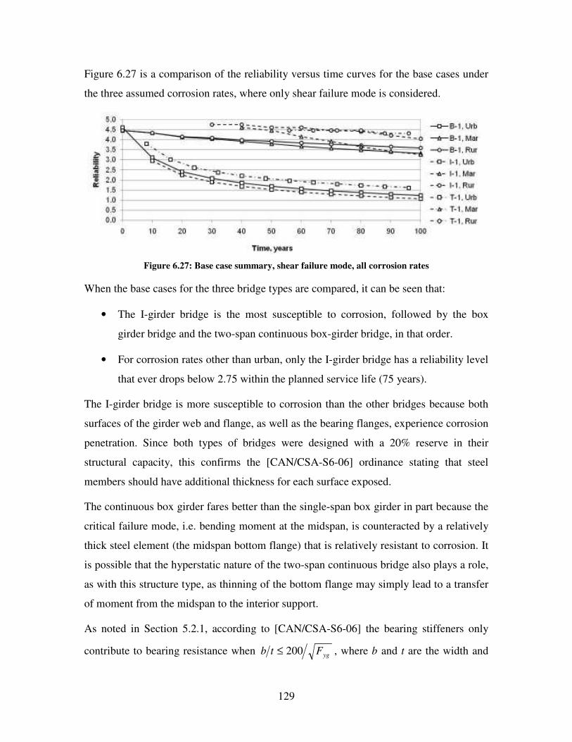
129

Figure 6.27 is a comparison of the reliability versus time curves for the base cases under

the three assumed corrosion rates, where only shear failure mode is considered.

Figure 6.27: Base case summary, shear failure mode, all corrosion rates

When the base cases for the three bridge types are compared, it can be seen that:

• The I-girder bridge is the most susceptible to corrosion, followed by the box

girder bridge and the two-span continuous box-girder bridge, in that order.

• For corrosion rates other than urban, only the I-girder bridge has a reliability level

that ever drops below 2.75 within the planned service life (75 years).

The I-girder bridge is more susceptible to corrosion than the other bridges because both

surfaces of the girder web and flange, as well as the bearing flanges, experience corrosion

penetration. Since both types of bridges were designed with a 20% reserve in their

structural capacity, this confirms the [CAN/CSA-S6-06] ordinance stating that steel

members should have additional thickness for each surface exposed.

The continuous box girder fares better than the single-span box girder in part because the

critical failure mode, i.e. bending moment at the midspan, is counteracted by a relatively

thick steel element (the midspan bottom flange) that is relatively resistant to corrosion. It

is possible that the hyperstatic nature of the two-span continuous bridge also plays a role,

as with this structure type, as thinning of the bottom flange may simply lead to a transfer

of moment from the midspan to the interior support.

As noted in Section 5.2.1, according to [CAN/CSA-S6-06] the bearing stiffeners only

contribute to bearing resistance when ygFtb 200≤ , where b and t are the width and

130

thickness of the stiffener and Fyg is the yield strength of the plate. According to [CISC

2006], the width-thickness limits are not related to the class of section, but are a function

of other considerations, i.e., the edge conditions and residual stresses of the component.

Because this slenderness ratio is a function of the yield stress of the girder, it introduces a

non-rational element into the bearing reliability calculations. For example, where the

yield strength is higher, a thicker plate is required for the bearing stiffener, even though

its maximum bearing stress (as opposed to overall resistance) is higher (see Equations 5.5

and 5.15). Where the use of higher strength steel should result in a smaller required

section, here the opposite is the result. Also, because steel strength is one of the statistical

variables, higher strength bearing plates result in immediate failure of the bridge, a result

which, again, is non-rational. Because of misconceptions which may result from this, the

bearing failure mode is not considered in the sensitivity studies.

6.3 Sensitivity Studies

6.3.1 Corrosion Scenario

Simply-Supported Box Girder Bridge

Figure 6.28 to Figure 6.30 show the shear and moment failure mode output for the B-1

box girder bridge subjected to the three corrosion rates and several different corrosion

“scenarios”. In these figures, the W+F corrosion scenario refers to corrosion of the web

and the flange together, while the F scenario refers to corrosion of the flange-only (see

Figure 5.10 for a diagram of the corrosion locations). Regarding the moment failure, the

first corrosion scenario can be thought of as a “worst case” scenario. The second was

considered herein as it was believed to be more representative of the corrosion observed

on overpass structures, in the splash zones of trucks passing underneath (see Figure 1.1).

131

Figure 6.28: Bridge B-1, urban corrosion rate, corrosion scenario varied

Figure 6.29: Bridge B-1, marine corrosion rate, corrosion scenario varied

Figure 6.30: Bridge B-1, rural corrosion rate, corrosion scenario varied

Based on Figure 6.28 to Figure 6.30, the following observations are made:

• At all corrosion rates, corrosion to the flange-only leads to a noticeable increase in

the reliability due to moment failure. However, there is a very significant increase

in the reliability relating to the shear resistance. The moment values are relatively

similar, but the shear values are very different.

132

• At the urban corrosion rate, the effect of web corrosion is noticeable; this is less

true for the marine corrosion rate, and not true for the rural corrosion rate.

• At the urban corrosion rate, the uncorroded web more than triples the service life

of the structure (15 years vs. 55 years).

I-Girder Bridge

Figure 6.31 to Figure 6.33 present the results of a similar set of analyses on the simply-

supported I-girder structure (Bridge I-1). In this case, however, three corrosion scenarios

are examined: corrosion to the web and both surfaces of the flange (W+F), corrosion to

both surfaces of the flange (F), and corrosion to the top of the flange-only (TOF) (see

Figure 5.5 for a diagram of the corrosion locations).

Shear failure, being consequent upon corrosion of the web, only occurred in the web +

flange corrosion scenario, so this is the only one to appear on the following figures.

Figure 6.31: Bridge I-1, urban corrosion rate, corrosion scenario varied

Figure 6.32: Bridge I-1, marine corrosion rate, corrosion scenario varied

133

Figure 6.33: Bridge I-1, rural corrosion rate, corrosion scenario varied

Based on Figure 6.31 to Figure 6.33, the following observations are made:

• At all corrosion rates, corrosion to the web and the flange together cause the

greatest decline in reliability; however, it is only at the urban corrosion rate that

this decline differs substantially from the other scenarios.

• At the urban corrosion rate, there is a significant difference in the results for the

different corrosion scenarios; however, at the lower corrosion rates the difference

diminishes to the point that it becomes negligible.

• At the marine and rural corrosion rates, the I-1 bridge does not drop below 3.25

over the 100 year analysis period.

The reason for the similarity between the reliability lines at the marine and rural

corrosion rates is that the web in fact contributes a relatively small amount to the moment

resistance.

Two-Span Continuous Box-Girder Bridge

Figure 6.34 to Figure 6.36 show the effect of progressive corrosion on the two-span

continuous box-girder bridge. In this case, both moment and shear failures occur.

134

Figure 6.34: Bridge T-1, urban corrosion rate, corrosion scenario varied

Figure 6.35: Bridge T-1, marine corrosion rate, corrosion scenario varied

Figure 6.36: Bridge T-1, rural corrosion rate, corrosion scenario varied

Based on the data in Figure 6.34 to Figure 6.36, the following observations are made:

• At the urban corrosion rate, the reliability curves for the moment failure mode

with and without corrosion to the web are very similar.

135

• At the urban corrosion rate, the effect of the shear failure modes is vastly

increased if the web is included in the corrosion scenario.

• At the marine and rural corrosion rates, the T-1 bridge does not drop below 3.25

over the 100 year analysis period, regardless of the corrosion scenario.

It should be noted that most of the moment failures for the two-span continuous bridge

are at the pier where negative bending occurs; the failures are a result of the flange failing

to provide sufficient compression resistance. This suggests again that the web does not

contribute significantly to the negative moment resistance.

Comparison

Based on the above results, the following observations are made:

• When only the flange is corroding, none of the bridge types has a shear reliability

value below 3.25 over a 100 year service life.

• Regarding moment resistance at the urban corrosion rate, the two-span bridge

appears to benefit least from flange-only corrosion, followed by the single-span

box girder and I-girder, respectively.

6.3.2 Highway Class

Box Girder Bridge

Figure 6.37 to Figure 6.39 show the reliability results for 40 m long box bridge, subject to

the various corrosion rates, and with different ADTT values (see Table 5.11 for these

values). The ADTT is related to the live load shear and moment bias factors.

Figure 6.37: Bridge B-1, urban corrosion rate, highway class varied

136

Figure 6.38: Bridge B-1, marine corrosion rate, highway class varied

Figure 6.39: Bridge B-1, rural corrosion rate, highway class varied

I-Girder Bridge

The results of a similar study are presented below for the 40 m long I-girder bridge.

Figure 6.40: Bridge I-1, urban corrosion rate, highway class varied

137

Figure 6.41: Bridge I-1, marine corrosion rate, highway class varied

Figure 6.42: Bridge I-1, rural corrosion rate, highway class varied

Comparison

Based on these figures, it can be concluded that the highway class is not an important

factor for either girder type. This can be explained by the fact that as the traffic volume

increases, the mean of the bias factor for the extreme live load effect tends to increase.

However, the standard deviation tends to decrease (see Table 5.11).

6.3.3 Girder Yield Strength

Box Girder Bridges

Figure 6.43 to Figure 6.45 show the results for bridges where the girders are composed of

steels with various yield strengths. The bridges being compared here are B-1 (Fyg = 350

MPa), B-2 (Fyg = 300 MPa), and B-3 (Fyg = 480 MPa). Note that the analysis in this

section assumes that all of the steel grades corrode at the same rate.

138

Figure 6.43: Bridges B-1, B-2, B-3, urban corrosion rate.

Figure 6.44: Bridges B-1, B-2, B-3, marine corrosion

Figure 6.45: Bridges B-1, B-2, B-3, rural corrosion

For the simply-supported box girder bridges with varying steel strengths:

• The reliability of the structures drops below 2.75 only in the case of urban

corrosion rate. At the marine and rural corrosion rates, the reliability does not

drop below 3.25 over the 100 year time frame.

139

• At the urban corrosion rate, the time-dependent reliability with respect to the

moment resistance of Bridge B-3 (Fyg = 480 MPa) drops faster than the other two

structures, but only by a small amount.

• Otherwise, there are no significant differences among the results for the three

bridges. The failure modes are tightly grouped for each corrosion rate.

Bridges B-1, B-2, and B-3 all have the same web thickness at the abutments and midspan

(12.7 mm and 11.1 mm respectively). As a result of this, the effect of steel yield strength

on the shear failure mode is not distinguishable. However, the flange thicknesses for B-1,

B-2, and B-3 are different (20.6 mm, 25.4 mm, and 12.7 mm respectively), and, at least at

the urban corrosion rate, the structure with the highest yield strength and thinnest bottom

flange also has the lowest reliability, if only by only a small margin.

I-Girder Bridges

Figure 6.46 to Figure 6.48 compare the reliability curves for the simply supported I-

girder bridges I-1 (Fyg = 350 MPa), I-2 (Fyg = 300 MPa), and I-3 (Fyg = 480 MPa).

Figure 6.46: Bridges I-1, I-2, I-3, urban corrosion rate.

140

Figure 6.47: Bridges I-1, I-2, I-3, marine corrosion rate

Figure 6.48: Bridges I-1, I-2, I-3, rural corrosion rate

For the I-girder bridges with various girder steel strengths:

• At the urban corrosion rate, the difference between the shear and moment failure

modes for the various bridges is negligible; however, at the other corrosion rates,

it is more significant, though at no point does the reliability drop below 2.75.

• At all three corrosion rates, the moment and shear bands are closely grouped.

• At the marine and rural corrosion rates, the lower reliability values of Bridge B-2

(Fyg =300 MPa) is a result of its lower reliability at year 0.

Regarding the moment failure, the results are counterintuitive: the bridge composed of

the lowest strength steel should be the most reliable, by virtue of its thicker section;

however, the results here suggest otherwise. The reason for this is that the high strength

steel has a higher initial reliability, and this advantage perdures through the test life;

however, at high corrosion rates the difference between the bridges is negligible.

141

Comparison

In general, these results favour high strength steel, since less steel is required and the self-

weight of the bridge is lower. While B-2 girder weighs approximately 3.5% more than

that of B-1, the B-3 girder weighs 19.8% less than that of B-1. The same is true for the I-

girder bridge: the I-2 girder weighs 5.9% more than the I-1 girder, while the I-3 girder

weighs 18.7% less than the I-1 girder. Thus there are potential savings to be made in the

reduced material used as the girder yield strength is increased, without causing a

significant reduction in the time-dependent reliability of the structure.

6.3.4 Bridge Span

Box Girder Bridges

Figure 6.49 to Figure 6.51 show the effect of girder span on the reliability of simply-

supported box girder bridges. The bridges being compared are B-1, B-4, and B-5, which

have 40 m, 30 m, and 35 m spans respectively.

Figure 6.49: Bridges B-1, B-4, B-5, urban corrosion

Figure 6.50: Bridges B1, B4, B5, marine corrosion rate.

142

Figure 6.51: Bridges B-1, B-4, B-5, rural corrosion rate.

For the simply-supported box girder bridges of varying lengths:

• At the urban corrosion rate, there is a noticeable difference between the shear

failure mode reliability curves of the different bridges, but the moment failure

reliability curves are very similar.

• There is also a substantial difference between the shear failure mode reliability

curves in the marine and rural corrosion rates.

• Bridge B-5 (35 m span) outperforms B-1 (40 m span) with respect to the shear

failure mode; this is due to the fact that they both have the same web thickness,

but B-1, being longer, has the larger shear values.

I-Girder Bridges

Figure 6.52 to Figure 6.54 relate to the simply-supported I-girder bridges of varying

lengths. I-1, I-4, and I-5 are 40 m, 30 m, and 35 m long, respectively.

143

Figure 6.52: Bridges I-1, I-4, I-5, urban corrosion rate.

Figure 6.53: Bridges I-1, I-4, I-5, marine corrosion rate.

Figure 6.54: Bridges I-1, I-4, I-5, rural corrosion rate.

For the simply-supported I-girder bridges with varying span lengths:

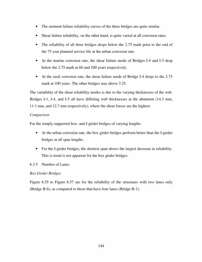
144

• The moment failure reliability curves of the three bridges are quite similar.

• Shear failure reliability, on the other hand, is quite varied at all corrosion rates.

• The reliability of all three bridges drops below the 2.75 mark prior to the end of

the 75 year planned service life at the urban corrosion rate.

• At the marine corrosion rate, the shear failure mode of Bridges I-4 and I-5 drop

below the 2.75 mark at 60 and 100 years respectively.

• At the rural corrosion rate, the shear failure mode of Bridge I-4 drops to the 2.75

mark at 100 years. The other bridges stay above 3.25.

The variability of the shear reliability modes is due to the varying thicknesses of the web.

Bridges I-1, I-4, and I-5 all have differing web thicknesses at the abutment (14.3 mm,

11.1 mm, and 12.7 mm respectively), where the shear forces are the highest.

Comparison

For the simply-supported box- and I-girder bridges of varying lengths:

• At the urban corrosion rate, the box girder bridges perform better than the I-girder

bridges at all span lengths.

• For the I-girder bridges, the shortest span shows the largest decrease in reliability.

This is trend is not apparent for the box girder bridges.

6.3.5 Number of Lanes

Box Girder Bridges

Figure 6.55 to Figure 6.57 are for the reliability of the structures with two lanes only

(Bridge B-6), as compared to those that have four lanes (Bridge B-1).

145

Figure 6.55: Bridges B-1 & B-6, urban corrosion rate

Figure 6.56: Bridges B-1 & B-6, marine corrosion rate

Figure 6.57: Bridges B-1 & B-6, rural corrosion rate

For the box girder bridges with two or four lanes:

• At all corrosion rates, the four-lane bridge is more susceptible to shear and

moment failure modes.

• At the marine and rural corrosion rates, the two-lane bridge does not fail in shear.

146

The reason for the relative susceptibility of the four-lane bridge may be that the web and

flange sections of the four-lane bridge are less thick than those of the two-lane bridge.

The additional thickness is required because of the weight of the sidewalks and barriers is

distributed to fewer girders, and the two-lane bridge has a higher modification factor for

live loading (0.9 to 0.7, see Table 5.5).

I-Girder Bridges

Figure 6.58 to Figure 6.60 show a similar comparison for the I-girder bridges.

Figure 6.58: Bridges I-1 & I-6, urban rate

Figure 6.59: Bridges I-1 & I-6, marine corrosion rate

147

Figure 6.60: Bridges I-1 & I-6, rural corrosion rate

For the I-girder bridges with two or four lanes:

• At all corrosion rates, the two-lane bridge (I-6) is more susceptible to the shear

failure mode than the four-lane bridge (I-1).

• At all corrosion rates, the four-lane bridge (I-1) is more susceptible to the moment

failure mode than the two-lane bridge (I-6)

Comparison

For the shear failure mode, the two-lane box girder bridge (I-6) is less susceptible than

the four-lane box girder bridge (I-1); however, this trend is reversed in the I-girder

bridges. The reason for this is that the initial reliability of the four-lane I-girder bridge (I-

6) with respect to shear failure is considerably higher than that of the two-lane bridge (I-

1). This initial structural advantage remains throughout the duration of the analysis.

6.3.6 Web Breathing Failure Mode

The base case bridges (B-1 & I-1) were also analysed for their resistance to the web

breathing limit state (see Section 5.2.1).

Box Girder Bridge

Figure 6.61 shows the results of these tests, for all three corrosion rates, where the

comparison is made between the total failure due to the combined ultimate limit states

(U) versus the web breathing limit state (WB) on its own.

148

Figure 6.61: Bridge B-1, ULS vs. WB, all corrosion rates

For the box girder bridge:

• The web breathing limit state is never more critical than the ultimate limit states

for the box girder bridge.

• The fatigue limit state is likely to affect structural performance only at the urban

corrosion rate.

I-Girder Bridge

Figure 6.62 shows a similar comparison for an I-girder bridge.

Figure 6.62: Bridge I-1, ULS vs. WB, all corrosion rates

For the I-girder bridge:

• The ULS cases cause a more significant decline in reliability than web breathing.

• Only at the urban corrosion rate is there an unacceptable risk of a web breathing

“failure” occurring during the lifespan of the structure.

149

Comparison

Figure 6.63 compares the web breathing behaviour of the box and I-girder bridges.

Figure 6.63: Bridges B-1 and I-1, web breathing comparison, all corrosion rates

For the girder type comparison of the web breathing limit state:

• The web breathing behaviour of the I-girder bridge is in all cases slightly worse

than that of the box girder bridge.

While the webs are 1/16” thicker on the I-girder bridge (I-1) than the box girder bridge

(B-1), they are also attacked from both sides by corrosion, and this makes them more

susceptible over time to web breathing failure mode.

6.3.7 Sensitivity Study Summary

General

Two trends in the sensitivity studies are worth noting. First, the idea of a statistical

“noise” should be understood. In the probability program, 14 different parameters are

varied statistically. Some of these parameters have a more significant impact than others.

For example, the corrosion rate has a significant impact, while the highway class does

not. The reason that no difference is visible in the highway class variation data (see

Figure 6.37 to Figure 6.42) is that, with the numerous parameters being varied

simultaneously, a change of one value may be overridden.

The other trend worth noting is the effect of using plate that comes in 1/16” (1.6 mm)

increments. This led to a certain “coarseness” in the design of some bridges, which in

turn is visible in the reliability data that the analyses produce. One such example of this is

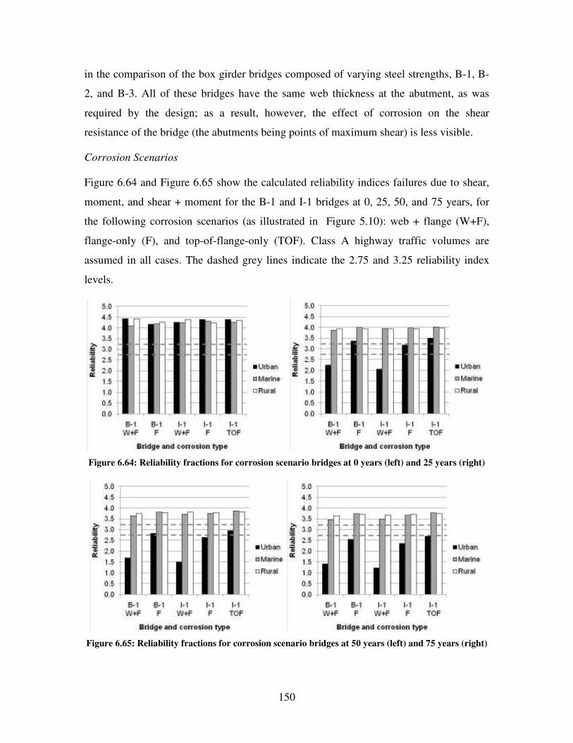
150

in the comparison of the box girder bridges composed of varying steel strengths, B-1, B-

2, and B-3. All of these bridges have the same web thickness at the abutment, as was

required by the design; as a result, however, the effect of corrosion on the shear

resistance of the bridge (the abutments being points of maximum shear) is less visible.

Corrosion Scenarios

Figure 6.64 and Figure 6.65 show the calculated reliability indices failures due to shear,

moment, and shear + moment for the B-1 and I-1 bridges at 0, 25, 50, and 75 years, for

the following corrosion scenarios (as illustrated in Figure 5.10): web + flange (W+F),

flange-only (F), and top-of-flange-only (TOF). Class A highway traffic volumes are

assumed in all cases. The dashed grey lines indicate the 2.75 and 3.25 reliability index

levels.

Figure 6.64: Reliability fractions for corrosion scenario bridges at 0 years (left) and 25 years (right)

Figure 6.65: Reliability fractions for corrosion scenario bridges at 50 years (left) and 75 years (right)

151

Figure 6.64 and Figure 6.65 show that the greatest degradation of the reliability level

occurs at the I-girder bridge that experiences corrosion to its web and both sides of its

bottom flange. However, this is closely followed by the web + flange corrosion to the box

girder; this is interesting because the I-girder is being attacked from both sides of its web

and bottom flange, while the box girder is attacked on one side only. This result is

mirrored by the flange-only corrosion to the B-1 and I-1 bridges. Not surprisingly, the I-1

bridge with corrosion occurring to its top flange-only fares the best.

Bridge Types

Figure 6.66 to Figure 6.69 are bar charts of the reliability indices for the twelve bridge

types at 25, 50, and 75 year spans, respectively. They correspond with combined failure

due to shear, moment, and shear + moment. All the bridges being considered here are

assumed to experience web + flange corrosion and Class A highway traffic volumes.

Again, the dashed grey lines are at the 2.75 and 3.25 levels.

Figure 6.66: Reliability fraction of bridge types at 0 years

152

Figure 6.67: Reliability fraction of bridge types at 25 years

Figure 6.68: Reliability fraction of bridge types at 50 years

Figure 6.69: Reliability fraction for bridge types at 75 years

Of all the bridges, the one that fares the worst from corrosion is the 30 m long I-girder

bridge (I-4), with the 35 m I-girder bridge (I-5) coming next. These bridges have a low

153

reliability because their shorter length enabled the use of thinner plate for their webs;

since corrosion progresses at the same rate regardless of the thickness of the steel, these

bridges experienced the fastest degradation.

Except for the I-4 and I-5 bridges, all the bridges maintain a reliability level above 3.25

up to the 75 year mark at the marine and rural corrosion rates. Thus, it can be assumed

that if a bridge only shows a normal patina and does not give evidence of significant

corrosion, it will perform adequately for the duration of its service life.

6.4 Case Study

Design and maintenance data has been made available for two box girder bridges along

Highway 402, between London, Ontario and Sarnia, Ontario. Both bridges are four-lane,

four-girder highway overpasses. Both are 83.0 m long, divided into two equal, simply-

supported composite box girder spans. However, girder plate thicknesses, slab widths,

sidewalk dimensions, etc, are different. Their truck traffic is estimated to be that of Class

C structures. Figure 6.70 and Figure 6.71 show the resistance fractions of the two bridges,

henceforth labelled A and B.

Figure 6.70: Bridge A resistance fractions

154

Figure 6.71: Bridge B resistance fractions

Figure 6.72 and Figure 6.73 are the reliability output for both bridges at the urban

corrosion rate, with the bridge geometry taken from their respective structural drawings.

For all analyses of these bridges, it was assumed that corrosion to the web and flange

occur for 3.0 m from each abutment, and corrosion to the flange-only occurs over

approximately 15.0 m centred at the midspan section. This is in accordance with what

was noted during site visits to both bridges.

Figure 6.72: Bridge A, urban corrosion rate

155

Figure 6.73: Bridge B, urban corrosion rate

An inspection performed 26 years after their construction; as part of this inspection,

readings were taken of the material thicknesses at the web and flange of the girders.

Inspections were performed at midspan and both abutments for every girder. A series of

five readings were taken from side to side of each member. Figure 6.74 shows the points

where thickness measurements were taken at all abutment and midspan locations.

&*!

&*+

&*,

&*-

&*.

&*/

&*0

&*1

&*2

&!*

&!!

&!+

&!,

&!-

&!.

&!/

&!0

&!1

&!2

&+*

Figure 6.74: Inspection thickness measurement locations

This data can be used to recalculate the reliability, as is shown in the following figures. In

Figure 6.75 and Figure 6.76, the time-dependent reliability of the bridges was

recalculated using the average measured plate thicknesses for the web and flange at the

abutments and midspan, but keeping the urban corrosion rate (which was in keeping with

the high level of corrosion on the structures). The plate thicknesses recorded were almost

all larger than expected, and even larger than designed; this is the reason for the increase

in reliability in these figures.

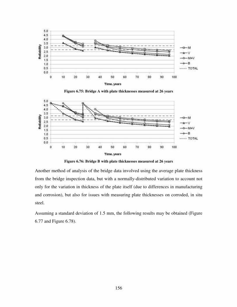
156

Figure 6.75: Bridge A with plate thicknesses measured at 26 years

Figure 6.76: Bridge B with plate thicknesses measured at 26 years

Another method of analysis of the bridge data involved using the average plate thickness

from the bridge inspection data, but with a normally-distributed variation to account not

only for the variation in thickness of the plate itself (due to differences in manufacturing

and corrosion), but also for issues with measuring plate thicknesses on corroded, in situ

steel.

Assuming a standard deviation of 1.5 mm, the following results may be obtained (Figure

6.77 and Figure 6.78).

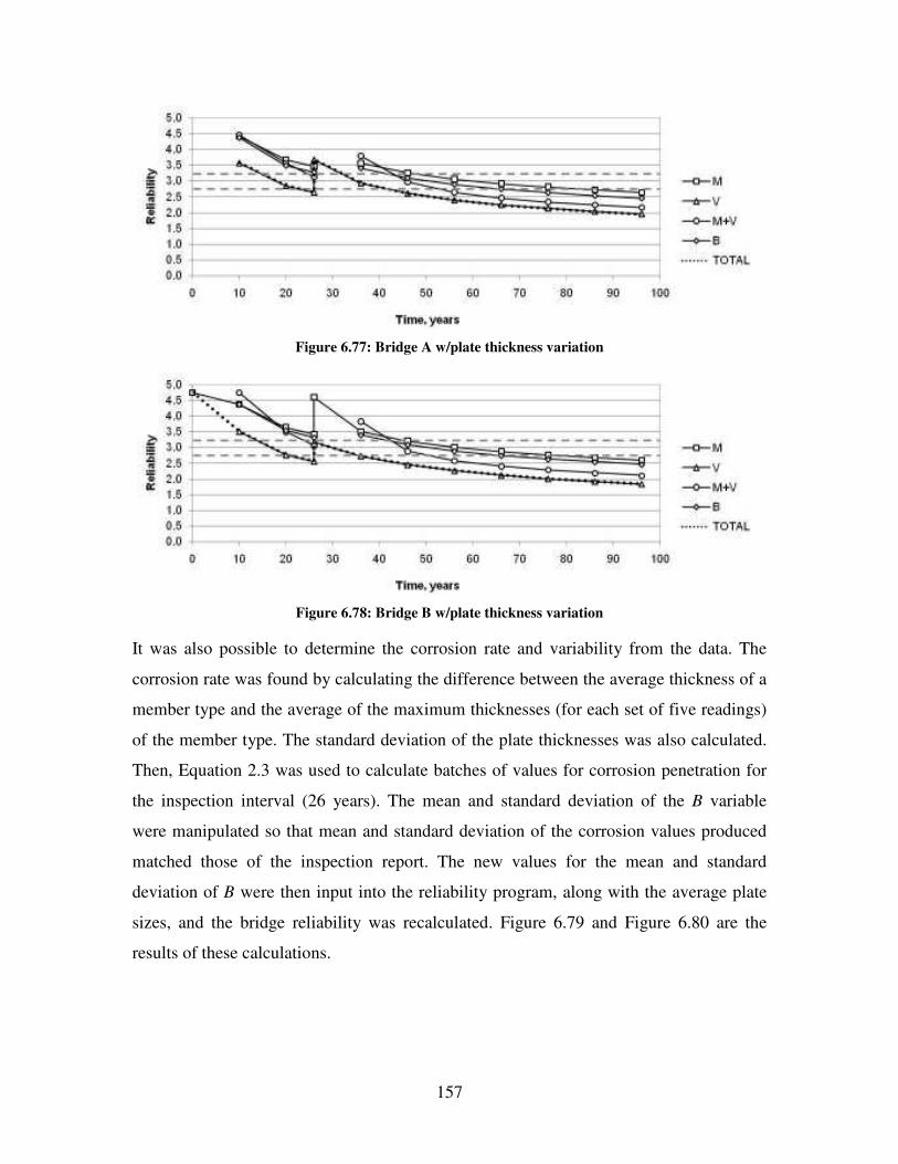
157

Figure 6.77: Bridge A w/plate thickness variation

Figure 6.78: Bridge B w/plate thickness variation

It was also possible to determine the corrosion rate and variability from the data. The

corrosion rate was found by calculating the difference between the average thickness of a

member type and the average of the maximum thicknesses (for each set of five readings)

of the member type. The standard deviation of the plate thicknesses was also calculated.

Then, Equation 2.3 was used to calculate batches of values for corrosion penetration for

the inspection interval (26 years). The mean and standard deviation of the B variable

were manipulated so that mean and standard deviation of the corrosion values produced

matched those of the inspection report. The new values for the mean and standard

deviation of B were then input into the reliability program, along with the average plate

sizes, and the bridge reliability was recalculated. Figure 6.79 and Figure 6.80 are the

results of these calculations.

158

Figure 6.79: Bridge A with measured plate thicknesses and corrosion rates

Figure 6.80: Bridge B with measured plate thicknesses and corrosion rates

Figure 6.81 and Figure 6.82 show a summary of the total failures due to ULS for both

bridges. For these figures, Method 1 refers to the unmodified reliability analysis, Method

2 refers to the analysis with the updated plate thicknesses only, Method 3 refers to the

updated plate thicknesses plus the statistical variation of the thicknesses, and Method 4

refers to the updated plate thicknesses plus the substitution of recalculated corrosion rates

and variances.

159

Figure 6.81: Bridge A, summary of reliability calculation modes

Figure 6.82: Bridge B, summary of reliability calculation modes

Table 6.10 shows the percentage benefit gained by collecting and analysing data from the

plate girder bridges. The data below compares the original amount of time it took the

bridge to reach a reliability of 2.75, against the recalculated amount of time to reach this

level.

Table 6.10: Recalculated bridge service lives

Bridge A Bridge B

Method 2 91% 95%

Method 3 82% 66%

Method 4 No failure 166%

160

CHAPTER 7: CONCLUSIONS AND RECOMMENDATIONS

7.1 Conclusions

The conclusions presented in this chapter are divided into the three main areas of the

research work: those resulting from (i) the ultrasonic thickness gauge (UTG) studies, (ii)

the protective coating corrosion testing studies, and (iii) the development of the

structural analysis models and the analytical studies performed with these models.

7.1.1 UTG Thickness Measurement Studies

Regarding the use of the UTG for the inspection of steel plate experiencing section loss

due to corrosion, the following conclusions are drawn:

• The instrument is not capable of measuring from a heavily pitted surface, even if

the rust layer has been removed (e.g. by sandblasting or chemical wash), because

the surface is too uneven to provide a sufficiently uniform contact between the

steel and the UTG probe head.

• When the measurements are made of a weathering steel plate with corrosion

product on the opposite side, the UTG does not include the thickness of corrosion

product in the measured plate thickness and, therefore, will provide values

suitable for service life prediction.

• When measurements are made of a weathering steel plate with corrosion product

on the same side then, if a measurement is possible at all, the measured thickness

includes the corrosion layer, and this layer appears thicker than it actually is.

Therefore the data cannot be used in service life predictions without further

analysis to correct for the effect of the corrosion product.

• The UTG measures the shortest distance to an opposing surface; as such, it can be

expected to measure the distance to a pit on the opposite side of the plate. In order

to accurately determine the lowest plate thickness measurement, however, the

UTG probe head must be directly over the pit.

161

7.1.2 Protective Coating Corrosion Testing Studies

The following conclusions are drawn from the corrosion test studies presented herein of

uncoated, metallized, and zinc-tape coated weathering steel specimens, and the

subsequent analyses of the corroded specimens:

• All the protective coatings tested, including pure zinc and aluminum-zinc-indium

alloy metallizing and PVC-coated zinc tape, were successful in preventing

corrosion of the weathering steel specimens in the period of the accelerated test

which was estimated to be equivalent to 40 years of natural exposure.

• The surface roughness of the specimen did not have any detectable influence on

the effectiveness of the metallizing or zinc tape protective coating.

• The effectiveness of the metallizing and zinc tape protective coatings was not

reduced by the degree of sandblasting performed on the structure. More

specifically, the results indicate that sandblasting the structure to a sub-white

metal condition was not necessary for effective performance of these coatings.

• The metallizing and tape coatings had equal success at protecting the steel from

structures constructed 40 years ago and the steel available for structures today.

7.1.3 Modelling of Corroding Weathering Steel Highway Structures

The following conclusions are drawn as a result of the development of the structural

models for assessing the remaining service lives of corroding weathering steel highway

structures and the analytical studies performed using these models:

• Corrosion occurring at the urban rate to weathering steel structures is capable of

significantly reducing their service life. The reliability of the standard box girder

bridge analysed herein drops below the acceptable level of 2.75 in approximately

15 years, rather than the 75 years required by [CAN/CSA-S6-06]. Likewise, the

reliability of the I-girder bridge is below 2.75 after 13 years, and the two-span box

girder bridge is below 2.75 after 22 years. Marine and rural corrosion rates do not

pose a challenge to highway structures, except in the case of short-span, simply

supported (� 35 m) I-girder bridges. These bridges are threatened because, unlike

the box girder bridges, their girder webs are both thinner than those of the longer

162

spans, and attacked from both sides by corrosion. In all other cases, the bridge

reliability does not drop below 2.75 over a 75 year service life.

• The two-span box girder bridge has a reliability of 1.77 after 75 years at the urban

corrosion rate, as compared with the simply-supported box girder and I-girder

bridges which have reliabilities of 1.42 and 1.24 at this point,.

• The bearing failure mode is problematic for time-dependent reliability calculation

according to the equations provided in [CAN/CSA-S6-06] because of the

slenderness equation, which displays a non-rational bias against high-strength

steel.

• Web + flange corrosion causes a more rapid degradation to the box and I-girder

bridges than flange-only corrosion. For the web + flange corrosion scenario, shear

is the predominant failure mode, while for the flange-only corrosion scenario it is

moment. For the box girder bridge at the urban corrosion rate, corrosion to the

flange-only results in a reliability of 2.55 after 75 years, compared with 1.42 if

both the web and the flange are subject to corrosion; this difference is

substantially less at the other corrosion rates. For the I-girder bridge at the urban

corrosion rate, the reliability at 75 years is 2.37 for the scenario where both sides

of the flange corrode and 2.70 where only the top of the flange corrodes,

compared with 1.24 where web + flange corrosion is occurring. For the two-span

box girder bridge at the urban corrosion rate, corrosion to the flange-only results

in a reliability of 2.07 after 75 years; corrosion to the web and flange together

results is a reliability of 1.76.

• The difference between the effects of web + flange corrosion for the box and I-

girder bridges is relatively minor. The same is true for flange-only corrosion for

these bridges. Nevertheless, the I-girder bridges are more sensitive to corrosion

than box-girder bridges at both types of corrosion.

• Over the long term, shear failure mode is critical because of the relative

slenderness of the plate. The amount of time required for this to occur depends on

the corrosion rate.

163

• The use of high strength steel for the bridge girder does not have a significant

impact on the service life of the highway structure. While it was expected that

higher strength steel would result in thinner sections that are more susceptible to

corrosion, this is not seen in the analysis results. After 75 years at the urban

corrosion rate, a box girder bridge with 480 MPa yield strength has a reliability of

1.48, as opposed to 1.42 for a girder with 350 MPa yield strength. For the I-girder

bridge, the 480 MPa bridge’s reliability is 1.23, as opposed to 1.24 for the 350

MPa bridge. The use of low strength steel likewise does not have a significant

impact. After 75 years at the urban corrosion rate, a 300 MPa yield strength box

girder bridge has a reliability of 1.50, compared with 1.42 for the 350 MPa box

girder structure. For the I-girder structure, the 300 MPa bridge has a reliability of

1.25 after 75 years, while the 350 MPa bridge has a reliability of 1.24.

• For the box girder structures, shorter spans do not result in a significantly

different reliability after 75 years at the urban corrosion rate. The 30, 35, and 40

m long box girder bridges have reliabilities of 1.47, 1.65, and 1.42, respectively.

The difference in these values is more a result of the initial reliability of the

bridges. For the 30, 35, and 40 m long I-girder bridges, the reliability values are

0.84, 1.08, and 1.24, respectively. This shows the effect of thinner webs which

undergo corrosion on both exposed faces.

• The number of lanes appears to have an impact on the time-dependent reliability

of the structure, insofar as a structure with fewer lanes will have larger girders,

which will in turn be more resistant to corrosion penetration. The box girder

bridge at the urban corrosion rate has a reliability of 1.74 at the 75 year mark,

while the four-lane bridge has a reliability of 1.42. However, for the I-girder

bridge, this effect is not visible due to the relatively low initial reliability of the

two-lane bridge design.

• The traffic amount does not have a significant impact on the time-dependent

reliability of a bridge. At 75 years, the bridge supporting a Class A highway

performs marginally worse than those supporting Class B, C, and D highways (at

the urban corrosion rate, 1.42 to 1.51, 1.52, and 1.52, respectively). For the I-

164

girder bridge, after 75 years at the urban corrosion rate the Class A highway

bridge reliability is 1.24, while the Class B, C, and D highway structures are 1.25,

1.27, and 1.29.

• The fatigue limit state of web breathing does not have a more decisive impact

than the ultimate limit states. After 75 years at the urban corrosion rate, the

reliability is 1.47 for this fatigue limit state for the box girder, and 1.33 for the I-

girder bridge, as compared to 1.42 and 1.24 for the structures at the shear,

moment, and shear + moment limit states.

• Very significant gains to the predicted service life (ranging from a 66% increase

to no predicted failure whatsoever) can be made by integrating data from a

particular bridge into a reliability analysis.

7.2 Recommendations for Future Work

7.2.1 Protective Coating Corrosion Testing Studies

The following recommendations are made based on the corrosion testing studies

presented herein of uncoated, metallized, and zinc-tape coated weathering steel

specimens, and the subsequent analysis of the corroded specimens:

• Additional test parameters, such as the effect of sulphur oxides and scoring on the

metallized specimen performance, should be explored.

• The effect of a seam in the zinc tape, especially where the where the surface being

covered is uneven, should be studied by further corrosion testing.

• A life-cycle cost comparison of painting versus metallizing or zinc taping would

be beneficial. This comparison should take into account the maintenance costs of

each coating method as well as the environmental impacts/costs.

• Field trials of the metallizing and zinc tape coatings are recommended.

7.2.2 Modelling of Corroding Weathering Steel Highway Structures

The following recommendations are made as a result of the development of the structural

models for assessing the remaining service lives of corroding weathering steel highway

structures and the analytical studies performed using these models:

165

• Further research on the effects of corrosion on bridge deflection and other service

limit states, as well as the fatigue limit state, is recommended.

• More data are required about the corrosion rates of weathering steel. A good place

to get this data would be from a detailed survey of weathering steel bridges, for

example.

• Additional research should be done into two-span bridges, which appear to offer a

considerable benefit over the simply-supported bridges with respect to time-

dependent reliability.

166

REFERENCES

Albrecht, P. & Naeemi, A.H. National Cooperative Highway Research Program Report

272: Performance of Weathering Steel in Bridges. Transportation Research Board,

National Research Council, Washington, D.C., 1984.

Albrecht, P. & Hall, T.T. Atmospheric Corrosion Resistance of Structural Steels. Journal

of Materials in Civil Engineering, Vol. 15, No. 1, pp. 2-24, February 1, 2003.

Albrecht, P., Coburn, S.K., Wattar, F. M., Tinklenberg, G., & Gallagher, W. P. ().

National Cooperative Highway Research Program Report 314: Guidelines for the Use of

Weathering Steel in Bridges. Transportation Research Board, National Research Council,

Washington, D.C., 1989.

Ang, A. & Tang, W. Probability Concepts in Engineering Planning and Design. John

Wiley & Sons. New York. 1984.

Antaki, G. Fitness-for-Service and Integrity of Piping, Vessels, and Tanks. McGraw-Hill,

New York. 2005.

ASTM International. ASTM A 242/A 242M-04: Standard Specification for High-Strength

Low-Alloy Structural Steel. Annual Book of ASTM Standards 2007, Vol. 01.04. ASTM

International. 2007.

ASTM International. ASTM A 588/A 588M-05: Standard Specification for High-Strength

Low-Alloy Structural Steel, up to 50 ksi [345 MPa] Minimum Yield Point, with

Atmospheric Corrosion Resistance. Annual Book of ASTM Standards 2007, Vol. 01.04.

ASTM International. 2007.

ASTM International. ASTM A 709/A 709M-06a: Specification for Structural Steel for

Bridges. Annual Book of ASTM Standards 2007, Vol. 01.04. ASTM International. 2007.

ASTM International. ASTM D 1976-02: Standard Test Method for Elements in Water by

Inductively-Coupled Argon Plasma Atomic Emission Spectroscopy. Annual Book of

ASTM Standards 2007, Vol.11.01. ASTM International. 2007.

ASTM International. ASTM E 1019-03: Standard Test Methods for Determination of

Carbon, Sulfur, Nitrogen, and Oxygen in Steel, Iron, Nickel, and Cobalt Alloys by

167

Various Combustion and Fusion Techniques. Annual Book of ASTM Standards 2007,

Vol. 03.05. ASTM International. 2007.

ASTM International. ASTM G 1-03: Standard Practice for Preparing, Cleaning, and

Evaluating Corrosion Test Specimens. Annual Book of ASTM Standards 2007, Vol.

03.02. ASTM International. 2007.

ASTM International. ASTM G 101-04: Standard Guide for Estimating the Atmospheric

Corrosion Resistance of Low-Alloy Steels. Annual Book of ASTM Standards 2007, Vol.

03.02. ASTM International. 2007.

Cheung, M.S. & Li, W.C. Reliability assessment in highway bridge design. Canadian

Journal of Civil Engineering Vol. 29, pp. 799–805, 2002.

Cheung, M.S. & Li, W.C. Serviceability reliability of corroded steel bridges. Canadian

Journal of Civil Engineering Vol. 28, pp. 419–424, 2001.

CISC. Handbook of Steel Construction, 9th Edition. Canadian Institute of Steel

Construction. 2006.

Cook, D.C. Spectroscopic Identification of Protective and Non-Protective Corrosion

Coatings on Steel Structures in Marine Environments. Corrosion Science Vol. 47, pp.

2550–2570, 2005.

CSA. CAN/CSA-G40.20-04: General requirements for rolled or welded structural quality

steel. Canadian Standards Association. February 2004.

CSA. CAN/CSA-G40.21-04: Structural quality steel. Canadian Standards Association.

February 2004.

CSA. Calibration Report for CAN/CSA-S6-06 Canadian Highway Bridge Design Code.

Pdf. 2007.

CSA. CAN/CSA-S6-06: Canadian Highway Bridge Design Code. A National Standard of

Canada. Canadian Standards Association. Pdf.

CSA. CAN/CSA-S6.1-00: Commentary on CAN/CSA-S6-00, Canadian Highway Bridge

Design Code. Pdf.

168

Czarnecki, A.A. System Reliability Models for the Evaluation of Corroded Steel Girder

Bridges. Thesis. University of Michigan, 2006.

Czarnecki, A.A. & Nowak, A.S. Time-Variant Reliability Profiles for Steel Girder

Bridges. Structural Safety Vol. 30 No. 1, pp. 49-64, 2006.

Eamon, C.D., Nowak, A.S. Effect of Secondary Elements on Bridge Structural System

Reliability Considering Moment Capacity. Structural Safety Vol. 26, pp. 29–47, 2004.

Hara, S., Kamimura, T., Miyuki, H., & Yamashita, M. Taxonomy for Protective Ability of

Rust Layer Using Its Composition Formed on Weathering Steel Bridge. Corrosion

Science Vol. 49, pp. 1131–1142, 2007.

Jones, Denny. Principles and Prevention of Corrosion. 2nd Ed. Prentice Hall, New Jersey,

1996.

Kamimura, T., Hara, S., Miyuki, H., Yamashita, M., Uchida, H., Composition and

Protective Ability of Rust Layer Formed on Weathering Steel Exposed to Various

Environments, Corrosion Science Vol. 48, pp. 2799–2812, 2006.

Kayser, J.R. The Effects of Corrosion on Steel Girder Bridges. Thesis. University of

Michigan, 1988.

Kayser, J.R. & Nowak, A.S. Reliability of Corroded Steel Girder Bridges. Structural

Safety, Vol. 6, pp. 53–63 , 1989.

Kennedy, D.J.L., & Baker, K.A. Resistance Factors for Steel Highway Bridges. Canadian

Journal of Civil Engineering, Vol. 11, pp. 324–334, 1984.

Kulak, G.L. & Grondin, G.Y. Limit States Design in Structural Steel, Eighth Edition.

Canadian Institute of Steel Construction Inc., 2006.

Kulicki, J.M., Prucz, Z., Sorgenfrei, D.F., & Mertz, D.R. National Cooperative Highway

Research Program Report 333: Guidelines for Evaluating Corrosion Effects in Existing

Steel Bridges. Transportation Research Board, National Research Council, Washington,

D.C., 1990.

169

Kuroda, S., Kawakita, J., & Takemoto, M. An 18-Year Exposure Test of Thermal-

Sprayed Zn, Al, and Zn-Al Coatings in Marine Environment. Corrosion, Vol. 62, No. 7,

November 2005.

Laumet, P. Reliability-Based Deterioration Model for Deflection Limit State in Steel

Girder Bridges. Thesis. University of Michigan. 2006.

Legault, R.A. & Leckie, H.P., “Effect of Alloy Composition on the Atmospheric

Corrosion Behavior of Steels Based on a Statistical Analysis of the Larrabee-Coburn

Data Set,” Corrosion in Natural Environments: ASTM STP 558, American Society for

Testing and Materials, pp. 334-347, 1974.

Matthes, S.A., Cramer, S.D., Bullard, S.J., Covino, Jr., B.S. & Holcomb, G.R.

Atmospheric Corrosion and Precipitation Runoff from Zinc and Zinc Alloy Surfaces.

Presented as Paper No. 03598 at Corrosion 2003, 2003.

McCuen, R.H., & Albrecht, P.M. “Composite Modeling of Atmospheric Corrosion

Penetration Data,” Application of Accelerated Corrosion Tests to Service Life Prediciton

of Materials: ASTM 1194, Cragnolino, G. & Sridhar, N., Eds. American Society for

Testing and Materials, Philadelphia, pp. 65-102, 1994.

McCuen, R.H. & Albrecht, P.M. Effect of Alloy Composition on Atmospheric Corrosion

of Weathering Steel. Journal of Materials in Civil Engineering, Vol. 17, No. 2, pp. 117–

125, 2005.

McCuen, R.H. & Albrecht, P.M. Reanalysis of Thickness Loss Data for Weathering Steel.

Journal of Materials in Civil Engineering, Vol. 16, No. 3, pp. 237-246, 2004.

Melchers, R. Structural Reliability Analysis and Prediction, 2nd Edition. John Wiley &

Sons. 2002.

Misawa, T., Asami, K., Hashimoto, K. & Shimodaira, S. The Mechanism of Atmospheric

Rusting and the Protective Amorphous Rust on Low Alloy Steel. Corrosion Science, Vol.

14, pp. 279-289, 1974.

Park C.H. Time Dependent Reliability Models for Steel Girder Bridges. Thesis.

University of Michigan, 1999.

170

Sagüés, A.A. & Powers, R.G. Sprayed-Zinc Sacrificial Anodes for Reinforced Concrete

in Marine Service. Presented as paper no. 515 at Corrosion/95, 1995.

Sarveswaran J., Smith J.W. & Blockley, D.I. Reliability of Corrosion-Damaged Steel

Structures Using Internal Probability Theory. Structural Safety Vol. 20, pp. 237-255,

1998.

Society of Automotive Engineers. SAE J2334: Cosmetic Corrosion Lab Test – October

2002. SAE Handbook. 2003.

Society for Protective Coatings. Joint Surface Preparation Standard SSPC-SP 5/NACE

No. 1: White Metal Blast Cleaning. Pdf. 2000.

Tabsh, S. & Nowak, A. Reliability of Highway Girder Bridges. ASCE Journal of

Structural Engineering, Vol. 117 (8), pp. 2372–2388, 1991.

Townsend, H.E. & Zoccola, J.C. “Eight-Year Atmospheric Corrosion Performance of

Weathering Steel in Industrial, Rural, and Marine Environments,” Atmospheric

Corrosion of Metals: ASTM STP 767, S.W. Dean, Jr., & E.C. Rhea, Eds., American

Society for Testing and Materials, 1982, pp. 45-59.

Walbridge, S. A Probabilistic Study of Fatigue in Post-Weld Treated Tubular Bridge

Structures. EPFL Thesis No. 3330. École Polytechnique Fédérale de Lausanne, 2005.

Wang, J.H., Wei, F.I., Chang, Y.S. & Shih, H.C. The Corrosion Mechanisms of Carbon

Steel and Weathering Steel in SO2 Polluted Atmospheres. Materials Chemistry and

Physics Vol. 47, pp. l-8, 1997.

171

APPENDICES

172

APPENDIX A: CANADIAN WEATHERING STEEL SPECIFICATIONS

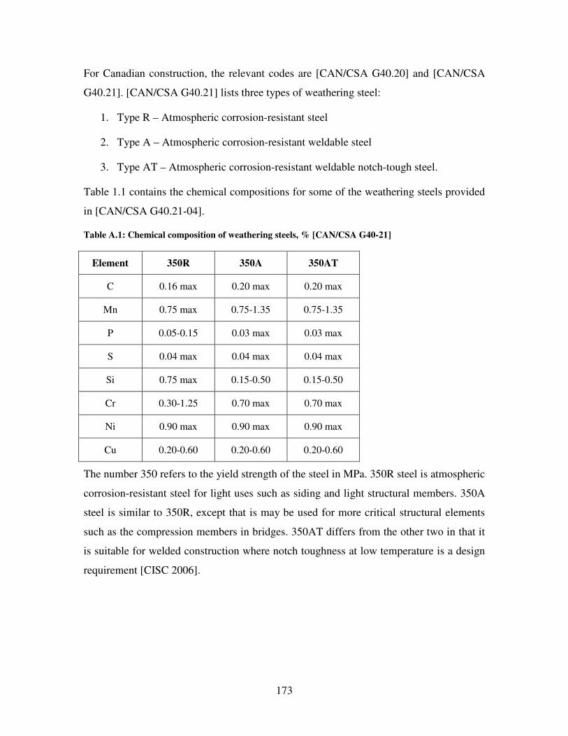
173

For Canadian construction, the relevant codes are [CAN/CSA G40.20] and [CAN/CSA

G40.21]. [CAN/CSA G40.21] lists three types of weathering steel:

1. Type R – Atmospheric corrosion-resistant steel

2. Type A – Atmospheric corrosion-resistant weldable steel

3. Type AT – Atmospheric corrosion-resistant weldable notch-tough steel.

Table 1.1 contains the chemical compositions for some of the weathering steels provided

in [CAN/CSA G40.21-04].

Table A.1: Chemical composition of weathering steels, % [CAN/CSA G40-21]

Element 350R 350A 350AT

C 0.16 max 0.20 max 0.20 max

Mn 0.75 max 0.75-1.35 0.75-1.35

P 0.05-0.15 0.03 max 0.03 max

S 0.04 max 0.04 max 0.04 max

Si 0.75 max 0.15-0.50 0.15-0.50

Cr 0.30-1.25 0.70 max 0.70 max

Ni 0.90 max 0.90 max 0.90 max

Cu 0.20-0.60 0.20-0.60 0.20-0.60

The number 350 refers to the yield strength of the steel in MPa. 350R steel is atmospheric

corrosion-resistant steel for light uses such as siding and light structural members. 350A

steel is similar to 350R, except that is may be used for more critical structural elements

such as the compression members in bridges. 350AT differs from the other two in that it

is suitable for welded construction where notch toughness at low temperature is a design

requirement [CISC 2006].

174

APPENDIX B: INDIVIDUAL SPECIMEN MASS LOSS DATA

175

Figure B.1: Uncoated old steel specimens

Figure B.2: Uncoated new steel specimens

Figure B.3: Aluminum alloy metallized, fully-sandblasted, new steel specimens

176

Figure B.4: Zinc metallized, fully-sandblasted, old steel specimens

Figure B.5: Zinc metallized, fully-sandblasted, new steel specimens

Figure B.6: Zinc metallized, partially-sandblasted, old steel specimens

177

Figure B.7: Zinc metallized, partially-sandblasted, new steel specimens

Figure B.8: Zinc taped, fully-sandblasted, old steel specimens

Figure B.9: Zinc taped, fully-sandblasted, new steel specimens

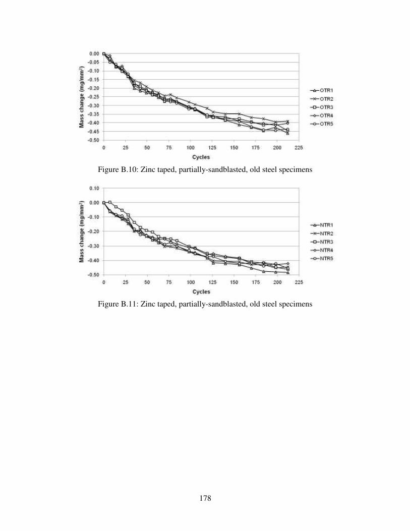
178

Figure B.10: Zinc taped, partially-sandblasted, old steel specimens

Figure B.11: Zinc taped, partially-sandblasted, old steel specimens