Vol.:(0123456789)1 3

Climate Dynamics https://doi.org/10.1007/s00382-018-4492-9

Prediction and predictability of tropical intraseasonal convection: seasonal dependence and the Maritime Continent prediction barrier

Shuguang Wang1  · Adam H. Sobel1,2 · Michael K. Tippett1 · Fréderic Vitart3

Received: 14 June 2018 / Accepted: 8 October 2018 © Springer-Verlag GmbH Germany, part of Springer Nature 2018

AbstractPrediction and predictability of tropical intraseasonal convection in the WMO subseasonal to seasonal (S2S) forecast data-base is assessed using the real-time OLR based MJO (ROMI) index. ROMI prediction skill in the S2S models, as measured by the maximum lead time at which the bivariate correlation coefficient between forecasts and observations exceeds 0.6, ranges from ~ 15 to ~ 36 days in boreal winter, which is 5–10 days higher than the MJO circulation prediction skill based on the MJO RMM index. ROMI prediction skill is systematically lower by 5–10 days in summer than in winter. Predictability measures show similar seasonal contrast in the two seasons. These results indicate that intraseasonal convection is inherently less predictable in summer than in winter. Further evaluation of correlation skill assuming either perfect amplitude or perfect phase forecasts indicates that phase bias is the main contributor to skill degradation at longer forecast lead times. Nearly all the S2S models have lesser skill for target dates in which the MJO convection is centered over the Maritime Continent (MC) in boreal winter, and phase bias contributes to this MC prediction barrier. This issue is less prevalent in boreal summer. Many S2S models significantly underestimate ROMI amplitudes at longer forecast leads. Probabilistic evaluation of the S2S model skills in forecasting ROMI amplitude is further assessed using the ranked probability skill score (RPSS). RPSS varies significantly across models, from no skill to more than 30 days, which is partly due to model configuration and partly due to amplitude bias. Accounting for the systematic underestimates of the amplitude improves RPSS.

1 Introduction

Forecasts of weather and climate a few weeks to months ahead have become increasingly more informative and valuable to society as subseasonal to seasonal (S2S) pre-diction capability has advanced in the past decade (Robert-son et al. 2015). Significant scientific challenges remain in closing the S2S prediction gap, however. One key research area is improved understanding of S2S predictability sources. Slowly evolving surface boundary conditions, stratospheric processes, regularity in atmospheric dynamic processes whose time scales fit into the S2S time horizon (e.g., Hoskins 2013), and seasonal noise transitioning to

subseasonal signals upon appropriate averaging (Wang et al. 2017), are all sources of S2S predictability.

The focus of this study is the prediction and predictability of one particular S2S process, namely the Madden Julian Oscillation (MJO). The MJO (Madden and Julian 1971, 1972; Xie et al. 1963; Li et al. 2018) consists of recurring planetary-scale patterns of precipitation, cloud, humidity, and circulation that coherently propagate eastward through-out the year, sometimes circling the whole equator, repeating roughly every 30–60 days but with considerable irregularity. Similar patterns propagate northward in boreal summer, and are sometimes known as the “Boreal Summer Intraseasonal Oscillation” (BSISIO, e.g., Yasunari 1979; Krishnamurti and Subramanian 1982), though the distinction between MJO and BSISO events is not always clear.

The MJO has known impacts on weather and climate phenomena and hazardous weather globally, both through local impacts in the tropics and more remote ones, as diaba-tic heating from intraseasonal convection anomalies excites Rossby waves which propagate to middle and high latitudes. Because its timescales fall in the gap between the typical weather and climate phenomena, it has been recognized

* Shuguang Wang sw2526@columbia.edu

1 Department of Applied Physics and Applied Mathematics, Columbia University, 10025 New York, NY, USA

2 Lamont-Doherty Earth Observatory of Columbia University, Palisades, NY, USA

3 European Centre for Medium-Range Weather Forecasts, Reading, UK

S. Wang et al.

1 3

that the MJO can function as source of subseasonal pre-dictability. Indeed, many studies have found evidence that improved MJO prediction extends predictability of remote weather phenomena (e.g., Jones et al. 2004; Lin et al. 2009; Zhang 2013; Baggett et al. 2017).

The MJO is one of the central themes in the WMO (World Meteorological Organization) S2S prediction pro-ject. Predictability of the MJO has been previously explored by many authors (e.g., Waliser et al. 2003). As numerical weather prediction models have improved over time, their MJO prediction skill has also improved gradually (Vitart 2014). More recent studies have shown that MJO prediction skill measured with the Realtime Multivariate MJO index (RMM, Wheeler and Hendon 2004) extends to lead times as long as 3–4 weeks (Lin et al. 2008; Jiang et al. 2008; Kang and Kim 2010; Rashid et al. 2011; Wang et al. 2014; Vitart 2014, 2017; Kim et al. 2014; Wu et al. 2016). Vitart (2017) and Lim et al. (2018) evaluated boreal winter MJO predic-tion skill of the models in the S2S reforecast dataset with the RMM index. Vitart (2017) showed that MJO predic-tion skill in the S2S models falls between 2 and 4 weeks in boreal winter, and that the majority of the S2S models tend to produce a weaker MJO than that found in reanalysis datasets, and with a phase speed that decreases with lead time. Several authors have further shown that the current MJO prediction skill has not reached the predictability lim-its implied by models, and that predictability of the MJO extends to 40–50 days in some models (e.g., Neena et al. 2014; Xiang et al. 2015).

The majority of the assessment studies of MJO predic-tion to date have focused on forecasts of the RMM index (e.g., Kang and Kim 2010; Vitart et al. 2017; Xiang et al. 2015; Klingaman et al. 2015; Kim et al. 2016; Lim et al. 2018). The RMM index abstracts the complex global pat-tern of MJO circulation and convection into two numeri-cal values on any given day using fixed spatial structures that are independent of season. This approach is elegant and efficient, as the empirical orthogonal Function (EOF) based RMM analysis is optimized to separate the MJO signals from weather noise, and it allows for real-time tracking of the MJO circulation without time filtering. Nevertheless, it has gradually became clear (e.g., Straub 2013; Ventrice et al. 2013) that RMM inadequately rep-resents MJO convection, because RMM is essentially a circulation index, and OLR only contributes a small frac-tion of its total variance. This raises an important question: to what extent can numerical models predict the convec-tion associated with tropical intraseasonal oscillations? Some authors have suggested that forecast models predict MJO convection less skillfully than they predict circula-tion (Kim et al. 2016; Weber and Mass 2017), because of the inherent difficulty of parameterizing convection in the current generation of numerical models, or because

of incorrect coupling between convection and winds, or atmosphere–ocean coupling. Regardless of the source of uncertainty, there is a lack of knowledge as to how well MJO convection is predicted. The primary purpose of this study is to fill this gap and assess the prediction skill and predictability of intraseasonal convection in the models of the WMO S2S database. Because diabatic heating associ-ated with the convection drives the MJO’s teleconnections, it may be argued that MJO convection is more relevant to the MJO’s remote influence than are the winds represented by the RMM index.

We will assess the prediction of MJO convection using the OLR-based MJO index (OMI) developed by Kiladis et al. (2014, K14 hereafter). Besides using different vari-ables, RMM and OMI also differ in several other aspects: RMM greatly emphasizes real time tracking of the MJO, while the direct application of OMI for real time tracking is not straightforward; OMI has season-dependent spatial structures; and RMM only focuses on the symmetric struc-tures, while OMI has both symmetric and antisymmetric structures. The use of OMI may reduce the possibility of misclassifying symmetric Kelvin waves as the MJO. K14 show some properties of the OMI index in winter and con-clude that OMI is appropriate if convection is of primary interest. Wang et al. (2018) further examined the propa-gation properties of OMI. Using a simple lag correlation of reconstructed OLR anomalies, they showed that OMI represents eastward propagation in boreal winter, and both eastward and northward propagation of the intraseasonal convection in boreal summer. In contrast, RMM does not capture the northward propagation in summer, and thus is not suitable for tracking the MJO—or BSISO—in that season. Because of differences in the MJO propagation characteristics in the two seasons, a number of authors have developed separate indices for the BSISO (Kikuchi et al. 2012; Lee et al. 2013). Wang et al. (2018) further compared OMI with other BSISO indices, and showed that OMI is better able to track the BSISO than some others. We will evaluate the OMI prediction skill in the WMO S2S data set in both the boreal summer and winter seasons. The distinct characteristics of the MJO in different seasons also have important consequences for prediction of the MJO. A simple question is: do numerical models have better prediction skills in one season over other seasons? Understanding the characteristics of the MJO prediction would have practical value.

The rest of this article is structured as follows. Section 2 contains the methodology and a brief description of the models used here as part of the S2S database. Section 3 has the assessment of the deterministic and probabilistic ROMI prediction skill. Section 4 summarizes this paper.

Prediction and predictability of tropical intraseasonal convection: seasonal dependence…

1 3

2 Method and the S2S database

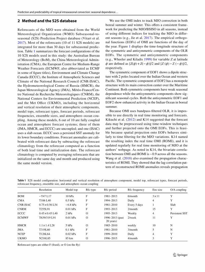
Reforecasts of the MJO were obtained from the World Meteorological Organization (WMO) Subseasonal-to-seasonal (S2S) Prediction Project database (Vitart et al. 2017). Most of the reforecasts (10 of 11 S2S models) are integrated for more than 30 days for subseasonal predic-tion. Table 1 summarizes the forecast configurations of the 10 S2S models used in this study: the Australian Bureau of Meteorology (BoM), the China Meteorological Admin-istration (CMA), the European Centre for Medium-Range Weather Forecasts (ECMWF, also abbreviated as ECMF in some of figure titles), Environment and Climate Change Canada (ECCC), the Institute of Atmospheric Sciences and Climate of the National Research Council (CNR-ISAC), the Hydrometeorological Centre of Russia (HMCR), the Japan Meteorological Agency (JMA), Météo-France/Cen-tre National de Recherche Meteorologiques (CNRM), the National Centers for Environmental Prediction (NCEP), and the Met Office (UKMO), including the horizontal and vertical resolution of their atmospheric components, model tops, reforecast types, forecast periods, reforecast frequencies, ensemble sizes, and atmosphere–ocean cou-pling. Among these models, 6 out of 10 are fully coupled ocean and atmosphere forecast systems; three of them (JMA, HMCR, and ECCC) are uncoupled; and one (ISAC) uses a slab ocean. ECCC uses a persisted SST anomaly for its lower boundary conditions. Forecast anomalies are cali-brated with reforecast data by subtracting the reforecast climatology from the reforecast computed as a function of both lead time and initialization date. The reforecast climatology is computed by averaging reforecasts that are initialized on the same day and month and produced using the same model version.

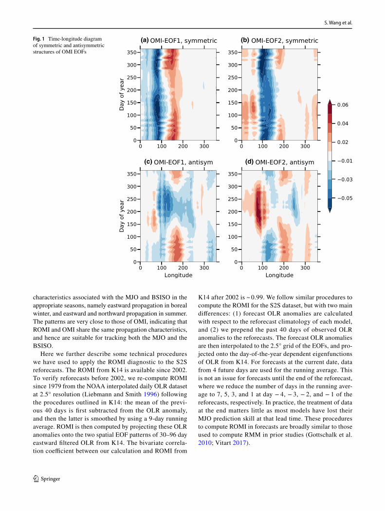
We use the OMI index to track MJO convection in both boreal summer and winter. This offers a consistent frame-work for predicting the MJO/BSISO in all seasons, instead of using different indices for tracking the MJO in differ-ent seasons (e.g., Jie et al. 2017). The empirical orthogo-nal functions (EOFs) of OMI are functions of the day of the year. Figure 1 displays the time-longitude structure of the symmetric and antisymmetric components of the OLR EOFs. The symmetric and antisymmetric components (e.g., Wheeler and Kiladis 1999) for variable Z at latitude ϕ are defined as [Z(ϕ) + Z(− ϕ)]/2 and [Z (ϕ) − Z (− ϕ)]/2, respectively.

The symmetric component of EOF1 shows a dipole struc-ture with 2 poles located over the Indian Ocean and western Pacific. The symmetric component of EOF2 has a monopole structure with its main convection center over the Maritime Continent. Both symmetric components have weak seasonal dependence while the antisymmetric components show sig-nificant seasonal cycles. Both the antisymmetric EOF1 and EOF2 show enhanced activity in the Indian Ocean in boreal summer.

Because OMI uses bandpass-filtered OLR, it is impos-sible to use directly in real time monitoring and forecasts. Kikuchi et al. (2012) and K14 suggested that the forecast data may be preprocessed using time-window techniques and further projected onto the OMI EOFs. This is feasi-ble because spatial projection onto EOFs behaves simi-larly to time filtering for the MJO variations. K14 named the resulting index the real time OMI (ROMI), and it is updated regularly for real time monitoring of MJO at the authors’ webpage. As noted in K14, the bivariate correla-tion between OMI and ROMI is ~ 0.9 across all the seasons. Wang et al. (2018) also examined the propagation charac-teristics of ROMI. They showed that the lag-correlation pat-tern of reconstructed ROMI anomalies reveals propagation

Table 1 S2S model configuration: horizontal and vertical resolution of atmosphere component, model top, reforecast types, forecast periods, reforecast frequency, ensemble size, and atmosphere–ocean coupling

Reforecast types are either F (fixed), or O (on the fly)

Resolution Model top Rfc type Rfc period Rfc frequency Ens size O/A coupling

BOM ~ T47 L17 10 hPa F 1981–2013 6/month 3 × 11 YCMA T106 L40 0.5 hPa F 1994–2013 Daily 4 YCNR-ISAC 0.75 × 0.56 L54 ~ 6.8 hPa F 1981–2010 Every 5 days 1 SlabCNRM T255L91 0.01 hPa F 1993–2013 2/month 15 YECCC 0.45 × 0.45 L40 2 hPa O 1995–2013 Weekly 4 Persistent SSTECMWF T639/319 L91 0.01 hPa O 1996–2013 (past

20 years)2/week 11 Y

HMCR 1.1 × 1.4 L28 5 hPa O 1985–2010 weekly 10 NJMA T319L60 0.1 hPa F 1981–2010 3/month 5 NNCEP T126L64 0.02 hPa F 1999–2010 Daily 4 YUKMO N216L85 85 km O 1996–2015 4/month 3 Y

S. Wang et al.

1 3

characteristics associated with the MJO and BSISO in the appropriate seasons, namely eastward propagation in boreal winter, and eastward and northward propagation in summer. The patterns are very close to those of OMI, indicating that ROMI and OMI share the same propagation characteristics, and hence are suitable for tracking both the MJO and the BSISO.

Here we further describe some technical procedures we have used to apply the ROMI diagnostic to the S2S reforecasts. The ROMI from K14 is available since 2002. To verify reforecasts before 2002, we re-compute ROMI since 1979 from the NOAA interpolated daily OLR dataset at 2.5° resolution (Liebmann and Smith 1996) following the procedures outlined in K14: the mean of the previ-ous 40 days is first subtracted from the OLR anomaly, and then the latter is smoothed by using a 9-day running average. ROMI is then computed by projecting these OLR anomalies onto the two spatial EOF patterns of 30–96 day eastward filtered OLR from K14. The bivariate correla-tion coefficient between our calculation and ROMI from

K14 after 2002 is ~ 0.99. We follow similar procedures to compute the ROMI for the S2S dataset, but with two main differences: (1) forecast OLR anomalies are calculated with respect to the reforecast climatology of each model, and (2) we prepend the past 40 days of observed OLR anomalies to the reforecasts. The forecast OLR anomalies are then interpolated to the 2.5° grid of the EOFs, and pro-jected onto the day-of-the-year dependent eigenfunctions of OLR from K14. For forecasts at the current date, data from 4 future days are used for the running average. This is not an issue for forecasts until the end of the reforecast, where we reduce the number of days in the running aver-age to 7, 5, 3, and 1 at day − 4, − 3, − 2, and − 1 of the reforecasts, respectively. In practice, the treatment of data at the end matters little as most models have lost their MJO prediction skill at that lead time. These procedures to compute ROMI in forecasts are broadly similar to those used to compute RMM in prior studies (Gottschalk et al. 2010; Vitart 2017).

Fig. 1 Time-longitude diagram of symmetric and antisymmetric structures of OMI EOFs

(a) (b)

(d)(c)

Prediction and predictability of tropical intraseasonal convection: seasonal dependence…

1 3

3 Results

3.1 Reforecast of a DYNAMO MJO event

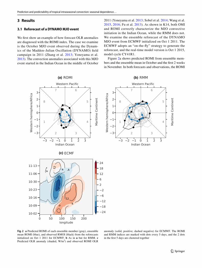
We first show an example of how forecast OLR anomalies are diagnosed with the ROMI index. The case we examine is the October MJO event observed during the Dynam-ics of the Madden–Julian Oscillation (DYNAMO) field campaign in 2011 (Zhang et al. 2013; Yoneyama et al. 2013). The convection anomalies associated with this MJO event started in the Indian Ocean in the middle of October

2011 (Yoneyama et al. 2013; Sobel et al. 2014; Wang et al. 2015, 2016; Fu et al. 2013). As shown in K14, both OMI and ROMI correctly characterize the MJO convective initiation in the Indian Ocean, while the RMM does not. We examine the ensemble reforecast of the DYNAMO MJO event from ECMWF initialized on Oct 1 2011. The ECMWF adopts an “on-the-fly” strategy to generate the reforecast, and the real-time model version is Oct 1 2015, model cycle CY41R1.

Figure 2a shows predicted ROMI from ensemble mem-bers and the ensemble mean in October and the first 2 weeks in November. In both forecasts and observations, the ROMI

(a)

(c)

(b)

Fig. 2 a Predicted ROMI of each ensemble member (gray), ensemble mean ROMI (blue), and observed RMOI (black) from the reforecasts initialized on Oct 1 2011 for ECMWF. b As in a but for RMM. c Predicted OLR anomaly (shaded, W/m2) and observed ROMI OLR

anomaly (solid, positive; dashed negative) for ECMWF. The ROMI and RMM indices are marked with dots every 5 days, and the 2 dots in the first 5 days are clustered together

S. Wang et al.

1 3

is in phases 7 and 8 in the first 10 days, indicating dry conditions over the Indian Ocean. ROMI grows out of the unit circle between Oct 10 and Oct 15 in both reforecasts and observations. In contrast, the predicted and observed RMM were both out of the unit circle in the western hemi-sphere (phases 8 and 1), and weakened in the Indian Ocean (Fig. 2b). RMM failed to capture the convective initiation of this MJO event, as other studies indicated (e.g., Ling et al. 2014). The reforecast predicted heightened MJO activity with the ROMI amplitude greater than 1 starting from mid-dle October, and weakened MJO activity in early November. This is very similar to what is seen in observations, despite ECMWF predicted ROMI amplitudes being notably weaker than observations from the start. As discussed later, underes-timation of MJO/BSISO amplitude is a common weakness in many S2S models. At the longer leads, the predicted ROMI index remains within the unit circle after early November. Hence it predicted that the MJO was unable to cross the Maritime Continent, contrary to observations.

The reconstructed OLR anomalies are derived from the predicted ROMI index and the eigenfunctions at cor-responding dates. Figure 2c shows that the model predicts well the eastward propagation of dry anomalies during the first 2 weeks of October and MJO convection initialization in the middle October. At longer leads, the predicted OLR anomalies experience difficulty sustaining eastward prop-agation out of the Indian Ocean and across the Maritime Continent, consistent with the impression obtained from the predicted ROMI index.

3.2 The correlation prediction skill and predictability

We assess the forecast skill of the ROMI index in the S2S models in this subsection using the bivariate correlation (e.g., Lin et al. 2008) for the reforecasts. Let F and O be forecast and observed ROMI index. F and O are vectors with two components ROMI1 and ROMI2: (F1, F2) and (O1, O2) for forecasts and observations, respectively. The bivariate correlation skill (COR) for the MJO index is written as:

where i denotes the index of the (re)forecasts. Here i < N, and N is the total number of forecasts. By construction, ROMI1 and ROMI2 are uncorrelated in observations, as they are projected onto two independent EOF patterns. In practice, this may not be entirely valid because the EOF patterns from the observations may not be strictly independent in the mod-els due to model biases. Nevertheless, our analysis of errors of ROMI1 and ROMI2 from the reforecasts indicate that the

(1)COR =

∑i Fi

⋅ Oi

�∑

i��Fi

��2

�∑

i��Oi

��2

errors are largely isotropic, suggesting that the assumption of orthogonality is approximately satisfied.

The bivariate correlation COR can be written explicitly in terms of the two components of the MJO index,

Errors in both amplitude and phase can contribute to degradation of the skill scores. Nevertheless, this form makes it difficult to separate the contributions of amplitude and phase to anomaly correlation skill. We rewrite the MJO indices in polar coordinates as F (f, θ), and O (o, φ), where f and o are amplitude, and θ and φ are phase angles for forecasts and observations, respectively. This allows us to write the bivariate correlation skill as:

This expression explicitly separates the contributions of amplitude and phase to ACC.

It is straightforward to consider several interesting lim-iting cases. If θ and φ differ by 90°, i.e., observations and forecasts are orthogonal, COR is 0. If there is no phase error, i.e., cos

(�i − �i

)= 1 , COR is the scalar amplitude

correlation:

If the amplitude is perfectly forecasted, i.e., the linear correlation between fi and oi is 1, COR is determined com-pletely by the relation between the forecast and observed phases, which is:

Both amplitude and phase correlations are higher than original bivariate correlation skill COR.

As an example, Fig. 3 shows the ROMI skill score and the corresponding amplitude and phase scores from the ECMWF model in boreal winter (model initialized from December to March) from 1999 to 2010. The ROMI cor-relation skill COR decreases below 0.5 after 43 days. Assuming perfect amplitude or phase forecasts results in improved correlation skill. Ignoring amplitude error results in overall slightly higher skill: CORp is slightly higher than COR by 0.05 at nearly all lead days. In contrast, taking out phase error leads to significantly higher skill: CORa is above 0.8 throughout the 45-day period. This result clearly

(2)COR =

∑i F1,iO1,i + F2,iO2,i

�∑i F1,i

2 + F2,i2

�∑i O1,i

2 + O2,i2

.

(3)COR =

∑i fi ⋅ oi ⋅ cos

��i − �i

�

�∑i fi

2�1∕2�∑

i oi2�1∕2 .

(4)CORa =

∑i fi ⋅ oi

�∑i fi

2�1∕2�∑

i oi2�1∕2 .

(5)CORp =

∑i oi

2⋅ cos

��i − �i

�

∑i oi

2.

Prediction and predictability of tropical intraseasonal convection: seasonal dependence…

1 3

demonstrates that elimination of phase errors would improve correlation more than elimination of amplitude errors would.

Figure 4 shows the ROMI bivariate correlation in boreal summer (June–September) and winter (December–March) for the 10 S2S models. All correlation skills are computed for ensemble mean forecasts except for ISAC, which is deter-ministic. Prediction skill measured by the number of days that COR exceeds 0.5 is 44 days for the ECMWF model in winter and 36 days in summer. The winter COR skill for ROMI exceeds the RMM forecast skill in Vitart (2017) by a few days. Other S2S models show less skill than does the ECMWF model. All the S2S models have lower fore-cast skill in summer than in winter by 3–10 days, and the difference is larger (~ more than 10 days) in NCEP/CFSv2 and BOM, and smaller (less than 5 days) in ECMWF and UKMO. The greater MJO convection prediction skill rep-resented by the ROMI than RMM is unexpected, since pre-vious studies have shown that convection prediction skill measured with the OLR component of the RMM index is less than that of the wind components. The relative lower RMM prediction skill is likely due to excessive noise inher-ent in RMM in comparison to bandpass filter based MJO indices, as noted by Ding et al. (2010), which further sug-gested that MJO prediction may be improved by using an index of inherently more predictable. Another important dis-tinction is that the RMM and OMI/ROMI differ significantly in their propagation characteristics in boreal summer (Wang et al. 2018). Therefore, the two indices are not measuring the same physical entities.

Predictability of these ensemble prediction systems is fur-ther assessed as the maximum number of forecast lead days at which signal variance equals the noise variance (T|SNR=1). The bivariate signal to noise ratio (SNR) is written as the ratio between variance of the ensemble forecast and total variance:

The signal and noise of the ensemble forecasts are esti-mated as:

where Xp denotes the ROMI index, and the subscript p indi-cates its two principal components. N and E denote the total number of forecasts and the number of ensemble members,

(6)SNR(�) =�2s

�2n

.

(7)�̂�2

s=

1

N − 1

N∑

n=1

2∑

p=1

(X̄np− X̄p

)2

,

(8)�̂�2

n=

1

N(E − 1)

N∑

n=1

E∑

m=1

2∑

p=1

(Xnmp

− X̄np

)2

,

Fig. 3 ROMI forecast skill from the ECMWF model for winter from 1999 to 2010 as a function of forecast leads (blue); ROMI forecast skill assuming perfect phase (COR_p, orange) and perfect amplitude (COR_p, red)

(a)

(b)

Fig. 4 a ROMI correlation skill score for COR = 0.5 and 0.6 in boreal winter (DJFM) and summer (JJAS). The dark and light colors corre-spond to prediction skill with threshold values 0.5 and 0.6, respec-tively. b Predictability measure as the time when SNR = 1. Models that have SNR less than 1 by the end of the forecasts are not shown

S. Wang et al.

1 3

respectively. X̄ is the overall mean, and X̄np denotes the

ensemble mean.SNR is greater than one at the longest lead forecast for

several models (NCEP, JMA, ECCC) in both seasons due to underdispersion. Figure 4b shows T|SNR=1 for the remain-ing six ensemble prediction models. All these models show greater predictability in winter than in summer, as does the COR measure. The difference of T|SNR=1 in both seasons varies, and does not necessarily reflect differences in COR in the two seasons. This seasonal dependence of tropical intra-seasonal predictability has been exposed before using the error growth measure in Ding et al. (2011), and our assess-ment of S2S prediction results is consistent with Ding et al.

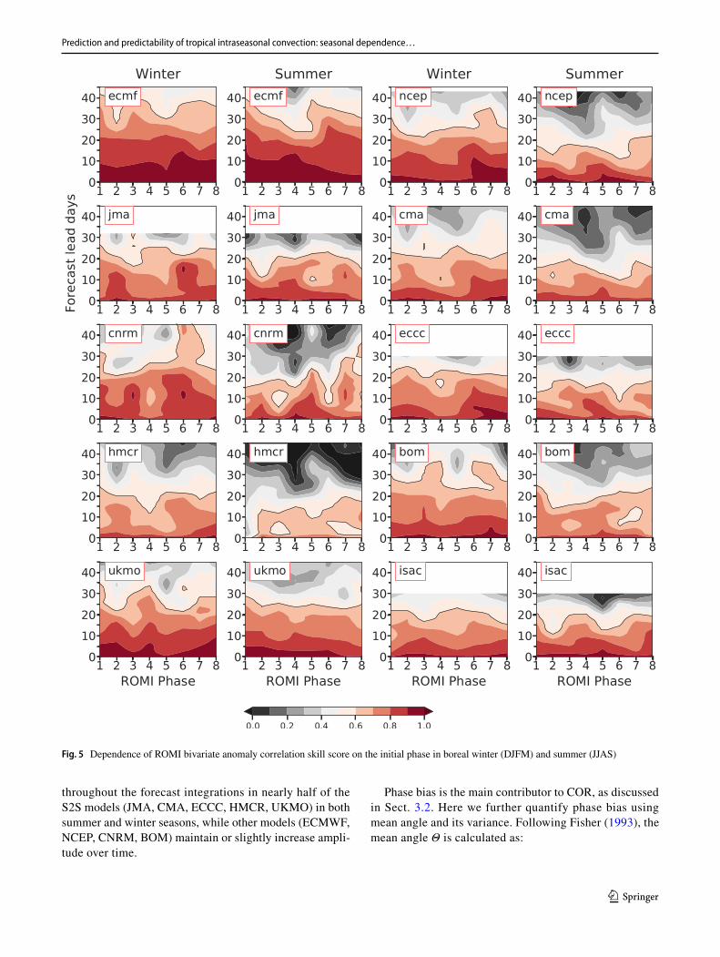
MJO prediction skill can be phase dependent. Here we examine the ROMI reforecast skill for MJO events with ini-tial amplitude greater than 1 in these S2S models (Fig. 5). Some models show better/worse skill in certain initial phases, e.g., lower COR in phases 2 and 5 in ECMWF in winter, and 4–5 in summer, higher skill winter phases 1 and 7 in NCEP. However, this initial phase dependence is mostly model dependent and not systematic. The same conclusion can be drawn for summer season prediction skill in the S2S models.

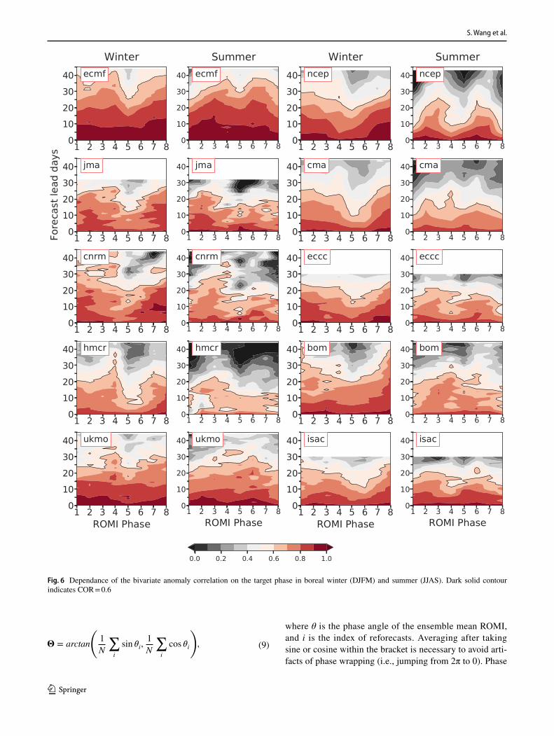
Systematic phase dependence of prediction skill is revealed when the correlation skill is composited upon the phase of the forecast target day. Figure 6 shows COR as a function of the target phases and forecast leads for target phase amplitudes greater than 1. Almost all models have lower bivariate correlation skills in phases 4–6 with a minimum in phase 5 in winter by 5–10 days in comparison to other phases, with the only exception being UKMO. During these phases MJO convection is centered in the Maritime Continent (MC). On the other hand, this prob-lem is not widespread in summer, though it does occur in NCEP, JMA and CNRM models; several models on the other hand show worse skill in phases 1 and 8, e.g., the ECMWF, CMA, ECCC, ISAC, HMCR models. Further examination of the MJO phase and amplitude correlations, CORa and CORp, reveals that the former has very similar target phase dependence as does COR, while CORp is rela-tively independent of target phase (not shown).

The difficulty of predicting MJO convection over the MC is sometimes called the MJO prediction barrier (Vitart and Molteni 2010). For example, Kim et al. (2016) dem-onstrated that the ECMWF model has difficulty in fore-casting convection anomalies at 10 days lead time, and the authors suggested that this issue arises in part due to deficiencies in using the RMM index to characterize MJO convection since Kelvin waves may be projected onto the RMM index. Here, the MJO MC prediction skill derived from the ROMI is greater in general than what was found by Kim et al. (2016), and the barrier is manifest in the S2S

models’ deficiency in predicting the peak phases of MJO convection over the MC.

3.3 Composites of OLR anomalies

The ROMI OLR prediction skills are higher than grid-point OLR prediction skills in some of the S2S models (e.g., Weber and Mass 2017; Janiga et al. 2018). The ROMI prediction skills are better than the RMM prediction skills in the same S2S models in boreal winter (Fig. 1 of Vitart 2017). For example, ECMWF exhibits 34 day prediction skill in ROMI using COR = 0.6, as compared to 28-day skill in RMM; the HMCR model exhibits ~ 21-day skill in ROMI, but only 6-day skill in RMM. It is unexpected that the MJO convection prediction skill (ROMI) is higher than the MJO circulation prediction skill (RMM), as this is opposite to what prior studies have shown by comparing the skill of the circulation and convection components of RMM separately. One reason for this index dependence might be that the convection component of RMM is not optimized for MJO convection to achieve maximum intraseasonal variance and predictability. Lag correlation between the two components of RMM is much lower than that in ROMI (e.g., e.g., Wang et al. 2018), indicating that ROMI is better at extracting propagating signals.

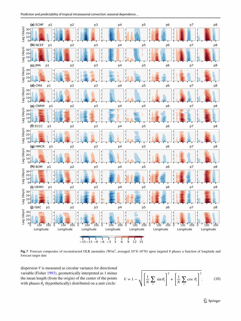
To see that this ROMI skill bears some physical mean-ing, we composite the reconstructed ROMI OLR anomalies from the S2S models. Composites of the OLR anomalies are constructed as a function of longitude and forecast lead for the observed MJO phases defined using ROMI at the forecast target lead (Fig. 7). The OLR anomalies at day 0 are each model’s forecast at day 0, and are very close to observations. At longer days, the forecasted OLR anomalies deviate from the initial values in two ways: decreases in amplitude and errors of either sign in phase. For example, the reconstructed OLR anomaly from ECMWF in phase 5, with convection located at the MC (100–140 E), weakens substantially by day 20, more so than do OLR anomalies in other phases. The NCEP OLR anomaly in phase 5 is notably shifted westward by ~ 10°, as a result of too slow propaga-tion. Overall, the composite anomaly is consistent with the phase dependent prediction skill in Fig. 6.

3.4 Further assessment of amplitude and phase bias

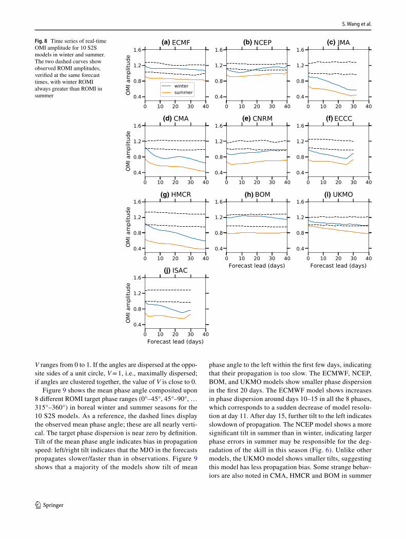
The bivariate correlation skill measures linear correlation between observations and forecasts. It is independent of systematic amplitude bias. The latter is considered in this subsection. Composite of the ensemble mean ROMI ampli-tude as a function of forecast leads (Fig. 8) indicates that most S2S models underestimate ROMI amplitude in the first day (except UKMO). This bias in amplitude amplifies

Prediction and predictability of tropical intraseasonal convection: seasonal dependence…

1 3

throughout the forecast integrations in nearly half of the S2S models (JMA, CMA, ECCC, HMCR, UKMO) in both summer and winter seasons, while other models (ECMWF, NCEP, CNRM, BOM) maintain or slightly increase ampli-tude over time.

Phase bias is the main contributor to COR, as discussed in Sect. 3.2. Here we further quantify phase bias using mean angle and its variance. Following Fisher (1993), the mean angle Θ is calculated as:

Fig. 5 Dependence of ROMI bivariate anomaly correlation skill score on the initial phase in boreal winter (DJFM) and summer (JJAS)

S. Wang et al.

1 3

(9)� = arctan

(1

N

∑

i

sin �i,1

N

∑

i

cos �i

)

,

where θ is the phase angle of the ensemble mean ROMI, and i is the index of reforecasts. Averaging after taking sine or cosine within the bracket is necessary to avoid arti-facts of phase wrapping (i.e., jumping from 2π to 0). Phase

Fig. 6 Dependance of the bivariate anomaly correlation on the target phase in boreal winter (DJFM) and summer (JJAS). Dark solid contour indicates COR = 0.6

Prediction and predictability of tropical intraseasonal convection: seasonal dependence…

1 3

dispersion V is measured as circular variance for directional variable (Fisher 1993), geometrically interpreted as 1 minus the mean length (from the origin) of the center of the points with phases �k (hypothetically) distributed on a unit circle:

(10)V = 1 −

√√√√√

[1

N

∑

i

sin �i

]2

+

[1

N

∑

i

cos �i

]2

.

(a)

(b)

(c)

(d)

(e)

(f)

(g)

(h)

(i)

(j)

Fig. 7 Forecast composites of reconstructed OLR anomalies (W/m2, averaged 10°S–10°N) upon targeted 8 phases a function of longitude and forecast target date

S. Wang et al.

1 3

V ranges from 0 to 1. If the angles are dispersed at the oppo-site sides of a unit circle, V = 1, i.e., maximally dispersed; if angles are clustered together, the value of V is close to 0.

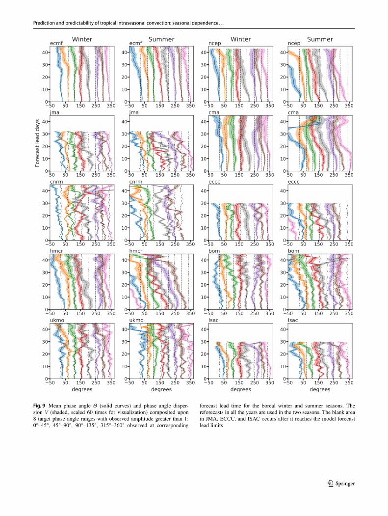
Figure 9 shows the mean phase angle composited upon 8 different ROMI target phase ranges (0°–45°, 45°–90°, … 315°–360°) in boreal winter and summer seasons for the 10 S2S models. As a reference, the dashed lines display the observed mean phase angle; these are all nearly verti-cal. The target phase dispersion is near zero by definition. Tilt of the mean phase angle indicates bias in propagation speed: left/right tilt indicates that the MJO in the forecasts propagates slower/faster than in observations. Figure 9 shows that a majority of the models show tilt of mean

phase angle to the left within the first few days, indicating that their propagation is too slow. The ECMWF, NCEP, BOM, and UKMO models show smaller phase dispersion in the first 20 days. The ECMWF model shows increases in phase dispersion around days 10–15 in all the 8 phases, which corresponds to a sudden decrease of model resolu-tion at day 11. After day 15, further tilt to the left indicates slowdown of propagation. The NCEP model shows a more significant tilt in summer than in winter, indicating larger phase errors in summer may be responsible for the deg-radation of the skill in this season (Fig. 6). Unlike other models, the UKMO model shows smaller tilts, suggesting this model has less propagation bias. Some strange behav-iors are also noted in CMA, HMCR and BOM in summer

Fig. 8 Time series of real-time OMI amplitude for 10 S2S models in winter and summer. The two dashed curves show observed ROMI amplitudes, verified at the same forecast times, with winter ROMI always greater than ROMI in summer

(a) (b) (c)

(d)

(g)

(j)

(h) (i)

(e) (f)

Prediction and predictability of tropical intraseasonal convection: seasonal dependence…

1 3

Fig. 9 Mean phase angle Θ (solid curves) and phase angle disper-sion V (shaded, scaled 60 times for visualization) composited upon 8 target phase angle ranges with observed amplitude greater than 1: 0°–45°, 45°–90°, 90°–135°, 315°–360° observed at corresponding

forecast lead time for the boreal winter and summer seasons. The reforecasts in all the years are used in the two seasons. The blank area in JMA, ECCC, and ISAC occurs after it reaches the model forecast lead limits

S. Wang et al.

1 3

after day 30 days as a result of loss of predictability for ROMI at this long lead.

3.5 Probabilistic prediction of ROMI

Most of the S2S modeling groups adopt ensemble-based probabilistic forecast approaches. The number of ensemble members varies from 3 (e.g., UKMO) to 33 (e.g., BOM). The correlation skill is a measure of the ensemble mean skill without consideration of ensemble spread. Here we estimate the probabilistic prediction skill in the S2S reforecasts for 9 ensemble forecasts. We use the ranked probability skill score (RPSS) to quantify probabilistic ROMI prediction skills of the MJO amplitude (e.g., Marshall et al. 2016). RPSS is an extension of the Brier Skill Score to scoring forecasts of ordered multiple-category events. Following the notation in Wilks (2011), Ranked Probability Score (RPS) is defined for each ensemble forecast as:

RPS =

C∑

m=1

(Ym − Om

)2,

where C is the number of categories, Ym and Om are the cumulative probabilistic distributions of forecasts and obser-vations, respectively. RPSS for multiple forecasts is then:

where the overbar denotes an average over multiple fore-casts, and RPSclim denotes RPS for climatology. We use C = 10 categories for ROMI: < 0.25, 0.25–0.5, 0.5–0.75, 0.75–1, 1–1.25, 1.25–1.5, 1.5–1.75, 1.75–2, 2–3, > 3. These categories will be used to evaluate ROMI amplitude.

RPSS is a relative forecast skill score and depends on the choice of climatological reference forecast. We have tested different choices of RPSclim , and we found that a reasonable choice of RPSclim is to construct an observa-tion ensemble with 20 ensemble members taken from 20 years’ observations on the same day of the year. A prob-abilistic forecast is skillful if RPS exceeds RPSclim i.e., RPSS is greater than 0. As shown below, some models have no RPSS skill from day 0. This value of the RPSS skill may not be directly comparable to the correlation

RPSS = 1 −RPS

RPSclim

Fig. 10 Top panels: RPSS for the ROMI forecasts as a func-tion of lead days in boreal win-ter and summer. Solid/dashed curves indicate the model have more/less than 10 ensemble members. The bottom panels are similar to top panels, except that the systematic amplitude bias (in Fig. 8) is corrected

(b)(a)

(c) (d)

Prediction and predictability of tropical intraseasonal convection: seasonal dependence…

1 3

skill discussed in previous sections, since RPSS is sensi-tive to systematic bias while correlation is not.

Figure 10a shows RPSS of ROMI amplitude in winter from 1999 to 2010. ECMF and BOM are skillful at fore-cast leads of more than 30 days. UKMO and NCEP are skillful at forecast leads of more than 10 days. The rest of the models are skillful at forecast lead less than 10 days. Figure 10b shows RPSS for summer. Overall the RPSS skills of these 9 S2S models are less skillful in summer than in winter. This seasonal dependence is consistent with the deterministic skill discussed in the previous sec-tion. The lack of probabilistic skill in some of these mod-els may be attributed to their systematic underestimates of amplitude (Fig. 8). Since this systematic bias is known, we may add back the known bias as function of forecast lead (Fig. 8) to improve RPSS. Figure 10c, d show that the RPSS skill improves for all the models when this is done, such that all the models exhibit RPSS skill at lead times greater than 5 days in winter.

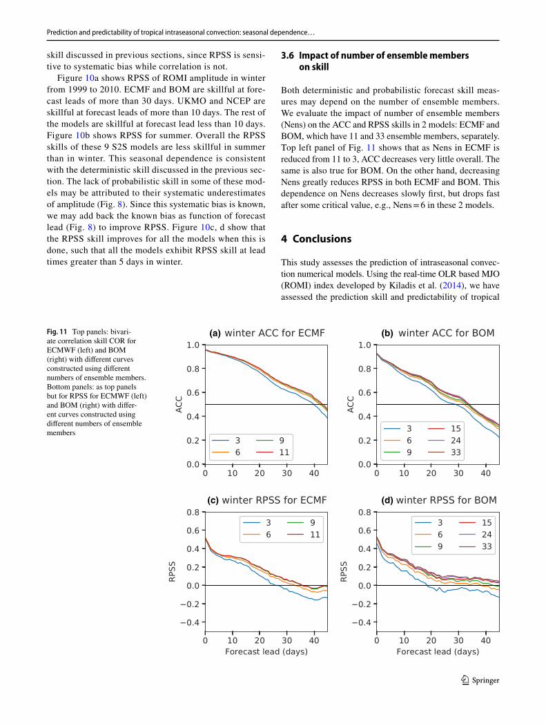
3.6 Impact of number of ensemble members on skill

Both deterministic and probabilistic forecast skill meas-ures may depend on the number of ensemble members. We evaluate the impact of number of ensemble members (Nens) on the ACC and RPSS skills in 2 models: ECMF and BOM, which have 11 and 33 ensemble members, separately. Top left panel of Fig. 11 shows that as Nens in ECMF is reduced from 11 to 3, ACC decreases very little overall. The same is also true for BOM. On the other hand, decreasing Nens greatly reduces RPSS in both ECMF and BOM. This dependence on Nens decreases slowly first, but drops fast after some critical value, e.g., Nens = 6 in these 2 models.

4 Conclusions

This study assesses the prediction of intraseasonal convec-tion numerical models. Using the real-time OLR based MJO (ROMI) index developed by Kiladis et al. (2014), we have assessed the prediction skill and predictability of tropical

Fig. 11 Top panels: bivari-ate correlation skill COR for ECMWF (left) and BOM (right) with different curves constructed using different numbers of ensemble members. Bottom panels: as top panels but for RPSS for ECMWF (left) and BOM (right) with differ-ent curves constructed using different numbers of ensemble members

(a) (b)

(c) (d)

S. Wang et al.

1 3

intraseasonal convection anomalies in the WMO subseasonal to seasonal (S2S) forecast database. The main conclusions are:

1. The ROMI prediction skills, measured by bivariate correlation coefficient exceeding 0.6, range from ~ 15 to ~ 36 days in boreal winter in the S2S models. This range is 5–10 days higher than that derived from the MJO RMM index in several prior studies. Forecasts of the BSISO have systematically lower skill than those of the MJO by 5–10 days. These results suggest that intraseasonal convection is inherently less predictable in summer than in winter. Analysis of an additional pre-dictability measure, signal to noise ratio, confirms this seasonal dependence.

2. Further evaluation of the bivariate correlation skill, assuming either perfect amplitude or perfect phase fore-casts, indicates that phase bias is the main contributor to skill degradation at longer lead times. A new diagnos-tic—phase dispersion—is developed to represent depar-ture of phase speed from observation. The S2S models show phase dispersion varies by target phases. Assess-ment of the ROMI amplitude indicates that many S2S models significantly underestimate ROMI amplitudes at longer forecast leads.

3. Composites of MJO convection prediction skill upon target phases show that nearly all the S2S models have less skill when the MJO convection is centered over the Maritime Continent (MC) in boreal winter at the target date, and that phase bias contributes to this MC predic-tion barrier. There is no consistent dependence of skill on initial phase across the multi-model ensemble. This issue is less prevalent in boreal summer. It is unclear what processes are responsible for the lack of skill in the MC region. This issue will be explored in the future.

4. Probabilistic evaluation of the S2S model skills in fore-casting ROMI amplitude indicates that ranked probabil-ity skill scores are significantly degraded in many mod-els due to amplitude bias. Accounting for this systematic bias in prior leads to improvement in RPSS.

Acknowledgements This research has been conducted as part of the NOAA MAPP S2S Prediction Task Force and supported by NOAA Grant NA16OAR4310076. SW and AHS also acknowledge support from NSF AGS-1543932 and ONR N00014-16-1-3073. We are grate-ful for the insightful comments by three anomalous reviewers. We thank Haibo Liu for obtaining and organizing the S2S data set from the ECMWF data portal.

References

Baggett CF, Barnes EA, Maloney ED, Mundhenk BD (2017) Advanc-ing atmospheric river forecasts into subseasonal-to-seasonal time scales. Geophys Res Lett 44:7528–7536

Ding RQ, Li JP, Seo K (2010) Predictability of the Madden–Julian oscillation estimated using observational data. Mon Wea Rev 138:1004–1013. https ://doi.org/10.1175/2009M WR308 2.1

Ding RQ, Li JP, Seo K (2011) Estimate of the predictability of boreal summer and winter intraseasonal oscillations from observations. Mon Wea Rev 139:2421–2438. https ://doi.org/10.1175/2011M WR357 1.1

Fisher NI (1993) Statistical analysis of circular data. Cambridge University Press, Cambridge, p 277

Fu X, Lee JY, Hsu PC et al (2013) Multi-model MJO forecasting during DYNAMO/CINDY period. Clim Dyn 41:1067–1081

Gottschalk J, Wheeler M, Weickmann K, Vitart F, Savage N, Lin H, Hendon H, Waliser D, Sperber K, Prestrelo C, Nakagawa M, Flatau M, Higgins W (2010) A framework for assessing operational model MJO forecasts: a project of the CLIVAR Madden–Julian oscillation Working Group. Bull Am Meteorol Soc 91:1247–1258

Hoskins BJ (2013) The potential for skill across the range of the seam-less weather-climate prediction problem: a stimulus for our sci-ence. Q J R Meteorol Soc 139:573–584. https ://doi.org/10.1002/qj.1991

Janiga MA, Schreck CJ, Ridout JA, Flatau M, Barton NP, Metzger EJ, Reynolds CA (2018) Subseasonal forecasts of convectively coupled equatorial waves and the MJO: activity and predictive skill. Mon Wea Rev 146:2337–2360. https ://doi.org/10.1175/MWR-D-17-0261.1

Jiang X, Waliser DE, Wheeler MC, Jones C, Lee M, Schubert SD (2008) Assessing the skill of an all-season statistical fore-cast model for the Madden–Julian oscillation. Mon Wea Rev 136:1940–1956. https ://doi.org/10.1175/2007M WR230 5.1

Jie W, Vitart F, Wu T, Liu X (2017) Simulations of Asian Summer monsoon in the sub-seasonal to seasonal prediction project (S2S) database. Q J R Meterol Soc. https ://doi.org/10.1002/qj.3085

Jones C, Waliser DE, Lau KM, Stern W (2004) Global occurrences of extreme precipitation and the Madden–Julian oscillation: obser-vations and predictability. J Clim 17:4575–4589. https ://doi.org/10.1175/3238.1

Kang I, Kim H (2010) Assessment of MJO predictability for boreal winter with various statistical and dynamical models. J Clim 23:2368–2378. https ://doi.org/10.1175/2010J CLI32 88.1

Kikuchi K, Wang B, Kajikawa Y (2012) Bimodal representation of the tropical intraseasonal oscillation. Clim Dyn 38:1989–2000. https ://doi.org/10.1007/s0038 2-011-1159-1

Kiladis GN, Dias J, Straub KH, Wheeler MC, Tulich SN, Kikuchi K, Weickmann KM, Ventrice MJ (2014) A comparison of OLR and circulation-based indices for tracking the MJO. Mon Wea Rev 142:1697–1715. https ://doi.org/10.1175/MWR-D-13-00301 .1

Kim H, Webster PJ, Toma VE, Kim D (2014) Predictability and pre-diction skill of the MJO in two operational forecasting systems. J Clim 27:5364–5378. https ://doi.org/10.1175/JCLI-D-13-00480 .1

Kim H, Kim D, Vitart F, Toma VE, Kug J, Webster PJ (2016) MJO propagation across the Maritime Continent in the ECMWF ensemble prediction system. J Clim 29:3973–3988. https ://doi.org/10.1175/JCLI-D-15-0862.1

Klingaman NP et al (2015) Vertical structure and physical processes of the Madden–Julian oscillation: linking hindcast fidelity to sim-ulated diabatic heating and moistening. J Geophys Res Atmos 120:4690–4717. https ://doi.org/10.1002/2014J D0223 74

Krishnamurti TN, Subramanian D (1982) The 30–50 day mode at 850 mb during MONEX. J Atmos Sci 39:2088–2095

Lee JY, Wang B, Wheeler MC, Fu X, Waliser DE, Kang I-S (2013) Real-time multivariate indices for the boreal summer intraseasonal oscillation over the Asian summer monsoon region. Clim Dyn 40:493–509. https ://doi.org/10.1007/s0038 2-012-1544-4

Li T, Wang L, Peng M, Wang B, Zhang C, Lau W, Kuo H (2018) A paper on the tropical intraseasonal oscillation published in 1963

Prediction and predictability of tropical intraseasonal convection: seasonal dependence…

1 3

in a Chinese journal. Bull Am Meteor Soc 99:1765–1779. https ://doi.org/10.1175/BAMS-D-17-0216.1

Liebmann B, Smith CA (1996) Description of a complete (interpo-lated) outgoing long-wave radiation dataset. Bull Am Meteor Soc 77:1275–1277

Lim Y, Son S, Kim D (2018) MJO prediction skill of the subseasonal-to-seasonal prediction models. J Clim 31:4075–4094. https ://doi.org/10.1175/JCLI-D-17-0545.1

Lin H, Brunet G, Derome J (2008) Forecast skill of the Madden–Julian oscillation in two Canadian atmospheric models. Mon Wea Rev 136:4130–4149. https ://doi.org/10.1175/2008M WR245 9.1

Lin H, Brunet G, Derome J (2009) An observed connection between the North Atlantic oscillation and the Madden–Julian oscillation. J Clim 22:364–380. https ://doi.org/10.1175/2008J CLI25 15.1

Ling J, Bauer P, Bechtold P, Beljaars A, Forbes R, Vitart F, Ulate M, Zhang C (2014) Global versus local MJO forecast skill of the ECMWF Model during DYNAMO. Mon Wea Rev 142:2228–2247. https ://doi.org/10.1175/MWR-D-13-00292 .1

Madden RA, Julian PR (1971) Detection of a 40–50 day oscillation in the zonal wind in the tropical Pacific. J Atmos Sci 28:702–708

Madden RA, Julian PR (1972) Description of global-scale circula-tion cells in the tropics with a 40–50 day period. J Atmos Sci 29:1109–1122

Marshall AG, Hendon HH, Hudson D (2016), Visualizing and verify-ing probabilistic forecasts of the Madden-Julian oscillation, Geo-phys Res Lett 43:12,278–12,286. https ://doi.org/10.1002/2016G L0714 23

Neena JM, Lee JY, Waliser D, Wang B, Jiang X (2014) Predictability of the Madden–Julian oscillation in the intraseasonal variability hindcast experiment (ISVHE). J Clim 27:4531–4543. https ://doi.org/10.1175/JCLI-D-13-00624 .1

Rashid HA, Hendon HH, Wheeler MC, Alves O (2011) Prediction of the Madden–Julian oscillation with the POAMA dynamical prediction system. Clim Dyn 36:649–661

Robertson AW, Kuma A, Peña M, Vitart F (2015) Improving and pro-moting subseasonal to seasonal prediction. Bull Am Meteor Soc 96:ES49–ES53

Sobel AH, Wang S, Kim D (2014) Moist static energy budget of the MJO during DYNAMO. J Atmos Sci 71:4276–4291

Straub KH (2013) MJO initiation in the real-time multivariate MJO index. J Clim 26:1130–1151. https ://doi.org/10.1175/JCLI-D-12-00074 .1

Ventrice MJ, Wheeler MC, Hendon HH, Schreck CJ, Thorncroft CD, Kiladis GN (2013) A modified multivariate Madden–Julian oscil-lation index using velocity potential. Mon Wea Rev 141:4197–4210. https ://doi.org/10.1175/MWR-D-12-00327 .1

Vitart F (2014) Evolution of ECMWF sub-seasonal forecast skill scores. Q J R Meteorol Soc 140:1889–1899

Vitart F (2017) Madden—Julian oscillation prediction and telecon-nections in the S2S database. QJR Meteorol Soc 143:2210–2220. https ://doi.org/10.1002/qj.3079

Vitart F, Molteni F (2010) Simulation of the MJO and its telecon-nections in the ECMWF forecast system. Q J R Meteorol Soc 136:842–855

Vitart F et al (2017) The subseasonal to seasonal (S2S) prediction project database. Bull Amer Meteor Soc 98:163–173. https ://doi.org/10.1175/BAMS-D-16-0017.1

Waliser DE, Lau KM, Stern W, Jones C (2003) Potential predictability of the Madden–Julian oscillation. Bull Amer Meteor Soc 84:33–50. https ://doi.org/10.1175/BAMS-84-1-33

Wang W, Hung MP, Weaver SJ, Kumar A, Fu X (2014) MJO predic-tion in the NCEP climate forecast system version 2. Clim Dyn 42:2509–2520

Wang S, Sobel AH, Zhang F, Sun Q, Yue Y, Zhou L (2015) Regional simulation of the october and november MJO events observed dur-ing the CINDY/DYNAMO field campaign at gray zone resolution. J Clim 28:2097–2119

Wang S, Sobel AH, Nie J (2016) Modeling the MJO in a cloud-resolv-ing model with parameterized large-scale dynamics: Vertical structure, radiation, and horizontal advection of dry air. J Adv Model Earth Syst. https ://doi.org/10.1002/2015M S0005 29

Wang S, Anichowski A, Tippett M, Sobel A (2017) Seasonal noise vs. subseasonal signal: forecasts of California precipitation during the unusual winters of 2015–16 and 2016–17. Geophys Res Lett. https ://doi.org/10.1002/2017G L0750 52

Wang S, Ma D, Sobel AH, Tippett MK (2018) Propagation char-acteristics of BSISO indices. Geophys Res Lett.  https ://doi.org/10.1029/2018G L0783 21

Weber NJ, Mass CF (2017) Evaluating CFSv2 subseasonal forecast skill with an emphasis on tropical convection. Mon Wea Rev 145:3795–3815. https ://doi.org/10.1175/MWR-D-17-0109.1

Wheeler M, Kiladis GN (1999) Convectively coupled equatorial waves: analysis of clouds and temperature in the wavenumber–frequency domain. J Atmos Sci 56:374–399

Wheeler MC, Hendon HH (2004) An all-season real-time multivariate MJO index: Development of an index for monitoring and predic-tion. Mon Wea Rev 132:1917–1932

Wilks DS (2011) Statistical methods in the atmospheric sciences, 3rd edn. Academic, San Diego

Wu J, Ren HL, Zuo JQ et al (2016) MJO prediction skill, predictability, and teleconnection impacts in the Beijing Climate Center Atmos-pheric General Circulation Model. Dyn Atmos Oceans 75:78–90. https ://doi.org/10.1016/j.dynat moce.2016.06.001

Xiang B, Zhao M, Jiang X et al (2015) The 3–4-week MJO prediction skill in a GFDL coupled model. J Clim 28:5351–5364

Xie YB, Chen SJ, Zhang IL, Hung YL (1963) A preliminarily statistic and synoptic study about the basic currents over southeastern Asia and the initiation of typhoon. Acta Meteorol Sin 33(2):206–217

Yasunari T (1979) Cloudiness fluctuations associated with the northern hemisphere summer monsoon. J Meteorol Soc Jpn 57:227–242

Yoneyama K, Zhang C, Long CN (2013) Tracking pulses of the Mad-den-Julian oscillation. Bull Am Meteorol Soc 94:1871–1891. https ://doi.org/10.1175/BAMS-D-12-00157 .1

Zhang C (2013) Madden–Julian oscillation: bridging weather and climate. Bull Am Meteor Soc 94:1849–1870. https ://doi.org/10.1175/BAMS-D-12-00026 .1

Zhang C, Gottschalck J, Maloney ED, Moncrieff M, Vitart F, Wal-iser DE et al (2013) Cracking the MJO nut. Geophys Res Lett 40:1223–1230. https ://doi.org/10.1002/grl.50244