Predicting the outcomes of treatment to eradicate the ... · Predicting the outcomes of treatment...

Predicting the outcomes of treatment to eradicate thelatent reservoir for HIV-1

Alison L. Hill1,2,*, Daniel I. S. Rosenbloom1,3,*, Feng Fu4, Martin A. Nowak1,and Robert F. Siliciano5

1Program for Evolutionary Dynamics, Department of Mathematics, Department of Organismic andEvolutionary Biology, Harvard University, Cambridge, MA 02138, USA

2Biophysics Program and Harvard-MIT Division of Health Sciences and Technology, Harvard University,Cambridge, MA 02138, USA

3Department of Biomedical Informatics, Columbia University Medical Center, New York, NY 10032, USA4Institute of Integrative Biology, ETH Zurich, 8092 Zurich, Switzerland

5Department of Medicine, Johns Hopkins University School of Medicine, and Howard Hughes MedicalInstitute, Baltimore, MD 21205, USA

*These authors contributed equally to the manuscript

March 18, 2014

Abstract

Massive research efforts are now underway to develop a cure for HIV infection, allow-ing patients to discontinue lifelong combination antiretroviral therapy (ART). New latency-reversing agents (LRAs) may be able to purge the persistent reservoir of latent virus in restingmemory CD4+ T cells, but the degree of reservoir reduction needed for cure remains un-known. Here we use a stochastic model of infection dynamics to estimate the efficacy ofLRA needed to prevent viral rebound after ART interruption. We incorporate clinical datato estimate population-level parameter distributions and outcomes. Our findings suggest thatapproximately 2,000-fold reductions are required to permit a majority of patients to interruptART for one year without rebound and that rebound may occur suddenly after multiple years.Greater than 10,000-fold reductions may be required to prevent rebound altogether. Our re-sults predict large variation in rebound times following LRA therapy, which will complicateclinical management. This model provides benchmarks for moving LRAs from the lab to theclinic and can aid in the design and interpretation of clinical trials. These results also applyto other interventions to reduce the latent reservoir and explain the observed return of viremiaafter months of apparent cure in recent bone marrow transplant recipients.

1

arX

iv:1

403.

4196

v1 [

q-bi

o.PE

] 1

7 M

ar 2

014

IntroductionThe latent reservoir (LR) for HIV-1 is a population of long-lived resting memory CD4+ T cells withintegrated HIV-1 DNA1. After establishment during acute infection2, it increases to 105−107 cellsand then remains stable. As only replicating virus is targeted by antiretroviral therapy (ART), la-tently infected cells persist even after years of effective treatment3–7. Cellular activation leads tovirus production and, if treatment is interrupted, viremia rebounds within weeks8;9. Several molec-ular mechanisms maintain latency, including epigenetic modifications, transcriptional interferencefrom host genes, and the absence of activated transcription factors10–13.

Major efforts are underway to identify pharmacologic agents that reverse latency by trigger-ing the expression of HIV-1 genes in latently infected cells, with the hope that cell death fromviral cytopathic effects or cytolytic immune responses follows, reducing the size of the LR14;15.Collectively called latency-reversing agents (LRAs), these drugs include histone deacetylase in-hibitors16–18, protein kinase C activators19–22, and the bromodomain inhibitor JQ123–25. WhileLRAs are the subject of intense research, it is unclear how much the LR must be reduced to enablepatients to safely discontinue ART.

The feasibility of reservoir reduction as a method of HIV-1 cure is supported by case studies ofstem-cell transplantation26;27 and, more recently, early treatment initiation28;29, which have allowedpatients to interrupt treatment for months or years without viral rebound. The dramatic reductionsin reservoir size accompanying these strategies stands in stark contrast to the actions of currentLRAs, which induce only a fraction of latent virus in vitro30;31 and have not produced a measurabledecrease in LR size in vivo16;17;32. It unclear how patient outcomes depend on reservoir reductionbetween these extremes, nor even whether a reduction that falls short of those achieved with stem-cell transplantation will bring any clinical benefit. LRA research needs to address the question:how low must we go?

In the absence of clinical data, mechanistic mathematical models can serve as a framework topredict results of novel interventions and plan clinical trials. When results do become available,the models can be tested and refined. Mathematical models have a long tradition of informingHIV-1 research and have been particularly useful in understanding HIV-1 treatment. Previousmodels have explained the multi-phasic decay of viremia during antiretroviral therapy33;34, the ini-tial seeding of the LR during acute infection35, the limited inflow to the LR during treatment36, thedynamics of viral blips37, and the contributions of the LR to drug resistance38. No model has yetbeen offered to describe the effect of LRAs. Here we present a novel modeling framework to pre-dict the degree of reservoir reduction needed to prevent viral rebound following ART interruption.The model can be used to estimate the probability that cure is achieved, or, barring that outcome,to estimate the length of time following treatment interruption before viral rebound occurs (Fig.1a).

2

Cells remaining in LR Dynamics of each cell

NLR q NLR

Initial LR size

LRA ART

-3 -2 -1 0 1 210-6

10-4

10-2

1

Time since treatment interruption (years)

LR s

ize

(vs.

orig

inal

)

Rebound?

Clearance?

-3 -2 -1 0 1 2

104

10-2

102

1

Pla

sma

HIV

-1 R

NA

(co

pies

/ml)

Rebound time

Residual viremia

200 c/ml

Rebound?

Clearance?

b

a

Figure 1: Schematic of treatment with latency-reversing agents (LRA) and stochastic model of reboundfollowing interruption of ART. a) Proposed treatment protocol, illustrating possible viral load and size of LRbefore and after LRA therapy. When ART is started, viral load decreases rapidly and may fall below the limitof detection. The LR is established early in infection (not shown) and decays very slowly over time. WhenLRA is administered (either continuously, as shown, or in intervals), the LR declines. After discontinuationof ART, the infection may be cleared, or viremia may eventually rebound. b) LRA efficacy is defined bythe parameter q, the fraction of the LR remaining after therapy, which determines the initial conditions ofthe model. The stochastic model of viral dynamics following interruption of ART and LRA tracks bothlatently infected resting CD4+ T cells (rectangles) and productively infected CD4+ T cells (ovals). Eacharrow represents an event that occurs in the model. Alternate models considering homeostatic proliferationand turnover of the LR are discussed in the Methods and Supplementary Methods. Viral rebound occurs ifat least one remaining cell survives long enough to activate and produce a chain of infection events leadingto detectable infection (plasma HIV-1 RNA > 200 c ml−1).

3

Results

Determination of key viral dynamic parameters governing patient outcomesWe employ a stochastic model of HIV-1 reservoir dynamics and rebound that, in its simplest form,tracks two cell types: productively infected activated CD4+ T cells and latently infected restingCD4+ T cells (Fig. 1b). A latently infected cell can either activate or die, each with a particular rateconstant. An actively infected cell can produce a burst of virions, resulting in the active infectionof some number of other cells, or it can die from other causes without producing virions that infectother cells. The model only tracks the initial stages of viral rebound, when target cells are not yetlimited. This model is similar to other stochastic models of viral dynamics39, and a full descriptionis provided in the Methods and Supplementary Methods. The initial conditions for the dynamicmodel depend on the number of latently infected cells remaining following LRA therapy. LRAefficacy is defined by the fraction q of the LR that remains following therapy. The model trackseach latent and active cell to determine whether viral rebound occurs, and if so, how long it takes.Importantly, no single activated cell is guaranteed to re-establish the infection, as it may die prior toinfecting other cells. Even if it does infect others, those cells likewise may die prior to completingfurther infection. This possibility is a general property of stochastic models, and the specific valuefor the “establishment probability” depends on the rates at which infection and death events occur.Our goal is to calculate the probability that at least one of the infected cells remaining after therapyescapes extinction and causes viral rebound, and if so, how long it takes. If all cells die, thenrebound never occurs and a cure is achieved. As the model only describes events after completionof LRA therapy, our results are independent of the therapy protocol or mechanism of action.

We formalize the model as a multi-type branching process. Using both simulation and gener-ating function analysis, we find that the probability and timing of rebound relies on four key pa-rameters: the decay rate of the LR as observed during ART (δ), the rate at which the LR producesactively infected cells (A), the probability that any one activated cell will produce a reboundinginfection before its lineage dies (PEst), and the net growth rate of the infection once restarted (r).Estimates of these four parameters are provided in Table 1 and Supplementary Fig. S1. After ther-apy, the rate at which the LR produces actively infected cells is reduced to qA. The probabilitythat an individual successfully clears the infection is:

PClr(q) ≈ e−qAPEst/δ. (1)

In the Supplementary Methods, we provide the full derivation, as well as a formula (S9) for theprobability that rebound occurs a given number of days following treatment interruption (a func-tion of δ, A, PEst, r, and efficacy q). Of note, the initial size of the reservoir itself is not includedamong these parameters: while it factors into both A (the product of the pre-LRA reservoir sizeand the per-cell activation rate), and q (the ratio of post-LRA reservoir size to pre-LRA reservoirsize), it does not independently influence outcomes. Both of these formulas provide an excellentmatch to explicit simulation of the model (Fig. 2). The key assumption required for the analysis isthat r greatly exceeds δ; since viral doubling times during rebound are measured on the order of afew days, while LR decay is measured on the order of many months or years, this assumption is ex-pected to hold. Likelihood-based inference can therefore be conducted by efficient computation of

4

rebound probabilities (using equation (S9)), rather than by time-consuming stochastic simulation.Outcomes depend only on the four parameters above even in more complex models of viral

dynamics that include additional features of T cell biology and the HIV lifecycle (SupplementaryMethods). Alternate models studied include explicit tracking of free virus with varying burst sizes,an “eclipse phase” during which an infected cell produces no virus, proliferation of cells uponreactivation, maintenance of the LR by homeostatic proliferation, and either a constant or Poisson-distributed number of infected cells produced by a single cell (Supplementary Figs. S2-S7). Ifproliferation of latently infected cells is subject to high variability, e.g., by “bursts” of proliferation,then rebound time and cure probability increase slightly beyond the predictions of the basic model(Supplementary Figs. S6, S7). No other modification to the model altered outcomes. Outcomes ofLRA therapy therefore are likely to be insensitive to details of the viral lifecycle; accordingly, fewparameters must be estimated to predict outcomes.

Parameter Symbol Estimation Method Source Best Estimate Distribution

LR decay rate δLong-term ART(δ = ln(2)/τ1/2

) 6;7 5.2× 10−4 d−1 δ ∼ N (5.2, 1.6)× 10−4 d−1

LR exit rate A Viral rebound afterART interruption

8;52 57 cells d−1 log10(A) ∼ N (1.76, 1.0)Growth rate r 0.4 d−1 log10(r) ∼ N (−0.40, 0.19)

Establishment probability PEstPopulation genetic

modeling53–55 0.07 (composite distribution;

see Methods)

Table 1: Estimated values for the key parameters of the stochastic viral dynamics model. The half-life oflatently infected cells has been estimated to be approximately τ1/2 = 44 months6;7. The resulting value ofδ = ln(2)/τ1/2 is centered at 5.2× 10−4 d−1, and we construct a distribution of values based on the earlierstudy. This value represents the net rate of LR decay during suppressive therapy, considering activation,death, homeostatic proliferation, and (presumably rare) events where activated CD4+ T cells re-enter amemory state. The net infection growth rate r describes the rate of exponential increase in viral load onceinfection has been reseeded. The LR reactivation rate A is the number of cells exiting the LR per day,before reservoir-reducing therapy. A and r were jointly estimated from the dynamics of viral load duringtreatment interruption8;52; in particular, infection growth immediately following rebound is sensitive to r,while the time to rebound is sensitive to A. Finally, the establishment probability PEst was estimatedusing population genetic models53–55 that relate observed rates of selective sweeps and emergence of drugresistance to variance in the viral offspring distribution (see Methods). Notation X ∼ N (µ, σ) means thatX is a random variable drawn from a normal distribution with mean µ and standard deviation σ.

Predicted prospects for eradicating infection or delaying time toreboundUsing best estimates of parameters (Table 1), we can explore the likely outcomes of interventionsthat reduce the latent reservoir. The best outcome of LRA therapy, short of complete and immediateeradication, is that so few latently infected cells survive that none reactivate and start a resurgent

5

c

b

a

Time after stopping treatment

% p

atie

nts

with

sup

pres

sed

VL

0

20

40

60

80

100

10 days 100 days 3 years 30 years

0123456

LRA log-efficacy

LRA log-efficacy 0 1 2 3 4 5 6

10

102

103

104

Reb

ound

tim

e (d

ays)

6543210

LRA log-efficacy

00.20.40.60.8

1

Prob

. cle

aran

ce

Figure 2: Clearance probabilities and rebound times following LRA therapy predicted from model usingpoint estimates for the parameters (Table 1). “LRA log-efficacy” is the number of orders of magnitude bywhich the latent reservoir size is reduced following LRA therapy (− log10(q)). a) Probability that the LRis cleared by LRA. Clearance occurs if all cells in the LR die before a reactivating lineage leads to viralrebound. b) Median viral rebound times (logarithmic scale), among patients who do not clear the infection.c) Survival curves (Kaplan-Meier plots) show the percentage of patients who have not yet experiencedviral rebound, plotted as a function of the time (logarithmic scale) after treatment interruption. Solid linesrepresent simulations, and circles represent approximations from the branching process calculation. Allsimulations included 104 to 105 patients with identical viral dynamic parameter values.

infection during the patient’s lifespan. In this case, LRA has essentially cleared the infection anda cure is achieved. We simulated the model to predict the relationship between LRA efficacy andclearance (Fig. 2a). We find that the reservoir must be reduced 10,000-fold before half of patientsare predicted to clear the infection.

If LRA therapy fails to clear the infection, the next-best outcome is extension of the time untilrebound, defined as plasma HIV-1 RNA ≥ 200 c ml−1. We computed the relationship betweenLRA efficacy and median time until rebound among patients who do not clear the infection (Fig.2b). Roughly a 2,000-fold reduction in the reservoir size is needed for median rebound times of 1year. Only modest (∼ 2-fold) increases in median rebound time are predicted for up to 100-foldreductions in LR size. In this range, the rebound time is independent of latent cell lifespan (decayrate δ) and is driven mainly by the reactivation rate (A) and the infection growth rate (r). Thecurve inflects upward (on a log scale) at ≈100-fold reduction and eventually reaches a ceiling asclearance of the infection becomes the dominant outcome. The upward inflection results from achange in the forces governing viral dynamics. If the reservoir is large (little reduction), then cellsactivate frequently, and the dominant component of rebound time is the time that it takes for virusfrom the many available activated cells to grow exponentially to rebound levels; the system is ina growth-limited regime. If the reservoir is small (large reduction), the dominant component isinstead the expected waiting time until activation of the first cell fated to establish a reboundinglineage; the system is in an activation-limited regime. Since waiting time is roughly exponentially

6

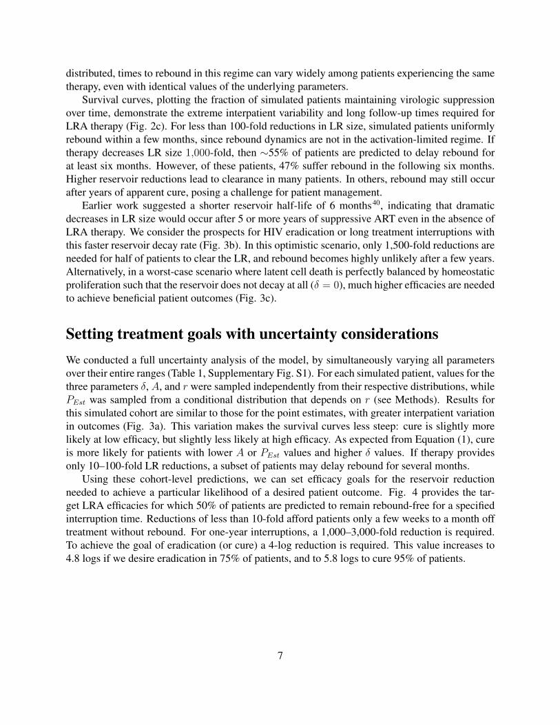
distributed, times to rebound in this regime can vary widely among patients experiencing the sametherapy, even with identical values of the underlying parameters.

Survival curves, plotting the fraction of simulated patients maintaining virologic suppressionover time, demonstrate the extreme interpatient variability and long follow-up times required forLRA therapy (Fig. 2c). For less than 100-fold reductions in LR size, simulated patients uniformlyrebound within a few months, since rebound dynamics are not in the activation-limited regime. Iftherapy decreases LR size 1,000-fold, then ∼55% of patients are predicted to delay rebound forat least six months. However, of these patients, 47% suffer rebound in the following six months.Higher reservoir reductions lead to clearance in many patients. In others, rebound may still occurafter years of apparent cure, posing a challenge for patient management.

Earlier work suggested a shorter reservoir half-life of 6 months40, indicating that dramaticdecreases in LR size would occur after 5 or more years of suppressive ART even in the absence ofLRA therapy. We consider the prospects for HIV eradication or long treatment interruptions withthis faster reservoir decay rate (Fig. 3b). In this optimistic scenario, only 1,500-fold reductions areneeded for half of patients to clear the LR, and rebound becomes highly unlikely after a few years.Alternatively, in a worst-case scenario where latent cell death is perfectly balanced by homeostaticproliferation such that the reservoir does not decay at all (δ = 0), much higher efficacies are neededto achieve beneficial patient outcomes (Fig. 3c).

Setting treatment goals with uncertainty considerationsWe conducted a full uncertainty analysis of the model, by simultaneously varying all parametersover their entire ranges (Table 1, Supplementary Fig. S1). For each simulated patient, values for thethree parameters δ, A, and r were sampled independently from their respective distributions, whilePEst was sampled from a conditional distribution that depends on r (see Methods). Results forthis simulated cohort are similar to those for the point estimates, with greater interpatient variationin outcomes (Fig. 3a). This variation makes the survival curves less steep: cure is slightly morelikely at low efficacy, but slightly less likely at high efficacy. As expected from Equation (1), cureis more likely for patients with lower A or PEst values and higher δ values. If therapy providesonly 10–100-fold LR reductions, a subset of patients may delay rebound for several months.

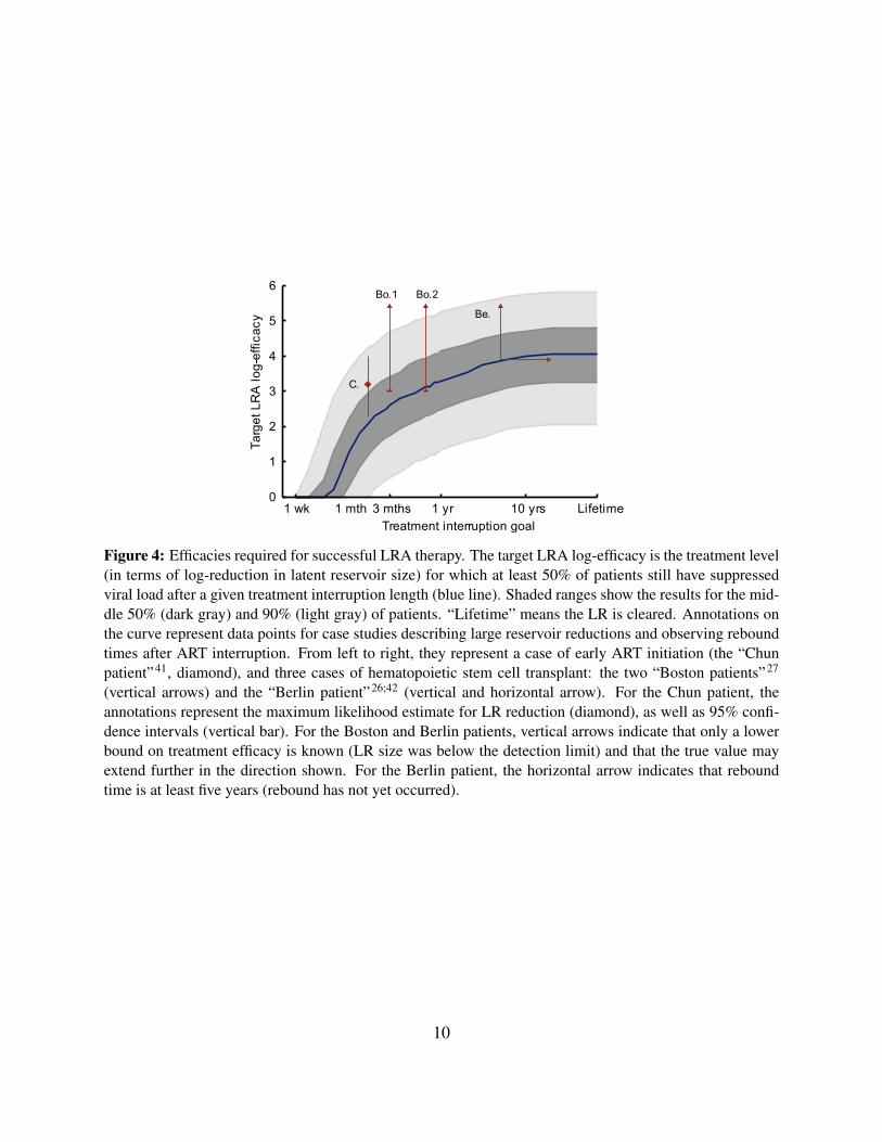
Using these cohort-level predictions, we can set efficacy goals for the reservoir reductionneeded to achieve a particular likelihood of a desired patient outcome. Fig. 4 provides the tar-get LRA efficacies for which 50% of patients are predicted to remain rebound-free for a specifiedinterruption time. Reductions of less than 10-fold afford patients only a few weeks to a month offtreatment without rebound. For one-year interruptions, a 1,000–3,000-fold reduction is required.To achieve the goal of eradication (or cure) a 4-log reduction is required. This value increases to4.8 logs if we desire eradication in 75% of patients, and to 5.8 logs to cure 95% of patients.

7

aI II III

0123456

LRA log-efficacy

0

20

40

60

80

100

% p

atie

nts

supp

ress

ed



LRA log-efficacy

Reb

ound

tim

e (d

ays)

0 1 2 3 4 5 6101

102

103

104

105

0 1 2 3 4 5 6

Pro

b. c

lear

ance

00.20.40.60.8

1

LRA log-efficacy

b

0

20

40

60

80

100

% p

atie

nts

supp

ress

ed



LRA log-efficacy

Reb

ound

tim

e (d

ays)

0 1 2 3 4 5 6101

102

103

104

105

0 1 2 3 4 5 6

Pro

b. c

lear

ance

00.20.40.60.8

1

LRA log-efficacy

c

0

20

40

60

80

100

% p

atie

nts

supp

ress

ed



LRA log-efficacy

Reb

ound

tim

e (d

ays)

0 1 2 3 4 5 610

102

103

104

105

0 1 2 3 4 5 6

Pro

b. c

lear

ance

00.20.40.60.8

1

LRA log-efficacy

Best-case scenario:fast LR decay

Worst-case scenario:no net LR decay

Estimated: average LR half-life 44 months

Figure 3: Predicted LRA therapy outcomes, accounting for uncertainty in patient parameter values. a) Fulluncertainty analysis where all viral dynamics parameters are sampled for each patient from the distributionsprovided in Table 1. b) A best-case scenario where the reservoir half-life is only 6 months (δ = 3.8×10−3).All patients have the same underlying viral dynamic parameters, otherwise given by the point estimates inTable 1. c) A worst-case scenario where the reservoir does not decay because cell death is balanced byhomeostatic proliferation (δ = 0). I) Probability that the LR is cleared by LRA. Clearance occurs if allcells in the LR die before a reactivating lineage leads to viral rebound. “LRA log-efficacy” is the number oforders of magnitude by which the latent reservoir size is reduced following LRA therapy (− log10(q)). II)Median viral rebound times (logarithmic scale), among patients who do not clear the infection. III) Survivalcurves (Kaplan-Meier plots) show the percentage of patients who have not yet experienced viral rebound,plotted as a function of the time (logarithmic scale) after treatment interruption. All simulations included104 to 105 patients.

8

Model applications and comparison to dataCurrent ability to test the model against clinical data is limited both by the dynamic range of assaysmeasuring LR size and by the low efficacy of investigational LRA treatments. Yet we can compareour predictions to results observed for non-LRA-based interventions that lead to decreases in LRsize and prolonged treatment interruptions (Fig. 4). A 2010 study of early ART initiators whoeventually underwent treatment interruption found a single patient with LR size approximately1,500-fold lower than a typical patient (0.0064 infectious units per million resting CD4+ T cells,versus an average of 1 per million) in whom rebound was delayed until 50 days off treatment41. Thewell-known ‘Berlin patient’26 has remained off treatment following a stem-cell transplant since2008, and a comprehensive analysis of his viral reservoirs found HIV DNA levels at least 7,500-fold lower than typical patients in the most sensitive assay42. The two recently reported ‘Bostonpatients’ also interrupted treatment, following transplants that resulted in “at least a 3 to 4 log10decrease” in viral reservoirs27; they have since both rebounded, at approximately 3 and 8 monthspost-interruption. These few available cases demonstrate that our model is not inconsistent withcurrent knowledge. When survival curves for larger cohorts become available, Bayesian methodscan be used to update the estimates in Table 1 and reduce uncertainty of future predictions.

DiscussionOur model is the first to quantify the required efficacy of latency-reversing agents for HIV-1 andset goals for therapy. For a wide range of parameters, we find that therapies must reduce the LR byat least two orders of magnitude to produce a meaningful increase in the time to rebound after ARTinterruption (upward inflection in Figs. 2b, 3II), and that reductions of approximately four ordersof magnitude are needed for half of patients to clear the infection (Figs. 3a, 4). Standard deviationsin rebound times of many months are expected, owing to variation in pretreatment reservoir sizeand exponentially-distributed reactivation times after effective LRA therapy brings the infection toan activation-limited regime. While the efficacy required for these beneficial outcomes is likelybeyond the reach of current drugs, our results permit some optimism: we show for the first timethat reactivation of all cells in the reservoir is not necessary for cessation of ART. This is becausesome cells in the LR will die before reactivating or, following activation, will fail to produce achain of infection events leading to rebound. On a more cautionary note, the wide distributionin reactivation times necessitates careful monitoring of patients, as rebound is possible even afterlong periods of viral suppression.

Even without any reservoir reduction, variation in infection parameters and stochastic acti-vation together predict delays in rebound of at least two months in a small minority of patients(Fig. 4), consistent with ART interruption trials such as SPARTAC43. More detailed (and pos-sibly more speculative) models including specific immune responses may be needed to explainmulti-year post-treatment control, such as found in the VISCONTI cohort28.

Our analysis characterizing the required efficacy of LRA therapy does not rely on the specificmechanism of action of these drugs, only the amount by which they reduce the reservoir. We haveassumed that, after ART/LRA therapy ends, cell activation and death rates return to baseline. We

9

1 wk 1 mth 3 mths 1 yr 10 yrs Lifetime0

1

2

3

4

5

6

Treatment interruption goal

Targ

et L

RA

log-

effic

acy

C.

Bo.1 Bo.2

Be.

Figure 4: Efficacies required for successful LRA therapy. The target LRA log-efficacy is the treatment level(in terms of log-reduction in latent reservoir size) for which at least 50% of patients still have suppressedviral load after a given treatment interruption length (blue line). Shaded ranges show the results for the mid-dle 50% (dark gray) and 90% (light gray) of patients. “Lifetime” means the LR is cleared. Annotations onthe curve represent data points for case studies describing large reservoir reductions and observing reboundtimes after ART interruption. From left to right, they represent a case of early ART initiation (the “Chunpatient”41, diamond), and three cases of hematopoietic stem cell transplant: the two “Boston patients”27

(vertical arrows) and the “Berlin patient”26;42 (vertical and horizontal arrow). For the Chun patient, theannotations represent the maximum likelihood estimate for LR reduction (diamond), as well as 95% confi-dence intervals (vertical bar). For the Boston and Berlin patients, vertical arrows indicate that only a lowerbound on treatment efficacy is known (LR size was below the detection limit) and that the true value mayextend further in the direction shown. For the Berlin patient, the horizontal arrow indicates that reboundtime is at least five years (rebound has not yet occurred).

10

have also assumed that the reservoir is a homogeneous population without variation in activationand death rates. The presence of reservoir compartments with different levels of drug penetrationdoes not alter our results, as they are stated in terms of total reservoir reduction. If, however, thesecompartments vary in activation or death rates44, or if viral dynamics of activated cells dependson their source compartment, then our model may need to be modified. In the absence of clearunderstanding of multiple compartments constituting the LR, we have considered the simplestscenario which may be able to fit future LRA therapy outcomes.

Our model also highlights the importance of measuring specific parameters describing latencyand infection dynamics. Despite the field’s focus on measuring latent reservoir size with increasingaccuracy45;46, our results suggest that the rate at which latently infected cells activate — and thefraction of these that are expected to establish a rebounding infection — are more predictive ofLRA outcomes. Among all parameters that determine outcome, the establishment probability isleast understood, as it cannot be measured from viral load dynamics above the limit of detection.Simply because an integrated provirus is replication-competent and transcriptionally active doesnot mean that it will initiate a growing infection: as with all population dynamics, chance eventsdominate early stages of infection growth39;47. Full-length HIV-1 transcription is itself a stochasticprocess, governed by fluctuating concentrations of early gene products48. Sensitive assays of viraloutgrowth may pave the way toward understanding the importance of these chance events to earlyinfection; for example, ongoing experiments using fluorescent imaging of in vitro infections seededby single cells productively infected with a reporter HIV strain suggest that only 14% trigger agrowing infection before their lineage dies out (G. Laird, personal communication). The stochasticnature of HIV-1 infection dynamics implies that even similarly situated patients may experiencedivergent responses to LRA therapy.

The model can also advise aspects of trial design for LRAs. Survival curves computed fromequation (S9) can be used to predict the probability that a patient is cured, given that they havebeen off treatment without rebound for a known period. As frequent viral load testing for yearsof post-interruption monitoring is not feasible, it may be helpful to choose sampling timepointsbased on the expected distribution of rebound times. Trial design is complicated by the fact thatLRA treatment efficacy is unknown if post-treatment LR size is below the detection limit. Byconsidering prior knowledge about viral dynamics parameters and the range of possible treatmentefficacies, the model can be used to estimate outcomes even in the presence of uncertainty.

To date, laboratory and clinical studies of investigational LRAs have generally found weakpotential for reservoir reduction — up to one log-reduction in vitro and less in vivo16;30;49. Wepredict that much higher efficacy will be required for eradication, which may be achieved by mul-tiple rounds of LRA therapy, a combination of therapies, or development of therapies to which agreater fraction of the LR is susceptible. While we have focused on LRA therapy, our findingsalso serve to interpret infection eradication or delays in rebound caused by early treatment28;29;50;51

or stem cell transplantation26;27, both of which also reduce the latent reservoir. We believe thatthese modeling efforts will provide a quantitative framework for interpreting clinical trials of anyreservoir-reduction strategy.

11

AcknowledgementsWe thank Ya-chi Ho, S. Alireza Rabi, Liang Shan, and Greg Laird for insightful discussions and forsharing data. This work was supported by the Martin Delaney CARE and DARE Collaboratories(NIH grants AI096113 and 1U19AI096109), by an ARCHE Collaborative Research Grant fromthe Foundation for AIDS Research (amFAR 108165-50-RGRL), by the Johns Hopkins Center forAIDS Research, by NIH grant 43222, and by the Howard Hughes Medical Institute. MAN wassupported by the John Templeton Foundation. FF was funded by a European Research CouncilAdvanced Grant (PBDR 268540). ALH and DISR were supported by a Bill & Melinda GatesFoundation Grand Challenges Explorations Grant (OPP1044503).

References[1] Chun, T. W., et al. Quantification of latent tissue reservoirs and total body viral load in HIV-1

infection. Nature 387(6629), 183–188 (1997).

[2] Chun, T. W., et al. Early establishment of a pool of latently infected, resting CD4(+) T cellsduring primary HIV-1 infection. Proc. Natl. Acad. Sci. USA 95(15), 8869–8873 (1998).

[3] Finzi, D., et al. Identification of a reservoir for HIV-1 in patients on highly active antiretro-viral therapy. Science 278(5341), 1295–1300 (1997).

[4] Wong, J. K., et al. Recovery of replication-competent HIV despite prolonged suppression ofplasma viremia. Science 278(5341), 1291–1295 (1997).

[5] Chun, T. W., et al. Presence of an inducible HIV-1 latent reservoir during highly activeantiretroviral therapy. Proc. Natl. Acad. Sci. USA 94(24), 13193–13197 (1997).

[6] Siliciano, J. D., et al. Long-term follow-up studies confirm the stability of the latent reservoirfor HIV-1 in resting CD4+ T cells. Nat. Med. 9(6), 727–728 (2003).

[7] Archin, N. M., et al. Measuring HIV latency over time: Reservoir stability and assessinginterventions. In 21st Conference on Retroviruses and Opportunistic Infections, Boston, MA,(2014).

[8] Ruiz, L., et al. Structured treatment interruption in chronically HIV-1 infected patients afterlong-term viral suppression. AIDS 14(4), 397 (2000).

[9] Davey, Jr., R. T., et al. HIV-1 and T cell dynamics after interruption of highly active antiretro-viral therapy (HAART) in patients with a history of sustained viral suppression. Proc. Natl.Acad. Sci. USA 96(26), 15109–15114 (1999).

[10] Marsden, M. D. & Zack, J. A. Establishment and maintenance of HIV latency: model systemsand opportunities for intervention. Future Virol 5(1), 97–109 (2010).

12

[11] Hakre, S., Chavez, L., Shirakawa, K., & Verdin, E. Epigenetic regulation of HIV latency.Curr. Opin. HIV AIDS 6(1), 19–24 (2011).

[12] Mbonye, U. & Karn, J. Control of HIV latency by epigenetic and non-epigenetic mechanisms.Curr HIV Res. 9(8), 554–567 (2011).

[13] Ruelas, D. S. & Greene, W. C. An integrated overview of HIV-1 latency. Cell 155(3), 519–529 (2013).

[14] Choudhary, S. K. & Margolis, D. M. Curing HIV: pharmacologic approaches to target HIV-1latency. Ann. Rev. Pharmacol. Toxicol. 51(1), 397–418 (2011).

[15] Durand, C. M., Blankson, J. N., & Siliciano, R. F. Developing strategies for HIV-1 eradica-tion. Trends Immunol 33(11), 554–562 (2012).

[16] Archin, N. M., et al. Antiretroviral intensification and valproic acid lack sustained effect onresidual HIV-1 viremia or resting CD4+ cell infection. PLoS ONE 5(2), e9390 (2010).

[17] Archin, N. M., et al. Administration of vorinostat disrupts HIV-1 latency in patients onantiretroviral therapy. Nature 487(7408), 482–485 (2012).

[18] Shirakawa, K., Chavez, L., Hakre, S., Calvanese, V., & Verdin, E. Reactivation of latent HIVby histone deacetylase inhibitors. Trends Microbiol 21(6), 277–285 (2013).

[19] Korin, Y. D., Brooks, D. G., Brown, S., Korotzer, A., & Zack, J. A. Effects of prostratinon T-cell activation and human immunodeficiency virus latency. J Virol 76(16), 8118–8123(2002).

[20] Williams, S. A., et al. Prostratin antagonizes HIV latency by activating NF-kappaB. J. BiolChem 279(40), 42008–42017 (2004).

[21] Mehla, R., et al. Bryostatin modulates latent HIV-1 infection via PKC and AMPK signalingbut inhibits acute infection in a receptor independent manner. PloS ONE 5(6), e11160 (2010).

[22] DeChristopher, B. A., et al. Designed, synthetically accessible bryostatin analogues potentlyinduce activation of latent HIV reservoirs in vitro. Nat Chem 4(9), 705–710 (2012).

[23] Bartholomeeusen, K., Xiang, Y., Fujinaga, K., & Peterlin, B. M. Bromodomain and extra-terminal (BET) bromodomain inhibition activate transcription via transient release of positivetranscription elongation factor b (p-TEFb) from 7SK small nuclear ribonucleoprotein. J. BiolChem 287(43), 36609–36616 (2012).

[24] Zhu, J., et al. Reactivation of latent HIV-1 by inhibition of BRD4. Cell Rep. 2(4), 807–816(2012).

[25] Boehm, D., et al. BET bromodomain-targeting compounds reactivate HIV from latency viaa tat-independent mechanism. Cell Cycle 12(3), 452–462 (2013).

13

[26] Hutter, G., et al. Long-term control of HIV by CCR5 Delta32/Delta32 stem-cell transplanta-tion. New Engl J Med 360(7), 692–698 (2009). PMID: 19213682.

[27] Henrich, T. J., et al. HIV-1 rebound following allogeneic stem cell transplantation and treat-ment interruption. In 21st Conference on Retroviruses and Opportunistic Infections, Boston,MA, (2014).

[28] Saez-Cirion, A., et al. Post-treatment HIV-1 controllers with a long-term virological remis-sion after the interruption of early initiated antiretroviral therapy ANRS VISCONTI study.PLoS Pathog 9(3), e1003211 (2013). PMID: 23516360.

[29] Persaud, D., et al. Absence of detectable HIV-1 viremia after treatment cessation in an infant.New Engl J Med 369(19), 1828–1835 (2013). PMID: 24152233.

[30] Cillo, A. Only a small fraction of HIV-1 proviruses in resting CD4+ T cells can be inducedto produce virions ex vivo with anti-CD3/CD28 or vorinostat. In 20th Conference on Retro-viruses and Opportunistic Infections, Atlanta, GA, (2013).

[31] Bullen, C. K., Laird, G. M., Durand, C. M., Siliciano, J. D., & Siliciano, R. F. New ex vivoapproaches distinguish effective and ineffective single agents for reversing HIV-1 latency invivo. Nat. Med. in press.

[32] Spivak, A. M., et al. A pilot study assessing the safety and latency-reversing activity ofdisulfiram in HIV-1Infected adults on antiretroviral therapy. Clin Infect Dis 58(6), 883–890(2014). PMID: 24336828.

[33] Perelson, A. S., et al. Decay characteristics of HIV-1-infected compartments during combi-nation therapy. Nature 387(6629), 188–191 (1997).

[34] Nowak, M. A. & May, R. M. C. Virus Dynamics: Mathematical principles of immunologyand virology. Oxford Univ. Press, USA, (2000).

[35] Archin, N. M., et al. Immediate antiviral therapy appears to restrict resting CD4+ cell HIV-1 infection without accelerating the decay of latent infection. Proc. Natl. Acad. Sci. USA109(24), 9523–9528 (2012).

[36] Sedaghat, A. R., Siliciano, J. D., Brennan, T. P., Wilke, C. O., & Siliciano, R. F. Limits onreplenishment of the resting CD4+ T cell reservoir for HIV in patients on HAART. PLoSPathog 3(8), e122 (2007).

[37] Conway, J. M. & Coombs, D. A stochastic model of latently infected cell reactivation andviral blip generation in treated HIV patients. PLoS Comput Biol 7(4), e1002033 (2011).

[38] Rosenbloom, D. I. S., Hill, A. L., Rabi, S. A., Siliciano, R. F., & Nowak, M. A. Antiretroviraldynamics determines HIV evolution and predicts therapy outcome. Nat. Med. 18(9), 1378–1385 (2012).

14

[39] Pearson, J. E., Krapivsky, P., & Perelson, A. S. Stochastic theory of early viral infection:Continuous versus burst production of virions. PLoS Comput Biol 7(2), e1001058 (2011).

[40] Zhang, L., et al. Quantifying residual HIV-1 replication in patients receiving combinationantiretroviral therapy. New Engl J Med 340(21), 1605–1613 (1999). PMID: 10341272.

[41] Chun, T.-W., et al. Rebound of plasma viremia following cessation of antiretroviral therapydespite profoundly low levels of HIV reservoir: implications for eradication. AIDS 24(18),2803–2808 (2010). PMID: 20962613 PMCID: PMC3154092.

[42] Yukl, S. A., et al. Challenges in detecting HIV persistence during potentially curative inter-ventions: A study of the Berlin Patient. PLoS Pathog 9(5), e1003347 (2013).

[43] Stohr, W., et al. Duration of HIV-1 viral suppression on cessation of antiretroviral therapy inprimary infection correlates with time on therapy. PloS one 8(10), e78287 (2013).

[44] Buzon, M. J., et al. HIV-1 persistence in CD4(+) T cells with stem cell-like properties. NatMed 20(2), 139–142 (2014).

[45] Laird, G. M., et al. Rapid quantification of the latent reservoir for HIV-1 using a viral out-growth assay. PLoS Pathog 9(5), e1003398 (2013). PMID: 23737751 PMCID: PMC3667757.

[46] Ho, Y.-C., et al. Replication-competent noninduced proviruses in the latent reservoir increasebarrier to HIV-1 cure. Cell 155(3), 540–551 (2013). PMID: 24243014.

[47] Hofacre, A., Wodarz, D., Komarova, N. L., & Fan, H. Early infection and spread of a condi-tionally replicating adenovirus under conditions of plaque formation. Virology 423(1), 89–96(2012). PMID: 22192628.

[48] Singh, A. & Weinberger, L. S. Stochastic gene expression as a molecular switch for virallatency. Curr Opin in Microbiol 12(4), 460–466 (2009).

[49] Xing, S., et al. Disulfiram reactivates latent HIV-1 in a bcl-2-transduced primary CD4+ Tcell model without inducing global T cell activation. J. Virol. 85(12), 6060–6064 (2011).

[50] Blankson, J. N., Siliciano, J. D., & Siliciano, R. F. The Effect of early treatment on the latentreservoir of HIV-1. J. Infect. Dis. 191(9), 1394–1396 (2005).

[51] Strain, M. C., et al. Effect of treatment, during primary infection, on establishment andclearance of cellular reservoirs of HIV-1. J. Infect. Dis. 191(9), 1410–1418 (2005).

[52] Luo, R., Piovoso, M. J., Martinez-Picado, J., & Zurakowski, R. HIV model parameter esti-mates from interruption trial data including drug efficacy and reservoir dynamics. PLoS ONE7(7), e40198 (2012).

[53] Rouzine, I. M. & Coffin, J. M. Linkage disequilibrium test implies a large effective populationnumber for HIV in vivo. Proc. Natl. Acad. Sci. USA 96(19), 10758–10763 (1999).

15

[54] Pennings, P. S. Standing genetic variation and the evolution of drug resistance in HIV. PLoSComput Biol 8(6), e1002527 (2012).

[55] Pennings, P. S., Kryazhimskiy, S., & Wakeley, J. Loss and recovery of genetic diversity inadapting populations of HIV. PLoS Genetics 10(1), e1004000 (2014).

[56] Eriksson, S., et al. Comparative analysis of measures of viral reservoirs in HIV-1 eradicationstudies. PLoS Pathog 9(2), e1003174 (2013).

[57] Karlin, S. & Taylor, H. E. A First Course in Stochastic Processes. Academic Press, SanDiego, (1975).

[58] De Boer, R. J., Ribeiro, R. M., & Perelson, A. S. Current estimates for HIV-1 productionimply rapid viral clearance in lymphoid tissues. PLoS Comput Biol 6(9), e1000906 (2010).

[59] Di Mascio, M., et al. Noninvasive in vivo imaging of CD4 cells in simian-human immunod-eficiency virus (SHIV)-infected nonhuman primates. Blood 114(2), 328–337 (2009).

[60] Ganusov, V. V. & De Boer, R. J. Do most lymphocytes in humans really reside in the gut?Trends Immunol 28(12), 514–518 (2007).

[61] Chen, H. Y., Di Mascio, M., Perelson, A. S., Ho, D. D., & Zhang, L. Determination of virusburst size in vivo using a single-cycle SIV in rhesus macaques. Proc. Natl. Acad. Sci. USA104(48), 19079–19084 (2007).

[62] Reilly, C., Wietgrefe, S., Sedgewick, G., & Haase, A. Determination of simian immunodefi-ciency virus production by infected activated and resting cells. AIDS 21(2), 163–168 (2007).

[63] Markowitz, M., et al. A novel antiviral intervention results in more accurate assessment ofhuman immunodeficiency virus type 1 replication dynamics and T-cell decay in vivo. J. Virol.77(8), 5037–5038 (2003).

[64] Ribeiro, R. M., et al. Estimation of the initial viral growth rate and basic reproductive numberduring acute HIV-1 infection. Journal of Virology 84(12), 6096 –6102 (2010).

[65] Sigal, A., et al. Cell-to-cell spread of HIV permits ongoing replication despite antiretroviraltherapy. Nature 477(7362), 95–98 (2011).

[66] Kouyos, R. D., Althaus, C. L., & Bonhoeffer, S. Stochastic or deterministic: what is theeffective population size of HIV-1? Trends Microbiol 14(12), 507–511 (2006).

[67] Abate, J., Choudhury, G. L., & Whitt, W. An introduction to numerical transform inversionand its application to probability models. In Computational Probability, Grassmann, W. K.,editor, number 24 in International Series in Operations Research & Management Science,257–323. Springer US (2000).

16

Methods

Stochastic model of viral dynamicsThe basic model of reservoir dynamics and rebound tracks two cell types: productively infectedactivated CD4+ T cells, and latently infected resting CD4+ T cells. Cells with nonviable provirus,which may vastly outnumber those with replication-competent provirus56, are excluded. Themodel can be described formally as a two-type branching process, in which four types of eventscan occur (Fig. 1):

Z → Y ... rate constant: aZ → ∅... rate constant: dzY → cY ... rate constant: b× pλ(c)Y → ∅... rate constant: d

(2)

In this notation Y and Z represent individual actively or latently infected cells, respectively,∅ represents no cells, and the arrows represent events that lead one type of cell to become theother type. A latently infected cell can either activate (at rate a) or die (at rate dz). An activelyinfected cell can either die (at rate d) or produce a burst of virions (at rate b) that results in theinfection of c other cells, where c is a Poisson-distributed random variable with parameter λ,pλ(c) = (exp(−λ)λc) /(c!). After a burst event, the original cell dies. This model is similar toother stochastic models of viral dynamics39.

Each infection is independent and occurs within a large, constant target cell population. Asthe model does not include limitations on viral growth, it describes only the initial stages of viralrebound. Since clinical rebound thresholds (plasma HIV RNA > 50 – 200 c ml−1) are well belowtypical setpoints (104 – 106 c ml−1), this model suffices to analyze rebound following LRA therapyand ART interruption. We do not explicitly track free virus, but assume it is at a level propor-tional to the number of infected cells. This assumption is valid because the rates governing theproduction of virus from infected cells and the clearance rate of free virus are much higher thanother rates, allowing a separation of time scales. Because we are not interested in blips or otherintraday viral dynamics, this assumption does not influence our results. A method for calculatingthe proportionality between free virus and infected cells is provided below.

The growth rate of the infection is r = b(λ − 1) − d. The total death rate of infected cells isdy = b + d, and the basic reproductive ratio (mean offspring number for a single infected cell) isR0 =

bλb+d

. The establishment probability PEst is the solution to R0

(1− e−λPEst

)− λPEst = 0.

Generating function analysis of modelA simplified version of the above branching process was used, for which probability generatingfunctions could be written and expanded explicitly. In this simplified process, each birth event re-sults in exactly two actively infected cells. The initial number of latently infected cells was treatedas Poisson-distributed around expected value qNLR, where NLR is the pre-therapy LR size and q

17

represents therapy efficacy. The initial number of actively infected cells was treated as Poisson-distributed around aqNLR/(b+d), representing activation-death equilibrium during effective treat-ment (birth events failing to produce new infected cells) with latently infected cells held constantat qNLR. Latent cell dynamics following interruption were the same as in the model describedabove. The backwards Kolmogorov equations for this process57 can be solved explicitly, resultingin a probability generating function for the number of actively infected cells existing at time t. Inthe Supplementary Methods, we derive the clearance probability PClr ≈ exp [−qAPEst/δ] and theprobability that there are Y actively infected cells at time t:

P (Y , t) ≈ exp

−qAPEstω1 +

1− eδt(1 + δ

∫ t0g(τ)dτ

)δPEst

× 1

Y !

(ert − 1

ert − 1 + PEst

)Y× (ω2)Y M

(−Y , ω2,−

qAP 2Est

2− PEstω1

),

(3)

where ω1 = (ertPEst) / (r (ert − 1) (ert − 1 + PEst)), ω2 =

(qAPEste

−δt) /r, g(t) =eδt (ert − 1) (1− PEst) / (ert − 1 + PEst), ()Y is the Pochhammer symbol (rising factorial), andM is Kummer’s confluent hypergeometric function. Both approximations hold for δ much smallerthan r. In the Supplementary Methods, we also provide an efficient method for calculating re-bound probabilities without repeated evaluation of Eq. (3) at multiple values of Y . This efficientmethod allows for computation of all survival curves in Fig. 2 in seconds. A script is providedat http://www.danielrosenbloom.com/reboundtimes to rapidly compute survivalcurves using these methods.

Estimating the cell-to-virus ratioBecause the model tracks only infected cells, but must relate total body cell counts to clinically ob-served plasma viral RNA concentrations, we require an estimate of the conversion factor betweenthese two quantities. For this calculation we applied a version of the analysis developed in De Boeret al.58. Let Y be the total body number of productively infected cells residing in lymphoid tissue,let V be the total body number of free virus particles, and let κ be the per-cell production rate ofvirions. We can balance viral production and decay at equilibrium for a typical 70-kg indivivdual:

κY = dvV

=

(dvκ

)(100 virions in LT1 virion in ECF

)(1 virion in ECF

2 RNA copies in ECF

)(15,000 ml ECF) v

=

(dvκ

)(7.5× 105

virions in LTRNA copies per ml ECF

)v,

(4)

where v is the per-ml concentration of viral RNA in circulation. Here we use the estimate thatvirus particles in the lymphoid tissue outnumber those in circulation 100-fold, mirroring the ratio

18

http://www.danielrosenbloom.com/reboundtimes

of lymphocytes in lymph nodes versus in circulation59;60. Note that since the lifespan of an infectedcell is much longer than that of a free virion, the ratio of production to decay rates, κ/dv, equals thenumber of free virions associated with a productive cell during most of that cell’s existence; valuesof 200–1000 are consistent with recent experiments58;61;62. The resulting estimate forY is therefore(750 to 3750)× v. We use the geometric mean of these values – 1680 – as a point estimate. Withthis value the viral rebound threshold of 200 c ml−1corresponds to Y ≈ 3× 105. Note that modelresults are insensitive to this value, as rebound probability depends on the logarithm of the reboundthreshold.

Estimating key parametersEstimation of δ

The net decay rate of the latent reservoir (δ) was estimated from a previous study of longitudinalreservoir size in patients on long-term ART. Table 1 of Siliciano et al.6 reports the mean and 95%confidence interval of LR decay from a cohort of 59 patients, derived using a mixed-effects model.This method models each patient’s decay rate δi as being sampled from a population-level normaldistribution with mean 5.2×10−4 d−1 and standard deviation of 1.6×10−4. We use this distributionto sample simulated patients. Note that with this method, approximately 1 in 1500 draws will givea negative value of δ, corresponding to an LR that fails to decay (e.g., by homeostatic proliferationoutweighting activation plus death). We allowed negative δ only for simulation of the model withhomeostatic proliferation; for all others, we truncated the distribution at zero.

The mean decay rate from the Siliciano study corresponds to a reservoir half-life of 44 months,which is consistent with a more recent study that found a value of 43 months7.

Estimation of r

The net exponential growth rate of the infection (r) and the number of latent cells reactivating perday (A) before reservoir-reducing therapy can be estimated from ART-interruption studies. Luoet al.52 report the joint posterior distributions of viral dynamic parameters for 10 patients whounderwent 3-5 structured treatment interruptions in a previous study8. From these, we computedinter-patient distributions for both r and A.

The authors used a system of three differential equations to describe viral rebound duringtreatment interruption: x(t) = λx − dxx(t) − βx(t)v(t), y(t) = βx(t)v(t) − dyy(t) + λy, andv(t) = γy(t) − dvv(t); where state variables x, y, and v represented plasma concentrations ofuninfected CD4+ T cells, productively infected CD4+ T cells, and free virus, respectively. Param-eters λx and dx denote production and death rates of target cells, respectively; β is infectivity; dyis the total death rate of infected cells; γ is the viral production rate by infected cells; dv is theviral clearance rate; and λy represents the rate at which latently infected cells activate to becomeproductively infected cells.

The desired parameter r is the net growth rate of the infection at low viral loads, and in terms ofthe paper’s model, corresponds to: r = (βλγ)/(dxdv)− dy. To estimate the population-level pos-terior distribution for r, we used the paper’s reported posterior distributions of the basic parameters

19

for each patient. They reported these distributions as a list of 200,000 samples for each patient,from which we ignored the first 50,000 to allow convergence and used the remaining 150,000 asthe individual-level posterior estimate for that patient. We then treated each posterior estimate oflog(r) as a random normal variable sampled from N (µi, σi), where each patient’s µi is sampledfrom N (µ, σ). Population parameters were estimated by maximum likelihood using the mvmetalibrary in R to be µ = −0.398 and σ = 0.194. The geometric mean of the corresponding lognormaldistribution therefore corresponds to r = 0.4 d−1.

We confirmed these values with data from a separate treatment interruption trial9, using a least-squares fit to exponential growth of viral load shortly after rebound. This analysis again produceda geometric mean value of r = 0.4 d−1.

Another commonly used measure of viral fitness is the basic reproductive ratio R0, whichdescribes the average number of new cells infected by virus from a single actively infected cell. Thegrowth rate and the basic reproductive ratio relate to each other asR0 = r/dy+1, where dy = b+d.Using the well-established average lifespan of infected CD4+ T cells of 1 day (measured fromviral load decay during ART63) a growth rate of r = 0.4 corresponds to R0 = 1.4. This basicreproductive ratio observed during ART interruption is consistently lower than that observed duringacute infection (for which R0 ≈ 8− 10)38;64, likely due to improved immune response.

Estimation of A

We use the Luo et al.52 data and a similar procedure to estimate A, the number of cells exiting theLR per day during fully suppressive ART, which is proportional to the initial residual viral loadfrom which rebound begins. As this data included densely sampled viral load, but few measure-ments of CD4+ T cells, the fitted parameters are most reliable in determining virological quantities,not cell counts. For example, the quantity (γλy)/(dvdy), which equals the residual viral load ob-served during fully suppressive therapy, should be particularly reliable. Additionally, dy itself canbe reliably determined the decay of viral load upon resumption of therapy63. Since it is the productof two reliable parameters, the rate of virus production during ART (λv = (γλy)/dv) will also be areliable quantity to estimate. In contrast, the cellular rate λy by itself may not be reliably estimatedfrom this data. In fact, since Luo et al.52 identified the sum x(t) + y(t) with total CD4 count,though the majority of CD4+ T cells are not actually infectable, they should systematically reportan overestimate of parameter λy. We therefore felt that A could be estimated more robustly byexploiting its proportionality to reliably estimated viral rates.

We estimate A in two steps: (1) use the posterior distributions reported by Luo et al.52 toestimate the interpatient distribution for λv, which has units of copies of viral RNA per ml plasma,per day; (2) use separate observations regarding the ratio of cells to virus to scale λv to A, whichhas units of (total body) infected CD4+ T cells per day. Analogously to the above estimationof r, we estimated a lognormal interpatient distribution for λv, obtaining log mean and standarddeviation −1.469 and 0.991, respectively. To scale to A, we used the cell-to-virus ratio describedabove, which implies that A is (750 to 3750) × λv. To obtain a normal distribution for log(A),we treated the extremes of 750 and 3750 as estimates of the 95% CI for the ratio A/λv, adding12(log(750) + log(3750)) = 3.225 to the mean and 0.178 to the standard deviation. The resulting

distribution for A has log mean and standard deviation 1.755 and 1.007, respectively.

20

Estimation of PEst

Measuring establishment probabilities in early stages of infections is a difficult task that requiresfrequent tracking of rare infection and extinction events in small populations (e.g., Hofacre et al.47).In contrast, even the most sensitive methods currently used to measure growth of HIV over timein vitro do not yet provide single-cell resolution45;65. In the absence of the relevant experimentalresults, we rely on population genetic models to estimate PEst.

In the basic stochastic model described above, the establishment probability is mainly con-trolled by the parameter λ. For a fixed growth rate r, higher λ values correspond to lower valuesof PEst. To generalize this concept to measures more common in population genetics, we reframePEst in terms of the quantity ρ – the ratio of the variance to the mean offspring number for a singlecell. In our basic model, ρ = 1 + dλ/(b + d), as the mean offspring number (basic reproduc-tive ratio) is R0 = bλ/(b + d) and the variance is

(b(λ+ (λ−R0)

2)+ dR20

)/(b + d). Thus the

establishment probability depends only on ρ and R0 and is the solution to

PEst (R0 + ρ− 1) = R0

(1− e−PEst(R0+ρ−1)

). (5)

Using this equation we can use estimates of ρ from various data sources to derive a range ofreasonable values for PEst.

The maximum establishment probability compatible with a fixed viral fitness R0 occurs whend = 0, which sets ρ = 1 and results in PEst being determined by the equation PEst = 1−e−PEstR0 .This equation corresponds to the establishment probability relationship derived by Pennings54 andby Pearson et al.39 for their “burst model.” Thus the ρ = 1 limit sets a natural upper bound forPEst.

To estimate a lower bound for PEst, note that the ratio ρ measures the deviation of viral repli-cation from a simple Poisson process. Population genetic studies have consistently measured theeffective population size (Ne) of an individual host’s infection as far smaller than the total numberof cells infected with HIV (N )66, an indication of greater-than-Poisson variance in the replicationprocess. The ratio N/Ne reports an order-of-magnitude estimate for ρ. Since equilibrium modelsof neutral diversity may not be applicable to a population such as HIV that undergoes frequentselective sweeps55;66, we consider two studies based on models of selective sweeps, both of whichconverge upon an estimate of Ne ≈ 105 for patients on either no treatment or ineffective treat-ment53;55. Using N ≈ 108 as a typical number of infected cells off therapy, these studies implyρ ≈ 103.

Some care is required to interpret this value in the context of our model: since these studiesexamined diverse, evolving viral populations, strains with low relative fitness tend to contributenegligibly toNe

55. In the small-infection regime of our model, however, relative fitness differencesbetween strains are unimportant, and any virus that is viable (in the sense of absolute fitness, r > 0or R0 > 1) is capable of establishing a rebounding infection. The estimate ρ ≈ 103 is therefore aconservative upper bound for the true value of ρ, providing a lower bound for PEst.

The most relevant estimate for the establishment probability to our knowledge comes froman analysis of the rate of emergence of drug-resistant variants from the latent reservoir duringfully suppressive ART. This study calculated an “effective exit rate” from the latent reservoir of 5productively infected cells per day54. When compared to our estimate of A centered at 57 cells per

21

day (1), this implies ρ ≈ 57/5 = 11.4. We therefore use ρ ≈ 10 as the best parameter estimate andthe center of sampled range.

To capture the current state of knowledge and represent our uncertainty, we use a lognormaldistribution for ρ centered at 10 with 95% of the distribution falling between 1 and 100. Aftersampling r and ρ, we compute R0 (described above in the section on estimating r) and then PEst(using Eq. (5)). Interestingly, a recent experiment measured the in vitro establishment probabilityof a single cell productively infected with a reporter HIV strain to be 14%, which is at the 70thpercentile of our distribution (G. Laird, personal communication).

Analysis of alternate stochastic modelsThe basic five-parameter, two-variable model described above was used to derive the result that theoutcomes of reservoir-reducing therapy depend only on four “key parameters,” which are not nec-essarily model-specific. To test the robustness of this claim to structural variation in model choice,we constructed a series of alternate stochastic models, some of which include more complex infec-tion processes. For each model, we derived expressions relating the model-specific parameters tothe four key parameters. We then simulated the model and compared it to simulations of the basicmodel with identical values of the key parameters. There is generally an infinite set of model-specific parameters satisfying the same key parameter values; where needed, we evaluated a fewexamples at the extremes of what could be considered biologically realistic. A full descriptionof the models, parameters, and results is given in the Supplementary Materials. In summary, thealternate models were:

1. Constant burst model: Infected cells either die without infecting, or produce a fixed (integer)number of new infected cells.

2. Eclipse phase model: Upon reactivation from latency or new infection, cells enter an “eclipsephase” in which they cannot infect others (no virus is produced). Cells in the eclipse phasemay either die or proceed to the productively infected phase, where they behave as infectedcells do in the constant burst model. We consider a eclipse phase of average length 2 dayswith 1/6 chance of death.

3. Free virus model: We explicitly track the amount of free virus. Infected cells either diewithout infecting, or produce a fixed (integer) number of virions. Each virion may eitherbe cleared or may infect a new cell. We consider viral burst sizes ranging from 10 to 1000virions.

4. Homeostatic proliferation: Latently infected cells can either reactivate, die, or divide withoutreactivating giving rise to another latently infected cell. To test a reasonable biologicallimit of fast turnover, cells have an average lifespan of 6 months, but the net LR half-life ismaintained at 44 months by proliferation.

5. Bursting homeostatic proliferation: Latently infected cells can either reactivate, die, or dividemultiple times without reactivating giving rise to a burst of other latently infected cells. To

22

test a biological limit of fast turnover, cells have an average lifespan of 6 months, but the netLR half-life is maintained at 44 months by proliferation with 4 divisions leading to 16 cells.

6. Expansion upon reactivation: When latently infected cells reactivate, they first proliferatemultiple times without infecting others. Thus each reactivated latent cell results in multipleproductively infected cells. We consider a maximum of 4 divisions leading to 16 newlyreactivated cells.

Simulation of the modelWe use the Gillespie algorithm to track the number of latently and actively infected cells ina continuous time stochastic process. We start with an initial number of latent cells Z(0) ∼Binomial(NLR, q), where NLR is the pre-treatment reservoir size and q is the efficacy of LRAtreatment (fraction of cells remaining). The initial number of actively infected cells Y(0) is thenchosen from a Poisson distribution with parameter aZ(0)/dy (corresponding to the immigration-death equilibrium of the branching process). The simulation proceeds until the number of activelyinfected cells reaches the threshold for clinical detection given by a viral load of 200 c ml−1 (equiv-alent to Y = 3× 105 cells total) or until no active or latent cells remain. Because stochastic effectsare important only for small Y , we switch to faster deterministic numerical integration when Yreaches a level where the probability of extinction is very low (< 10−4). For each q value weperform 104 to 105 simulations.

Simulations are seeded with values of the key parameters (δ, A, r, PEst), which may be eitherthe point estimates or random numbers sampled from the distributions in Table 1. We then backout values of the model-specific parameters that are consistent with the sampled key parameters.In general, we use a pre-therapy LR size of NLR = 106 cells to get a = A/NLR. We then havedz = δ−a. Using r and ρ along with dy = d+b = 1 day−1, we can get λ, b, d, and PEst. Consistentwith our generating function analysis, we find that the specific values assumed for NLR and dy donot influence the results. For simulating other models, any other parameter assumptions are listedin the corresponding supplementary figure captions.

23

Supplementary Figures

Freq

uenc

y

Establishment probability, PEst

10−4 10−3 10−2 0.1 10

0.2

0.4

0.6

0.8

1

Freq

uenc

y

Infection growth rate, r ( day-1)0 1 2

0

0.2

0.4

0.6

0.8

1

LR half−life, ln(2) /δ (months)

Freq

uenc

y

0 10 20 30 40 50 60 70 80 90 1000

0.2

0.4

0.6

0.8

1

Baseline LR exit rate, A (cells day-1)

Freq

uenc

y

10−2 1 102 104

0.2

0.4

0.6

0.8

1

0

b

c d

a

Figure S1: Parameter distributions described in Table 1 and used for results in Figs. 3 (uncertainty analysis)and 4 (target LRA efficacy)

24

a b c0123456

LRA log-efficacy

0

20

40

60

80

100

% p

atie

nts

supp

ress

ed



LRA log-efficacy

Reb

ound

tim

e (d

ays)

0 1 2 3 4 5 610

102

103

104

0 1 2 3 4 5 6

Pro

b. c

lear

ance

00.20.40.60.8

1

LRA log-efficacy

Figure S2: Comparing model predictions from the constant burst model (solid lines) with the basic (Poissonburst) model (dotted lines). For both models r = 0.4 d−1,A = 57 cells , δ = 5.23×10−4 d−1, PEst = 0.07.For each model all patients have the same underlying viral dynamic parameters: constant burst b = 0.1273d−1, d = 0.8727 d−1, λ = 11; Poisson burst b = 0.137 d−1, d = 0.863 d−1, λ = 10.22; both a =5.7 × 10−5 d−1, dz = 4.66 × 10−4 d−1. a) Probability that the LR is cleared by LRA. Clearance occurs ifall cells in the LR die before a reactivating lineage leads to viral rebound. b) Median viral rebound times(logarithmic scale), among patients who do not clear the infection. c) Survival curves (Kaplan-Meier plots)show the percentage of patients who have not yet experienced viral rebound, plotted as a function of thetime (logarithmic scale) after treatment interruption. All simulations included 104 to 105 patients. Lack ofvisible dashed lines indicates both models give indistinguishable results.

a b c0123456

LRA log-efficacy

0

20

40

60

80

100

% p

atie

nts

supp

ress

ed



LRA log-efficacy

Reb

ound

tim

e (d

ays)

0 1 2 3 4 5 610

102

103

104

0 1 2 3 4 5 6

Pro

b. c

lear

ance

00.20.40.60.8

1

LRA log-efficacy

Figure S3: Comparing model predictions from the eclipse phase model (solid lines) with the basic (Poissonburst) model (dotted lines). For both models r = 0.4 d−1, A = 57 cells , δ = 5.23 × 10−4, PEst = 0.07.For each model all patients have the same underlying viral dynamic parameters: eclipse phase b = 0.0952 ,d = 0.9048 , λ = 29, e = 0.5 d−1, f = 0.1 d−1; Poisson burst b = 0.137 d−1, d = 0.863 d−1, λ = 10.22;both a = 5.7× 10−5 d−1, dz = 4.66× 10−4 d−1. a) Probability that the LR is cleared by LRA. Clearanceoccurs if all cells in the LR die before a reactivating lineage leads to viral rebound. b) Median viral reboundtimes (logarithmic scale), among patients who do not clear the infection. c) Survival curves (Kaplan-Meierplots) show the percentage of patients who have not yet experienced viral rebound, plotted as a function ofthe time (logarithmic scale) after treatment interruption. All simulations included 104 to 105 patients. Lackof visible dashed lines indicates both models give indistinguishable results.

25

a b c0123456

LRA log-efficacy

0

20

40

60

80

100

% p

atie

nts

supp

ress

ed



LRA log-efficacy

Reb

ound

tim

e (d

ays)

0 1 2 3 4 5 610

102

103

104

0 1 2 3 4 5 6

Pro

b. c

lear

ance

00.20.40.60.8

1

LRA log-efficacy

Figure S4: Comparing model predictions from two variations of the free virus model (solid lines) with thebasic (Poisson burst) model (dotted lines). For both models r = 0.4 d−1, A = 57 cells , δ = 5.23 × 10−4

d−1, PEst = 0.51. For each model all patients have the same underlying viral dynamic parameters: freevirus 1) N = 10, k = 0.92 d−1, d = 0.08 d−1, b = 3.6 d−1, c = 20 d−1; 2) N = 1000, k = 0.997 d−1,d = 0.0028 d−1, b = 0.028 d−1, c = 20; Poisson burst b = 1, d = 0, λ = 1.4; both a = 5.7 × 10−5,dz = 4.66 × 10−4. a) Probability that the LR is cleared by LRA. Clearance occurs if all cells in the LRdie before a reactivating lineage leads to viral rebound. b) Median viral rebound times (logarithmic scale),among patients who do not clear the infection. c) Survival curves (Kaplan-Meier plots) show the percentageof patients who have not yet experienced viral rebound, plotted as a function of the time (logarithmic scale)after treatment interruption. All simulations included 104 to 105 patients. Lack of visible dashed lines anddistinguishable solid lines indicates that the three models give indistinguishable results.

a b c0123456

LRA log-efficacy

0

20

40

60

80

100

% p

atie

nts

supp

ress

ed



LRA log-efficacy

Reb

ound

tim

e (d

ays)

0 1 2 3 4 5 610

102

103

104

0 1 2 3 4 5 6

Pro

b. c

lear

ance

00.20.40.60.8

1

LRA log-efficacy

Figure S5: Comparing model predictions from the homeostatic proliferation model (solid lines) with thebasic (Poisson burst) model (dotted lines). For both models r = 0.4 d−1, A = 57 cells , δ = 5.23 × 10−4,PEst = 0.069. For each model all patients have the same underlying viral dynamic parameters: homeostaticproliferation model p = 3.3× 10−3 d−1, dz = 3.8× 10−3 d−1; Poisson burst dz = 4.66× 10−4 d−1; bothb = 0.1346 d−1, d = 0.8654 d−1, λ = 10.4, a = 5.7 × 10−5 d−1. a) Probability that the LR is clearedby LRA. Clearance occurs if all cells in the LR die before a reactivating lineage leads to viral rebound. b)Median viral rebound times (logarithmic scale), among patients who do not clear the infection. c) Survivalcurves (Kaplan-Meier plots) show the percentage of patients who have not yet experienced viral rebound,plotted as a function of the time (logarithmic scale) after treatment interruption. All simulations included104 to 105 patients. Lack of visible dashed lines indicates both models give indistinguishable results.

26

a b c0123456

LRA log-efficacy

0

20

40

60

80

100

% p

atie

nts

supp

ress

ed



LRA log-efficacy

Reb

ound

tim

e (d

ays)

0 1 2 3 4 5 610

102

103

104

0 1 2 3 4 5 6

Pro

b. c

lear

ance

00.20.40.60.8

1

LRA log-efficacy

Figure S6: Comparing model predictions from the bursting homeostatic proliferation model (solid lines)with the basic (Poisson burst) model (dotted lines). For both models r = 0.4 d−1, A = 57 cells , δ =5.23×10−4, PEst = 0.069. For each model all patients have the same underlying viral dynamic parameters:bursting homeostatic proliferation model p = 2.2× 10−4 d−1, h = 4, dz = 3.8× 10−3 d−1; Poisson burstdz = 4.66 × 10−4 d−1; both b = 0.1346 d−1, d = 0.8654 d−1, λ = 10.4, a = 5.7 × 10−5 d−1. a)Probability that the LR is cleared by LRA. Clearance occurs if all cells in the LR die before a reactivatinglineage leads to viral rebound. b) Median viral rebound times (logarithmic scale), among patients whodo not clear the infection. c) Survival curves (Kaplan-Meier plots) show the percentage of patients whohave not yet experienced viral rebound, plotted as a function of the time (logarithmic scale) after treatmentinterruption. All simulations included 104 to 105 patients. Lack of visible dashed lines indicates both modelsgive indistinguishable results.

a b c0123456

LRA log-efficacy

0

20

40

60

80

100

% p

atie

nts

supp

ress

ed



LRA log-efficacy

Reb

ound

tim

e (d

ays)

0 1 2 3 4 5 610

102

103

104

0 1 2 3 4 5 6

Pro

b. c

lear

ance

00.20.40.60.8

1

LRA log-efficacy

Figure S7: Comparing model predictions from the expansion upon reactivation model (solid lines) with thebasic (Poisson burst) model (dotted lines). For both models r = 0.4 d−1, A = 57 cells, δ = 5.23 × 10−4,PEst = 0.069. For each model all patients have the same underlying viral dynamic parameters: expansionupon reactivation model m = 4, a = 3.56×10−6; Poisson burst a = 5.7×10−5 d−1; both b = 0.1346 d−1,d = 0.8654 d−1, λ = 10.4, dz = 4.66× 10−4 d−1. a) Probability that the LR is cleared by LRA. Clearanceoccurs if all cells in the LR die before a reactivating lineage leads to viral rebound. b) Median viral reboundtimes (logarithmic scale), among patients who do not clear the infection. c) Survival curves (Kaplan-Meierplots) show the percentage of patients who have not yet experienced viral rebound, plotted as a function ofthe time (logarithmic scale) after treatment interruption. All simulations included 104 to 105 patients.

27

Supplementary Methods1 Generating function analysis

1.1 Generating functions and clearance probabilityLet f0 (ξ0, ξ1; t) and f1 (ξ0, ξ1; t) be probability generating functions for the process described inMethods starting from one latent and one active cell, respectively. Here, ξ0 and ξ1 are the dummyvariables corresponding to the number of latent cells (Y(t)) and active cells (Z(t)), respectively,and t is time since treatment interruption. The backwards Kolmogorov equations57 are given bythe system of coupled ordinary differential equations

∂f0∂t

= a (f1 − f0) + dz (1− f0) ,

∂f1∂t

= b (exp [λ (f1 − 1)]− f1) + d (1− f1) ,(S1)

with boundary conditions f0 (ξ0, ξ1; 0) = ξ0 and f1 (ξ0, ξ1; 0) = ξ1. The birth term exp (λ (f1 − 1))follows from the Poisson offspring distribution with parameter λ.

After LRA therapy, the initial reservoir size Z(0) is Poisson-distributed with mean qNLR. Theinitial residual viremia Y(0) is determined by activation-death equilibrium during ART, and so it isPoisson-distributed with mean aqNLR/(b+ d). The probability generating function correspondingto this initial condition is

f(ξ0, ξ1; t) = exp

[qNLR (f0 (ξ0, ξ1; t)− 1) +

aqNLR

b+ d(f1 (ξ0, ξ1; t)− 1)

]. (S2)

The fixed points of the differential equations (S1) give the extinction probabilities starting withone latent cell and one productive cell, respectively, denoted PClr|Z=1 and PClr|Y=1. The extinctionprobability starting from the actual initial conditions, denoted PClr, then equals f(ξ0, ξ1; t) withthe substitutions f0(ξ0, ξ1; t) = PClr|Z=1 and f1(ξ0, ξ1; t) = PClr|Y=1:

PClr = exp

[−aqNLR

(1− PClr|Y=1

) b+ d+ a+ dz(b+ d) (a+ dz)

]≈ exp

[−aqNLR

(1− PClr|Y=1

)a+ dz

],

(S3)where the approximation follows from the fact that rates controlling productive cells (b and d) aremuch larger than rates controlling latent cells (a and dz).

1.2 Simplified branching processObtaining an explicit formula for rebound probability at a given time is not feasible in the abovesystem. From here on we use a simplified branching process in which each birth event results inexactly two cells. The differential equation for f1(ξ0, ξ1; t) is then

28

∂f1∂t

= b(f1 (ξ0, ξ1; t)

2 − f1 (ξ0, ξ1; t))+ d (1− f1 (ξ0, ξ1; t)) , (S4)

while the equation for f0(ξ0, ξ1; t) is unchanged. In this simplified process, Pclr|Y=1 = d/b.Parameters b, d, a, and dz can be replaced with the parameters estimated in Table 1, using therelationships r = b− d, PEst = 1−Pclr|Y=1 = 1− d/b, δ = a+ dz, and A = aNLR. Moreover, letA′ = aqNLR, the rate at which activated cells are produced, after therapy. The reservoir size NLR

then no longer appears in the expression for clearance probability:

PClr = exp

[−A

′PEstδ

(1 +

δPEstr (2− PEst)

)]. (S5)

Note that in the limit where active cell dynamics are much faster than latent cell dynamics (δ/r →0), PClr approaches exp [−A′PEst/δ], consistent with (S3).

1.3 Rebound timeThe system with simplified replication dynamics (S4) can be solved explicitly:

f0 (ξ0, ξ1; t) = 1− a1− e−δt

δ+ ae−δt

t∫0

eδτf1 (ξ0, ξ1; τ) dτ,

f1 (ξ0, ξ1; t) =(1− PEst) (ert (1− ξ1)− 1) + ξ1− (1− PEst) + ert (1− ξ1) + ξ1

.

(S6)

Let f (ξ0, ξ1; t) be the generating function for the initial conditions described in 1.1, above. Asrebound is defined only by the number of actively infected cells, it suffices to analyze the marginalgenerating function f (1, ξ1; t). From here on, the term ξ0 is suppressed and ξ1 is replaced with ξ:

f (ξ; t) = exp

[qNLR (f0 (ξ; t)− 1) +

aqNLRPEstr (2− PEst)

(f1 (ξ; t)− 1)

]. (S7)

Assuming that active cell dynamics are much faster than latent cell dynamics (small δ/r, tofirst-order), an explicit formula can be given for the expansion of the generating function f (ξ; t)at ξ = 0. This expansion yields P (Y , t), the probability that there are exactly Y actively infectedcells at time t (see 1.4.1, below, for derivation):

P (Y , t) ≈ exp

−A′PEstω1 +

1− eδt(1 + δ

∫ t0g(0; τ)dτ

)δPEst

× 1

Y !

(ert − 1

ert − 1 + PEst

)Y× (ω2)Y M

(−Y , ω2,−

A′P 2Est

2− PEstω1

),

(S8)

29

where ω1 = (ertPEst) / (r (ert − 1) (ert − 1 + PEst)), ω2 =

(A′PEste

−δt) /r, g(t) =eδt (ert − 1) (1− PEst) / (ert − 1 + PEst), ()Y is the Pochhammer symbol (rising factorial), andM is Kummer’s confluent hypergeometric function. Note that unlike with standard techniques forinverting generating functions37;67, the integrand on the first line of (S8) is not a highly oscillatoryfunction, and so numerical computation is efficient.

Let P (≥ NReb, t) be the probability of rebound, defined as there being at least NReb activelyinfected cells at time t. Direct computation of this quantity as 1 −

∑NReb−1Y=0 P (Y , t) is relatively

slow. In 1.4.2, below, we show that for realistically large NReb, this probability can be efficientlycomputed as

P (≥ NReb, t) ≈ (1− PClr)∫ t0P (NReb, τ) dτ∫∞

0P (NReb, τ) dτ

. (S9)

A script is provided at http://www.danielrosenbloom.com/reboundtimes usingthis formula for rapid computation of survival curves.

1.4 Additional derivations1.4.1 Expansion of the probability generating function

The generating function (S7) can be written

f (ξ; t) = exp

k1 + b1g1 (ξ; t) + b2

t∫0

g2 (ξ; τ) dτ

, (S10)

where

k1 = −(A′

δ

)(1− e−δt

),

b1 = −A′P 2

Estert

r (2− PEst),

b2 = A′e−δt,

g1(ξ; t) =1− ξ

(ert − 1) (1− ξ) + PEst,

g2(ξ; t) = eδt(ert − 1) (1− ξ) (1− PEst) + PEstξ

(ert − 1) (1− ξ) + PEst.

(S11)

The derivatives of g1(ξ; t) and g2(ξ; t) at ξ = 0 can be written explicitly:

30

http://www.danielrosenbloom.com/reboundtimes

g1(0; t) =1

ert − 1 + PEst,

g2(0; t) = eδt(ert − 1) (1− PEst)ert − 1 + PEst

,

∂jg1(ξ; t)

∂ξj

∣∣∣∣ξ=0

= −j! (ert − 1)j−1

PEst

(ert − 1 + PEst)j+1 ,

∂jg2(ξ; t)

∂ξj

∣∣∣∣ξ=0

= j! e(r+δ)t(

ert − 1

ert − 1 + PEst

)j−1(PEst

ert − 1 + PEst

)2

,

(S12)

for all j > 0.Note that g2(ξ; t) and its derivatives contribute to the generating function (S10) only via integra-

tion over τ from 0 to t. In the limit of large τ , the derivative ∂jg2(ξ,τ)∂ξj

∣∣∣ξ=0

approaches j! e(−r+δ)τP 2Est

for any j > 0. Assuming that active cell dynamics are faster than latent cell dynamics, δ is muchsmaller than r, and so this derivative vanishes as rτ grows. It therefore contributes meaningfullyto the integral only at small rτ , a regime in which eδt ≈ 1. For the purposes of calculating the gen-erating function expansion, we therefore may safely ignore δ in the derivatives of g2(ξ; t), arrivingat the approximation

∂jg2(ξ, t)

∂ξj

∣∣∣∣ξ=0

≈ j! ert(

ert − 1

ert − 1 + PEst

)j−1(PEst

ert − 1 + PEst

)2

(δ � r and j > 0).

(S13)Let P (Y , t) denote the probability that Y active cells are present at time t. This probability

equals the coefficient of ξY in the expansion of f (ξ; t) around ξ = 0, which is 1Y!

∂Yf(ξ;t)∂ξY

∣∣∣ξ=0

.

Using approximation (S13), the expansion is

P (Y , t) ≈ 1

Y ! (ert − 1 + PEst)2Y e

k1+b1/(ert−1+PEst)+b2∫ t0 g2(0;τ)dτ

×Y∑i=0

(Yi

)(−b1PEst)i

((ert − 1

) (ert − 1 + PEst

))Y−i(b2PEstr

+ i

)Y−i

.

(S14)

Expression (S8) in the previous section is a more convenient formulation of this probability interms of a hypergeometric polynomial.

1.4.2 Efficient computation of rebound probability

Rebound probability P (≥ NReb, t) is the probability that there are at least NReb active cells at timet. Define P (≥ NReb,∞) as the probability that rebound ever occurs. Since realistic values of

31

NReb are large (many thousands of infected cells), P (≥ NReb,∞) is approximately one minus theextinction probability, given in (S5).

Also since NReb is large, we can assume that, once this rebound level is achieved, the numberof active cells is almost always increasing; that is, decreases are rare and short-lived. The proba-bility P (≥ NReb, t) is therefore nearly equal to the probability that there were ever exactly NReb

cells sometime prior to t. Define E(NReb, t) =∫ t0P (NReb, τ)dτ , the expected duration for which

exactly NReb cells existed, prior to t. This expectation can be decomposed E(NReb, t) ≈ P (>NReb, t)D(NReb), where D(NReb) is the expected duration that the number of active cells stays atNReb conditional upon it reaching NReb. Again by large NReb, this duration is insensitive to latentcell dynamics and so is independent of time. Similarly, letE(NReb,∞) =

∫∞0P (NReb, t)dτ , which

is approximately P (> NReb,∞)D(NReb). The desired probability is therefore P (≥ NReb, t) ≈P (> NReb,∞)E(NReb, t)/E(NReb,∞) ≈ (1− PClr)E(NReb, t)/E(NReb,∞), as given in equa-tion (S9).

2 Alternate stochastic models

2.1 Constant burst modelSummary: Infected cells either die without infecting, or produce a fixed (integer) number ofnew infected cells.

Process:

Z → Y ... rate constant: aZ → ∅... rate constant: dzY → λY ... rate constant: bY → ∅... rate constant: d

(S15)

Y and Z are individual actively or latently infected cells. An actively infected cell can eitherdie (at rate d) or produce a burst of virions (at rate b) that results in the infection of λ other cells,where λ is an integer. After a burst event, the original cell dies. Free virus is not explicitly tracked,but assumed to be at a level proportional to the number of actively infected cells. Latently infectedcells can either die (at rate dz) or reactivate and become productively infected (at rate a). All rateshave units of d−1, and λ is unitless.

Parameters:

• r = bλ− (b+ d)

• A = aNLR

• δ = dz + a

32

• PEst is the solution to R0(1− (1− PEst)λ)− λPEst = 0

• R0 =bλdy

, dy = (b+ d)

2.2 Eclipse phase modelSummary: Upon reactivation from latency or new infection, cells enter an “eclipse phase” inwhich they cannot infected others (no virus is produced). Cells in the eclipse phase have mayeither die or proceed to the productively infected phase, where they behave according to infectedcells in the constant burst model. We consider a eclipse phase of 2-day average length with 1/6chance of death.

Process:

Z → W ... rate constant: aZ → ∅... rate constant: dzW → Y ... rate constant: eW → ∅... rate constant: fY → λW ... rate constant: bY → ∅... rate constant: d

(S16)

Y and Z are individual productively or latently infected cells. W is an early “eclipse” phasecell. A productively infected cell can either die (at rate d) or produce a burst of virions (at rate b)that results in the infection of λ eclipse phase cells, where λ is an integer. After a burst event, theoriginal cell dies. Free virus is not explicitly tracked, but assumed to be at a level proportional tothe number of productively infected cells. Eclipse phase cells can either die (at rate f ) or proceedto the productively infected phase (at rate e). Latently infected cells can either die (at rate dz) orreactivate and become eclipse phase cells (at rate a). All rates have units of d−1, and λ is unitless.

Parameters

• r = (1/2)(−(dw + dy) +√

(dw + dy)2 + 4dwdy(R0 − 1))

• A = aNLR

• δ = dz + a

• PEst is the solution to R0(1− (1−PEst)λ)−λPEst = 0 (this is the establishment probabilitystarting from a single cell in the eclipse phase. For a single productively infected cell, P y

Est =dwePEst.

• R0 =beλdwdy

, dw = e+ f , dy = b+ d

33

2.3 Free virus modelSummary: We explicitly track the amount of free virus. Infected cells either die without infec-tiong, or produce a fixed (integer) number of virions. Each virion may either be cleared or infecteda new cell.

Process:

Z → Y ... rate constant: aZ → ∅... rate constant: dzY → NV ... rate constant: kY → ∅... rate constant: dV → Y ... rate constant: bV → ∅... rate constant: c

(S17)

Y andZ are individual actively or latently infected cells. V is a free virion. An actively infectedcell can either die (at rate d) or produce a burst of virions (at rate k) that results in the productionof N virions, were N is an integer. After a burst event, the original cell dies. Each free virion caneither be cleared (at rate c) or infect another cell (at rate b). Latently infected cells can either die (atrate dz) or reactivate and become productively infected (at rate a). All rates have units of day−1,and N is unitless.

Parameters:

• r = (1/2)(−(dv + dy) +√

(dv + dy)2 + 4dvdy(R0 − 1))

• A = aNLR

• δ = dz + a

• PEst = dvbP vEst, where P v

Est is the solution to R0(1 − (1 − P vEst)

N) − NP vEst = 0 (PEst

this is the establishment probability starting from a single cell and P vEst is the establishment

probability starting from a single virion.

• R0 =kbNdvdy

, dv = b+ c, dy = k + d

2.4 Homeostatic proliferationSummary: Latently infected cells can either reactivate, die, or divide without reactivating givingrise to another latently infected cells.

34

Process:

Z → Y ... rate constant: aZ → ∅... rate constant: dzZ → 2Z... rate constant: pY → cY ... rate constant: b× pλ(c)Y → ∅... rate constant: d

(S18)

Y and Z are individual actively or latently infected cells. An actively infected cell can eitherdie (at rate d) or produce a burst of virions (at rate b) that results in the infection of c other cells,where c is a Poisson-distributed random variable with parameter λ, pλ(c) = exp(−λ)λc

c!. After a

burst event, the original cell dies. Free virus is not explicitly tracked, but assumed to be at a levelproportional to the number of actively infected cells. Latently infected cells can either die (at ratedz), reactivate and become productively infected (at rate a), or divide without reactivating givingrise to another latently infected cell. All rates have units of day−1, and λ is unitless.

Parameters:

• r = bλ− (b+ d)

• A = aNLR

• δ = dz + a− p

• PEst is the solution to R0(1− e−λPEst)− λPEst = 0

• R0 =bλdy

, dy = (b+ d)

2.5 Bursting homeostatic proliferationSummary Latently infected cells can either reactivate, die, or divide multiple times without re-activating giving rise to a burst of other latently infected cells.

Process:

Z → Y ... rate constant: aZ → ∅... rate constant: dzZ → 2hZ... rate constant: pY → cY ... rate constant: b× pλ(c)Y → ∅... rate constant: d

(S19)


c!. After a

35

burst event, the original cell dies. Free virus is not explicitly tracked, but assumed to be at a levelproportional to the number of actively infected cells. Latently infected cells can either die (at ratedz), reactivate and become productively infected (at rate a), or divide h times without reactivatinggiving rise to 2h latently infected cells (where h is an integer). All rates have units of day−1, and λand h are unitless.

Parameters:

• r = bλ− (b+ d)

• A = aNLR

• δ = dz + a− p(2h − 1)


• R0 =bλdy

, dy = (b+ d)

2.6 Expansion upon reactivationSummary: When latently infected cells reactivate, they first proliferate mulitple times withoutinfecting others.

Process:

Z → 2mY ... rate constant: aZ → ∅... rate constant: dzY → cY ... rate constant: b× pλ(c)Y → ∅... rate constant: d

(S20)


c!. After a

burst event, the original cell dies. Free virus is not explicitly tracked, but assumed to be at a levelproportional to the number of actively infected cells. Latently infected cells can either die (at ratedz), or reactivate (at rate a) and proliferate m times to produce 2m actively infected cells (where mis an integer). All rates have units of day−1, and λ and m are unitless.

Parameters:

• r = bλ− (b+ d)

• A = a2mNLR

• δ = dz + a

36


• R0 =bλdy

, dy = (b+ d)

37

Predicting the outcomes of treatment to eradicate the ... · Predicting the outcomes of treatment...

Documents

Transcript of Predicting the outcomes of treatment to eradicate the ... · Predicting the outcomes of treatment...