
Predicting share price by using Multiple Linear Regression
96
Predicting share price by using Multiple Linear Regression A Bachelor Thesis in Mathematical Statistics Gustaf Forslund & David Åkesson Vehicle engineering KTH May 21 st , 2013
Transcript of Predicting share price by using Multiple Linear Regression

Predicting share price by using
Multiple Linear Regression A Bachelor Thesis in Mathematical Statistics
Gustaf Forslund & David Åkesson
Vehicle engineering KTH
May 21st, 2013
Abstract The aim of the project was to design a multiple linear regression model and use it to predict
the share’s closing price for 44 companies listed on the OMX Stockholm stock exchange’s
Large Cap list. The model is intended to be used as a day trading guideline i.e. today’s
information is used to predict tomorrow’s closing price. The regression was done in Microsoft
Excel 2010[18]
by using its built-in function LINEST. The LINEST-function uses the
dependent variable y and all the covariates x to calculate the β-value belonging to each
covariate. Several multiple linear regression models were created and their functionality was
tested, but only seven models were better than chance i.e. more than 50 % in the right
direction. To determine the most suitable model out of the remaining seven, Akaike’s
Information Criterion (AIC), was applied. The covariates used in the final model were; Dow
Jones closing price, Shanghai opening price, conjuncture, oil price, share’s opening price,
share’s highest price, share’s lowest price, lending rate, reports, positive/negative insider
trading, payday, positive/negative price target, number of completed transactions during one
day, OMX Stockholm closing price, TCW index, increasing closing price three days in a row
and decreasing closing price three days in a row.
The maximum average deviation between the predicted closing price and the real closing
price of all the 44 shares predicted were 6,60 %. In predicting the correct direction (increase
or decrease) of the 44 shares an average of 61,72 % were achieved during the time period
2012-02-22 to 2013-02-20. If investing 50.000 SEK in each company i.e. a total investment of
2.2 million SEK, the total yield when using the regression model during the year 2012-02-22
to 2013-02-20 would have been 259.639 SEK (11,80 %) compared to 184.171 SEK (8,37 %)
if the shares were never to be traded with during the same period of time. Of the 44
companies analysed, 31 (70,45 %) of them were profitable when using the regression model
during the year compared to 30 (68,18 %) if the shares were never to be sold during the same
period of time. The difference in yield in percentage between the model and keeping the
shares for the year was 40,98 %.

Table of Contents
Chapter 1 Introduction ............................................................................................................................. 1
1.1 Introduction ................................................................................................................................... 1
Chapter 2 Theory ..................................................................................................................................... 2
2.1 Econometrics ................................................................................................................................. 2
2.1.1 The Multiple Linear Regression Model theory ...................................................................... 2
2.2 Prediction....................................................................................................................................... 3
2.3 Regression channels ...................................................................................................................... 4
Chapter 3 Data ......................................................................................................................................... 6
3.1 Covariates ...................................................................................................................................... 6
3.1.1 Stock exchanges in the world ................................................................................................. 6
3.1.2 Conjuncture ............................................................................................................................ 6
3.1.3 TCW index ............................................................................................................................. 6
3.1.4 Lending rate ............................................................................................................................ 6
3.1.5 Pay day ................................................................................................................................... 7
3.1.6 Opening price ......................................................................................................................... 7
3.1.7 Highest/lowest price of the day .............................................................................................. 7
3.1.8 Positive/Negative insider trading ........................................................................................... 7
3.1.9 Quarterly and annual reports .................................................................................................. 7
3.1.10 Positive/negative price target ............................................................................................... 7
3.1.11 Oil price ................................................................................................................................ 8
3.1.12 Three positive/three negative days in a row ......................................................................... 8
3.1.13 P/E ratio ................................................................................................................................ 8
3.1.14 Positive/Negative press releases ........................................................................................... 8
3.1.15 Number of completed transactions ....................................................................................... 8
3.1.16 OMX Stockholm closing price ............................................................................................. 8
3.1.17 Split and reversed split ......................................................................................................... 8
3.2 Collecting data ............................................................................................................................... 9
Chapter 4 Modelling ................................................................................................................................ 9
4.1 Modelling ...................................................................................................................................... 9
4.2 AIC test ......................................................................................................................................... 9
4.2.1 First model ............................................................................................................................ 10
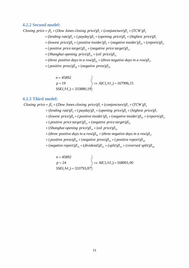
4.2.2 Second model: ...................................................................................................................... 11
4.2.3 Third model: ......................................................................................................................... 11
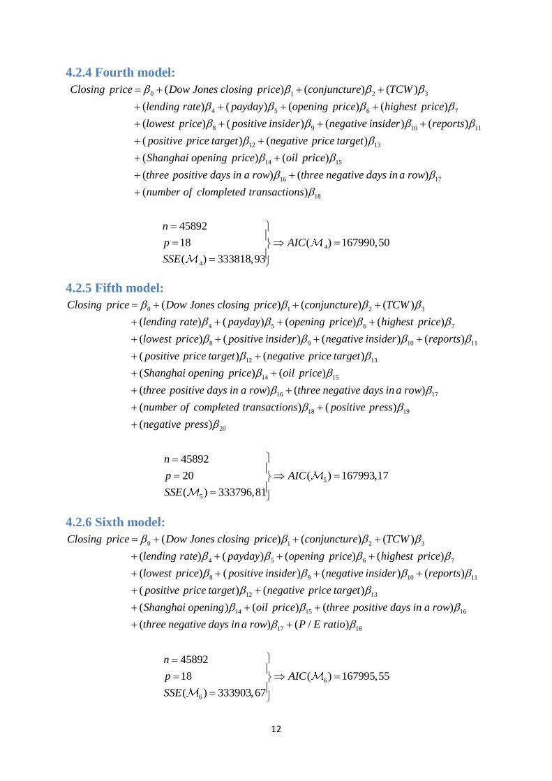
4.2.4 Fourth model: ....................................................................................................................... 12
4.2.5 Fifth model: .......................................................................................................................... 12
4.2.6 Sixth model: ......................................................................................................................... 12
4.2.7 Seventh model: ..................................................................................................................... 13
4.2 The final model ........................................................................................................................... 13
Chapter 5 Result .................................................................................................................................... 15
5.1 Plots of the residual and R2 value ................................................................................................ 15
5.2 Correct predicted directions ........................................................................................................ 16
5.3 Maximum and average deviation ................................................................................................ 17
5.4 Investing ...................................................................................................................................... 18
Chapter 6 Discussion ............................................................................................................................. 21
6.1 Discussion ................................................................................................................................... 21
Chapter 7 Appendix ............................................................................................................................... 23
7.1 Predicted closing price compared to real closing price ............................................................... 23
8.2 Yield using the model .................................................................................................................. 45
8.3 Stock exchange indexes ............................................................................................................... 67
8.4 Conjuncture ................................................................................................................................. 68
8.5 Oil price per barrel ...................................................................................................................... 69
8.6 TCW index .................................................................................................................................. 69
8.7 MATLAB code............................................................................................................................ 70
Chapter 9 References ............................................................................................................................. 91
9.1 References ................................................................................................................................... 91

1
Chapter 1 Introduction
1.1 Introduction Most people around the world dream of having more money in their pockets. The trick,
however, is not to work harder, but to work smarter. One way to make more money is to
invest on the stock exchange, but due to its seemingly random and unpredictable nature,
people are reluctant to do so. At first glance the stock exchange may seem random and
unpredictable, but that is not the entire truth. If the stock exchange is carefully analysed a
pattern will slowly emerge and it will be evident that there are a number of variables that
contributes to a company’s share price. Such variables are positive and negative news, price
target, conjuncture, oil price and other economic influential country’s stock exchange just to
name a few.
One of the most common share analysis tool used today is the so called regression channel.
These regression models are often sole based on the closing price vs. time and is more
reminiscent of a technical analysis rather than a prediction of the shares closing price. This
project aims to take it a step further by predicting a closing price for each day. The approach
is to determine which variables that has an influence on company’s share price, design a
multiple linear regression model and perform prediction using Microsoft Excel 2010’s[18]
built-in function LINEST to predict the closing price of 44 companies listed on the OMX
Stockholm stock exchange’s Large Cap list. The Large Cap list was at the time made up of 62
companies, but sufficient information was only found for 44 of them. Unlike the regression
channels that can be used for forecasting the direction of shares for several days ahead, even
weeks, this model will be used to analyse share prices on a daily basis for what resembles day
trading. The goal with the final model is to maximize the profit and minimize the losses based
on a daily analysis during the time period 2012-02-22 to 2013-02-20.
Since several multiple linear regression models were to be designed containing different sets
of covariates the Akaike Information Criterion (AIC) was used to determine the most suitable
model. One of the criterions for the model, set by us, were that it should be better than chance
in predicting if the share would increase or decrease in value i.e. have more than 50 % of the
predicted values in the correct direction. The other criterion was that the predicted closing
price should not deviate more than 10 % from the real closing price.
2
Chapter 2 Theory
2.1 Econometrics The term “econometrics” is believed to have been coined by the Norwegian man Ragnar
Frisch who lived between the years 1895-1973. He was one of the three principle founders of
the Econometric Society, first editor of the journal Econometrica and co-writer of the first
Nobel Memorial Prize in Economic Science in 1969[15]
.
Econometrics is used when it comes to applying statistical methods to problems when the data
available is observational rather than experimental, meaning the data obtained does not come
from controlled and planned experiments. Common fields where econometrics is applied are
economics, biology, medicine, social science and astronomy[16]
. The latter is a perfect
example of a natural science where data are typically observational and not experimental.
2.1.1 The Multiple Linear Regression Model theory
The basic model for econometric work and modelling for experimental design is the multiple
linear regression model[16]
. The specification is
(2.1)
where iy is the observation of the dependent random variable y whose expected value
depends on the covariates Cjx where C is a constant that denotes that i does not change. ie
represents the error terms and is assumed to be independent between observations and such
that
( |{ }) 0i jkE e x and 2 2( |{ })i jkE e x (2.2) (2.3)
where is unknown. Usually the covariate 0Cx is a constant 1 and 0 is the intercept.
If written
0( ... ), 1,...,i i ikx x x i n and 0( ... )T
k
then the specified model may be written as
i i iy x e (2.4)
The covariates may be deterministic (predetermined) values or outcomes of random
variables[16]
.
0
, 1,...,k
i ij j i
j
y x e i n

3
Sometimes it is convenient to use the matrix notation
Y X e where ( | ) 0E e X and 2( | )TE ee X I (2.5) (2.6)
where Y is a 1n -matrix of random variables, X is an ( 1)n k -matrix and e is an 1n -
matrix of random variables.
In the regression model above the parameters j and the variance 2 are unknown and it is
these parameters that are to be estimated from obtained data. The model can be used for either
prediction or it can be used to give a structural interpretation, which allows for hypotheses
testing. Since the project aims at predicting shares’ closing price the interesting part was
therefore only prediction.
2.2 Prediction When performing a prediction the linear model is often used
[16]. The covariates 0x makes up a
row matrix and with known covariates the predicted value of the corresponding ,y ,py is
0
ˆpy x . (2.7)
The prediction contains two unknown components; the estimated value of is used
instead of the real and the error term, which is set to zero in the prediction equation.
However, the error term is never zero in reality so to calculate it in the prediction the
following equation is used
0 0ˆ( )pe e x (2.8)
whose total variance is
1 2
0 0( ) (1 ( ) )T T
pVar e x X X x (2.9)
which is estimated to
1 2
0 0ˆ ( ) (1 ( ) )T T
pVar e x X X x s (2.10)
where s is an unbiased estimate of 2
2 21ˆ| |
1s e
n k
(2.11)

4
where n is the number of observations, k is the number of covariates in the prediction model
and 2 ˆˆ ˆ ˆ ˆ| | ,Te e e e Y X .
2.3 Regression channels On today’s stock exchange one of the most common analysis tools is the regression channel.
It uses historic values to forecast the future. The regression channel is based on a form of
chaos theory i.e. trying to predict something that springs from total chaos. A metaphoric
example can be made to illustrate how the regression channel works. Imagine a cigarette,
which stands straight up in a room where the air is perfectly still. The chaos theory says that
there is no way of predicting the smoke’s trails and loops as it leaves the cigarette. However,
if 10.000 cigarettes were to be observed in a row it would be noticed that the smoke trails of
one cigarette would never behave the same way as another cigarette’s, but at the same time it
would also be noticed that the smoke trails would never move outside a conical boundary on
their way up in the air. In chaos theory this boundary is known as a chaotic attractor.
Regression channels are based on the same principle, but instead of the smoke trail they use a
share’s closing price and the channel’s boundary is the chaotic attractor, which the share price
is not allowed to cross for a longer period of time. If the share moves outside the regression
channel it indicates that an unforeseen event has occurred, such as positive or negative news
or a new price target has been released and it is time to sell or buy the share.
One of the most common regression channels in use today is the Raff Regression Channel. It
uses time and closing price to draw up the channel. A regression line is created by analysing a
share’s closing price between certain days, say for example 100 days. Once the regression line
is drawn two more parallel lines are drawn, one above the regression line and one below it, at
equal distance from the regression line, see Figure 2.1. The distance is determined by the
highest or lowest share closing price from the regression line during the 100 days analysed[12]
.
The top line is seen as resistance and the bottom line is seen as support. The share may cross
these two lines for a short moment but if it stays outside for a longer period of time it
indicates that a new trend is coming.
5
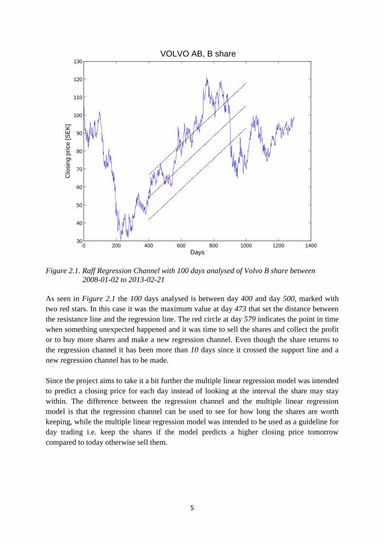
Figure 2.1. Raff Regression Channel with 100 days analysed of Volvo B share between
2008-01-02 to 2013-02-21
As seen in Figure 2.1 the 100 days analysed is between day 400 and day 500, marked with
two red stars. In this case it was the maximum value at day 473 that set the distance between
the resistance line and the regression line. The red circle at day 579 indicates the point in time
when something unexpected happened and it was time to sell the shares and collect the profit
or to buy more shares and make a new regression channel. Even though the share returns to
the regression channel it has been more than 10 days since it crossed the support line and a
new regression channel has to be made.
Since the project aims to take it a bit further the multiple linear regression model was intended
to predict a closing price for each day instead of looking at the interval the share may stay
within. The difference between the regression channel and the multiple linear regression
model is that the regression channel can be used to see for how long the shares are worth
keeping, while the multiple linear regression model was intended to be used as a guideline for
day trading i.e. keep the shares if the model predicts a higher closing price tomorrow
compared to today otherwise sell them.
0 200 400 600 800 1000 1200 140030
40
50
60
70
80
90
100
110
120
130C
losin
g p
rice [
SE
K]
Days
VOLVO AB, B share
6
Chapter 3 Data
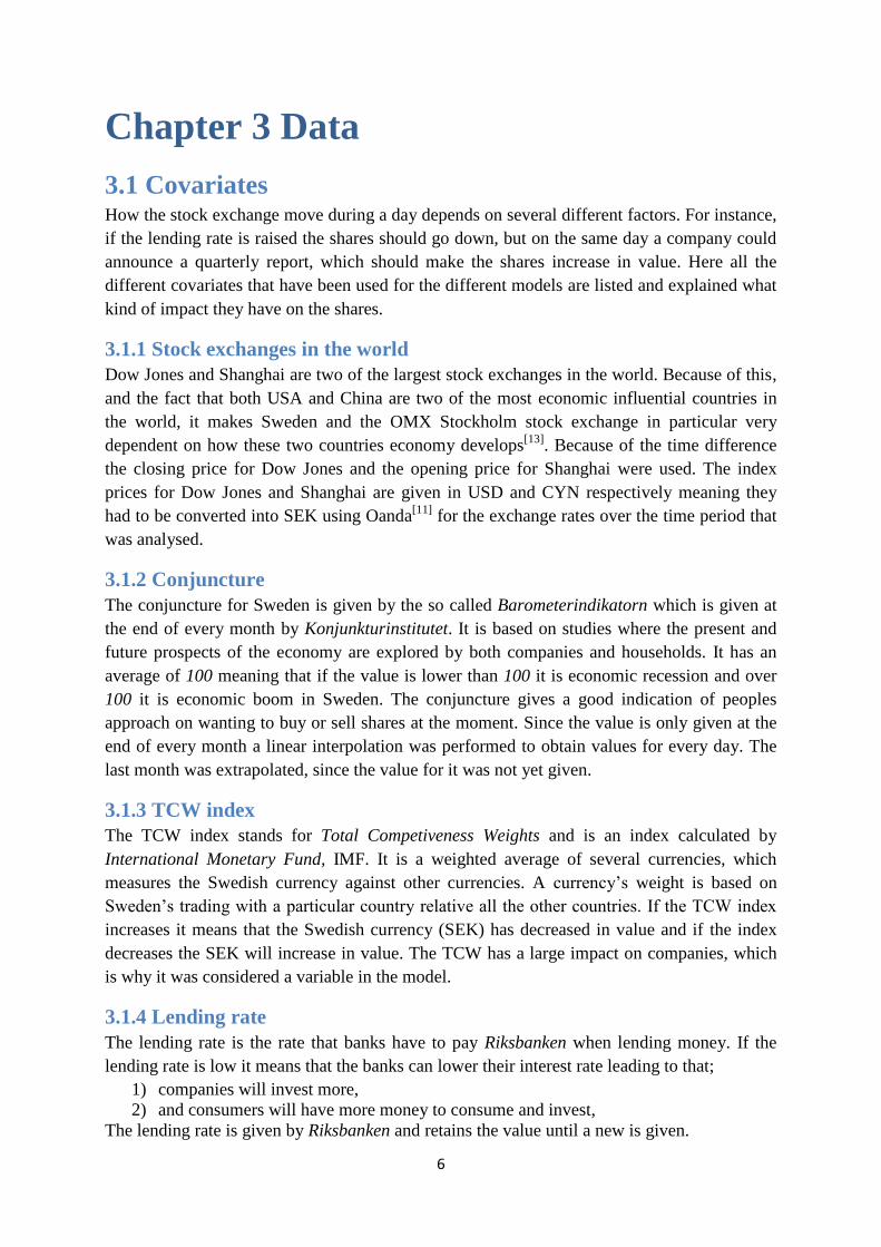
3.1 Covariates How the stock exchange move during a day depends on several different factors. For instance,
if the lending rate is raised the shares should go down, but on the same day a company could
announce a quarterly report, which should make the shares increase in value. Here all the
different covariates that have been used for the different models are listed and explained what
kind of impact they have on the shares.
3.1.1 Stock exchanges in the world
Dow Jones and Shanghai are two of the largest stock exchanges in the world. Because of this,
and the fact that both USA and China are two of the most economic influential countries in
the world, it makes Sweden and the OMX Stockholm stock exchange in particular very
dependent on how these two countries economy develops[13]
. Because of the time difference
the closing price for Dow Jones and the opening price for Shanghai were used. The index
prices for Dow Jones and Shanghai are given in USD and CYN respectively meaning they
had to be converted into SEK using Oanda[11]
for the exchange rates over the time period that
was analysed.
3.1.2 Conjuncture
The conjuncture for Sweden is given by the so called Barometerindikatorn which is given at
the end of every month by Konjunkturinstitutet. It is based on studies where the present and
future prospects of the economy are explored by both companies and households. It has an
average of 100 meaning that if the value is lower than 100 it is economic recession and over
100 it is economic boom in Sweden. The conjuncture gives a good indication of peoples
approach on wanting to buy or sell shares at the moment. Since the value is only given at the
end of every month a linear interpolation was performed to obtain values for every day. The
last month was extrapolated, since the value for it was not yet given.
3.1.3 TCW index
The TCW index stands for Total Competiveness Weights and is an index calculated by
International Monetary Fund, IMF. It is a weighted average of several currencies, which
measures the Swedish currency against other currencies. A currency’s weight is based on
Sweden’s trading with a particular country relative all the other countries. If the TCW index
increases it means that the Swedish currency (SEK) has decreased in value and if the index
decreases the SEK will increase in value. The TCW has a large impact on companies, which
is why it was considered a variable in the model.
3.1.4 Lending rate
The lending rate is the rate that banks have to pay Riksbanken when lending money. If the
lending rate is low it means that the banks can lower their interest rate leading to that;
1) companies will invest more,
2) and consumers will have more money to consume and invest,
The lending rate is given by Riksbanken and retains the value until a new is given.

7
3.1.5 Pay day
A dummy variable where a one indicated that salary was given on that day, normally on the
25th
every month. The hypothesis was that when people get their salary they might have some
extra money over after paying their bills, which could be used for investing in shares leading
to an increase in value.
3.1.6 Opening price
The opening price is the value that each share has when the OMX Stockholm stock exchange
opens for trading. The opening price gives a good indication of where the stock will move
during the day. Since the Stock exchange can be likened with an auction market i.e. buyers
and sellers meet to make deals with the highest bidder, the opening price does not have to be
the same as the last day’s closing price.
3.1.7 Highest/lowest price of the day
The highest and the lowest price of the day are taken the day before and gives an indication of
how much the shares usually move during a day and how this in the end will affect the closing
price. It also shows the general cyclical movement for each share.
3.1.8 Positive/Negative insider trading
Insider trading refers to trading done by people with good insight in how the company is
doing e.g. what kind of result they may present in the near future. People with good insight
could be the CEO, CEO of subsidiary, members of the board, people that own a lot of shares
in the company etc. This covariate was made up of two dummy variables; one for positive
insider trading where a one indicated that people with good insight in the company bought
shares, and one for negative insider trading where a one indicated that people with good
insight sold their shares. If people with good insight in the company sell their shares it might
indicate that the company is not doing as well as they thought and vice versa.
3.1.9 Quarterly and annual reports
The quarterly and annually reports are reports that present each company’s results for a
certain period. Usually when a company makes their reports public the share will increase in
value. This is often explained by the expectations that the investors have on the companies.
In this covariate only the release date was of interest i.e. the date that the report was released
so a dummy variable was created where a one indicated a released report.
3.1.10 Positive/negative price target
The price target is set by different analysts. Usually investors that do not have the time to
analyse the shares for themselves trust the analysts meaning that it gives a good indication of
when the shares will go up or down. The price target regards the share with the largest volume
i.e. the share that most people trade with, normally B shares. This covariate was made up of
two dummy variables; one for positive price target where a one indicated that the analysts
gave a price target larger than the actual price for the share and one for negative price target
where a one indicated that analysts gave a price target lower than the actual price for the
share.

8
3.1.11 Oil price
The oil price gives a good indication of how strong the USD is and the condition of the USD
has a big impact on the worldwide stock market. Since the oil price is given as USD/barrel it
was converted it into SEK/barrel to match the model. Another effect the oil price has on
shares is that if the oil price rises a company’s share value normally decreases since nearly
every company depends on oil for production[14]
. Therefore if the oil price rises the
company’s expenses increases and their profit will decrease.
3.1.12 Three positive/three negative days in a row
The hypothesis was that when a share moved in one direction for several days it would have a
big impact on peoples feeling toward the company. This covariate was made up of two
dummy variables; one for three positive days in a row where a one indicated that the share’s
closing price had increased in the last three days, and one for three negative days in a row
where a one indicated that the share had decreased in the last three days.
3.1.13 P/E ratio
This is a ratio calculated by
//
Current share priceP E
Earnings share (3.1)
and is a measurement of how long it will take to get the investment back, provided that the
earnings remain unchanged. The P/E-ratio is given in years. From where were the data was
collected the P/E-ratio was given once a year for each company so the values were linear
interpolated to obtain them for every day.
3.1.14 Positive/Negative press releases
Whenever a company makes a press release it will have an impact on their shares. These
releases can be about letting people go or that the company has just made a huge profitable
deal. This covariate was made up of two dummy variables; one for positive press releases
where a one indicated that a positive release had been made, and one for negative press
releases where a one indicated that a negative release had been made.
3.1.15 Number of completed transactions
This is the number of completed trading transactions that has been done with a company’s
share during one day. This number usually increases when a report is about to be released. It
gives a good indication of how popular a company’s shares are at the moment.
3.1.16 OMX Stockholm closing price
This is the value of how the total OMX Stockholm exchange has moved during the day.
3.1.17 Split and reversed split
A split is when a share is divided into several others and reverse is when several shares are
made into one. This covariate was made up of two dummy variables; one for split where a one

9
indicated a split had been made and one for reversed split where a one indicated a reversed
split had been made.
3.2 Collecting data The historical data for all of the shares and the press releases was collected from
Nasdaqomxnordic[1] [2]
The data for the conjuncture and TCW index was collected from Ekonomifakta[4] [6]
.
The index for Dow Jones was collected from Stloisfed[8]
and for Shanghai from Yahoo
finance[9]
.
The insider trading was collected from Finansinstitutionen[5]
Target prices and P/E-ratio was both found at Dagens ndustry[3]
The Oil price per barrel was collected from Eia[10]
The lending rate was collected from Riksbanken[7]
All of the exchange rates for converting foreign currencies into SEK was collected from
Oanda[11]
The data was then processed in Microsoft Excel 2010[18]
using its built-in function LINEST to
make the regression. For making the plots MATLAB[17]
and Minitab 16[19]
was used.
Chapter 4 Modelling
4.1 Modelling Before designing the multiple linear regression models a number of covariates had to be
evaluated to see what kind of impact they had on the share prices. The modelling process
consisted of testing different types of covariate combinations until a satisfactory result had
been achieved. What was learned during the modelling process was that theory put into
practice does not always yield a perfect result. Covariate combinations that should have
yielded a better result sometimes turned out to be worse. When seven satisfactory multiple
linear regression models had been designed Akaike’s Information Criterion, AIC, was applied
to determine which model that was most suitable.
4.2 AIC test Since multiple linear regression modelling often results in several different model designs it is
important to choose the best model suitable. One way of settling for a model is to use
Akaike’s Information Criterion, AIC. The AIC provides an index that can be used to

10
determine which of several competing models to go with. The multiple linear regression
model with the lowest AIC index should be the model of choice.
The general formula for AIC is
) 2 log( ( ) 2 ( )( )i i iAIC L p (4.1)
where ( )iL is the likelihood function of the parameters in model i evaluated at the
maximum likelihood estimators and p is the number of covariates in the model. According to
stat.stanford[20]
the general formula can rewritten as
) (log(2 ) log( ( )) log( )) 2 ( 1)( n SSE nAI pC n (4.2)
where stands for the model that is tested, n is number of observations, p number of
covariates and SSE is the sum squared error. The models that were tested and their AIC
indexes were the following.
4.2.1 First model
0 1 2 3
4 5 6 7
8 9 10 11
( ) ( ) ( )
( ) ( ) ( ) ( )
( ) ( ) ( ) ( )
(
Closing price Dow Jones closing price conjuncture TCW
lending rate payday opening price highest price
lowest price positive insider negative insider reports
pos
12 13
14 15
16 17
) ( )
( ) ( )
( ) ( )
itive price target negative price target
Shanghai opening price oil price
three positive days in a row three negative days in a row
1
1
( ) 167993,61
) 333904,69
45892
17
(
AIC
n
p
SSE
11
4.2.2 Second model:
0 1 2 3
4 5 6 7
8 9 10 11
( ) ( ) ( )
( ) ( ) ( ) ( )
( ) ( ) ( ) ( )
(
Closing price Dow Jones closing price conjuncture TCW
lending rate payday opening price highest price
lowest price positive insider negative insider reports
pos
12 13
14 15
16 17
18 19
) ( )
( ) ( )
( ) ( )
( ) ( )
itive price target negative price target
Shanghai opening price oil price
three positive days in a row three negative days in a row
positive press negative press
2
2
( ) 167996,15
) 333880,19
45892
19
(
AIC
n
p
SSE
4.2.3 Third model:
0 1 2 3
4 5 6 7
8 9 10 11
( ) ( ) ( )
( ) ( ) ( ) ( )
( ) ( ) ( ) ( )
(
Closing price Dow Jones closing price conjuncture TCW
lending rate payday opening price highest price
lowest price positive insider negative insider reports
pos
12 13
14 15
16 17
18 19 2
) ( )
( ) ( )
( ) ( )
( ) ( ) ( )
itive price target negative price target
Shanghai opening price oil price
three positive days in a row three negative days in a row
positive press negative press positive report
0
21 22 23 24( ) ( ) ( ) ( )negative report dividend split reversed split
3
3
( ) 168001,00
) 333793,87
45892
24
(
AIC
n
p
SSE
12
4.2.4 Fourth model:
0 1 2 3
4 5 6 7
8 9 10 11
( ) ( ) ( )
( ) ( ) ( ) ( )
( ) ( ) ( ) ( )
(
Closing price Dow Jones closing price conjuncture TCW
lending rate payday opening price highest price
lowest price positive insider negative insider reports
pos
12 13
14 15
16 17
18
) ( )
( ) ( )
( ) ( )
( )
itive price target negative price target
Shanghai opening price oil price
three positive days in a row three negative days in a row
number of clompleted transactions
4
4
( ) 167990,50
) 333818,93
45892
18
(
AIC
n
p
SSE
4.2.5 Fifth model:
0 1 2 3
4 5 6 7
8 9 10 11
( ) ( ) ( )
( ) ( ) ( ) ( )
( ) ( ) ( ) ( )
(
Closing price Dow Jones closing price conjuncture TCW
lending rate payday opening price highest price
lowest price positive insider negative insider reports
pos
12 13
14 15
16 17
18 19
) ( )
( ) ( )
( ) ( )
( ) ( )
(
itive price target negative price target
Shanghai opening price oil price
three positive days in a row three negative days in a row
number of completed transactions positive press
n
20)egative press
5
5
( ) 167993,17
) 333796,81
45892
20
(
AIC
n
p
SSE
4.2.6 Sixth model:
0 1 2 3
4 5 6 7
8 9 10 11
( ) ( ) ( )
( ) ( ) ( ) ( )
( ) ( ) ( ) ( )
(
Closing price Dow Jones closing price conjuncture TCW
lending rate payday opening price highest price
lowest price positive insider negative insider reports
pos
12 13
14 15 16
17 18
) ( )
( ) ( ) ( )
( ) ( / )
itive price target negative price target
Shanghai opening oil price three positive days in a row
three negative days in a row P E ratio
6
6
( ) 167995,55
) 333903,67
45892
18
(
AIC
n
p
SSE

13
4.2.7 Seventh model:
0 1 2 3
4 5 6 7
8 9 10 11
( ) ( ) ( )
( ) ( ) ( ) ( )
( ) ( ) ( ) ( )
(
Closing price Dow Jones closing price conjuncture TCW
lending rate payday opening price highest price
lowest price positive insider negative insider reports
pos
12 13
14 15
16 17
18
) ( )
( ) ( )
( ) ( )
( )
(
itive price target negative price target
Shanghai opening price oil price
three positive days in a row three negative days in a row
number of completed transactions
OMX Stockholm opening p
19)rice
7
7
( ) 167929,88
) 332771,86
45892
19
(
AIC
n
p
SSE
Summary of the AIC indexes were as follows.
1( )AIC 2( )AIC 3( )AIC 4( )AIC 5( )AIC 6( )AIC 7( )AIC
167993,61 167996,15 168001,00 167990,50 167993,17 167995,55 167929,88
As mentioned above the model with the lowest AIC index should be the best model of choice.
Here the multiple linear regression model with the lowest AIC index is number seven hence
the model to go with.
4.2 The final model
The aim was to create a general multiple linear regression model that could be applied to all
44 shares analysed. To achieve this four years (2008-01-02 to 2012-02-21) of data from every
share was collected and inserted into a single Microsoft Excel 2010[18]
sheet. The amount of
data made up 45892 observations. Microsoft Excel 2010’s built-in function LINEST was used
to perform the regression. The LINEST-function gives the i :s value and the corresponding
error term for every covariate used. The final model that was used had the following design.
0 1 2 3
4 5 6 7
8 9 10 11
( ) ( ) ( )
( ) ( ) ( ) ( )
( ) ( ) ( ) ( )
(
Closing price Dow Jones closing price conjuncture TCW
interest rate payday opening price highest value
lowest value positive insider negative insider reports
po
12 13
14 15
16 17
18
) ( )
( ) ( )
( ) ( )
( )
(
sitive price target negativ price target
Shanghai opening price oil price
three positive days in a row three negative days in a row
number of completed transactions
OMX Stockholm opening p
19)rice

14
i -values corresponding residuals, ie
β0 7,33539 e0 1,00779
β1 1,4295 10-5
e1 3,62151 10-6
β2 0,01035 e2 0,00240
β3 – 0,04664 e3 0,005639
β4 – 0,24109 e4 0,01902
β5 0,25977 e5 0,06065
β6 0,96488 e6 0,00398
β7 – 0,04321 e7 0,00652
β8 0,07893 e8 0,00659
β9 0,04293 e9 0,06880
β10 0,06856 e10 0,11282
β11 0,26392 e11 0,09203
β12 – 0,09910 e12 0,05644
β13 – 0,16703 e13 0,09102
β14 0,00024 e14 3,48251 10-5
β15 0,00076 e15 0,00020
β16 0,02782 e16 0,04033
β17 0,08593 e17 0,03795
β18 1,3626 10-5
e18 5,17749 10-6
β19 – 0,00433 e19 0,99883
Table 4.1. β-values and corresponding residuals from the regression of the final model
(2008-01-02 to 2012-02-21).
The i :s where then used to calculate the estimated y (closing price) by the formula
19,192,21,10 ...ˆ jjj xxxy (4.3)
where j denotes the jth
row i.e. jth
day predicted in Microsoft Excel 2010[18]
.
15
Chapter 5 Result
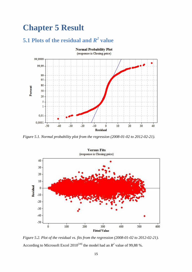
5.1 Plots of the residual and R2 value
Figure 5.1. Normal probability plot from the regression (2008-01-02 to 2012-02-21).
Figure 5.2. Plot of the residual vs. fits from the regression (2008-01-02 to 2012-02-21).
According to Microsoft Excel 2010[18]
the model had an R2 value of 99,88 %.
16
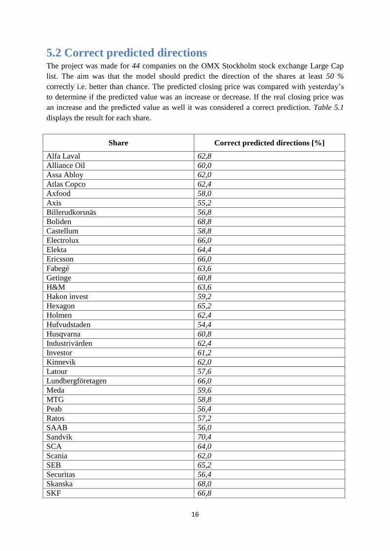
5.2 Correct predicted directions The project was made for 44 companies on the OMX Stockholm stock exchange Large Cap
list. The aim was that the model should predict the direction of the shares at least 50 %
correctly i.e. better than chance. The predicted closing price was compared with yesterday’s
to determine if the predicted value was an increase or decrease. If the real closing price was
an increase and the predicted value as well it was considered a correct prediction. Table 5.1
displays the result for each share.
Share Correct predicted directions [%]
Alfa Laval 62,8
Alliance Oil 60,0
Assa Abloy 62,0
Atlas Copco 62,4
Axfood 58,0
Axis 55,2
Billerudkorsnäs 56,8
Boliden 68,8
Castellum 58,8
Electrolux 66,0
Elekta 64,4
Ericsson 66,0
Fabegé 63,6
Getinge 60,8
H&M 63,6
Hakon invest 59,2
Hexagon 65,2
Holmen 62,4
Hufvudstaden 54,4
Husqvarna 60,8
Industrivärden 62,4
Investor 61,2
Kinnevik 62,0
Latour 57,6
Lundbergföretagen 66,0
Meda 59,6
MTG 58,8
Peab 56,4
Ratos 57,2
SAAB 56,0
Sandvik 70,4
SCA 64,0
Scania 62,0
SEB 65,2
Securitas 56,4
Skanska 68,0
SKF 66,8
17
SSAB 62,4
Swedbank 62,4
Swedish Match 58,4
TeliaSonera 58,8
Trelleborg 66,4
Volvo 70,8
Wallenstam 55,2
Table 5.1. Correct predicted directions in percentage for each share
(2012-02-22 to 2013-02-20).
Each share was over 50 % which was the project aim, meaning that the model is profitable on
a day by day basis in the long term. Since the model is intended to be applicable on all shares
an average correct predicted direction was calculated
Average correct predicted direction = 62,8 60,0 ... 55,2
61,71%44
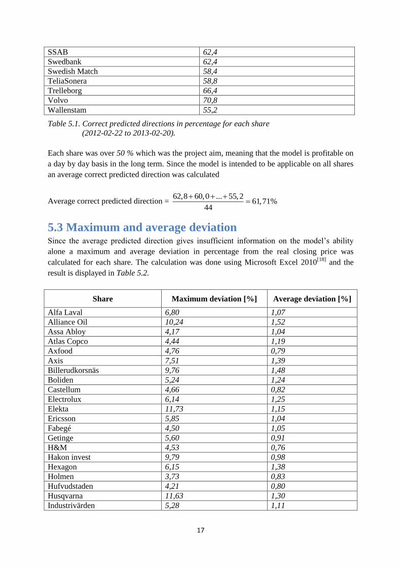
5.3 Maximum and average deviation Since the average predicted direction gives insufficient information on the model’s ability
alone a maximum and average deviation in percentage from the real closing price was
calculated for each share. The calculation was done using Microsoft Excel 2010[18]
and the
result is displayed in Table 5.2.
Share Maximum deviation [%] Average deviation [%]
Alfa Laval 6,80 1,07
Alliance Oil 10,24 1,52
Assa Abloy 4,17 1,04
Atlas Copco 4,44 1,19
Axfood 4,76 0,79
Axis 7,51 1,39
Billerudkorsnäs 9,76 1,48
Boliden 5,24 1,24
Castellum 4,66 0,82
Electrolux 6,14 1,25
Elekta 11,73 1,15
Ericsson 5,85 1,04
Fabegé 4,50 1,05
Getinge 5,60 0,91
H&M 4,53 0,76
Hakon invest 9,79 0,98
Hexagon 6,15 1,38
Holmen 3,73 0,83
Hufvudstaden 4,21 0,80
Husqvarna 11,63 1,30
Industrivärden 5,28 1,11

18
Investor 4,02 0,83
Kinnevik 6,82 0,83
Latour 5,42 1,19
Lundbergföretagen 4,66 0,82
Meda 4,81 0,85
MTG 29,19 1,47
Peab 5,59 1,36
Ratos 8,81 1,38
SAAB 4,52 1,09
Sandvik 6,27 1,21
SCA 8,10 0,88
Scania 5,11 1,20
SEB 4,68 1,09
Securitas 4,99 1,04
Skanska 3,47 0,82
SKF 8,48 1,10
SSAB 5,57 1,56
Swedbank 5,31 1,01
Swedish Match 6,72 0,91
TeliaSonera 3,78 0,76
Trelleborg 7,02 1,27
Volvo 5,80 1,20
Wallenstam 4,33 1,11
Table 5.2. Maximum and average deviation in percentage for each share (2012-02-22 to
2013-02-20).
The average maximum deviation was 6,60 % and the average deviation was 1,03 %.
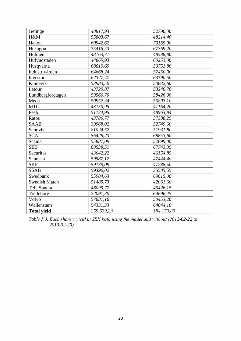
5.4 Investing To evaluate the model further an investment test was conducted. If 50.000 SEK had been
invested in each share, a total investment of 2.2 million SEK, and the model had been applied
over the year 2012-02-22 to 2013-02-20 the total yield would have been 259.639 SEK
corresponding to 11,8 %. If the same investment had been done and the shares were never to
be traded with during the same period of time i.e. the investment would have been done at
2012-02-22 and then sold at 2013-02-20, the total yield would have been 184.171 SEK
corresponding to 8,37 %. This means that the model would have generated a 40,98 % greater
yield that year. In Table 5.3 the shares’ result after a year is presented both using the model
and without.
To calculate each share’s yield Microsoft Excel 2010[18]
was used. First a prediction column
was created were a one indicated that the predicted closing price would be higher than
yesterday’s real closing price, if the predicted value was lower or equal to yesterday’s real
closing price a zero was shown. The four red columns to the right of the prediction column
indicates if the prediction column goes from zero to one, one to one, one to zero or zero to
zero. Each day there was a one present in the zero to one column shares was bought to the real
opening price. Each day there was a one present in the one to one column the shares bought

19
earlier were kept and the profit/loss was added to yesterday’s daily value. Each day there was
a one present in the one to zero column the shares were sold to the real opening price. Each
day there was a one present in the zero to zero column nothing happened since the share was
not of interest. To get an overview of how the calculation was made see Figure 5.3.
Figure 5.3. Extract of how the calculations of Sandvik’s yield was made in Microsoft Excel
2010[18]
using the model (2012-02-22 to 2013-02-20)
Share
How much the investment
of 50.000 SEK is worth
after the year using the
model [SEK]
How much the investment
of 50.000 SEK is worth
after the year not using the
model [SEK]
Alfa Laval 59970,21 55875,00
Alliance Oil 44225,26 33261,30
Assa Abloy 58206,55 63075,00
Atlas Copco 59086,73 53941,30
Axfood 45873,00 55540,80
Axis 42776,07 44362,50
Billeurdkorsnäs 46192,24 52641,75
Boliden 67020,51 47523,00
Castellum 52277,52 55265,85
Electrolux 68260,31 57024,00
Elekta 64516,28 64085,40
Ericsson 57895,17 59969,40
Fabege 59531,77 60455,25
20
Getinge 48817,93 52796,00
H&M 55803,67 48214,40
Hakon 60942,62 79165,00
Hexagon 75416,53 67369,20
Holmen 43163,71 48588,80
Hufvudstaden 44869,93 60253,00
Husqvarna 68619,69 50751,80
Industrivärden 64668,24 57450,00
Investor 62327,47 63790,50
Kinnevik 53983,50 50832,60
Latour 43729,87 53246,70
Lundbergföretagen 59566,70 58426,00
Meda 50952,34 55803,10
MTG 43150,95 41164,20
Peab 51134,95 48963,84
Ratos 43780,77 37388,25
SAAB 39568,02 52749,60
Sandvik 81024,52 51931,80
SCA 56428,23 68853,60
Scania 55887,09 52899,00
SEB 68538,51 67743,35
Securitas 43642,22 46154,85
Skanska 59587,12 47444,40
SKF 59139,09 47288,50
SSAB 59390,02 35585,55
Swedbank 55984,63 69615,00
Swedish Match 51485,73 42061,60
TeliaSonera 48099,77 45426,15
Trelleborg 72091,30 64696,25
Volvo 57681,16 50453,20
Wallenstam 54331,33 64044,10
Total yield 259.639,23 184.170,89
Table 5.3. Each share’s yield in SEK both using the model and without (2012-02-22 to
2013-02-20).
21
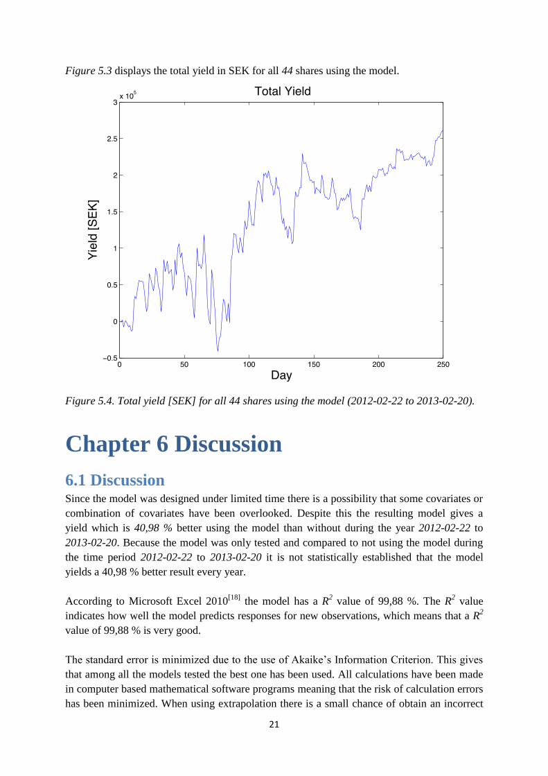
Figure 5.3 displays the total yield in SEK for all 44 shares using the model.
Figure 5.4. Total yield [SEK] for all 44 shares using the model (2012-02-22 to 2013-02-20).
Chapter 6 Discussion
6.1 Discussion Since the model was designed under limited time there is a possibility that some covariates or
combination of covariates have been overlooked. Despite this the resulting model gives a
yield which is 40,98 % better using the model than without during the year 2012-02-22 to
2013-02-20. Because the model was only tested and compared to not using the model during
the time period 2012-02-22 to 2013-02-20 it is not statistically established that the model
yields a 40,98 % better result every year.
According to Microsoft Excel 2010[18]
the model has a R2 value of 99,88 %. The R
2 value
indicates how well the model predicts responses for new observations, which means that a R2
value of 99,88 % is very good.
The standard error is minimized due to the use of Akaike’s Information Criterion. This gives
that among all the models tested the best one has been used. All calculations have been made
in computer based mathematical software programs meaning that the risk of calculation errors
has been minimized. When using extrapolation there is a small chance of obtain an incorrect

22
result. However the difference between the extrapolated value and the real is small and it will
only affect the predicted value with approximately 0,1-0,2 SEK. The reason for linear
interpolation of the conjuncture was since the values were only given once a month they had
to be linear between two months.
The reason for designing a general model was because of the fact that it is intended to be used
as a day trading guideline in the mornings when the opening price is known. It is of great
importance that the calculations can be completed quickly so that decisions regarding selling
or buying shares can be done fast. This is where the general model has an advantage
compared to several tailor made models. Security is found in numbers when it comes to share
trading.
Four years (2008-01-02 to 2012-02-21) of data from every share was collected and inserted
into a single Microsoft Excel 2010[18]
sheet. The amount of data made up 45892 observations.
Microsoft Excel 2010’s[18]
built-in function LINEST was used to perform the regression. The
LINEST-function gives the i :s value and the corresponding error term for every covariate
used. The data was collected for four years due to the fact that more observations lead to a
better reliability of the model. Another reason was to include the worldwide stock market
crash of 2008. The β-values of the model will then be more accurate towards TCW index,
conjuncture, oil price, Dow Jones index, Shanghai index and OMX Stockholm index which
make the model more reliable.
Another approach to predict share’s closing price is to use Markov processes. Unlike multiple
linear regression which analyses historical data the Markov process uses the present to predict
the future. Since shares are memoryless i.e. they are not affected by yesterday’s cyclic
movement, it is possible that Markov processes would have yielded a better result. The reason
why multiple linear regression yields such a good result after all could be that four years of
historical data from 44 shares displays people’s irrational behaviour which is the main reason
why shares are considered random and unpredictable.
23
Chapter 7 Appendix
7.1 Predicted closing price compared to real closing price
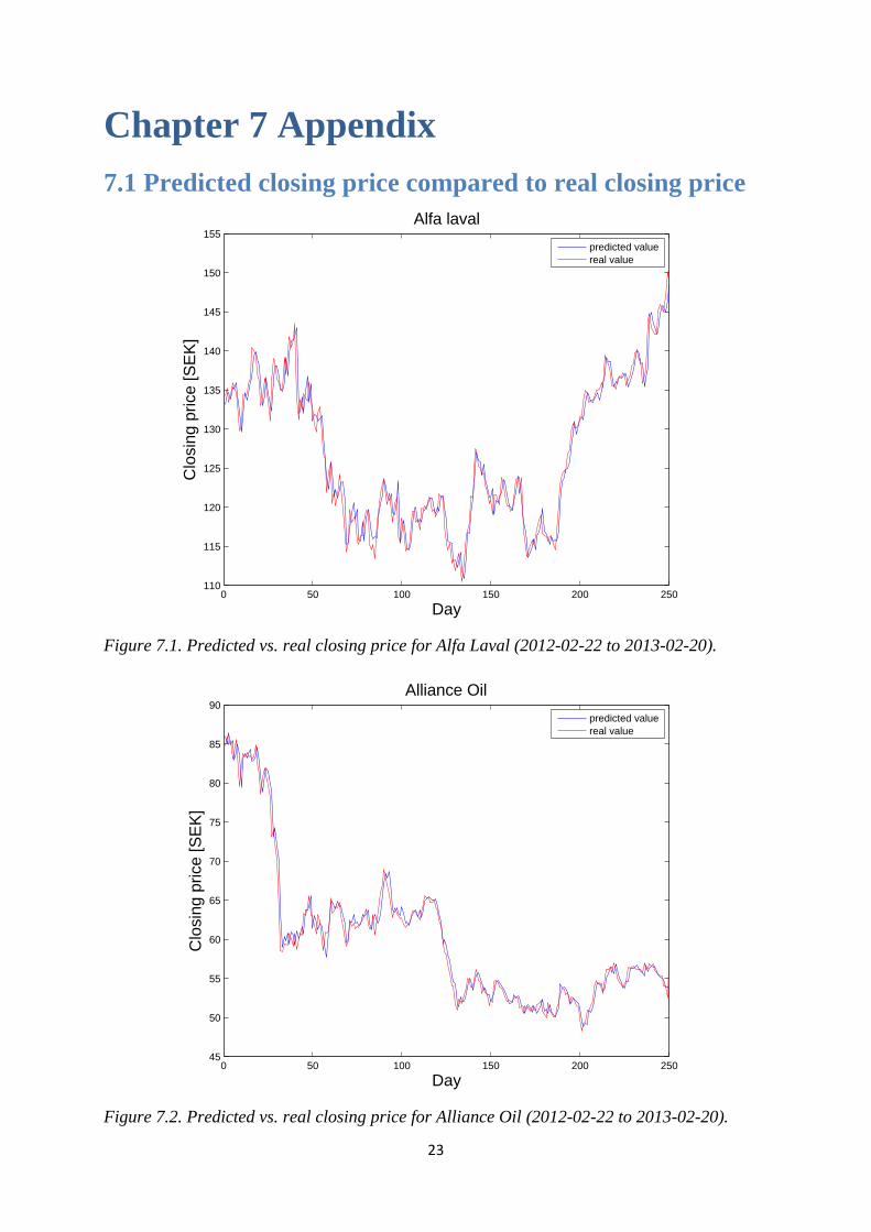
Figure 7.1. Predicted vs. real closing price for Alfa Laval (2012-02-22 to 2013-02-20).
Figure 7.2. Predicted vs. real closing price for Alliance Oil (2012-02-22 to 2013-02-20).
0 50 100 150 200 250110
115
120
125
130
135
140
145
150
155
Alfa laval
Day
Clo
sin
g p
rice
[S
EK
]
predicted value
real value
0 50 100 150 200 25045
50
55
60
65
70
75
80
85
90
Alliance Oil
Day
Clo
sin
g p
rice
[S
EK
]
predicted value
real value
24
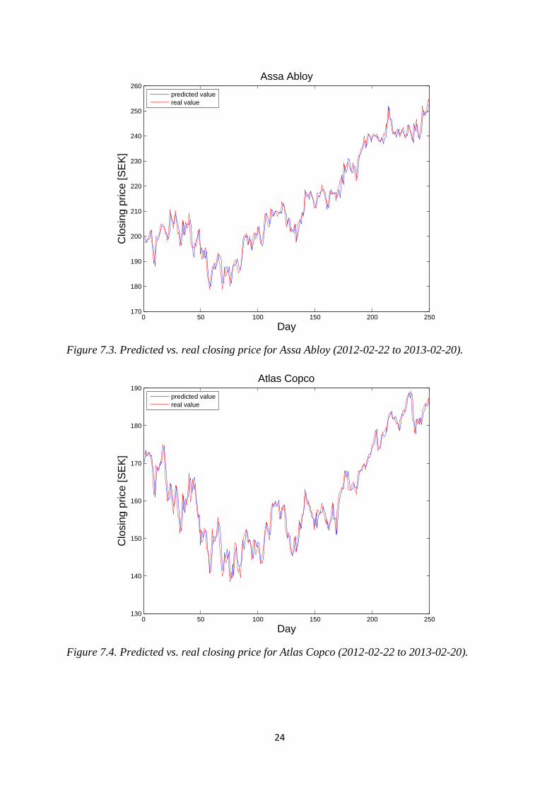
Figure 7.3. Predicted vs. real closing price for Assa Abloy (2012-02-22 to 2013-02-20).
Figure 7.4. Predicted vs. real closing price for Atlas Copco (2012-02-22 to 2013-02-20).
0 50 100 150 200 250170
180
190
200
210
220
230
240
250
260
Assa Abloy
Day
Clo
sin
g p
rice
[S
EK
]
predicted value
real value
0 50 100 150 200 250130
140
150
160
170
180
190
Atlas Copco
Day
Clo
sin
g p
rice
[S
EK
]
predicted value
real value
25
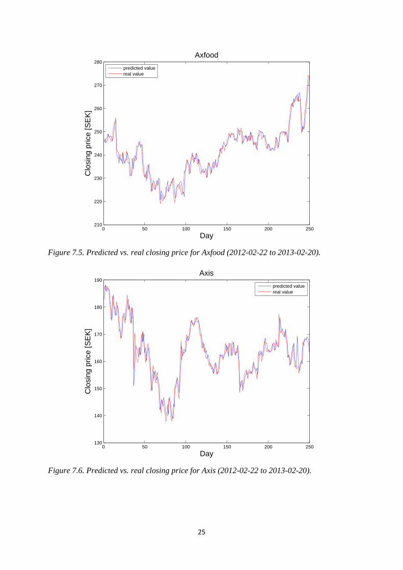
Figure 7.5. Predicted vs. real closing price for Axfood (2012-02-22 to 2013-02-20).
Figure 7.6. Predicted vs. real closing price for Axis (2012-02-22 to 2013-02-20).
0 50 100 150 200 250210
220
230
240
250
260
270
280
Axfood
Day
Clo
sin
g p
rice
[S
EK
]
predicted value
real value
0 50 100 150 200 250130
140
150
160
170
180
190
Axis
Day
Clo
sin
g p
rice
[S
EK
]
predicted value
real value
26
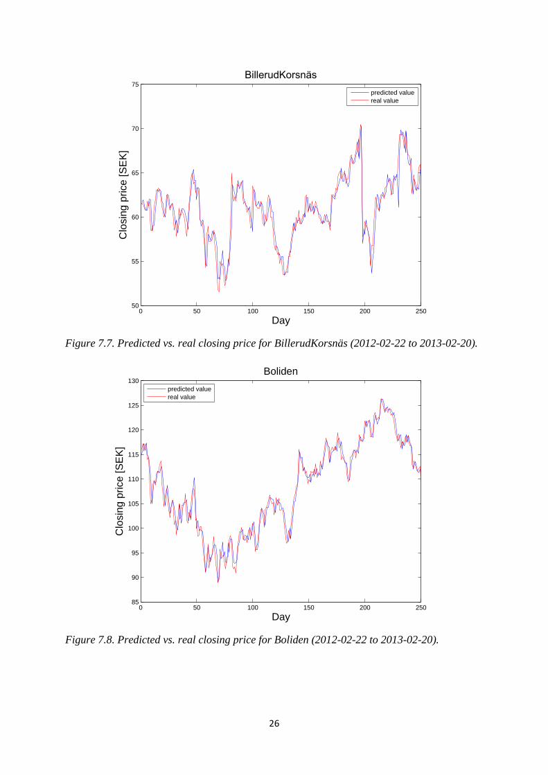
Figure 7.7. Predicted vs. real closing price for BillerudKorsnäs (2012-02-22 to 2013-02-20).
Figure 7.8. Predicted vs. real closing price for Boliden (2012-02-22 to 2013-02-20).
0 50 100 150 200 25050
55
60
65
70
75
BillerudKorsnäs
Day
Clo
sin
g p
rice
[S
EK
]
predicted value
real value
0 50 100 150 200 25085
90
95
100
105
110
115
120
125
130
Boliden
Day
Clo
sin
g p
rice
[S
EK
]
predicted value
real value

27
Figure 7.9. Predicted vs. real closing price for Castellum (2012-02-22 to 2013-02-20).
Figure 7.10. Predicted vs. real closing price for Electrolux (2012-02-22 to 2013-02-20).
0 50 100 150 200 25075
80
85
90
95
100
Castellum
Day
Clo
sin
g p
rice
[S
EK
]
predicted value
real value
0 50 100 150 200 250120
130
140
150
160
170
180
Electrolux
Day
Clo
sin
g p
rice
[S
EK
]
predicted value
real value
28
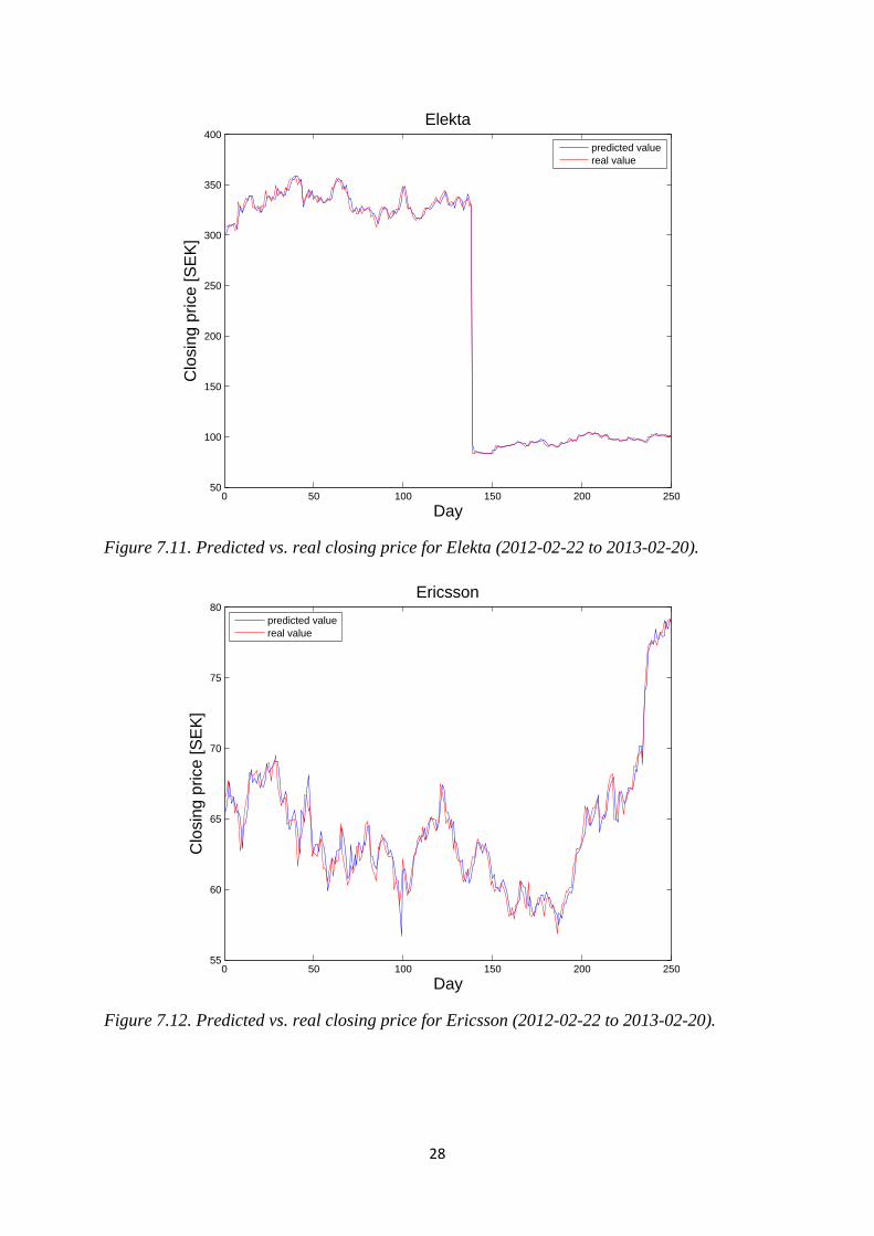
Figure 7.11. Predicted vs. real closing price for Elekta (2012-02-22 to 2013-02-20).
Figure 7.12. Predicted vs. real closing price for Ericsson (2012-02-22 to 2013-02-20).
0 50 100 150 200 25050
100
150
200
250
300
350
400
Elekta
Day
Clo
sin
g p
rice
[S
EK
]
predicted value
real value
0 50 100 150 200 25055
60
65
70
75
80
Ericsson
Day
Clo
sin
g p
rice
[S
EK
]
predicted value
real value
29
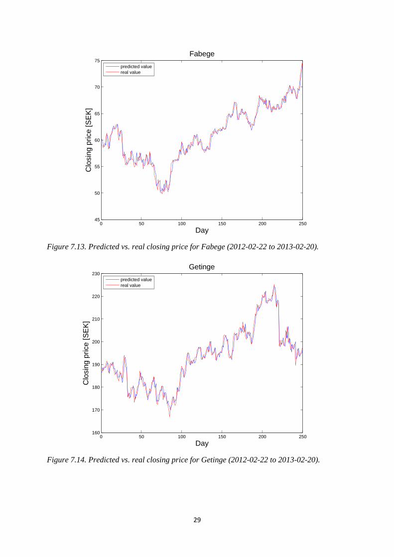
Figure 7.13. Predicted vs. real closing price for Fabege (2012-02-22 to 2013-02-20).
Figure 7.14. Predicted vs. real closing price for Getinge (2012-02-22 to 2013-02-20).
0 50 100 150 200 25045
50
55
60
65
70
75
Fabege
Day
Clo
sin
g p
rice
[S
EK
]
predicted value
real value
0 50 100 150 200 250160
170
180
190
200
210
220
230
Getinge
Day
Clo
sin
g p
rice
[S
EK
]
predicted value
real value
30
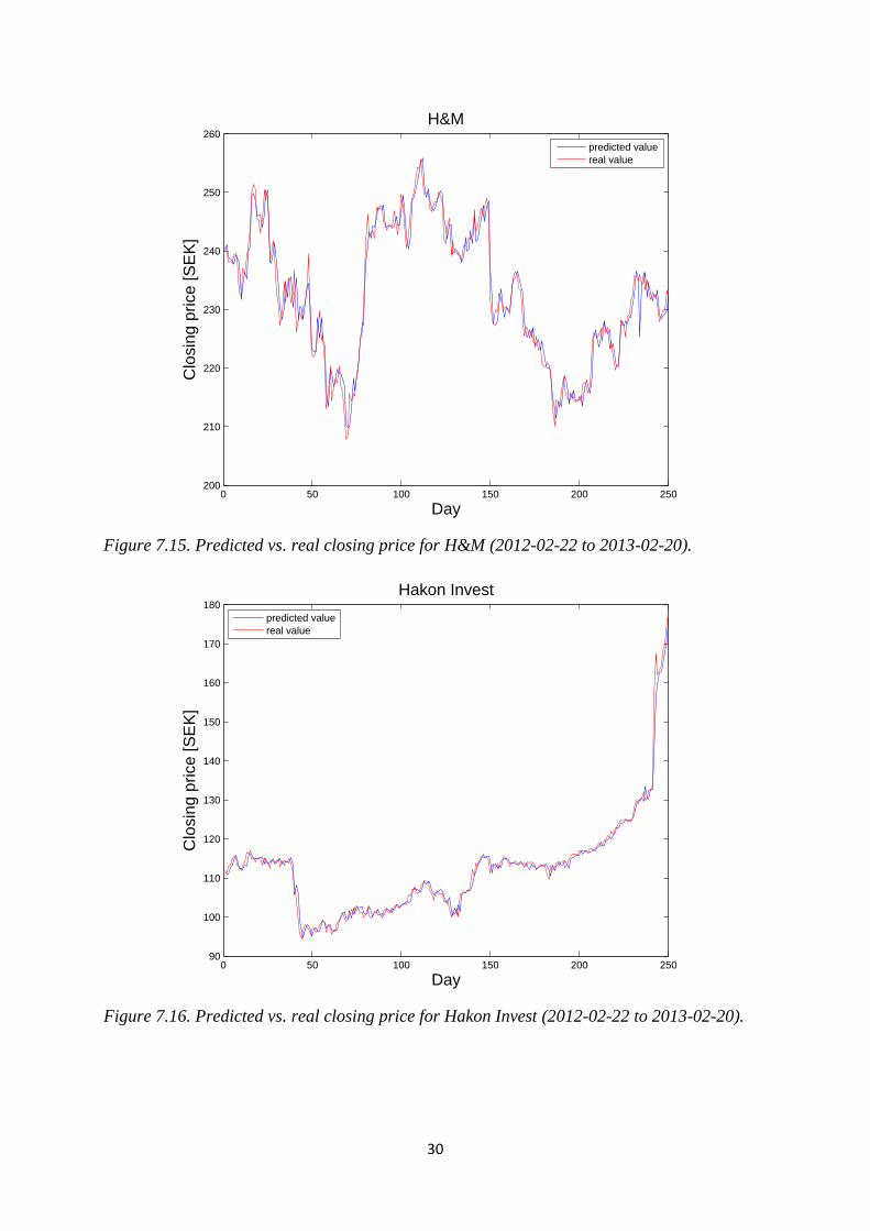
Figure 7.15. Predicted vs. real closing price for H&M (2012-02-22 to 2013-02-20).
Figure 7.16. Predicted vs. real closing price for Hakon Invest (2012-02-22 to 2013-02-20).
0 50 100 150 200 250200
210
220
230
240
250
260
H&M
Day
Clo
sin
g p
rice
[S
EK
]
predicted value
real value
0 50 100 150 200 25090
100
110
120
130
140
150
160
170
180
Hakon Invest
Day
Clo
sin
g p
rice
[S
EK
]
predicted value
real value
31
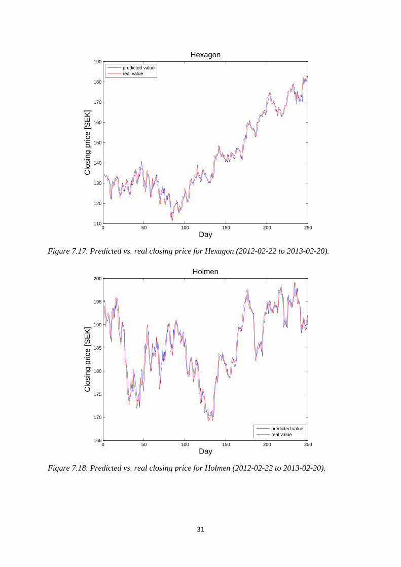
Figure 7.17. Predicted vs. real closing price for Hexagon (2012-02-22 to 2013-02-20).
Figure 7.18. Predicted vs. real closing price for Holmen (2012-02-22 to 2013-02-20).
0 50 100 150 200 250110
120
130
140
150
160
170
180
190
Hexagon
Day
Clo
sin
g p
rice
[S
EK
]
predicted value
real value
0 50 100 150 200 250165
170
175
180
185
190
195
200
Holmen
Day
Clo
sin
g p
rice
[S
EK
]
predicted value
real value
32
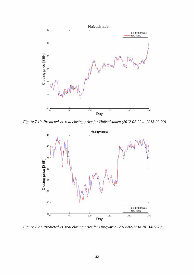
Figure 7.19. Predicted vs. real closing price for Hufvudstaden (2012-02-22 to 2013-02-20).
Figure 7.20. Predicted vs. real closing price for Husqvarna (2012-02-22 to 2013-02-20).
0 50 100 150 200 25065
70
75
80
85
90
95
Hufvudstaden
Day
Clo
sin
g p
rice
[S
EK
]
predicted value
real value
0 50 100 150 200 25028
30
32
34
36
38
40
42
Husqvarna
Day
Clo
sin
g p
rice
[S
EK
]
predicted value
real value
33
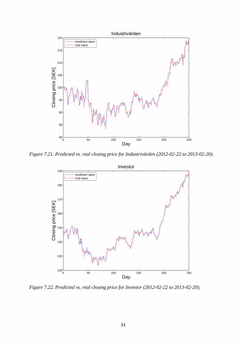
Figure 7.21. Predicted vs. real closing price for Industrivärden (2012-02-22 to 2013-02-20).
Figure 7.22. Predicted vs. real closing price for Investor (2012-02-22 to 2013-02-20).
0 50 100 150 200 25080
85
90
95
100
105
110
115
120
Industrivärden
Day
Clo
sin
g p
rice
[S
EK
]
predicted value
real value
0 50 100 150 200 250120
130
140
150
160
170
180
190
Investor
Day
Clo
sin
g p
rice
[S
EK
]
predicted value
real value
34
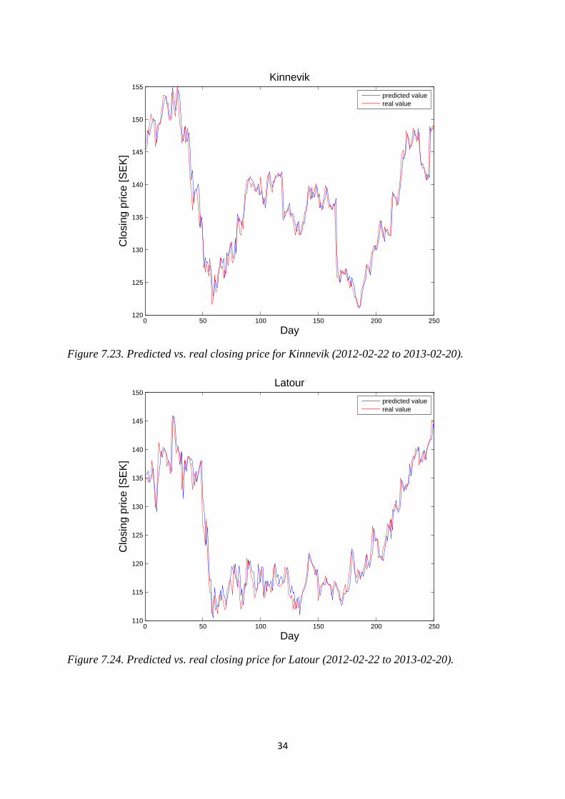
Figure 7.23. Predicted vs. real closing price for Kinnevik (2012-02-22 to 2013-02-20).
Figure 7.24. Predicted vs. real closing price for Latour (2012-02-22 to 2013-02-20).
0 50 100 150 200 250120
125
130
135
140
145
150
155
Kinnevik
Day
Clo
sin
g p
rice
[S
EK
]
predicted value
real value
0 50 100 150 200 250110
115
120
125
130
135
140
145
150
Latour
Day
Clo
sin
g p
rice
[S
EK
]
predicted value
real value

35
Figure 7.25. Predicted vs. real closing price for Lundbergföretagen
(2012-02-22 to 2013-02-20).
Figure 7.26. Predicted vs. real closing price for Meda (2012-02-22 to 2013-02-20).
0 50 100 150 200 250190
200
210
220
230
240
250
260
270
280
Lundbergföretagen
Day
Clo
sin
g p
rice
[S
EK
]
predicted value
real value
0 50 100 150 200 25060
62
64
66
68
70
72
74
76
78
Meda
Day
Clo
sin
g p
rice
[S
EK
]
predicted value
real value
36
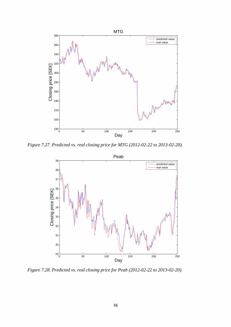
Figure 7.27. Predicted vs. real closing price for MTG (2012-02-22 to 2013-02-20).
Figure 7.28. Predicted vs. real closing price for Peab (2012-02-22 to 2013-02-20).
0 50 100 150 200 250180
200
220
240
260
280
300
320
340
360
380
MTG
Day
Clo
sin
g p
rice
[S
EK
]
predicted value
real value
0 50 100 150 200 25029
30
31
32
33
34
35
36
37
38
39
Peab
Day
Clo
sin
g p
rice
[S
EK
]
predicted value
real value
37
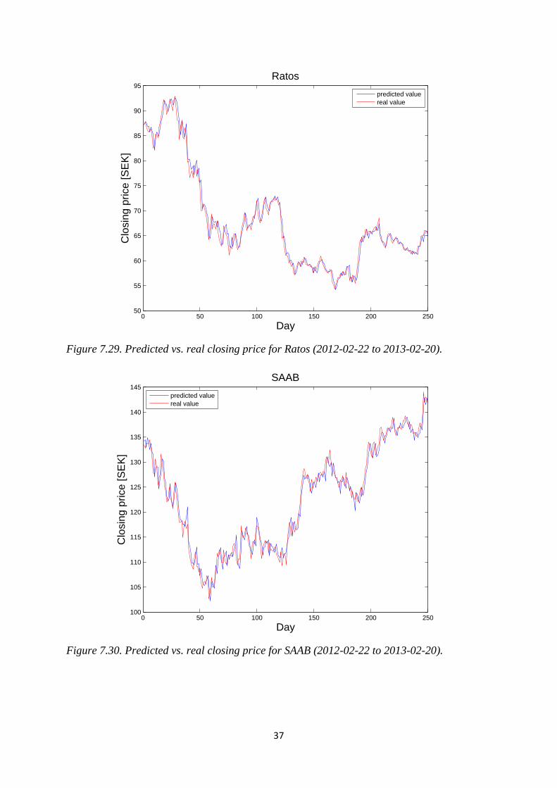
Figure 7.29. Predicted vs. real closing price for Ratos (2012-02-22 to 2013-02-20).
Figure 7.30. Predicted vs. real closing price for SAAB (2012-02-22 to 2013-02-20).
0 50 100 150 200 25050
55
60
65
70
75
80
85
90
95
Ratos
Day
Clo
sin
g p
rice
[S
EK
]
predicted value
real value
0 50 100 150 200 250100
105
110
115
120
125
130
135
140
145
SAAB
Day
Clo
sin
g p
rice
[S
EK
]
predicted value
real value
38
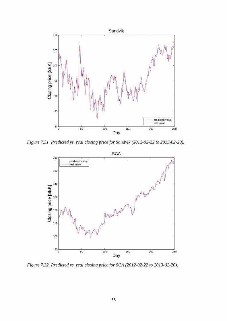
Figure 7.31. Predicted vs. real closing price for Sandvik (2012-02-22 to 2013-02-20).
Figure 7.32. Predicted vs. real closing price for SCA (2012-02-22 to 2013-02-20).
0 50 100 150 200 25080
85
90
95
100
105
110
Sandvik
Day
Clo
sin
g p
rice
[S
EK
]
predicted value
real value
0 50 100 150 200 25090
100
110
120
130
140
150
160
SCA
Day
Clo
sin
g p
rice
[S
EK
]
predicted value
real value
39
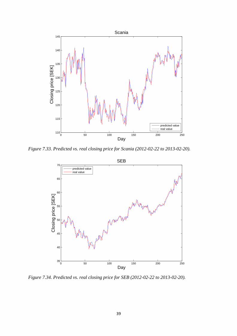
Figure 7.33. Predicted vs. real closing price for Scania (2012-02-22 to 2013-02-20).
Figure 7.34. Predicted vs. real closing price for SEB (2012-02-22 to 2013-02-20).
0 50 100 150 200 250110
115
120
125
130
135
140
145
Scania
Day
Clo
sin
g p
rice
[S
EK
]
predicted value
real value
0 50 100 150 200 25035
40
45
50
55
60
65
70
SEB
Day
Clo
sin
g p
rice
[S
EK
]
predicted value
real value
40
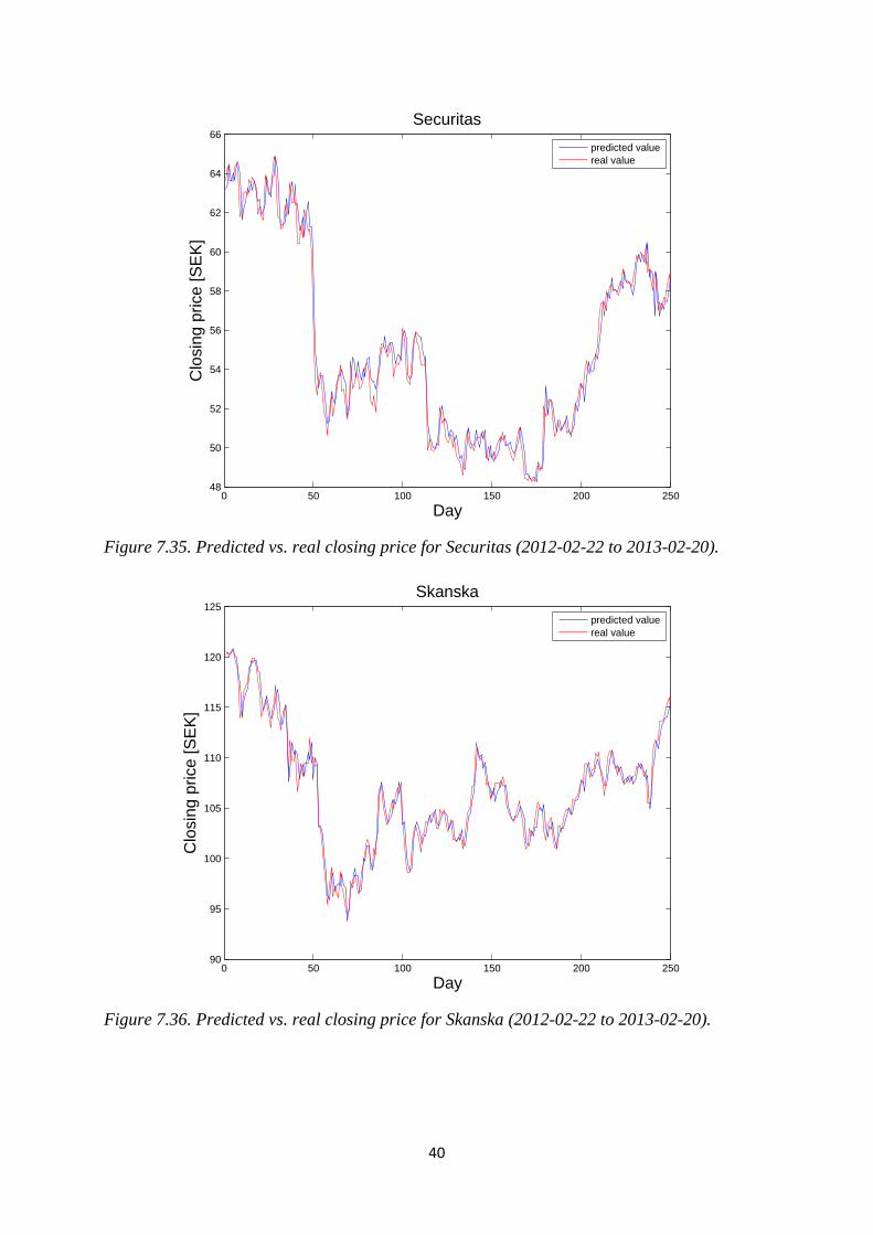
Figure 7.35. Predicted vs. real closing price for Securitas (2012-02-22 to 2013-02-20).
Figure 7.36. Predicted vs. real closing price for Skanska (2012-02-22 to 2013-02-20).
0 50 100 150 200 25048
50
52
54
56
58
60
62
64
66
Securitas
Day
Clo
sin
g p
rice
[S
EK
]
predicted value
real value
0 50 100 150 200 25090
95
100
105
110
115
120
125
Skanska
Day
Clo
sin
g p
rice
[S
EK
]
predicted value
real value

41
Figure 7.37. Predicted vs. real closing price for SKF (2012-02-22 to 2013-02-20).
Figure 7.38. Predicted vs. real closing price for SSAB (2012-02-22 to 2013-02-20).
0 50 100 150 200 250125
130
135
140
145
150
155
160
165
170
175
SKF
Day
Clo
sin
g p
rice
[S
EK
]
predicted value
real value
0 50 100 150 200 25045
50
55
60
65
70
75
SSAB
Day
Clo
sin
g p
rice
[S
EK
]
predicted value
real value
42
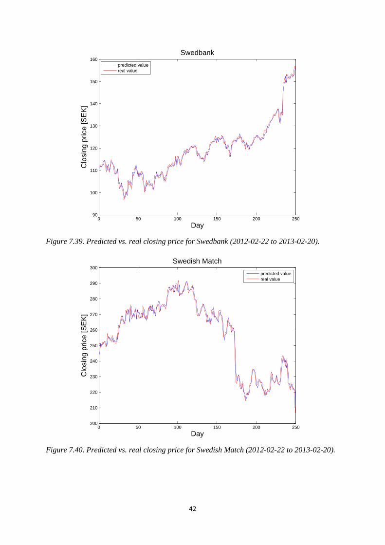
Figure 7.39. Predicted vs. real closing price for Swedbank (2012-02-22 to 2013-02-20).
Figure 7.40. Predicted vs. real closing price for Swedish Match (2012-02-22 to 2013-02-20).
0 50 100 150 200 25090
100
110
120
130
140
150
160
Swedbank
Day
Clo
sin
g p
rice
[S
EK
]
predicted value
real value
0 50 100 150 200 250200
210
220
230
240
250
260
270
280
290
300
Swedish Match
Day
Clo
sin
g p
rice
[S
EK
]
predicted value
real value
43
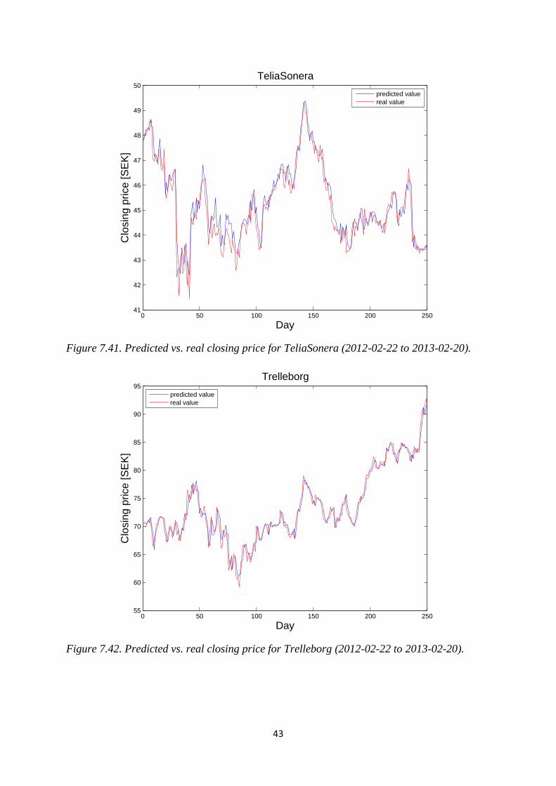
Figure 7.41. Predicted vs. real closing price for TeliaSonera (2012-02-22 to 2013-02-20).
Figure 7.42. Predicted vs. real closing price for Trelleborg (2012-02-22 to 2013-02-20).
0 50 100 150 200 25041
42
43
44
45
46
47
48
49
50
TeliaSonera
Day
Clo
sin
g p
rice
[S
EK
]
predicted value
real value
0 50 100 150 200 25055
60
65
70
75
80
85
90
95
Trelleborg
Day
Clo
sin
g p
rice
[S
EK
]
predicted value
real value
44
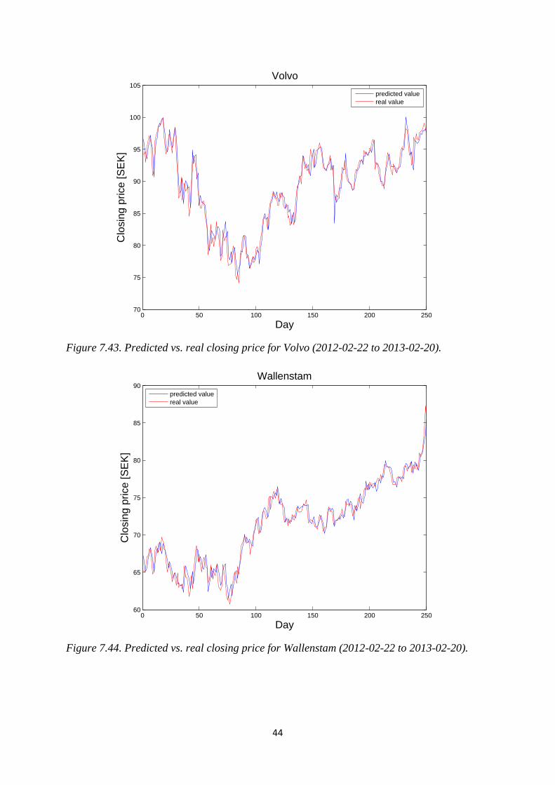
Figure 7.43. Predicted vs. real closing price for Volvo (2012-02-22 to 2013-02-20).
Figure 7.44. Predicted vs. real closing price for Wallenstam (2012-02-22 to 2013-02-20).
0 50 100 150 200 25070
75
80
85
90
95
100
105
Volvo
Day
Clo
sin
g p
rice
[S
EK
]
predicted value
real value
0 50 100 150 200 25060
65
70
75
80
85
90
Wallenstam
Day
Clo
sin
g p
rice
[S
EK
]
predicted value
real value

45
8.2 Yield using the model
Figure 7.45. Yield for Alfa Laval using the model (2012-02-22 to 2013-02-20).
Figure 7.46. Yield for Alliance Oil using the model (2012-02-22 to 2013-02-20).
46
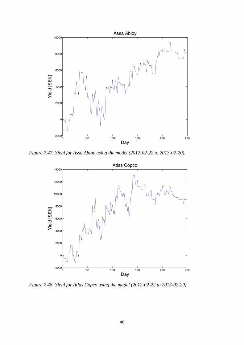
Figure 7.47. Yield for Assa Abloy using the model (2012-02-22 to 2013-02-20).
Figure 7.48. Yield for Atlas Copco using the model (2012-02-22 to 2013-02-20).

47
Figure 7.49. Yield for Axfood using the model (2012-02-22 to 2013-02-20).
Figure 7.50. Yield for Axis using the model (2012-02-22 to 2013-02-20).
48
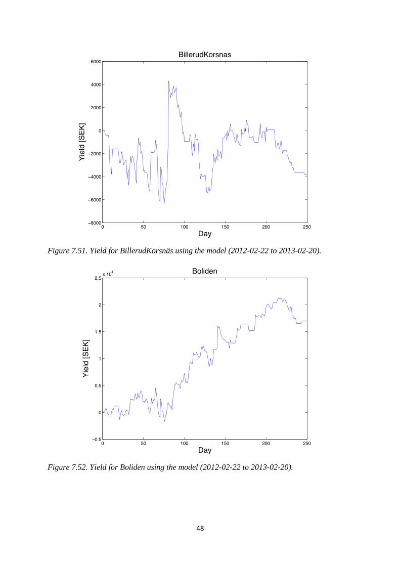
Figure 7.51. Yield for BillerudKorsnäs using the model (2012-02-22 to 2013-02-20).
Figure 7.52. Yield for Boliden using the model (2012-02-22 to 2013-02-20).
49
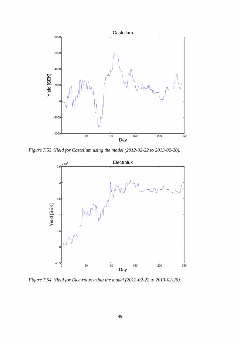
Figure 7.53. Yield for Castellum using the model (2012-02-22 to 2013-02-20).
Figure 7.54. Yield for Electrolux using the model (2012-02-22 to 2013-02-20).
50
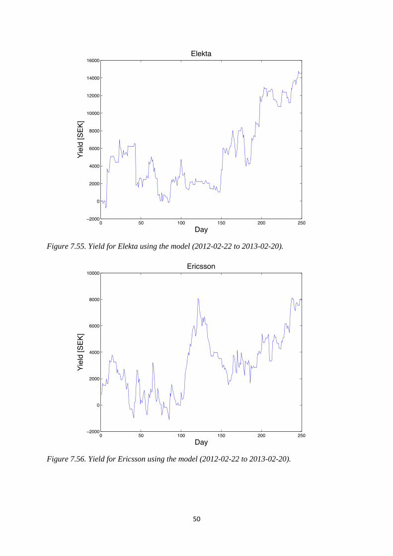
Figure 7.55. Yield for Elekta using the model (2012-02-22 to 2013-02-20).
Figure 7.56. Yield for Ericsson using the model (2012-02-22 to 2013-02-20).

51
Figure 7.57. Yield for Fabege using the model (2012-02-22 to 2013-02-20).
Figure 7.58. Yield for Getinge using the model (2012-02-22 to 2013-02-20).
52
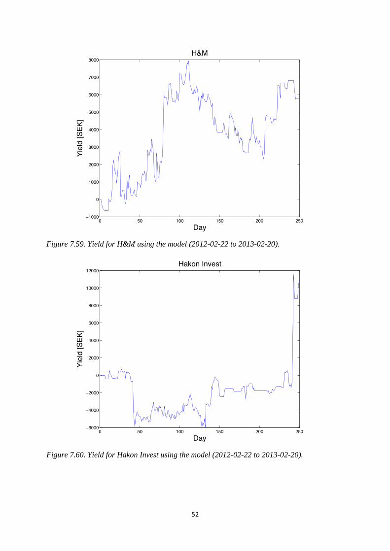
Figure 7.59. Yield for H&M using the model (2012-02-22 to 2013-02-20).
Figure 7.60. Yield for Hakon Invest using the model (2012-02-22 to 2013-02-20).

53
Figure 7.61. Yield for Hexagon using the model (2012-02-22 to 2013-02-20).
Figure 7.62. Yield for Holmen using the model (2012-02-22 to 2013-02-20).

54
Figure 7.63. Yield for Hufvudstaden using the model (2012-02-22 to 2013-02-20).
Figure 7.64. Yield for Husqvarna using the model (2012-02-22 to 2013-02-20).
55
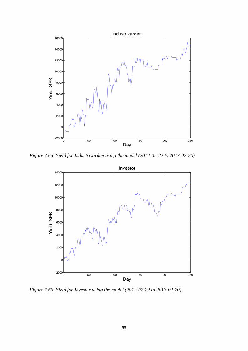
Figure 7.65. Yield for Industrivärden using the model (2012-02-22 to 2013-02-20).
Figure 7.66. Yield for Investor using the model (2012-02-22 to 2013-02-20).

56
Figure 7.67. Yield for Kinnevik using the model (2012-02-22 to 2013-02-20).
Figure 7.68. Yield for Latour using the model (2012-02-22 to 2013-02-20).

57
Figure 7.69. Yield for Lundbergföretagen using the model (2012-02-22 to 2013-02-20).
Figure 7.70. Yield for Meda using the model (2012-02-22 to 2013-02-20).

58
Figure 7.71. Yield for MTG using the model (2012-02-22 to 2013-02-20).
Figure 7.72. Yield for Peab using the model (2012-02-22 to 2013-02-20).
59
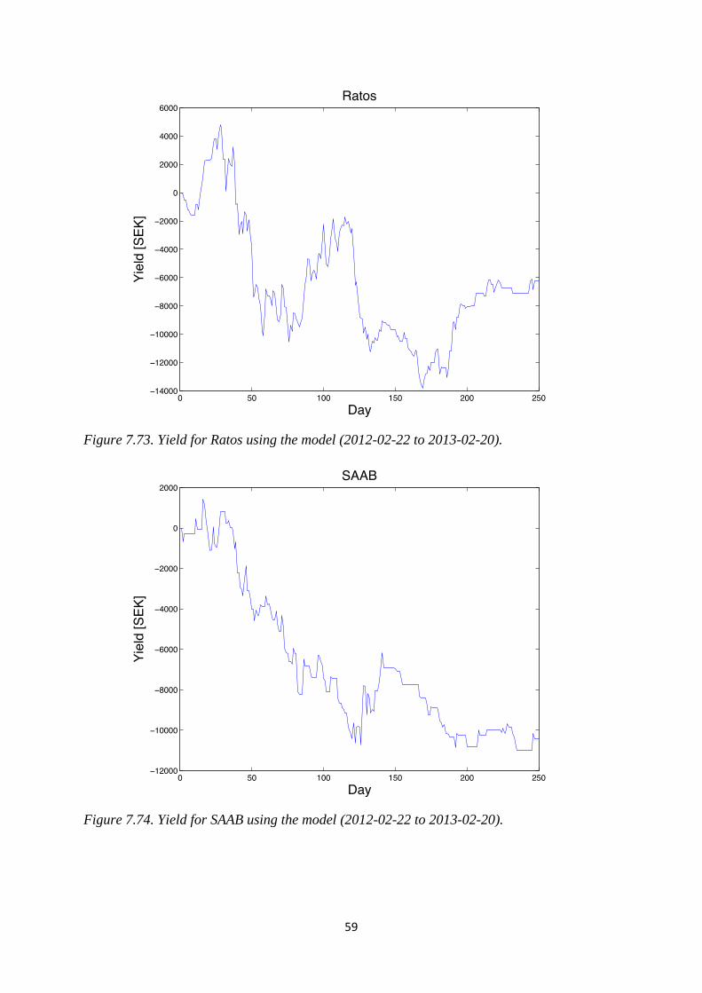
Figure 7.73. Yield for Ratos using the model (2012-02-22 to 2013-02-20).
Figure 7.74. Yield for SAAB using the model (2012-02-22 to 2013-02-20).
60
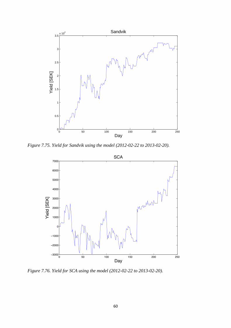
Figure 7.75. Yield for Sandvik using the model (2012-02-22 to 2013-02-20).
Figure 7.76. Yield for SCA using the model (2012-02-22 to 2013-02-20).
0 50 100 150 200 2500
0.5
1
1.5
2
2.5
3
3.5x 10
4 Sandvik
Day
Yie
ld [
SE
K]
61
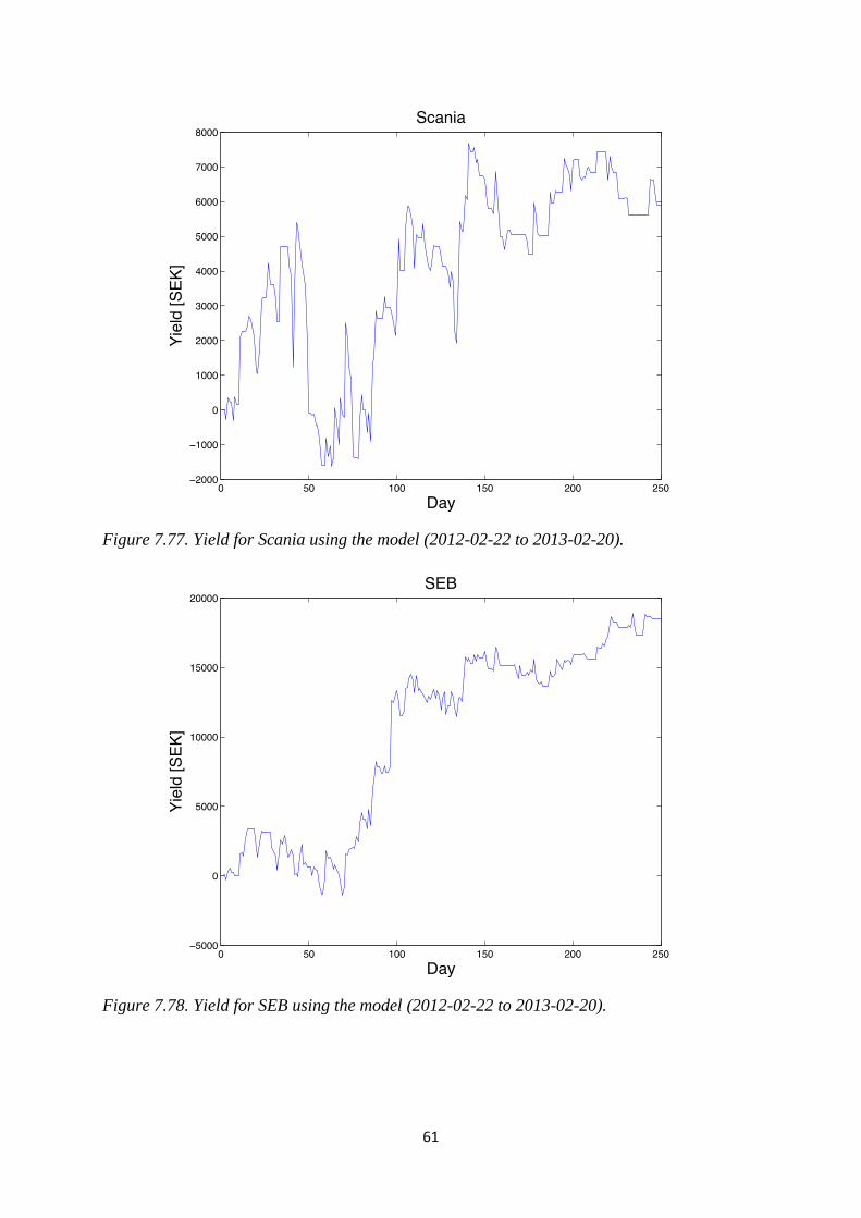
Figure 7.77. Yield for Scania using the model (2012-02-22 to 2013-02-20).
Figure 7.78. Yield for SEB using the model (2012-02-22 to 2013-02-20).

62
Figure 7.79. Yield for Securitas using the model (2012-02-22 to 2013-02-20).
Figure 7.80. Yield for Skanska using the model (2012-02-22 to 2013-02-20).

63
Figure 7.81. Yield for SKF using the model (2012-02-22 to 2013-02-20).
Figure 7.82. Yield for SSAB using the model (2012-02-22 to 2013-02-20).
0 50 100 150 200 2500
0.2
0.4
0.6
0.8
1
1.2
1.4
1.6
1.8
2x 10
4 SSAB
Day
Yie
ld [
SE
K]
64
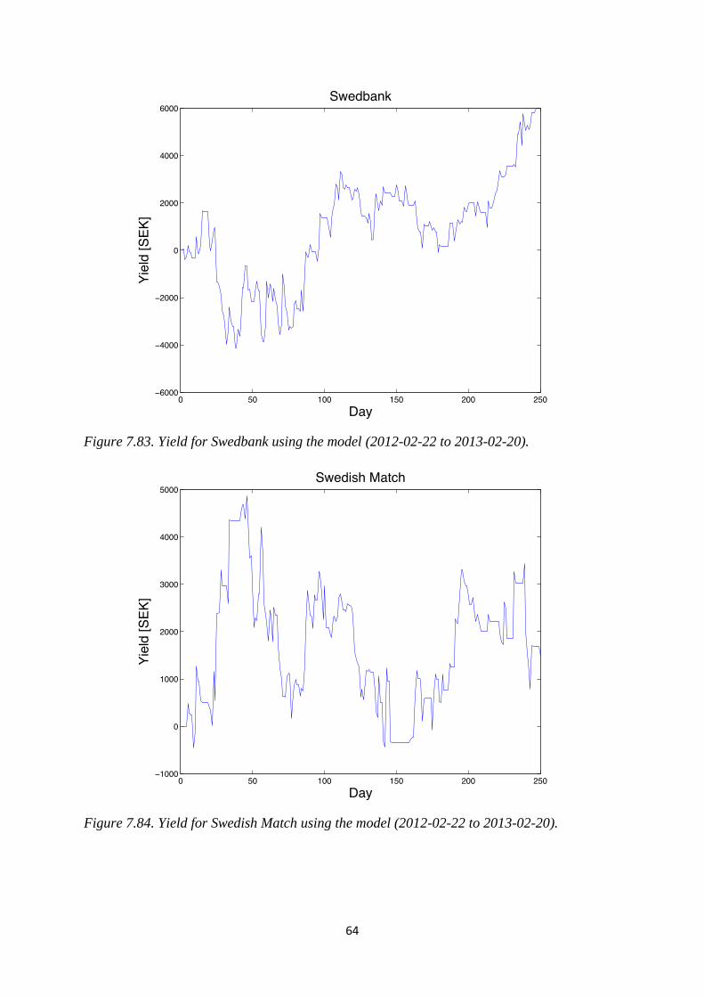
Figure 7.83. Yield for Swedbank using the model (2012-02-22 to 2013-02-20).
Figure 7.84. Yield for Swedish Match using the model (2012-02-22 to 2013-02-20).

65
Figure 7.85. Yield for TeliaSonera using the model (2012-02-22 to 2013-02-20).
Figure 7.86. Yield for Trelleborg using the model (2012-02-22 to 2013-02-20).

66
Figure 7.87. Yield for Volvo using the model (2012-02-22 to 2013-02-20).
Figure 7.88. Yield for Wallenstam using the model (2012-02-22 to 2013-02-20).

67
8.3 Stock exchange indexes
Figure 7.89. OMX Stockholm index (2008-01-02 to 2013-02-21).
Figure 7.90. Shanghai index (2008-01-02 to 2013-02-21).
0 200 400 600 800 1000 1200 1400500
600
700
800
900
1000
1100
1200
1300
OMX Stockholm
Day
Inde
x [
SE
K]
0 200 400 600 800 1000 1200 14001500
2000
2500
3000
3500
4000
4500
5000
Shanghai index
Inde
x [
SE
K]
Day
68
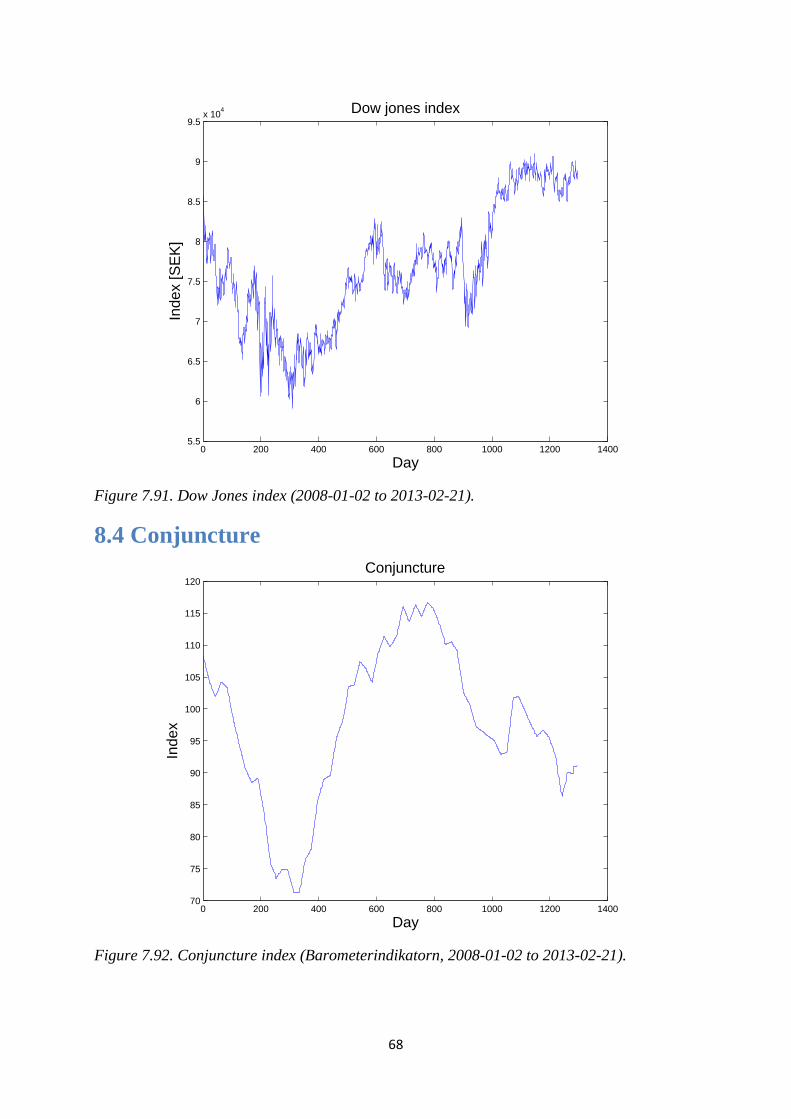
Figure 7.91. Dow Jones index (2008-01-02 to 2013-02-21).
8.4 Conjuncture
Figure 7.92. Conjuncture index (Barometerindikatorn, 2008-01-02 to 2013-02-21).
0 200 400 600 800 1000 1200 14005.5
6
6.5
7
7.5
8
8.5
9
9.5x 10
4 Dow jones index
Inde
x [
SE
K]
Day
0 200 400 600 800 1000 1200 140070
75
80
85
90
95
100
105
110
115
120
Day
Inde
x
Conjuncture
69
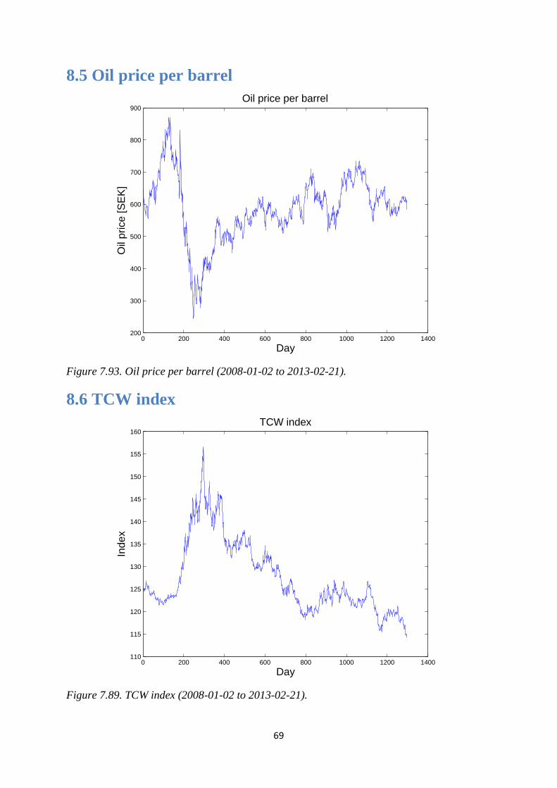
8.5 Oil price per barrel
Figure 7.93. Oil price per barrel (2008-01-02 to 2013-02-21).
8.6 TCW index
Figure 7.89. TCW index (2008-01-02 to 2013-02-21).
0 200 400 600 800 1000 1200 1400200
300
400
500
600
700
800
900
Oil price per barrel
Day
Oil
price [
SE
K]
0 200 400 600 800 1000 1200 1400110
115
120
125
130
135
140
145
150
155
160
TCW index
Inde
x
Day
70
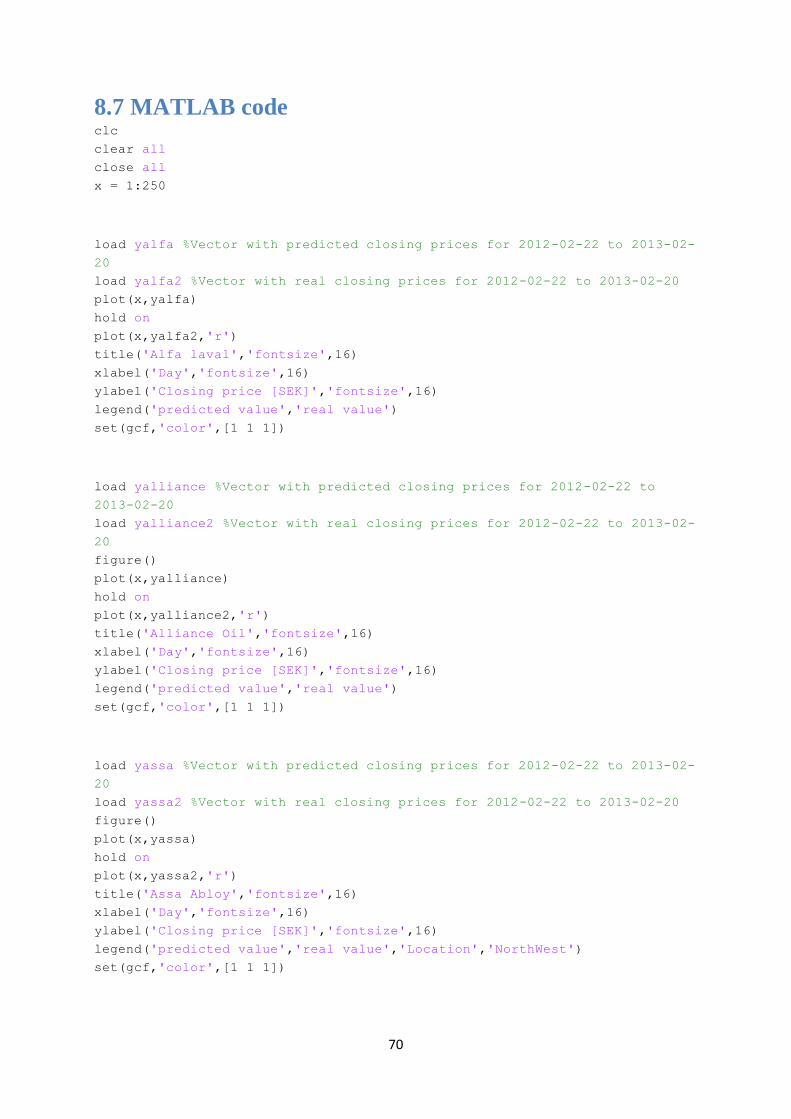
8.7 MATLAB code clc
clear all
close all
x = 1:250
load yalfa %Vector with predicted closing prices for 2012-02-22 to 2013-02-
20
load yalfa2 %Vector with real closing prices for 2012-02-22 to 2013-02-20
plot(x,yalfa)
hold on
plot(x,yalfa2,'r')
title('Alfa laval','fontsize',16)
xlabel('Day','fontsize',16)
ylabel('Closing price [SEK]','fontsize',16)
legend('predicted value','real value')
set(gcf,'color',[1 1 1])
load yalliance %Vector with predicted closing prices for 2012-02-22 to
2013-02-20
load yalliance2 %Vector with real closing prices for 2012-02-22 to 2013-02-
20
figure()
plot(x,yalliance)
hold on
plot(x,yalliance2,'r')
title('Alliance Oil','fontsize',16)
xlabel('Day','fontsize',16)
ylabel('Closing price [SEK]','fontsize',16)
legend('predicted value','real value')
set(gcf,'color',[1 1 1])
load yassa %Vector with predicted closing prices for 2012-02-22 to 2013-02-
20
load yassa2 %Vector with real closing prices for 2012-02-22 to 2013-02-20
figure()
plot(x,yassa)
hold on
plot(x,yassa2,'r')
title('Assa Abloy','fontsize',16)
xlabel('Day','fontsize',16)
ylabel('Closing price [SEK]','fontsize',16)
legend('predicted value','real value','Location','NorthWest')
set(gcf,'color',[1 1 1])
71
load yatlas %Vector with predicted closing prices for 2012-02-22 to 2013-
02-20
load yatlas2 %Vector with real closing prices for 2012-02-22 to 2013-02-20
figure()
plot(x,yatlas)
hold on
plot(x,yatlas2,'r')
title('Atlas Copco','fontsize',16)
xlabel('Day','fontsize',16)
ylabel('Closing price [SEK]','fontsize',16)
legend('predicted value','real value','Location','NorthWest')
set(gcf,'color',[1 1 1])
load yaxfood %Vector with predicted closing prices for 2012-02-22 to 2013-
02-20
load yaxfood2 %Vector with real closing prices for 2012-02-22 to 2013-02-20
figure()
plot(x,yaxfood)
hold on
plot(x,yaxfood2,'r')
title('Axfood','fontsize',16)
xlabel('Day','fontsize',16)
ylabel('Closing price [SEK]','fontsize',16)
legend('predicted value','real value','Location','NorthWest')
set(gcf,'color',[1 1 1])
load yaxis %Vector with predicted closing prices for 2012-02-22 to 2013-02-
20
load yaxis2 %Vector with real closing prices for 2012-02-22 to 2013-02-20
figure()
plot(x,yaxis)
hold on
plot(x,yaxis2,'r')
title('Axis','fontsize',16)
xlabel('Day','fontsize',16)
ylabel('Closing price [SEK]','fontsize',16)
legend('predicted value','real value')
set(gcf,'color',[1 1 1])
load ybillerud %Vector with predicted closing prices for 2012-02-22 to
2013-02-20
load ybillerud2 %Vector with real closing prices for 2012-02-22 to 2013-02-
20
figure()
plot(x,ybillerud)
hold on
plot(x,ybillerud2,'r')
title('BillerudKorsn‰s','fontsize',16)
xlabel('Day','fontsize',16)
72
ylabel('Closing price [SEK]','fontsize',16)
legend('predicted value','real value')
set(gcf,'color',[1 1 1])
load yboliden %Vector with predicted closing prices for 2012-02-22 to 2013-
02-20
load yboliden2 %Vector with real closing prices for 2012-02-22 to 2013-02-
20
figure()
plot(x,yboliden)
hold on
plot(x,yboliden2,'r')
title('Boliden','fontsize',16)
xlabel('Day','fontsize',16)
ylabel('Closing price [SEK]','fontsize',16)
legend('predicted value','real value','Location','NorthWest')
set(gcf,'color',[1 1 1])
load ycastellum %Vector with predicted closing prices for 2012-02-22 to
2013-02-20
load ycastellum2 %Vector with real closing prices for 2012-02-22 to 2013-
02-20
figure()
plot(x,ycastellum)
hold on
plot(x,ycastellum2,'r')
title('Castellum','fontsize',16)
xlabel('Day','fontsize',16)
ylabel('Closing price [SEK]','fontsize',16)
legend('predicted value','real value')
set(gcf,'color',[1 1 1])
load yelectro %Vector with predicted closing prices for 2012-02-22 to 2013-
02-20
load yelectro2 %Vector with real closing prices for 2012-02-22 to 2013-02-
20
figure()
plot(x,yelectro)
hold on
plot(x,yelectro2,'r')
title('Electrolux','fontsize',16)
xlabel('Day','fontsize',16)
ylabel('Closing price [SEK]','fontsize',16)
legend('predicted value','real value','Location','NorthWest')
set(gcf,'color',[1 1 1])
load yelekta %Vector with predicted closing prices for 2012-02-22 to 2013-
73
02-20
load yelekta2 %Vector with real closing prices for 2012-02-22 to 2013-02-20
figure()
plot(x,yelekta)
hold on
plot(x,yelekta2,'r')
title('Elekta','fontsize',16)
xlabel('Day','fontsize',16)
ylabel('Closing price [SEK]','fontsize',16)
legend('predicted value','real value')
set(gcf,'color',[1 1 1])
load yeric %Vector with predicted closing prices for 2012-02-22 to 2013-02-
20
load yeric2 %Vector with real closing prices for 2012-02-22 to 2013-02-20
figure()
plot(x,yeric)
hold on
plot(x,yeric2,'r')
title('Ericsson','fontsize',16)
xlabel('Day','fontsize',16)
ylabel('Closing price [SEK]','fontsize',16)
legend('predicted value','real value','Location','NorthWest')
set(gcf,'color',[1 1 1])
load yfabege %Vector with predicted closing prices for 2012-02-22 to 2013-
02-20
load yfabege2 %Vector with real closing prices for 2012-02-22 to 2013-02-20
figure()
plot(x,yfabege)
hold on
plot(x,yfabege2,'r')
title('Fabege','fontsize',16)
xlabel('Day','fontsize',16)
ylabel('Closing price [SEK]','fontsize',16)
legend('predicted value','real value','Location','NorthWest')
set(gcf,'color',[1 1 1])
load yget %Vector with predicted closing prices for 2012-02-22 to 2013-02-
20
load yget2 %Vector with real closing prices for 2012-02-22 to 2013-02-20
figure()
plot(x,yget)
hold on
plot(x,yget2,'r')
title('Getinge','fontsize',16)
xlabel('Day','fontsize',16)
ylabel('Closing price [SEK]','fontsize',16)
legend('predicted value','real value','Location','NorthWest')

74
set(gcf,'color',[1 1 1])
load yhakon %Vector with predicted closing prices for 2012-02-22 to 2013-
02-20
load yhakon2 %Vector with real closing prices for 2012-02-22 to 2013-02-20
figure()
plot(x,yhakon)
hold on
plot(x,yhakon2,'r')
title('Hakon Invest','fontsize',16)
xlabel('Day','fontsize',16)
ylabel('Closing price [SEK]','fontsize',16)
legend('predicted value','real value','Location','NorthWest')
set(gcf,'color',[1 1 1])
load yhex %Vector with predicted closing prices for 2012-02-22 to 2013-02-
20
load yhex2 %Vector with real closing prices for 2012-02-22 to 2013-02-20
figure()
plot(x,yhex)
hold on
plot(x,yhex2,'r')
title('Hexagon','fontsize',16)
xlabel('Day','fontsize',16)
ylabel('Closing price [SEK]','fontsize',16)
legend('predicted value','real value','Location','NorthWest')
set(gcf,'color',[1 1 1])
load yhm %Vector with predicted closing prices for 2012-02-22 to 2013-02-20
load yhm2 %Vector with real closing prices for 2012-02-22 to 2013-02-20
figure()
plot(x,yhm)
hold on
plot(x,yhm2,'r')
title('H&M','fontsize',16)
xlabel('Day','fontsize',16)
ylabel('Closing price [SEK]','fontsize',16)
legend('predicted value','real value')
set(gcf,'color',[1 1 1])
load yholm %Vector with predicted closing prices for 2012-02-22 to 2013-02-
20
load yholm2 %Vector with real closing prices for 2012-02-22 to 2013-02-20
figure()
plot(x,yholm)
hold on
plot(x,yholm2,'r')
title('Holmen','fontsize',16)
xlabel('Day','fontsize',16)
ylabel('Closing price [SEK]','fontsize',16)
75
legend('predicted value','real value','Location','SouthEast')
set(gcf,'color',[1 1 1])
load yhuf %Vector with predicted closing prices for 2012-02-22 to 2013-02-
20
load yhuf2 %Vector with real closing prices for 2012-02-22 to 2013-02-20
figure()
plot(x,yhuf)
hold on
plot(x,yhuf2,'r')
title('Hufvudstaden','fontsize',16)
xlabel('Day','fontsize',16)
ylabel('Closing price [SEK]','fontsize',16)
legend('predicted value','real value')
set(gcf,'color',[1 1 1])
load yhus %Vector with predicted closing prices for 2012-02-22 to 2013-02-
20
load yhus2 %Vector with real closing prices for 2012-02-22 to 2013-02-20
figure()
plot(x,yhus)
hold on
plot(x,yhus2,'r')
title('Husqvarna','fontsize',16)
xlabel('Day','fontsize',16)
ylabel('Closing price [SEK]','fontsize',16)
legend('predicted value','real value','Location','SouthEast')
set(gcf,'color',[1 1 1])
load yindu %Vector with predicted closing prices for 2012-02-22 to 2013-02-
20
load yindu2 %Vector with real closing prices for 2012-02-22 to 2013-02-20
figure()
plot(x,yindu)
hold on
plot(x,yindu2,'r')
title('Industriv‰rden','fontsize',16)
xlabel('Day','fontsize',16)
ylabel('Closing price [SEK]','fontsize',16)
legend('predicted value','real value','Location','NorthWest')
set(gcf,'color',[1 1 1])
load yinv %Vector with predicted closing prices for 2012-02-22 to 2013-02-
20
load yinv2 %Vector with real closing prices for 2012-02-22 to 2013-02-20
figure()
plot(x,yinv)
hold on
plot(x,yinv2,'r')
title('Investor','fontsize',16)

76
xlabel('Day','fontsize',16)
ylabel('Closing price [SEK]','fontsize',16)
legend('predicted value','real value','Location','NorthWest')
set(gcf,'color',[1 1 1])
load ykin %Vector with predicted closing prices for 2012-02-22 to 2013-02-
20
load ykin2 %Vector with real closing prices for 2012-02-22 to 2013-02-20
figure()
plot(x,ykin)
hold on
plot(x,ykin2,'r')
title('Kinnevik','fontsize',16)
xlabel('Day','fontsize',16)
ylabel('Closing price [SEK]','fontsize',16)
legend('predicted value','real value')
set(gcf,'color',[1 1 1])
load yla %Vector with predicted closing prices for 2012-02-22 to 2013-02-20
load yla2 %Vector with real closing prices for 2012-02-22 to 2013-02-20
figure()
plot(x,yla)
hold on
plot(x,yla2,'r')
title('Latour','fontsize',16)
xlabel('Day','fontsize',16)
ylabel('Closing price [SEK]','fontsize',16)
legend('predicted value','real value')
set(gcf,'color',[1 1 1])
load ylun %Vector with predicted closing prices for 2012-02-22 to 2013-02-
20
load ylun2 %Vector with real closing prices for 2012-02-22 to 2013-02-20
figure()
plot(x,ylun)
hold on
plot(x,ylun2,'r')
title('Lundbergfˆretagen','fontsize',16)
xlabel('Day','fontsize',16)
ylabel('Closing price [SEK]','fontsize',16)
legend('predicted value','real value','Location','NorthWest')
set(gcf,'color',[1 1 1])
load yme %Vector with predicted closing prices for 2012-02-22 to 2013-02-20
load yme2 %Vector with real closing prices for 2012-02-22 to 2013-02-20
figure()
plot(x,yme)
hold on
plot(x,yme2,'r')
title('Meda','fontsize',16)
77
xlabel('Day','fontsize',16)
ylabel('Closing price [SEK]','fontsize',16)
legend('predicted value','real value','Location','NorthWest')
set(gcf,'color',[1 1 1])
load ymtg %Vector with predicted closing prices for 2012-02-22 to 2013-02-
20
load ymtg2 %Vector with real closing prices for 2012-02-22 to 2013-02-20
figure()
plot(x,ymtg)
hold on
plot(x,ymtg2,'r')
title('MTG','fontsize',16)
xlabel('Day','fontsize',16)
ylabel('Closing price [SEK]','fontsize',16)
legend('predicted value','real value')
set(gcf,'color',[1 1 1])
load ype %Vector with predicted closing prices for 2012-02-22 to 2013-02-20
load ype2 %Vector with real closing prices for 2012-02-22 to 2013-02-20
figure()
plot(x,ype)
hold on
plot(x,ype2,'r')
title('Peab','fontsize',16)
xlabel('Day','fontsize',16)
ylabel('Closing price [SEK]','fontsize',16)
legend('predicted value','real value')
set(gcf,'color',[1 1 1])
load yra %Vector with predicted closing prices for 2012-02-22 to 2013-02-20
load yra2 %Vector with real closing prices for 2012-02-22 to 2013-02-20
figure()
plot(x,yra)
hold on
plot(x,yra2,'r')
title('Ratos','fontsize',16)
xlabel('Day','fontsize',16)
ylabel('Closing price [SEK]','fontsize',16)
legend('predicted value','real value')
set(gcf,'color',[1 1 1])
load ysaab %Vector with predicted closing prices for 2012-02-22 to 2013-02-
20
load ysaab2 %Vector with real closing prices for 2012-02-22 to 2013-02-20
figure()
plot(x,ysaab)
hold on
plot(x,ysaab2,'r')
title('SAAB','fontsize',16)
78
xlabel('Day','fontsize',16)
ylabel('Closing price [SEK]','fontsize',16)
legend('predicted value','real value','Location','NorthWest')
set(gcf,'color',[1 1 1])
load ysan %Vector with predicted closing prices for 2012-02-22 to 2013-02-
20
load ysan2 %Vector with real closing prices for 2012-02-22 to 2013-02-20
figure()
plot(x,ysan)
hold on
plot(x,ysan2,'r')
title('Sandvik','fontsize',16)
xlabel('Day','fontsize',16)
ylabel('Closing price [SEK]','fontsize',16)
legend('predicted value','real value','Location','SouthEast')
set(gcf,'color',[1 1 1])
load ysca %Vector with predicted closing prices for 2012-02-22 to 2013-02-
20
load ysca2 %Vector with real closing prices for 2012-02-22 to 2013-02-20
figure()
plot(x,ysca)
hold on
plot(x,ysca2,'r')
title('SCA','fontsize',16)
xlabel('Day','fontsize',16)
ylabel('Closing price [SEK]','fontsize',16)
legend('predicted value','real value','Location','NorthWest')
set(gcf,'color',[1 1 1])
load yscan %Vector with predicted closing prices for 2012-02-22 to 2013-02-
20
load yscan2 %Vector with real closing prices for 2012-02-22 to 2013-02-20
figure()
plot(x,yscan)
hold on
plot(x,yscan2,'r')
title('Scania','fontsize',16)
xlabel('Day','fontsize',16)
ylabel('Closing price [SEK]','fontsize',16)
legend('predicted value','real value','Location','SouthEast')
set(gcf,'color',[1 1 1])
load yseb %Vector with predicted closing prices for 2012-02-22 to 2013-02-
20
load yseb2 %Vector with real closing prices for 2012-02-22 to 2013-02-20
figure()
plot(x,yseb)
hold on
79
plot(x,yseb2,'r')
title('SEB','fontsize',16)
xlabel('Day','fontsize',16)
ylabel('Closing price [SEK]','fontsize',16)
legend('predicted value','real value','Location','NorthWest')
set(gcf,'color',[1 1 1])
load ysec %Vector with predicted closing prices for 2012-02-22 to 2013-02-
20
load ysec2 %Vector with real closing prices for 2012-02-22 to 2013-02-20
figure()
plot(x,ysec)
hold on
plot(x,ysec2,'r')
title('Securitas','fontsize',16)
xlabel('Day','fontsize',16)
ylabel('Closing price [SEK]','fontsize',16)
legend('predicted value','real value')
set(gcf,'color',[1 1 1])
load yskan %Vector with predicted closing prices for 2012-02-22 to 2013-02-
20
load yskan2 %Vector with real closing prices for 2012-02-22 to 2013-02-20
figure()
plot(x,yskan)
hold on
plot(x,yskan2,'r')
title('Skanska','fontsize',16)
xlabel('Day','fontsize',16)
ylabel('Closing price [SEK]','fontsize',16)
legend('predicted value','real value')
set(gcf,'color',[1 1 1])
load yskf %Vector with predicted closing prices for 2012-02-22 to 2013-02-
20
load yskf2 %Vector with real closing prices for 2012-02-22 to 2013-02-20
figure()
plot(x,yskf)
hold on
plot(x,yskf2,'r')
title('SKF','fontsize',16)
xlabel('Day','fontsize',16)
ylabel('Closing price [SEK]','fontsize',16)
legend('predicted value','real value')
set(gcf,'color',[1 1 1])
load yss %Vector with predicted closing prices for 2012-02-22 to 2013-02-20
load yss2 %Vector with real closing prices for 2012-02-22 to 2013-02-20
figure()
plot(x,yss)
80
hold on
plot(x,yss2,'r')
title('SSAB','fontsize',16)
xlabel('Day','fontsize',16)
ylabel('Closing price [SEK]','fontsize',16)
legend('predicted value','real value')
set(gcf,'color',[1 1 1])
load yswe %Vector with predicted closing prices for 2012-02-22 to 2013-02-
20
load yswe2 %Vector with real closing prices for 2012-02-22 to 2013-02-20
figure()
plot(x,yswe)
hold on
plot(x,yswe2,'r')
title('Swedbank','fontsize',16)
xlabel('Day','fontsize',16)
ylabel('Closing price [SEK]','fontsize',16)
legend('predicted value','real value','Location','NorthWest')
set(gcf,'color',[1 1 1])
load yswed %Vector with predicted closing prices for 2012-02-22 to 2013-02-
20
load yswed2 %Vector with real closing prices for 2012-02-22 to 2013-02-20
figure()
plot(x,yswed)
hold on
plot(x,yswed2,'r')
title('Swedish Match','fontsize',16)
xlabel('Day','fontsize',16)
ylabel('Closing price [SEK]','fontsize',16)
legend('predicted value','real value')
set(gcf,'color',[1 1 1])
load yte %Vector with predicted closing prices for 2012-02-22 to 2013-02-20
load yte2 %Vector with real closing prices for 2012-02-22 to 2013-02-20
figure()
plot(x,yte)
hold on
plot(x,yte2,'r')
title('TeliaSonera','fontsize',16)
xlabel('Day','fontsize',16)
ylabel('Closing price [SEK]','fontsize',16)
legend('predicted value','real value')
set(gcf,'color',[1 1 1])
load ytr %Vector with predicted closing prices for 2012-02-22 to 2013-02-20
load ytr2 %Vector with real closing prices for 2012-02-22 to 2013-02-20
figure()
plot(x,ytr)
81
hold on
plot(x,ytr2,'r')
title('Trelleborg','fontsize',16)
xlabel('Day','fontsize',16)
ylabel('Closing price [SEK]','fontsize',16)
legend('predicted value','real value','Location','NorthWest')
set(gcf,'color',[1 1 1])
load yv %Vector with predicted closing prices for 2012-02-22 to 2013-02-20
load yv2 %Vector with real closing prices for 2012-02-22 to 2013-02-20
figure()
plot(x,yv)
hold on
plot(x,yv2,'r')
title('Volvo','fontsize',16)
xlabel('Day','fontsize',16)
ylabel('Closing price [SEK]','fontsize',16)
legend('predicted value','real value')
set(gcf,'color',[1 1 1])
load yw %Vector with predicted closing prices for 2012-02-22 to 2013-02-20
load yw2 %Vector with real closing prices for 2012-02-22 to 2013-02-20
figure()
plot(x,yw)
hold on
plot(x,yw2,'r')
title('Wallenstam','fontsize',16)
xlabel('Day','fontsize',16)
ylabel('Closing price [SEK]','fontsize',16)
legend('predicted value','real value','Location','NorthWest')
set(gcf,'color',[1 1 1])
load yalfaavk %Vector with yield values for 2012-02-22 to 2013-02-20
figure()
plot(x,yalfaavk)
title('Alfa laval','fontsize',16)
xlabel('Day','fontsize',16)
ylabel('Yield [SEK]','fontsize',16)
set(gcf,'color',[1 1 1])
load yallavk %Vector with yield values for 2012-02-22 to 2013-02-20
figure()
plot(x,yallavk)
title('Alliance Oil','fontsize',16)
xlabel('Day','fontsize',16)
ylabel('Yield [SEK]','fontsize',16)
set(gcf,'color',[1 1 1])
load yassavk %Vector with yield values for 2012-02-22 to 2013-02-20
figure()
82
plot(x,yassavk)
title('Assa Abloy','fontsize',16)
xlabel('Day','fontsize',16)
ylabel('Yield [SEK]','fontsize',16)
set(gcf,'color',[1 1 1])
load yatavk %Vector with yield values for 2012-02-22 to 2013-02-20
figure()
plot(x,yatavk)
title('Atlas Copco','fontsize',16)
xlabel('Day','fontsize',16)
ylabel('Yield [SEK]','fontsize',16)
set(gcf,'color',[1 1 1])
load yaxfavk %Vector with yield values for 2012-02-22 to 2013-02-20
figure()
plot(x,yaxfavk)
title('Axfood','fontsize',16)
xlabel('Day','fontsize',16)
ylabel('Yield [SEK]','fontsize',16)
set(gcf,'color',[1 1 1])
load yaxavk %Vector with yield values for 2012-02-22 to 2013-02-20
figure()
plot(x,yaxavk)
title('Axis','fontsize',16)
xlabel('Day','fontsize',16)
ylabel('Yield [SEK]','fontsize',16)
set(gcf,'color',[1 1 1])
load ybilavk %Vector with yield values for 2012-02-22 to 2013-02-20
figure()
plot(x,ybilavk)
title('BillerudKorsn‰s','fontsize',16)
xlabel('Day','fontsize',16)
ylabel('Yield [SEK]','fontsize',16)
set(gcf,'color',[1 1 1])
load ybolavk %Vector with yield values for 2012-02-22 to 2013-02-20
figure()
plot(x,ybolavk)
title('Boliden','fontsize',16)
xlabel('Day','fontsize',16)
ylabel('Yield [SEK]','fontsize',16)
set(gcf,'color',[1 1 1])
load ycaavk %Vector with yield values for 2012-02-22 to 2013-02-20
figure()
plot(x,ycaavk)
title('Castellum','fontsize',16)
83
xlabel('Day','fontsize',16)
ylabel('Yield [SEK]','fontsize',16)
set(gcf,'color',[1 1 1])
load yelavk %Vector with yield values for 2012-02-22 to 2013-02-20
figure()
plot(x,yelavk)
title('Electrolux','fontsize',16)
xlabel('Day','fontsize',16)
ylabel('Yield [SEK]','fontsize',16)
set(gcf,'color',[1 1 1])
load yeleavk %Vector with yield values for 2012-02-22 to 2013-02-20
figure()
plot(x,yeleavk)
title('Elekta','fontsize',16)
xlabel('Day','fontsize',16)
ylabel('Yield [SEK]','fontsize',16)
set(gcf,'color',[1 1 1])
load yeravk %Vector with yield values for 2012-02-22 to 2013-02-20
figure()
plot(x,yeravk)
title('Ericsson','fontsize',16)
xlabel('Day','fontsize',16)
ylabel('Yield [SEK]','fontsize',16)
set(gcf,'color',[1 1 1])
load yfaavk %Vector with yield values for 2012-02-22 to 2013-02-20
figure()
plot(x,yfaavk)
title('Fabege','fontsize',16)
xlabel('Day','fontsize',16)
ylabel('Yield [SEK]','fontsize',16)
set(gcf,'color',[1 1 1])
load ygeavk %Vector with yield values for 2012-02-22 to 2013-02-20
figure()
plot(x,ygeavk)
title('Getinge','fontsize',16)
xlabel('Day','fontsize',16)
ylabel('Yield [SEK]','fontsize',16)
set(gcf,'color',[1 1 1])
load yhmavk %Vector with yield values for 2012-02-22 to 2013-02-20
figure()
plot(x,yhmavk)
title('H&M','fontsize',16)
xlabel('Day','fontsize',16)
ylabel('Yield [SEK]','fontsize',16)

84
set(gcf,'color',[1 1 1])
load yhakavk %Vector with yield values for 2012-02-22 to 2013-02-20
figure()
plot(x,yhakavk)
title('Hakon Invest','fontsize',16)
xlabel('Day','fontsize',16)
ylabel('Yield [SEK]','fontsize',16)
set(gcf,'color',[1 1 1])
break
load yhexavk %Vector with yield values for 2012-02-22 to 2013-02-20
figure()
plot(x,yhexavk)
title('Hexagon','fontsize',16)
xlabel('Day','fontsize',16)
ylabel('Yield [SEK]','fontsize',16)
set(gcf,'color',[1 1 1])
load yholavk %Vector with yield values for 2012-02-22 to 2013-02-20
figure()
plot(x,yholavk)
title('Holmen','fontsize',16)
xlabel('Day','fontsize',16)
ylabel('Yield [SEK]','fontsize',16)
set(gcf,'color',[1 1 1])
load yhufavk %Vector with yield values for 2012-02-22 to 2013-02-20
figure()
plot(x,yhufavk)
title('Hufvudstaden','fontsize',16)
xlabel('Day','fontsize',16)
ylabel('Yield [SEK]','fontsize',16)
set(gcf,'color',[1 1 1])
load yhusavk %Vector with yield values for 2012-02-22 to 2013-02-20
figure()
plot(x,yhusavk)
title('Husqvarna','fontsize',16)
xlabel('Day','fontsize',16)
ylabel('Yield [SEK]','fontsize',16)
set(gcf,'color',[1 1 1])
load yindavk %Vector with yield values for 2012-02-22 to 2013-02-20
figure()
plot(x,yindavk)
title('Industriv‰rden','fontsize',16)
xlabel('Day','fontsize',16)
ylabel('Yield [SEK]','fontsize',16)
set(gcf,'color',[1 1 1])
85
load yinvavk %Vector with yield values for 2012-02-22 to 2013-02-20
figure()
plot(x,yinvavk)
title('Investor','fontsize',16)
xlabel('Day','fontsize',16)
ylabel('Yield [SEK]','fontsize',16)
set(gcf,'color',[1 1 1])
load ykinavk %Vector with yield values for 2012-02-22 to 2013-02-20
figure()
plot(x,ykinavk)
title('Kinnevik','fontsize',16)
xlabel('Day','fontsize',16)
ylabel('Yield [SEK]','fontsize',16)
set(gcf,'color',[1 1 1])
load ylaavk %Vector with yield values for 2012-02-22 to 2013-02-20
figure()
plot(x,ylaavk)
title('Latour','fontsize',16)
xlabel('Day','fontsize',16)
ylabel('Yield [SEK]','fontsize',16)
set(gcf,'color',[1 1 1])
load ylundavk %Vector with yield values for 2012-02-22 to 2013-02-20
figure()
plot(x,ylundavk)
title('Lundbergfˆretagen','fontsize',16)
xlabel('Day','fontsize',16)
ylabel('Yield [SEK]','fontsize',16)
set(gcf,'color',[1 1 1])
load ymedavk %Vector with yield values for 2012-02-22 to 2013-02-20
figure()
plot(x,ymedavk)
title('Meda','fontsize',16)
xlabel('Day','fontsize',16)
ylabel('Yield [SEK]','fontsize',16)
set(gcf,'color',[1 1 1])
load ymtgavk %Vector with yield values for 2012-02-22 to 2013-02-20
figure()
plot(x,ymtgavk)
title('MTG','fontsize',16)
xlabel('Day','fontsize',16)
ylabel('Yield [SEK]','fontsize',16)
set(gcf,'color',[1 1 1])
load ypavk %Vector with yield values for 2012-02-22 to 2013-02-20
figure()
86
plot(x,ypavk)
title('Peab','fontsize',16)
xlabel('Day','fontsize',16)
ylabel('Yield [SEK]','fontsize',16)
set(gcf,'color',[1 1 1])
load yraavk %Vector with yield values for 2012-02-22 to 2013-02-20
figure()
plot(x,yraavk)
title('Ratos','fontsize',16)
xlabel('Day','fontsize',16)
ylabel('Yield [SEK]','fontsize',16)
set(gcf,'color',[1 1 1])
load ysaavk %Vector with yield values for 2012-02-22 to 2013-02-20
figure()
plot(x,ysaavk)
title('SAAB','fontsize',16)
xlabel('Day','fontsize',16)
ylabel('Yield [SEK]','fontsize',16)
set(gcf,'color',[1 1 1])
load ysandavk %Vector with yield values for 2012-02-22 to 2013-02-20
figure()
plot(x,ysandavk)
title('Sandvik','fontsize',16)
xlabel('Day','fontsize',16)
ylabel('Yield [SEK]','fontsize',16)
set(gcf,'color',[1 1 1])
load yscaavk %Vector with yield values for 2012-02-22 to 2013-02-20
figure()
plot(x,yscaavk)
title('SCA','fontsize',16)
xlabel('Day','fontsize',16)
ylabel('Yield [SEK]','fontsize',16)
set(gcf,'color',[1 1 1])
load yscanavk %Vector with yield values for 2012-02-22 to 2013-02-20
figure()
plot(x,yscanavk)
title('Scania','fontsize',16)
xlabel('Day','fontsize',16)
ylabel('Yield [SEK]','fontsize',16)
set(gcf,'color',[1 1 1])
load ysebavk %Vector with yield values for 2012-02-22 to 2013-02-20
figure()
plot(x,ysebavk)
title('SEB','fontsize',16)

87
xlabel('Day','fontsize',16)
ylabel('Yield [SEK]','fontsize',16)
set(gcf,'color',[1 1 1])
load ysecavk %Vector with yield values for 2012-02-22 to 2013-02-20
figure()
plot(x,ysecavk)
title('Securitas','fontsize',16)
xlabel('Day','fontsize',16)
ylabel('Yield [SEK]','fontsize',16)
set(gcf,'color',[1 1 1])
load yskaavk %Vector with yield values for 2012-02-22 to 2013-02-20
figure()
plot(x,yskaavk)
title('Skanska','fontsize',16)
xlabel('Day','fontsize',16)
ylabel('Yield [SEK]','fontsize',16)
set(gcf,'color',[1 1 1])
load yskfavk %Vector with yield values for 2012-02-22 to 2013-02-20
figure()
plot(x,yskfavk)
title('SKF','fontsize',16)
xlabel('Day','fontsize',16)
ylabel('Yield [SEK]','fontsize',16)
set(gcf,'color',[1 1 1])
load yssavk %Vector with yield values for 2012-02-22 to 2013-02-20
figure()
plot(x,yssavk)
title('SSAB','fontsize',16)
xlabel('Day','fontsize',16)
ylabel('Yield [SEK]','fontsize',16)
set(gcf,'color',[1 1 1])
load ysweavk %Vector with yield values for 2012-02-22 to 2013-02-20
figure()
plot(x,ysweavk)
title('Swedbank','fontsize',16)
xlabel('Day','fontsize',16)
ylabel('Yield [SEK]','fontsize',16)
set(gcf,'color',[1 1 1])
load yswedavk %Vector with yield values for 2012-02-22 to 2013-02-20
figure()
plot(x,yswedavk)
title('Swedish Match','fontsize',16)
xlabel('Day','fontsize',16)
ylabel('Yield [SEK]','fontsize',16)
88
set(gcf,'color',[1 1 1])
load yteavk %Vector with yield values for 2012-02-22 to 2013-02-20
figure()
plot(x,yteavk)
title('TeliaSonera','fontsize',16)
xlabel('Day','fontsize',16)
ylabel('Yield [SEK]','fontsize',16)
set(gcf,'color',[1 1 1])
load ytravk %Vector with yield values for 2012-02-22 to 2013-02-20
figure()
plot(x,ytravk)
title('Trelleborg','fontsize',16)
xlabel('Day','fontsize',16)
ylabel('Yield [SEK]','fontsize',16)
set(gcf,'color',[1 1 1])
load yvoavk %Vector with yield values for 2012-02-22 to 2013-02-20
figure()
plot(x,yvoavk)
title('Volvo','fontsize',16)
xlabel('Day','fontsize',16)
ylabel('Yield [SEK]','fontsize',16)
set(gcf,'color',[1 1 1])
load ywaavk %Vector with yield values for 2012-02-22 to 2013-02-20
figure()
plot(x,ywaavk)
title('Wallenstam','fontsize',16)
xlabel('Day','fontsize',16)
ylabel('Yield [SEK]','fontsize',16)
set(gcf,'color',[1 1 1])
load ytotavk %Vector with total yield values for 2012-02-22 to 2013-02-20
figure()
plot(x,ytotavk)
title('Total Yield','fontsize',16)
xlabel('Day','fontsize',16)
ylabel('Yield [SEK]','fontsize',16)
set(gcf,'color',[1 1 1])
x = 1:1296;
load omx %Vector with OMX index for 2008-01-02 to 2013-02-20
figure()
plot(x,omx)
title('OMX Stockholm','fontsize',16)
xlabel('Day','fontsize',16)
ylabel('Index [SEK]','fontsize',16)
set(gcf,'color',[1 1 1])
89
load kon %Vector with conjuncture values for 2008-01-02 to 2013-02-20
figure()
plot(x,baro)
xlabel('Day','fontsize',16)
ylabel('Index','fontsize',16)
title('Conjuncture','fontsize',16)
set(gcf,'color',[1 1 1])
load oil %Vector with oil price per barrel for 2008-01-02 to 2013-02-20
figure()
plot(x,olja)
title('Oil price per barrel','fontsize',16)
xlabel('Day','fontsize',16)
ylabel('Oil price [SEK]','fontsize',16)
set(gcf,'color',[1 1 1])
load dow %Vector with dow jones index for 2008-01-02 to 2013-02-20
figure()
plot(x,dow)
title('Dow jones index','fontsize',16)
ylabel('Index [SEK]','fontsize',16)
xlabel('Day','fontsize',16)
set(gcf,'color',[1 1 1])
load shang %Vector with shanghai index for 2008-01-02 to 2013-02-20
figure()
plot(x,shang)
title('Shanghai index','fontsize',16)
ylabel('Index [SEK]','fontsize',16)
xlabel('Day','fontsize',16)
set(gcf,'color',[1 1 1])
load tcw %Vector with TCW index for 2008-01-02 to 2013-02-20
figure()
plot(x,tcw)
title('TCW index','fontsize',16)
ylabel('Index','fontsize',16)
xlabel('Day','fontsize',16)
set(gcf,'color',[1 1 1])
%Plot for regression channel
clc
clear all
close all
load y % Vector with closing prices 2008-01-02 to 2013-02-21
x=[1:1296]';
c=regress(x(400:500),y(400:500));
90
a=y(400);
b=x(400);
j=400:500;
k=(y(500)-y(400))/length(j);
m=y(400)-k*400;
for i=400:1000
d(i)=k*x(i)+m;
end
d=d(400:1000)';
m1=m+12.5;
for i=400:1000
e(i)=k*x(i)+m1;
end
e=e(400:1000)';
m2=m-12.5;
for i=400:1000
f(i)=k*x(i)+m2;
end
f=f(400:1000)';
plot(x,y);
hold on
plot(b,a,'r*');
hold on
plot(x(400:1000),d,'black');
hold on
plot(x(400:1000),e,'black');
hold on
plot(x(400:1000),f,'black');
hold on
plot(x(500),y(500),'r*')
hold on
plot(579.0295,81.9941,'ro')
ylabel('Closing price [SEK]','fontsize', 16)
xlabel('Days','fontsize', 16)
title('VOLVO AB, B share','fontsize', 16)
91
Chapter 9 References
9.1 References
[1] http://www.nasdaqomxnordic.com/aktier/historiskakurser/
[2] http://www.nasdaqomxnordic.com/nyheter/foretagsmeddelanden/
[3] http://www.di.se/stockwatch/
[4] http://www.ekonomifakta.se/sv/Fakta/Ekonomi/Finansiell-
utveckling/Vaxelkursutvecklingen-TCW-index/
[5] http://www.fi.se/Register/Insynsregistret/
[6] http://www.ekonomifakta.se/sv/Fakta/Ekonomi/Tillvaxt/Konjunkturen---
Barometerindikatorn/
[7] http://www.riksbank.se/sv/Rantor-och-valutakurser/Reporantan-tabell/
[8] https://research.stlouisfed.org/fred2/series/DJIA/downloaddata?cid=32255
[9] http://finance.yahoo.com/q/hp?s=000001.SS&a=00&b=2&c=2008&d=01&e=21&f
=2013&g=d
[10] http://www.eia.gov/dnav/pet/pet_pri_spt_s1_d.htm
[11] http://www.oanda.com/lang/sv/currency/historical-rates/
[12] http://user.tninet.se/~sjx942j/modell/Regressionskanalvecka.htm
[13] http://www.aktiespararna.se/ungaaktiesparare/Utbildning/Aktier/Aktiekursen/
[14] http://www.youtube.com/watch?v=Wj9_usXqErk
[15] http://www.ssc.wisc.edu/~bhansen/econometrics/Econometrics.pdf
[16] Harald Lang, Topics on Applied Mathematical Statistics, July 2012, version 0.93
[17] MATLAB R2012, calculation software created by: 1994-2012 The MathWorks Inc.
[18] Microsoft Excel 2010, Spreadsheet software created by: 1975-2012 Microsoft
Corporation

92
[19] Minitab 16, Statistics package created by: 1972-2012 Barbara F. Ryan, Thomas A. Ryan,
Jr., and Brian L. Joiner
[20] http://www-stat.stanford.edu/~jtaylo/courses/stats203/notes/selection.pdf


