PREDICTING OVER TARGET BASELINE (OTB)

ACQUISITION CONTRACTS

THESIS

Kristine E. Thickstun, Captain, USAF

AFIT/GCA/ENC/10-01

DEPARTMENT OF THE AIR FORCE AIR UNIVERSITY

AIR FORCE INSTITUTE OF TECHNOLOGY

Wright-Patterson Air Force Base, Ohio

APPROVED FOR PUBLIC RELEASE; DISTRIBUTION UNLIMITED

The views expressed in this thesis are those of the author and do not reflect the official policy or position of the United States Air Force, Department of Defense, or the United States Government.

AFIT/GCA/ENC/10-01

PREDICTING OVER TARGET BASELINE (OTB) ACQUISITION CONTRACTS

THESIS

Presented to the Faculty

Department of Mathematics and Statistics

Graduate School of Engineering and Management

Air Force Institute of Technology

Air University

Air Education and Training Command

In Partial Fulfillment of the Requirements for the

Degree of Master of Science in Cost Analysis

Kristine E. Thickstun, BS, MBA

Captain, USAF

March 2010

APPROVED FOR PUBLIC RELEASE; DISTRIBUTION UNLIMITED.

AFIT/GCA/ENC/10-01

PREDICTING OVER TARGET BASELINE (OTB) ACQUISITION CONTRACTS

Kristine E. Thickstun, BS, MBA

Captain, USAF

Approved: _______//signed//_______________________ _March 2010_____ Dr. Edward D. White (Chairman) Date _______//signed//_______________________ _March 2010_____ Lt Col Eric J. Unger, PhD (Member) Date _______//signed//_______________________ _March 2010_____ Capt Elizabeth T. Poulos, MBA, MS (Member) Date

iv

AFIT/GCA/ENC/10-01

Abstract

Cost estimators use a variety of methods to develop estimates at completion

(EACs) and new methods continue to be developed. Research has shown there is no best

method for computing EACs for all acquisition contracts. However, some methods

perform better under specific circumstances. In 2009, Captain Trahan investigated the

use of a Gompertz growth model for developing EACs. She found that this method is

more reliable for Over Target Baseline (OTB) contracts than the standard indexed based

approaches. Captain Trahan’s model is an excellent model to use for OTB contracts or

contracts with a high likelihood of becoming an OTB contract. In this study, we attempt

to develop a model that predicts whether an acquisition contract is likely to become an

OTB. By identifying contracts that are likely to become OTB, we can apply the

Gompertz growth model to develop better EACs. Furthermore, an OTB, by definition,

recognizes a cost overrun. Therefore, the ability to predict OTBs would allow us to

understand what may cause cost overruns. However, our models indicate that we are

unable to predict an OTB. This indicates that the OTB process may be used randomly

which leads us to question the benefits of OTBs.

v

Acknowledgements

I would like to thank my family for all of their support during my time at AFIT.

They were always there for me and motivated me throughout the thesis process. I would

especially like to thank my husband. I could not have done this without the

encouragement that he has given me.

I would also like to thank my thesis committee for all of their help. Dr. White

provided me with very helpful guidance and motivation throughout the process. He

helped me obtain a better understanding of the statistical processes and the different ways

we can approach our problem. Lt Col Unger also helped me address issues associated

with dealing with the earned value databases.

Finally, I would like to thank all of the support help at DAMIR who helped me

understand the SARs and DAES databases.

Kristine Thickstun

vi

Table of Contents

Abstract .............................................................................................................................. iv  Acknowledgements ............................................................................................................. v  Table of Contents ............................................................................................................... vi  List of Figures .................................................................................................................. viii  List of Tables ..................................................................................................................... ix  I: Introduction ..................................................................................................................... 1 

Background ..................................................................................................................... 1 Purpose of this Study ...................................................................................................... 3 Study Process .................................................................................................................. 5 

II: Literature Review ........................................................................................................... 6 

Introduction ..................................................................................................................... 6 Earned Value Management (EVM) ................................................................................ 6 Developing Estimates at Completion (EACs) ................................................................ 9 

Developing EACs Using a Growth Model ............................................................... 11 Cost Overruns and the OTB Process ............................................................................ 14 Identifying an OTB in Practice ..................................................................................... 18 

Cost Overruns vs. Cost Growth ................................................................................ 19 Logistic Regression Two-Step Models ......................................................................... 20 Summary ....................................................................................................................... 22 

III: Data and Methodology................................................................................................ 23 

Introduction ................................................................................................................... 23 Data Sources ................................................................................................................. 23 Data Normalization ....................................................................................................... 26 

Inflation ..................................................................................................................... 27 Combining DAES and SARs Datasets ..................................................................... 28 Management Reserve (MR) Missing Values ............................................................ 28 

Data Assumptions and Limitations ............................................................................... 29 The Response Variable: Over Target Baseline ............................................................ 30 Predictor Variables ........................................................................................................ 31 Logistic Regression Models .......................................................................................... 32 Interpreting the Predictors for the Logistic Regression Model ..................................... 35 

Page

vii

Assessing the Predictive Ability of the Model ............................................................. 36 Summary ....................................................................................................................... 38 

IV: Results and Analysis ................................................................................................... 39 

Introduction ................................................................................................................... 39 Distinguishing Between Production and Development Contracts ................................ 39 Approach to Developing Models .................................................................................. 40 Logistic Regression Models for Development (RDT&E) Contracts ............................ 41 Logistic Regression Models for Production (Procurement) Contracts ......................... 44 Validation of Logistic Regression Models ................................................................... 46 Additional Attempts at Predicting OTBs ...................................................................... 49 Conclusion .................................................................................................................... 50 

V: Discussion and Conclusion .......................................................................................... 51 

Thesis Purpose .............................................................................................................. 51 Summary of Results ...................................................................................................... 51 Policy Implications ....................................................................................................... 52 Future Research ............................................................................................................ 53 

Appendix A: The Office of the Under Secretary of Defense (OUSD) (Comptroller) Raw Inflation Indices ................................................................................................................ 55  Appendix B: The Office of the Under Secretary of Defense OUSD (Comptroller) Outlay Rates .................................................................................................................................. 56  Appendix C: Weighted Inflation Indices ......................................................................... 57  Appendix D: Logistic Regression Models: Development Contracts ............................... 58  Appendix E: Logistic Regression Models: Production Contracts ................................... 60  Bibliography ..................................................................................................................... 62  Vita .................................................................................................................................... 64 

viii

List of Figures Page

Figure 1: Performance Measurement Baseline (Christensen, 1999) ................................. 8  Figure 2: Development Growth Model (Trahan, 2009) ................................................... 12  Figure 3: The OTB Process Flow (DAU, 2003) .............................................................. 16  Figure 4: EVM Contractual Price Components (DAU, 2009) ......................................... 19  Figure 5: Plot of Binary Data ............................................................................................ 33  Figure 6: Box Plot of % Complete Prior to OTB............................................................. 49 

ix

List of Tables Page

Table 1: EVM Performance Indices .................................................................................. 9  Table 2: EAC Formula Using Growth Model (Trahan, 2009)......................................... 12  Table 3: MAPE Comparison (Trahan, 2009) ................................................................... 13  Table 4: Final Dataset Used in Analysis ........................................................................... 30  Table 5: Logistic Regression Equation, Single Variable Model ....................................... 34  Table 6: Logistic Regression Equation, Multivariate Model ............................................ 34  Table 7: Interpreting the Area Under the ROC Curve (Hosmer and Lemeshow, 2000) .. 37  Table 8: Development Model Parameters ........................................................................ 44  Table 9: Production Model Parameters............................................................................. 46  Table 10: Computational Form of Logistic Regression Equation .................................... 47  Table 11: Model Validation Results ................................................................................. 48 

1

PREDICTING OVER TARGET BASELINE (OTB) ACQUISITION CONTRACTS

I: Introduction

Background Approximately twenty percent of all acquisition contracts in the DoD experienced

cost overruns over the past 20 years (based on analysis dataset). An Over Target

Baseline (OTB) formally recognizes these cost overruns. By examining eighty percent of

contracts between 1990 and 2005 for Major Defense Acquisition Programs (MDAPs), we

identify over $26 billion in cost overruns (BY09$). The average cost overrun for each

contract experiencing an OTB is $321 million (BY09$).

Since cost overruns are a major concern for the entire Department of Defense, it is

important to understand why they occur. Two potential reasons for cost overruns are: 1)

The existing cost estimates are not accurate to begin with which leads to the actual costs

being far from the estimate and 2) Program costs are not effectively controlled to prevent

overruns. Solutions to these problems include improving the original cost estimates,

improving our control mechanisms for acquisition programs, and managing factors that

lead to cost overruns. The DoD uses the Earned Value Management (EVM) system for

monitoring and controlling acquisition programs. EVM requires the reporting of cost,

schedule, and performance metrics for large acquisition systems. Two important EVM

metrics determine how a program is doing and whether or not a program must make

changes to get back on track. The Cost Performance Index (CPI) tells management

2

officials whether or not a program is experiencing cost overruns to date and the Schedule

Performance Index (SPI) tells management officials whether or not a program is currently

behind schedule or not.

In order to ascertain whether a program will experience cost overruns at

completion, it is necessary to know the Budget at Completion (BAC) and the Estimate at

Completion (EAC). We can determine if a program will experience cost overruns by

comparing the budgeted amount for a program (BAC) to the estimated cost at completion

(EAC). Particularly, contracts experience a cost overrun at completion, also known as a

variance at completion (VAC), when the EAC is larger than the BAC.

Determining the BAC is straightforward as it represents the planned amount of

money allocated to a specific program and it is the amount included in the budget.

However, developing the EAC is not as straightforward. The EAC is an estimate for

what the program will actually cost once all of the work is completed. There is a vast

amount of research in the area of developing accurate EACs. Some methods work better

than others and several methods only work well under specific circumstances. Based on

past research, it is not clear that there is one superior method of developing an accurate

EAC for all acquisition contracts.

To improve the accuracy of EACs, cost estimators can focus on those programs

where a specific estimating method performs better. By applying these superior

estimating methods properly, cost estimators can develop EACs that are more accurate.

In this thesis, we investigate the use of one of these methods in particular. In 2009,

Captain Trahan investigated the use of growth models as a tool to develop better EACs in

her AFIT thesis. She found that the growth model she applied to acquisition contracts

3

performed superior to the standard indexed based approaches for developing EACs 71%

of the time for Over Target Baseline (OTB) contracts (Trahan, 2009). Therefore, her

method may provide a more accurate EAC for a specific type of acquisition contract:

OTB contracts.

Finally, the DoD can address cost overruns by identifying the factors that lead to

cost overruns and properly managing these factors. We can try to identify these factors

by using statistical models that quantify the relationships between overruns and a variety

of factors. While this thesis focuses on the topic of OTBs, it is important to recognize

that an OTB is not only a special case of contracts, but an OTB also identifies a cost

overrun. Based on the analysis of contracts in our dataset, there have been over $17

billion in cost overruns related to OTBs since 2000. The ability to identify factors related

to OTBs provides insight into what may lead to cost overruns for the DoD.

Purpose of this Study

This study has two purposes: 1) Develop better EACs and 2) Predict whether an

OTB would occur, which signifies a recognized cost overrun. To focus on our goal of

developing better EACs, we would like to apply Captain Trahan’s growth models to OTB

contracts. However, cost estimators do not always know whether a contract will become

an OTB contract. An over target baseline (OTB) occurs when the original baseline, in

terms of costs, becomes unrealistic and for a variety of reasons the program ends up with

a revised baseline for measurement purposes. Consequently, a program may be

converted to an OTB and receive a new baseline later on in the program’s life. To use

Captain Trahan’s models, we would like to know not only what contracts are currently

OTB contracts, but also what contracts have a high likelihood of becoming an OTB

4

contract. If we can accurately predict which contracts have a high likelihood of

becoming OTB contracts, we can apply Captain Trahan’s growth models to these

programs to develop EACs that are more accurate.

This thesis attempts to build a model that predicts whether a contract is likely to

become an OTB contract. The output of this model provides indicators as to what

influences the likelihood of a contract being an OTB and hence experiencing a cost

overrun. The output also allows us to develop better EACs for contracts that we identify

as likely to be an OTB.

In military acquisitions, it is imperative to have EACs that are more accurate;

otherwise, the DoD loses out on content. To elaborate, having too high of an EAC means

that the DoD may be unable to fund other programs that the war fighter may need.

Conversely, by having too low of an EAC, there will be issues developing and producing

an essential program due to a lack of sufficient funds. Furthermore, if one program needs

additional funding, decision makers may decide to borrow from another program, which

in turn has the potential to stunt progress on both programs.

Using logistic regression models, we can try to find the best predictors that

estimate how likely a contract is to become an OTB contract. These predictors may

range from cost and schedule performance indicators to a variety of qualitative

characteristics of the program. The implications of an effective model for predicting

OTBs are substantial. Not only would this tell us if a contract is on the path to

experiencing cost overruns, but it also allows us to develop better EACs.

5

Study Process

Our study begins by developing a better understanding of the requirements and

importance of Earned Value Management (EVM) and its associated performance metrics.

Then we look at research related to developing EACs and the issues associated with

different estimating methods. That section also includes an in depth look at the OTB

process. In the Data and Methodology section, we describe the sources of data for this

study and the purpose of logistic regression models. Lastly, the results and the

implications of these results are in Chapters IV and V.

6

II: Literature Review

Introduction This chapter provides a better understanding of the concepts of Earned Value

Management (EVM) and Over Target Baselines (OTBs). We first look at why analysts

use EVM and discuss some of the important EVM performance measures and indices

within EVM. The next step is to examine how Estimates at Completion (EACs) are

calculated and look briefly at some of the past EAC research. Then we look specifically

at calculating EACs using the Gompertz growth model as it pertains to Over Target

Baseline (OTB) contracts. Since the Gompertz growth model provides us with a superior

method of calculating EACs specifically for OTBs, we also study the OTB process and

the typical characteristics of OTB contracts. Finally, we look at how other studies utilize

logistic regression models and discuss the use of a logistic regression model for

predicting OTBs, which allows cost estimators to predict cost overruns and calculate

EACs that are more accurate.

Earned Value Management (EVM)

The Air Force Cost Analysis Handbook describes the primary purpose of Earned

Value Management as:

Earned Value Management (EVM) is a tool that provides Government and contractor system Program Managers (PMs) visibility into the technical, cost, and schedule performance of their projects, as well as the capability to mitigate the risks of a program not meeting its time, budget, and performance goals. (Air Force Cost Analysis Agency, 2007)

The Federal Acquisition Regulation (FAR) dictates that an earned value management

system is required for all major federal acquisition programs (GSA FAR Secretariat,

7

2009). Specifically the Defense Federal Acquisition Regulation Supplement (DFARS)

states that each cost or incentive acquisition contract in the DoD exceeding $20 million is

required to adhere to the EVM standards and each contract exceeding $50 million is

required to have a DCMA validated EVM system (Department of Defense, 2009).

Furthermore, the DoD adopted the industry standards for EVM, the ANSI/EIA 748

standards, which includes 32 measures that acquisition programs must adhere to.

Within the EVM framework, each contract for an acquisition program has a

performance measurement baseline (PMB) which is the time-phased budget for the

contract. It includes the costs associated with all of the planned work packages for the

specific contract. The Budget at Completion (BAC) for a contract is the total budgeted

amount that encompasses all of the required work from start to finish. As the contract

progresses and work is completed, the contractors, as well as the government, develop

estimates at completion (EACs) which are revised projections of what the contract will

cost at completion. Analysts compare the EACs to the PMB to measure contract

performance and to determine the likelihood of completing a contract within the original

budget. If the EAC is greater than the BAC (the PMB at completion), this is a positive

Variance at Completion (VAC) and the program office expects to incur costs in excess of

the amount budgeted for. Figure 1 shows the PMB, EAC, and BAC.

8

Figure 1: Performance Measurement Baseline (Christensen, 1999)

While the Variance at Completion tracks performance at the point of contract

completion, there are performance indices that track performance throughout the project.

The Cost Performance Index (CPI) tracks whether or not the amount of money spent on

the contract is more that the amount budgeted for at a given point in time. The Schedule

Performance Index (SPI) tracks whether or not the amount of work scheduled is complete

at a given point in time. The Schedule Cost Index, which is the product of the SPI and

CPI, reflects both schedule and cost performance. The Composite Index combines the

SPI and CPI by specifying weights for the cost performance (CPI) and schedule

performance (SPI). These four indices are in Table 1.

9

Table 1: EVM Performance Indices

CPI= Budgeted Cost of Work Performed (BCWP)

Actual Cost of Work Performed (ACWP)

SPI = Budgeted Cost of Work Performed (BCWP) Budgeted Cost of Work Scheduled (BCWS)

SCI = CPI * SPI

Composite Index = (w1*CPI) + (w2*SPI)

Developing Estimates at Completion (EACs)

The PMB is easy to identify, it is simply the given budget for the contract less the

management reserve. However, there is a variety of ways to calculate the EAC.

Regardless of how the EAC is calculated, it is important to know that it is accurate in

determining the likely cost at completion. Furthermore, the accuracy of the EAC is

important for cost estimators when they are comparing the EAC with the PMB to

determine if they are experiencing cost overruns or not. A variety of methods for

computing EACs are available and numerous studies have analyzed how effective each

method is at producing accurate EACs.

The most commonly used method of calculating an EAC is an indexed based

approach. This approach is simplistic and produces an EAC rather quickly. Analysts

calculate the EAC by taking the sum of two items: 1) The actual cost of work performed

(ACWP) and 2) The remaining work, which is the Budget at Completion (BAC) minus

the Budgeted Cost of Work Performed (BCWP), divided by a performance index. The

first part of the formula, ACWP, represents the amount of money spent on the project to

10

date. The second part represents the estimate for remaining work. By dividing the

amount of work remaining, BAC minus BCWP, by a performance factor, we arrive at our

estimate for how much the remaining work will cost. This assumes that future

performance will be similar to past performance. The performance index used in this

computation is usually the CPI, SPI, SCI, or a composite index (Christensen, 1994).

While the indexed based method is the most commonly used way to calculate EACs,

more complex methods are available that utilize forecasting techniques such as regression

and time series analysis.

In 1995, Dr. Christensen reviewed 25 EAC studies. In this review, he

summarized two types of studies: 1) studies that provided new techniques for developing

EACs and 2) studies that compared a variety of techniques to determine which techniques

provided better EACs. His review incorporates index-based methods, time series

techniques, performance factors, and regression approaches. When Dr. Christensen

looked at the comparison studies, he concluded, “The accuracy of regression-based

models over index-based formulas has not been established…additional research

exploring the potential of regression analysis as a forecasting tool is badly needed”

(Christensen, 1995). This was due primarily to the fact that most studies had small

sample sizes and some studies provided inconclusive results. Furthermore, he stated,

“The accuracy of index based formulas depends on the type of system and the stage and

phase of the contract” (Christensen, 1995). Dr. Christensen’s review of EAC research in

1995 indicates that there is no best method for developing EACs for all contracts. These

conclusions make a strong case for the use of specific forecasting methods that perform

better under specific circumstances.

11

Following Dr. Christensen’s review of EAC research, several studies investigated

the use of regression models. In 2005, Captain Steven Tracy used multiple regression to

develop EACs at five different points throughout the life of a contract. He developed five

different regression models which utilize anywhere from three to six predictors each in

forecasting the EAC. His results indicate that “the regression models generally dominate

the performance with the early models, 25 and 35 percent complete, and begin to trade

‘best’ performance with the index based models at the 50 and 65 percent complete

points” (Tracy, 2005). Therefore, Captain Tracy’s thesis shows that regression models

might be able to outperform index methods, but only at certain times, a conclusion

similar to that of Dr. Christensen’s in 1995.

Developing EACs Using a Growth Model

Similar to other recent efforts, in 2009 Captain Trahan attempted to find a

superior method for developing EACs in her AFIT thesis. She examined the tendency for

Air Force acquisition contracts to incur costs in an “S” shaped manner. That is, a

contract tends to incur costs slowly at the beginning of its life, and then costs rapidly

accrue until they taper off at the end. Based on this trend, she investigated the use of the

Gompertz growth curves as models to predict the EAC for a contract as these curves

exhibit an “S” shape. Figure 2 is an example of a growth curve that she applied.

12

Figure 2: Development Growth Model (Trahan, 2009)

Using JMP®, Captain Trahan developed growth models of the functional form

provided in Table 2. Based on the models she developed with specific values for α, β and

γ, she could calculate the contract’s growth in spending based on the percent time

complete. Using this estimated amount of growth, she calculated the EAC for each

contract with the second formula in Table 2.

Table 2: EAC Formula Using Growth Model (Trahan, 2009)

Gompertz Growth: GG(X) = α(exp(-exp(β-γ*X)))

EAC: EAC(X) = ACWP(X) + [ (GG(1) – GG(X))*BAC]

Once she developed three growth models for production contracts, development

contracts, and mixed contracts (both development and production combined in one

model), she compared the EAC estimates from the growth model to the actual costs at

completion. She also compared the EAC estimates from using index-based approaches to

the actual costs of completion. By using the Mean Absolute Percent Error (MAPE),

13

which compares the estimates to the actual costs, she was able to compare the predictive

capability of the Gompertz growth curve EACs to the index based EACs. The formula

used for calculating the MAPE is in Table 3.

Table 3: MAPE Comparison (Trahan, 2009)

Absolute Percentage Error APE = Abs [ (EAC – TAC) / TAC ] Mean Absolute Percentage Error

MAPE = ( Σ APE) / n

EAC = Estimate at Completion; TAC = Total at Completion; n = number of contracts

Based on the MAPE comparisons for the Gompertz growth models and the index

based models she concluded, “No best model exists [for all contracts] but our growth

models present a better model than the popular index-based methods currently in use for

estimating OTB contracts specifically” (Trahan, 2009). These results are similar to the

findings of Dr. Christiansen and Captain Tracy in that this growth model may not be

superior to the index based models in all cases, but this model does perform better in

specific circumstances, primarily for OTB contracts. Furthermore, “this new

methodology adds a unique perspective and consistently performs more accurately

compared to the CPI, SCI, and Composite Index-based [methods] on an average of 71%

of unique OTB contracts” (Trahan, 2009).

Since Captain Trahan’s method of forecasting EACs is superior for OTB

contracts, this thesis focuses on OTB contracts. We attempt to build models that identify

contracts that are likely to become OTB. Once these models predict which contracts are

likely to be OTB contracts, we can use the methods employed by Captain Trahan to

14

develop better EACs. However, we must first understand what it means for a contract to

be an OTB.

Cost Overruns and the OTB Process

Based on our analysis of contracts in the Defense Acquisition Executive

Summary (DAES) database, twenty percent of the DoD’s acquisition contracts are not

completed within their allocated budgets (CBB). When a contract exceeds its allocated

budget, it is termed a cost overrun. When a contract is behind schedule, it is a schedule

overrun. While schedule overruns are common, the emphasis in the DoD tends to be on

cost overruns.

Program managers can adjust the performance measurement baseline (PMB) in

three major ways. Depending on the type of adjustment to the PMB, the contractor may

recognize a cost overrun. The “three major categories [are]: authorized contract changes,

internal re-planning, and inadequate remaining budget in the contract with a resulting

requirement for an OTB” (Cukr, 2001). The first two categories are standard and require

a minimal amount of work to remedy the situation in comparison to an OTB (Cukr,

2001). On the other hand, the process for implementing an Over Target Baseline (OTB)

is very complex and an OTB implies that the acquisition program is in considerable

trouble.

Authorized contract changes include additional requirements or deviations that

each organization allows based on changes in the scope of the work. Authorized contract

changes also include changes in the PMB related to work increments that did not

originally have costs associated with them (un-priced work packages). The contractor

15

adds these additional costs to the PMB as if they were included in the original baseline.

These authorized changes do not indicate a cost overrun.

The second category, internal re-planning, occurs when the remaining work

requires a new plan and certain work breakdown structure (WBS) elements may be

experiencing cost overruns. In this case, the contractor can develop a new plan for the

entire contract that is within the original budget. This prevents a cost overrun from

occurring for the contract.

Finally, an Over Target Baseline occurs when the work scope does not change

and the contractor cannot complete the remaining work within the original budget (Cukr,

2001). According to the DAU’s handbook on OTBs:

An OTB is a contract budget base that was formally reprogrammed to include additional performance management budget and which therefore exceeds the contract target cost… [And] ANSI/EIA-748-1998 defines it as ‘a recovery plan, a new baseline for management when the original objectives cannot be met and new goals are needed for management purposes.’ (Defense Acquisition University, 2003)

When an OTB is used, the program manager is recognizing a cost overrun.

In the process of implementing an OTB, a new PMB is developed and the cost

and schedule variances are set to zero. This allows program managers to obtain a clean

slate to work with. While this seems to make an OTB the preferred method for dealing

with substantial cost overruns in defense acquisition programs, contractors do not always

utilize an OTB. The OTB process is a lengthy 10-step process that can be very costly and

take many months to complete. These additional costs are associated with the

implementation of an OTB and are over and above the overrun costs that a contract has

16

already incurred prior to the OTB. Furthermore, any time spent on the OTB process may

delay progress made on the contract itself.

The Defense Acquisition University publishes the OTB/OTS handbook that

describes in detail the ten steps in the OTB process. Figure 3 illustrates this process. The

first step in the process is identifying the need for an OTB since it is not a required

action. Then, the contractor reviews the remaining work and revises the schedules and

cost estimates. After several reviews, the contractor and the government agree to the

revised schedules and costs, which become the new PMB.

Figure 3: The OTB Process Flow (DAU, 2003)

17

While the contractor is ultimately responsible for the accuracy of the PMB, “The

customer project manager [who is typically the program manager within the DoD] and

business office will ultimately be held accountable for the significant changes an

OTB/OTS can effect” (DAU, 2003). Therefore, the OTB process is typically a joint

effort between the supplier (the contractor) and the customer (program office or DoD

representative for the contract).

When a contract establishes a new baseline through the OTB process, it is a wake-

up call to the program and the program manager. The decision to establish this new

baseline implies that contract performance is out of hand and drastic changes are

necessary to correct for deficiencies and to prevent the reoccurrence of past problems.

The process of making a contract an OTB contract ensures that there is a true need for an

OTB rather than establishing a new baseline just on the basis of improving EVM

performance indices. Furthermore, an OTB establishes a realistic plan and a baseline for

the remaining work, which the contractors must follow. Historically, some of the reasons

provided for updating the PMB using an OTB include:

Estimate at Completion (EAC) is less than actual costs for some elements Existence of zero budget work packages Cost and schedule variance explanations are no longer meaningful Inability to effectively use the performance data Unrealistic activity durations and relationship logic Depletion or rapid use of management reserve Lack of Confidence in contractor’s EAC

(Tiffany, 2004)

Due to the low probability of identifying all of the expected problems for a

contract and the inability to capture realistic estimates early on, contractors do not

typically use OTBs early in a contract’s life. Additionally, OTBs are not practical late in

18

a contract’s life as the time and money invested in developing a new baseline exceeds the

potential benefits from having a new baseline late in a contract’s life. Typically, a

contract is only rebaselined through an OTB once, therefore, it is important to get the

new baseline right. While an OTB provides a contractor with the opportunity to establish

new and realistic goals, the contractor and program office must consider it carefully to

ensure that the benefits of a new baseline outweigh the costs incurred during the OTB

process. The purpose of an OTB is not to make the numbers look better, but instead its

purpose is to fix an ailing program and establish a realistic baseline for measurement

purposes.

Identifying an OTB in Practice

When we develop our model to predict OTBs, it is helpful to understand where an

OTB fits in and how to identify an OTB. When the government pays a contractor for

work, they pay a contract price. Within the contract price, there are two components, the

total allocated budget (TAB) and the profit or fees. If the TAB equals the contract budget

base (CBB), the contract has not experienced an OTB. If the TAB exceeds the CBB, the

difference between the two is an identified overrun and the contract has had an OTB.

The CBB has two components: the negotiated contract cost (NCC) and authorized un-

priced work packages (AUWs). When scope changes occur, the program office updates

the NCC to include the additional work, which causes the CBB to increase. When a

contractor identifies the costs associated with AUWs, the CBB also increases. Therefore,

the CBB and TAB may change several times for a contract, but in this thesis, we are only

concerned with changes that indicate that the TAB exceeds the CBB, which identifies

OTBs and cost overruns. Figure 4 depicts these relationships.

19

     Cost Overruns vs. Cost Growth

It is important to distinguish between “cost overruns” and “cost growth.” A cost

overrun, as shown in Figure 4, occurs when the TAB exceeds the CBB. Any changes in

the contract budget base (CBB) such as scope changes affecting the negotiated contract

cost (NCC) or the pricing of authorized un-priced work (AUW) do not create a difference

between the CBB and the TAB and therefore do not indicate a cost overrun. A cost

overrun occurs when the budgeted amount for a contract (including revised amounts) is

less than the actual amount spent.

Figure 4: EVM Contractual Price Components (DAU, 2009)

On the other hand, cost growth refers to an increase in costs in comparison to the

cost estimate at the beginning of the program. Therefore, cost growth includes the costs

associated with scope changes, which may relate to the technical requirements, the

number of production units, or any other change affecting the program over time. It is

20

possible to have cost growth and no cost overrun, but the opposite is not possible as cost

overruns are a subset of cost growth. Often, authors of cost literature compare current

costs to either the initial budget or the initial cost estimate. These comparisons are

referring specifically to cost growth and not cost overruns. For the purpose of this thesis,

we quantify cost overruns based on the DAU definition in terms of the CBB and TAB.

Logistic Regression Two-Step Models

Analysts use logistic regression models, which predict dichotomous responses, to

determine whether some event is likely to occur. While there are many uses for logistic

regression models, the DoD acquisitions community has benefited from the use of these

models when examining costs and schedules.

When researchers examine the costs of acquisition programs, they are often

concerned only with those programs that are experiencing cost overruns or cost growth.

They often ignore or give little attention to those programs that do not experience cost

overruns or cost growth. Therefore, the variable of interest is dichotomous: cost growth

or no cost growth.

In the past decade, a series of studies investigate the ability to predict cost growth.

From 2004 to 2006, The Journal of Cost Analysis and Management highlights the use of

two-step models to predict cost growth. White, et al (2004) first examined engineering

cost growth for RDT&E dollars within the Engineering and Manufacturing Development

(EMD) phase. They “illustrate the use of logistic regression in cost analysis to predict

whether cost growth will occur. Given a program has a high likelihood of cost growth,

[they] then use a log-transformed model to predict the amount of cost growth” (White, et

al, 2004). In 2005, Lt Genest and Dr. White “built upon this work and concluded that the

21

conjunction of logistic and multiple regression is also warranted when trying to model

total RDT&E cost growth during EMD.” A separate two-step study employing logistic

regression and multiple regression “[concentrates] on cost growth in the procurement

appropriation of the Engineering and Manufacturing Development phase of acquisition”

(Rosetti and White, 2004). In another study, published by the Cost Engineering journal,

Major Bielecki and Dr. White also build a model to predict cost growth. They use a

similar process as the previous studies:

First, the article looks at the utility of logistic regression on finding predictors of cost growth because of schedule changes [in RDT&E during the EMD phase and]…. secondly, given a program’s likelihood of experiencing cost growth, the article seeks to predict the degree to which cost growth occurs. (Bielecki and White, 2005)

In 2006, Captain James Monaco and Dr. White used a similar two-step approach.

However, instead of looking at the cost of a program, they looked at the schedule. They

used “logistic and multiple regression… to predict if a program will experience schedule

growth and, if applicable, to determine the expected percentage of schedule slip”

(Monaco and White, 2006).

In each of the cost growth studies, the authors employ a logistic regression model

to predict the likelihood of cost growth for a specific category of acquisition contracts.

By doing so, the authors identify a set of contracts that are likely to experience cost

growth. Next, each of the authors builds a multiple regression model and predicts the

amount of cost growth for each of these contracts. This two-step method allows the

authors to focus only on those contracts that experience cost growth, the variables that

influence the likelihood of cost growth and how much growth will occur. Captain

22

Monaco and Dr. White employed a similar process to predict the amount of schedule

slips.

This thesis is similar to the previous two-step studies, but this thesis focuses on

step one of a two-step model. First, we build a logistic regression model that predicts the

likelihood that a contract will be an OTB contract. Then, based on our model, we

identify a set of contracts that we expect to be OTB. The second step comes from

Captain Trahan’s thesis. In the second step, we use the Gompertz growth model that

Captain Trahan built to forecast EACs for OTB contracts. This two-step procedure is

valuable in developing better EACs since the growth model that Captain Trahan

developed is only superior to indexed based methods of developing EACs for OTB

contracts. Therefore, the use of a two-step model allows us to focus on OTB contracts,

opposed to looking at all contracts.

Summary

In this chapter, we discussed the concepts of EVM and a few of the EVM metrics,

specifically as they apply to EACs. There are various models used to develop EACs.

Captain Trahan’s growth model is one such model, which pertains to OTB contracts.

Therefore, we developed a better understanding of OTB contracts and the OTB process.

Finally, we looked at several logistic regression models that are similar to the models that

we build in this thesis. In the next chapter, we develop a better understanding of the data

and the logistic regression models used to predict OTB contracts.

23

III: Data and Methodology

Introduction

In this chapter, we investigate the sources of data for our logistic regression

models. We describe the predictor variables and response variables and explain how the

data must be normalized before it can be used in a regression model. Then we explain

why we chose to use a logistic regression model and how a logistic regression model

works. Finally, we describe the methods used to interpret the predictor variables and

assess the predictive capability of the model.

Data Sources

Since this thesis is concerned with predicting OTBs, we first look at data that

indicates whether a contract is an OTB contract. Second, we look for data that may help

predict whether a contract becomes an OTB contract.

The Defense Cost and Resource Center (DCARC) and the Defense Acquisition

Management Information Retrieval (DAMIR) databases are the two main sources of

earned value data for acquisition contracts. The DCARC database contains the actual

Cost Performance Reports (CPRs) submitted by the program offices. Since these reports

come directly from the program offices, this data is more reliable. However, the DCARC

database only contains submissions back to 2007. This limits our ability to examine

historical acquisition contracts. Furthermore, if we identify contracts that are OTB

contracts, there is a high likelihood that the necessary data for predicting an OTB is not

available in the DCARC database. Therefore, we are not able to use the DCARC

24

database for this thesis. However, the DCARC database will be a good source of data for

future analysis, as more data becomes available in the upcoming years.

One section of the DAMIR database includes the Defense Acquisition Executive

Summary (DAES) data on Major Defense Acquisition Programs (MDAPs) and Major

Automated Information System (MAIS) programs. This database includes earned value

data taken from the CPRs submitted by the program offices. The data submissions in

DAMIR date back to 1997 and include CPR reports as early as 1967. While there are

many programs in the DAMIR database, only those contracts exceeding the $20 million

dollar threshold requirement are required to submit CPR entries based on the EVM

requirements in the DFARS. Therefore, our analysis is limited to these contracts.

Furthermore, many of the inactive programs in the DAMIR database were undertaken

prior to 1997 and do not have DAES reports available.

For the analysis to be meaningful, we limit the data to contracts in between 1990

and 2005. The acquisition environment prior to 1990 is quite different from the current

environment. Furthermore, there is a limited amount of data available prior to 1990. Our

initial collection of DAES reports includes 10,933 CPR entries from 797 contracts for

177 programs. This includes contracts reported in DAES (electronically) for the Army,

Navy, Air Force, and DoD acquisition programs. For each contract entry, the following

data is available:

program name program number program status: active or inactive branch of service contractor type of contract contract number

25

CPR report date Budgeted cost of work scheduled (BCWS) Budgeted cost of work performed (BCWP) Actual cost of work performed (ACWP) Management Reserve (MR) Total Allocated Budget (TAB) Contract Budget Base (CBB) Estimate at Completion (EAC) Program Manager’s Estimate at Completion (PMEAC) Program Manager’s Estimated Completion Date (PMECD) Schedule Variance (SV) Cost Variance (CV) Percent Schedule Variance (%SV) Percent Cost Variance (%CV) Schedule Performance Index (SPI) Cost Performance Index (CPI) Schedule Cost Index (SCI or SCPI)

In order to build a suitable model to predict OTBs, we decided to search for

additional predictor variables to consider in each of our models. While the DAES reports

provide useful earned value information, the DAMIR portal includes other data sources.

Historically, many cost studies have utilized the Selected Acquisition Reports (SARs) as

a source of program and contract information. One section of the SARs, available

through the DAMIR portal, provides information pertaining to production information

and threshold breaches. The production information addresses the quantity of units

planned for, both for development and production, and the average procurement unit cost

(APUC) over time. The threshold breach data identify when specific Acquisition

Program Baseline (APB) breaches occur along with when significant Nunn-McCurdy

Breaches occur. This additional data from the SARs includes the following:

26

Development Quantity Production Quantity Total Quantity Average Procurement Unit Cost (APUC) APB Schedule Breaches APB Performance Breaches APD RDT&E Breaches APB Procurement Breaches APB MILCON Breaches APB O&M Breaches APB APUC Breaches APB Program Acquisition Unit Cost (PAUC) Breaches Current APUC Nunn-McCurdy Breaches (current baseline) Current PAUC Nunn-McCurdy Breaches (current baseline) Original APUC Nunn-McCurdy Breaches (original baseline) Original PAUC Nunn-McCurdy Breaches (original baseline)

Finally, additional characteristic data for each program is available in DAMIR.

This information includes:

Program type (MDAP, MAIS, special interest, etc) Acquisition Category (ACAT) (IC, ID, II, IAM, etc) Commodity Type (Aircraft, Satellite, Missile, etc)

Data Normalization

After collecting the data, we must ensure that the contract entries (CPR entries)

are as consistent as possible for comparison and use in the modeling efforts. We must

also normalize the data to accommodate for the effects of inflation on the costs reported

in the DAES database.

One issue related to the contracts in the dataset is their duration. While some

contracts may span several months, other contracts span several years. To accommodate

for the different time lengths, we include percent complete as a variable that represents

time. In EVM terminology, percent complete is the cumulative budgeted cost of work

performed (BCWP) divided by the budget at completion (BAC) (DAU, 2009). The

27

DAES database does not report the BAC, but we can calculate the BAC based on other

information in the database. The budget at completion is the same as the performance

measurement baseline at completion as depicted in Figure 1 (Chapter Two).

Furthermore, the total allocated budget (TAB) is comprised of two elements: the

performance measurement baseline and the management reserve (see Figure 4, Chapter

Two). The performance measurement baseline upon completion, also known as the

BAC, can be calculated by subtracting the management reserve from the total allocated

budget. Once the BAC is calculated, we can determine the percent complete for each

contract entry and use this as our variable that accounts for the stage at which each

contract is in.

Inflation

A second adjustment accounts for inflation. The cost data reported in the DAES

database is in then year dollars (TY$). However, for comparison, we want all of our

costs to be in the same base year (BY$) so that any differences in costs are related to the

program and not the effects of inflation. The contracts in our dataset use the RDT&E,

Procurement and Acquisition O&M appropriations. The Office of the Under Secretary of

Defense (OUSD) (Comptroller) publishes the annual raw inflation indices to convert

dollar figures from one base year to another. The OUSD comptroller also publishes the

outlay rates for each appropriation. These indices are in Appendix A and B respectively.

In order to convert our costs from then year to base year dollars, we apply a weighted

inflation index. By using the raw index values and the appropriate outlay rates, we

calculate a weighted index. Since the dataset includes contracts for the Army, Navy, Air

28

Force, and DoD it is appropriate to choose outlay rates that are applicable across the

DoD. These weighted indices are in Appendix C. The base year for this table is 2009.

Combining DAES and SARs Datasets

Since the DAES and SARs reports are in separate sections of DAMIR, it is

necessary to combine the two for use in our analysis. First, for each CPR entry, we

match the program name (and program number) up with the program names listed in the

characteristic reports in DAMIR. This allows us to add the program type, acquisition

category, and commodity type for each program to each CPR entry.

Second, the CPR entries (in DAES) must align with the SARs entries. While

CPR entries apply to specific contracts at specific dates, SARs entries apply to entire

programs at specific dates. To accommodate for this, we apply the program level SARs

information to each contract for that program. Based on the dates of the SARs and the

dates of the CPR entries we align the CPR entries with SAR entries. Since the SARs

reports are less frequent than the DAES reports, we assume that the last reported quantity

(in SARs) is the current quantity until a new SARs report is available. Additionally, we

track whether or not a breach has occurred in each category (APB or Nunn-McCurdy) on

a cumulative basis.

Management Reserve (MR) Missing Values

The Management Reserve Data field in DAES frequently has missing values in

the DAES reports. In order to include MR in our analysis, the values need to be available

for the majority of our observations. When the MR value is empty, we assume that the

last reported value for MR is the current value for the MR.

29

Data Assumptions and Limitations

In this thesis, our assumption is that the program offices accurately report the data

in the DAMIR database. This is a reasonable assumption since the dataset is limited to

programs that are required to adhere to the EVM requirements according to the DFARS.

Furthermore, the contracts range between 1990 and 2005 due to the lack of a

sufficient amount of data prior to 1990. The 2005 limitation is to ensure that it is known

whether a contract will become an OTB or not. Since an OTB may not occur until the

contract is far enough along, we do not want to include contracts where an OTB may still

occur in the future.

Furthermore, the analysis is restricted where certain data elements are

unavailable. When the total allocated budget (TAB) or the contract budget base (CBB)

amounts are unavailable, it is impossible to determine whether a contract is an OTB by

definition. This prevents us from using these contracts in our analysis as identifying

whether or not the contract is an OTB is required.

Since we need to normalize our data to account for inflation, we are required to

identify each contract’s appropriation to convert costs to base year 2009 dollars. While

the DAES database does not report the contract’s appropriation, the DAMIR database

includes additional information from the Selected Acquisition Reports (SARs).

Fortunately, the SARs identify the contract’s appropriation. However, not all contracts in

DAES are available in the SARs section of DAMIR. Therefore, we do not include

contracts in our analysis where the appropriation is not available in the SARs. The

appropriations in SARs are available for approximately 85% of the contracts.

30

Table 4 describes the final dataset that we use for analysis in terms of the number

of programs, contracts, and CPR entries for each service. In comparison to the initial

data set, 14% of the entries are lost due to a lack of appropriation provided in SARs, we

remove 4% of the entries due to them not being RDT&E or Procurement contracts, and

1% of the entries are removed due to the inability to identify the OTB status. This leaves

approximately 80% of the original data set for analysis. Therefore, the largest limitation

is due to a lack of available appropriation categories for each contract. We remove an

additional 1400 entries because they have already experienced an OTB, but this is not a

limitation since the purpose of this analysis is to predict OTBs when they have yet to

occur. Approximately half of the contracts in the final dataset are RDT&E contracts and

half are Procurement contracts.

Table 4: Final Dataset Used in Analysis

Programs Contracts CPR Entries

Air Force 28 143 1315

Army 37 137 2326

Navy 42 211 2901

DoD 7 40 812

Total 114 531 7354

The Response Variable: Over Target Baseline

The next step is to identify the variables to include in our regression models.

Since the objective is to predict OTBs, this variable is our response variable.

Specifically, the response is a “1” if the contract will become an OTB in the future and a

“0” if it will not become an OTB. According to the Defense Acquisition University, an

OTB is identified when the “sum of the budgets allocated to work, plus undistributed

31

budget and management reserve, known as Total Allocated Budget (TAB), exceeds the

Contract Budget Base (CBB)” (2003). Using this standard definition, we compare the

TAB and CBB entries for each CPR submission to determine whether an OTB has

occurred.

A second way to determine whether a contract is OTB is to consider the

information the DAES database reports. One data field for each contract is the OTB date.

If there is a date in this field, this indicates when the most recent OTB occurred. If there

is no date present, an OTB has not occurred. Within each contract in the DAES database,

individual instances of OTBs occur when the CPR entry has a bold border. These entries

often indicate the adjustments to specific performance measures and the baseline.

However, there is a limitation to using what the DAES database reports as OTB. This list

only indicates those cases where the program offices identify an OTB within their CPR

submissions. DAES does not identify an OTB if the program office does not submit an

OTB into the database.

For the purpose of our analysis, we use the standard definition of an OTB as

provided by the DAU to identify OTBs. Based on this definition, approximately one out

of every five contracts has experienced an OTB.

Predictor Variables

The main predictor variables in this model include cost, schedule, and

performance metrics. We also investigate the use of other potential predictors available,

such as variables that identify contract or program characteristics. The goal is to identify

those metrics or characteristics that best indicate an OTB. There has been very little

research as to what indicates an OTB. The OTB handbook that the DAU publishes refers

32

to a few reasons why contractors update a contract’s baseline through an OTB. We list

these reasons in Chapter Two, but are unable to identify the majority of these items based

on the data available in the DAES and SARs databases. This limitation occurs because

these databases do not provide enough detail about each contract. Based on this

limitation and the fact that there is little research regarding what indicates an OTB, we

consider a broad list of candidate variables to identify the best predictors of an OTB.

Logistic Regression Models

When analysts are interested in predicting a binary outcome, they typically use

logistic regression models. Since the OTB variable is binary, this makes logistic

regression the ideal tool to use. In this thesis, we build a logistic regression model that

takes various predictors, both categorical and numerical, to try to predict whether an

acquisition contract will become an OTB contract in the future. Before beginning the

model building process, we describe the logistic regression function and the parameters

that depict a particular logistic function.

When we plot binary data on a simple graph such as that in Figure 5, it becomes

apparent that a linear regression technique does not provide a good fit. Instead, when

trying to apply regression techniques to binary data, it is preferred to use a curve that

better approximates the data. With a logistic function, analysts fit an S shaped curve to

the binary data, which improves the fit for the model. Figure 6 depicts a typical logistic

regression curve.

33

Binary scatterplot

0

1

0 0.2 0.4 0.6 0.8 1

x

y

Figure 5: Plot of Binary Data

Figure 6: Logistic Regression Function (Dahl and Vandenberghe, 2009)

Table 5 provides the simplest functional form of the logistic function with one

predictor. Here the outcome is denoted п(x) which represents the likelihood of an event.

The terms B0 and B1 are parameters that describe our model. The outcome in a logistic

regression model can range anywhere from 0% to 100% since the model estimates the

likelihood of an event.

34

Table 5: Logistic Regression Equation, Single Variable Model

п(x) = e B0 + B1 x

1+e B0 +B1 x

It is important to understand what the outcome of a logistic regression model

means. To provide a meaningful explanation, we consider the outcome in this thesis and

explain how to interpret the response. This thesis focuses on predicting whether a

contract will become an OTB contract in the future. If the outcome is an OTB, we assign

a value of one to the contract and if the outcome is not an OTB, we assign a value of a

zero. Suppose we fit a logistic regression model and want to know if a new outcome is

likely to be an OTB. Furthermore, suppose the model has one predictor variable: type of

contract. If the outcome of the logistic regression model is п(x) =.75 where x represents

development contracts, this means a development contract has a 75% chance of

becoming an OTB contract.1

While the previous example of a single variable logistic regression model is easy

to understand, logistic regression functions are often extended to include multiple

predictor variables. In the multivariate case, the logistic regression equation would be

similar to the one in Table 6.

Table 6: Logistic Regression Equation, Multivariate Model

п(x) = e B0+B1x

1+ B

2x

2+…+B

nx

n

1+e B0+B1x

1+B

2x

2 + …+B

nx

n The statistical software packages use a maximum likelihood function to estimate

the parameters (B0, B1, ... Bn) of the logistic regression function. “The method of

1 This is a hypothetical example and does not represent an actual relationship.

35

maximum likelihood yields values for the unknown parameters which maximize the

probability of obtaining the observed set of data” (Hosmer and Lemeshow, 2000).

Interpreting the Predictors for the Logistic Regression Model

Once we develop a fitted logistic regression model, we want to interpret the

parameters of the model. One option is to use the odds ratio to identify how the predictor

variables relate to the outcome. With a dichotomous predictor variable (x), the odds ratio

“approximates how much more likely (or unlikely) it is for the outcome to be present

among those with x=1 than those with x=0” (Hosmer and Lemeshow, 2000). For

example, an odds ratio of OR=2 indicates that the outcome is twice as likely to occur

with a predictor variable of x=1. The odds ratio for a dichotomous variable is simply eB1

where B1 denotes the coefficient term for the dichotomous variable. For a continuous

predictor variable, the odds ratio is calculated as e (ΔX * B1

). In this case, B1 denotes the

coefficient term for the continuous variable and ∆x denotes the given change in units for

our variable. However, this method of determining the odds ratio only applies to one

variable models.

When the logistic regression model includes multiple variables, it may be useful

to determine the effect of each characteristic or variable individually. In order to

calculate an odds ratio for the individual variable, the specific variable cannot interact

with any of the other variables in the model. Otherwise, we would need to calculate a

more complicated odds ratio that depends not only on the variable of interest, but also on

value of the other variables that interact with the variable of interest.

36

Our model may end up with variables that interact to determine the likelihood of

an OTB (our logistic regression response). Furthermore, if the model contains several

predictor variables, the computation of the odds ratio becomes more complex and the

value of the odds ratio becomes difficult to interpret. Therefore, we look at the use of p-

values to determine how important individual variables are in predicting OTBs. When

analyzing p-values, a value less than .05 indicates that there is a statistically significant

relationship between that predictor and the response (assuming a 95% confidence level).

Additionally, the lower the p-value for each predictor variable, the more influence it has

on predicting OTBs.

Assessing the Predictive Ability of the Model

Once we identify the predictor variables in our model, we need to decide whether

the model adequately predicts the outcome. When assessing regression models, analysts

are concerned with the goodness of fit for the model, where the difference between the

fitted values and actual values should be small. We use the “Pearson residual, [which]

measures the difference between the observed and fitted values …The summary statistic

based on these residuals is the Pearson chi-square statistic” (Hosmer and Lemeshow,

2000). Therefore, we look at the associated Pearson chi-square statistic to determine the

model’s goodness of fit.

Another measure of interest in assessing our model is the area under the Receiver

Operating Characteristic (ROC) curve. “The area under the ROC curve, which ranges

from zero to one, provides a measure of the model’s ability to discriminate between those

subjects who experience the outcome of interest versus those who do not” (Hosmer and

Lemeshow, 2000). When predicting OTBs we are only interested in those cases where

37

the outcome is an OTB. First, we are concerned with the “probability of detecting the

true signal (sensitivity)” which would be defined as the probability of predicting an OTB

when an OTB has occurred (Hosmer and Lemeshow, 2000). Secondly, we are concerned

with the probability of detecting a “false signal (1-specificity)” which would be defined

as the probability of predicting an OTB when an OTB when an OTB has not occurred

(Hosmer and Lemeshow, 2000). The plot of the true signal versus the false signal for all

possible cutoff points is the ROC curve. The cutoff point is the point at which we predict

an outcome to be an OTB if it is greater than the cutoff point and not an OTB if it is less

than the cutoff point. According to Hosmer and Lemeshow’s description, Table 7

describes the model’s ability to discriminate.

Table 7: Interpreting the Area Under the ROC Curve (Hosmer and Lemeshow, 2000)

If ROC = 0.5 This suggests no discrimination (i.e., we might as well flip a coin)

If 0.7 ≤ ROC < 0.8 This is considered acceptable discrimination

If 0.8 ≤ ROC < 0.9 This is considered excellent discrimination

If ROC ≥ 0.9 This is considered outstanding discrimination

An additional method for determining how good our model is at accurately

predicting OTBs is to consider how far the models are off in accurately predicting OTBs.

For example, suppose we use a cutoff point of 0.5 and identify all contracts with a

probability of becoming an OTB greater than 0.5. We predict that these contracts will be

OTB contracts and then examine which of these predictions are incorrect. The difference

between the cutoff point and the individual contract’s probability of becoming an OTB

38

determines how far off the model is in accurately predicting OTBs. Suppose we use a

cutoff of 0.5 and the contract’s probability of becoming an OTB is 0.55, yet the contract

does not become an OTB in the future. In this case, the model is not far off since the

difference is only 0.05. Instead, suppose the contract’s probability of becoming an OTB

is 0.90 (a high chance of becoming an OTB) but it does become an OTB. In this case, the

model is far from accurately predicting OTBs. We use this process in assessing our

model in the validation phase of our analysis.

Summary

In this chapter, we described our data set and the variables to consider including

in our logistic regression model. We also explained how a logistic regression model

works. Finally, we explained how we assess the model and the variables included in the

model. The next chapter applies these methods to build logistic regression models to

predict the likelihood of a contract becoming an OTB contract.

39

IV: Results and Analysis

Introduction This chapter describes the logistic regression models that predict the occurrence

of an OTB. We construct multiple models to predict OTBs and analyze their predictive

capability and validity to determine which model or models are superior. We are

interested in four primary measures in assessing which models have the best predictive

capability. First, we measure the overall significance of the model with the chi-square

statistic and its associated p-value. Second, we assess the significance of each of the

predictor variables with the associated p-values. Third, we wish to know how well the

model discriminates between properly identifying an OTB and falsely identifying an

OTB as measured by the area under the ROC curve. Finally, we examine how well the

model accounts for or explains the result as measured by R2(U). Based on these four

factors we choose our final models. Then we run a validation on our models to test

whether or not these models do work and whether these models apply to other contracts.

Distinguishing Between Production and Development Contracts

Previous studies modeled development and production contracts separately due to

their inherent differences. In our dataset, there is no explicit identification of

“development” or “production” contracts. However, the RDT&E appropriation aligns

well with the concept of a “development” contract and the Procurement appropriation

aligns well with “production” contracts. We model these two categories separately in this

thesis as RDT&E contracts and Procurement contracts. The initial attempt to model all

types of contracts in one model provided no significant models to predict OTBs.

40

Therefore, this thesis models contracts in the same manner that previous cost studies

used, which is by contract type.

Approach to Developing Models

Prior to building any models, we randomly select twenty percent of the data

points to exclude. We reserve this data for use in the validation stage. We use the

remaining eighty percent of the data to develop our models.

We employ JMP® to develop logistic regression models for RDT&E and

Procurement Contracts using three different approaches to arrive at the best models.

Each model uses the variables discussed in Chapter Three as candidate predictor

variables. First, we used the stepwise function in JMP®, with the “mixed” direction,

which is a combination of the “forward” and “backward” stepwise techniques. Using a

p-value of 0.15 for the probability to leave and probability to enter, JMP® adds and

removes predictor variables one by one based on their predictive capability until no other

changes are possible. Using this method, we develop several models, which include five

to ten predictor variables.

Secondly, we attempt a process by which all of the potential predictor variables

are included and then we remove variables one by one based on their predictive ability.

This is a “backward” stepwise procedure. In this case, predictors with high p-values have

less predictive capability and they are excluded from the model one at a time. Using this

process, we develop additional models are that contain five to ten predictor variables.

Since our database includes over 75 potential predictor variables, we make some

modifications to our second attempt to seek out more models in a third approach. By

excluding variables one by one, it is possible to eliminate a predictor variable at an earlier

41

stage in the process even though it may be significant in a separate model. Therefore, we

also chose to develop additional models by adding in variables that we consider good

candidate variables. This method is rather exploratory as we continually repeat this

process of adding and removing each of the candidate variables to search for better

models. Certain variables such as the contract type (fixed price, cost plus incentive fee,

etc) and the majority of the commodity types (ship, missile, aircraft, etc) never appear to

be significant when added to the models. Based on findings such as these, the focus is on

adding other variables that tend to be significant such as EVM performance metrics (CPI,

SPI, EAC, etc) and production quantities.

In each of our models, there are approximately 2,000 observations2. When

building each model, we would like our ratio of observations to predictor variables to be

greater than or equal to ten (Neter, et al, 1996). Since there are a sufficient number of

observations, it is possible to include many predictor variables based on this rule of

thumb. However, the purpose of this thesis is to provide a model that can reasonably

predict OTBs and explain why contracts become OTBs. A model with too many

variables gets to be cumbersome and difficult to interpret. Therefore, we limit the

number of predictor variables in each model to ten or less.

Logistic Regression Models for Development (RDT&E) Contracts

Using the contracts denoted by the RDT&E appropriation, we develop several

models to predict whether a development contract will become an OTB contract in the

future. Each of these models contains five to nine predictor variables. To determine

2 This is for both RDT&E and Procurement models. This accounts for 80% of the data, which we chose randomly for the development of our models.

42

which model is the best for a given number of variables, a comparison of the R2(U)

statistic in JMP® is used. R2(U) is defined as:

The proportion of the total uncertainty that is attributed to the model fit…which is the difference between the negative log-likelihood value of the full model and the negative log-likelihood value of the reduced model divided by the negative log-likelihood value of the reduced model. (JMP®, 2009)

We interpret this statistic in the same manner as R2 in a linear regression model.

Typically, logistic regression models do not tend to have high values for R2(U). Based

on the R2(U) values for each of the models developed with n predictor variables (where n

is less than or equal to 10), the best model with n predictor variables is the model with the

most explanatory power as indicated by the highest R2(U) value.

Based on our evaluation of R2(U) for each model with a specific number of

variables, four different development models are developed (one model for each of six to

nine variables). The R2(U) statistic ranged from 0.18 to 0.24 and the area under the ROC

curve ranged from 0.79 to 0.83. For our models to be significant we would like a p-value

associated with the Pearson chi-square statistic of less than 0.05. In each model, the p-

value is less than 0.0001, which indicates that each model is statistically significant.

Similarly, each predictor variable is statistically significant when its p-value is less than

0.05. In each model, each variable has a p-value of 0.0051 or less indicating that each of

the predictor variables is statistically significant. Furthermore, the ability to discriminate

between properly identifying OTBs and not is considered to be either acceptable or

excellent based on the guidelines for the area under the ROC curve provided in Chapter

Three. However, the model’s ability to explain the results is low based on the low R2(U)

values.

43

Since there is not much of a difference between the R2(U) statistic and the area

under the ROC curve for each of the models, we choose two models to consider which

have fewer predictor variables. This provides the user with a simpler model with almost

as much predictive power as the more complex models. Each of these models has

slightly different predictors to consider, one with five variables and one with six

variables. The regression results for development contracts are in Appendix D. Table 8

provides the summary output and parameters for each of these models.

Each of the predictors in these models has a significant effect on the likelihood of

an OTB based on its associated p-value. To interpret these predictors, we must first

recognize that the sign on the coefficient term that JMP® produces is the opposite of its

sign in the typical logistic regression equation. By reversing the signs, we can interpret

the predictor variables more easily. The results indicate that Air Force, Navy, and fighter

aircraft contracts are more likely to experience an OTB. Contracts with a low SPI*CPI,

also known as the SCI, are more likely to experience an OTB. A low SPI*CPI occurs

when the contract is behind schedule, over budget, or both. In the five variable model, a

contract that has not experienced an APB Performance breach yet is likely to experience

an OTB. In the six variable model, contracts with a high EAC and contracts with a low

value for % complete are more likely to experience OTBs. That is, a contract that is in

the early stages in terms of percent complete is more likely to experience an OTB.

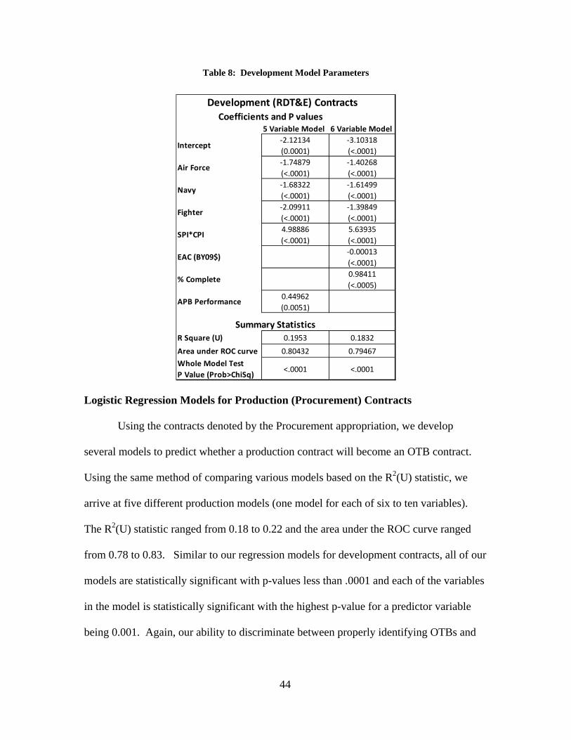
44

Table 8: Development Model Parameters

           Development (RDT&E) Contracts                   Coefficients and P values

5 Variable Model 6 Variable Model

Intercept‐2.12134

(0.0001)

‐3.10318

(<.0001)

Air Force‐1.74879

(<.0001)

‐1.40268

(<.0001)

Navy‐1.68322

(<.0001)

‐1.61499

(<.0001)

Fighter‐2.09911

(<.0001)

‐1.39849

(<.0001)

SPI*CPI4.98886

(<.0001)

5.63935

(<.0001)

EAC (BY09$)‐0.00013

(<.0001)

% Complete0.98411

(<.0005)

APB Performance0.44962

(0.0051)

                           Summary Statistics

R Square (U) 0.1953 0.1832

Area under ROC curve 0.80432 0.79467

Whole Model Test

P Value (Prob>ChiSq)<.0001 <.0001

Logistic Regression Models for Production (Procurement) Contracts

Using the contracts denoted by the Procurement appropriation, we develop

several models to predict whether a production contract will become an OTB contract.

Using the same method of comparing various models based on the R2(U) statistic, we

arrive at five different production models (one model for each of six to ten variables).

The R2(U) statistic ranged from 0.18 to 0.22 and the area under the ROC curve ranged

from 0.78 to 0.83. Similar to our regression models for development contracts, all of our

models are statistically significant with p-values less than .0001 and each of the variables

in the model is statistically significant with the highest p-value for a predictor variable

being 0.001. Again, our ability to discriminate between properly identifying OTBs and

45

not is considered to range from acceptable to excellent based on the guidelines for the

area under the ROC curve. However, the model’s ability to explain the results is low

based on the low R2(U) values.

Similar to our case for development contracts, there is not much of a difference

between the R2(U) statistic and area under the ROC curve for each of the models.

Therefore, we choose two models to consider which have fewer predictor variables. This

provides the user with a simpler model without compromising much predictive power.

Each of these models has slightly different predictors. One model contains five variables

and the other contains seven variables. The regression results for development contracts

are in Appendix E. Table 9 provides the summary output and parameters for each of

these models.

To interpret the predictor variables in each of these models the signs of the

coefficients are reversed. Contracts that have a high BCWS and a low BCWP are more

likely to experience an OTB. This means that contracts with a large amount of work

scheduled (BCWS) and a small amount of work performed (BCWP) are more likely to

experience an OTB. Contracts that have experienced a large change in the production

quantity since the initial report are more likely to experience an OTB. A contract that has

experienced an APB schedule breach is also more likely to experience an OTB. For the

five variable model, a contract with a large EAC is more likely to become an OTB. For

the six variable model, a contract with a low value for % complete (early on) and has

experienced an APB performance breach is more likely to experience an OTB.

46

Table 9: Production Model Parameters

      Production (Procurement) Contracts                 Coefficients and P values

5 Variable Model 7 Variable Model

Intercept2.99823

(<.0001)

2.45622

(<.0001)

BCWS (BY09$)‐.02918

(<.0001)

‐.03368

(<.0001)

BCWP (BY09$)0.03472

(<.0001)

0.03724

(<.0001)

MR (BY09$)‐0.01627

(<.0001)

EAC (BY09$)‐.00108

(<.0001)

% Complete1.92580

(<.0001)

% Change in 

Production Quantity

‐0.00117

(<.0001)

‐0.00140

(<.0001)

APB Schedule‐0.73515

(0.0010)

‐0.84723

(0.0002)

APB Performance‐1.07029

(<.0001)

                           Summary StatisticsR Square (U) 0.1840 0.2042

Area under ROC curve 0.78087 0.80413

Whole Model Test

P Value (Prob>ChiSq)<.0001 <.0001

Validation of Logistic Regression Models

Before coming to the conclusion that these models can be applied to predict

OTBs, we must validate their predictive ability. Using the 20% of the data that we

initially set aside, we test the performance of the final four models. Since the positive or

negative signs of the coefficients for each predictor in JMP® are the opposite of what they

would be in the standard logistic regression equation presented in Table 6 of Chapter

Three, we must adjust our logistic regression equation. For computational purposes, we

calculate the logistic regression response by using the formula in Table 10 along with the

values that JMP® provides for the coefficients B0, B1... Bn.

47

Table 10: Computational Form of Logistic Regression Equation

п(x) = e -(B0+B1x

1+ B

2x

2+…+B

nx

n)

1+e -(B0+B1x

1+B

2x

2 + …+B

nx

n)

For each entry in the validation set, we compute the logistic response, which is the

predicted likelihood that a contract will become an OTB contract. The model uses a

cutoff of 0.5 to determine whether we predict an OTB with our model. If the logistic

response is greater than 0.5, we identify the entry as a predicted OTB and code it as a

one. If the logistic response is less than 0.5, we identify the entry as not being a predicted

OTB and code it as a zero. The validation involves comparing these values with the

actual values of whether a contract becomes an OTB. When the predicted value is a one

and the actual value is a one, we correctly predict an OTB. When the predicted value is a

one and the actual value is a zero, we incorrectly predict an OTB. Table 11 provides a

summary of the validation results for the development (RDT&E) and production

(Procurement) contracts.

We first interpret the results for the development contracts (RDT&E). When an

OTB is predicted (Prediction = 1), the prediction is only correct approximately fifty

percent of the time (Prediction=1, Actual=1). Furthermore, the model frequently fails to

predict an OTB when an OTB occurs (Prediction=0, Actual=1). Based on these findings,

we conclude that these models are not good predictors of RDT&E OTB contracts.

When analyzing the results for the production contracts (Procurement), we find

that we rarely predict an OTB in comparison to the actual instances of an OTB.

However, when an OTB is predicted (Prediction=1), the prediction tends to be correct

since there are very few instances of incorrectly predicting an OTB (Prediction=1,

48

Actual=0). While this may appear to be a good outcome, the objective is to identify

OTBs. Since the models fail to identify the majority of OTBs when they occur, the

conclusion is that these models are not good predictors of Procurement OTB contracts.

Table 11: Model Validation Results

RDT&E 5 Variables

OutcomePrediction Actual Frequency

0 0 592

1 1 27

0 1 112

1 0 30

RDT&E 6 Variables

OutcomePrediction Actual Frequency

0 0 580

1 1 24

0 1 113

1 0 29

Procurement 5 Variables

OutcomePrediction Actual Frequency

0 0 587

1 1 6

0 1 51

1 0 0

Procurement 7 Variables

OutcomePrediction Actual Frequency

0 0 572

1 1 8

0 1 49

1 0 2

Recall in Chapter Three, that to determine how close the model is to accurately

predicting OTBs, we can consider how far off our predicted values are from the cut-off

point, which is 0.5. When examining the inaccurate predictions (either prediction=1 and

actual=0 or prediction=0 and actual=1), the logistic responses for these inaccurate

predictions are far from the cutoff point of 0.5. Therefore, the cutoff point that we

choose does not affect our predictive capability. Since this process of predicting OTBs

did not produce sufficient models for predicting OTBs, we seek other methods to refine

our models.

49

Additional Attempts at Predicting OTBs

One method to try to improve the model’s predictive ability is to limit the data set

to a more applicable period. In Figure 6, the box plot for the value of percent complete

one period prior to an OTB indicates that OTBs tend to occur midway through a

contract’s life. Since OTBs do not tend to occur early or late in a contract’s life, we

attempted to build models that exclude data beyond a certain value of percent complete,

specifically looking at the values of 60% and 70% complete. By excluding data points

beyond these periods, the models still lacked sufficient predictive capability. We also

considered models that only included data points in the ranges of 10-60% complete and

20-70% complete. Again, neither of these models produced significant results.

Figure 6: Box Plot of % Complete Prior to OTB

A second method is to search for trends in OTB contracts. By identifying a

common trend, we can see if this trend exists in non-OTB contracts. Since the OTB

process is not a mandatory process, it is possible to flag non-OTB contracts as contracts

50

that were candidates for an OTB. Then we can develop new models that incorporate the

identification of OTBs along with OTB candidate contracts. Unfortunately, we were

unable to identify any common trends among the OTB contracts. This suggests that the

process of identifying contracts to become OTB may be random since the OTB process is

an optional step.

Finally, there is an alternative method for identifying OTBs. All of the previous

models use the standard definition of an OTB provided by DAU, which defines an OTB

based on the TAB exceeding the CBB. However, the DAES database also has a data

field that identifies an OTB when the program office reports an OTB in the DAES

database. When we rerun our models based on this alternative way of identifying an

OTB, we obtain similar results to what we have already found: correct OTB predictions

approximately half of the time and the failure to predict the majority of OTBs. This

alternative also fails to provide better predictive capabilities.

Conclusion

After the initial model building attempts that considered all of the available

predictors, interactions between predictors, and changes in predictors along with the

additional attempts to develop predictive models, we conclude that the models are unable

to predict OTBs based on the data available to us. In the next chapter, we discuss the

implications of these findings.

51

V: Discussion and Conclusion

In this chapter, we recall the purpose of this thesis and the results from the

analysis. We discuss the implication of our results and what policy implications our

results provide. Finally, we suggest some potential areas for future research related to

earned value management.

Thesis Purpose

In 2009, Captain Trahan developed a growth model, which improves EACs for

contracts that are Over Target Baselines (OTBs). To apply this model to improve EACs,

the contract must be an OTB or it must become an OTB in the future. This thesis

attempts to predict OTB contracts with the intent of applying Captain Trahan’s model to

develop better EACs. By improving EACs, cost estimators provide the DoD with the

capability to provide more content to the war fighter. A high EAC limits the ability to

acquire additional capabilities with the additional (unnecessary) funds allotted to a

program. A low EAC creates problems for the program with a low estimate since it will

require additional funds to deploy that capability to the field. Furthermore, when one

program has too low of an EAC, the services (Army, Navy, Air Force, etc.) tend to

borrow money from other programs and this causes problems for all of the programs

involved. In addition to improving EACs, the ability to predict OTBs allows decision

makers to identify cost overruns since an OTB formally recognizes cost overruns.

Summary of Results

We built separate logistic regression models to predict OTB contracts for

production and development contracts and chose four models to use based on an

52

evaluation of the predictive capabilities for each of the models. These models contain

five to seven predictor variables capturing EVM metrics, production information, and

threshold breach information. While we were able to develop significant models for the

model building set, all of the models failed in the validation stage. The validation results

indicate that the ability to predict OTBs is no better than a coin flip. Furthermore, the

models fail to predict the majority of OTBs when they occur. Since our objective is to

identify OTBs, the failure to predict an OTB is substantial. Additional attempts at

refining the model based on the definition of an OTB and the period considered also

proved unsuccessful. Based on these results, we are unable to predict an OTB.

However, in one of the attempts, we examine a variety of predictor variables from

the regression models. In this analysis, there were no common trends in these variables

for OTB contracts. This is an important observation as it suggests that OTBs may occur

randomly, which would explain the inability to predict OTBs.

Policy Implications

Since OTBs are not required and contractors conduct OTBs at their discretion,

contractors may not utilize the OTB process when it may be beneficial to them.

Furthermore, the limited number of OTB contracts limits the amount of cost overruns that

the DoD can quantify. Without the use of OTBs, decision makers can identify cost

growth, but the ability to quantify cost overruns becomes much more difficult.

Perhaps contractors could be required to distinguish between increased costs due

to requirement changes and increased costs due to cost overruns or contract performance

issues. This topic needs to be addressed carefully as contractors are less likely to report

contract performance issues and are more likely to report increased costs due to

53

requirement changes. One option is to require contractors to estimate the costs of the

specific requirement changes opposed to presenting a revised single estimate for the

entire program when a requirement change occurs. Another way to prevent contractors

from hiding cost overruns in a new baseline would be to require contract changes be

implemented in a follow on increment or to use a spiral acquisition strategy.

The ability to identify cost overruns separately from cost growth allows decision

makers to measure a contractor’s performance. If the DoD can require contractors to

report cost overruns or create an environment that prevents contractors from hiding

overruns, such as with a spiral acquisition strategy, the DoD could better evaluate and

manage contractor performance. With increased visibility into the costs incurred by the

DoD, cost estimators could identify the reasons for increased costs and recommend

actions to control costs.

Future Research

The OTB process appears to be random within the DoD. So decision makers

must ask the question, why do contractors use it? The DAU guide on OTBs explains the

purpose of an OTB, but it does not quantify the benefits realized for OTB contracts. One

possible research topic would be to quantify the benefits of a contract going through the

OTB process versus not going through the OTB process. This would determine if the

process is worthwhile or not.

Additionally, in the process of collecting data, we discovered that the DCARC

database has more detailed CPR data available along with the original CPR submissions.

Researchers should use the DCARC database for studies that require EVM data on recent

contracts since the data is more reliable. However, since the database only includes

54

entries back to 2007, researchers should wait until more data becomes available to

conduct extensive studies.

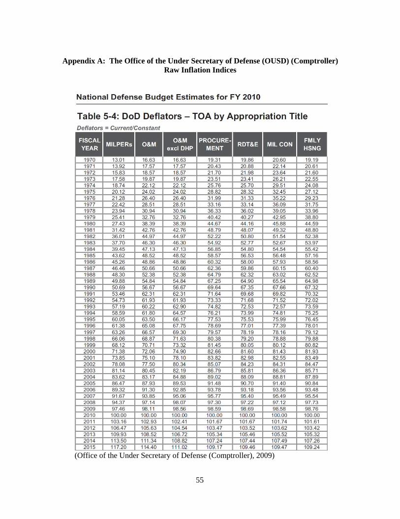
55

Appendix A: The Office of the Under Secretary of Defense (OUSD) (Comptroller)

Raw Inflation Indices

(Office of the Under Secretary of Defense (Comptroller), 2009)

56

Appendix B: The Office of the Under Secretary of Defense OUSD (Comptroller)

Outlay Rates

Table 5-11: Outlay Rates for Incremental Changes in BA Purchases

Outlay Profiles: 1st Year 2nd Year 3rd Year 4th Year 5th Year 6th Year 7th YearProcurement (Defense Wide) 0.23 0.41 0.25 0.07 0.02 0.01 0.01RDT&E (Defense Wide) 0.44 0.43 0.07 0.04 0.01 0.01O&M (Defense Wide) 0.51 0.40 0.05 0.02 0.01 0.01

(Office of the Under Secretary of Defense (Comptroller), 2009)

57

Appendix C: Weighted Inflation Indices

Weighted Indices (base year of table: 2009)Procurement RDT&E O&M

1970 21.20 20.95 17.571971 22.67 22.10 18.601972 24.55 23.49 19.821973 26.95 25.43 21.561974 29.78 27.94 23.741975 32.57 30.75 25.901976 35.02 33.35 28.251977 37.97 35.86 30.581978 41.89 39.44 32.981979 46.06 43.54 36.381980 50.00 47.35 41.441981 53.37 50.61 44.831982 56.04 52.96 46.641983 58.15 54.95 47.781984 60.01 56.85 48.861985 61.91 58.54 49.891986 64.03 60.32 50.981987 66.38 62.53 52.831988 68.79 65.06 54.911989 71.06 67.56 57.241990 73.06 69.89 60.411991 74.76 71.96 63.261992 76.26 73.43 62.491993 77.65 74.63 62.411994 78.92 76.12 64.071995 80.04 77.61 65.751996 81.01 78.92 67.381997 81.96 80.04 69.261998 83.05 81.05 71.391999 84.26 82.29 73.152000 85.56 83.78 75.322001 87.03 85.19 78.172002 88.84 86.74 80.902003 91.02 88.75 83.912004 93.35 91.21 87.522005 95.56 93.72 91.652006 97.48 96.02 94.692007 99.09 98.01 97.502008 100.53 99.66 99.832009 102.04 101.12 101.352010 N/A 102.68 103.78

58

Appendix D: Logistic Regression Models: Development Contracts

Difference

Full

Reduced

Model

221.5882

912.7929

1134.3810

-LogLikelihood

5

DF

443.1763

ChiSquare

<.0001*

Prob>ChiSq

RSquare (U)

Observations (or Sum Wgts)

0.1953

2257

Converged by Gradient

Whole Model Test

Lack Of Fit

Saturated

Fitted

Source

2081

2086

5

DF

888.05881

24.73404

912.79285

-LogLikelihood

1776.118

ChiSquare

1.0000

Prob>ChiSq

Lack Of Fit

Intercept

Air Force

Navy

Fighter=1

SPI*CPI

APB Perf (since program began)

Term

-2.1213432

-1.7487887

-1.6832163

-2.0991097

4.98886162

0.44961724

Estimate

0.5481341

0.1512736

0.1468049

0.1732385

0.6015667

0.1604091

Std Error

14.98

133.64

131.46

146.82

68.78

7.86

ChiSquare

0.0001*

<.0001*

<.0001*

<.0001*

<.0001*

0.0051*

Prob>ChiSq

For log odds of 0/1

Parameter Estimates

Air Force

Navy

Fighter=1

SPI*CPI

APB Perf (since program began)

Source

1

1

1

1

1

Nparm

1

1

1

1

1

DF

139.223595

136.948261

153.323909

74.0553979

8.22450541

L-R

ChiSquare

<.0001*

<.0001*

<.0001*

<.0001*

0.0041*

Prob>ChiSq

Effect Likelihood Ratio Tests

Tru

e P

ositi

ve

Sen

sitiv

ity

0.00

0.10

0.20

0.30

0.40

0.50

0.60

0.70

0.80

0.90

1.00

0.00 0.20 0.40 0.60 0.80 1.00

1-Specificity

False Positive

Using Will it become an OTB? (yes=1, no=0)='1' to be the positive level

Area Under Curve = 0.80432

Receiver Operating Characteristic

Nominal Logistic Fit for Will it become an OTB? (yes=1, no=0)

59

Difference

Full

Reduced

Model

246.0426

1096.6904

1342.7330

-LogLikelihood

6

DF

492.0853

ChiSquare

<.0001*

Prob>ChiSq

RSquare (U)

Observations (or Sum Wgts)

0.1832

2809

Converged by Gradient

Whole Model Test

Lack Of Fit

Saturated

Fitted

Source

2646

2652

6

DF

1081.4411

15.2492

1096.6904

-LogLikelihood

2162.882

ChiSquare

1.0000

Prob>ChiSq

Lack Of Fit

Intercept

Air Force

Navy

Fighter=1

SPI*CPI

EAC (BY09$)

% Complete

Term

-3.1031811

-1.4026827

-1.6149947

-1.3984851

5.63935418

-0.0001286

0.98410535

Estimate

0.4946008

0.139231

0.1326298

0.1767598

0.5434839

0.0000208

0.1966273

Std Error

39.36

101.50

148.27

62.60

107.67

38.27

25.05

ChiSquare

<.0001*

<.0001*

<.0001*

<.0001*

<.0001*

<.0001*

<.0001*

Prob>ChiSq

For log odds of 0/1

Parameter Estimates

Air Force

Navy

Fighter=1

SPI*CPI

EAC (BY09$)

% Complete

Source

1

1

1

1

1

1

Nparm

1

1

1

1

1

1

DF

99.577974

152.01374

59.5560043

115.885391

44.7105976

25.307887

L-R

ChiSquare

<.0001*

<.0001*

<.0001*

<.0001*

<.0001*

<.0001*

Prob>ChiSq

Effect Likelihood Ratio Tests

Tru

e P

ositi

ve

Sen

sitiv

ity

0.00

0.10

0.20

0.30

0.40

0.50

0.60

0.70

0.80

0.90

1.00

0.00 0.20 0.40 0.60 0.80 1.00

1-Specificity

False Positive

Using Will it become an OTB? (yes=1, no=0)='1' to be the positive level

Area Under Curve = 0.79467

Receiver Operating Characteristic

Nominal Logistic Fit for Will it become an OTB? (yes=1, no=0)

60

Appendix E: Logistic Regression Models: Production Contracts

Difference

Full

Reduced

Model

107.62019

477.20578

584.82597

-LogLikelihood

5

DF

215.2404

ChiSquare

<.0001*

Prob>ChiSq

RSquare (U)

Observations (or Sum Wgts)

0.1840

2153

Converged by Gradient

Whole Model Test

Lack Of Fit

Saturated

Fitted

Source

2068

2073

5

DF

477.20578

0.00000

477.20578

-LogLikelihood

954.4116

ChiSquare

1.0000

Prob>ChiSq

Lack Of Fit

Intercept

BCWS (BY09$)

BCWP (BY09$)

EAC (BY09$)

%Change in Prod Qty

APB Sched (since program began)

Term

2.99823206

-0.0291836

0.03472149

-0.0010841

-0.0011729

-0.7351471

Estimate

0.2113997

0.0037638

0.0039848

0.0001488

0.0001372

0.2228897

Std Error

201.15

60.12

75.92

53.06

73.12

10.88

ChiSquare

<.0001*

<.0001*

<.0001*

<.0001*

<.0001*

0.0010*

Prob>ChiSq

For log odds of 0/1

Parameter Estimates

BCWS (BY09$)

BCWP (BY09$)

EAC (BY09$)

%Change in Prod Qty

APB Sched (since program began)

Source

1

1

1

1

1

Nparm

1

1

1

1

1

DF

64.2231264

84.6860049

48.8409568

71.5295638

11.9958743

L-R

ChiSquare

<.0001*

<.0001*

<.0001*

<.0001*

0.0005*

Prob>ChiSq

Effect Likelihood Ratio Tests

Tru

e P

ositi

ve

Sen

sitiv

ity

0.00

0.10

0.20

0.30

0.40

0.50

0.60

0.70

0.80

0.90

1.00

0.00 0.20 0.40 0.60 0.80 1.00

1-Specificity

False Positive

Using Will it become an OTB? (yes=1, no=0)='1' to be the positive level

Area Under Curve = 0.78087

Receiver Operating Characteristic

Nominal Logistic Fit for Will it become an OTB? (yes=1, no=0)

61

Difference

Full

Reduced

Model

119.64819

466.27867

585.92686

-LogLikelihood

7

DF

239.2964

ChiSquare

<.0001*

Prob>ChiSq

RSquare (U)

Observations (or Sum Wgts)

0.2042

2136

Converged by Gradient

Whole Model Test

Lack Of Fit

Saturated

Fitted

Source

2053

2060

7

DF

466.27867

0.00000

466.27867

-LogLikelihood

932.5573

ChiSquare

1.0000

Prob>ChiSq

Lack Of Fit

Intercept

BCWS (BY09$)

BCWP (BY09$)

MR (BY09$)

% Complete

%Change in Prod Qty

APB Sched (since program began)

APB Perf (since program began)

Term

2.45621515

-0.0336802

0.03724202

-0.0162715

1.92580313

-0.0013979

-0.8472259

-1.0702907

Estimate

0.2135546

0.0038816

0.0041528

0.0026889

0.3488721

0.0001473

0.2239202

0.2110283

Std Error

132.29

75.29

80.42

36.62

30.47

90.04

14.32

25.72

ChiSquare

<.0001*

<.0001*

<.0001*

<.0001*

<.0001*

<.0001*

0.0002*

<.0001*

Prob>ChiSq

For log odds of 0/1

Parameter Estimates

BCWS (BY09$)

BCWP (BY09$)

MR (BY09$)

% Complete

%Change in Prod Qty

APB Sched (since program began)

APB Perf (since program began)

Source

1

1

1

1

1

1

1

Nparm

1

1

1

1

1

1

1

DF

80.1344568

90.5358401

15.7144622

33.6027505

89.0189208

15.7997568

23.7841223

L-R

ChiSquare

<.0001*

<.0001*

<.0001*

<.0001*

<.0001*

<.0001*

<.0001*

Prob>ChiSq

Effect Likelihood Ratio Tests

Tru

e P

ositi

ve

Sen

sitiv

ity

0.00

0.10

0.20

0.30

0.40

0.50

0.60

0.70

0.80

0.90

1.00

0.00 0.20 0.40 0.60 0.80 1.00

1-Specificity

False Positive

Using Will it become an OTB? (yes=1, no=0)='1' to be the positive level

Area Under Curve = 0.80413

Receiver Operating Characteristic

Nominal Logistic Fit for Will it become an OTB? (yes=1, no=0)

62

Bibliography

Abrams, Jim. “Senate passes acquisition reform legislation,” The Air Force Times, 7 May 2009. Air Force Cost Analysis Agency. Air Force Cost Analysis Handbook. Washington: March 2007. Bielecki, John V. and Edward D. White, III. “Estimating Cost Growth From Schedule Changes: A Regression,” Cost Engineering, 47: 28-34 (August 2005). Christensen, David S. “Using Performance Indices to Evaluate the Estimate at Completion,” Journal of Cost Analysis, (Spring 1994). Christensen, David S. “Value Cost Management Report to Evaluate the Contractor’s Estimate at Completion,” Acquisition Review Quarterly, 283:295 (Summer 1999). Christensen, David S., Richard D. Antolini, John W. McKinney, and The Air Force Institute of Technology. “A Review of Estimate at Completion Research,” Journal of Cost Analysis, 41:62 (Spring 1995). Cukr, Anita. “When is an Over Target Baseline (OTB) Necessary?” The Measurable News, (March 2001). Dahl, Joachim and Lieven Vandenberghe. “Logistic Regression (Fig 7.1),” Figure from course information. http://abel.ee.ucla.edu/cvxopt/examples/book/logreg.html. 31 July 2009. Defense Acquisition University (DAU). Earned Value Management ‘Gold Card.’ January 2009. Defense Acquisition University (DAU). Over Target Baseline and Over Target Schedule Handbook. 7 May 2003. Department of Defense. Defense Federal Acquisition Regulation Supplement: Earned Value Management System. Subpart 234.2. Washington: OUSD (AT&L), 21 July 2009. Genest, Daniel C. and Edward D. White, III. “Predicting RDT&E Cost Growth,” The Journal of Cost Analysis and Management, 1:12 (Fall 2005). GSA FAR Secretariat. Federal Acquisition Regulation: Earned Value Management System. Subpart 34.2. Washington: GSA, 15 July 2009.

63

Hosmer, David W. and Stanley Lemeshow. Applied Logistic Regression. New York: John Wiley & Sons, 2000. JMP®. Version 8. (Academic) computer software. Cary, NC: SAS Institute Inc., 2009. Monaco, James V and Edward D. White, III. “Extending Cost Growth Estimation to Predict Schedule Risk,” The Journal of Cost Analysis and Management, 1:13 (Fall 2006). Neter, John, Michael H. Kutner, Christopher J. Nachtsheim, and William Wassermanl. Applied Linear Statistical Models. Boston: McGraw-Hill, 1996. Office of the Under Secretary of Defense (Comptroller). National Defense Budget Estimates for FY10 (Green Book). Washington: DoD, June 2009. Rosetti, Matthew B. and Edward D. White, III. “A Two-Pronged Approach to Estimate Procurement Cost Growth in Major DoD Weapon Systems,” The Journal of Cost Analysis and Management, 11:21 (Winter 2004). Tiffany, Dorothy, Program Business Manager, National Aeronautics and Space Administration, Goddard Space Flight Center. “The Over Target Baseline (OTB).” Presentation at the 20th Annual PMI-CPM International Conference. 13 May 2004. Tracy, Steven P. Estimate at Completion: A Regression Approach to Earned Value. MS Thesis, AFIT/GCA/ENC/05-04. Graduate School of Engineering and Management, Air Force Institute of Technology (AU), Wright Patterson AFB OH, March 2005. Trahan, Elizabeth. An Evaluation of Growth Models as Predictive Tools for Estimates at Completion (EAC). MS Thesis, AFIT/GFA/ENC/09-01. Graduate School of Engineering and Management, Air Force Institute of Technology (AU), Wright Patterson AFB OH, March 2009. White, Edward D., III, Vincent P. Sipple, and Michael A. Greiner. “Using Logistic and Multiple Regression to Estimate Engineering Cost Risk,” The Journal of Cost Analysis and Management, 67:79 (Summer 2004).

64

Vita

Captain Kristine Thickstun attended Miami University (OH) where she graduated

Magna Cum Laude in 2005 with a Bachelor of Science degree in Mathematics and a

minor in Economics. In May of 2005, she received a commission as a 2nd Lt in the Air

Force out of the AFROTC program.

Upon commissioning, she reported to headquarters Air Education and Training

Command (AETC), Randolph AFB, Texas. She worked at the Studies and Analysis

Squadron within AETC A5/8/9 as a scientist. During her three-year assignment she

supported the command on technical training studies, flying training studies, pilot

selection studies, cost studies, and a variety of AETC initiatives.

While serving at Randolph AFB, Captain Thickstun was a student in the MBA

program at St. Mary’s University in San Antonio, Texas. In 2008, she graduated as a

distinguished graduate with an emphasis in financial planning. For her academic

achievements at St. Mary’s University, she was chosen as the 2008 St. Mary’s University

recipient of the Texas Business Hall of Fame Scholarship, an award given to 16 graduate

students in Texas.

In August of 2008, she entered the Cost Analysis program at the Air Force

Institute of Technology. Upon graduation, she will be assigned to Los Angeles AFB,

CA.

REPORT DOCUMENTATION PAGEForm Approved OMB No. 074-0188

The public reporting burden for this collection of information is estimated to average 1 hour per response, including the time for reviewing instructions, searching existing data sources, gathering and maintaining the data needed, and completing and reviewing the collection of information. Send comments regarding this burden estimate or any other aspect of the collection of information, including suggestions for reducing this burden to Department of Defense, Washington Headquarters Services, Directorate for Information Operations and Reports (0704-0188), 1215 Jefferson Davis Highway, Suite 1204, Arlington, VA 22202-4302. Respondents should be aware that notwithstanding any other provision of law, no person shall be subject to an penalty for failing to comply with a collection of information if it does not display a currently valid OMB control number. PLEASE DO NOT RETURN YOUR FORM TO THE ABOVE ADDRESS. 1. REPORT DATE (DD-MM-YYYY) 25-03-2010

2. REPORT TYPE Master’s Thesis

3. DATES COVERED (From – To) June 2009 – March 2010

4. TITLE AND SUBTITLE Predicting Over Target Baseline (OTB) Acquisition Contracts

5a. CONTRACT NUMBER

5b. GRANT NUMBER

5c. PROGRAM ELEMENT NUMBER

6. AUTHOR(S) Thickstun, Kristine E., Captain, USAF

5d. PROJECT NUMBER

5e. TASK NUMBER

5f. WORK UNIT NUMBER

7. PERFORMING ORGANIZATION NAMES(S) AND ADDRESS(S) Air Force Institute of Technology Graduate School of Engineering and Management (AFIT/EN) 2950 Hobson Way WPAFB OH 45433-7765

8. PERFORMING ORGANIZATION REPORT NUMBER

AFIT/GCA/ENC/10-01

9. SPONSORING/MONITORING AGENCY NAME(S) AND ADDRESS(ES) Gaile Argiro Executive Administrator PMI College of Performance Management 101 S. Whiting Street, Suite 320 Alexandria, Virginia 22304

10. SPONSOR/MONITOR’S ACRONYM(S) PMI-CPM 11. SPONSOR/MONITOR’S REPORT NUMBER(S)

12. DISTRIBUTION/AVAILABILITY STATEMENT APPROVED FOR PUBLIC RELEASE; DISTRIBUTION UNLIMITED 13. SUPPLEMENTARY NOTES 14. ABSTRACT Cost estimators use a variety of methods to develop estimates at completion (EACs) and new methods continue to be developed. Research has shown there is no best method for computing EACs for all acquisition contracts. However, some methods perform better under specific circumstances. In 2009, Captain Trahan investigated the use of a Gompertz growth model for developing EACs. She found that this method is more reliable for Over Target Baseline (OTB) contracts than the standard indexed based approaches. Captain Trahan’s model is an excellent model to use for OTB contracts or contracts with a high likelihood of becoming an OTB contract. In this study, we attempt to develop a model that predicts whether an acquisition contract is likely to become an OTB. By identifying contracts that are likely to become OTB, we can apply the Gompertz growth model to develop better EACs. Furthermore, an OTB, by definition, recognizes a cost overrun. Therefore, the ability to predict OTBs also allows us to understand what may cause cost overruns. However, our models indicate that we are unable to predict an OTB. This indicates that the OTB process may be used randomly which leads us to question the benefits of OTBs. 15. SUBJECT TERMS Over Target Baseline (OTB), Earned Value Management (EVM), Estimate at Completion (EAC), cost overruns, logistic regression

16. SECURITY CLASSIFICATION OF: 17. LIMITATION OF ABSTRACT UU

18. NUMBER OF PAGES

75

19a. NAME OF RESPONSIBLE PERSON Dr. Edward D. White (AFIT/ENC)

a. REPORT

U

b. ABSTRACT

U

c. THIS PAGE

U

19b. TELEPHONE NUMBER (Include area code) 937-785-3636 ext. 4540 EMAIL: EDWARD.WHITE@AFIT.EDU

Standard Form 298 (Rev. 8-98) Prescribed by ANSI Std. Z39-18

Form Approved OMB No. 074-0188