1

Predicting Market Value of Soccer Players

Using Linear Modeling Techniques

by Yuan He

Advisor: David Aldous

Index

Introduction ---------------------------------------------------------------------------- 2

Description of Data -------------------------------------------------------------------- 3

Preliminary Analysis ------------------------------------------------------------------ 5

Model Selection ------------------------------------------------------------------------ 8

Prediction and Discussion ------------------------------------------------------------ 10

Future Developments ------------------------------------------------------------------ 13

Conclusion ------------------------------------------------------------------------------ 14

References ------------------------------------------------------------------------------ 14

2

Introduction

Sports data has been a popular topic for statisticians in the recent years. People study various

data in many different ball games and draw conclusions based on their analysis. Soccer, known

to be the most popular sport on this planet, failed to appear in most of the statistical studies for it

is difficult to collect and organize data regarding this sport. Unlike basketball or American

football, where the existence of a sole professional league (NBA and NFL) makes it easy to

record everything, soccer is played all around the world with so many leagues and tournaments

to consider about. Nowadays, the appearance of professional soccer statistics websites has made

it possible to extent statistical study to the field of soccer.

Besides goals and silverwares, soccer fans find transfer stories exciting. Transfers involving top

players with high market value never failed to hit the headlines. Market value varies greatly for

different players, different areas and different periods of time. As Sir Alex Ferguson stated in his

autobiography: "I advanced from managing East Stirling players on 6 pounds a week to selling

Cristiano Ronaldo to Real Madrid for 80 million pounds." (Ferguson, 16). It is thus interesting to

study various factors that could influence market value of soccer players. In the world of soccer,

a German website, transfermarkt.de, is the authority in judging market value of soccer players.

This website records detailed information for major soccer players and evaluate their value based

on data analysis, as well as opinions of experts. The values are not obtained by applying

straightforward algorithms. Instead, factors from all aspects have to be taken into considerations

to decide the digits of a market value.

This project focuses on predicting market value of top players using statistical modeling

techniques. This aim will be achieved in three steps. Step one, data will be collected and

organized into dependent variable (i.e. market value) and independent variables (i.e. predictors);

step two, various models will be tested and evaluated; step three, predictions will be made via the

best model and accuracy of prediction will be checked.

3

Description of Data

Data were collected manually from two websites: value and personal information was collected

via transfermarkt.de; annual performance data was collected from the Wikipedia page of player.

Then a data frame was constructed in R.

The data frame has 357 rows, each representing data of a specific player over an entire season

(year). On average, data from five consecutive seasons was recorded for each player. The data

frame has 17 columns, with the first column being the value of the player at the end of that

season, in millions of Euros, given by transfermarkt.de. The rest 16 columns served as predictors.

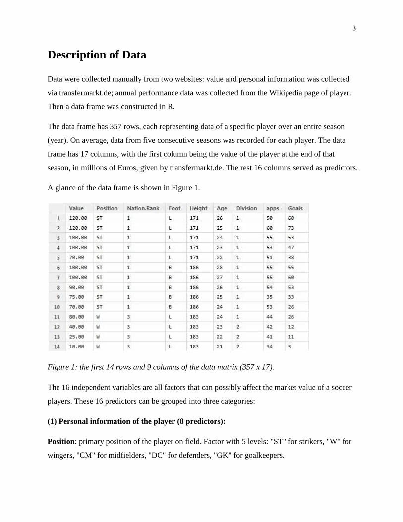
A glance of the data frame is shown in Figure 1.

Figure 1: the first 14 rows and 9 columns of the data matrix (357 x 17).

The 16 independent variables are all factors that can possibly affect the market value of a soccer

players. These 16 predictors can be grouped into three categories:

(1) Personal information of the player (8 predictors):

Position: primary position of the player on field. Factor with 5 levels: "ST" for strikers, "W" for

wingers, "CM" for midfielders, "DC" for defenders, "GK" for goalkeepers.

4

Nation.Rank: a rank of the player's national team. Factor with 3 levels: "1"-his national team is

among the best in this world; "2"-his national team qualifies for World Cup regularly, but is

never considered as the major contender; "3"-his national team rarely made it into the World Cup.

Foot: dominant foot of the player. Factor with 3 levels: "L" for left foot; "R" for right foot; "B"

for both.

Height: height of the player in centimeters. Numeric.

Age: age of the player at the point of recording value. Numeric.

Int.Caps (L.Int.Caps): International caps of the player at the end of this season (last season).

This is a measure of the player's reputation. Predictors with an "L." suffix are data from last

season.

L.Value: Market value of the player one year ago.

(2) Performance data of the player (5 predictors):

Division: A measure of the club that the player is playing for over the season. Factor with 3

levels: "1"-Famous European clubs, top 10 level in Europe; "2"-clubs with continental reputation,

clubs in major leagues; "3"-small clubs, clubs in minor leagues.

Apps (L.Apps): Appearances of the player in current season (last season). This included all

appearances in club games, whether they are league games or cup games. Appearances for

national teams were not included.

Goals (L.Goals): Goals of the player in current season (last season). This variable records all the

goals that the player scored in club games.

(3) Ratios of predictors (these were included because linear modeling only deals with linear

combinations of predictors. Ratios are not linear.):

Goal.rate (L.Goal.rate): #of goals per game of this season (last season). A ratio of Goals

(L.Goals) to Apps (L.Apps).

5

Int.age: A ratio of international caps to player's age. This is a measure of when the player

became famous in his career. Some rose to fame before 20, some emerged after 30.

Preliminary Analysis

The relationship between the dependent variable and several factors was first studied via data

visualization:

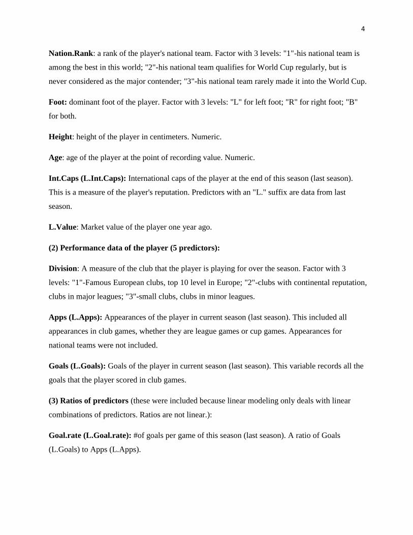
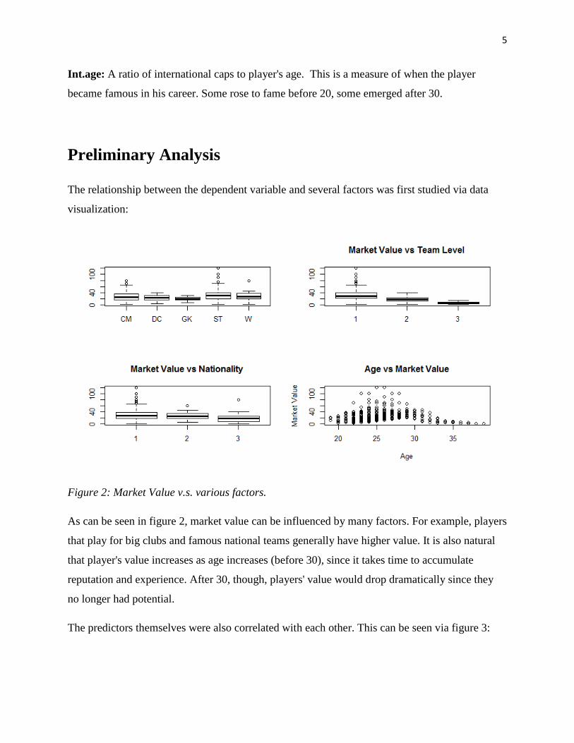
Figure 2: Market Value v.s. various factors.

As can be seen in figure 2, market value can be influenced by many factors. For example, players

that play for big clubs and famous national teams generally have higher value. It is also natural

that player's value increases as age increases (before 30), since it takes time to accumulate

reputation and experience. After 30, though, players' value would drop dramatically since they

no longer had potential.

The predictors themselves were also correlated with each other. This can be seen via figure 3:

6

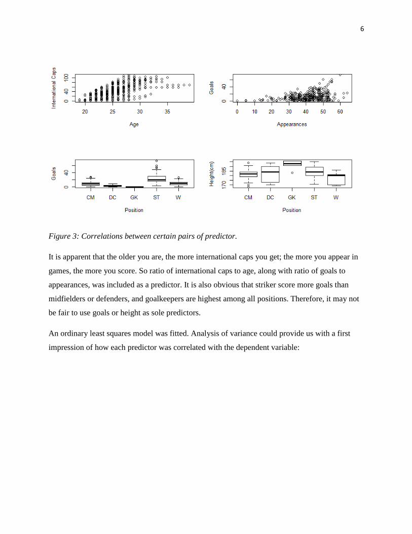
Figure 3: Correlations between certain pairs of predictor.

It is apparent that the older you are, the more international caps you get; the more you appear in

games, the more you score. So ratio of international caps to age, along with ratio of goals to

appearances, was included as a predictor. It is also obvious that striker score more goals than

midfielders or defenders, and goalkeepers are highest among all positions. Therefore, it may not

be fair to use goals or height as sole predictors.

An ordinary least squares model was fitted. Analysis of variance could provide us with a first

impression of how each predictor was correlated with the dependent variable:

7

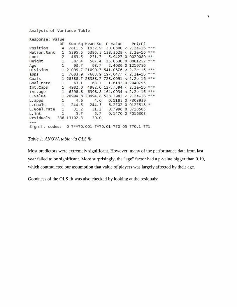
Table 1: ANOVA table via OLS fit

Most predictors were extremely significant. However, many of the performance data from last

year failed to be significant. More surprisingly, the "age" factor had a p-value bigger than 0.10,

which contradicted our assumption that value of players was largely affected by their age.

Goodness of the OLS fit was also checked by looking at the residuals:

8

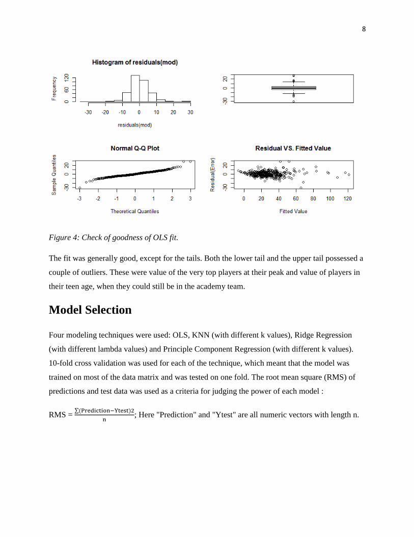
Figure 4: Check of goodness of OLS fit.

The fit was generally good, except for the tails. Both the lower tail and the upper tail possessed a

couple of outliers. These were value of the very top players at their peak and value of players in

their teen age, when they could still be in the academy team.

Model Selection

Four modeling techniques were used: OLS, KNN (with different k values), Ridge Regression

(with different lambda values) and Principle Component Regression (with different k values).

10-fold cross validation was used for each of the technique, which meant that the model was

trained on most of the data matrix and was tested on one fold. The root mean square (RMS) of

predictions and test data was used as a criteria for judging the power of each model :

RMS = ∑

; Here "Prediction" and "Ytest" are all numeric vectors with length n.

9

Original

(10 predictors)

Last Year Data

Added

(13 predictors)

Ratios Added

(16 predictors)

OLS 135.12 45.53 43.36

knn >200 ignored ignored

Ridge Regression

Lambda=1 135.044 45.382 43.44

Lambda=3 135.169 45.454 43.82

Lambda=5 135.097 45.411 44.07

Lambda=10 135.479 45.515 44.37

PCR

K=1 313.94 297.52 298.24

K=5 167.23 74.23 74.12

K=9 135.052 45.075 45.09

K=11 N/A 45.72 45.70

K=15 N/A N/A 43.29

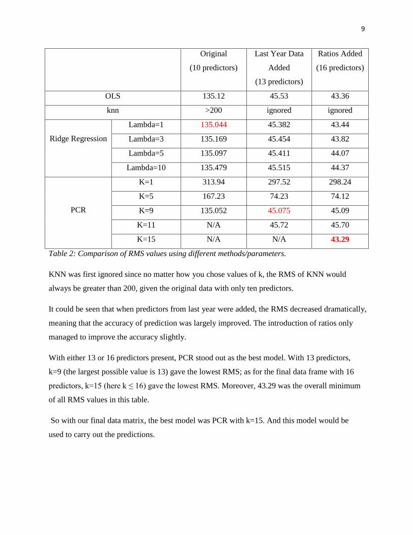
Table 2: Comparison of RMS values using different methods/parameters.

KNN was first ignored since no matter how you chose values of k, the RMS of KNN would

always be greater than 200, given the original data with only ten predictors.

It could be seen that when predictors from last year were added, the RMS decreased dramatically,

meaning that the accuracy of prediction was largely improved. The introduction of ratios only

managed to improve the accuracy slightly.

With either 13 or 16 predictors present, PCR stood out as the best model. With 13 predictors,

k=9 (the largest possible value is 13) gave the lowest RMS; as for the final data frame with 16

predictors, k=15 (here k ≤ 16) gave the lowest RMS. Moreover, 43.29 was the overall minimum

of all RMS values in this table.

So with our final data matrix, the best model was PCR with k=15. And this model would be

used to carry out the predictions.

10

Prediction and Discussion

In order to check the accuracy of our picked model. A new data frame consisting of 47 rows

(data from 10 different players) was constructed and would be used as test data. Four prediction

methods were used and RMS of each method was calculated:

Method 1: Take the overall mean as the sole prediction. If the overall mean is, say, 23. Then the

prediction vector will simply be (23,23,23,....,23) of length 47.

Method 2: Take the respective means for each player. If player I has mean value 15 and player 2

has mean value 33, etc. Then the prediction vector would be (15,15,15,15,15,33,33,33,33,33,....)

and has length 47.

Method 3: Use value from last year as the prediction. For each row, the prediction will simply be

the number within the column "L.Value".

Method 4: Use our picked model, Principle Component Regression with k = 15. The model was

trained by the whole original data matrix, without cross validation.

An evaluation of each method was carried out by calculating the corresponding RMS and

comparison of the four methods could be seen in the following table:

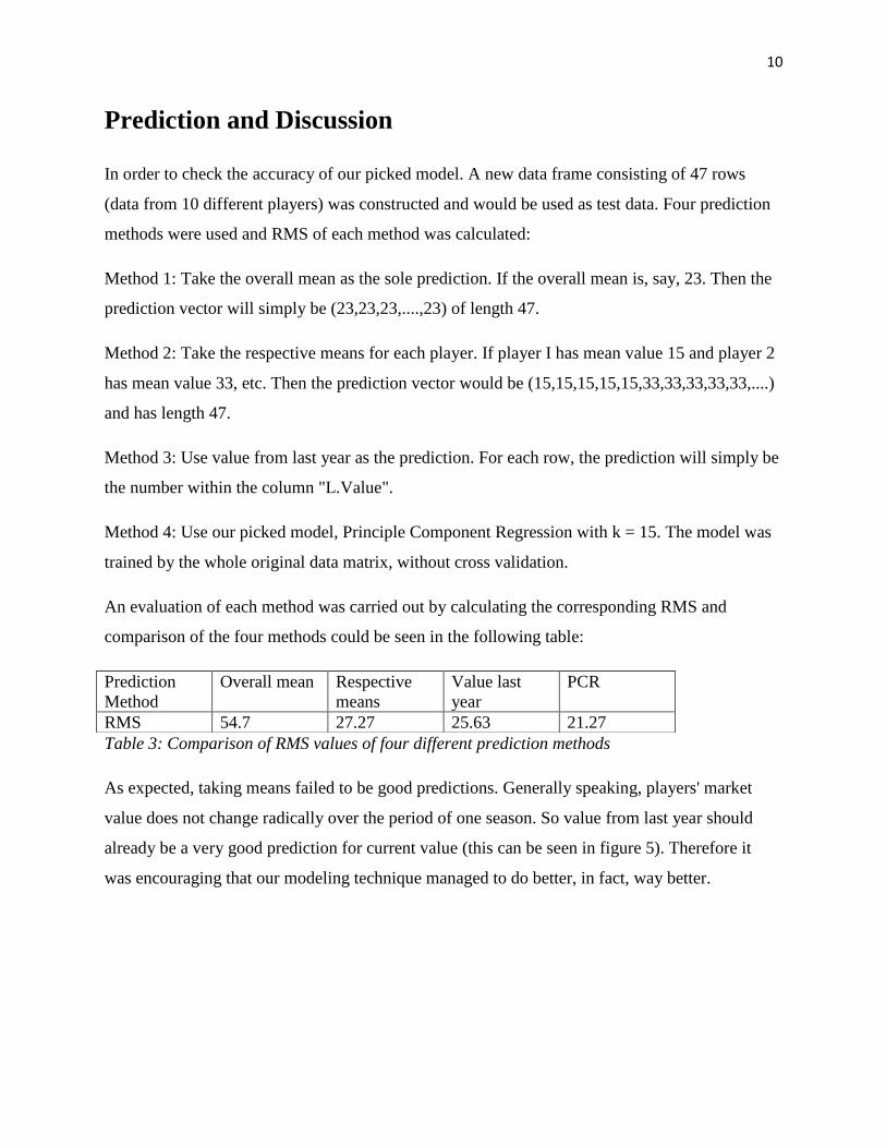
Table 3: Comparison of RMS values of four different prediction methods

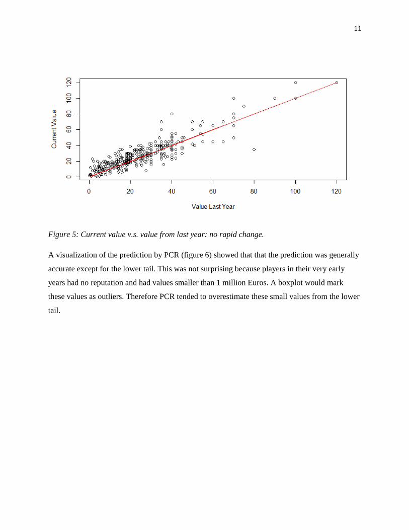
As expected, taking means failed to be good predictions. Generally speaking, players' market

value does not change radically over the period of one season. So value from last year should

already be a very good prediction for current value (this can be seen in figure 5). Therefore it

was encouraging that our modeling technique managed to do better, in fact, way better.

Prediction

Method

Overall mean Respective

means

Value last

year

PCR

RMS 54.7 27.27 25.63 21.27

11

Figure 5: Current value v.s. value from last year: no rapid change.

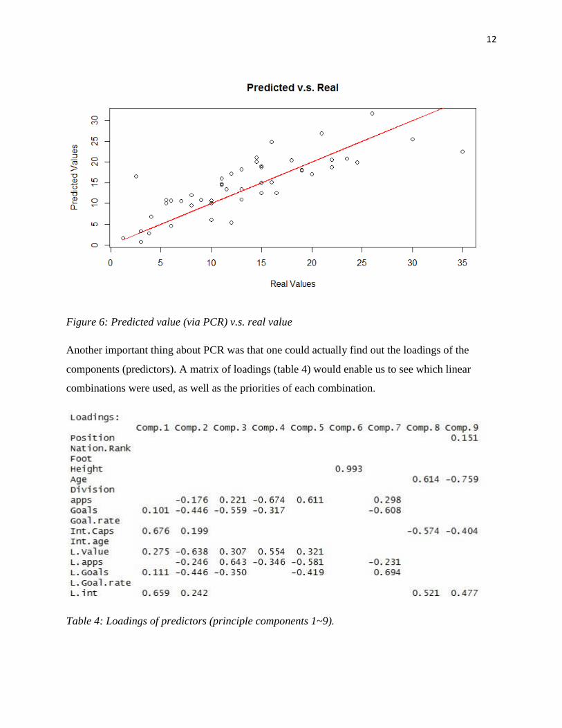
A visualization of the prediction by PCR (figure 6) showed that that the prediction was generally

accurate except for the lower tail. This was not surprising because players in their very early

years had no reputation and had values smaller than 1 million Euros. A boxplot would mark

these values as outliers. Therefore PCR tended to overestimate these small values from the lower

tail.

12

Figure 6: Predicted value (via PCR) v.s. real value

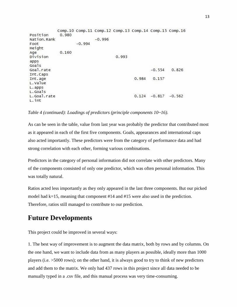
Another important thing about PCR was that one could actually find out the loadings of the

components (predictors). A matrix of loadings (table 4) would enable us to see which linear

combinations were used, as well as the priorities of each combination.

Table 4: Loadings of predictors (principle components 1~9).

13

Table 4 (continued): Loadings of predictors (principle components 10~16).

As can be seen in the table, value from last year was probably the predictor that contributed most

as it appeared in each of the first five components. Goals, appearances and international caps

also acted importantly. These predictors were from the category of performance data and had

strong correlation with each other, forming various combinations.

Predictors in the category of personal information did not correlate with other predictors. Many

of the components consisted of only one predictor, which was often personal information. This

was totally natural.

Ratios acted less importantly as they only appeared in the last three components. But our picked

model had k=15, meaning that component #14 and #15 were also used in the prediction.

Therefore, ratios still managed to contribute to our prediction.

Future Developments

This project could be improved in several ways:

1. The best way of improvement is to augment the data matrix, both by rows and by columns. On

the one hand, we want to include data from as many players as possible, ideally more than 1000

players (i.e. >5000 rows); on the other hand, it is always good to try to think of new predictors

and add them to the matrix. We only had 437 rows in this project since all data needed to be

manually typed in a .csv file, and this manual process was very time-consuming.

14

2. Our predictors did not cover every possible factor that could affect players' market value. For

example, major transfers and decisive performance in key games are both crucial to a player's

value. However, it was hard to convert these two factors into annual predictors and they were

thus missing from our data matrix.

3. Players from different positions should have different criteria for judging their performance.

For example, goals should be a fair assessment of a striker's ability, but not so fair for defenders

or goalkeepers. If we could include data such as number of assists, number of clean sheets,

tackles per game, etc., it would be much better for the evaluation of midfielders (assists),

defenders (tackles) and goalkeepers (clean sheets). Again this was not possible since detailed

performance data could only be found for current season.

Conclusion

In this project we built a data matrix consisting of independent variable (market value) and

dependent variables (predictors). Several modeling techniques were used to make predictions

and efficiency of each model was tested. With 16 predictors presented, PCR with k = 15 was the

model that performed best. In the final check of this model, it managed to yield more accurate

predictions than the natural predictor -- value from last year.

Visualization of the prediction showed that PCR tended to overestimate the lower tail. This was

acceptable given the context. A look at the loadings of principle components showed us the

weights and priorities of each predictor, as well as correlations between predictors. This project

highlights several factors that play an important role in players' market value, also figures out a

good model for making predictions based on these factors.

References

1. Lago, Carlos, and Rafael Martín. "Determinants of possession of the ball in soccer." Journal

of Sports Sciences 25, no. 9 (2007): 969-974.

2. Alex Ferguson, Paul Hayward. "Alex Ferguson--My Autobiography". Hodder & Stoughton

Press (2013).

15

3. Transfer Market website. http://www.transfermarkt.de/en.

4. Wikipedia. http://www.wikipedia.org.