Predicting Horizontal Gas Well Deliverability in a...
85
PREDICTING HORIZONTAL GAS WELL DELIVERABILITY IN A CONVENTIONAL RESERVOIR FROM VERTICAL WELL DATA Osade O. Edo-Osagie A Problem Report Submitted to the College of Engineering and Mineral Resources at West Virginia University In Partial Fulfillment of the Requirements of the degree of Master of Science In Petroleum and Natural Gas Engineering Khashayar Aminian, Ph.D. Samuel Ameri, M.S. Ilkin H. Bilgesu, Ph.D. Department of Petroleum and Natural Gas Engineering Morgantown, West Virginia 2011 Keywords: Horizontal Well, Vertical Well, Conventional Gas Reservoir, Deliverability, ECLIPSE Copyright 2011 Osade O. Edo-Osagie
Transcript of Predicting Horizontal Gas Well Deliverability in a...

PREDICTING HORIZONTAL GAS WELL DELIVERABILITY IN A CONVENTIONAL RESERVOIR FROM VERTICAL WELL DATA
Osade O. Edo-Osagie
A Problem Report Submitted to the
College of Engineering and Mineral Resources at
West Virginia University
In Partial Fulfillment of the Requirements of the degree of
Master of Science
In
Petroleum and Natural Gas Engineering
Khashayar Aminian, Ph.D.
Samuel Ameri, M.S.
Ilkin H. Bilgesu, Ph.D.
Department of Petroleum and Natural Gas Engineering
Morgantown, West Virginia
2011
Keywords: Horizontal Well, Vertical Well, Conventional Gas Reservoir, Deliverability, ECLIPSE
Copyright 2011 Osade O. Edo-Osagie

ABSTRACT
PREDICTING HORIZONTAL GAS WELL DELIVERABILITY IN A CONVENTIONAL RESERVOIR FROM
VERTICAL WELL DATA
Osade Edo-Osagie
This research project focuses on predicting the deliverability of horizontal gas wells in a
conventional reservoir based on well test data made available from the already existing vertical
wells. ECLIPSE reservoir simulation software by Schlumberger was employed for this research.
The first objective of the project was to obtain production results from ECLIPSE and compare
the results to the mathematical gas flow equations to check for validity and consistency. The
ultimate objective however was to determine how the deliverability constants (A and B values)
for the horizontal gas well are impacted by various reservoir parameters including well length,
drainage area, shape aspect ratio (xe/ye), permeability etc.
Using ECLIPSE completions tool template, production results were obtained. The deliverability
constants A and B were determined and different scenarios in terms of reservoir and well
parameters were taken into account. Monitoring the effects on deliverability was necessary in
achieving desired results.
Results were summarized in terms of the ratio of the horizontal to vertical deliverability
constants profile. Since the vertical deliverability is supposedly known and the horizontal to
vertical deliverability ratio profiles were obtained for each scenario, the horizontal deliverability
can be determined by identifying the case matching the particular situation.

iii
DEDICATION
I dedicate this paper first to my father Engr. Osato Edo-Osagie for ever willing support in
numerous forms all through my education, and then to my mother Mrs. Helen Edo-Osagie also
for her love, care and support, and finally to my siblings Osato Jr., Ifueko, Eseosa and Osaze
Edo-Osagie whom I’ve always seemed to lean on at one point or another.

iv
ACKNOWLEDGEMENT
I would like to thank God for his continued guidance. I would also express my gratitude to Dr.
Khashayar Aminian for his supervision throughout this research work and for being an excellent
advisor throughout my graduate studies at West Virginia University. Special thanks are also
directed to the rest of my graduate committee: Prof. Sam Ameri and Dr. Ilkin H. Bilgesu, for
their necessary input and overseeing of my research work.
Finally I would thank my colleagues and friends in the department of Petroleum and Natural
Gas Engineering, in the College of Engineering and Mineral Resources at the University and
everyone else that helped me even in the least amount during my research and graduate
studies here.

v
TABLE OF CONTENTS
ABSTRACT .........................................................................................................................................ii
DEDICATION .................................................................................................................................... iii
ACKNOWLEDGEMENT ..................................................................................................................... iv
TABLE OF CONTENTS........................................................................................................................ v
LIST OF FIGURES ............................................................................................................................. vii
LIST OF TABLES ................................................................................................................................ xi
CHAPTER 1....................................................................................................................................... 1
INTRODUCTION ............................................................................................................................... 1
CHAPTER 2....................................................................................................................................... 2
LITERATURE REVIEW ....................................................................................................................... 2
HORIZONTAL/MULTILATERAL WELLS ......................................................................................... 2
ECLIPSE ........................................................................................................................................ 3
GAS FLOW EQUATIONS ............................................................................................................... 4
DELIVERABILITY ........................................................................................................................... 9
CHAPTER 3..................................................................................................................................... 10
METHODOLOGY ............................................................................................................................ 10
REPRESENTATIVE DATA ............................................................................................................ 10
PRODUCTION ESTIMATION ....................................................................................................... 11
NON-DARCY INTEGRATION ....................................................................................................... 17
DELIVERABILITY CONSTANTS .................................................................................................... 19
PERFORMANCE PREDICTION .................................................................................................... 19
CHAPTER 4..................................................................................................................................... 20

vi
RESULTS AND DISCUSSIONS .......................................................................................................... 20
HORIZONTAL WELL LENGTH ..................................................................................................... 25
SHAPE ASPECT RATIO ................................................................................................................ 26
DRAINAGE AREA........................................................................................................................ 27
FORMATION HEIGHT ................................................................................................................. 29
RESERVOIR VERTICAL AND HORIZONTAL PERMEABILITY ......................................................... 30
DIMENSIONLESS WELL LENGTH ................................................................................................ 34
CHAPTER 5..................................................................................................................................... 44
SUMMARY AND CONCLUSIONS .................................................................................................... 44
APPENDIX ...................................................................................................................................... 45
APPENDIX A: USING GAS FLOW EQUATIONS ............................................................................ 45
APPENDIX B: USING ECLIPSE ..................................................................................................... 52
NOMENCLATURE ........................................................................................................................... 72
REFERENCES .................................................................................................................................. 74

vii
LIST OF FIGURES
Figure 3.1: Vertical well mathematical model ................................................................................ 5
Figure 3.2: Horizontal well mathematical model ........................................................................... 5
Figure 3.3: Shape related skin factor sCA,h, for a horizontal well in a rectangular drainage area
(xe/ye=2) .......................................................................................................................................... 8
Figure 3.4: ECLIPSE template model definition ............................................................................ 12
Figure 3.5: ECLIPSE template reservoir description ..................................................................... 12
Figure 3.6: ECLIPSE generated vertical well model ...................................................................... 13
Figure 3.7: ECLIPSE template well configuration .......................................................................... 14
Figure 3.8: ECLIPSE template production specification ................................................................ 14
Figure 3.9: ECLIPSE generated horizontal well model .................................................................. 15
Figure 3.10: Reservoir relative dimensions .................................................................................. 16
Figure 3.11: Vertical well grid allocation ...................................................................................... 16
Figure 3.12: Horizontal well grid allocation .................................................................................. 17
Figure 3.13: ECLIPSE data manager well completions specification ............................................ 18
Figure 4.1: IPR curve for reservoir pressure of 2000psia ............................................................. 21
Figure 4.2: IPR curve for reservoir pressure of 1800psia ............................................................. 21
Figure 4.3: IPR curve for reservoir pressure of 1600psia ............................................................. 22
Figure 4.4: IPR curve for reservoir pressure of 1400psia ............................................................. 22
Figure 4.5: AH/AV vs L/2xe .............................................................................................................. 25
Figure 4.6: AH/AV vs L/2xe at different area aspect ratios ............................................................. 26
Figure 4.7: AH/AV vs L/2xe at different area aspect ratios at twice the drainage area ................. 27
Figure 4.8: AH/AV vs L/2xe at xe/ye =1 for different drainage areas ............................................... 28

viii
Figure 4.9: AH/AV vs L/2xe at xe/ye =2 for different drainage areas ............................................... 28
Figure 4.10: AH/AV vs L/2xe at xe/ye =5 for different drainage areas ............................................. 29
Figure 4.11: AH/AV vs L/2xe at different reservoir thicknesses ...................................................... 30
Figure 4.12: AH/AV vs L/2xe at different reservoir thicknesses for kV/kH=1/10 ............................. 31
Figure 4.13: AH/AV vs L/2xe at different reservoir thicknesses for kV/kH=2/20 ............................. 31
Figure 4.14: AH/AV vs L/2xe at different reservoir thicknesses for kV/kH=2/10 ............................. 32
Figure 4.15: AH/AV vs L/2xe at 60ft reservoir thickness for at different kV/ kH ratios.................... 33
Figure 4.16: AH/AV vs L/2xe at 120ft reservoir thickness for at different kV/ kH ratios.................. 33
Figure 4.17: AH/AV vs L/2xe at 60ft reservoir thickness for at different kV/ kH ratios.................... 34
Figure 4.18: AH/AV vs L/2xe at different LD values for constant kV/ kH for xe/ye =1 ....................... 35
Figure 4.19: AH/AV vs L/2xe at different LD values for constant h for xe/ye =1 ............................... 35
Figure 4.20: AH/AV vs L/2xe at LD =1 for xe/ye =1 ........................................................................... 36
Figure 4.21: AH/AV vs L/2xe at LD =2 for xe/ye =1 ........................................................................... 36
Figure 4.22: AH/AV vs L/2xe at LD =3 for xe/ye =1 ........................................................................... 37
Figure 4.23: Average AH/AV vs L/2xe at LD =1 for xe/ye =1 ............................................................. 38
Figure 4.24: Average AH/AV vs L/2xe at LD =2 for xe/ye =1 ............................................................. 38
Figure 4.25: Average AH/AV vs L/2xe at LD =3 for xe/ye =1 ............................................................. 39
Figure 4.26: AH/AV vs L/2xe at different LD values for constant kV/ kH for xe/ye =2 ....................... 39
Figure 4.27: AH/AV vs L/2xe at different LD values for constant h for xe/ye =2 ............................... 40
Figure 4.28: AH/AV vs L/2xe at LD =1 for xe/ye =2 ........................................................................... 40
Figure 4.29: AH/AV vs L/2xe at LD =2 for xe/ye =2 ........................................................................... 41
Figure 4.30: AH/AV vs L/2xe at LD =3 for xe/ye =2 ........................................................................... 41
Figure 4.31: Average AH/AV vs L/2xe at LD =1 for xe/ye =2 ............................................................. 42
Figure 4.32: Average AH/AV vs L/2xe at LD =2 for xe/ye =2 ............................................................. 42

ix
Figure 4.33: Average AH/AV vs L/2xe at LD =3 for xe/ye =2 ............................................................. 43
Figure A.1: Shape related skin factor SCA,h, for horizontal well in a rectangular drainage area
(xe/ye=2) ....................................................................................................................................... 46
Figure A.2: Gas properties .exe program for computing μ and z ................................................. 47
Figure A.3: Shape related skin factor SCA,h, for horizontal well in a square drainage area
(xe/ye=1) ....................................................................................................................................... 49
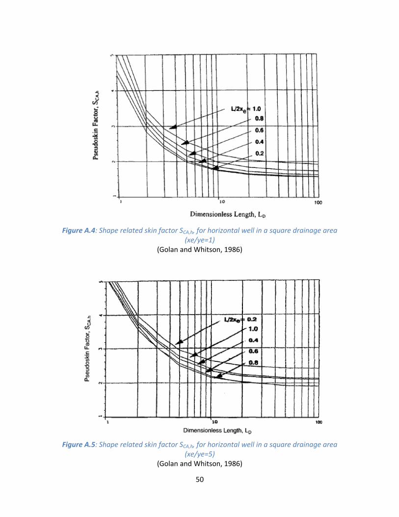
Figure A.4: Shape related skin factor SCA,h, for horizontal well in a square drainage area
(xe/ye=1) ....................................................................................................................................... 50
Figure A.5: Shape related skin factor SCA,h, for horizontal well in a square drainage area
(xe/ye=5) ....................................................................................................................................... 50
Figure B.1: Model Definition ........................................................................................................ 52
Figure B.2: Reservoir description (Layers) .................................................................................... 52
Figure B.3: Reservoir description (Rock properties) ..................................................................... 53
Figure B.4: Reservoir description (Initial conditions) ................................................................... 53
Figure B.5: Reservoir description (Aquifers) ................................................................................. 54
Figure B.6: Wells (Well deviation, vertical well) ........................................................................... 54
Figure B.7: Wells (Well deviation, 1st lateral) .............................................................................. 55
Figure B.8: Wells (Well deviation, 2nd lateral) ............................................................................. 55
Figure B.9: Wells (Casing) ............................................................................................................. 56
Figure B.10: Wells (Tubing) ........................................................................................................... 56
Figure B.11: Production ................................................................................................................ 57
Figure B.12: Fluid properties (PVT correlations) .......................................................................... 57
Figure B.13: Fluid properties (Advanced) ..................................................................................... 58
Figure B.14: Simulation controls (Gridding) ................................................................................. 58
Figure B.15: Simulation controls (Tuning) .................................................................................... 59

x
Figure B.16: Economics ................................................................................................................. 59
Figure B.17: Gas rate profile from ECLIPSE results ....................................................................... 60
Figure B.18: Field pressure profile from ECLIPSE results.............................................................. 61
Figure B.19: Bottomhole pressure profile from ECLIPSE results .................................................. 62
Figure B.20: Bottomhole pressure profile showing straight line decline ..................................... 63
Figure B.21: Field pressure profile showing selected point in the pseudosteady state period ... 64

xi
LIST OF TABLES
Table 3.1: Shape dependent skin factors, sCA, for vertical wells .................................................... 7
Table 3.2: Base case reservoir and wellbore parameters ............................................................ 11
Table 4.1: Vertical and horizontal well production rates at different conditions ........................ 20
Table 4.2: Relative percentage increases in production rate ....................................................... 23
Table 4.3: Vertical well sample runs at different rates and times ............................................... 24
Table 4.4: Corresponding horizontal well runs at the rates and times ........................................ 24
Table A.1: Shape dependent skin factors, sCA, for vertical wells .................................................. 51
Table B.1: Pressure and rate profiles for base case at xe/ye =1 with A values ............................. 65
Table B.2: AH/AV values for base case at different xe/ye values ................................................... 66
Table B.3: AH/AV values for 4000000ft drainage area .................................................................. 67
Table B.4.1: Total horizontal well skin factor for A=2000000ft2 .................................................. 67
Table B.4.2: Total horizontal well skin factor for A=4000000ft2 .................................................. 68
Table B.5: AH/AV values for different h values at kv/kh = 1/10 ..................................................... 68
Table B.6: AH/AV values for different h values at kv/kh = 2/20 ..................................................... 69
Table B.7: AH/AV values for different h values at kv/kh = 2/10 ..................................................... 69
Table B.8: AH/AV values for different LD values for xe/ye = 1 (kv/kh = constant) ........................... 70
Table B.9: AH/AV values for different LD values for xe/ye = 1 (h = constant) ................................. 70
Table B.10: AH/AV values for different LD values for xe/ye = 2 (kv/kh = constant) ......................... 71
Table B.11: AH/AV values for different LD values for xe/ye = 2 (h = constant) ............................... 71

1
CHAPTER 1
INTRODUCTION
Horizontal wells offer potential for increase in productivity, reduction of water or gas coning,
reduction of turbulence in gas wells, intersection of fractures in naturally fractured reservoirs
hence drain reservoirs more effectively, improvement in drainage area per well and hence
reduction in the number of vertical wells in low permeability reservoirs, increase in injectivity of
an injection well, enhancement of sweep efficiency, etc. Drilling horizontal wells instead of
vertical wells in hydrocarbon formations is therefore important because of many of these
advantages. It is however necessary to predict the performance of a horizontal well to
determine its economic feasibility. Currently, there is limited information on ways to compute
productivity, devise procedures that evaluate the completion efficiency, and predict
performance of the horizontal wells.
Previous studies have been conducted in the area of predicting horizontal well deliverability but
not in the attempt to predict it from that of a vertical well based on certain parameters in
conventional reservoirs. For example, Chase and Steffy (2004) published a paper on predicting
horizontal gas well deliverability using dimensionless IPR curves. Chen et al (2000) developed a
deliverability model to predict the performance of multilateral wells. Wang and Economides
(2009) predicted horizontal well deliverability with turbulence effects. This research, however,
tackles the aforementioned problem by dealing differently with comparing the deliverability of
a horizontal gas well with that of a vertical one for prediction purposes.
The main purpose of this research was to determine how the deliverability constants of a
horizontal gas well differed as compared to that of a vertical well with reservoir and well
parameters. The parameters taken into consideration were the horizontal well length,
reservoir drainage area, shape aspect ratio, formation height and permeability. The
dimensionless length (LD), a combination of certain parameters, which is explained later in this
paper, was also taken into account.
2
CHAPTER 2
LITERATURE REVIEW
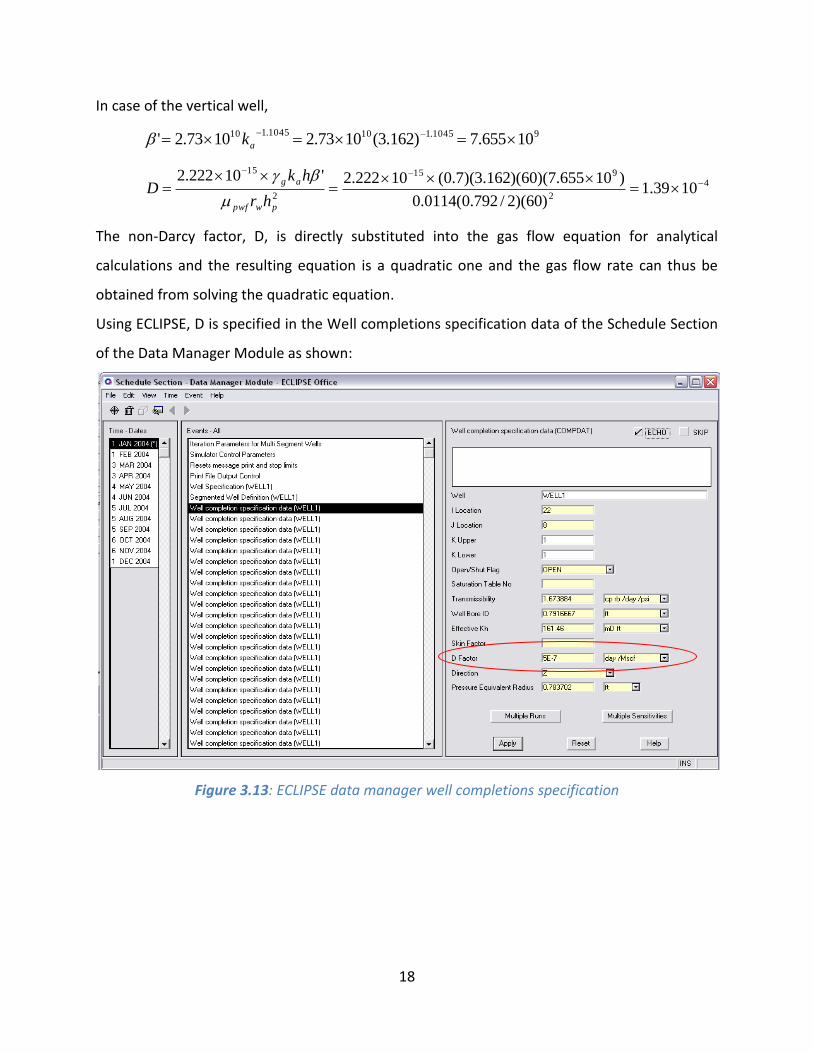
HORIZONTAL/MULTILATERAL WELLS
The drilling of horizontal wells started in the 1980s and became common in the early 1990s.
They have since then proliferated and become essential for today’s hydrocarbon production.
Advantages of drilling a horizontal well over a vertical well include to increase productivity,
reduce water or gas coning, reduce turbulence in gas wells, intersect fractures in naturally
fractured reservoirs hence drain reservoirs more effectively, improve drainage area per well
hence reducing the number of vertical wells in low permeability reservoirs, increase injectivity
of an injection well and enhance sweep efficiency.
Multilateral wells offer the potential for substantial improvement in well economics. In
multilateral well completions, two or more horizontal wellbores are drilled from a single parent
wellbore, enabling drainage of multiple reservoir targets. This technology allows the same
magnitude of reservoir exposure with a lesser number of wells on the surface/platform. The
benefits from multilateral well technology include increased production per platform slot,
exploitation of reservoirs with vertical permeability barriers, and production from natural
fracture systems, and others similar to those listed for horizontal wells. The modeling of
multilateral wells may be complicated for certain configurations because of the interplay
between reservoir performance and pressure loss in the wellbore. There have also been limited
information on ways to compute productivity, devise procedures that evaluate the completion
efficiency, and predict performance of the completion.
There are different methods that have been presented to determine productivity indices or skin
values for multilateral well systems.
For this research, horizontal wells were formed in each case from two laterals made from the
vertical well in the reservoir formation facing opposite directions (hence forming one longer
lateral or one horizontal well).

3
ECLIPSE
Reservoir simulation can be defined as an area of reservoir engineering in which computer
models are used to predict fluid flow in a porous media, in this case the reservoir, assumed to
mimic typical conditions. They can help in the development of new fields and can be analyzed
for production forecasts in order to help make important investment decisions. There are
numerous reservoir simulation software used today by professionals, some of which include
CMG, ECLIPSE, PETREL etc. to name a few. ECLIPSE (Office 2010) software by Schlumberger was
employed for this research.
ECLIPSE is an oil and gas reservoir simulator first developed by Exploration Consultants Limited
(ECL) but is currently owned, developed, marketed and maintained by SIS (formerly known as
GeoQuest), a division of Schlumberger. The name ECLIPSE was an acronym for "ECL´s Implicit
Program for Simulation Engineering". Ian Cheshire was one of the main engineers that
developed the program.
ECLIPSE uses the finite differences method to solve material and energy balance equations
modeling a subsurface petroleum reservoir. Versions include ECLIPSE 100 which solves the
black oil equations (a fluid model) on corner-point grids, ECLIPSE 300 that solves the reservoir
flow equations for compositional hydrocarbon descriptions and thermal simulation and
Intersect, a next generation reservoir simulator developed in partnership with Chevron.
ECLIPSE software covers a wide spectrum of reservoir simulation, specializing in blackoil,
compositional and thermal volume-difference reservoir simulation, and streamline reservoir
simulation. By choosing from a wide range of add-on options, like coalbed methane, gas field
operations, calorific value-based controls, reservoir coupling, and surface networks, simulator
capabilities can be tailored for different models, and can help enhance the scope of reservoir
simulation studies.

4
GAS FLOW EQUATIONS
The pseudo-steady state equation for a well on the basis of a rectangular drainage area is given as (Chaudhri, 2003):
gcAmwe
sc
scg
wfR DqcsssACrrkhT
TPzqpp
''ln
10335.50 3
22
where
2
15 '10222.2
pwpwf
ag
hr
kD
1045.1101073.2' ak
vha kkk
and
s => equivalent negative skin factor due to either well stimulation or horizontal well,
dimensionless
sm => mechanical skin factor, dimensionless
sCA => shape-related skin factor, dimensionless
c’ => shape factor conversion constant, dimensionless
k => permeability, millidarcy
h => reservoir height, feet
pR => average reservoir pressure, pounds per square inches
pwf => well flowing pressure, pounds per square inches
qg => gas flow rate, thousand standard cubic feet per day
T => reservoir temperature, Rankin
µ => gas viscosity at well flowing conditions, centipoise
z => gas compressibility factor evaluated at some average pressure between pR and
pwf, dimensionless
β’ => high velocity flow coefficient, per foot
g => gas gravity, dimensionless
rw => wellbore radius, feet

5
hp => perforated interval, feet
ka => permeability in near wellbore region, millidarcy
AC’ => 0.738 for a rectangular drainage area, dimensionless
In order to calculate gas flow rate, the above equation can be rewritten as:
gCAmwesc
wfRsc
gDqcsssrrTPz
ppkhTq
'738.0ln
10019866.0 226
The mathematical model for the vertical well is shown in figure 3.1.
Figure 3.1: Vertical well mathematical model
The mathematical model for the horizontal well is shown in figure 3.2.
Figure 3.2: Horizontal well mathematical model
Also note that:
2, ftArev
evrLa 2/'
a’
2xe
b’ L
2ye
2xe

6
evrb '
ftrrLr eveveh ,2/
5.0
5.04
/225.05.02/
LrL eh
5.0
vh kk
4
' Lrw
0'c for vertical gas wells
386.1'c for horizontal gas wells
0s for vertical gas wells (no stimulation)
ww rrs /ln '
for horizontal gas wells
h
vD
k
k
h
LL
2
sCA is obtained from charts:
For a vertical well, sCA is obtained from table 3.1.

7
Table 3.1: Shape dependent skin factors, sCA, for vertical wells (Fetkovich and Vienot, 1985)
For a horizontal well, sCA is obtained from using LD and 2xe values for the sCA,h charts. An
example is illustrated in figure 3.3.

8
Figure 3.3: Shape related skin factor sCA,h, for a horizontal well in a rectangular drainage area (xe/ye=2)
(Golan and Whitson, 1986)
Mechanical skin, sm, is assumed to be negligible
For a vertical gas well therefore, the flow equation becomes:
gCAwesc
wfRsc
gDqsrrTPz
ppkhTq
738.0ln
10019866.0 226
………………………….................................2.1
And for a horizontal gas well, the flow equation becomes:
gCAwesc
wfRsc
gDqssrrTPz
ppkhTq
386.1738.0ln
10019866.0 226
………………………………………2.2
Production rate values are obtained by substituting for the parameters remaining, the values
aforementioned previously in the data section.
(D = 0 for calculations without non-Darcy or turbulence effect)

9
DELIVERABILITY
The constants A and B can be determined from flow tests for at least two rates in which the
flow rate, qsc, and corresponding well-flowing or bottom-hole pressure, pwf, values are
measured; reservoir pressure, pR, also must be known. A is usually referred to as the laminar
constant while B is referred to as the turbulence constant.
gcAmwe
sc
scg
scscwfRDqcsssACrr
khT
TPzqBqAqpp
''ln
10335.50 3
222
(Chaudhri, 2003)
Using the gas flow equations for a horizontal well therefore,
'738.0ln1422'738.0ln
10337.50 3
cssr
r
kh
Tzcss
r
r
khT
TpzA cA
w
ecA
w
e
sc
sc
HH
sc
sc Dkh
TzD
khT
TpzB
1422
10337.50 3
……………………………………………………………….2.3
Or for a vertical well,
cA
w
ecA
w
e
sc
sc sr
r
kh
Tzs
r
r
khT
TpzA 738.0ln1422738.0ln
10337.50 3
VV
sc
sc Dkh
TzD
khT
TpzB
1422
10337.50 3
……………………………………………………………….2.4

10
CHAPTER 3
METHODOLOGY
It is important to note that for this research, synthetic data which fall within real average limits
have been employed as the sample data for the use as the base case and the results obtained
are relative to the various syntactic situations which were predefined.
The methodology to achieve the results included the following steps:
- Obtaining production results from gas flow equations and from ECLIPSE simulation runs
for the vertical and horizontal wells during pseudosteady state period and then
comparing both to check for consistency and validity.
- Integrating non-Darcy (turbulence) into both methods and analyze similarly accordingly.
- Deriving deliverability constants A and B for both vertical and horizontal wells using the
analytical and simulation approach and testing for validity and consistency.
- Finally determining how the constants A and B vary with respect to change in the
following parameters:
o Horizontal well length
o Reservoir drainage area
o Shape aspect ratio
o Reservoir vertical and horizontal permeability
o Formation height
o Dimensionless horizontal well length
REPRESENTATIVE DATA
Unless otherwise indicated, the reservoir and wellbore parameters were used for the base case
for the project are shown in table 3.2.

11
Table 3.2: Base case reservoir and wellbore parameters
PRODUCTION ESTIMATION
Production information was obtained in two ways:
- Using the pseudo-steady state gas flow mathematical equations.
- Using ECLIPSE software (completions tool template).
Pseudo-Steady State Gas Flow Mathematical Equations:
The gas flow equations used for the wells have been illustrated in the previous section.
Equation 2.1 shows the general equation used in the case of a vertical well while equation 2.2
shows the general equation used in the case of a horizontal well.
Parameter Value Unit
Initial reservoir pressure 2000 psia
Well flowing pressure 500 psia
Reservoir temperature 110 °F
Standard conditions pressure 14.7 psia
Standard conditions temperature 520 R
Horizontal permeability 10 md
Vertical permeability 1 md
Drainage area 2000000 ft2
Shape aspect ratio (xe/ye) 2
Reservoir thickness 60 ft
Horizontal well length 1000 ft
Hole diameter 9.5 in
Reservoir true vertical depth 5000 ft
Porosity 0.1
Gas gravity 0.7

12
Production using ECLIPSE:
Results were obtained using the completions tool model template. The model was defined as a
dry gas model with simulation length and reporting of about 1 year. The reservoir was
described according to the parameters previously mentioned in the data section. Figures 3.4
and 3.5 show some of the model input templates.
Figure 3.4: ECLIPSE template model definition
Figure 3.5: ECLIPSE template reservoir description

13
For vertical well production, a vertical well was created down through the formation and
perforated from the producing reservoir’s top to bottom depth. The vertical well model is
illustrated as follows:
Figure 3.6: ECLIPSE generated vertical well model
For horizontal well production, two equidistant laterals of the same length each were made
from the vertical well in the middle of the reservoir facing opposite directions (hence a
combined horizontal well of length twice the length of one of the laterals). Production was
obtained from the well while only the laterals were perforated.

14
Figure 3.7: ECLIPSE template well configuration
Figure 3.8: ECLIPSE template production specification

15
The horizontal well model generated is illustrated as follows:
Figure 3.9: ECLIPSE generated horizontal well model
The reservoir was rendered transparent in order to show the two laterals from “Well1” forming
the horizontal well. The relative reservoir dimensions can be seen on the next illustration.

16
Figure 3.10: Reservoir relative dimensions
After inputting all the necessary parameters, the simulation was run and results were obtained.
Figure 3.11: Vertical well grid allocation

17
Figure 3.12: Horizontal well grid allocation
NON-DARCY INTEGRATION
Calculation of D-factor:
2
15 '10222.2
pwpwf
ag
hr
kD
1045.1101073.2' ak
vha kkk
For a vertical well, the perforated interval is the height of the formation while the length of the
well is regarded as the perforation interval for a horizontal well.
For the base case of the horizontal well for example,
91045.1101045.110 10655.7)162.3(1073.21073.2'
ak
7
2
915
2
15
1000.5)1000)(2/792.0(0114.0
)10655.7)(60)(162.3)(7.0(10222.2'10222.2
pwpwf
ag
hr
hkD
18
In case of the vertical well,
91045.1101045.110 10655.7)162.3(1073.21073.2'
ak
4
2
915
2
15
1039.1)60)(2/792.0(0114.0
)10655.7)(60)(162.3)(7.0(10222.2'10222.2
pwpwf
ag
hr
hkD
The non-Darcy factor, D, is directly substituted into the gas flow equation for analytical
calculations and the resulting equation is a quadratic one and the gas flow rate can thus be
obtained from solving the quadratic equation.
Using ECLIPSE, D is specified in the Well completions specification data of the Schedule Section
of the Data Manager Module as shown:
Figure 3.13: ECLIPSE data manager well completions specification

19
DELIVERABILITY CONSTANTS
Obtaining the deliverability constants A and B from the gas flow equations have been illustrated
in the previous section. Equation 2.4 shows the general equation used in the case of a vertical
well while equation 2.3 shows the general equation used in the case of a horizontal well.
Determining the constants from ECLIPSE simulation involved obtaining the reservoir and
bottomhole pressure profiles and relative production values. A and B values were derived
during pseudosteady state accordingly.
sc
wfR
q
ppA
22
…….from simulation without non-Darcy integration
Then 2
22
sc
scwfR
q
AqppB
……..from simulation with non-Darcy integration
PERFORMANCE PREDICTION
The results obtained from following the methodology described above were compared and
checked for validity and consistency. After that task was completed, vital analysis was
performed using the ECLIPSE reservoir simulation software. Variations in the values of
constants A and B with respect to change in horizontal well length, reservoir drainage area,
drainage area aspect ratio, reservoir vertical and horizontal permeability, formation height and
finally dimensionless horizontal well length, which is a combination of the well length,
formation height and ratio of vertical to horizontal permeability, are derived for horizontal
wells as compared to vertical wells. Results for each case show a horizontal to vertical
deliverability constant ratio profiles. Since the vertical deliverability is supposedly known and
the horizontal to vertical deliverability ratio profiles were obtained for each case, the horizontal
deliverability can be determined by identifying the case matching the particular.

20
CHAPTER 4
RESULTS AND DISCUSSIONS
Using the pseudo-steady state gas flow rate mathematical equations to obtain production
information, the base case reservoir and wellbore parameters were employed in the necessary
equations to obtain production values for both vertical and horizontal wells. Note that this
result was obtained at different reservoir and bottom hole pressures. Refer to appendix A for
gas flow equations calculations.
Based on the parameters specified, the production rate for vertical and horizontal wells at
different reservoir and bottomhole pressure is summarized in Table 4.1.
Notice that the vertical well is significantly affected by the non-Darcy term but the horizontal
well is relatively unaffected in terms of production as seen in the 1000ft long case.
Table 4.1: Vertical and horizontal well production rates at different conditions
PR
BHP q BHP q BHP q BHP q BHP q BHP q
400 24436.58 400 36201.29865 400 147041.6 400 141279.7286 400 225726.4 400 285753.9
600 23569.9 600 34143.89758 600 138684.9 600 133698.7578 600 212897.9 600 269513.8
800 22177.67 800 31232.44576 800 126859.3 800 122790.2883 800 194744.1 800 246532.4
1000 20148.62 1000 27272.00854 1000 110772.9 1000 107783.1858 1000 170049.5 1000 215270.8
1200 17511.63 1200 22651.52425 1200 92005.47 1200 90012.22987 1200 141239.3 1200 178799.1
BHP q BHP q BHP q BHP q BHP q BHP q
400 20813.26 400 29347.82707 400 119204.4 400 115360.8923 400 182992.9 400 231656.2
600 19736.66 600 27150.97399 600 110281.2 600 107081.0183 600 169294.8 600 214315.4
800 18254.14 800 24388.49827 800 99060.67 800 96543.56903 800 152069.9 800 192509.9
1000 16210.63 1000 20821.6305 1000 84572.85 1000 82806.62941 1000 129829.4 1000 164354.9
1200 13367.97 1200 16363.20513 1200 66463.71 1200 65409.67751 1200 102029.7 1200 129162.5
BHP q BHP q BHP q BHP q BHP q BHP q
400 17259.89 400 23129.0696 400 93945.15 400 91524.33192 400 144217 400 182568.6
600 16055.96 600 20962.73362 600 85145.98 600 83211.90423 600 130709.2 600 165468.7
800 14323.61 800 18100.64933 800 73520.82 800 72114.86186 800 112863.2 800 142876.9
1000 12074.78 1000 14633.09896 1000 59436.4 1000 58551.90331 1000 91241.95 1000 115505.9
1200 9040.826 1200 10410.81525 1200 42286.42 1200 41853.61248 1200 64914.69 1200 82177.45
BHP q BHP q BHP q BHP q BHP q BHP q
400 13802.99 400 17556.57748 400 71310.92 400 69897.61589 400 109470.8 400 138582.3
600 12462.96 600 15419.37973 600 62630.1 600 61569.9074 600 96144.66 600 121712.4
800 10534.58 800 12577.64017 800 51087.59 800 50399.60352 800 78425.52 800 99281.22
1000 7943.22 1000 9050.324663 1000 36760.41 1000 36417.10725 1000 56431.61 1000 71438.46
1200 4533.254 1200 4877.699654 1200 19812.13 1200 19715.22943 1200 30413.98 1200 38501.97
1000' long Horizontal
Well (w/ Non-Darcy)
1500' long
Horizontal Well
2000ft long
Horizontal Well
1600
1400
Vertical Well (With
Non-Darcy)
1000' long
Horizontal Well
2000
1800
Vertical Well (Without
Non-Darcy)

21
The following IPR curves are generated from the results above:
Figure 4.1: IPR curve for reservoir pressure of 2000psia
Figure 4.2: IPR curve for reservoir pressure of 1800psia
0
50000
100000
150000
200000
250000
300000
350000
0 200 400 600 800 1000 1200 1400
q, m
scfd
BHP, psia
Pr = 2000psia
1000' HW
1500' HW
2000' HW
VW W/ ND
VW w/o ND
0
50000
100000
150000
200000
250000
0 200 400 600 800 1000 1200 1400
q, m
scfd
BHP, psia
Pr = 1800psia
1000' HW
1500' HW
2000' HW
VW w/ ND
VW w/o ND

22
Figure 4.3: IPR curve for reservoir pressure of 1600psia
Figure 4.4: IPR curve for reservoir pressure of 1400psia
0
20000
40000
60000
80000
100000
120000
140000
160000
180000
200000
0 200 400 600 800 1000 1200 1400
q, m
scfd
BHP, psia
Pr = 1600psia
1000' HW
1500' HW
2000' HW
VW w/ ND
VW w/o ND
0
20000
40000
60000
80000
100000
120000
140000
160000
0 200 400 600 800 1000 1200 1400
q, m
scfd
BHP, psia
Pr = 1400psia
1000' HW
1500' HW
2000' HW
VW w/ ND
VW w/o ND

23
Here is a table that shows the relative percentage increases in production rate:
Table 4.2: Relative percentage increases in production rate
Since this is a comparative analysis, a known value of production rate was directly employed in
the program as the constant well control property, while the bottomhole pressure (well flowing
pressure) was varied accordingly. This enables the procurement of a bottom hole pressure
profile (pressure versus time). The pseudo-steady state zone was identified from this profile as
evident by a constant change in pressure (straight line decline). A bottom hole pressure was
obtained at a particular time from within the pseudo-steady state zone. The corresponding
reservoir pressure at that same time was noted from the reservoir pressure profile. These
values of reservoir pressure and well flowing pressure were employed back into the gas flow
rate equations and a value of production, in thousand standard cubic feet per day, was
obtained and compared to the original value obtained initially from the pseudo-steady state gas
flow rate equations.
An alternative method employed was keeping the bottomhole pressure constant as the well
control property of the reservoir model and running simulations to obtain reservoir and
bottomhole pressure, and production profiles. Identifying a particular time during the
pseudosteady state region, the pressure values were employed into the gas flow equation and
PR VW w/ ND VW w/o ND 1000' HW 1500' HW 2000' HW
2000 0 40.828346 472.0135 778.1088 1011.624
1800 0 33.605267 442.675 733.0706 954.6091
1600 0 26.3692922 413.284 687.9521 897.4922
1400 0 19.3938134 384.9512 644.4578 842.4314
Average percentage increase in q over vertical well (with non-darcy effects):
PR VW w/ ND VW w/o ND 1000' HW 1500' HW 2000' HW
2000 110.52253 148.317215 148.3172 148.3172 148.3172
1800 73.278284 93.9036094 93.90361 93.90361 93.90361
1600 35.967546 43.9113305 43.91133 43.91133 43.91133
1400 0 0 0 0 0
Avg increase over 1400 psia PR:

24
a production rate value is obtained. Values are compared for validity. Different scenarios were
tried out to test for consistency.
Deliverability constants A and B values were determined and compared in a similar fashion
following the predefined equations shown in the methodology section. Note that B values were
negligible for horizontal wells as compared to that of vertical wells so focus was shifted to only
the deliverability constant A values for the remainder of this research work.
It was discovered at the end of the analysis that the values obtained using the gas flow
equations were very close to those obtained from ECLIPSE simulation runs with a percentage
error of about 6% or less. Refer to appendix B for ECLIPSE calculations and simulation run
results. The following tables show deliverability constant A values of sample runs at different
rates and times for a vertical well and corresponding horizontal well. Notice how the ratio of
horizontal to vertical A value is constant at 0.32.
Table 4.3: Vertical well sample runs at different rates and times
Table 4.4: Corresponding horizontal well runs at the rates and times
Thus illustrated are the variations in the values of the deliverability constant with respect to
change in the different factors. Starting from the base case scenario, all other factors except
t, days q, mscf/d pR, psia pwf, psia A=(pR^2-pwf^2)/q
600 1000 1781.4 1736.7 157
600 2000 1564.1 1467.2 147
400 3000 1561.3 1414.9 145
400 4000 1414.6 1199.4 140
200 5000 1641.4 1402.9 145
200 6000 1569.9 1269.1 142
t, days q, mscf/d pR, psia pwf, psia A=(pR^2-pwf^2)/q
600 1000 1781.4 1766.7 52
600 2000 1564.1 1533.4 48
400 3000 1561.3 1515.7 47
400 4000 1414.6 1349.3 45
200 5000 1641.4 1568.6 47
200 6000 1570 1480 46

25
that in consideration remain constant unless otherwise specified. In all cases, the horizontal
well is aligned in the x-direction in the middle of the producing reservoir.
HORIZONTAL WELL LENGTH
As previously seen, an increase in the length of a horizontal well increases the production rate
of the well (thereby decreasing the value of the deliverability constant A). In considering the
horizontal well length, the ratio of L/2xe is taken into account. The variation is illustrated in the
following chart, with AH/AV referring to the ratio of horizontal to vertical deliverability constant
A value.
Figure 4.5: AH/AV vs L/2xe
Note that a vertical well will result from a horizontal well length of 0ft, making the ratio AH/AV
equal to 1. The decline in that ratio can be seen in figure 4.5. L/2xe is used as the variable axis
for the rest of the analysis.
0
0.05
0.1
0.15
0.2
0.25
0.3
0.35
0.4
0.45
0.5
0 0.1 0.2 0.3 0.4 0.5 0.6 0.7 0.8
AH/A
V
L/2xe

26
SHAPE ASPECT RATIO
Next, the ratio is investigated for the change in the reservoir shape aspect ratio, xe/ye, which is
basically the ratio of the length to the breadth of the reservoir. Refer to figure 4.6 for the
resulting profile.
Figure 4.6: AH/AV vs L/2xe at different area aspect ratios
The aspect ratio definitely does impact the deliverability constant A value as shown in the chart
above. The trend shows less change however with further increase in the value of this aspect
ratio.
0
0.1
0.2
0.3
0.4
0.5
0.6
0 0.1 0.2 0.3 0.4 0.5 0.6 0.7 0.8
AH/A
V
L/2Xe
Xe/Ye=1
Xe/Ye=2
Xe/Ye=5

27
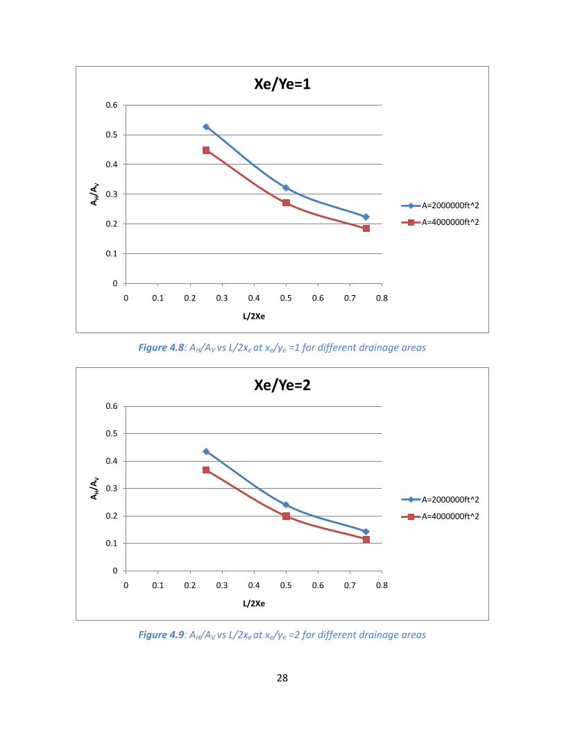
DRAINAGE AREA
Doubling the drainage area affects the ratio AH/AV. The profiles may look similar but the value
does drop indicating that the production is increased more so in the horizontal case than in the
vertical.
Figure 4.7: AH/AV vs L/2xe at different area aspect ratios at twice the drainage area
Figures 4.8, 4.9 and 4.10 show individual comparisons for each aspect ratio.
0
0.05
0.1
0.15
0.2
0.25
0.3
0.35
0.4
0.45
0.5
0 0.1 0.2 0.3 0.4 0.5 0.6 0.7 0.8
AH/A
V
L/2Xe
A=4000000sqft
Xe/Ye=1
Xe/Ye=2
Xe/Ye=5
28
Figure 4.8: AH/AV vs L/2xe at xe/ye =1 for different drainage areas
Figure 4.9: AH/AV vs L/2xe at xe/ye =2 for different drainage areas
0
0.1
0.2
0.3
0.4
0.5
0.6
0 0.1 0.2 0.3 0.4 0.5 0.6 0.7 0.8
AH/A
V
L/2Xe
Xe/Ye=1
A=2000000ft^2
A=4000000ft^2
0
0.1
0.2
0.3
0.4
0.5
0.6
0 0.1 0.2 0.3 0.4 0.5 0.6 0.7 0.8
AH/A
V
L/2Xe
Xe/Ye=2
A=2000000ft^2
A=4000000ft^2

29
Figure 4.10: AH/AV vs L/2xe at xe/ye =5 for different drainage areas
The trends show somewhat less difference in the AH/AV ratios with increasing well length and
aspect ratio.
FORMATION HEIGHT
Investigating the effect of the formation height on the deliverability constant, we realize the
profile illustrated in figure 4.11.
0
0.1
0.2
0.3
0.4
0.5
0.6
0 0.1 0.2 0.3 0.4 0.5 0.6 0.7 0.8
AH/A
V
L/2Xe
Xe/Ye=5
A=2000000ft^2
A=4000000ft^2

30
Figure 4.11: AH/AV vs L/2xe at different reservoir thicknesses
Remember that all other factors remain constant according to the base case described earlier
except that in consideration, in this case of which is the height of the formation. The trend
shows an increase in the ratio of AH to AV with increasing formation height meaning that the
horizontal well produces less in comparison with the vertical well with greater formation
heights. The difference is somewhat less pronounced with increasing well lengths.
RESERVOIR VERTICAL AND HORIZONTAL PERMEABILITY
In considering permeability, the ratio of vertical to horizontal permeability kV/kH is taken into
account. From the illustration seen in figures 4.12 and 4.13, changing the value of kV or kH has
no effect on the ratio AH/AV if kV/kH remains constant. The reservoir is considered to be
isotropic, meaning that kx = ky = kH, and kz = kV.
0
0.1
0.2
0.3
0.4
0.5
0.6
0.7
0 0.1 0.2 0.3 0.4 0.5 0.6 0.7 0.8
AH/A
V
L/2Xe
h=60
h=100
h=120

31
Figure 4.12: AH/AV vs L/2xe at different reservoir thicknesses for kV/kH=1/10
Figure 4.13: AH/AV vs L/2xe at different reservoir thicknesses for kV/kH=2/20
0
0.1
0.2
0.3
0.4
0.5
0.6
0.7
0 0.1 0.2 0.3 0.4 0.5 0.6 0.7 0.8
AH/A
V
L/2Xe
KV/kH = 1/10
h=60
h=100
h=120
0
0.1
0.2
0.3
0.4
0.5
0.6
0.7
0 0.1 0.2 0.3 0.4 0.5 0.6 0.7 0.8
AH/A
V
L/2Xe
KV/kH =2/20
h=60
h=100
h=120

32
However, a difference in profile is seen as the ratio of kV to kH changes. An increase in KV/kH
leads to a decrease in AH/AV, less pronounced in thinner formations. Figure 4.14 shows the
relationship involved when the ratio KV/kH is doubled.
Figure 4.14: AH/AV vs L/2xe at different reservoir thicknesses for kV/kH=2/10
Figures 4.15, 4.16 and 4.17 directly compare the ratios individually for the different reservoir
thicknesses. It can be seen how much the decrease in AH/AV is less pronounced in thinner
formations.
0
0.1
0.2
0.3
0.4
0.5
0.6
0 0.1 0.2 0.3 0.4 0.5 0.6 0.7 0.8
AH/A
V
L/2Xe
KV/kH = 2/10
h=60
h=100
h=120

33
Figure 4.15: AH/AV vs L/2xe at 60ft reservoir thickness for at different kV/ kH ratios
Figure 4.16: AH/AV vs L/2xe at 120ft reservoir thickness for at different kV/ kH ratios
0
0.1
0.2
0.3
0.4
0.5
0.6
0.7
0 0.1 0.2 0.3 0.4 0.5 0.6 0.7 0.8
AH/A
V
L/2Xe
h=60ft
kV/kH=0.1
kV/kH=0.2
0
0.1
0.2
0.3
0.4
0.5
0.6
0.7
0 0.1 0.2 0.3 0.4 0.5 0.6 0.7 0.8
AH/A
V
L/2Xe
h=100ft
kV/kH=0.1
kV/kH=0.2
34
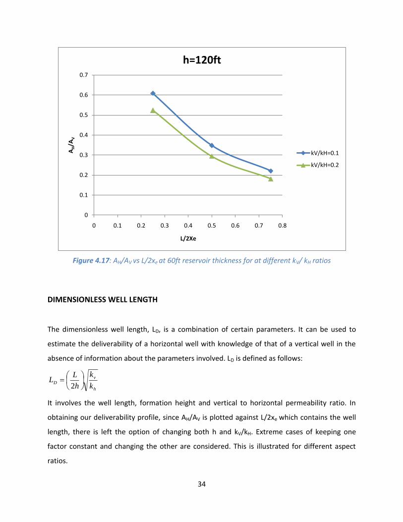
Figure 4.17: AH/AV vs L/2xe at 60ft reservoir thickness for at different kV/ kH ratios
DIMENSIONLESS WELL LENGTH
The dimensionless well length, LD, is a combination of certain parameters. It can be used to
estimate the deliverability of a horizontal well with knowledge of that of a vertical well in the
absence of information about the parameters involved. LD is defined as follows:
h
vD
k
k
h
LL
2
It involves the well length, formation height and vertical to horizontal permeability ratio. In
obtaining our deliverability profile, since AH/AV is plotted against L/2xe which contains the well
length, there is left the option of changing both h and kV/kH. Extreme cases of keeping one
factor constant and changing the other are considered. This is illustrated for different aspect
ratios.
0
0.1
0.2
0.3
0.4
0.5
0.6
0.7
0 0.1 0.2 0.3 0.4 0.5 0.6 0.7 0.8
AH/A
V
L/2Xe
h=120ft
kV/kH=0.1
kV/kH=0.2

35
For xe/ye = 1, keeping kV/kH constant (at 0.1) yields figure 4.18.
Figure 4.18: AH/AV vs L/2xe at different LD values for constant kV/ kH for xe/ye =1 Whereas keeping h constant (at 60ft) yields figure 4.19.
Figure 4.19: AH/AV vs L/2xe at different LD values for constant h for xe/ye =1
0
0.1
0.2
0.3
0.4
0.5
0.6
0 0.1 0.2 0.3 0.4 0.5 0.6 0.7 0.8
AH/A
V
L/2Xe
LD=1
LD=2
LD=3
0
0.1
0.2
0.3
0.4
0.5
0.6
0 0.1 0.2 0.3 0.4 0.5 0.6 0.7 0.8
AH/A
V
L/2Xe
LD=1
LD=2
LD=3

36
Analyzing both by comparing and contrasting gives figures 4.20, 4.21 and 4.22.
Figure 4.20: AH/AV vs L/2xe at LD =1 for xe/ye =1
Figure 4.21: AH/AV vs L/2xe at LD =2 for xe/ye =1
0
0.1
0.2
0.3
0.4
0.5
0.6
0 0.2 0.4 0.6 0.8
AH/A
V
L/2Xe
LD=1
h=cons
kV/kH=cons
0
0.1
0.2
0.3
0.4
0.5
0.6
0 0.2 0.4 0.6 0.8
AH/A
V
L/2Xe
LD=2
h=cons
kV/kH=cons

37
Figure 4.22: AH/AV vs L/2xe at LD =3 for xe/ye =1
Smaller LD values show relatively more scattered trends. General trends can be estimated by
taking the average of both curves in each case as shown in figures 4.23, 4.24 and 4.25.
0
0.1
0.2
0.3
0.4
0.5
0.6
0 0.1 0.2 0.3 0.4 0.5 0.6 0.7 0.8
AH/A
V
L/2Xe
LD=3
h=cons
kV/kH=cons
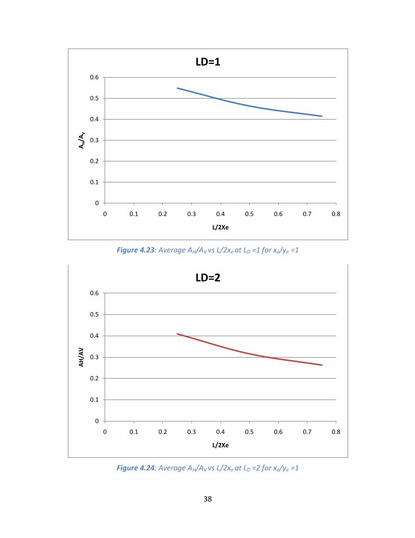
38
Figure 4.23: Average AH/AV vs L/2xe at LD =1 for xe/ye =1
Figure 4.24: Average AH/AV vs L/2xe at LD =2 for xe/ye =1
0
0.1
0.2
0.3
0.4
0.5
0.6
0 0.1 0.2 0.3 0.4 0.5 0.6 0.7 0.8
AH/A
V
L/2Xe
LD=1
0
0.1
0.2
0.3
0.4
0.5
0.6
0 0.1 0.2 0.3 0.4 0.5 0.6 0.7 0.8
AH
/AV
L/2Xe
LD=2

39
Figure 4.25: Average AH/AV vs L/2xe at LD =3 for xe/ye =1
For xe/ye = 2, keeping kV/kH constant (at 0.1) yields figure 4.26.
Figure 4.26: AH/AV vs L/2xe at different LD values for constant kV/ kH for xe/ye =2
0
0.1
0.2
0.3
0.4
0.5
0.6
0 0.1 0.2 0.3 0.4 0.5 0.6 0.7 0.8
AH
/AV
L/2Xe
LD=3
0
0.1
0.2
0.3
0.4
0.5
0.6
0 0.1 0.2 0.3 0.4 0.5 0.6 0.7 0.8
AH/A
V
L/2Xe
LD=1
LD=2
LD=3

40
Whereas keeping h constant yields figure 4.27.
Figure 4.27: AH/AV vs L/2xe at different LD values for constant h for xe/ye =2
Analyzing by comparing both ends with profiles shown in figures 4.28, 4.29 and 4.30.
Figure 4.28: AH/AV vs L/2xe at LD =1 for xe/ye =2
0
0.1
0.2
0.3
0.4
0.5
0.6
0 0.1 0.2 0.3 0.4 0.5 0.6 0.7 0.8
AH/A
V
L/2Xe
LD=1
LD=2
LD=3
0
0.1
0.2
0.3
0.4
0.5
0.6
0 0.2 0.4 0.6 0.8
AH/A
V
L/2Xe
LD=1
h=cons
kV/kH=cons

41
Figure 4.29: AH/AV vs L/2xe at LD =2 for xe/ye =2
Figure 4.30: AH/AV vs L/2xe at LD =3 for xe/ye =2
0
0.1
0.2
0.3
0.4
0.5
0.6
0 0.2 0.4 0.6 0.8
AH/A
V
L/2Xe
LD=2
h=cons
kV/kH=cons
0
0.1
0.2
0.3
0.4
0.5
0.6
0 0.2 0.4 0.6 0.8
AH/A
V
L/2Xe
LD=3
h=cons
kV/kH=cons

42
General trends can be estimated by taking the average of both curves in each case as shown in
figures 4.31, 4.32 and 4.33.
Figure 4.31: Average AH/AV vs L/2xe at LD =1 for xe/ye =2
Figure 4.32: Average AH/AV vs L/2xe at LD =2 for xe/ye =2
0
0.1
0.2
0.3
0.4
0.5
0.6
0 0.1 0.2 0.3 0.4 0.5 0.6 0.7 0.8
AH/A
V
L/2Xe
LD=1
0
0.1
0.2
0.3
0.4
0.5
0.6
0 0.1 0.2 0.3 0.4 0.5 0.6 0.7 0.8
AH/A
V
L/2Xe
LD=2

43
Figure 4.33: Average AH/AV vs L/2xe at LD =3 for xe/ye =2
0
0.1
0.2
0.3
0.4
0.5
0.6
0 0.1 0.2 0.3 0.4 0.5 0.6 0.7 0.8
AH/A
V
L/2Xe
LD=3

44
CHAPTER 5
SUMMARY AND CONCLUSIONS
The main purpose of this research was to determine how the deliverability constants of a
horizontal gas well differed as compared to that of a vertical well with reservoir and well
parameters. The parameters taken into consideration were the horizontal well length,
reservoir drainage area, area aspect ratio, formation height and permeability. The
dimensionless length (LD), a combination of the permeability ratio, reservoir thickness and well
length was also considered.
This study has showed that given the known deliverability of a vertical well, the deliverability of
a horizontal well producing in a similar reservoir can be estimated. Horizontal well deliverability
can be determined with availability of information on some of the different individual
parameters such as well length, shape aspect ratio, drainage area, formation height or
formation permeability, or collective parameters as seen in the case of the dimensionless well
length.
The ratio of the horizontal to vertical deliverability is seen to decrease with increasing
horizontal well length, aspect ratio xe/ye, drainage area and vertical to horizontal permeability
ratio. AH/AV increased with increasing formation height. In general, the ratio also decreases
with increasing values of the dimensionless well length. When vertical deliverability is known,
since the horizontal to vertical deliverability ratio profiles have been obtained for each case, the
horizontal deliverability can be determined by identifying the case matching the particular
situation.
Extensive recommendations include using real case study data for the analysis and comparing
the results to the actual production since the data used for this project, although typical, were
synthetic. Furthermore, a broader variation of scenarios and cases can be considered, maybe
extending even to unconventional reservoirs.

45
APPENDIX
APPENDIX A: USING GAS FLOW EQUATIONS
The calculations for the pseudo-steady state gas flow rate equations are done using the
reservoir and wellbore parameters specified in the data section. An example using the base
case is shown as follows:
For the horizontal well,
gCAmwesc
wfRsc
gDqcsssrrTPz
ppkhTq
'738.0ln
10019866.0 223
First, note that:
Mechanical skin (sm) = 0
Turbulence skin (Dqg) = 0
500'
10005002/10002/'
ev
ev
rb
rLa
ftrrLr eveveh 7075005002/10002/5.05.0
8001000/)707(225.05.02/1000/225.05.02/5.0
45.0
4
LrL eh
162.31105.05.0 vh kk
ftL
rw 2504
1000
4
'
386.1'c for horizontal gas wells
45.6)2/12/5.9/(250ln/ln ' ww rrs
64.210
1
)60(2
1000
2
h
v
Dk
k
h
LL

46
2xe = 2000
sCA is obtained from charts using LD and 2xe:
Figure A.1: Shape related skin factor SCA,h, for horizontal well in a rectangular drainage area (xe/ye=2)
(Golan and Whitson, 1986)
From the above charts, we deduce:
SCA = 2.70
Note that:
μ and z values are obtained from the gas properties.exe program

47
Figure A.2: Gas properties .exe program for computing μ and z Therefore, we have that:
dmscf
DqcsssrrTPz
ppkhTq
gCAmwesc
wfRsc
g
/147215
0386.170.2045.6738.0)2/12/5.9(798ln)7.14)(460110)(83.0)(0134.0(
4002000)520)(60)(10(10019866.0
'738.0ln
10019866.0
223
223
Non-Darcy check:

48
g
g
gCAmwesc
wfRsc
g
Dq
Dq
DqcsssrrTPz
ppkhTq
735.1
255400
386.170.2045.6738.0)2/12/5.9(798ln)7.14)(460110)(83.0)(0134.0(
4002000)520)(60)(10(10019866.0
'738.0ln
10019866.0
223
223
91045.1101045.110 10655.7)162.3(1073.21073.2'
ak
7
2
915
2
15
100.5)1000)(24/5.9(0114.0
)10655.7)(60)(162.3)(7.0(10222.2'10222.2
pwpwf
ag
hr
hkD
dmscfqg /141439)100.5(2
)255400)(100.5(4)735.1(735.17
72
For the vertical well,
gCAmwesc
wfRsc
gDqcsssrrTPz
ppkhTq
'738.0ln
10019866.0 223
ftre 7982000000
dmscf
DqcsssrrTPz
ppkhTq
gCAmwesc
wfRsc
g
/36200
738.0185.0)24/5.9(798ln)7.14)(460110)(83.0)(0134.0(
4002000)520)(60)(10(10019866.0
'738.0ln
10019866.0
223
223
Non-Darcy check:
mdkk ha 10
91045.1101045.110 1015.2)10(1073.21073.2'
ak
4
2
915
2
15
1023.1)60)(2/792.0(0114.0
)1015.2)(60)(10)(7.0(10222.2'10222.2
pwpwf
ag
hr
hkD

49
g
g
g
q
4
4
223
1023.1055.7
255400
1023.1738.0185.0)24/5.9(798ln)7.14)(460110)(83.0)(0134.0(
4002000)520)(60)(10(10019866.0
dmscfqg /25162)1023.1(2
)255400)(1023.1(4)055.7(055.74
42
Notes:
Figure A.3: Shape related skin factor SCA,h, for horizontal well in a square drainage area (xe/ye=1)
(Golan and Whitson, 1986)
50
Figure A.4: Shape related skin factor SCA,h, for horizontal well in a square drainage area (xe/ye=1)
(Golan and Whitson, 1986)
Figure A.5: Shape related skin factor SCA,h, for horizontal well in a square drainage area (xe/ye=5)
(Golan and Whitson, 1986)

51
Table A.1: Shape dependent skin factors, sCA, for vertical wells (Fetkovich and Vienot, 1985)

52
APPENDIX B: USING ECLIPSE
Figure B.1: Model Definition
Figure B.2: Reservoir description (Layers)

53
Figure B.3: Reservoir description (Rock properties)
Figure B.4: Reservoir description (Initial conditions)

54
Figure B.5: Reservoir description (Aquifers)
Figure B.6: Wells (Well deviation, vertical well)
55
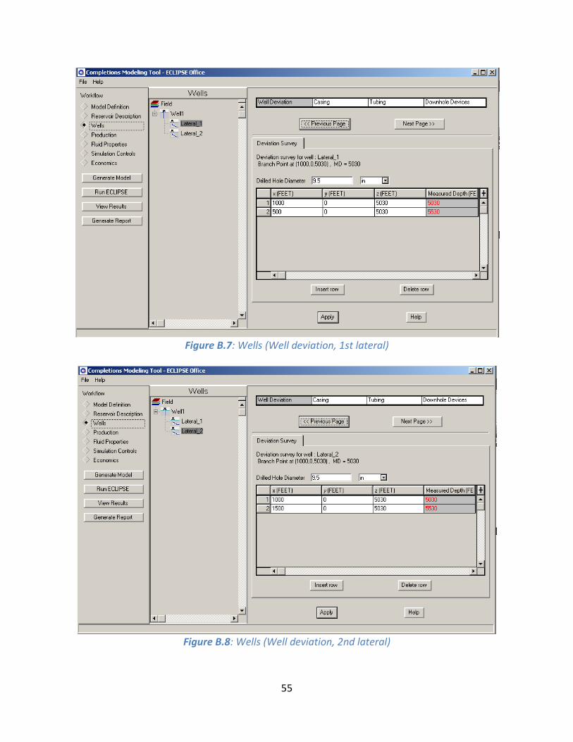
Figure B.7: Wells (Well deviation, 1st lateral)
Figure B.8: Wells (Well deviation, 2nd lateral)

56
Figure B.9: Wells (Casing)
Figure B.10: Wells (Tubing)

57
Figure B.11: Production
Figure B.12: Fluid properties (PVT correlations)

58
Figure B.13: Fluid properties (Advanced)
Figure B.14: Simulation controls (Gridding)

59
Figure B.15: Simulation controls (Tuning)
Figure B.16: Economics

60
Setting the control mode to constant gas production (same as obtained using the pseudo-
steady state gas flow rate equation), the results were obtained.
Figure B.17: Gas rate profile from ECLIPSE results

61
Figure B.18: Field pressure profile from ECLIPSE results

62
Figure B.19: Bottomhole pressure profile from ECLIPSE results
The pseudo-steady state zone was identified from the bottom hole pressure profile as evident
by a constant change in pressure (straight line decline) and is illustrated below:

63
Figure B.20: Bottomhole pressure profile showing straight line decline

64
Figure B.21: Field pressure profile showing selected point in the pseudosteady state period
Picking pressures from both bottom hole and reservoir profiles at a particular time, the gas
production rate was recalculated using the equations. Resulting values were similar with a
percentage error of about 6%.

65
Typical pressures and production rate profiles at constant bottomhole pressure(including
deliverability constant A calculation):
Table B.1: Pressure and rate profiles for base case at xe/ye =1 with A values
Xe/Ye=1
TIME FPR WBHP:WELL1WGPR:WELL1WPI:WELL1A=(pr^2-pwf^2)/q
(DAYS) (PSIA) (PSIA) (MSCF/DAY)
0 2001.814 2001.814 0 0
1 1953.406 500 52404.36 52.49987 68.04389011
2.2 1902.696 500 45891.92 50.18465 73.43892876
3.64 1846.873 500 42313.79 48.81127 74.70236991
5.368 1785.157 500 39193.65 47.54726 74.93014103
7.4416 1717.331 500 36051.41 46.20619 74.87160247
9.92992 1643.508 500 32781.48 44.72971 74.7714794
12.9159 1564.068 500 29392.93 43.10166 74.72237824
16.49908 1479.666 500 25937.96 41.32454 74.771156
20.7989 1391.236 500 22490.21 39.4139 74.94535835
25.89945 1300.907 500 19163.45 37.41547 75.26615191
31 1222.409 500 16442.26 35.64339 75.67600176
37.12066 1142.012 500 13829.04 33.79975 76.23016212
44.46545 1061.213 500 11387.5 31.92183 76.94166444
53.23272 982.0283 500 9180.849 30.06127 77.81192508
62 916.1876 500 7491.19 28.50267 78.67904624
72.52073 852.1014 500 5975.59 26.97933 79.67024811
82.76037 800.6285 500 4852.288 25.75431 80.58176986
93 757.7945 500 3981.943 24.73443 81.43071886
105.2876 716.0877 500 3191.06 23.7425 82.34932635
114.6438 688.9201 500 2705.95 23.09742 83.00631781
124 665.514 500 2307.664 22.54423 83.59487096
135.2275 641.9918 500 1924.649 21.98777 84.25094495
145.1137 624.0888 500 1645.696 21.56626 84.75855646
155 608.7 500 1413.871 21.20457 85.23809923
166.8635 593.1132 500 1186.898 20.83942 85.75569764
176.4318 582.0855 500 1031.369 20.58235 86.12198054
186 572.4742 500 898.846 20.35801 86.47386882
197.4819 562.6401 500 766.3261 20.12895 86.86109774
207.2409 555.3311 500 669.825 19.95904 87.17587348
217 548.9161 500 586.5344 19.81017 87.47800834
228.7109 542.2542 500 501.6149 19.65618 87.79569924
238.3554 537.4266 500 440.9295 19.54471 88.05804724
248 533.1773 500 388.1156 19.4467 88.31915349
259.5735 528.7869 500 334.1596 19.34557 88.62716035
269.2867 525.538 500 294.631 19.27083 88.89157933
279 522.6707 500 260.0284 19.20494 89.16209914
290.6559 519.7005 500 224.4643 19.13676 89.49578134
300.3279 517.5205 500 198.5417 19.08676 89.79180226
310 515.5909 500 175.726 19.04254 90.10628712
321.6065 513.5862 500 152.1478 18.99662 90.50912525
335 511.622 500 129.173 18.95168 91.0183383

66
Pressures and production rate profiles analyses:
xe/ye for base case scenario:
Table B.2: AH/AV values for base case at different xe/ye values
xe/ye for 4000000ft drainage area:
Xe/Ye h A AV AH AH/AV L/2Xe
1 60 2000000 74.77148 39.37909 0.526659 0.25
1 60 2000000 74.77148 24.07294 0.321954 0.5
1 60 2000000 74.77148 16.72308 0.223656 0.75
Xe/Ye h A AV AH AH/AV L/2Xe
2 60 2000000 77.11218 33.52636 0.434774 0.25
2 60 2000000 77.11218 18.57235 0.240849 0.5
2 60 2000000 77.11218 11.03715 0.143131 0.75
Xe/Ye h A AV AH AH/AV L/2Xe
5 60 2000000 91.38722 36.13112 0.395363 0.25
5 60 2000000 91.38722 18.07394 0.197773 0.5
5 60 2000000 91.38722 7.599936 0.083162 0.75

67
Table B.3: AH/AV values for 4000000ft drainage area
The table below shows how the total skin factor of a horizontal well changes with changes in
well length and drainage area aspect ratio.
Table B.4.1: Total horizontal well skin factor for A=2000000ft2
Xe/Ye h A AV AH AH/AV L/2Xe
1 60 2000000 78.83854 35.35144 0.448403 0.25
1 60 2000000 78.83854 21.38375 0.271235 0.5
1 60 2000000 78.83854 14.59482 0.185123 0.75
Xe/Ye h A AV AH AH/AV L/2Xe
2 60 2000000 80.63957 29.5891 0.36693 0.25
2 60 2000000 80.63957 16.10817 0.199755 0.5
2 60 2000000 80.63957 9.28085 0.115091 0.75
Xe/Ye h A AV AH AH/AV L/2Xe
5 60 2000000 90.43511 29.88688 0.330479 0.25
5 60 2000000 90.43511 14.59054 0.161337 0.5
5 60 2000000 90.43511 5.987876 0.066212 0.75
xe/ye 1 1 1 2 2 2 5 5 5
2xe 1414.214 1414.214 1414.214 2000 2000 2000 3162.278 3162.278 3162.278
L 353.5534 707.1068 1060.66 500 1000 1500 790.5694 1581.139 2371.708
rev 797.8846 797.8846 797.8846 797.8846 797.8846 797.8846 797.8846 797.8846 797.8846
reh 881.8544 958.496 1029.447 914.3801 1017.626 1111.32 975.7107 1125.79 1258.092
a 890.7576 991.634 1099.853 931.6248 1080.777 1244.147 1016.532 1271.952 1560.47
rw' 88.38835 176.7767 265.165 125 250 375 197.6424 395.2848 592.927
s -5.40808 -6.10123 -6.50669 -5.75465 -6.4478 -6.85327 -6.2128 -6.90595 -7.31141
LD 0.931695 1.86339 2.795085 1.317616 2.635231 3.952847 2.083333 4.166667 6.249999
L/2xe 0.25 0.5 0.75 0.25 0.5 0.75 0.25 0.5 0.75
SCA 4 3.2 2.65 3.7 2.7 2.5 3.8 2.75 2.4
S+SCA -1.40808 -2.90123 -3.85669 -2.05465 -3.7478 -4.35327 -2.4128 -4.15595 -4.91141
A=2000000ft2

68
Table B.4.2: Total horizontal well skin factor for A=4000000ft2
h, kV, kH:
Table B.5: AH/AV values for different h values at kv/kh = 1/10
xe/ye 1 1 1 2 2 2 5 5 5
2xe 2000 2000 2000 2828.427 2828.427 2828.427 4472.136 4472.136 4472.136
L 500 1000 1500 707.1068 1414.214 2121.32 1118.034 2236.068 3354.102
rev 797.8846 797.8846 797.8846 797.8846 797.8846 797.8846 797.8846 797.8846 797.8846
reh 914.3801 1017.626 1111.32 958.496 1095.815 1217.745 1040.505 1236.399 1405.245
a 931.6248 1080.777 1244.147 991.634 1215.137 1465.778 1118.087 1508.812 1957.169
rw' 125 250 375 176.7767 353.5535 530.33 279.5085 559.017 838.5255
s -5.75465 -6.4478 -6.85327 -6.10123 -6.79438 -7.19984 -6.55937 -7.25252 -7.65799
LD 1.317616 2.635231 3.952847 1.86339 3.726781 5.590169 2.946278 5.892557 8.838835
L/2xe 0.25 0.5 0.75 0.25 0.5 0.75 0.25 0.5 0.75
SCA 3.25 2.5 2.3 3.05 2.35 2.2 3.4 2.55 2.25
S+SCA -2.50465 -3.9478 -4.55327 -3.05123 -4.44438 -4.99984 -3.15937 -4.70252 -5.40799
A=4000000ft2
kv,kh h A AV AH AH/AV L 2XE L/2XE LD
1,10 60 2000000 77.11218 33.52636 0.434774 500 2000 0.25 1.317616
1,10 60 2000000 77.11218 18.57235 0.240849 1000 2000 0.5 2.635231
1,10 60 2000000 77.11218 11.03715 0.143131 1500 2000 0.75 3.952847
kv,kh h A AV AH AH/AV L 2XE L/2XE LD
1,10 100 2000000 46.2914 25.6614 0.554345 500 2000 0.25 0.790569
1,10 100 2000000 46.2914 14.49078 0.313034 1000 2000 0.5 1.581139
1,10 100 2000000 46.2914 9.024089 0.194941 1500 2000 0.75 2.371708
kv,kh h A AV AH AH/AV L 2XE L/2XE LD
1,10 120 2000000 38.58969 23.49269 0.608782 500 2000 0.25 0.658808
1,10 120 2000000 38.58969 13.43441 0.348135 1000 2000 0.5 1.317616
1,10 120 2000000 38.58969 8.511164 0.220555 1500 2000 0.75 1.976424

69
Table B.6: AH/AV values for different h values at kv/kh = 2/20
Table B.7: AH/AV values for different h values at kv/kh = 2/10
kv,kh h A AV AH AH/AV L 2XE L/2XE LD
2,20 60 2000000 38.67345 17.09656 0.442075 500 2000 0.25 1.317616
2,20 60 2000000 38.67345 9.611054 0.248518 1000 2000 0.5 2.635231
2,20 60 2000000 38.67345 5.780181 0.149461 1500 2000 0.75 3.952847
kv,kh h A AV AH AH/AV L 2XE L/2XE LD
2,20 100 2000000 23.22789 13.06058 0.56228 500 2000 0.25 0.790569
2,20 100 2000000 23.22789 7.53128 0.324234 1000 2000 0.5 1.581139
2,20 100 2000000 23.22789 4.781046 0.205832 1500 2000 0.75 2.371708
kv,kh h A AV AH AH/AV L 2XE L/2XE LD
2,20 120 2000000 19.3709 11.93893 0.616333 500 2000 0.25 0.658808
2,20 120 2000000 19.3709 6.97219 0.359931 1000 2000 0.5 1.317616
2,20 120 2000000 19.3709 4.507652 0.232702 1500 2000 0.75 1.976424
kv,kh h A AV AH AH/AV L 2XE L/2XE LD
2,10 60 2000000 77.11218 29.77397 0.386112 500 2000 0.25 1.317616
2,10 60 2000000 77.11218 16.40022 0.21268 1000 2000 0.5 2.635231
2,10 60 2000000 77.11218 9.48982 0.123065 1500 2000 0.75 3.952847
kv,kh h A AV AH AH/AV L 2XE L/2XE LD
2,10 100 2000000 46.2914 22.21986 0.48 500 2000 0.25 0.790569
2,10 100 2000000 46.2914 12.38444 0.267532 1000 2000 0.5 1.581139
2,10 100 2000000 46.2914 7.510256 0.162239 1500 2000 0.75 2.371708
kv,kh h A AV AH AH/AV L 2XE L/2XE LD
2,10 120 2000000 38.58969 20.21456 0.523833 500 2000 0.25 0.658808
2,10 120 2000000 38.58969 11.35303 0.294199 1000 2000 0.5 1.317616
2,10 120 2000000 38.58969 7.001782 0.181442 1500 2000 0.75 1.976424

70
For LD for xe/ye = 1:
Table B.8: AH/AV values for different LD values for xe/ye = 1 (kv/kh = constant)
Table B.9: AH/AV values for different LD values for xe/ye = 1 (h = constant)
kv/kh h A AV AH AH/AV L 2XE L/2XE LD
0.1 55.90116 2000000 83.75037 45.72022 0.545911 353.55 1414.214 0.25 1
0.1 111.8023 2000000 41.90689 20.11248 0.479933 707.1 1414.214 0.5 1
0.1 167.7035 2000000 27.97355 12.44478 0.444877 1060.65 1414.214 0.75 1
kv/kh h A AV AH AH/AV L 2XE L/2XE LD
0.1 27.95058 2000000 167.1624 66.50045 0.397819 353.55 1414.214 0.25 2
0.1 55.90116 2000000 83.75037 26.35369 0.31467 707.1 1414.214 0.5 2
0.1 83.85175 2000000 55.81836 14.98783 0.268511 1060.65 1414.214 0.75 2
kv/kh h A AV AH AH/AV L 2XE L/2XE LD
0.1 18.63372 2000000 251.6255 88.48958 0.351672 353.55 1414.214 0.25 3
0.1 37.26744 2000000 125.4932 33.08806 0.263664 707.1 1414.214 0.5 3
0.1 55.90116 2000000 83.75037 17.97502 0.214626 1060.65 1414.214 0.75 3
kv/kh h A AV AH AH/AV L 2XE L/2XE LD
0.115202 60 2000000 78.03051 42.89476 0.549718 353.55 1414.214 0.25 1
0.028801 60 2000000 78.03051 34.73364 0.445129 707.1 1414.214 0.5 1
0.0128 60 2000000 78.03051 30.08603 0.385567 1060.65 1414.214 0.75 1
kv/kh h A AV AH AH/AV L 2XE L/2XE LD
0.460809 60 2000000 78.03051 32.62421 0.418096 353.55 1414.214 0.25 2
0.115202 60 2000000 78.03051 24.70465 0.316602 707.1 1414.214 0.5 2
0.051201 60 2000000 78.03051 20.22076 0.259139 1060.65 1414.214 0.75 2
kv/kh h A AV AH AH/AV L 2XE L/2XE LD
1.03682 60 2000000 78.03051 29.10804 0.373034 353.55 1414.214 0.25 3
0.259205 60 2000000 78.03051 21.25794 0.272431 707.1 1414.214 0.5 3
0.115202 60 2000000 78.03051 16.84891 0.215927 1060.65 1414.214 0.75 3

71
For LD for xe/ye = 2:
Table B.10: AH/AV values for different LD values for xe/ye = 2 (kv/kh = constant)
Table B.11: AH/AV values for different LD values for xe/ye = 2 (h = constant)
kv/kh h A AV AH AH/AV L 2XE L/2XE LD
0.1 79.05694 2000000 58.50502 28.8808 0.493647 500 2000 0.25 1
0.1 158.1139 2000000 29.31548 12.09994 0.412749 1000 2000 0.5 1
0.1 237.1708 2000000 19.59463 7.156631 0.365234 1500 2000 0.75 1
kv/kh h A AV AH AH/AV L 2XE L/2XE LD
0.1 39.52847 2000000 117.1103 43.02205 0.367363 500 2000 0.25 2
0.1 79.05694 2000000 58.50502 16.12481 0.275614 1000 2000 0.5 2
0.1 118.5854 2000000 39.04414 8.541682 0.21877 1500 2000 0.75 2
kv/kh h A AV AH AH/AV L 2XE L/2XE LD
0.1 26.35231 2000000 175.2055 56.8557 0.324509 500 2000 0.25 3
0.1 52.70463 2000000 87.78705 19.94745 0.227225 1000 2000 0.5 3
0.1 79.05694 2000000 58.50502 9.826241 0.167956 1500 2000 0.75 3
kv/kh h A AV AH AH/AV L 2XE L/2XE LD
0.0576 60 2000000 77.11218 37.20946 0.482537 500 2000 0.25 1
0.0144 60 2000000 77.11218 28.69255 0.372089 1000 2000 0.5 1
0.0064 60 2000000 77.11218 23.46245 0.304264 1500 2000 0.75 1
kv/kh h A AV AH AH/AV L 2XE L/2XE LD
0.2304 60 2000000 77.11218 29.1091 0.37749 500 2000 0.25 2
0.0576 60 2000000 77.11218 20.73447 0.268887 1000 2000 0.5 2
0.0256 60 2000000 77.11218 15.56279 0.20182 1500 2000 0.75 2
kv/kh h A AV AH AH/AV L 2XE L/2XE LD
0.5184 60 2000000 77.11218 26.10432 0.338524 500 2000 0.25 3
0.1296 60 2000000 77.11218 17.69884 0.229521 1000 2000 0.5 3
0.0576 60 2000000 77.11218 12.57746 0.163106 1500 2000 0.75 3

72
NOMENCLATURE
s => equivalent negative skin factor due to either well stimulation or horizontal well,
dimensionless
sm => mechanical skin factor, dimensionless
sCA => shape-related skin factor, dimensionless
c’ => shape factor conversion constant, dimensionless
k => permeability, millidarcy
kh => horizontal permeability, millidarcy
kv => vertical permeability, millidarcy
h => reservoir height, feet
pR => average reservoir pressure, pounds per square inches
pwf => well flowing pressure, pounds per square inches
qg => gas flow rate, thousand standard cubic feet per day
T => reservoir temperature, Rankin
µ => gas viscosity at well flowing conditions, centipoise
z => gas compressibility factor evaluated at some average pressure between pR and pwf,
dimensionless
β’ => high velocity flow coefficient, per foot
g => gas gravity, dimensionless
rw => wellbore radius, feet
hp => perforated interval, feet
ka => permeability in near wellbore region, millidarcy
AC’ => 0.738 for a rectangular drainage area, dimensionless
LD => dimensionless well length
xe = > drainage radius in the x direction
ye => drainage radius in the y direction
DH => horizontal well turbulence factor

73
DV => vertical well turbulence factor
AH => deliverability constant A value for horizontal well
AV => deliverability constant A value for vertical well

74
REFERENCES
Chen, W. and Zhu, D.: “A Comprehensive Model of Multilateral Well Deliverability” SPE 64751,
2000.
Chase, R.W. and Steffy, C. R.: “Predicting Horizontal Gas Well Deliverability Using Dimensionless
IPR Curves” SPE 91101, 2004.
Wang, X. and Economides, M. J.: “Horizontal Well Deliverability with Turbulence Effects” SPE
121382, 2009.
"Natural gas." Encyclopædia Britannica. Encyclopædia Britannica Online. Encyclopædia
Britannica, 2011. Web. 26 Apr. 2011.
<http://www.britannica.com/EBchecked/topic/406163/natural-gas>.
Cho, H. and Shah, S.: “Prediction of Specific Productivity Index for Long Horizontal Wells”, SPE
67237, 2001.
Joshi, S.: “Horizontal Well Technology”, PennWell, 1991.
“ECLIPSE Reservoir Simulation” www.slb.com,
<http://www.slb.com/services/software/reseng.aspx>.
Chaudhri, A. U.: “Gas Well Testing Handbook”, Elsevier Science, 2003.
Fetkovich, M. J., and M. E. Vienot. “Shape Factors, CA, Expressed as a Skin, sCA,” J. Petroleum
Technol. (Feb. 1979) 211-16
Golan, M., and Whitson, C. H., Well Performance, International Human Resources Development
Corporation, Boston, 1986.