PREDICTING HARD DRIVE FAILURES IN COMPUTERCLUSTERS

By

ROBIN WESLEY FEATHERSTUN

A Thesis Submitted to the Graduate Faculty of

WAKE FOREST UNIVERSITY

in Partial Fulfillment of the Requirements

for the Degree of

MASTER OF SCIENCE

in the Department of Computer Science

May 2010

Winston-Salem, North Carolina

Approved By:

Dr. Errin Fulp, Ph.D., Advisor

Examining Committee:

Dr. David John, Ph.D., Chairperson

Dr. William Turkett, Ph.D.

Acknowledgements

First, I must thank my family. My parents deserve obvious thanks for making,raising, and supporting me. I also have to thank them for the often unexpected littletreats, such as sending me a spare box of Girl Scout cookies during final exams.Thank you to my brother for providing an example to look up to. Thank you tomy aunt, Mrs. Robin Bowie for the words of encouragement. Also, thank you Benand Kristin Stallbaumer for providing a place to sleep last summer during the crosscountry drive to Richland, Washington.

Thanks to all of my friends who have supported me not only through grad school,but my entire education. Most recently, thanks to Brian Williams and Greg Galantefor providing hours of bad video games, movies, and TV shows for entertainmentand random weekend trips to foreign countries. Thanks to all of the other graduatestudents for the lounge banter and weekly basketball games.

I must thank Wake Forest for accepting me not only for undergraduate, but alsofor graduate school. I have learned a lot both academically and personally since Iarrived here six years ago.

Thanks to entire faculty of the Department of Computer Science, especially mycommittee members. Specifically, thanks to Dr. William Turkett, who taught thefirst computer science class I ever took. Thank you to Dr. Jennifer Burg for advisingme on my Senior Honors Thesis during my undergraduate career. Thanks to Dr.Errin Fulp for being my advisor and for the opportunity to go to Pacific NorthwestNational Laboratory in the summer of 2009. Finally, thank you to Dr. David Johnfor filling in on my committee on very short notice.

Thank you to the Pacific Northwest National Laboratory for the contract in thesummer of 2009 and for the data used in this project.

ii

Table of Contents

Acknowledgements . . . . . . . . . . . . . . . . . . . . . . . . . . . . . . . . . . . . . . . . . . . . . . . . . . ii

List of Figures. . . . . . . . . . . . . . . . . . . . . . . . . . . . . . . . . . . . . . . . . . . . . . . . . . . . . . . v

List of Tables. . . . . . . . . . . . . . . . . . . . . . . . . . . . . . . . . . . . . . . . . . . . . . . . . . . . . . . . vi

Abstract . . . . . . . . . . . . . . . . . . . . . . . . . . . . . . . . . . . . . . . . . . . . . . . . . . . . . . . . . . . . viii

Chapter 1 Introduction . . . . . . . . . . . . . . . . . . . . . . . . . . . . . . . . . . . . . . . . . . . . 1

Chapter 2 Overview of the Syslog Event Logging System. . . . . . . . . . . 6

2.1 SMART . . . . . . . . . . . . . . . . . . . . . . . . . . . . . . . . . . 10

Chapter 3 Classification Methods . . . . . . . . . . . . . . . . . . . . . . . . . . . . . . . . . . 11

3.1 The Classification Problem . . . . . . . . . . . . . . . . . . . . . . . . 11

3.2 Pattern Recognition . . . . . . . . . . . . . . . . . . . . . . . . . . . 11

3.2.1 Design Set . . . . . . . . . . . . . . . . . . . . . . . . . . . . . 12

3.2.2 Representation . . . . . . . . . . . . . . . . . . . . . . . . . . 12

3.2.3 Adaptation . . . . . . . . . . . . . . . . . . . . . . . . . . . . 13

3.2.4 Generalization . . . . . . . . . . . . . . . . . . . . . . . . . . . 13

3.2.5 Evaluation . . . . . . . . . . . . . . . . . . . . . . . . . . . . . 13

3.3 Classification Methods . . . . . . . . . . . . . . . . . . . . . . . . . . 14

3.3.1 Unsupervised Learning . . . . . . . . . . . . . . . . . . . . . . 14

3.3.2 Supervised Learning . . . . . . . . . . . . . . . . . . . . . . . 15

3.3.3 Semi-supervised Learning . . . . . . . . . . . . . . . . . . . . 16

Chapter 4 Previous Work. . . . . . . . . . . . . . . . . . . . . . . . . . . . . . . . . . . . . . . . . . 18

4.1 Predictions Using SMART . . . . . . . . . . . . . . . . . . . . . . . . 18

4.2 Predictions for IBM BlueGene . . . . . . . . . . . . . . . . . . . . . . 20

4.3 A Naive Bayesian Approach . . . . . . . . . . . . . . . . . . . . . . . 23

4.4 Failure Trends . . . . . . . . . . . . . . . . . . . . . . . . . . . . . . . 25

4.5 Statistical Approach to Failure Prediction . . . . . . . . . . . . . . . 26

4.6 System Board Failures . . . . . . . . . . . . . . . . . . . . . . . . . . 28

4.7 Summary . . . . . . . . . . . . . . . . . . . . . . . . . . . . . . . . . 29

iii

iv

Chapter 5 New Spectrum-Kernel Based Methods for Failure Predic-

tions . . . . . . . . . . . . . . . . . . . . . . . . . . . . . . . . . . . . . . . . . . . . . . . . . . . . . . . . . . . . . . . . 30

5.1 Sequences . . . . . . . . . . . . . . . . . . . . . . . . . . . . . . . . . 30

5.1.1 Sliding Window . . . . . . . . . . . . . . . . . . . . . . . . . . 31

5.1.2 Spectrum Kernel . . . . . . . . . . . . . . . . . . . . . . . . . 32

5.2 Tag Based Features . . . . . . . . . . . . . . . . . . . . . . . . . . . . 34

5.2.1 Tags With Timing Information . . . . . . . . . . . . . . . . . 37

5.3 Message Based Approaches . . . . . . . . . . . . . . . . . . . . . . . . 38

5.3.1 Using Keystrings as Features . . . . . . . . . . . . . . . . . . . 41

5.3.2 Keystrings With Timing Information . . . . . . . . . . . . . . 43

5.4 Combining Tag-based and Keystring-basedApproaches . . . . . . . . . . . . . . . . . . . . . . . . . . . . . . . . 43

Chapter 6 Support Vector Machines . . . . . . . . . . . . . . . . . . . . . . . . . . . . . . . 45

6.1 The Data . . . . . . . . . . . . . . . . . . . . . . . . . . . . . . . . . 45

6.2 Optimal Hyperplane . . . . . . . . . . . . . . . . . . . . . . . . . . . 45

6.3 SVM Kernels . . . . . . . . . . . . . . . . . . . . . . . . . . . . . . . 48

6.3.1 Linear Kernel . . . . . . . . . . . . . . . . . . . . . . . . . . . 49

6.3.2 Polynomial Kernel . . . . . . . . . . . . . . . . . . . . . . . . 50

6.3.3 Radial Basis Function . . . . . . . . . . . . . . . . . . . . . . 50

6.4 Theoretical Complexity . . . . . . . . . . . . . . . . . . . . . . . . . . 51

Chapter 7 Experimental Results . . . . . . . . . . . . . . . . . . . . . . . . . . . . . . . . . . . 52

7.1 Introduction . . . . . . . . . . . . . . . . . . . . . . . . . . . . . . . . 52

7.2 Tag Numbers . . . . . . . . . . . . . . . . . . . . . . . . . . . . . . . 54

7.2.1 Preprocessing . . . . . . . . . . . . . . . . . . . . . . . . . . . 54

7.3 Keystring Approaches . . . . . . . . . . . . . . . . . . . . . . . . . . 65

7.3.1 Preprocessing . . . . . . . . . . . . . . . . . . . . . . . . . . . 65

7.3.2 Results Using Keystring Sequences Without Time Information 66

7.3.3 Keystring Sequences Using Time . . . . . . . . . . . . . . . . 68

7.4 Combination of Keystrings and Tag Sequences . . . . . . . . . . . . . 69

Chapter 8 Conclusions and Future Work . . . . . . . . . . . . . . . . . . . . . . . . . . . 72

8.1 Comparison of Methods . . . . . . . . . . . . . . . . . . . . . . . . . 74

8.1.1 Balance Between True Positives and Failures Predicted . . . . 75

8.1.2 Space Requirements . . . . . . . . . . . . . . . . . . . . . . . 75

8.1.3 The Best Method . . . . . . . . . . . . . . . . . . . . . . . . . 79

8.2 Future Work . . . . . . . . . . . . . . . . . . . . . . . . . . . . . . . . 80

References . . . . . . . . . . . . . . . . . . . . . . . . . . . . . . . . . . . . . . . . . . . . . . . . . . . . . . . . . . 83

List of Figures

2.1 An example distribution of tag values across multiple hosts . . . . . . 8

2.2 An example distribution of tag values over time for a single host . . . 9

5.1 An example computation of sequence numbers . . . . . . . . . . . . . 33

6.1 An illustration of the optimal 2-D hyperplane . . . . . . . . . . . . . 46

6.2 An example where the data must be mapped to higher dimensions . . 47

7.1 A graph of the effect of increasing lead time (in messages) for tag-basedfeatures . . . . . . . . . . . . . . . . . . . . . . . . . . . . . . . . . . 60

7.2 A graph of the effect of increasing window size (in messages) . . . . . 62

v

List of Tables

2.1 Example entries from a syslog file . . . . . . . . . . . . . . . . . . . 6

2.2 Examples of possible syslog configurations . . . . . . . . . . . . . . . 9

5.1 A list of letters . . . . . . . . . . . . . . . . . . . . . . . . . . . . . . 32

5.2 Letter sequences using a sliding window of length 3 . . . . . . . . . . 32

5.3 Numerical assignments for letters . . . . . . . . . . . . . . . . . . . . 33

5.4 Sequence numbers where k = 3 . . . . . . . . . . . . . . . . . . . . . 34

5.5 The raw tag numbers . . . . . . . . . . . . . . . . . . . . . . . . . . . 34

5.6 The resulting feature vectors . . . . . . . . . . . . . . . . . . . . . . . 35

5.7 An example of tag-based sequence numbers . . . . . . . . . . . . . . . 37

5.8 Time Difference and Tag numbers . . . . . . . . . . . . . . . . . . . . 38

5.9 The feature vectors the result from timing information . . . . . . . . 38

5.10 The original messages . . . . . . . . . . . . . . . . . . . . . . . . . . . 39

5.11 Translation from a word to its unique number . . . . . . . . . . . . . 40

5.12 The translated messages . . . . . . . . . . . . . . . . . . . . . . . . . 40

5.13 The original messages . . . . . . . . . . . . . . . . . . . . . . . . . . . 42

5.14 A list of example keystrings . . . . . . . . . . . . . . . . . . . . . . . 42

5.15 The converted messages from Table 5.13 using the keystrings in Table5.14 . . . . . . . . . . . . . . . . . . . . . . . . . . . . . . . . . . . . 42

5.16 The resulting keystring list from Table 5.15 . . . . . . . . . . . . . . . 42

7.1 The original messages . . . . . . . . . . . . . . . . . . . . . . . . . . . 55

7.2 The reduced messages . . . . . . . . . . . . . . . . . . . . . . . . . . 55

7.3 The Effect of C Value on Linear Kernel Performance. . . . . . . . . . 58

7.4 The Effect of the D Value on Polynomial Kernel Performance. . . . . 58

7.5 The Effect of the Gamma Value on Radial Basis Function Performance 59

7.6 A comparison of sequence lengths . . . . . . . . . . . . . . . . . . . . 63

7.7 Comparing performance between features using only tags and featuresincluding time information using sequences of length 5 . . . . . . . . 64

7.8 Comparing performance between features using only tags and featuresincluding time information using sequences of length 7 . . . . . . . . 65

7.9 A comparison of keystring dictionaries . . . . . . . . . . . . . . . . . 67

7.10 Performance as sequence length increases . . . . . . . . . . . . . . . . 67

vi

vii

7.11 A comparison of the 24 keystring dictionary with and without theaddition of time information . . . . . . . . . . . . . . . . . . . . . . . 68

7.12 A comparison of tag-based and keystring-based methods . . . . . . . 69

7.13 A comparison of tag based, keystring based, and combination methods 70

Abstract

Mitigating the impact of computer failure is possible if accurate failure predictionsare provided. Resources, and services can be scheduled around predicted failure andlimit the impact. Such strategies are especially important for multi-computer systems,such as compute clusters, that experience a higher rate of failure due to the largenumber of components. However providing accurate predictions with sufficient leadtime remains a challenging problem.

This research uses a new spectrum-kernel Support Vector Machine (SVM) ap-proach to predict failure events based on system log files. These files contain mes-sages that represent a change of system state. While a single message in the filemay not be sufficient for predicting failure, a sequence or pattern of messages maybe. This approach uses a sliding window (sub-sequence) of messages to predict thelikelihood of failure. Then, a frequency representation of the message sub-sequencesobserved are used as input to the SVM. The SVM associates the messages to a classof failed or non-failed system. Experimental results using actual system log files froma Linux-based compute cluster indicate the proposed spectrum-kernel SVM approachcan predict hard disk failure with an accuracy of 80% about one day in advance.

viii

Chapter 1: Introduction

Since computers were created, their users have been struggling with both hardware

and software failures. Many of these failures are rather mundane, such as a web

browser closing any time a given web page is loaded. While the browser crash is

annoying for the user, rarely does a simple software error of this sort do any lasting

damage. If the incident does have a lasting effect, the user can always reinstall the

browser or, as an absolute worst case, the operating system.

While software errors can be rather harmless, a hardware error can be much more

catastrophic. Even such a seemingly small malfunction as a faulty fan can have

devastating effects on the rest of the system. A broken fan cripples the computer’s

cooling ability, resulting in high operating temperatures, which can cause damage to

even other hardware components. Some hardware failures, such as disk failures, can

have a massive effect on users. On a PC, a failed hard drive results in the loss of all

personal data, such as pictures, movies, songs, and text documents.

The loss of data that a PC user suffers when his or her disk crashes is paralleled in

a work environment, where very sensitive data might be lost. For example, banks keep

track of financial records. If a single hard disk fails, some portion of those financial

records will be lost, which clearly has a significant effect on whoever just had their

bank account disappear. In an effort to counteract such a situation, most PC users

and corporations back up the contents of their hard drives. A PC user most likely

uses an external hard drive to back up all of their important files. Large corporations

1

2

often use RAID technology, in which a copy of all data on one disk is kept on one or

more disks in a disk array [28].

In the bank example, since multiple copies of all records are kept on different

disks, the data can be recovered. An administrator will replace the failed hard disk

and the records will be restored to that disk from the backup. RAID technology

ensures that there is a high probability that a backup is available, but the restoration

still takes time, which means that recovering from the original disk failure is still

costly. However, consider the case of a compute cluster. These clusters consist of

multiple computers or servers, called nodes, and are used to perform massive amounts

of calculations on large data sets [2]. Scheduling processes not only balance the

computational load among different processors on a given node, but also schedule a

job to cross multiple nodes. In many cases, these processes have to write data to the

hard disk of at least one of the nodes. If the disk drive to which the job is writing

data fails, then the results of computations that have already occurred since the last

backup will be lost [28]. Therefore, the job will have to be restarted to first repeat the

calculations and then finish the job. Not only has the time that the job used already

been wasted, but other jobs may have to be preempted when the node is taken offline

for a disk replacement. As a result, all of the time used for those jobs since the most

recent backup has also been wasted [28].

Minimizing the amount of downtime that either a node or disk spends is important

when one considers the growth rate of clusters. Currently, it is simply easier to buy

more computers and add them to a cluster than it is to increase the processing speed

and power of processors. Similarly, purchasing more hard drives in an effort to increase

3

storage space is easier than the design and construction of higher-capacity hard disks.

As such, clusters are quickly growing in size in terms of both computing power and

storage space. It is predicted that by 2018, large systems could have over 800,000

disks. Out of these 800,000 disks, it is possible that 300 of them may be in a failure

state at any given time [27]. Since multicore processors are becoming more prevalent,

even one disk being unavailable means that multiple processors may be unable to

perform their work. So, if 300 disks are down, a significant number of jobs might be

adversely affected. While 300 disks is not a large percentage of the 800,000 disks,

it still means that a few hundred, or maybe even a thousand, jobs will have to be

restarted. As a result, many different people and projects will be affected. Assuming

one could predict these failure events, the distribution of work on the cluster could

be altered to avoid those 300 disks before they failed or pause the jobs while the

necessary data is backed up and moved to a new disk. Essentially, the disk could

enter a maintenance phase before failing, and thus minimize the number of jobs that

need to be restarted.

This thesis investigates and develops a prediction technique for identifying future

disk failures. There are five steps that are common to most hardware-prediction

methods. First, some kind of historical data must be collected. Next, the data must

be examined to determine important features. These features are what the prediction

method will use to classify the data. An example of a feature is the number of times

a particular string appears in a list of strings. Third, the prediction method must

look at some subset of the data and build a model of the data. The model created by

the training step is applied to a test set and makes predictions on examples. Finally,

4

once the prediction is complete, one must measure the success of that prediction to

see whether or not the model created was effective.

There are four main goals that the approach in this thesis must satisfy. First,

the method must provide effective predictions. Second, the approach must use as few

sources of information as possible. The more specific the data set becomes, the less

general the method becomes. For example, if part of the data were gathered from a

utility only available on OS X 1, then the proposed method would be useable only on

OS X. The third goal is related to the second, in that classifying the data should be

both simple and fast. For example, if one could use a classifier to predict disk failures

one day in advance, but the classifier took two days to run, then that method would

be ineffective. Using fewer types of information should increase the ease and speed of

the classification step. Finally, the approach should also be able to predict the disk

failure with significant lead time, such as days instead of minutes.

Three metrics are commonly used to measure the successfulness of a prediction

[22]. First is accuracy, which is the total number of correct predictions divided by the

total number of inputs. Accuracy gives a measure of how many of the predictions,

both positive and negative, were correct. The second metric is precision. Precision

is the number of true positive predictions over all positive predictions. Precision

therefore measures how many of the predicted positives actually were positive. A

high precision score results in fewer false positives, such as a disk being predicted to

fail which does not fail. Finally, recall is the number of true positive predictions over

the total number of positive inputs. Recall measures how many of the actual positives

1OS X is a trademark of Apple, Inc

5

inputs, in this case disk failures, were classified correctly.

The proposed prediction process uses the syslog event logging service as data to

predict failure events. The syslog facility is common to all Linux distributions as

well as Unix variants. Also, syslog is the only source of information used, so any

system using Linux or Unix should be able to employ this method. From this data, a

Support Vector Machine [8] creates a model of the data which isolates patterns of log

information that indicate disk failures. Using this approach, a system administrator

would thus have an opportunity to reschedule jobs and back up disks before the disk

fails. The main focus of this approach is to predict disk failures at least one day

before the failure. This lead time will give administrators enough time to make any

necessary changes to the scheduling process or ensure that they can obtain another

hard drive of the correct model [13]. This thesis also explores whether or not one

can gain increased prediction accuracy by reducing the amount of lead time before a

failure [13].

The rest of this document is organized as follows. Chapter 2 contains an overview

of the syslog event log system. A discussion of classification methods is contained

in Chapter 3. Chapter 4 holds a literature review. Chapter 5 introduces the clas-

sification approach developed in this thesis. Chapter 6 details the SVM approach

to classification, while chapter 7 describes experimental results. Finally, chapter 8

presents conclusions drawn from the experimental results and discusses opportunities

for future work.

Chapter 2: Overview of the Syslog Event

Logging System

Syslog is a standard Unix logging facility, which means that every computer run-

ning Linux has syslog by default [21]. The ubiquity of syslogmeans that performing

an analysis on syslog data allows for the creation of a failure prediction approach

which can be used by anyone using a Linux or Unix system. Syslog records any

change of system state, such as a login or a program failure. Ideally, such a general

method will allow for the same procedure to be used on many different clusters with

the same accuracy.

Host Facility Level Tag Time Message

node226 daemon info 30 1205054912 ntpd 2555 synchronized to 198.129.149.215, stratum 3

node226 local4 info 166 1205124722 xinetd 2221 START: auth pid=23899 from=130.20.248.51

node165 local3 notice 157 1205308925 OSLevel Linux m165 2.6.9-42.3sp.JD4smp

node165 syslog info 46 1205308925 syslogd restart.

Table 2.1: Example entries from a syslog file

As seen in Table 2.1, the standard syslog message contains six fields [21]. The

first field identifies the host posting the message. In a Linux cluster, many machines

perform operations and are governed by a smaller number of control nodes. Events

occur on each node and are logged on that node. Events logged on a particular node

are also forwarded to a central syslog server on a central node. Since many different

nodes are reporting syslog events to a central node, the central node must be able

to indicate which node posted a message. As such, the host that posted the message

is recorded to indicate that the given event occurred on that system.

6

7

The next three fields are intimately related. First, there is the facility field. The

facility assigns a broad classification to the sender of the message. For example, two

of the available facilities are user-level and local. Messages which originate from a

program such as xine might be created citing either the user or local facilities [21].

The level field is next. The level field gives a general idea of the type of message,

such as a notice or an alert. The level field is an indication of the importance of

the message. For example, a message with a level of alert is more important than

a message whose level is info. Finally, there is the tag field. The tag is a numerical

representation of the importance of the message. The level field is a coarse-grained

indication of the importance of the message, but the tag message allows for a fine-

grained indication. The tag number is an integer, where a lower number indicates a

higher importance. For example, a message with a tag number of 1 is more urgent

than a tag number of 20. Since two messages with the same level can have different

tag numbers, the messages can still be ranked in order of importance. Figures 2.1 and

2.2 show an example distribution of the number of occurrences of each tag number

as a percentage of all tag numbers and the distribution of tag numbers over time,

respectively. Figure 2.1 indicates that the majority of messages contain a high tag

number, meaning that most of the logged messages are of low criticality. Examples

of low criticality messages include notifications that a program has started or a disk

has been unmounted. Each circle in Figure 2.2 represents a single syslog message.

The circle’s position on the y-axis indicates the tag number of a particular message.

Figure 2.1 suggests that the majority of the tag numbers in a file should have high

tag numbers. The majority of the tag numbers in Figure 2.2 are centered near a tag

8

0 50 100 150 2000

0.1

0.2

0.3

0.4

0.5

0.6

tag value

perc

ent o

f all

mes

sage

sDistribution of Tag Values

Figure 2.1: An example distribution of tag values across multiple hosts

value of 148. Messages containing a tag value of 148 are so plentiful that Figure 2.2

appears to have a solid line where y = 148.

The next field in Table 2.1 is the time field, which records the time at which the

message was posted. It is common in Linux to use Linux epoch time; however there,

are other formats available. The timestamp of a particular message is determined by

the node which posts the message.

The final field is the message field. The message field consists of a plain text string

of varying length. The message is an explicit description of the associated event. The

other fields only indicate how important the event was and when it took place. The

message field tells an observer that the event was, for example, a login attempt or a

disk failure.

9

1.1778 1.1779 1.178 1.1781 1.1782 1.1783 1.1784 1.1785

x 109

0

50

100

150

200

time (seconds)

tag

num

ber

h198.129.146.158

Figure 2.2: An example distribution of tag values over time for a single host

There are many different ways to set up and customize syslog. These customiza-

tions include cosmetic differences, such as the format of the timestamp, or more

significant difference, such as the omission of entire fields. A few examples of differ-

ent configurations can be seen in Table 2.2. The first two configurations are the same,

except that the first records the timestamp in epoch time while the second timestamp

explicitly states the date. The configuration in the third row has left out the level

field.

Host Facility Level tag Time Message

node52 local4 info 166 1172744793 xinetd 905 START shell pid=16548 from=198.129.149.312

node52 kern alert 5 13-May-2009 01:50:36PM kernel raid5: Disk failure of sde1, disabling device.

node52 kern 6 1172746564 kernel md: updating m9 RAID superblock on device

Table 2.2: Examples of possible syslog configurations

10

2.1 SMART

SMART 1 messages record and report information that relates solely to hard disks,

such as their current health and performance. Since the focus of this research is

the prediction of hard drive failures, SMART data is of particular interest. The

acronym SMART stands for Self-Monitoring Analysis and Reporting Technology and

is deployed with most modern ATA and SCSI drives [1]. Since SMART disks monitor

health and performance information, they are able to report and possibly predict

hard drive problems. Some of the attributes monitored by SMART are the current

temperature, the number of scan errors, and the number of hours for which a disk has

been online. SMART checks the disk’s status every 30 minutes and passes along any

information regarding the possibility of an upcoming failure to syslog. Pinheiro et

al. have shown that solely using SMART data as a source for disk failure prediction is

ineffective [24]. Therefore, the research detailed in this thesis will use all syslog data,

including, but not limited to, SMART data, in the interest of improving prediction

performance over models which use only SMART data.

1SMART is a joint specification created by Compaq Computer Corporation; Hitachi, Ltd; IBMStorage Products Company; Maxtor Corporation; Quantum Corporation; Seagate Technology;Toshiba Corporation and Western Digital Corporation

Chapter 3: Classification Methods

3.1 The Classification Problem

In a general sense, the classification problem is an attempt to use examples that fit

into a certain category to determine whether or not an unknown example fits into

said category. In the case of this thesis, whether or not a disk fails is known. The

classification problem looks at training examples of disks that failed and disks that did

not fail. Using these examples, one can ideally take an unlabeled example and, using

the knowledge gained from the labeled examples, attempt to classify the unlabeled

example as either a failure or non-failure event.

In 1936, R.A. Fisher [12] became the first to suggest an algorithm for the classifi-

cation problem. Fisher compared two ways of classifying populations. The first was a

Bayesian classifier [25] which required quadratic time. Fischer then showed a method

for reducing the classification to a linear function [12].

3.2 Pattern Recognition

One of the methods used for solving the classification problem, which this research

employs, is pattern recognition. The goal of pattern recognition is to take a set of

data and discover trends which can assist in the correct classification of that data.

For example, if the classification problem in question is trying to separate data points

into Class A and Class B, then the pattern recognition approach will attempt to find

11

12

one or more patterns of data that characterize points which fall into Class A. The

approach can then either discover patterns that perform the same function for Class

B, or it can simply state that any data which does not fall in Class A falls into Class B.

According to Duin and Pekalska [11], most, if not all, pattern recognition algorithms

follow a basis five step structure. The steps are as follows.

3.2.1 Design Set

The design set is used both to determine patterns in the data and to test how well

the discovered patterns work. Preparation of the design set includes tasks such as

removing improperly labeled inputs. For example, if a given classification problem

uses labeled photographs of oranges and apples as input, any photographs of apples

labeled as oranges must have their label changed to apple. As mentioned earlier, the

design set will be split into two subsets: the training set and the test set. Both of

these sets need to be be representative of the overall data set. For example, in the

case of this thesis, both sets need to contain data from nodes which have seen a disk

failure and nodes on which no disk has failed.

3.2.2 Representation

When first obtained, the data will not always already be in a format that is under-

standable by the pattern recognition software. During the representation stage, the

data is transformed from its original form to a form that the software can use: for

example, a list of features which are paired with a count of how many times that fea-

tures was seen. In the representation stage, one transforms the data from its original

representation into a list of features with associated counts.

13

3.2.3 Adaptation

The adaptation stage involves the alteration of the problem statement or learning

method in an attempt to enhance final recognition. Whether or not this stage is

performed depends on the problem. It is possible that the original statement of the

problem and the original method are effective or simple enough that no restatement

is needed. If, however, change is needed, the change could be as simple as omitting or

adding some data or transforming the data into a higher dimensional representation.

3.2.4 Generalization

The generalization step is where the actual pattern recognition occurs. In this stage,

a classification method would take a training set and learn from it. In the process, the

training algorithm builds a model of the data, which includes which feature vectors are

useful in making a prediction. Hopefully, this model will produce a generalized version

of what a certain class looks like, so the classification method can later correctly

recognize to which class an unlabeled example belongs.

3.2.5 Evaluation

Finally, the model produced in the generalization stage is applied to the test set. At

the basic level, the evaluation stage keeps track of how many test examples the model

classified correctly.

14

3.3 Classification Methods

While all classification methods have the same overall steps, the method in which

they perform these steps can vary greatly. All of the classification methods must

in some way attempt to build an effective model for a given problem. Ghahramani

mentions four types of learning methods: unsupervised learning, supervised learning,

reinforcement learning and game theory [14]. Reinforcement learning is the study of

how a machine interacts with its environment, receiving either a reward or punishment

for its actions. However, reinforcement learning is more closely related to decision

theory than classification. Game theory is a generalized version of reinforcement

theory in which multiple machines vie for the same reward. This thesis focuses solely

on one machine trying to correctly classify disk failures. As such, neither of these

two approaches is useful. However, supervised learning and unsupervised learning

are both closely related to the classification problem.

3.3.1 Unsupervised Learning

In unsupervised learning approaches, the classifier receives a series of unlabeled inputs

x1, x2, x3, ..., xn. For simplicity, assume that the classifier is trying to place inputs into

one of two classes, A or B. Since a given input xi is unlabeled, the classifier has no

indication to which class that specific input belongs. Ghahramani explains that, “[i]n

a sense, unsupervised learning can be thought of as finding patterns in the data above

and beyond what would be considered pure unstructured noise.” [14]

One method of unsupervised learning is clustering. Peter Dayan explains cluster-

ing using an example of using photoreceptor data to discern whether a given image

15

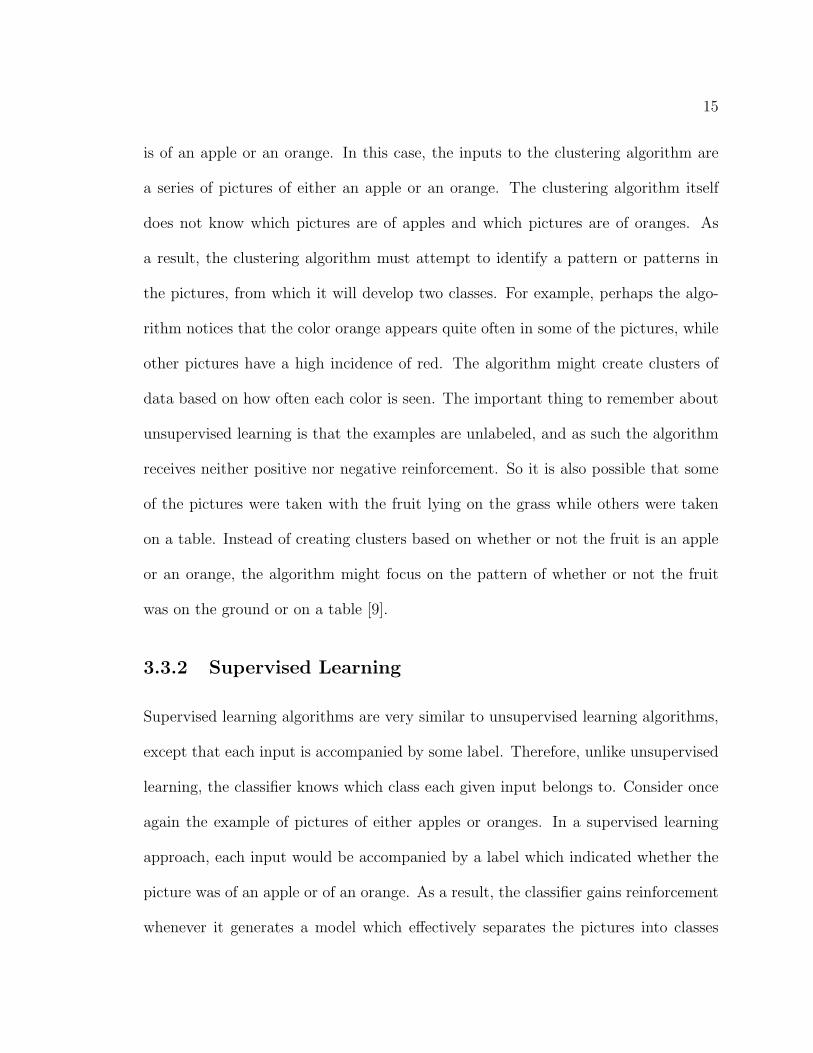
is of an apple or an orange. In this case, the inputs to the clustering algorithm are

a series of pictures of either an apple or an orange. The clustering algorithm itself

does not know which pictures are of apples and which pictures are of oranges. As

a result, the clustering algorithm must attempt to identify a pattern or patterns in

the pictures, from which it will develop two classes. For example, perhaps the algo-

rithm notices that the color orange appears quite often in some of the pictures, while

other pictures have a high incidence of red. The algorithm might create clusters of

data based on how often each color is seen. The important thing to remember about

unsupervised learning is that the examples are unlabeled, and as such the algorithm

receives neither positive nor negative reinforcement. So it is also possible that some

of the pictures were taken with the fruit lying on the grass while others were taken

on a table. Instead of creating clusters based on whether or not the fruit is an apple

or an orange, the algorithm might focus on the pattern of whether or not the fruit

was on the ground or on a table [9].

3.3.2 Supervised Learning

Supervised learning algorithms are very similar to unsupervised learning algorithms,

except that each input is accompanied by some label. Therefore, unlike unsupervised

learning, the classifier knows which class each given input belongs to. Consider once

again the example of pictures of either apples or oranges. In a supervised learning

approach, each input would be accompanied by a label which indicated whether the

picture was of an apple or of an orange. As a result, the classifier gains reinforcement

whenever it generates a model which effectively separates the pictures into classes

16

based on whether the subject is of an apple or an orange. The classifier will not focus

on placement of the fruit on the ground instead of the table, like an unsupervised

classifier might [7].

An example of supervised learning is the nearest neighbor algorithm. The nearest

neighbor approach examines each unlabeled data point and computes the shortest

distance from the unlabeled point to any labeled point. The unlabeled point is then

considered to be in the class of the labeled point. Returning to the apple and oranges

example, the nearest neighbor algorithm takes as input a collection of pictures which

are labeled either as being of apples or of oranges. This process results in a collection of

data points, some labeled as oranges and some as apples. Each unlabeled photograph

is then analyzed and the distance between that photograph and every other data

point is computed. Finally, the unlabeled photo is assigned the label of the nearest

data point. For instance, if the nearest data point was a picture of an apple, then the

unlabeled point will be labeled as an apple [34].

3.3.3 Semi-supervised Learning

Semi-supervised learning is an alternative to supervised and unsupervised learning

which meets both approaches in the middle. Like in supervised learning, the input

set is accompanied by labels. However, not all inputs are required to have a label.

Under this approach, the inputs which have labels are generally separated from the

unlabeled inputs. A model is then built using one of two methods.

In a self-learning approach, a model is built using the labeled examples. The

algorithm then labels a random subset of the unlabeled examples using this model

17

and assumes that the labels are applied to the correct class. Then, a new model is

built using both the originally labeled examples and the labels assigned by the old

model. This process repeats until all of the unlabeled inputs have labels.

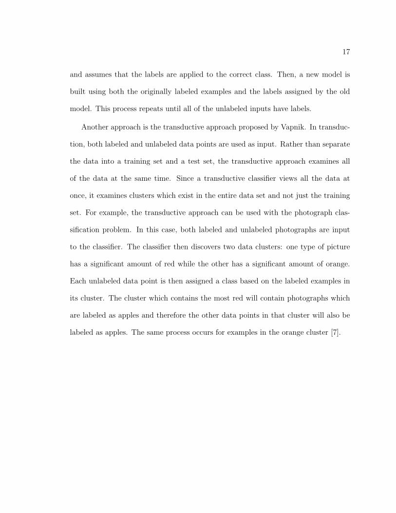
Another approach is the transductive approach proposed by Vapnik. In transduc-

tion, both labeled and unlabeled data points are used as input. Rather than separate

the data into a training set and a test set, the transductive approach examines all

of the data at the same time. Since a transductive classifier views all the data at

once, it examines clusters which exist in the entire data set and not just the training

set. For example, the transductive approach can be used with the photograph clas-

sification problem. In this case, both labeled and unlabeled photographs are input

to the classifier. The classifier then discovers two data clusters: one type of picture

has a significant amount of red while the other has a significant amount of orange.

Each unlabeled data point is then assigned a class based on the labeled examples in

its cluster. The cluster which contains the most red will contain photographs which

are labeled as apples and therefore the other data points in that cluster will also be

labeled as apples. The same process occurs for examples in the orange cluster [7].

Chapter 4: Previous Work

Failure prediction has gained increased attention from the research community.

The types of predictions range from disk failures [13] to system board failures [33].

These approaches typically examine some form of event logs to predict future fail-

ures. The approaches isolate some window of messages and identify some form of

information that can be used to identify future failures. Many different classifica-

tion approaches have been used, including SVMs [13], Bayesian classifiers [15], and

rule-based classifiers [20].

4.1 Predictions Using SMART

Greg Hamerly and Charles Elkan tackle the failure prediction problem using two types

of Bayesian networks on a collection of SMART data [15]. Their first approach uses

an unsupervised Bayesian classifier. The second approach explores a semi-supervised

naive Bayes classifier. The unsupervised classifier builds a model using examples both

of disks operating normally and disks which failed. In this case, it is assumed that the

number of abnormalities is not large enough to significantly alter the model of normal

data. The supervised method removes all abnormal data points to ensure that the

anomalies do not significantly alter the model.

Hamerly and Elkan’s approach views a disk failure as an anomaly detection prob-

lem. Every disk drive which does not fail is used to build a profile of the majority

18

19

class. Unlike the approach developed by this thesis, which builds a model of both

the positive and negative classes, this approach only builds a model for the positive

class. Any example which does not fit this model is then considered to be part of the

anomaly class.

As input, the group used a series of snapshots of SMART data values for each

drive. Since SMART data fields record data cumulatively, for each snapshot, the group

recorded the difference between the current values and the values from the previous

snapshot. As a result, each snapshot contains only the changes that occurred between

snapshots.

The group performed the experiments under two assumptions: first, that one

cannot predict a disk failure any more than 48 hours before the failure; and second,

that the most desired characteristic of the model was a minimized false positive rate.

By minimizing the false positive rate, the group was trying to ensure that disks which

were predicted to fail actually did fail in an effort to minimize the cost associated with

replacing working disks.

Each experiment used 10-fold cross validation. In 10-fold cross validation, the

data is split up into 10 equal parts. Each part contains an equal number of data

points of each class. The classifier then builds a model using nine of the partitions

and tests on the remaining partition. Each of the partitions is used as the test set

once [34].The models are trained only on the disks that do not fail and which were

not predicted by SMART to fail. When tested on a data set which includes both

failure and non-failure events, the naive Bayesian approach results in 52% precision.

The advantage of this approach is that it builds a model using only data from

20

disks which do not fail. As a result, it should be able to build a model of normal

operation and classify any points which do not fit the model as being likely to fail.

Successfully performing this task would mean that a cluster which has experienced

no failures could still predict future failures.

The paper has a few disadvantages. First, the paper assumes that one cannot

predict disk failures more than 48 hours in advanced. This thesis does not make

this assumption, which means it is possible that this approach might actually predict

failures more than 2 days in advance. Another downside is that the model built in

the paper only has a 52% true positive rate.

4.2 Predictions for IBM BlueGene

Liang et al. of IBM explored solutions to this problem by using data from IBMs

BlueGene [20]. This group used data from a specialized logging facility deployed

on BlueGene. The data was gathered over the course of 142 days. The goal of the

study was to compare the prediction performance when using a rule-based classifier,

an SVM, a traditional nearest neighbor technique and a custom nearest-neighbor

technique.

The BlueGene system uses its own customized logging facility, named RAS. Each

RAS event has five fields: the severity of the event, such as warning, info, and failure;

the time the event occurred; which job posted the event; the location of the event;

and a description of the event. Logs were collected over the course of four months

[20].

The prediction approach broke up each log into equal length time windows. As

21

such, when a certain window was reached, the classifier tried to predict whether or not

there would be a failure during that time window. To make this prediction, it used

observations from some number of previously viewed windows, called the observation

windows. After a prediction had been made for the current window, the current

prediction window became an observation window. During each window, six groups

of features are tracked. First was the number of each type of event that occurred

in the current time window. Second was the number of each type of event that

occurred during the observation period. The third group analyzed the distribution

of events over the course of the observation period. The fourth group kept track

of the total time since the previous failure interval. The final group indicated the

number of times each phrase occurred, where phrase is defined as any message whose

identifying characteristics such as node number or IP address were stripped out.

Finally, the features that were seen in observation windows preceding a failure window

were separated from those features which were seen in observation windows which did

not precede a failure window.

The group then analyzed the data using three methods: a rule based classifier

named RIPPER, SVMs, and a bi-modal nearest neighbor algorithm. For RIPPER,

the team input 17 weeks of training data, from which RIPPER created a rule set.

A rule set is created by partitioning the training set into two sets: the growing set

and the pruning set. Rules are added by examining examples in the growing set. For

each positive example, such as a disk failure, a new rule is added. Rules are added

until no negative examples, such as disks which did not fail, are covered by the rule

set. Each rule is then tested on the pruning set. Any conditions for a rule that may

22

be removed and still cover only positive examples from the pruning set are discarded

[26]. This rule set was then run on different examples to test its classification ability.

The group ran a support vector machine using a radial-basis function and five-fold

cross validation. Their nearest neighbor algorithm uses three sets of data: anchor,

training, and test. The anchor data is a list of failure events. The bi-modal nearest

neighbor algorithm uses the anchor and training data to create a classifier that is

based on two thresholds instead of just one like a usual nearest neighbor algorithm

[34].

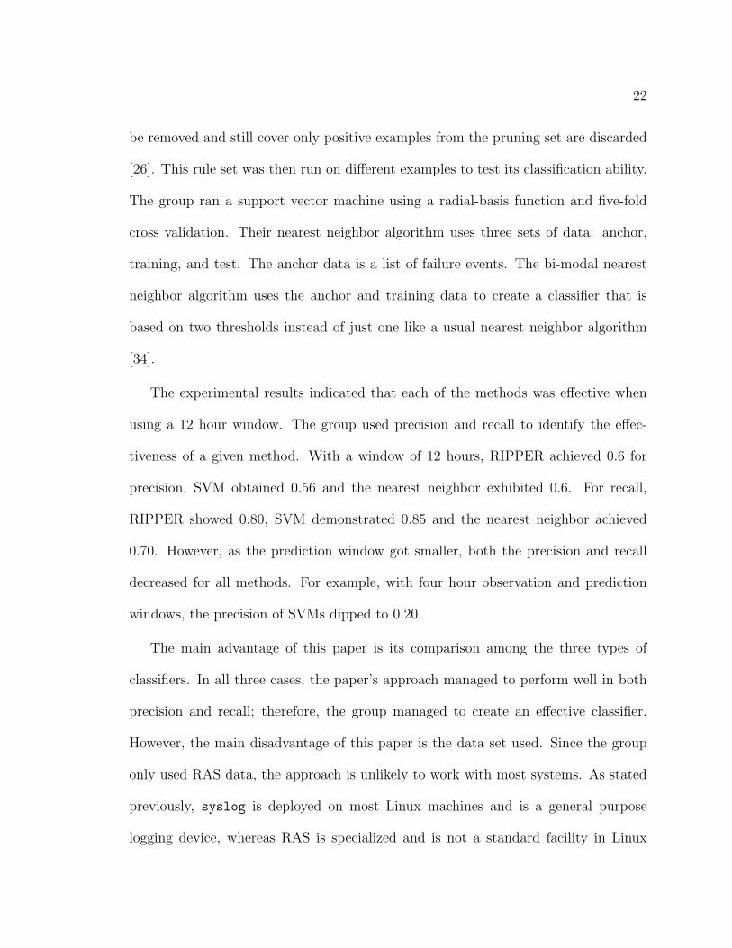
The experimental results indicated that each of the methods was effective when

using a 12 hour window. The group used precision and recall to identify the effec-

tiveness of a given method. With a window of 12 hours, RIPPER achieved 0.6 for

precision, SVM obtained 0.56 and the nearest neighbor exhibited 0.6. For recall,

RIPPER showed 0.80, SVM demonstrated 0.85 and the nearest neighbor achieved

0.70. However, as the prediction window got smaller, both the precision and recall

decreased for all methods. For example, with four hour observation and prediction

windows, the precision of SVMs dipped to 0.20.

The main advantage of this paper is its comparison among the three types of

classifiers. In all three cases, the paper’s approach managed to perform well in both

precision and recall; therefore, the group managed to create an effective classifier.

However, the main disadvantage of this paper is the data set used. Since the group

only used RAS data, the approach is unlikely to work with most systems. As stated

previously, syslog is deployed on most Linux machines and is a general purpose

logging device, whereas RAS is specialized and is not a standard facility in Linux

23

systems.

4.3 A Naive Bayesian Approach

Peter Broadwell also used Bayesian networks to predict hard disk failures [5]. Unlike

the work by Hammerly et al [15], Broadwell used event logs of the SCSI subsystem

instead of using snapshots of SMART data. This data set not only includes feedback

from the disk drives themselves, but also monitors the current effectiveness of the

SCSI cables themselves.

The setup for this study used a cluster made up of 17 storage nodes and 368

SCSI disks. The University of California, who maintained the cluster, kept most of

the kernel event logs generated during the course of their own unrelated experiment.

Only the kernel event logs from the storage nodes seem to have been kept.

The data set contained multiple types of failures. These failures included actual

disk failures, bad sectors on disks, errors which the system recovered from and SCSI

cable errors. To enlarge the data set, Broadwell clustered all of these errors into one

generic SCSI error class. As such, he tried to predict any sort of SCSI error, but

therefore was unable to determine specifically what kind of error was going to occur.

As a result, a system administrator would only know that something was going to

go wrong, but would not know what type of failure event would occur. On the other

hand, the research presented in this thesis focuses solely on disk failures, so a system

administrator would know that, specifically, a disk failure would occur. Broadwell

also analyzed the data at 24 hour time intervals, meaning that any failures would be

predicted at least 24 hours beforehand. However, the paper does not mention any

24

upper bound to this prediction window. All the user knows is that the disk will fail

in at least a day. The window method employed by this thesis can give a firmer time

of failure, such as a disk failing within two days.

Since the only two states that Broadwell cared about were whether the disks were

functioning normally or anomalously, he used two bins. One bin was used for normal

operation and the other for any sort of anomaly. Broadwell used journals kept by

system administratorss to figure out when failures occurred. He then correlated these

failure events with messages in the system’s event log. As a result, it is possible

that the system administrator’s records misclassified an event as a failure, the system

administrator was not aware of the failure until after the 24 hour window in which it

occurred had passed, or the system administrator completely missed a failure event.

Also, this is a very hands-on approach. It requires by-hand correlation, which will

not scale well to a large system, such as the data used in the experimental section of

this thesis. The approach presented in this thesis allows the user to avoid doing any

of this work by hand. After consulting the system administrators journal, Broadwell

found that over the period of the 11 months during which the data was collected,

there were 2 SCSI hard drive failures and 2 replaced SCSI cables.

Broadwell’s classification successfully identified anomalous patterns that lead to

all four of the failures in the data set. As such, his approach obtained 100% accuracy.

In addition, it identified one other pattern which did not correlate with any failure

noted by the system administrator. Broadwell attributes the success of his classifier

to the fact that it was very easy to generate a normal class and that drives which

were about to fail tended to operate in a sub-optimal state for multiple days before

25

actually failing.

4.4 Failure Trends

In 2007, Pinheiro, et al. examined both the characteristics of actual disk drive failures

and the possibility of building a model to predict drive failures using SMARTmessages

[24]. The main difference that sets this study apart from others on disk failures is the

size of the cluster from which the data was gathered. Also, while some studies, such

as the paper by Broadwell, use accelerated life tests to gather data, the team used

data from Google clusters based on actual use by the company.

The Google team did not use syslog data for their analysis. Instead, they built

their own database called the System Health Database which recorded the values of

various SMART data fields. This database keeps track of data from over one hundred

thousand disk drives.

The Google team based their prediction model on four of the SMART data pa-

rameters. The first was whether or not there had been any scan errors on a particular

disk. A single scan error indicated that a disk drive was 39 times more likely to fail

within 60 days than a disk with no scan errors. The next parameter was reallocation

count, which refers to a drive reassigning a sector number of a defective sector to a

sector from a set of spares. Just one reallocation meant that disk drive was 14 times

more likely to fail within 60 days than a disk with no reallocations. The third pa-

rameter was the number of offline reallocations. An offline reallocation occurred as a

result of the drive performing maintenance when not in use. As such, these realloca-

tions occur only as a result of errors that were not found during an I/O operation. A

26

single offline allocation correlated to a disk being 21 times more likely to fail within 60

days than a disk with no offline allocations. The final parameter was the probational

count, which indicates the number of sectors that the disk believes to be damaged.

A sector on probation may be returned to the set of good sectors if it does not fail

or have other errors after a certain number of accesses. Having even a single sector

on probation made a disk 16 times more likely to fail within 60 days than disks that

had no sectors on probation.

Unfortunately, the Google team also discovered that 56% of the disks which failed

during their test did not display any of these four errors previously. As such, any

model which is based only on these four counts to predict a failure will not be able

to predict more than half of the failures in a population. The paper concludes that,

since most of the disks did not display any warning signs before failing, using only

SMART data to predict failures is not sufficient. The lack of warning signs in the

SMART data provides motivation for the research in this thesis, which uses syslog

data that includes SMART messages. By using SMART data in conjunction with

syslog data, the approach presented in this thesis attempts to discern patterns of

activity across the whole system, which includes the disks themselves.

4.5 Statistical Approach to Failure Prediction

In Hard drive failure prediction using non-parametric statistical methods, Murray et

al. attempted to predict failures on a 369 disk collection [23]. All of the good disks

were obtained from a reliability test done by the manufacturers. Meanwhile, all of

the failed disks were returned to the manufacturer by end users. Obviously, since

27

one set was put through accelerated aging tests and the other endured actual use

from customers, the usage patterns between the two types of disks were different. It

is possible that any sort of modeling technique might be discovering the difference

between the two usage patterns and not the differences between failures and non-

failures. The type of data used was SMART data.

Murray compared the results of classification on the SMART data using three

methods: SVMs, clustering, and a rank-sum test. For the SVMs, each training set

was made up of 25% of the total good drives and 10% of the total failed drives. For

the unsupervised clustering, a cluster is created using only good drives. Then, a test

set was run. Any data point which did not fit the cluster of good drives was classified

as a failure.

The SVM approach had a failure detection rate of 17.5%. The paper does not

state whether the detection rate was based on accuracy, precision, recall, or some

other metric. When using a combination of of features (the previous test only used

one feature), the rank-sum test can predict 43.1% of failures.

This paper has two main disadvantages. The first disadvantage is that the group

solely used SMART data, which Pinheiro et al. have shown is insufficient for predic-

tions. Second, the disk failures were those reported by users. Therefore, it is possible

that users returned disks which had not actually failed. Users probably had different

definitions of what constituted a disk failure. In the case of the syslog and SMART

data used by this thesis, all disk failures were reported by the same facility, and there-

fore were all based on some standardized criteria. Also, all of the disks used in this

thesis experienced ”normal wear and tear,” as opposed to undergoing accelerated life

28

tests to simulate normal behavior.

4.6 System Board Failures

Doug Turnbull used a method similar to the method presented in this thesis [33].

Instead of predicting hard drive failure, however, they predicted system board failure

using a collection of 18 system boards on only one system and logs of their activities

[33]. The log was broken up into sensor and potential failure windows. If a failure

actually occurred during the failure window, then the features in the sensor window

were labelled as positive and negative otherwise.

Similar to the approach in this thesis, Turnbull combined both raw feature vectors

and aggregate feature vectors. Each of the system boards had 18 sensors and a sample

of each was taken once per minute. As such, a raw feature vector contained 18 × n

samples, where n is the number of entries during a certain sensor window. A summary

vector was a bit more complex, as it contained 72 features representing statistics like

mean and standard deviation.

The data was collected over five months and saw 65 system board failures. Turn-

bull randomly selected 65 non-failure feature sets and performed 10-fold cross-validation.

Using 48 features, Turnbull was able to get a 0.87 true positive rate. This paper is

significant because it shows that event predictions can be made successfully using

event logs. However, the paper uses event logs kept by system boards and not event

logs kept by the operating system, such as syslog. This paper also differs from the

research presented in this thesis in that this thesis focuses on the prediction of disk

failures as opposed to board failures.

29

4.7 Summary

In conclusion, many different methods have been attempted to predict various types

of failures. Hammerly et al. [15] used a naive Bayesian classifier on SMART data

and managed to predict disk failures that would occur in the next 48 hours with 52%

accuracy. A team from IBM [20] used data from a specialized logging system on its

BlueGene cluster. The team then performed predictions using a rule based classifier,

an SVM, and a nearest neighbor algorithm. While the team achieved high accuracy,

its data set may be too specialized to be of use by the general public. Peter Broadwell

[5] used a supervised Bayesian approach to predict SCSI cable failures. While he was

able to create an effective prediction method (he was able to predict all of the failures

in his data set), the approach presented in the paper is not scalable. Pinheiro et al [24]

concluded that SMART data is insufficient for creating a successful prediction model.

Murray et al [23] compared the effectiveness of SVMs, clustering, and a rank-sum

test for failure predictions using SMART data. Finally, Turnbull et al [33] proposed

an approach similar to the one presented in this thesis. However, Turnbull focused

on predicting system board failures instead of disk failures.

Chapter 5: New Spectrum-Kernel Based

Methods for Failure Predictions

As described in Chapter 3, predicting disk failures can be modeled as a classifi-

cation problem. The representation stage of the classification problem requires that

features be extracted from the data set so that a classifier can be applied to the data.

This chapter discusses the method employed by the research detailed in this thesis

to extract features from syslog data as well as how this data is transformed for use

with classification methods.

5.1 Sequences

As described by Pinheiro et al., single messages are not sufficient for predicting

failure[24]. However, examining sequences of messages may be a more effective means

of failure predictions. The messages in a syslog file are stored in the same order in

which they were posted. Since the first message in a file correlates to the first message

received, the second message in the file to the second received, and so forth, all of

the data in syslog is stored sequentially. Therefore, it is possible to turn the failure

classification problem into what Dietterech terms a sequential classification problem

[10].

To better illustrate the sequential classification problem, Dietterech uses the ex-

ample of handwriting recognition. Consider an English word written by a human,

30

31

such as the word “crouching.” The normal classification problem would attempt to

discern each letter in isolation. A simple example of an error this approach might

make is mistaking the“g” at the end of “crouching” for a “q.” However, using a se-

quential approach to the problem, a classifier might exploit the fact that it has seen

many sequences of ’ing’ before while it has seen fewer sequences of “inq”, especially

at the end of a word. As such, the sequential classification approach will leverage

the fact that “ing” is a common sequence of letters in the English language, whereas

“inq” is not. Similarly, a syslog message which reports disk temperature may be

innocuous by itself, but that same message followed by a flurry of other disk-related

events could provide an indication that the disk is failing.

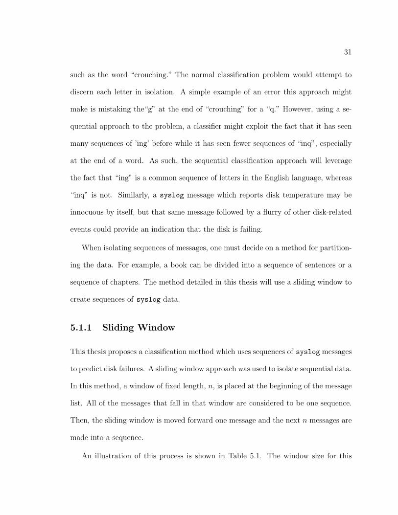
When isolating sequences of messages, one must decide on a method for partition-

ing the data. For example, a book can be divided into a sequence of sentences or a

sequence of chapters. The method detailed in this thesis will use a sliding window to

create sequences of syslog data.

5.1.1 Sliding Window

This thesis proposes a classification method which uses sequences of syslog messages

to predict disk failures. A sliding window approach was used to isolate sequential data.

In this method, a window of fixed length, n, is placed at the beginning of the message

list. All of the messages that fall in that window are considered to be one sequence.

Then, the sliding window is moved forward one message and the next n messages are

made into a sequence.

An illustration of this process is shown in Table 5.1. The window size for this

32

example is 3. The first sequence would be ABB. Then, the window moves one place

to the right to start on the B and isolates the sequence BBA. The rest of the sequences

are shown in Table 5.2. Once determined, the spectrum kernel approach is applied

to these sequences.

A B B A C B

Table 5.1: A list of letters

Letter SequencesABBBBABACACB

Table 5.2: Letter sequences using a sliding window of length 3

5.1.2 Spectrum Kernel

The spectrum kernel technique was devised by Leslie et al. [19] to leverage sequences

of data for use with a classifier. The spectrum kernel can be used on any input

space X made up of finite length sequences from an alphabet A. For any k ≥ 1,

the k-spectrum of a given input sequence is defined as all of the subsequences of

length k that the sequence contains. In the handwriting problem described above,

A is the 27 letter English alphabet. Say that the sequence being examined is the

word “crouching”. If k = 3, then each 3 letter subsequence is found. For example,

the first subsequence is “cro”, the next “rou”, and so forth. The sequence number

being computed is t and the previous sequence number is t − 1. Given a sequence

length k, an alphabet size b and a single member of the alphabet, e, the spectrum

33

f(1) = mod(3× 1, 33) + 0 = 3f(2) = mod(3× 3, 33) + 1 = 10f(3) = mod(3× 1, 33) + 2 = 5

Figure 5.1: An example computation of sequence numbers

kernel representation of a given sequence can be obtained using Equation 5.1 [32].

The equation must be applied for each letter in the input.

f(t) = mod(b ∗ f(t− 1), bk) + e (5.1)

For example, consider Table 5.3, which assigns a numerical value to each letter in

a three letter alphabet. Table 5.4 shows the sequences and sequence numbers for the

string “BABC” where the sequence length is 3, assuming processing moves from left

to right. To compute the first sequence number, start with “B”. Since the numerical

encoding of “B” is 1, f(0) = 1. The following terms are found by using Equation

5.1. The results of these calculations are shown in Figure 5.1. The sequence number

for the sequence “BA” is not shown in Table 5.4 because sequence numbers are not

recorded until the first k letters are seen. Calculating the sequence number of “BA” is

an intermediate step in computing the sequence number of the first 3 letter sequence,

“BAB.”

Letter EncodingA 0B 1C 2

Table 5.3: Numerical assignments for letters

The above example details the method for assigning sequence numbers to an

34

Letter Sequence Sequence NumberB 1A 10B 101 10C 012 5

Table 5.4: Sequence numbers where k = 3

ordered list of values. The same approach will be used to create sequence numbers

for syslog messages. Specifically, this thesis examines sequences based on the syslog

tag number and message fields.

5.2 Tag Based Features

Consider the tag numbers that occur within a message window. The order in which

these messages appear forms a list of tag numbers. From this list of tag numbers,

one can create a feature vector which combines two types of features: a count of the

number of times each tag number and sequence number appears in a window. An

example of determining the tag number count is show in Tables 5.5 and 5.6.

Time Tag Number1172744793 1481172744794 1481172744799 1581172744810 401172744922 1581172744940 1881172744944 148

Table 5.5: The raw tag numbers

As described in the previous section, each ordered sequence of tags in the file is

given a number based on two factors. The first factor is the length of the sequence

35

Feature Vector Meaning40:1 Tag value 40 occurred once148:3 Tag value 148 occurred three times158:2 Tag value 158 occurred twice188:1 Tag value 188 occurred once

Table 5.6: The resulting feature vectors

to be considered, which corresponds to k in Equation 5.1. If k = 4, then only the

previous four tag numbers are considered when computing a sequence number. The

other factor is the alphabet of available values, called b in Equation 5.1. When

processing starts, the size of the alphabet is the number of unique tag numbers in

syslog, which, in this example, is 189. Using sequences of length 5, the list of possible

features is 1895, which equates to over 241 billion unique combinations. Generally, not

all possible sequences appear in the input, so the actual number of features is much

smaller. Nevertheless, computing sequence numbers for all of these combinations

will take an excessively long time. Therefore, either the sequence length or the size

of the alphabet must be reduced. Since the expression is exponential in terms of

the alphabet size, the available number of sequences can shrink more dramatically

when reducing the alphabet size than it does when reducing the sequence length. For

example, if the original alphabet consists of 189 values, then using sequences of length

4 results in a feature space of over 1.2 billion features. Reducing the sequence length

to 3 shrinks the feature space to 6.75 million features. However, using sequences of

length 4 and changing the alphabet size from 189 values to 20 values results in a

feature space of 160,000 features.

The alphabet size can be reduced through a non-linear mapping of multiple entries

36

in the original alphabet to a single value in the reduced alphabet. For example, in

the approach proposed in this thesis, the size of the alphabet is reduced to size 3.

Each tag number is assigned an importance number of either 0, 1, or 2. Messages

of high criticality, and therefore a lower tag number, are assigned 0. Messages of

medium criticality are assigned a 1 and messages of low criticality are assigned a 2.

Tag numbers which are less than or equal to a 10 are considered to be high priority.

Tag numbers between 11 and 140 are considered medium priority and tag numbers

above 140 are considered low priority. The size of the reduced alphabet and cutoff

values are determined by examining the distribution of tag numbers as seen in Figure

2.1. After reducing the alphabet size, one can assign the sequence numbers using

Equation 5.1.

Consider the message sequence in Table 5.7. The left column shows the original tag

number. The middle column contains the tag message’s value in the reduced alphabet.

The rightmost column holds the sequence number determined by the equation. The

reason there are ten messages, but only six sequence numbers is that sequence numbers

are not fully computed until the first sequence of length five occurs. While each

sequence can appear multiple times, each occurrence of this sequence is assigned the

same number. For example, the sequence “22122” appears twice in Table 5.7 and

is assigned a sequence number of 233 both times. Once the sequence numbers are

computed, a count of the number of times each sequence number appears in the

window is added to the feature vector.

37

Tag Translated Sequence148 2148 2158 240 1158 2 239188 2 233188 2 21588 1 160158 2 239188 2 233

Table 5.7: An example of tag-based sequence numbers

5.2.1 Tags With Timing Information

Timing information is another feature that may help improve failure predictions. In

this case, the timestamp of each message was also retained. The purpose of examining

timing information is to discern whether or not there is some pattern in how quickly

messages are posted when a failure is imminent. For example, perhaps a dramatic

increase in the rate of messages indicates that a failure is likely. During the creation of

the sequence numbers, the difference between time of the first message in the sequence

and the time of the last message in the sequence is recorded. Doing so provides an

indication of how quickly or how slowly those messages were posted. The differences

in time are recorded in the same format as the tag and sequence numbers.

Consider the list of tag numbers in Table 5.5 again. This table also contains the

timestamp of each message. The difference between the first and last message of each

sequence is show in Table 5.8 and the resultant feature vectors are shown in Table

5.9. The tables each assume a sequence length of 3. The first two rows of Table

5.8 do not have any numbers listed in the difference column because the difference is

38

not recorded until the first sequence has passed. Once the time count is performed,

these counts are also added to the feature vector containing tag number counts and

sequence number counts.

Time Difference Tag Number- 148- 1486 15816 40123 158130 18822 148

Table 5.8: Time Difference and Tag numbers

Time Count6:116:122:1123:1130:1

Table 5.9: The feature vectors the result from timing information

5.3 Message Based Approaches

The myriad possible syslog configurations allow for a set up in which tag numbers

are not present [21]. One thing an administrator is unlikely to remove is the message

field itself. A string is defined as any space-delineated collection of characters in the

message field. For example, a string can be an English word, an IP address, or a

number. Tag numbers are not factored into this approach, as seen in Tables 5.12 and

5.13. The goal of this method is similar to the tag-based experiments: to discover

39

some pattern of actual strings which will allow for failure prediction.

The first approach to encoding strings is very similar to the use of tag numbers.

In this case, each string is given a unique number. An example of this process is

shown in Tables 5.10 to 5.12. Table 5.10 contains the original syslog messages.

Table 5.11 shows the assignment of numbers to each string. Finally, Table 5.12 shows

the translated syslog message with strings replaced by their numbers. The syslog

data is then transformed into a list of strings, shown in Table 5.13, in which a given

sequence could span multiple syslog messages. For example, consider Table 5.10. If

the sliding window is of length 4, then the first sequence includes the three strings

from the first message and the first string of the second message. Equation 5.1 is

applied to obtain a list of sequence numbers representing keystring sequences and a

frequency count of the sequence numbers is then recorded.

Host Facility Level Tag Time Message

node52 local4 info 166 1172744793 xinetd 905 START

node52 kern alert 5 1172746564 kernel raid5: Disk failure on sde1

node52 kern info 6 1172746564 kernel md: updating md9 RAID

Table 5.10: The original messages

Unfortunately, the list of possible strings can be quite large. For example, the

syslog data set used in this thesis contains over 2 billion unique strings, despite the

fact that the English language only consists of about 1 million words [29]. Consider

a message which posts the temperature of a disk drive. Even if the temperature

only fluctuated by ten degrees across all log files, those ten values (assuming the

message only posts integer values) are assigned unique identifiers in the alphabet.

This alphabet results in a massive feature space. For example, when using sequences

of length 3, the resulting feature space contains over 8× 1027 unique sequences. This

40

Word Numberxinetd 0905 1START 2kernel 3raid5: 4Disk 5failure 6on 7sde1 8md: 9updating 10md9 11RAID 12

Table 5.11: Translation from a word to its unique number

Host Facility Level Tag Time Message

node52 local4 info 166 1172744793 0 1 2

node52 kern alert 5 1172746564 3 4 5 6 7 8

node52 kern info 6 1172746564 3 9 10 11 12

Table 5.12: The translated messages

space is far too large to classify on, as it far exceeds the number of integers that a

computer can represent. Another concern is that the alphabet is determined after

all of the data has been collected. Were this to be deployed in an actual system

while syslog data is still being gathered, there is the chance that a message that

does appear in the data set will eventually be posted and a string that has not been

seen before will be used. As a result, the alphabet size will increase and the sequence

numbers determined using Equation 5.1 will need to be recomputed. Since all of the

sequence numbers will change, a user will have to retrain the model. Some attempt

at reducing the alphabet to a finite size is required. By ensuring that the alphabet

size remains fixed, sequence numbers never have to be recomputed, which means a

41

new model does not need to be created. The use of tag numbers does not have this

problem. For example, if the possible values for tag numbers is exactly 189, then it

will always remain 189. As previously described, the approach proposed above will

always be mapped to exactly 3 values.

5.3.1 Using Keystrings as Features

Only Keystrings

In an effort to reduce the alphabet size (number of strings), it is possible to isolate

only the strings that the classifier finds useful in creating a model. To do this, the

classifier is trained on the entire data set, using only the number of times each string

appears. Once the classifier builds a model of the data, the feature space is examined

to determine the most important strings. For example, a given list might contain 54

strings. Any string which the classifier finds useful will henceforth be referred to as a

keystring.

Now that there is a list of the most important strings, the simple solution is to

use only these strings. These strings are used to create the message list. A count

of each string is used as well as a count of each sequence of strings. The smaller

alphabet allows for the use of sequences up to length 4. When building a sequence

number, message boundaries are ignored. For example, consider Table 5.13 through

Table 5.16. Table 5.13 contains a list of three syslog messages. In Table 5.14, the list

of keystrings is presented. Table 5.15 illustrates the list of keystrings that results by

applying the dictionary in Table 5.14 to the syslog messages in Table 5.13. Assuming

a sliding window of size two, the first window will contain the first two lines in Table

42

5.16. In the original syslog file, these two keystrings were in two separate messages.

Therefore, the resultant list can be considered to be a stream of keystrings.

Host Facility Level Tag Time Message

node52 local4 info 166 1172744793 xinetd 905 START: shell pid=16548 from=198.129.149.213

node52 kern alert 5 1172746564 kernel raid5: Disk failure on sde1disabling device.

node52 kern info 6 1172746564 kernel md: updating md9 RAID superblock on device

Table 5.13: The original messages

String Numberkernel 0md9 1

Table 5.14: A list of example keystrings

Time Message11727447931172746564 01172746564 0 1

Table 5.15: The converted messages from Table 5.13 using the keystrings in Table5.14

Keystring001

Table 5.16: The resulting keystring list from Table 5.15

Since only the keystrings in a given message are retained, it is possible that all of

the strings in a given message will be removed from the message list. In this case,

the timestamp of syslog events with empty message fields is retained to allow for

the use of timing information. Therefore, these messages are still considered when

creating a message window. Consider the messages in Table 5.15.

43

Many keystrings may represent similar items. For example, each computer may

have a unique ID number. While each of these keystrings is unique, they all fall

under the general label of an ID number. In the interest of reducing the alphabet

further, strings are grouped into general types, such as computer ID number, and

a number is assigned to each type. This thesis compares the effectiveness of the

classifier when using the original keystring dictionary and the more general, reduced

keystring dictionary.

5.3.2 Keystrings With Timing Information

Timing information can also be included when using the keystring approach. The

keystring methods described above retain the message timestamp. As with the tag

approach, a count is taken of the differences between the time at which the first

message in a sequence is posted and that of the final message in a sequence. These

counts are then added as new features to the number of times each keystring is seen

and the number of times that each sequence of keystrings appears. As with tags, the

timing information is added to discern whether or not the rate at which messages are

posted relates in any way to the likelihood of a failure in the near future.

5.4 Combining Tag-based and Keystring-based

Approaches

It is possible to combine the tag number and keystring approaches. The motivation

behind this approach is that the combination of the two approaches might allow for

even higher accuracy. The best of the tag combinations is combined with the best

44

of the string combinations. The same keystring dictionary and sequence length for

keystrings is used as is used in the best performing keystring experiment. Similarly,

the most effective sequence length for tags is used to encode the tags. For example,

suppose the keystrings perform best with sequences of length 3, but tags perform

best with sequences of length 6. For example, int the experimental results chapter,

keystring sequences of length 4 are computed and tag sequences of length 5 are com-

puted. The final feature vector includes tag count, tag sequence count, keystring

count, keystring sequence count, and time information.

Chapter 6: Support Vector Machines

The goal of this thesis is to develop a method for predicting disk failures. Each

disk can be separated into one of two classes: a disk which failed or a disk which

did not fail. Classification methods can be used to isolate patterns that indicate

disks which fail. As discussed in Chapter 3, a given classification algorithm can use

unsupervised, supervised, or semi-supervised learning approaches. The classification

method used in this thesis is a supervised learning method called a support vector

machine, or SVM.

6.1 The Data

An SVM is a classification method that takes a set of labeled training examples of

the form

(y1, x1), (y2, x2), ..., (yi, xi), yj ∈ {−1, 1}, xj ∈ Rn. (6.1)

The y term must be either a positive or negative 1, while the x term is a vector

of real numbers. A positive 1 for y provides the example label indicating that the

corresponding x represents an example that is of a given class, while a negative 1

indicates that the x is not part of a given class.

6.2 Optimal Hyperplane

Using an input set of labeled data points, the SVM attempts to find an optimal

hyperplane to separate the data. Consider Figure 6.1, which provides an illustration

45

46

Figure 6.1: An illustration of the optimal 2-D hyperplane

of the optimal hyperplane between the class of circles and the class of crosses. There

are an infinite number of hyperplanes between the classes. The optimal hyperplane

is the plane which maximizes the distance between the two classes. In the case of the

figure, the optimal hyperplane is represented by the solid line.

To calculate the optimal hyperplane, one finds the planes that separate the data

which are located closest to each class. In Figure 6.1, the hyperplanes which lay as

near as possible to each class are represented by dashed lines. One of these hyperplanes

passes through the two circles which are closest to the class of crosses. This hyperplane

still separates the two classes, because all of the circles are either on or above and

to the left of this hyperplane, while all crosses are below and to the right of this

hyperplane. Similarly, the other dashed line passes through the two crosses which

are nearest to the class of circles. Since these hyperplanes are defined by the points

47

closest to the optimal hyperplane, only these few examples are needed to calculate

the optimal hyperplane. These data points are called support vectors. The optimal

hyperplane is defined using Equation 6.2 [8], where b is a scalar value and w is a

vector of weights which defines the optimal hyperplane [18].

(w · x) + b = 0 (6.2)

Figure 6.1 shows a case in which the classes are separable in the two dimensional

plane. However, it is possible that a data set will be impossible to separate in this

plane, as in Figure 6.2. In this case, a method [8] exists for transforming the data

into a higher dimensional space in which a hyperplane can be constructed. Figure

6.2 and 6.3 provides an example of this process. The data in the graph on the left

cannot be separated in two dimensions, but it can be separated in three dimensional

space. The data can be transformed into whatever dimension is necessary to separate

the data, not just two or three dimensions. This process is discussed in more detail

in Section 6.3.

Figure 6.2: An example where the data must be mapped to higher dimensions

Whether or not a given feature is classified as being part of a class depends on

48

the equivalency shown in Equations 6.3 and 6.4 [8].

(w · xi) + b ≥ 1, yi = 1 (6.3)

(w · xi) + b ≤ −1, yi = −1 (6.4)

In Equations 6.3 and 6.4, w is a vector of feature weights, x is a given feature

vector, and b is a scalar threshold.

Ideally, the number of support vectors should be small. The probability of an error

occurring on a test classification is bounded by the number of support vectors com-

pared to the overall number of feature vectors, as shown in Equation 6.5. E[Pr(error)]

is the expected error of the model when applied to a test set. E[number of support vectors]

is the expected number of support vectors for a given number of training vectors.

E[Pr(error)] =E[number of support vectors]

number of training vectors(6.5)

Equation 6.4 provides a measure of generalizability for a given model. While

the hyperplane may work very well for a given training set, if the number of support

vectors is high, then the model will be less generalizable to test vectors. The equation

provides an upper bound for the number of errors that the classifier is expected to

commit when classifying on a test set.

6.3 SVM Kernels

All of the above equations deal with creating a hyperplane using the n-dimensional

input space. However, to perform the SVM evaluation, these vectors may need to be

transformed into a larger N -dimensional feature space using the equivalence:

φ : Rn → RN . (6.6)

49

This equivalence is non-linear. This motivation behind performing this transform

is that computing an optimal hyperplane in the input space is not always possible. As

an alternative, the vectors in the input space are transformed to a higher dimensional

space in which the determination of the hyperplane can occur. Converting to a higher

dimensional space requires the computation of the following dot product:

k(x, y) = φ(x) · φ(y). (6.7)

As mentioned by Cortes and Vapnik, this task is computationally intensive. They also

note that previous work [4] has indicated that, when constructing a decision function,

the order of operations can be interchanged. As a result, while a set of vectors may

only be linearly separable in a higher dimensional space, the computations may be

performed in the input space. The transformation function, k, is called a kernel.

6.3.1 Linear Kernel

The majority of the tests done in this thesis are performed using the linear kernel.

Assuming the training vectors are linearly separable in input space, then they are

not mapped to a higher dimensional space. Therefore, the weights assigned to each

vector can be used to determine which features are the most useful for separating two

classes [32].

It is possible that misclassifying one or more training examples will allow for a

better overall separation of the two classes. The linear kernel allows the user to adjust

the number of training examples which may be mislabeled. This tradeoff is defined

by the C value. The C defines the penalty incurred for each mislabeled training

example. Essentially, the SVM tries to maximize the distance between two classes.

50

If the distance between two classes can be increased by more than the C value if one

of the training examples is misclassified, then a hyperplane which misclassifies that

example is used [6]. So, for example, a given training example may be misclassified if

the cost penalty is 1. However, if the cost penalty is increased to 100, so that the cost

of misclassifying the example exceeds the benefit, then the hyperplane which classes

that example correctly is used.

6.3.2 Polynomial Kernel

The polynomial kernel allows the SVM to use polynomials with degrees greater than 1

to separate the data. For example, in a two dimensional input space, the linear kernel

determines the straight line which best separates the two classes. This is equivalent to

using a polynomial kernel of degree 1. The degree of the polynomial can be increased

to any integer value. So, for example, if the degree of the polynomial is 2, then the

SVM will use a quadratic line to separate the classes [34]. In SVM-Light, the degree

of the polynomial is determined by the user-defined D value.

6.3.3 Radial Basis Function

The radial basis function creates a model by using a process similar to clustering.

During training, each example is considered to be the center of a cluster. The gamma

value, referred to as the G value, defines the size of each cluster. The resulting clusters

then undergo a linear combination to create two clusters which separate the classes

[34].

51

6.4 Theoretical Complexity

While the classical SVM method has a time complexity of O(n3) where n is the size

of the training set [31], various improvements are possible. Thorsten Joachims has

shown that it is possible to train a linear SVM in O(sn) time, where s is the number

of support vectors and n is the number of training examples [17].

The space complexity during the training step is O(n2) where n is the number of

training examples. This growth is a result of the final training step, which requires

k(k+1)2

dot products, where k is the number of support vectors. If the problem is

linearly separable in the input space, it has been shown that the number of support

vectors grows less than linearly with respect to the number of training examples [3].

Chapter 7: Experimental Results

7.1 Introduction

This chapter describes the specific steps performed on the input data to extract

sequence data and train the classifier. The data set used is syslog data collected

over a sixth month period from a 1024 node Linux cluster maintained at the Pacific

Northwest National Laboratory. On average, there are 78 syslog messages posted

for a given node on a given day. The syslog data contains messages reported by the

SMART disk monitoring facility. As such, the data contains some messages which

indicate the status of the hard drives on a given node, in addition to other information

about the events on the node.

This approach uses SVMs to train on and classify the data using the feature space

described in Chapter 5. The particular SVM implementation used is SVM-Light,

coded by Thorsten Joachims [16]. SVM-Light was chosen for many reasons. First, it

is open source, which allows for the possibility of modification. Also, while binaries

are provided for Windows, Solaris, and Linux, the fact that it is open source allows for

the program to be compiled on other operating systems, such as OS X, which furthers

the goal of this research to be generalizable. SVM-Light also provides a variety of

kernels, specifically the linear, polynomial, and radial basis function kernels. Finally,

SVM-Light employs an efficient optimization algorithm which allows it to train a

model very quickly.

52

53

For a given experiment, a window is created of messages preceding the failure.

Features, specifically sequences of events, are created from these blocks of messages.

The resulting features are then used as input to SVM-Light, which builds a model

for classifying data as representative of a disk failure or not representative of a disk

failure. This model is then applied to a test set to determine the effectiveness of the

model.

All experiments are performed using hold out and 10-fold cross validation. Hold

out means that for both the training and testing stages, an equal number of failure

and non-failure examples are in the data set [34]. When using 10-fold cross validation,

the data is broken up into ten sets of equal size. The classifier is then trained on nine

of these sets and tested on the final set. A different test set is then chosen from the

ten groups, while the previous test set is added to the training set, so each of the ten

slices eventually is used for testing [34].

For example, suppose there are 40 valid disk failures in the data set. Since these

experiments use hold out, 40 random examples of disks which did not fail are selected.

The resulting 80 event data set is broken up into ten equal groups, each of size 8.

Each group contains 4 failure events and 4 non-failure events. SVM-Light trains on

nine of the groups, or 72 message sets, and is tested on the remaining 8. Then, a

different group of 8 messages is used as the test set while the original group of 8 is

returned to the training set. After all 10 folds are completed, each message has been

in the test set one time. Each experiment was repeated 100 times and the results

were averaged.

Accuracy, precision, and recall are used to measure the performance of a given

54

method. Accuracy is the total number of correct predictions divided by the total

number of inputs. Therefore, accuracy measures the percentage of the predictions,

either negative or positive, that were correct. Precision is determined by the num-

ber of true positive predictions over the total number of positive predictions. This

metric measures how many of the nodes which are predicted to experience a disk

failure actually do experience a failure. Maximizing precision is desirable, because

a lower precision means that more disk drives will be replaced than actually failed.

Each working disk that is replaced represents both an unnecessary monetary and a

performance cost. Finally, recall is the number of true positive predictions over the

total number of positive inputs. This metric measures how many of the actual disk

failures are predicted. A higher recall is good because that means more of the disk

failures are predicted, which means the effect of each failure can be mitigated.

7.2 Tag Numbers

7.2.1 Preprocessing

To simplify later processing, each log file is opened and the timestamp and tag number

of each message in the log is written to a new file. As each line is parsed, it is also

determined whether or not the given message is a disk failure message. If the message

is not a failure, a -1 is added to the end of the line. If the message is a failure, a +1

is added to the given line. For example, consider the following two tables. Table 7.1

shows three syslog messages. The second message in the sequence is a disk failure

message. Table 7.2 shows the output of the parsing process. The first column contains

the time the message was posted while the second column indicates the tag number

55

and the final column shows whether or not the corresponding syslog message was a

disk failure.

Host Facility Level Tag Time Message

node52 local4 info 166 1172744793 xinetd 905 START: shell pid=16548 from=198.129.149.213

node52 kern alert 5 1172746564 kernel raid5: Disk failure on sde1 disabling device.

node52 kern info 6 1172746564 kernel md: updating md9 RAID superblock on device

Table 7.1: The original messages

Time Tag Failure1172744793 166 -11172746564 5 +11172746564 6 -1

Table 7.2: The reduced messages

The files are then sorted into a group of files which contain failures and a group

in which no failures are seen. Each file is examined again. If, at any point in the file,

the last field of a line is a +1, that file is moved to a specific folder. If no line ends in

+1, then that file is moved to a different folder.

Next, the files are broken up into message windows. The size of the message

window specifies the number of messages to isolate prior to a failure. For example,

if the window size is 500, then a new file is created which contains the 500 messages

immediately preceding the failure message. However, if there are not enough messages

before the failure, then that window of messages is not used. For example, if the

window size is 500, but the failure message occurs on the third line of a file, then the

failure on line 3 is not used. Also, if a given failure comes within twenty four hours

of a previous failure, then the failure is removed from the data set. The original data

set contains over 100 disk failures. After removing the above failures from the data

set, 41 disk failures remain. The reduction is so significant because often one disk

56

failure is followed very closely by two or three more failures on the same node. These

failures are thrown out to keep any patterns or events which lead to the first failure

from affecting predictions for subsequent failures.

The process is slightly different for files in which there are no failures. The number

of messages in each file is counted. If there are fewer lines in a given syslog file than

are required by the window size, then the syslog file is discarded. Otherwise, a

random start line is chosen in the file, then a message window of the designated size

is created starting at that message. If the number of messages between the start line

and the end line is fewer than the number of lines required by the window size, then

a new start line is randomly chosen until the desired window size can be created.

Once all of the message windows are created, they have to be trimmed one final

time. To simulate lead time before a failure, a specified number of messages at the

end of the window is removed. By deleting messages at the end of the file, there is

a gap between the end of the message list and the event to be predicted. This gap

simulates some amount of lead time when making the prediction. As an example,

consider a window size of 1,200 messages. This window corresponds to about 15 days

of syslog messages for the syslog files used in these experiments. If the window

is then trimmed by 200 messages, there are 1,000 messages left to classify on. The

remaining 1,000 messages will be referred to as a message block. By eliminating the

last 200 messages, there is a gap of a little over two days between the final message

in the block and the failure or non-failure. Therefore, if a disk is predicted to fail, it

is predicted to fail in about two days.

Each file now consists of a list of tag numbers. It is time to create a list of features

57

for each failure or non-failure. The same process is performed for both types of files

with one difference: a failure occurrence is labelled with a +1 at the start of the list of

feature vectors and a list of feature vectors which does not lead to a failure is labelled

with a -1. SVM Light uses these labels to determine whether or not the given feature

list is indicative of a failure or of a non-failure.

A Comparison of SVM Kernels Using Tag-Based Features

The following experiments use a window of 1,200 messages and a lead time of 200

messages. The features used are a count of the number of times each tag number

appears in a file and the number of times each sequence of length five appears in the

file [13]. These experiments examine the effectiveness of the different types of kernels

supported by SVM-Light in predicting disk failures. The kernels compared are the

linear kernel, polynomial kernel, and radial basis function kernel. SVM-Light allows

the user to set certain parameters for each of the kernels. The next few experiments

also examine the effectiveness of altering these parameters. The purpose of this series

of experiments is to determine both the most effective kernel for this classification

problem and the optimal value of the parameters for each kernel.

Table 7.3 lists the accuracy, precision, and recall of the linear kernel using the

window size, lead time, and sequence length described above. The table indicates

the effect of changing the C value for the linear kernel. The C value is defined as

the trade off between the training error and the optimal margin. In other words,

it allows for some training examples to be mislabeled if that will allow for a more

effective hyperplane overall [16]. Each test is performed using hold out and 10-fold

cross validation. Tests are repeated 100 times and the results are averaged. A cost

58

penalty of .75 for each misclassified example provides the optimal combination of

precision and recall. Reducing the C from 1 allows for more labels to be misclassified,

but decreasing C past .75 means that the cost for each misclassified example is so low

that too many examples are misclassified to provide any benefit.

C Value Accuracy Precision RecallDefault 75.3831 81.5504 66.8673.25 72.9999 75.6003 74.6672.50 72.8337 75.9006 70.334.75 76.3326 78.8672 75.00081 74.8329 79.5505 71.6675

Table 7.3: The Effect of C Value on Linear Kernel Performance.

Table 7.4 shows the effectiveness of the polynomial kernel. When using the poly-

nomial kernel, one can alter the degree of the polynomial used to separate the classes.

For example, using a D value of 1 means that SVM-Light will try to use a straight

line to separate the classes. Changing the D value to 2 allows SVM-Light to use a

quadratic function to separate the classes.

D Value Accuracy Precision Recall1 76.0 82.6338 73.66782 75.9999 80.2504 76.66753 50 0 0

Table 7.4: The Effect of the D Value on Polynomial Kernel Performance.

The final kernel tested is the radial basis function, or RBF. The results of adjusting

the gamma value of the radial basis function are shown in Table 7.5. The gamma

value adjusts the width of each RBF.

By examining Table 7.3, Table 7.4 and Table 7.5, it is apparent that the radial basis

function approach performs similarly to the polynomial and linear kernels with respect

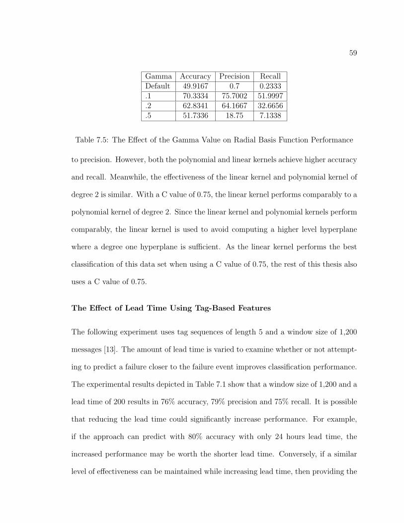
59

Gamma Accuracy Precision RecallDefault 49.9167 0.7 0.2333.1 70.3334 75.7002 51.9997.2 62.8341 64.1667 32.6656.5 51.7336 18.75 7.1338

Table 7.5: The Effect of the Gamma Value on Radial Basis Function Performance

to precision. However, both the polynomial and linear kernels achieve higher accuracy

and recall. Meanwhile, the effectiveness of the linear kernel and polynomial kernel of

degree 2 is similar. With a C value of 0.75, the linear kernel performs comparably to a

polynomial kernel of degree 2. Since the linear kernel and polynomial kernels perform

comparably, the linear kernel is used to avoid computing a higher level hyperplane

where a degree one hyperplane is sufficient. As the linear kernel performs the best

classification of this data set when using a C value of 0.75, the rest of this thesis also

uses a C value of 0.75.

The Effect of Lead Time Using Tag-Based Features

The following experiment uses tag sequences of length 5 and a window size of 1,200

messages [13]. The amount of lead time is varied to examine whether or not attempt-

ing to predict a failure closer to the failure event improves classification performance.

The experimental results depicted in Table 7.1 show that a window size of 1,200 and a

lead time of 200 results in 76% accuracy, 79% precision and 75% recall. It is possible

that reducing the lead time could significantly increase performance. For example,

if the approach can predict with 80% accuracy with only 24 hours lead time, the

increased performance may be worth the shorter lead time. Conversely, if a similar

level of effectiveness can be maintained while increasing lead time, then providing the

60

0 100 200 300 400 500 60050

55

60

65

70

75

80

85

90

95

100

Lead Time

Per

cent

age

The Effect of Lead Time On SVM Performance

AccuracyPrecisionRecall

Figure 7.1: A graph of the effect of increasing lead time (in messages) for tag-basedfeatures

maximum lead time is desirable.

Figure 7.1 shows the accuracy, precision, and recall of varying the lead time for

predictions. The x-axis indicates the lead time before a failure event. A failure event

occurs where x = 0. Each experiment uses a fixed window size of 1,200 messages;

therefore, a smaller lead time means that the number of messages used to classify

increases, while the time between the final message in the block and the failure event

decreases. All three metrics peak with a lead time of 100 messages, which translates

to a little over one day. Even when increasing the lead time, accuracy and precision

stay about even with their corresponding values when using a lead time of 200 mes-

sages, although they do decline slightly. However, as the lead time grows beyond 300

messages, recall begins to dip.

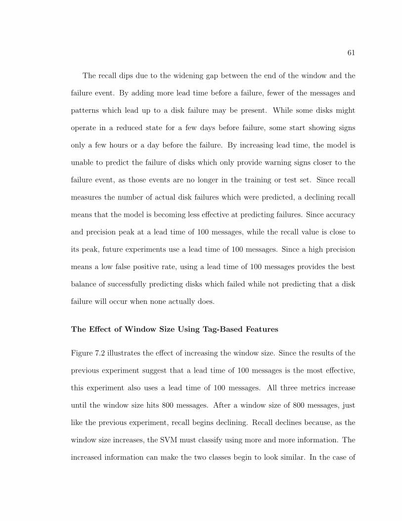
61

The recall dips due to the widening gap between the end of the window and the

failure event. By adding more lead time before a failure, fewer of the messages and

patterns which lead up to a disk failure may be present. While some disks might

operate in a reduced state for a few days before failure, some start showing signs

only a few hours or a day before the failure. By increasing lead time, the model is

unable to predict the failure of disks which only provide warning signs closer to the

failure event, as those events are no longer in the training or test set. Since recall

measures the number of actual disk failures which were predicted, a declining recall

means that the model is becoming less effective at predicting failures. Since accuracy

and precision peak at a lead time of 100 messages, while the recall value is close to

its peak, future experiments use a lead time of 100 messages. Since a high precision

means a low false positive rate, using a lead time of 100 messages provides the best

balance of successfully predicting disks which failed while not predicting that a disk

failure will occur when none actually does.

The Effect of Window Size Using Tag-Based Features

Figure 7.2 illustrates the effect of increasing the window size. Since the results of the

previous experiment suggest that a lead time of 100 messages is the most effective,

this experiment also uses a lead time of 100 messages. All three metrics increase

until the window size hits 800 messages. After a window size of 800 messages, just

like the previous experiment, recall begins declining. Recall declines because, as the

window size increases, the SVM must classify using more and more information. The

increased information can make the two classes begin to look similar. In the case of

62

200 300 400 500 600 700 800 900 1000 110050

55

60

65

70

75

80

85

90

95

100The Effect of Window Size On SVM Performance

Window Size

Per

cent

age

AccuracyPrecisionRecall

Figure 7.2: A graph of the effect of increasing window size (in messages)

disk failures, the disks only produce warning signs for a certain period of time. Before

these warning signs appear, they operate as normal disks. By adding information

from before the disks start to fail, that disk acts more like a working disk than a

failing disk. Since recall measures the effectiveness of the model at predicting disk

failures which actually failed, a low recall means the model is no longer predicting

disk failures as well. In addition, the false positive rate is lowest using 800 messages.

Future experiments will use a window size of 800 messages.

The Effect of Sequence Length on Predictions

The previous experiments all use sequences of length 5. This experiment varies the

sequence length between sequences of length 3 and sequences of length 8. While

increasing the sequence length may increase the effectiveness of the model, the increase

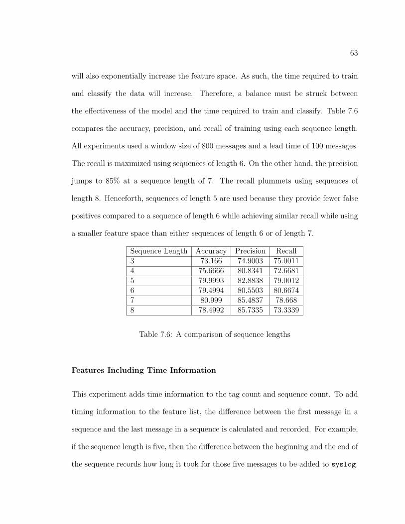
63

will also exponentially increase the feature space. As such, the time required to train

and classify the data will increase. Therefore, a balance must be struck between

the effectiveness of the model and the time required to train and classify. Table 7.6

compares the accuracy, precision, and recall of training using each sequence length.

All experiments used a window size of 800 messages and a lead time of 100 messages.

The recall is maximized using sequences of length 6. On the other hand, the precision

jumps to 85% at a sequence length of 7. The recall plummets using sequences of

length 8. Henceforth, sequences of length 5 are used because they provide fewer false

positives compared to a sequence of length 6 while achieving similar recall while using

a smaller feature space than either sequences of length 6 or of length 7.

Sequence Length Accuracy Precision Recall3 73.166 74.9003 75.00114 75.6666 80.8341 72.66815 79.9993 82.8838 79.00126 79.4994 80.5503 80.66747 80.999 85.4837 78.6688 78.4992 85.7335 73.3339

Table 7.6: A comparison of sequence lengths

Features Including Time Information

This experiment adds time information to the tag count and sequence count. To add

timing information to the feature list, the difference between the first message in a

sequence and the last message in a sequence is calculated and recorded. For example,

if the sequence length is five, then the difference between the beginning and the end of

the sequence records how long it took for those five messages to be added to syslog.

64

Therefore, the timing information provides a measure of message arrival rate. This

information is added to the feature space to discern whether a disk failure tends to

be accompanied by an increase or decrease in message rate. The number of times a

given time difference appears is recorded and added to the feature space.

The performance of classification using timing information is compared to the

performance without timing information in Table 7.7 and 7.8. In neither case did

the addition of time differentials significantly increase any of the three metrics. In

the case of length 5 sequences, the recall actually gets substantially worse. When

using sequences of length 7, the results with and without time are almost identical,

as seen in Table 7.8. In both cases, the recall may dip because the message logging

rate of nodes on a which a failure is going to occur within the next 100 messages is

similar to the message logging rate of nodes which are not predicted to fail. Since the

two rates are similar, the inclusion of timing information makes the two classes look

more similar than when no timing information is included. Therefore, the addition

of timing information not only does not provide improvement over tag sequences

without timing information, but it also increases the feature space. As a result, tag

based features are best when used without timing information.

Feature Space Accuracy Precision RecallSequences Using Tags 79.9993 82.8838 79.0012Sequences Using Tags and Time 77.8329 82.2338 71.667

Table 7.7: Comparing performance between features using only tags and featuresincluding time information using sequences of length 5

65

Feature Space Accuracy Precision RecallSequences Using Tags 80.999 85.4837 78.668Sequences Using Tags and Time 81.1661 86.9337 76.005

Table 7.8: Comparing performance between features using only tags and featuresincluding time information using sequences of length 7

7.3 Keystring Approaches

Chapter 2 states that there are many possible configurations for syslog data. The

one field that is almost certain to be in a configuration is the message field. Since

the message field is always present, whereas tag numbers might not be, this section

attempts to build a classifier using only information contained in the message field.

7.3.1 Preprocessing

As explained in Chapter 4, the input space created by using each unique string in the

syslog message field is too large to be able to calculate string sequences. Therefore,

a collection of dictionaries of useful strings is created. The dictionaries map strings

identified as important by SVM-Light to either 54, 24, or 23 unique values.

The preprocessing stage for keystring approaches is similar to the preprocessing

required by tag-based approaches. First, all of the strings in the message field are

replaced by the numerical value assigned to them by the current dictionary. If a string

is not in the dictionary, then it is removed from the file entirely. The time field and

the message field are isolated. A “+1” is appended to the end of messages which

contain a disk failure message. Conversely, a “-1” is appended to messages which do

not contain a failure message.

Next, each file is divided into a designated window size. If there are not enough

66

lines in a file before a disk failure to create the desired window, then that failure is

removed from the data set. Also, if a given disk fails within 24 hours of a previous

disk failure on that node, the latter failure is removed. Once the window is created,

then a number of messages are removed from the end of the file to simulate the desired

lead time.

Finally, a count of the number of times each keystring appears in a given file is

made. For each sequence of the specified length, a sequence number is calculated. A

count of these sequence numbers is kept and added to the data set. Once the data set

is created, an SVM is trained and tested using hold out and 10-fold cross validation.

7.3.2 Results Using Keystring Sequences Without Time In-

formation

The initial dictionary contains 54 keystrings. However, 25 of the strings in this dic-

tionary are the names of nodes on the cluster. To see whether or not the SVM is

learning what nodes tend to fail instead of actual patterns which lead to failures,

two other dictionaries are tested. One dictionary, made up of 24 keystrings, assigns

all keystrings of a given type to a single number. For example, all node names are

assigned a 0 and all number strings are assigned a 23. In the 24 keystring dictionary,

all node names, even those not in the original 54 keystring dictionary, are included.

Finally, a dictionary of 23 keystrings is tested in which all node names are removed.

The results of these three experiments using a window size of 800 messages, lead time

of 100 messages and sequences of length 3 are recorded in Table 7.9. The fact that

the 54 keystring and 24 keystring dictionaries perform similarly well suggests that

67

the SVM is not training on specific node names. Instead, the SVM is learning that

the appearance of any node name is useful for predicting failures. That the addition

of node names is useful for classification is clear when comparing the 24 keystring

dictionary to the 23 keystring dictionary. The 24 keystring dictionary has the ben-

efit of reducing the alphabet size dramatically when compared to the 54 keystring

dictionary, and thus a reduced feature space. As a result, all keystring experiments

henceforth use the 24 keystring dictionary.

Dictionary Accuracy Precision Recall54 77.6661 81.8171 76.000824 77.6659 79.1004 78.667623 73.8329 78.3172 72.668

Table 7.9: A comparison of keystring dictionaries

Table 7.11 shows the change in performance as the sequence length increases when

using the 24 keystring dictionary. Sequence of length 4 perform significantly better

across the board than those of length 3. While length 5 sequences perform slightly

better than those of length 4, the improvement is not significant with respect to recall,

although the false positive rate dips slightly. Since length 5 sequences significantly

increase the feature space with marginal benefit, the 24 keystring dictionary performs

best when using sequences of length 4.

Sequence Length Accuracy Precision Recall3 77.6659 79.1004 78.66764 79.4996 82.9838 80.66765 82.1428 85.0008 80.9543

Table 7.10: Performance as sequence length increases

68

7.3.3 Keystring Sequences Using Time

Adding time information to tag number sequences not only offers no improvement

over tag number sequences without temporal features, the addition of time informa-

tion actually results in the classifier performing worse. Despite the ineffectiveness

of combining timing information with tag sequences, the usefulness of timing with

regards to the keystring based approach is tested. If timing information is useful with

this approach, then it will have to be added to the final test, in which the feature space

combines both the tag and word based approaches. However, if timing information

does not help either method, then it can be left out of the final experiment.

Table 7.12 compares the performance of the 24 keystring approach both with and

without timing information. The sequence length used for both experiments is 4.

The accuracy and recall values of both approaches are essentially the same. However,

when using time information, there is a slightly lower false positive rate. Since a

lower false positive rate means fewer instances when a node goes into a preemptive

maintenance stage, minimizing the false positives is a worthy goal. While the feature

space increases, a system administrator may be willing to endure the longer training

and classification time if it results in fewer false positives. Thus, time information

keystring sequences are added to the final experiment.

Experiment Accuracy Precision RecallWithout Time Info 79.4996 82.9838 80.6676With Time Info 80.1657 85.567 78.6679

Table 7.11: A comparison of the 24 keystring dictionary with and without the additionof time information

69

7.4 Combination of Keystrings and Tag Sequences

Classifying works almost identically well when using tag number sequences of length 5

as when using keystring sequences of length 4. A comparison of the three measurement

metrics of both approaches is show in Table 7.12. The use of tag number sequences

achieves a slightly higher true positive rate while keeping a similar accuracy and

recall. If the tag-based approach and the keystring-based approach are learning on

different patterns, then perhaps combining the two approaches will result in better

classifications.

Approach Accuracy Precision RecallTag Sequences 80.999 85.4837 78.668Keystring Sequences 79.4996 82.9838 80.6676

Table 7.12: A comparison of tag-based and keystring-based methods

The process of combining features begins, as in all methods, by scanning through

files and retaining only the necessary data. In this case, the timestamp, tag number,

and numerical representation only of strings found in the keystring dictionary are

saved. Each line which signaled a disk failure is trailed by a +1 and a -1 is added to

lines which do not report a failure. Each file is broken up into a specified window size,

in this case 800 messages, and the desired lead time, 100 messages, is removed from

the end of the file. The window size and lead time were determined using the values

determined in past experiments. Tag sequences of length 5 are used, while keystring

sequences are 4 keystrings long. First, the number of appearances each tag number

makes in a given file is counted. Then, the tag number sequences are calculated and

counted. The appearances of each keystring and each keystring sequence are then

70

tallied. Since the addition of timing information hurt performance with tag based

features, timing information for sequences of length 5 is not calculated. However,

since the addition of temporal features is useful with keystring based features, time

differences are calculated for sequences of length 4.

Approach Accuracy Precision RecallTags Without Time 80.999 85.4837 78.668Keystrings With Time 80.1657 85.567 78.6679Combination Without Time 77.9995 82.317 74.334Combination With Time 80.6664 88.567 74.6673

Table 7.13: A comparison of tag based, keystring based, and combination methods

Table 7.13 provides a comparison among the best performing tag based approach,

the best keystring approach, and a combination approach both with and without

time information. Neither a combination of tag and keystring features with or without

additional timing information offers any substantial increase in accuracy and both see

a dip in recall, which means the combination model predicts fewer of the failures that

occur. The recall dips because the message rate does not provide a good indicator

of a failure. As a result, the inclusion of time information makes the two classes

look more similar. However, this increased similarity results in higher precision. The

precision increases because disks which were predicted to fail with low confidence

when omitting timing information are now predicted to continue working. Therefore,

only disks that have a high confidence score for failure are still predicted to fail. With

the combination of approaches and time information, the decrease in the number

of failures predicted is balanced by an increased true positive rate, meaning that

almost 89% of the disk failures predicted by this approach do fail within the next 30

71

hours. In fact, this model has the highest true positive rate of any of the experiments,

which means that the combination approach in conjunction with timing information

provides a useful improvement over other models. Whether or not it is the best model

depends on whether a higher recall rate or fewer false positives is the most desired

trait in a given situation.

Chapter 8: Conclusions and Future Work

Disk failures can result in significant data loss, especially in large computer clus-

ters. Every time a disk fails, jobs that are currently running must be restarted and the

data on the failed disk must be reconstructed. While the data can be recovered, the

reconstruction still takes time, during which the cluster is running below capacity. By

predicting failures before they happen, jobs can be scheduled so that no new jobs are

started on nodes which are about to have a disk failure. Also, the disk reconstruction

process can be started before the disk fails, which will minimize overall downtime.

The research presented in this thesis uses syslog event data to predict failures.

For each failure or non-failure event, a window of messages preceding the event is

taken. After each window, there is a set amount of lead time before the event being

predicted. For example, a given set up has a window of 500 messages with one day

between the final message in this window and the event being predicted. Features

are then extracted only from these windows. The features used are made up of a

combination of tag numbers, timestamps, and key words. Within each window, a

sliding window is used to create sequences of either tag numbers or key words. A

count of the number of times that each feature appeared is recorded. Finally, an

SVM is trained and then tested on the feature counts using hold out and ten fold

cross validation.

There are four goals of this research. The first goal is to develop a model which

could create useful predictions. Depending on the feature space used, one can attain

72

73

either a true positive rate of 85% while catching 79% of all disk failures or increase

the true positive rate to 88% while the number of disk failures predicted falls to 75%.

In either case, 75% of disk failures can be predicted before they happen using this

approach.

The second goal dictates that the information used to classify be commonly avail-

able so the approach can be deployed on the widest variety of systems. This research

utilized syslog event logs as data. Since syslog is installed by default on Linux and

Unix-based systems like Solaris, this data is widely available. Since this research is

specifically focused on the problem of disk failures in computer clusters, the use of

syslog is even more general than in the PC market, as many computer clusters run

Linux or Unix-based systems [30].

The third goal is to ensure that processing, training on, and classification of the

data is both simple and fast. Data processing is very simple. All one must do is isolate

the desired fields in the syslog file. After a basic translation step to transform the

syslog data into the alphabet for a given feature space, one must simply count

the number of times a given tag number of keystring appears in a file as well as

run each value through a single equation to gain sequence information. In addition,

training and classifying using a model of up to and including length 8 sequences for

tag numbers and length 4 for keystring sequences takes between a few seconds and

a few minutes; therefore both the training and classification steps can be performed

quickly.

The fourth goal is to provide a significant lead time in predictions. For example,

predicting a disk failure thirty seconds before it happens does not provide a system

74

administrator with enough time to start a maintenance cycle or fetch a replacement

disk drive. However, a lead time of a day allows the completion of both of these tasks.

The most accurate method studied used a lead time of 100 syslog messages. Since

there are an average of 78 syslog messages a day per node in the training set, a 100

message lead time equates to about 30 hours’ warning. As shown in Figure 7.1, it is

possible to increase the lead time to about 300 messages, or about 4 days, with only

slightly reduced accuracy, precision, and recall.

8.1 Comparison of Methods

The best method depends on three factors: the number of features one wishes to use

to classify on, the number of disk failures that can be predicted ahead of time, and

the true positive rate. While it is important to predict disk failures, the usefulness

of the model diminishes if, for example, it predicts all disk failures, but also predicts

three times the number of failures that actually occur. In this case, many disks which

did not fail will be replaced, which both requires the money to buy replacement disks

and wastes the disks which are already installed. In addition, the time a system

administrator spends replacing disks which do not fail could have been used on other

tasks.

To determine the overall best method, this section considers the true positive rate

as well as the recall. In addition, this section proposes an event logging system which

requires less storage space than the current syslog utility.

75

8.1.1 Balance Between True Positives and Failures Predicted

As explained above, both a high true positive rate and high recall are important when

classifying failures. However, which is more important depends on the goal of a given

company or administrator. Some might be willing to trade off misclassifying a few

disks as failures as long as more actual failures are caught. Thus, if a high recall is

the more important goal, the best approach is to use either tag sequences without

timing information or keystring sequences using the 24 keystring dictionary with

timing information. Both approaches hit almost 80% recall. In addition, both had

very few misclassified failures. As explained below, the space requirements using only

tag sequences or keystring sequences are almost identical, although the tag sequences

can save more space if one is willing to remove the unneeded timestamp. Section 8.2

will also discuss why the use of keywords plus time information is preferable to an

approach using only tag numbers. If a high true positive rate is the most desired

classification trait for a given situation, then there is only one choice: combining tag

sequences with keystring sequences and timing information, as this approach has a

true positive rate of 89% while still predicting 75% of disk failures.

8.1.2 Space Requirements

Space Required By Full Syslog

First, consider the space required by retaining all fields of the syslog system. As

clusters grow in size, more and more machines are recording syslog info. As a result,

the amount of storage space needed to keep all of these syslog records is also increas-

ing. Consider the PNNL data set used for this experiment. On average, there were 78

76

syslog messages an hour for each node. As a result, there were approximately 1,872

messages per day. Since there were 1024 nodes, there are approximately 1,916,928

total messages per day and 699,678,720 messages on the cluster every year.

Now that the number of messages per year is known, it is important to figure out

how much space on average a syslog message requires. Each character in a syslog

file is 1 byte. The host field requires eight bytes. Similarly, the facility field uses

about four bytes on average, as does the level. The tag field requires three bytes and

the time requires ten bytes. The number of the characters in the message field can

vary greatly, but assume that an average message consists of five words, which is a

low-end estimate. Then assume that each word uses about five characters. Between

each field there is one space, which also requires one byte. As a result, the average

syslog message uses up 64 bytes. One year of syslog data for this system therefore

requires 41.7 GB.

Now consider that using only keywords or tag numbers to predict failures is rather

effective. If one can predict events using only tag numbers or keywords, then perhaps

one could keep only the fields required for these predictions. At the very least, since

each node keeps a copy of its syslog and the central server has a record of every

node’s syslog events, perhaps the space requirement can be reduced on at least one

of the two machines by storing only a subset of the required fields.

Space Required By Tag Based Approaches

First, consider the approach using tag numbers. It is easier to justify getting rid of

most of the fields using tag numbers than it is when using keywords. First, to ensure

77

that the node number is not lost, the syslog facility could keep each node’s record in

a separate file. The level field is also easy to justify getting rid of, as the tag number

provides a more fine-grained indication of a message’s importance. Since the tag

number approach itself removes keywords under the assumption that the tag number

is specific enough to indicate how important a message is, both both the facility and

message fields are removed. Notice that this approach removes the entire message

field, meaning that a system administrator is unable to look at the logs later to glean

any meaningful information as to what has happened on a given system. This analysis

is considering a situation where the only value in the log file is the ability to predict

events.

At this point, the proposed syslog configuration uses only the ten byte time field

and a three byte tag field as well as a one byte space between the two fields. As a

result, each message requires fourteen bytes. Therefore, 9.122 GB per year is required

to keep every message from every node on the cluster. The altered syslog setup uses

21.875% as much space as a configuration which includes all six fields. However, if

one removes the timestamps from each message and retains only the tag information,

one can reduce the space needed to 1.95 GB per year. This is a massive reduction and

makes the tag sequence approach ideal if saving space is a concern. Remember that

absolutely no semantic information or temporal information of any kind is retained in

this case, so one must be absolutely sure that the log files will only be used for failure

prediction and nothing else. A situation of this sort is unlikely in the real world, but

is presented here for completeness.

78

Space Required by Keystring Based Approaches

The tag based approach to saving space detailed in the previous section eliminates all

semantic information, which is not realistic. However, retaining only the keystrings

does retain some semantic information. An analysis of the number of keywords present

in each message in the data set revealed that each message contains an average of 0.59

keywords. Since each keyword is assumed to be 5 characters long, that comes out to

2.95 characters per message. Each message thus takes up 13.95 bytes per message for

a total of 9.09 GB per year. Therefore, the words and time approach uses 21.7883%

of space that a full syslog entry does. However, as with tag-based approaches, a

human is unlikely to be able to look at a log file which contains only keystrings and

timestamps and glean any useful knowledge. Therefore, the next section examines

the space one can save by keeping only the timestamp and the entire message field.

Space Required When Keeping All Messages

While the approach which marries tag numbers and timing information is the best

combination of speed and accuracy, combining the keywords with timing information

performs the best overall. Keeping keywords provides another benefit over just keep-

ing tags: some amount of semantic data is retained. Keeping some form of semantic

data would be useful should a system administrator need to look at and make sense of

the logs. It is a legitimate question as to whether or not keeping only a keyword here

or there would even be useful. For the sake of argument, assume all words are kept.

Keeping all of the words allows the same data to be broken up using a different set

of keywords if a user is trying to predict another type of event or if a more effective

79

keyword list for the current problem is found. In this case, the only fields that are

necessary are the timing information and the message itself, as the level, facility, and

tag numbers add nothing to this prediction approach. As a result, each message will

be 31 bytes on average, which will take up 20.2 GB per year for a 51.563% reduction

on the overall storage space needed.

8.1.3 The Best Method

Since, in a real world setting, one would need to keep all of the messages for future

examination by humans, the keystring based approach with time is the best approach

if the main goal is a high recall. One can save more space by removing the tag

numbers. Since the tag based and keystring-with-time approaches both perform the

same, there is no performance lost by removing tag numbers. Removing unnecessary

fields still eliminates over 50% of the total space required by syslog. Semantic

information is retained for use by human readers and this information can be parsed

for the necessary keystrings when performing predictions.

Maximizing precision requires that one keep the tag numbers as well. Keeping

tag numbers as well as timestamps and the message field uses 22.8 GB per year.

Therefore, one would need to keep about 2.6 more GB per year than when using only

keystrings to maximize recall. However, this still represents a marked improvement

over the space required by standard syslog and is the best choice if one wishes to

minimize the false positive rate.

80

8.2 Future Work

There are two branches this research can take immediately. The first direction is to

try different classification methods. This thesis only examines the effectiveness of

the SVM approach to classifying nodes as likely to fail. However, other classification

methods exist. Other supervised learning approaches, such as the nearest neighbor

algorithm, are one possibility. In addition, perhaps unsupervised learning methods

would prove fruitful.

Another direction this research could move in is to try to predict other events.

The approach discussed in this thesis only examines the usefulness of using various

features with an SVM to predict disk failures. Perhaps this same approach could

be used to predict whether or not an entire node is going to go offline or if a RAID

controller is going to fail. One would simply need to find these events in the logs and

label each feature vector appropriately before training. Otherwise, the approach, as

far as finding sequence numbers or keywords, is exactly the same.

The generalizability of this approach should also be examined by applying the ap-

proach to different data sets. The goal of this research is not to create one model which

will work for all syslog or cluster configurations. Instead, this research presents an

approach which can be used to build a model for a given cluster. For example, a clus-

ter may have a different syslog configuration, average message rate, or applications

which are installed than those seen in the data set used for this thesis. Rather than

using the exact model generated on the data set used in this thesis on this second

cluster, one should use the approach detailed in this thesis to create a model for the

second cluster. However, other data sets must be used to see whether or not this

81

approach is useful on cluster configurations other than the one in the data set used

for this thesis.

82

54 Keystring Dictionary

The 54 keystrings used for predicting disk failures. Every occurrence of each

keystring in a given syslog file was replaced with the corresponding number. These

numbers were then used for the creation of keystring sequences.

Keystring Assigned Number

m800 0m758 1m851 2m28 3configuration 4scsi 5hpc7 6m382 7rev 8m301 9sdd5 10m126 11m162 120105 13shutdown 14using 15sdd4 16reset 17m317 1814832384 19usb 20rx2600 21m339 22m789 2314 24kernel 25status 26session 27user 28times 29m579 30root 31zx6000 32m225 33command 346143936 35m309 36m926 37m212 38pci 39for 408 41this 42lustre 43m876 44m508 45m65 46hpc5 47m287 48m11 49m525 50m377 51m48 52m104 53

References

[1] Bruce Allen. Monitoring hard disks with smart. Linux Journal, 1(117), January2004. Available at: http://www.linuxjournal.com/magazine/monitoring-hard-disks-smart. Accessed on April 19, 2010.

[2] David A. Bader and Robert Pennington. Cluster computing: Applications.The International Journal of High Performance Computing, 15(2):181–185, May2001.

[3] Gokhan H. Bakir, Leon Bottou, and Jason Weston. Breaking svm complexitywith cross-training. In Advances in Neural Information Processing Systems 17.The MIT Press, 2005.

[4] B.E. Boser, I. Guyon, and V.N. Vapnik. A training algorithm for optimal mar-gin classifiers. In Proceedings of the Fifth Annual Workshop of ComputationalLearning Theory 5, pages 144–152, 1992.

[5] Peter Broadwell. Component failure prediction using super-vised naive bayesian classification, December 2002. Available at:http://citeseerx.ist.psu.edu/viewdoc/summary?doi=10.1.1.3.4641. Accessedon April 19, 2010.

[6] Christopher J.C. Burges. A tutorial on support vector machines for patternrecognition. Data Mining and Knowledge Discovery, 2:121–167, 1998.

[7] Olivier Chapelle, Bernhard Scholkopf, and Alexander Zien. Semi-SupervisedLearning. The MIT Press, 2006.

[8] Corinna Cortes and Vladimir Vapnik. Support-vector networks. Machine Learn-ing, 20:273–297, 1995.

[9] Peter Dayan. Unsupervised learning. In Robert A. Wilson and Frank Keil,editors, The MIT Encyclopedia of the Cognitive Sciences. The MIT Press, 1999.

[10] Thomas G. Dietterich. Machine learning for sequential data: A review. InProceedings of the Joint IAPR International Workshop on Structural, Syntactic,and Statistical Pattern Recognition, pages 15–30. Springer-Verlag, 2002.

[11] Rober P.W. Duin and Elzbieta Pekalska. The science of pattern recognition,achievements and perspectives. Studies in Computational Intelligence, 63:221–259, 2007.

83

84

[12] Ronald A. Fischer. The use of multiple measurements in taxonomic problems.Annals Eugen, 7:179–188, 1936.

[13] Errin W. Fulp, Glenn A. Fink, and Jereme N. Haack. Predicting computersystem failures using support vector machines. In First USENIX Workshop onthe Analysis of Logs (WASL), 2008.

[14] Z. Ghahramani. Unsupervised learning. In Advanced Lectures on MachingLearning LNAI 3176. Springer-Verlag, 2004.

[15] Greg Hamerly and Charles Elkan. Bayesian approaches to failure predictionfor disk drives. In Proceedings of the Eighteenth International Conference onMachine Learning (ICLM), June 2001.

[16] Thorsten Joachims. Making Large-Scale SVM Learning Practical. The MITPress, 1999.

[17] Thorsten Joachims. Training linear svms in linear time. In Proceedings of theACM Conference of Knowledge Discovery and Data Mining (KDD). ACM, 2006.

[18] Andrew Karode. Support vector machine classification of network streams usinga spectrum kernel encoding. Master’s thesis, Wake Forest University, December2008.

[19] Christina Leslie, Eleazar Eskin, and William Stafford Noble. The spectrumkernel: A string kernel for svm protein classification. In Proceedings of the PacificSymposium on Biocomputing 7, January 2002.

[20] Yinglung Liang, Yanyong Zhang, Hui Xiong, and Ramendra Sahoo. Failureprediction in ibm bluegene/l event logs. In Proceedings of the Sevent IEEEInternational Conference on Data Mining, 2007.

[21] C. Lonvick. The bsd syslog protocol, 2001. Available at:http://www.faqs.org/rfcs/rfc3164.html. Accessed on: April 19, 2010.

[22] John Makhoul, Francis Kubala, Richard Schwartz, and Ralph Weischedel. Per-formance measures for information extraction. In Proceedings of DARPA Broad-cast News Workshop, pages 249–252, 1999.

[23] Joseph F. Murray, Gordon F. Hughes, and Kenneth Kreutz-Delgado. Hard drivefailure prediction using non-parametric statistical methods. In Proceedings ofICANN/ICONIP, June 2003.

[24] E. Pinheiro, W.D. Webe, and L.A. Barroso. Failure trends in a large disk drivepopulation. In Proceedings of the 5th USENIX Symposium on File and StorageTechnologies (FAST ’07), February 2007.

85

[25] R.K. Sahoo, A.J. Oliner, I. Rish, M. Gupta, J.E. Moreira, and S. Ma. Criticalevent prediction for proactive management in large-scale computer clusters. InProceedings of the Ninth ACM SIGKDD International Conference of KnowledgeDiscovery and Data Mining, August 2003.

[26] Minoru Sasaki and Kenji Kita. Rule-based text categorization using hierarchicalcategories. In Proceedings of the IEEE International, pages 2827–2830, 1998.

[27] Bianca Schroeder and Garth A Gibson. Understanding failures in petascalecomputers. Journal of Physics: Conference Series, 28, 2007.

[28] Abraham Silberschatz, Henry F. Korth, and S. Sudarshan. Database SystemsConcepts. McGraw Hill, 5th edition, 2006.

[29] John Simpson and Edmund Weiner, editors. Oxford English Dictionary, vol-ume 1. Oxford University Press, second edition, 1989.

[30] Top500. Operating system share for 11/2009. Available at:http://www.top500.org/stats/list/34/osfam. Accessed on April 19, 2010.

[31] Ivor W. Tsang, James T. Kwok, and Pak-Ming Cheung. Core vector machines:Fast svm training on very large data sets. Journal of Machine Learning Research,6, 2005.

[32] William H. Turkett, Andrew V. Karode, and Errin W. Fulp. In-the-dark networktraffic classification using support vector machines. In Proceedings of the AAAIConference on Artificial Intelligence, 2008.

[33] Doug Turnbull and Neil Alldrin. Failure prediction in hardware systems, 2003.Available at: http://www.cs.ucsd.edu/ dturnbul/Papers/ServerPrediction.pdf.Accessed on: April 19, 2010.

[34] Ian H. Witten and Eibe Frank. Data Mining: Practical Machine Learning Toolsand Techniques. Morgan Kauffman, second edition, 2005.