Design of low-propped embedded retaining walls in stiff clays
Proceedings of the Institution of Civil Engineers
Geotechnical Engineering 166 October 2013 Issue GE5
Pages 466–482 http://dx.doi.org/10.1680/geng.11.00079
Paper 1100079
Received 27/08/2011 Accepted 16/04/2012
Published online 03/09/2012
Keywords: excavation/mathematical modelling/tunnels & tunnelling
ICE Publishing: All rights reserved
Geotechnical EngineeringVolume 166 Issue GE5
Predicting ground movements in LondonClayJurecic, Zdravkovic and Jovicic
Predicting ground movementsin London Clayj1 Nina Jurecic
Research Assistant, Institute of Mining, Geotechnology andEnvironment (IRGO), Ljubljana, Slovenia
j2 Lidija Zdravkovic MEng, MSc, PhD, DICReader in Computational Soil Mechanics, Imperial College London,London, UK
j3 Vojkan Jovicic MEng, MSc, PhDLecturer in Geotechnics, Institute of Mining, Geotechnology andEnvironment (IRGO), Ljubljana, Slovenia
j1 j2 j3
The necessity of accounting for small-strain behaviour of soils in numerical analyses of the serviceability limit states
of geotechnical structures is well established both nationally and internationally. This has led to further development
of appropriate soil constitutive models, as well as to further advances in accurate laboratory measurements of small-
strain stiffness. The current paper considers recent laboratory research into the behaviour of London Clay, performed
at Imperial College in conjunction with the major ground works for Heathrow Terminal 5 in London, UK. This research
has shown the small-strain response of London Clay to be different to that assumed previously and in particular to
that determined from good-quality commercial experiments. Both sets of small-strain stiffness data are applied in
this paper in finite-element analyses of a deep excavation and a tunnel construction in London Clay, with the
objective of investigating their effect on predicted ground movements.
1. IntroductionAdvanced laboratory testing of geotechnical materials has en-
hanced our understanding of many aspects of soil behaviour.
Perhaps the most influential in recent years has been the
recognition of soil’s small-strain behaviour, which is charac-
terised, among other features, by non-linearity of soil stiffness at
small strains. A number of numerical studies of geotechnical
problems (e.g. finite-element or finite-difference analyses) have
shown that accounting for soil’s non-linear stiffness improves the
predictions of ground movements at serviceability limit states
(e.g. Addenbrooke et al., 1997; Higgins et al., 1996; Hight and
Higgins, 1994; Simpson et al., 1996; Stallebrass et al., 1994).
The constitutive modelling of small-strain behaviour of geotech-
nical materials has also evolved over the years, from simple non-
linear elastic empirical models (e.g. Jardine et al., 1986; Simpson
et al., 1979), to more advanced kinematic and bounding surface
models that can reproduce, in addition to non-linearity and
plasticity at early stages of loading, other advanced aspects of real
soil behaviour (Baudet and Stallebrass, 2004; Grammatikopoulou
et al., 2006; Kavvadas and Amorosi, 2000; Manzari and Dafalias,
1997).
Recent laboratory-based research on the behaviour of London
Clay, conducted at Imperial College and published largely in the
Geotechnique ‘Symposium in Print’ 2007 (vol. 51, issue 1), was
focused in part on the investigation of stiffness of natural London
Clay (Gasparre et al., 2007; Hight et al., 2007). In particular,
Hight et al. (2007) compared the stiffness decay curves of
London Clay, from samples taken at various depths and in various
lithological units, derived from earlier high-quality commercial
laboratory testing and from this recent research, and showed that
the two sets of results differ not only in the stiffness magnitude,
but also in their decay in the small-strain range.
Considering that significant experience and confidence has been
gained over the years in using the commercially derived stiffness
decay curves in predictions of ground movements in London Clay
(e.g. Higgins et al., 1996; Kanapathipillai, 1996; Schroeder et al.,
2011; Simpson, 1992), the availability of the new, and signifi-
cantly different, stiffness data for which there is no prior
experience in predicting ground movements, raises the question
as to which set of experimental evidence should be used in
representing the stiffness of London Clay in future numerical
analyses of geotechnical problems.
Hight et al. (2007) go some way to explain the reasons for the
differences in the two sets of stiffnesses, but recognise that this
needs further investigation. They also postulated that factors
related to stiffness anisotropy may help to explain this anomaly,
466Downloaded by [ Imperial College London Library] on [12/05/16]. Copyright © ICE Publishing, all rights reserved.
considering that the commercial stiffness decay curves provided
only isotropic stiffness, whereas Gasparre et al. (2007) contrib-
uted to further understanding of the small-strain stiffness
anisotropy of London Clay. A subsequent study of Grammatiko-
poulou et al. (2008), on a shallow propped excavation in London
Clay, indicated that there may be significant difference in
predicted wall and ground movements around such an excavation
when different sets of isotropic stiffness curves are used in
analyses.
Based on the above, the objective of the current paper is to
demonstrate the effects: (a) of the previous and the new isotropic
small-strain stiffness data, and (b) of using anisotropic as
opposed to isotropic small-strain stiffness data of London Clay
on predictions of ground movements. Two boundary value
problems are utilised for this purpose. The first one is the
excavation of the Jubilee Line extension tunnels at St James’s
park, for which there are measurements of ground movements
due to tunnel excavations that can be compared to numerical
predictions (i.e. class C analyses according to Lambe (1973)).
The second example is a deep excavation at Moorgate, on the
Crossrail route, which has not yet been constructed and hence the
numerical predictions are before the event (i.e. class A analyses).
It is further emphasised that in each of the two studies all other
numerical details (e.g. initial stresses, permeability, constitutive
models and boundary conditions) are the same, only the small-
strain stiffness of London Clay is varied. Also, the initial stresses
in the ground in each of the two studies correspond to
equilibrium greenfield conditions when the depositional history
of all the layers is completed. In terms of the non-linear small-
strain behaviour this means that the stiffness in the soil starts
from a respective elastic plateau and then degrades with the
increase in strain level due to the construction of tunnels or deep
excavation respectively. All analyses have been performed using
the finite-element software ICFEP (Potts and Zdravkovic, 1999),
which employs the modified Newton–Raphson method with an
error-controlled sub-stepping stress-point algorithm as its non-
linear solver.
2. Calibration of constitutive modelsConsidering the objectives of this study, the main emphasis in
the calibration process has been on the small-strain stiffness of
London Clay, adopting the same modelling framework for both
the old and the new stiffness data. The chosen constitutive
model is a form of a non-linear elastic and non-associated
plastic Mohr–Coulomb model (Potts and Zdravkovic, 1999).
The non-linearity below the Mohr–Coulomb yield surface
accounts for stiffness variation with both stress and strain
levels. The isotropic non-linear model allows independent input
of the shear and the bulk stiffness parameters, according to the
Jardine et al. (1986) non-linear expression given in the
Appendix. The anisotropic stiffness model, developed by Fran-
zius et al. (2005), adopts similar expressions for non-linear
stiffness variation (see Appendix), but the bulk stiffness is not
an independent input.
2.1 Available stiffness data
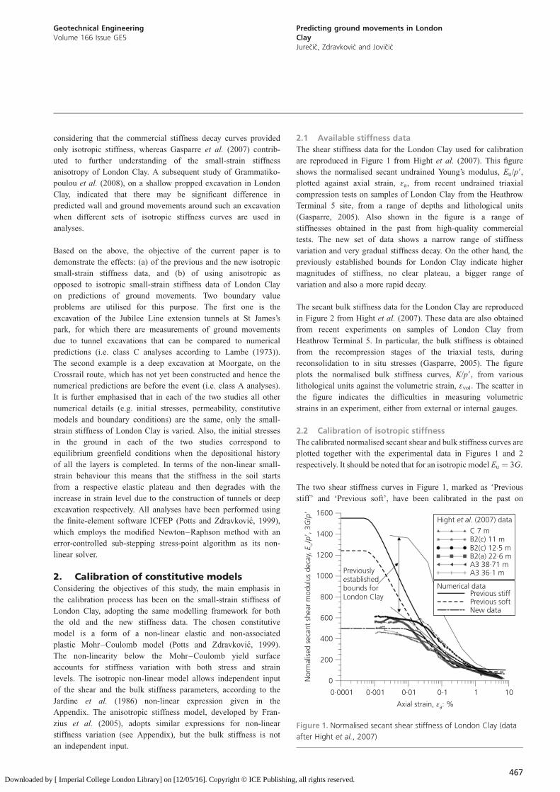
The shear stiffness data for the London Clay used for calibration
are reproduced in Figure 1 from Hight et al. (2007). This figure
shows the normalised secant undrained Young’s modulus, Eu/p9,
plotted against axial strain, �a, from recent undrained triaxial
compression tests on samples of London Clay from the Heathrow
Terminal 5 site, from a range of depths and lithological units
(Gasparre, 2005). Also shown in the figure is a range of
stiffnesses obtained in the past from high-quality commercial
tests. The new set of data shows a narrow range of stiffness
variation and very gradual stiffness decay. On the other hand, the
previously established bounds for London Clay indicate higher
magnitudes of stiffness, no clear plateau, a bigger range of
variation and also a more rapid decay.
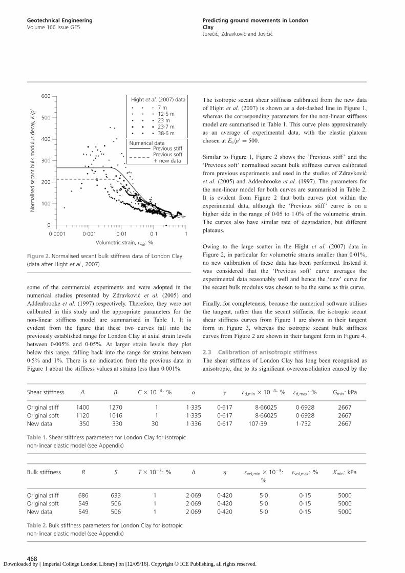
The secant bulk stiffness data for the London Clay are reproduced
in Figure 2 from Hight et al. (2007). These data are also obtained
from recent experiments on samples of London Clay from
Heathrow Terminal 5. In particular, the bulk stiffness is obtained
from the recompression stages of the triaxial tests, during
reconsolidation to in situ stresses (Gasparre, 2005). The figure
plots the normalised bulk stiffness curves, K/p9, from various
lithological units against the volumetric strain, �vol: The scatter in
the figure indicates the difficulties in measuring volumetric
strains in an experiment, either from external or internal gauges.
2.2 Calibration of isotropic stiffness
The calibrated normalised secant shear and bulk stiffness curves are
plotted together with the experimental data in Figures 1 and 2
respectively. It should be noted that for an isotropic model Eu ¼ 3G.
The two shear stiffness curves in Figure 1, marked as ‘Previous
stiff’ and ‘Previous soft’, have been calibrated in the past on
0
200
400
600
800
1000
1200
1400
1600
0·0001 0·001 0·01 0·1 1 10
Nor
mal
ised
sec
ant
shea
r m
odul
us d
ecay
,/
, 3/
Ep
G p
u�
�
Axial strain, : %εa
Previouslyestablishedbounds forLondon Clay
Hight . (2007) dataet alC 7 mB2(c) 11 mB2(c) 12·5 mB2(a) 22·6 mA3 38·71 mA3 36·1 m
Numerical dataPrevious stiffPrevious softNew data
Figure 1. Normalised secant shear stiffness of London Clay (data
after Hight et al., 2007)
467
Geotechnical EngineeringVolume 166 Issue GE5
Predicting ground movements in LondonClayJurecic, Zdravkovic and Jovicic
Downloaded by [ Imperial College London Library] on [12/05/16]. Copyright © ICE Publishing, all rights reserved.
some of the commercial experiments and were adopted in the
numerical studies presented by Zdravkovic et al. (2005) and
Addenbrooke et al. (1997) respectively. Therefore, they were not
calibrated in this study and the appropriate parameters for the
non-linear stiffness model are summarised in Table 1. It is
evident from the figure that these two curves fall into the
previously established range for London Clay at axial strain levels
between 0.005% and 0.05%. At larger strain levels they plot
below this range, falling back into the range for strains between
0.5% and 1%. There is no indication from the previous data in
Figure 1 about the stiffness values at strains less than 0.001%.
The isotropic secant shear stiffness calibrated from the new data
of Hight et al. (2007) is shown as a dot-dashed line in Figure 1,
whereas the corresponding parameters for the non-linear stiffness
model are summarised in Table 1. This curve plots approximately
as an average of experimental data, with the elastic plateau
chosen at Eu/p9 ¼ 500.
Similar to Figure 1, Figure 2 shows the ‘Previous stiff’ and the
‘Previous soft’ normalised secant bulk stiffness curves calibrated
from previous experiments and used in the studies of Zdravkovic
et al. (2005) and Addenbrooke et al. (1997). The parameters for
the non-linear model for both curves are summarised in Table 2.
It is evident from Figure 2 that both curves plot within the
experimental data, although the ‘Previous stiff’ curve is on a
higher side in the range of 0.05 to 1.0% of the volumetric strain.
The curves also have similar rate of degradation, but different
plateaus.
Owing to the large scatter in the Hight et al. (2007) data in
Figure 2, in particular for volumetric strains smaller than 0.01%,
no new calibration of these data has been performed. Instead it
was considered that the ‘Previous soft’ curve averages the
experimental data reasonably well and hence the ‘new’ curve for
the secant bulk modulus was chosen to be the same as this curve.
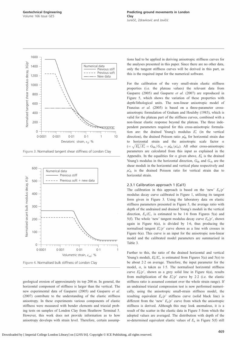
Finally, for completeness, because the numerical software utilises
the tangent, rather than the secant stiffness, the isotropic secant
shear stiffness curves from Figure 1 are shown in their tangent
form in Figure 3, whereas the isotropic secant bulk stiffness
curves from Figure 2 are shown in their tangent form in Figure 4.
2.3 Calibration of anisotropic stiffness
The shear stiffness of London Clay has long been recognised as
anisotropic, due to its significant overconsolidation caused by the
0
100
200
300
400
500
600
0·0001 0·001 0·01 0·1 1
Nor
mal
ised
sec
ant
bulk
mod
ulus
dec
ay,
/K
p�
Volumetric strain, : %εvol
Hight . (2007) dataet al
7 m12·5 m23 m23·7 m38·6 m
Numerical dataPrevious stiffPrevious soft
n� ew data
Figure 2. Normalised secant bulk stiffness data of London Clay
(data after Hight et al., 2007)
Shear stiffness A B C 3 10�4: % Æ ª �d,min 3 10�4: % �d,max: % Gmin: kPa
Original stiff 1400 1270 1 1.335 0.617 8.66025 0.6928 2667
Original soft 1120 1016 1 1.335 0.617 8.66025 0.6928 2667
New data 350 330 30 1.336 0.617 107.39 1.732 2667
Table 1. Shear stiffness parameters for London Clay for isotropic
non-linear elastic model (see Appendix)
Bulk stiffness R S T 3 10�3: % � � �vol,min 3 10�3:
%
�vol,max: % Kmin: kPa
Original stiff 686 633 1 2.069 0.420 5.0 0.15 5000
Original soft 549 506 1 2.069 0.420 5.0 0.15 5000
New data 549 506 1 2.069 0.420 5.0 0.15 5000
Table 2. Bulk stiffness parameters for London Clay for isotropic
non-linear elastic model (see Appendix)
468
Geotechnical EngineeringVolume 166 Issue GE5
Predicting ground movements in LondonClayJurecic, Zdravkovic and Jovicic
Downloaded by [ Imperial College London Library] on [12/05/16]. Copyright © ICE Publishing, all rights reserved.
geological erosion of approximately its top 200 m. In general, the
horizontal component of stiffness is larger than the vertical. The
new experimental data of Gasparre (2005) and Gasparre et al.
(2007) contribute to the understanding of the elastic stiffness
anisotropy. In these experiments various components of elastic
stiffness were measured with bender elements and triaxial prob-
ing tests on samples of London Clay from Heathrow Terminal 5.
However, this work does not provide information as to how
anisotropy develops with strain level. Therefore, certain assump-
tions had to be applied in deriving anisotropic stiffness curves for
the analyses presented in this paper. Since there are no other data,
only the tangent stiffness curves will be derived in this part, as
this is the required input for the numerical software.
For the calibration of the very small-strain elastic stiffness
properties (i.e. the plateau values) the relevant data from
Gasparre (2005) and Gasparre et al. (2007) are reproduced in
Figure 5, which shows the variation of these properties with
depth/lithological units. The non-linear anisotropic model of
Franzius et al. (2005) is based on a three-parameter cross-
anisotropic formulation of Graham and Houlsby (1983), which is
valid for the plateau part of the stiffness curves, combined with a
non-linear elastic response beyond the plateau. The three inde-
pendent parameters required for this cross-anisotropic formula-
tion are: the drained Young’s modulus E9v (in the vertical
direction), the drained Poisson ratio �9hh for horizontal strain due
to horizontal strain and the anisotropic scale factor Æ(¼
ffiffiffiffiffiffiffiffiffiffiffiffiffiE9h=E9v
p¼ Ghh=Gvh ¼ �9hh=�9vh). All other cross-anisotropic
parameters are calculated from this input as explained in the
Appendix. In the equalities for Æ given above, E9h is the drained
Young’s modulus in the horizontal direction, Ghh and Gvh are the
shear moduli in the horizontal and vertical plane respectively and
�9vh is the drained Poisson ratio for vertical strain due to
horizontal strain.
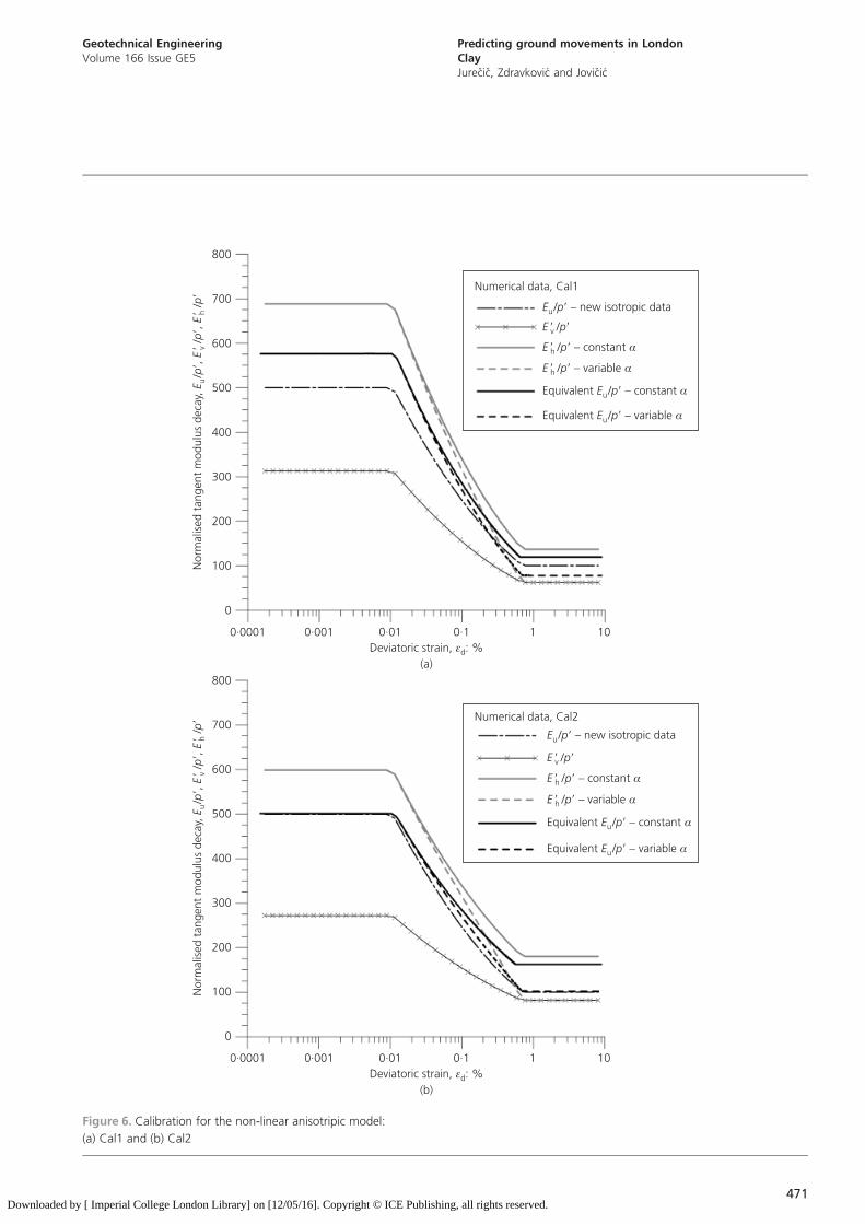
2.3.1 Calibration approach 1 (Cal1)
The calibration in this approach is based on the ‘new’ Eu/p9
modulus decay curve calibrated in Figure 1, utilising its tangent
form given in Figure 3. Using the laboratory data on elastic
stiffness parameters presented in Figure 5, the average ratio with
depth of the undrained and drained Young’s moduli in the vertical
direction, Eu/E9v, is estimated to be 1.6 from Figures 5(a) and
5(f). The whole ‘new’ tangent modulus decay curve Eu/p9, shown
again in Figure 6(a), is divided by 1.6, thus producing the
normalised tangent E9v/p9 curve shown as a line with crosses in
Figure 6(a). This curve is an input for the anisotropic non-linear
model and the calibrated model parameters are summarised in
Table 3.
Further to this, the ratio of the drained horizontal and vertical
Young’s moduli, E9h/E9v, is estimated from Figures 5(a) and 5(e) to
be about 2.2 on average. Therefore, the input parameter for the
model, Æ, is taken as 1.5. The normalised horizontal stiffness
curve E9h/p9, shown as a grey solid line in Figure 6(a), results
from multiplication of the E9v/p9 curve by 2.2 (i.e. the elastic
stiffness ratio is assumed constant over the whole strain range). If
an undrained triaxial compression test is now performed numeri-
cally, using the anisotropic small-strain stiffness model, the
resulting equivalent Eu/p9 stiffness curve (solid black line) is
different from the ‘new’ Eu/p9 curve from which the anisotropic
stiffness is derived. Although this may look anomalous, it is a
result of the scatter in the elastic data in Figure 5 from which the
adopted values are averaged. The distribution with depth of the
so-determined equivalent elastic values of Eu in Figure 5(f) still
0
200
400
600
800
1000
1200
1400
1600
0·0001 0·001 0·01 0·1 1 10
Nor
mal
ised
tan
gent
she
ar m
odul
us d
ecay
, 3/
G p
�
Deviatoric strain, : %εd
Numerical dataPrevious stiffPrevious softNew data
Figure 3. Normalised tangent shear stiffness of London Clay
0
100
200
300
400
500
600
0·0001 0·001 0·01 0·1 1
Nor
mal
ised
sec
ant
bulk
mod
ulus
dec
ay,
/K
p�
Volumetric strain, : %εvol
Numerical dataPrevious stiff
Previous soft n� ew data
Figure 4. Normalised bulk stiffness of London Clay
469
Geotechnical EngineeringVolume 166 Issue GE5
Predicting ground movements in LondonClayJurecic, Zdravkovic and Jovicic
Downloaded by [ Imperial College London Library] on [12/05/16]. Copyright © ICE Publishing, all rights reserved.
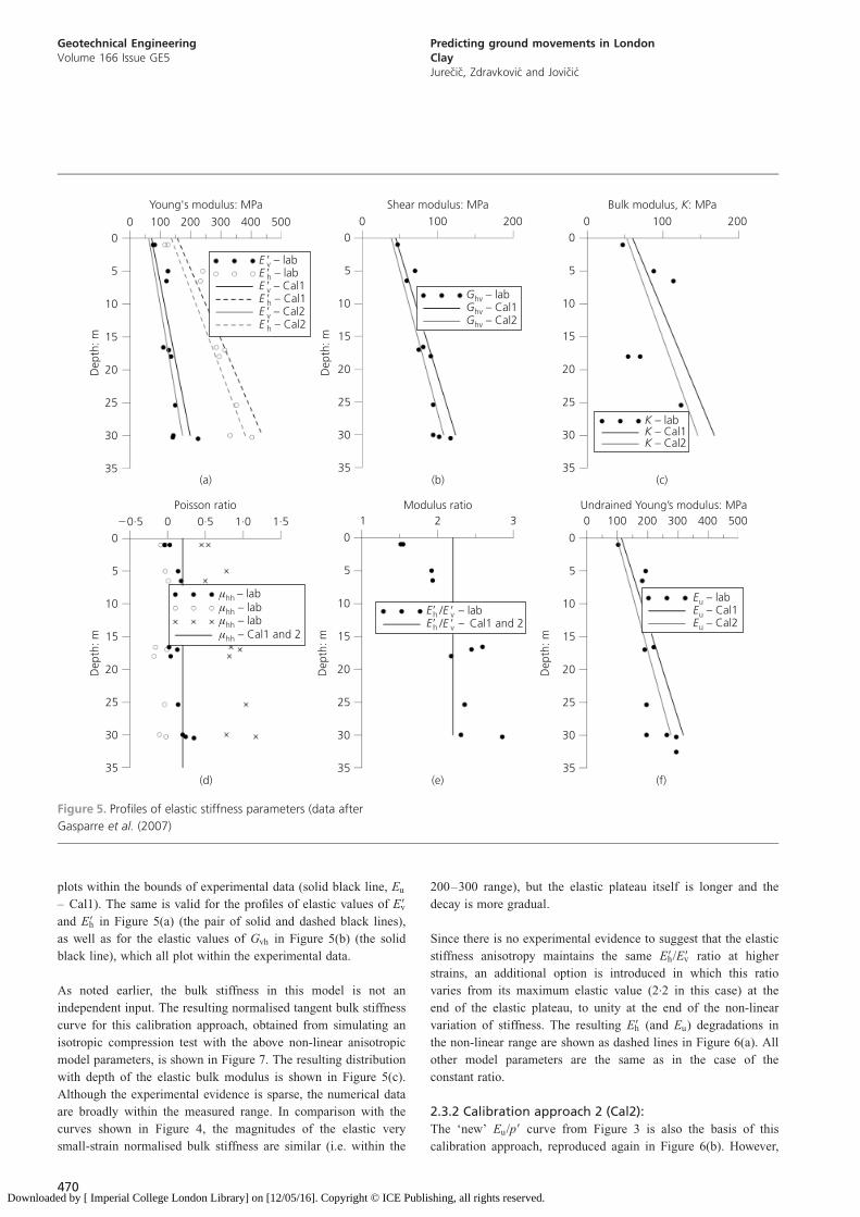
plots within the bounds of experimental data (solid black line, Eu
– Cal1). The same is valid for the profiles of elastic values of E9v
and E9h in Figure 5(a) (the pair of solid and dashed black lines),
as well as for the elastic values of Gvh in Figure 5(b) (the solid
black line), which all plot within the experimental data.
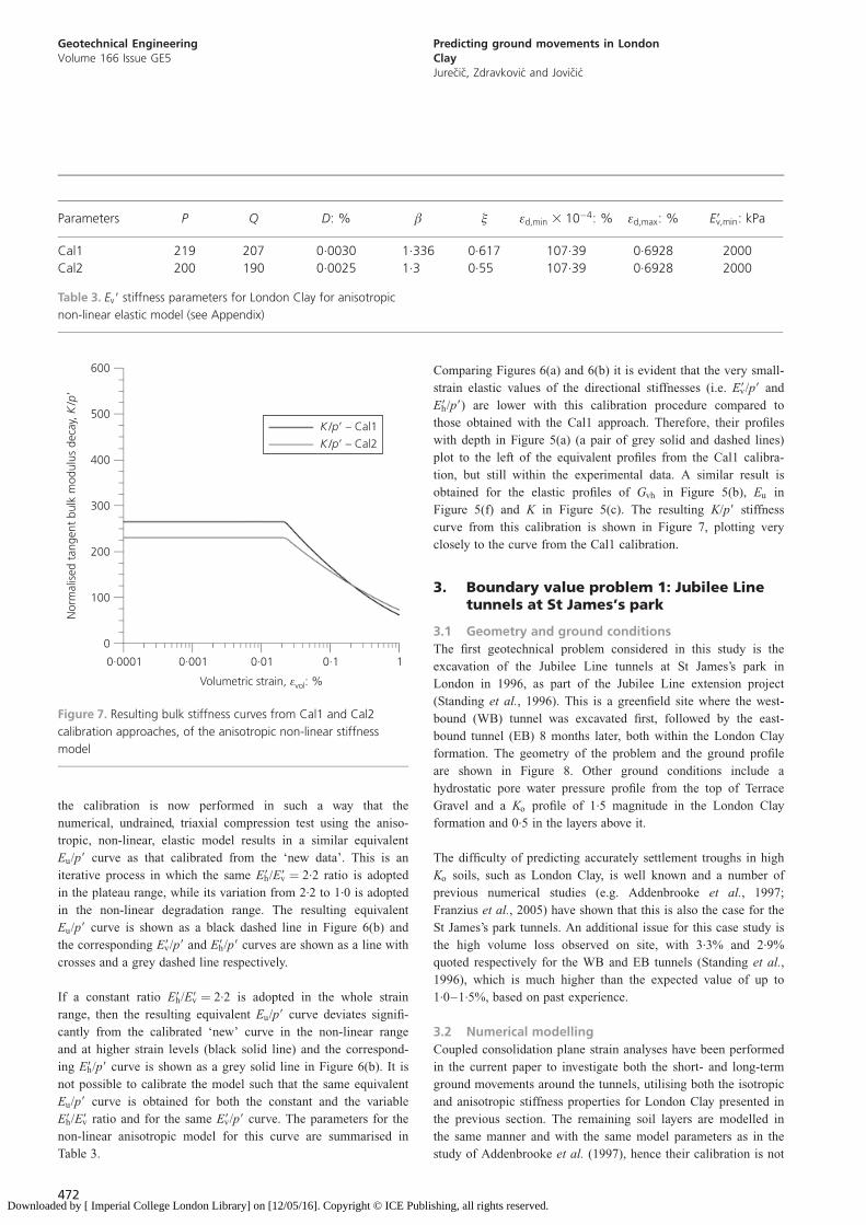
As noted earlier, the bulk stiffness in this model is not an
independent input. The resulting normalised tangent bulk stiffness
curve for this calibration approach, obtained from simulating an
isotropic compression test with the above non-linear anisotropic
model parameters, is shown in Figure 7. The resulting distribution
with depth of the elastic bulk modulus is shown in Figure 5(c).
Although the experimental evidence is sparse, the numerical data
are broadly within the measured range. In comparison with the
curves shown in Figure 4, the magnitudes of the elastic very
small-strain normalised bulk stiffness are similar (i.e. within the
200–300 range), but the elastic plateau itself is longer and the
decay is more gradual.
Since there is no experimental evidence to suggest that the elastic
stiffness anisotropy maintains the same E9h/E9v ratio at higher
strains, an additional option is introduced in which this ratio
varies from its maximum elastic value (2.2 in this case) at the
end of the elastic plateau, to unity at the end of the non-linear
variation of stiffness. The resulting E9h (and Eu) degradations in
the non-linear range are shown as dashed lines in Figure 6(a). All
other model parameters are the same as in the case of the
constant ratio.
2.3.2 Calibration approach 2 (Cal2):
The ‘new’ Eu/p9 curve from Figure 3 is also the basis of this
calibration approach, reproduced again in Figure 6(b). However,
35
30
25
20
15
10
5
0
0 100 200Undrained Young’s modulus: MPa
(f)
Eu – labEu – Cal1Eu – Cal2
35
30
25
20
15
10
5
00 100 200
Bulk modulus, : MPaK
(c)
K – labK – Cal1K – Cal2
35
30
25
20
15
10
5
00 100 200 300 400 500
Young's modulus: MPa
Dep
th: m
E �v – labE �h – labE �v – Cal1E �h – Cal1E �v – Cal2E �h – Cal2
(a)35
30
25
20
15
10
5
00 100 200
Shear modulus: MPa
Dep
th: m
(b)
Ghv – labGhv – Cal1Ghv – Cal2
/ – labE �vE�h/ – Cal1 and 2E �vE�h
Dep
th: m
300 400 500
35
30
25
20
15
10
5
00 0·5 1·0 1·5�0·5
Poisson ratio
Dep
th: m
μhh – labμhh – labμhh – labμhh Cal1 and 2–
(d)35
30
25
20
15
10
5
0
1 2 3Modulus ratio
Dep
th: m
(e)
Figure 5. Profiles of elastic stiffness parameters (data after
Gasparre et al. (2007)
470
Geotechnical EngineeringVolume 166 Issue GE5
Predicting ground movements in LondonClayJurecic, Zdravkovic and Jovicic
Downloaded by [ Imperial College London Library] on [12/05/16]. Copyright © ICE Publishing, all rights reserved.
0
100
200
300
400
500
600
700
800
0·0001 0·001 0·01 0·1 1 10
Nor
mal
ised
tan
gent
mod
ulus
dec
ay,
/,
/,
/E
pp
pu
��
�E
E�
�v
h
Deviatoric strain, : %(b)
εd
Numerical data, Cal2
E pu/ – new isotropic data�
E p� �v /
E p� �h / – constant α
E p� �h / – variable α
Equivalent / –E pu � constant α
Equivalent variable αE pu/ –�
0
100
200
300
400
500
600
700
800
0·0001 0·001 0·01 0·1 1 10
Nor
mal
ised
tan
gent
mod
ulus
dec
ay,
/,
/,
/E
pp
pu
��
�E
E�
�v
h
Deviatoric strain, : %(a)
εd
Numerical data, Cal1
E pu/ – new isotropic data�
E p� �v /
E p� �h / – constant α
E p� �h / – variable α
Equivalent / –E pu � constant α
Equivalent variable αE pu/ –�
Figure 6. Calibration for the non-linear anisotripic model:
(a) Cal1 and (b) Cal2
471
Geotechnical EngineeringVolume 166 Issue GE5
Predicting ground movements in LondonClayJurecic, Zdravkovic and Jovicic
Downloaded by [ Imperial College London Library] on [12/05/16]. Copyright © ICE Publishing, all rights reserved.
the calibration is now performed in such a way that the
numerical, undrained, triaxial compression test using the aniso-
tropic, non-linear, elastic model results in a similar equivalent
Eu/p9 curve as that calibrated from the ‘new data’. This is an
iterative process in which the same E9h/E9v ¼ 2.2 ratio is adopted
in the plateau range, while its variation from 2.2 to 1.0 is adopted
in the non-linear degradation range. The resulting equivalent
Eu/p9 curve is shown as a black dashed line in Figure 6(b) and
the corresponding E9v/p9 and E9h/p9 curves are shown as a line with
crosses and a grey dashed line respectively.
If a constant ratio E9h/E9v ¼ 2.2 is adopted in the whole strain
range, then the resulting equivalent Eu/p9 curve deviates signifi-
cantly from the calibrated ‘new’ curve in the non-linear range
and at higher strain levels (black solid line) and the correspond-
ing E9h/p9 curve is shown as a grey solid line in Figure 6(b). It is
not possible to calibrate the model such that the same equivalent
Eu/p9 curve is obtained for both the constant and the variable
E9h/E9v ratio and for the same E9v/p9 curve. The parameters for the
non-linear anisotropic model for this curve are summarised in
Table 3.
Comparing Figures 6(a) and 6(b) it is evident that the very small-
strain elastic values of the directional stiffnesses (i.e. E9v/p9 and
E9h/p9) are lower with this calibration procedure compared to
those obtained with the Cal1 approach. Therefore, their profiles
with depth in Figure 5(a) (a pair of grey solid and dashed lines)
plot to the left of the equivalent profiles from the Cal1 calibra-
tion, but still within the experimental data. A similar result is
obtained for the elastic profiles of Gvh in Figure 5(b), Eu in
Figure 5(f) and K in Figure 5(c). The resulting K/p9 stiffness
curve from this calibration is shown in Figure 7, plotting very
closely to the curve from the Cal1 calibration.
3. Boundary value problem 1: Jubilee Linetunnels at St James’s park
3.1 Geometry and ground conditions
The first geotechnical problem considered in this study is the
excavation of the Jubilee Line tunnels at St James’s park in
London in 1996, as part of the Jubilee Line extension project
(Standing et al., 1996). This is a greenfield site where the west-
bound (WB) tunnel was excavated first, followed by the east-
bound tunnel (EB) 8 months later, both within the London Clay
formation. The geometry of the problem and the ground profile
are shown in Figure 8. Other ground conditions include a
hydrostatic pore water pressure profile from the top of Terrace
Gravel and a Ko profile of 1.5 magnitude in the London Clay
formation and 0.5 in the layers above it.
The difficulty of predicting accurately settlement troughs in high
Ko soils, such as London Clay, is well known and a number of
previous numerical studies (e.g. Addenbrooke et al., 1997;
Franzius et al., 2005) have shown that this is also the case for the
St James’s park tunnels. An additional issue for this case study is
the high volume loss observed on site, with 3.3% and 2.9%
quoted respectively for the WB and EB tunnels (Standing et al.,
1996), which is much higher than the expected value of up to
1.0–1.5%, based on past experience.
3.2 Numerical modelling
Coupled consolidation plane strain analyses have been performed
in the current paper to investigate both the short- and long-term
ground movements around the tunnels, utilising both the isotropic
and anisotropic stiffness properties for London Clay presented in
the previous section. The remaining soil layers are modelled in
the same manner and with the same model parameters as in the
study of Addenbrooke et al. (1997), hence their calibration is not
Parameters P Q D: % � � �d,min 3 10�4: % �d,max: % E9v,min: kPa
Cal1 219 207 0.0030 1.336 0.617 107.39 0.6928 2000
Cal2 200 190 0.0025 1.3 0.55 107.39 0.6928 2000
Table 3. Ev9 stiffness parameters for London Clay for anisotropic
non-linear elastic model (see Appendix)
0
100
200
300
400
500
600
0·0001 0·001 0·01 0·1 1
Nor
mal
ised
tan
gent
bul
k m
odul
us d
ecay
,/
Kp�
Volumetric strain, : %εvol
K p/ – Cal1�
K p/ – Cal2�
Figure 7. Resulting bulk stiffness curves from Cal1 and Cal2
calibration approaches, of the anisotropic non-linear stiffness
model
472
Geotechnical EngineeringVolume 166 Issue GE5
Predicting ground movements in LondonClayJurecic, Zdravkovic and Jovicic
Downloaded by [ Imperial College London Library] on [12/05/16]. Copyright © ICE Publishing, all rights reserved.
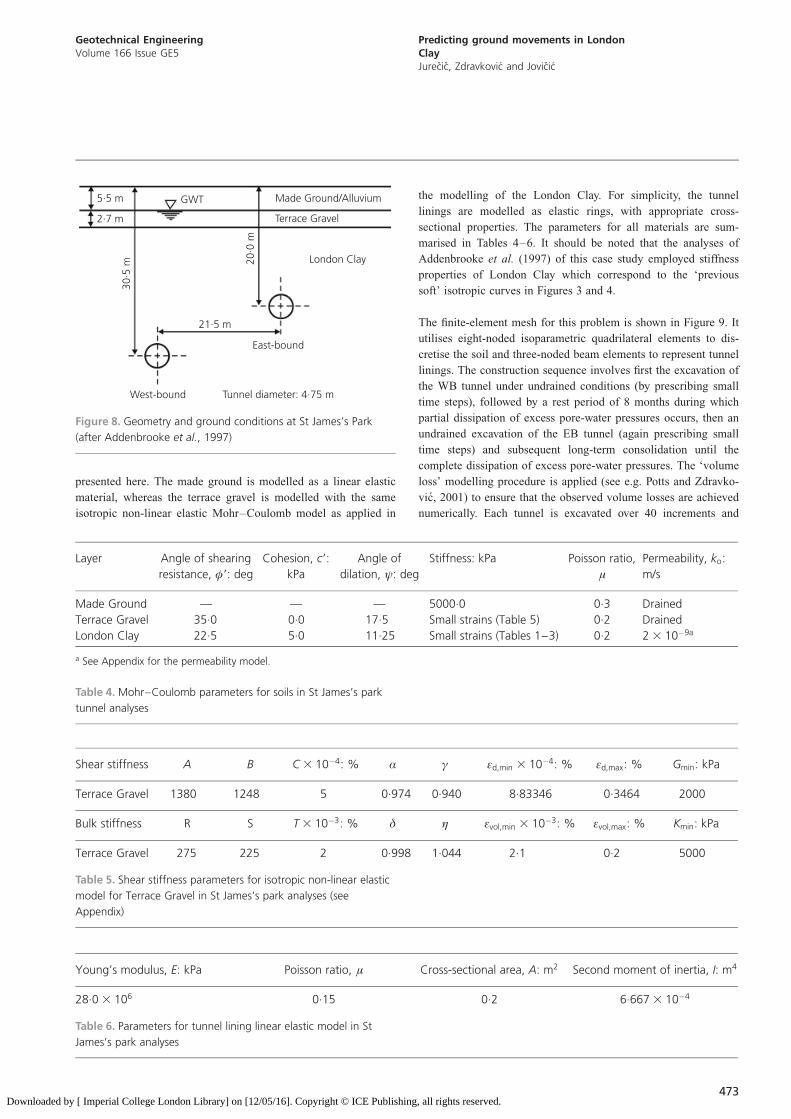
presented here. The made ground is modelled as a linear elastic
material, whereas the terrace gravel is modelled with the same
isotropic non-linear elastic Mohr–Coulomb model as applied in
the modelling of the London Clay. For simplicity, the tunnel
linings are modelled as elastic rings, with appropriate cross-
sectional properties. The parameters for all materials are sum-
marised in Tables 4–6. It should be noted that the analyses of
Addenbrooke et al. (1997) of this case study employed stiffness
properties of London Clay which correspond to the ‘previous
soft’ isotropic curves in Figures 3 and 4.
The finite-element mesh for this problem is shown in Figure 9. It
utilises eight-noded isoparametric quadrilateral elements to dis-
cretise the soil and three-noded beam elements to represent tunnel
linings. The construction sequence involves first the excavation of
the WB tunnel under undrained conditions (by prescribing small
time steps), followed by a rest period of 8 months during which
partial dissipation of excess pore-water pressures occurs, then an
undrained excavation of the EB tunnel (again prescribing small
time steps) and subsequent long-term consolidation until the
complete dissipation of excess pore-water pressures. The ‘volume
loss’ modelling procedure is applied (see e.g. Potts and Zdravko-
vic, 2001) to ensure that the observed volume losses are achieved
numerically. Each tunnel is excavated over 40 increments and
5·5 m
2·7 m
GWT
30·5
m 20·0
m
Made Ground/Alluvium
Terrace Gravel
London Clay
21·5 m
West-bound
East-bound
Tunnel diameter: 4·75 m
Figure 8. Geometry and ground conditions at St James’s Park
(after Addenbrooke et al., 1997)
Layer Angle of shearing
resistance, �9: deg
Cohesion, c9:
kPa
Angle of
dilation, ł: deg
Stiffness: kPa Poisson ratio,
�Permeability, ko:
m/s
Made Ground — — — 5000.0 0.3 Drained
Terrace Gravel 35.0 0.0 17.5 Small strains (Table 5) 0.2 Drained
London Clay 22.5 5.0 11.25 Small strains (Tables 1–3) 0.2 2 3 10�9a
a See Appendix for the permeability model.
Table 4. Mohr–Coulomb parameters for soils in St James’s park
tunnel analyses
Shear stiffness A B C 3 10�4: % Æ ª �d,min 3 10�4: % �d,max: % Gmin: kPa
Terrace Gravel 1380 1248 5 0.974 0.940 8.83346 0.3464 2000
Bulk stiffness R S T 3 10�3: % � � �vol,min 3 10�3: % �vol,max: % Kmin: kPa
Terrace Gravel 275 225 2 0.998 1.044 2.1 0.2 5000
Table 5. Shear stiffness parameters for isotropic non-linear elastic
model for Terrace Gravel in St James’s park analyses (see
Appendix)
Young’s modulus, E: kPa Poisson ratio, � Cross-sectional area, A: m2 Second moment of inertia, I: m4
28.0 3 106 0.15 0.2 6.667 3 10�4
Table 6. Parameters for tunnel lining linear elastic model in St
James’s park analyses
473
Geotechnical EngineeringVolume 166 Issue GE5
Predicting ground movements in LondonClayJurecic, Zdravkovic and Jovicic
Downloaded by [ Imperial College London Library] on [12/05/16]. Copyright © ICE Publishing, all rights reserved.
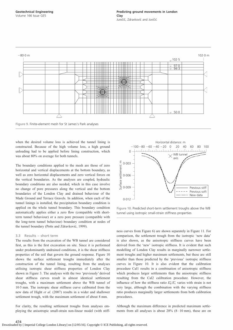
when the desired volume loss is achieved the tunnel lining is
constructed. Because of the high volume loss, a high ground
unloading had to be applied before lining construction, which
was about 80% on average for both tunnels.
The boundary conditions applied to the mesh are those of zero
horizontal and vertical displacements at the bottom boundary, as
well as zero horizontal displacements and zero vertical forces on
the vertical boundaries. As the analyses are coupled, hydraulic
boundary conditions are also needed, which in this case involve
no change of pore pressures along the vertical and the bottom
boundaries of the London Clay and drained behaviour of the
Made Ground and Terrace Gravels. In addition, when each of the
tunnel linings is installed, the precipitation boundary condition is
applied on the whole tunnel boundary. This boundary condition
automatically applies either a zero flow (compatible with short-
term tunnel behaviour) or a zero pore pressure (compatible with
the long-term tunnel behaviour) boundary condition at nodes of
the tunnel boundary (Potts and Zdravkovic, 1999).
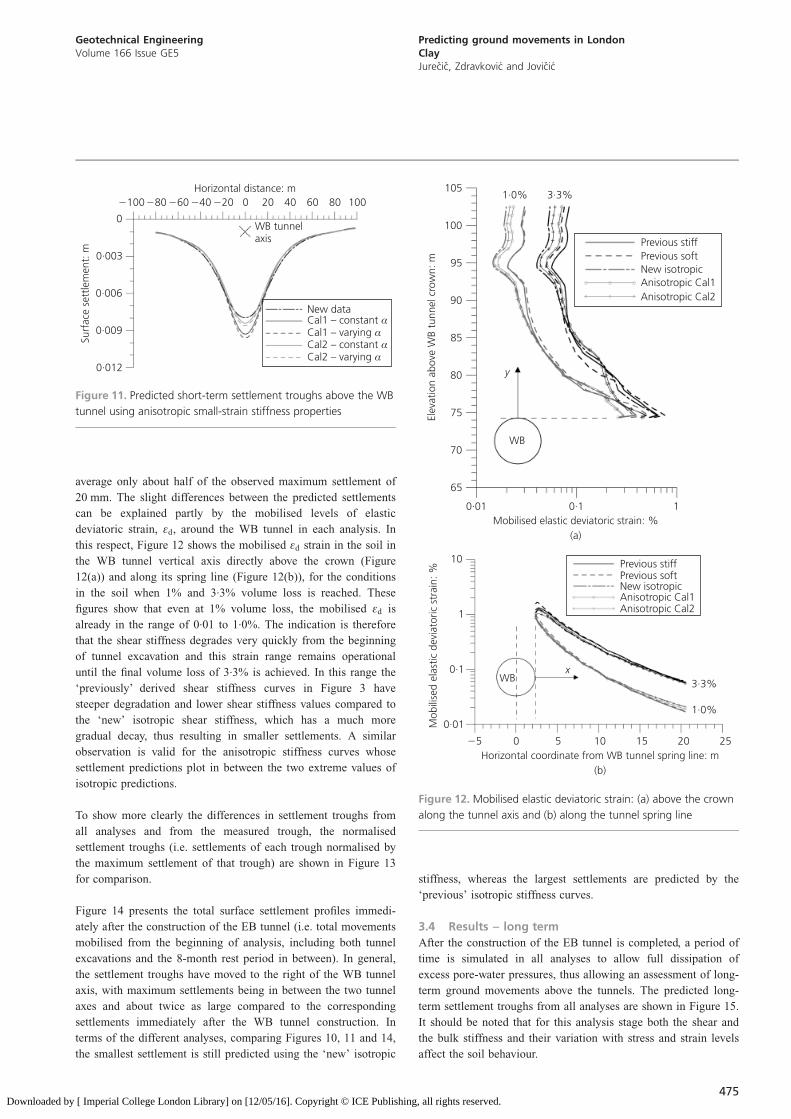
3.3 Results – short term
The results from the excavation of the WB tunnel are considered
first, as this is the first excavation on site. Since it is performed
under predominantly undrained conditions, it is the shear stiffness
properties of the soil that govern the ground response. Figure 10
shows the surface settlement troughs immediately after the
construction of the tunnel lining, resulting from the analyses
utilising isotropic shear stiffness properties of London Clay
shown in Figure 3. The analyses with the two ‘previously’ derived
shear stiffness curves result in almost identical settlement
troughs, with a maximum settlement above the WB tunnel of
10.5 mm. The isotropic shear stiffness curve calibrated from the
new data of Hight et al. (2007) results in a wider and shallower
settlement trough, with the maximum settlement of about 8 mm.
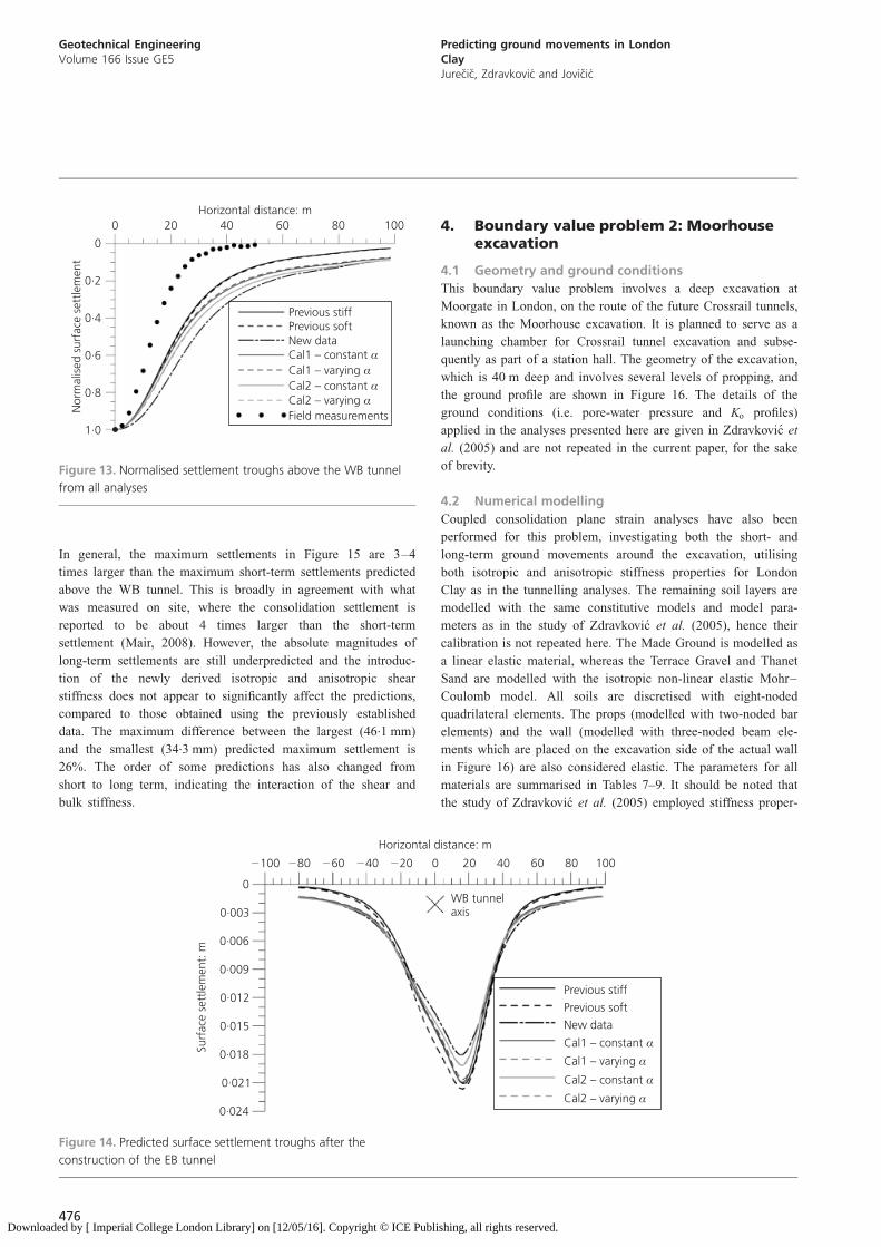
For clarity, the resulting settlement troughs from analyses em-
ploying the anisotropic small-strain non-linear model (with stiff-
ness curves from Figure 6) are shown separately in Figure 11. For
comparison, the settlement trough from the isotropic ‘new data’
is also shown, as the anisotropic stiffness curves have been
derived from the ‘new’ isotropic stiffness. It is evident that such
modelling of London Clay results in marginally narrower settle-
ment troughs and higher maximum settlements, but these are still
smaller than those predicted by the ‘previous’ isotropic stiffness
curves in Figure 10. It is also evident that the calibration
procedure Cal1 results in a combination of anisotropic stiffness
which produces larger settlements than the anisotropic stiffness
resulting from the Cal2 calibration procedure. However, the
influence of how the stiffness ratio E9h/E9v varies with strain is not
very large, although the combination with the varying stiffness
ratio produces marginally larger settlements from both calibration
procedures.
Although the maximum difference in predicted maximum settle-
ments from all analyses is about 20% (8–10 mm), these are on
�80·0 m102·5
102·0 m
97·094·3
50·0
Figure 9. Finite-element mesh for St James’s Park analyses
0·012
0·009
0·006
0·003
0
�100�80 �60 �40 �20 0 20 40 60 80 100Horizontal distance: m
Surf
ace
sett
lem
ent:
m
Previous stiffPrevious softNew data
WB tunnelaxis
Figure 10. Predicted short-term settlement troughs above the WB
tunnel using isotropic small-strain stiffness properties
474
Geotechnical EngineeringVolume 166 Issue GE5
Predicting ground movements in LondonClayJurecic, Zdravkovic and Jovicic
Downloaded by [ Imperial College London Library] on [12/05/16]. Copyright © ICE Publishing, all rights reserved.
average only about half of the observed maximum settlement of
20 mm. The slight differences between the predicted settlements
can be explained partly by the mobilised levels of elastic
deviatoric strain, �d, around the WB tunnel in each analysis. In
this respect, Figure 12 shows the mobilised �d strain in the soil in
the WB tunnel vertical axis directly above the crown (Figure
12(a)) and along its spring line (Figure 12(b)), for the conditions
in the soil when 1% and 3.3% volume loss is reached. These
figures show that even at 1% volume loss, the mobilised �d is
already in the range of 0.01 to 1.0%. The indication is therefore
that the shear stiffness degrades very quickly from the beginning
of tunnel excavation and this strain range remains operational
until the final volume loss of 3.3% is achieved. In this range the
‘previously’ derived shear stiffness curves in Figure 3 have
steeper degradation and lower shear stiffness values compared to
the ‘new’ isotropic shear stiffness, which has a much more
gradual decay, thus resulting in smaller settlements. A similar
observation is valid for the anisotropic stiffness curves whose
settlement predictions plot in between the two extreme values of
isotropic predictions.
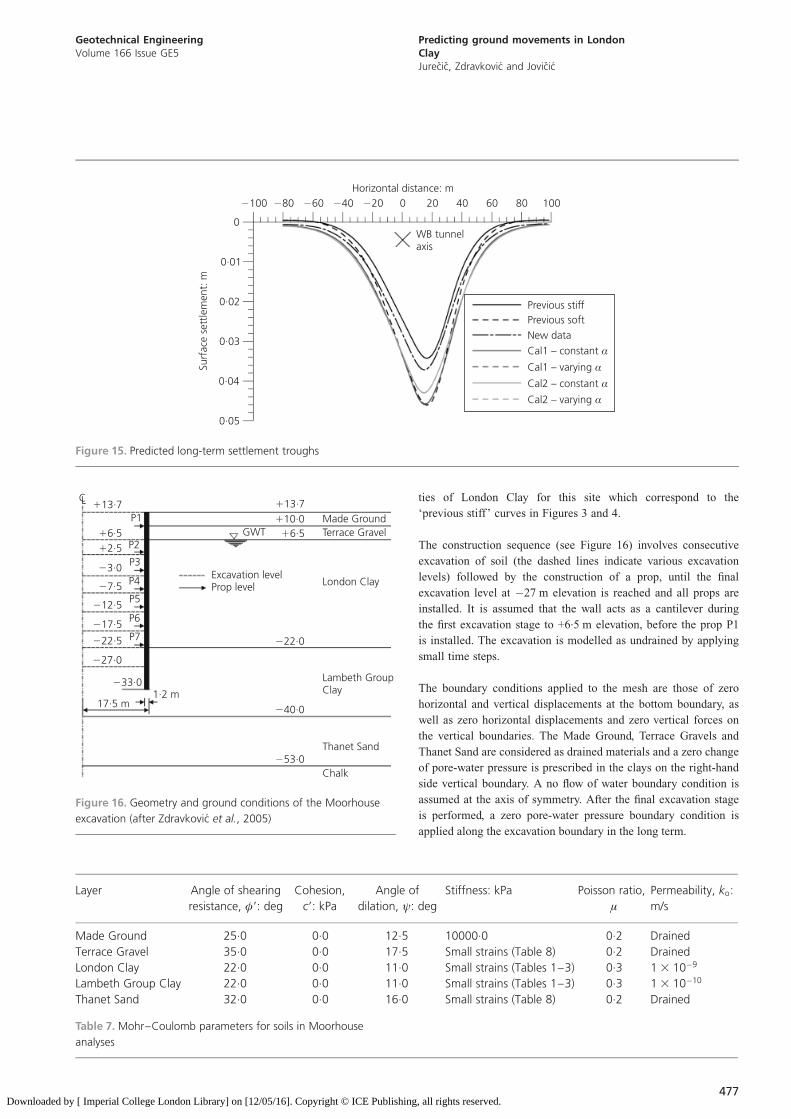
To show more clearly the differences in settlement troughs from
all analyses and from the measured trough, the normalised
settlement troughs (i.e. settlements of each trough normalised by
the maximum settlement of that trough) are shown in Figure 13
for comparison.
Figure 14 presents the total surface settlement profiles immedi-
ately after the construction of the EB tunnel (i.e. total movements
mobilised from the beginning of analysis, including both tunnel
excavations and the 8-month rest period in between). In general,
the settlement troughs have moved to the right of the WB tunnel
axis, with maximum settlements being in between the two tunnel
axes and about twice as large compared to the corresponding
settlements immediately after the WB tunnel construction. In
terms of the different analyses, comparing Figures 10, 11 and 14,
the smallest settlement is still predicted using the ‘new’ isotropic
stiffness, whereas the largest settlements are predicted by the
‘previous’ isotropic stiffness curves.
3.4 Results – long term
After the construction of the EB tunnel is completed, a period of
time is simulated in all analyses to allow full dissipation of
excess pore-water pressures, thus allowing an assessment of long-
term ground movements above the tunnels. The predicted long-
term settlement troughs from all analyses are shown in Figure 15.
It should be noted that for this analysis stage both the shear and
the bulk stiffness and their variation with stress and strain levels
affect the soil behaviour.
0·012
0·009
0·006
0·003
0
�100�80 �60 �40 �20 0 20 40 60 80 100Horizontal distance: m
Surf
ace
sett
lem
ent:
m
Cal1 – constant αNew data
WB tunnelaxis
Cal1 – varying αCal2 – constant αCal2 – αvarying
Figure 11. Predicted short-term settlement troughs above the WB
tunnel using anisotropic small-strain stiffness properties
105
100
95
90
85
80
75
70
65
Elev
atio
n ab
ove
WB
tunn
el c
r ow
n: m
0·01 0·1 1Mobilised elastic deviatoric strain: %
(a)
WB
y
Previous stiffPrevious softNew isotropicAnisotropic Cal1Anisotropic Cal2
Previous stiffPrevious softNew isotropicAnisotropic Cal1Anisotropic Cal2
WBx
Mob
ilise
d el
astic
dev
iato
ric s
trai
n: %
10
1
0·1
0·01
�5 0 5 10 15 20 25
3·3%
1·0%
Horizontal coordinate from WB tunnel spring line: m(b)
1·0% 3·3%
Figure 12. Mobilised elastic deviatoric strain: (a) above the crown
along the tunnel axis and (b) along the tunnel spring line
475
Geotechnical EngineeringVolume 166 Issue GE5
Predicting ground movements in LondonClayJurecic, Zdravkovic and Jovicic
Downloaded by [ Imperial College London Library] on [12/05/16]. Copyright © ICE Publishing, all rights reserved.
In general, the maximum settlements in Figure 15 are 3–4
times larger than the maximum short-term settlements predicted
above the WB tunnel. This is broadly in agreement with what
was measured on site, where the consolidation settlement is
reported to be about 4 times larger than the short-term
settlement (Mair, 2008). However, the absolute magnitudes of
long-term settlements are still underpredicted and the introduc-
tion of the newly derived isotropic and anisotropic shear
stiffness does not appear to significantly affect the predictions,
compared to those obtained using the previously established
data. The maximum difference between the largest (46.1 mm)
and the smallest (34.3 mm) predicted maximum settlement is
26%. The order of some predictions has also changed from
short to long term, indicating the interaction of the shear and
bulk stiffness.
4. Boundary value problem 2: Moorhouseexcavation
4.1 Geometry and ground conditions
This boundary value problem involves a deep excavation at
Moorgate in London, on the route of the future Crossrail tunnels,
known as the Moorhouse excavation. It is planned to serve as a
launching chamber for Crossrail tunnel excavation and subse-
quently as part of a station hall. The geometry of the excavation,
which is 40 m deep and involves several levels of propping, and
the ground profile are shown in Figure 16. The details of the
ground conditions (i.e. pore-water pressure and Ko profiles)
applied in the analyses presented here are given in Zdravkovic et
al. (2005) and are not repeated in the current paper, for the sake
of brevity.
4.2 Numerical modelling
Coupled consolidation plane strain analyses have also been
performed for this problem, investigating both the short- and
long-term ground movements around the excavation, utilising
both isotropic and anisotropic stiffness properties for London
Clay as in the tunnelling analyses. The remaining soil layers are
modelled with the same constitutive models and model para-
meters as in the study of Zdravkovic et al. (2005), hence their
calibration is not repeated here. The Made Ground is modelled as
a linear elastic material, whereas the Terrace Gravel and Thanet
Sand are modelled with the isotropic non-linear elastic Mohr–
Coulomb model. All soils are discretised with eight-noded
quadrilateral elements. The props (modelled with two-noded bar
elements) and the wall (modelled with three-noded beam ele-
ments which are placed on the excavation side of the actual wall
in Figure 16) are also considered elastic. The parameters for all
materials are summarised in Tables 7–9. It should be noted that
the study of Zdravkovic et al. (2005) employed stiffness proper-
1·0
0·8
0·6
0·4
0·2
0
0 20 40 60 80 100Horizontal distance: m
Nor
mal
ised
sur
face
set
tlem
ent
Cal1 – constant αNew data
Cal1 – varying αCal2 – constant αCal2 – αvaryingField measurements
Previous stiffPrevious soft
Figure 13. Normalised settlement troughs above the WB tunnel
from all analyses
0·012
0·009
0·006
0·003
0
�100 �80 �60 �40 �20 0 20 40 60 80 100
Horizontal distance: m
Surf
ace
sett
lem
ent:
m
Cal1 – constant αNew data
WB tunnelaxis
Cal1 – varying α
Cal2 – constant α
Cal2 – αvarying
0·015
0·018
0·021
0·024
Previous stiff
Previous soft
Figure 14. Predicted surface settlement troughs after the
construction of the EB tunnel
476
Geotechnical EngineeringVolume 166 Issue GE5
Predicting ground movements in LondonClayJurecic, Zdravkovic and Jovicic
Downloaded by [ Imperial College London Library] on [12/05/16]. Copyright © ICE Publishing, all rights reserved.
ties of London Clay for this site which correspond to the
‘previous stiff’ curves in Figures 3 and 4.
The construction sequence (see Figure 16) involves consecutive
excavation of soil (the dashed lines indicate various excavation
levels) followed by the construction of a prop, until the final
excavation level at �27 m elevation is reached and all props are
installed. It is assumed that the wall acts as a cantilever during
the first excavation stage to +6.5 m elevation, before the prop P1
is installed. The excavation is modelled as undrained by applying
small time steps.
The boundary conditions applied to the mesh are those of zero
horizontal and vertical displacements at the bottom boundary, as
well as zero horizontal displacements and zero vertical forces on
the vertical boundaries. The Made Ground, Terrace Gravels and
Thanet Sand are considered as drained materials and a zero change
of pore-water pressure is prescribed in the clays on the right-hand
side vertical boundary. A no flow of water boundary condition is
assumed at the axis of symmetry. After the final excavation stage
is performed, a zero pore-water pressure boundary condition is
applied along the excavation boundary in the long term.
0·04
0·03
0·02
0·01
0
�100 �80 �60 �40 �20 0 20 40 60 80 100Horizontal distance: m
Surf
ace
sett
lem
ent:
m
Cal1 – constant αNew data
WB tunnelaxis
Cal1 – varying α
Cal2 – constant αCal2 – αvarying
0·05
Previous stiffPrevious soft
Figure 15. Predicted long-term settlement troughs
CL �13·7P1
�6·5P2�2·5P3
�3·0P4
�7·5P5
�12·5P6
�17·5P7�22·5
�27·0
�33·0
17·5 m1·2 m
GWT
Excavation levelProp level
�13·7�10·0
�6·5
�22·0
�40·0
�53·0
Made GroundTerrace Gravel
London Clay
Lambeth GroupClay
Thanet Sand
Chalk
Figure 16. Geometry and ground conditions of the Moorhouse
excavation (after Zdravkovic et al., 2005)
Layer Angle of shearing
resistance, �9: deg
Cohesion,
c9: kPa
Angle of
dilation, ł: deg
Stiffness: kPa Poisson ratio,
�Permeability, ko:
m/s
Made Ground 25.0 0.0 12.5 10000.0 0.2 Drained
Terrace Gravel 35.0 0.0 17.5 Small strains (Table 8) 0.2 Drained
London Clay 22.0 0.0 11.0 Small strains (Tables 1–3) 0.3 1 3 10�9
Lambeth Group Clay 22.0 0.0 11.0 Small strains (Tables 1–3) 0.3 1 3 10�10
Thanet Sand 32.0 0.0 16.0 Small strains (Table 8) 0.2 Drained
Table 7. Mohr–Coulomb parameters for soils in Moorhouse
analyses
477
Geotechnical EngineeringVolume 166 Issue GE5
Predicting ground movements in LondonClayJurecic, Zdravkovic and Jovicic
Downloaded by [ Imperial College London Library] on [12/05/16]. Copyright © ICE Publishing, all rights reserved.
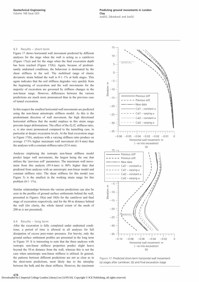
4.3 Results – short term
Figure 17 shows horizontal wall movement predicted by different
analyses for the stage when the wall is acting as a cantilever
(Figure 17(a)) and for the stage when the final excavation depth
has been reached (Figure 17(b)). Again, because of predomi-
nantly undrained conditions, the behaviour is dominated by the
shear stiffness in the soil. The mobilised range of elastic
deviatoric strain behind the wall is 0.1–1% at both stages. This
again indicates that the soil stiffness degrades very quickly from
the beginning of excavation and the wall movements for the
majority of excavation are governed by stiffness changes in the
non-linear range. However, differences between the various
predictions are much more pronounced than in the previous case
of tunnel excavation.
In this respect the smallest horizontal wall movements are predicted
using the non-linear anisotropic stiffness model. As this is the
predominant direction of wall movement, the high directional
horizontal stiffness that the model employs in this strain range
prevents larger deformations. The effect of the E9h/E9v stiffness ratio,
Æ, is also more pronounced compared to the tunnelling case, in
particular at deeper excavation levels. At the final excavation stage
in Figure 17(b), analyses with a varying stiffness ratio produce on
average 17.5% higher maximum wall movement (61.8 mm) than
the analyses with a constant stiffness ratio (52.6 mm).
Analyses employing the isotropic non-linear stiffness model
predict larger wall movements, the largest being the one that
utilises the ‘previous soft’ parameters. The maximum wall move-
ment from this analysis (95.4 mm) is 80% higher than that
predicted from analyses with an anisotropic non-linear model and
constant stiffness ratio. The shear stiffness for this model (see
Figure 3) is the smallest in the working strain range for this
problem (0.1–1%).
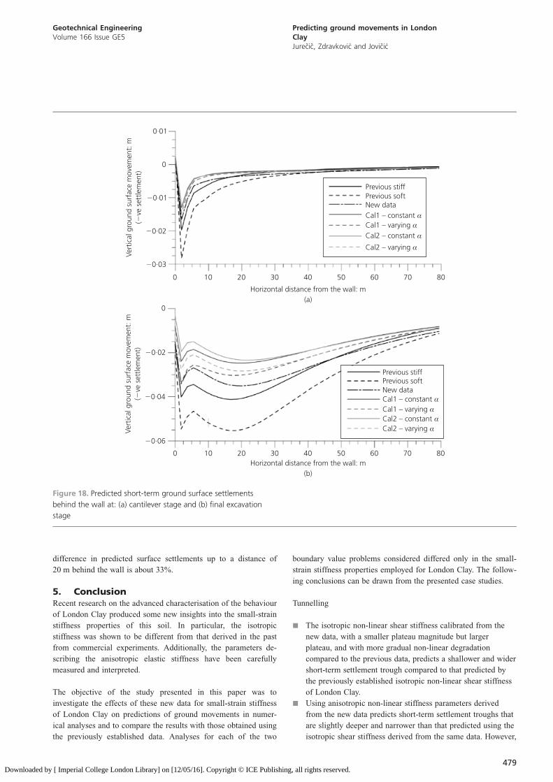
Similar relationships between the various predictions can also be
seen in the profiles of ground surface settlements behind the wall,
presented in Figures 18(a) and 18(b) for the cantilever and final
stage of excavation respectively, and for the 80 m distance behind
the wall (for clarity, the whole lateral extent of the mesh of
200 m is not presented).
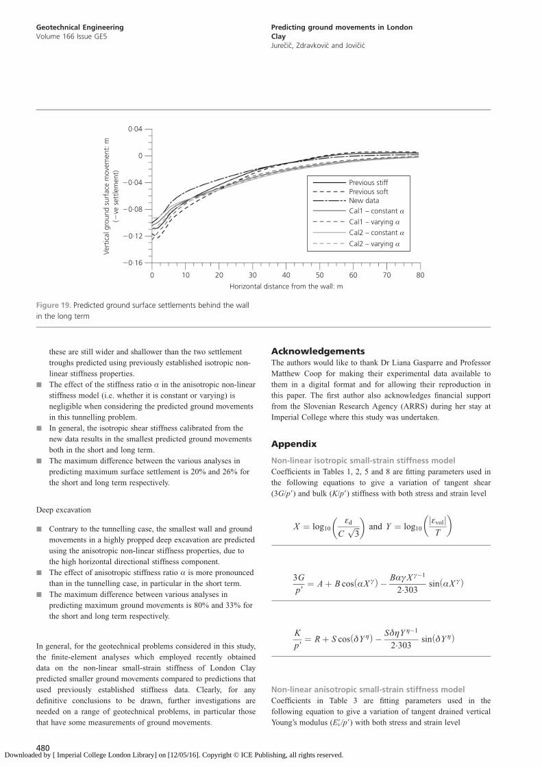
4.4 Results – long term
After the excavation is fully completed under undrained condi-
tions, a period of time is allowed in all analyses for full
dissipation of excess pore-water pressures. For brevity, only the
ground surface settlement profiles are presented in the long term
in Figure 19. It is interesting to note that the three analyses with
isotropic non-linear stiffness properties predict slight heave
beyond the 50 m distance from the wall, whereas this is not the
case when anisotropic non-linear stiffness is utilised. In general,
the patterns between different predictions are not as clear as in
the short-term predictions, most likely due to the interplay
between the bulk and the shear stiffness. However, the maximum
�35
�30
�25
�20
�15
�10
�5
15
�0·10 �0·08 �0·06 �0·04 �0·02 0
Elev
atio
n: m
Horizontal wall movement: m( ve into excavation)
(b)�
Cal1 – constant αNew data
Cal1 – varying α
Cal2 – constant α
Cal2 – αvarying
Previous stiffPrevious soft
�35
�30
�25
�20
�15
�10
�5
0
5
10
15
�0·06 �0·05 �0·04 �0·03 �0·02 �0·01 0
Elev
atio
n: m
Horizontal wall movement: m( ve into excavation)
(a)�
Cal1 – constant α
New data
Cal1 – varying α
Cal2 – constant α
Cal2 – αvarying
Previous stiff
Previous soft
Figure 17. Predicted short-term horizontal wall movement:
(a) stages after cantilever; (b) and final excavation stage
478
Geotechnical EngineeringVolume 166 Issue GE5
Predicting ground movements in LondonClayJurecic, Zdravkovic and Jovicic
Downloaded by [ Imperial College London Library] on [12/05/16]. Copyright © ICE Publishing, all rights reserved.
difference in predicted surface settlements up to a distance of
20 m behind the wall is about 33%.
5. ConclusionRecent research on the advanced characterisation of the behaviour
of London Clay produced some new insights into the small-strain
stiffness properties of this soil. In particular, the isotropic
stiffness was shown to be different from that derived in the past
from commercial experiments. Additionally, the parameters de-
scribing the anisotropic elastic stiffness have been carefully
measured and interpreted.
The objective of the study presented in this paper was to
investigate the effects of these new data for small-strain stiffness
of London Clay on predictions of ground movements in numer-
ical analyses and to compare the results with those obtained using
the previously established data. Analyses for each of the two
boundary value problems considered differed only in the small-
strain stiffness properties employed for London Clay. The follow-
ing conclusions can be drawn from the presented case studies.
Tunnelling
j The isotropic non-linear shear stiffness calibrated from the
new data, with a smaller plateau magnitude but larger
plateau, and with more gradual non-linear degradation
compared to the previous data, predicts a shallower and wider
short-term settlement trough compared to that predicted by
the previously established isotropic non-linear shear stiffness
of London Clay.
j Using anisotropic non-linear stiffness parameters derived
from the new data predicts short-term settlement troughs that
are slightly deeper and narrower than that predicted using the
isotropic shear stiffness derived from the same data. However,
�0·03
0
0 20 30 40 50 60
Vert
ical
gro
und
surf
ace
mov
emen
t: m
(ve
set
tlem
ent)
�
Cal1 – constant αNew data
Cal1 – varying αCal2 – constant α
Cal2 – αvarying
Previous stiffPrevious soft
10 70 80
Horizontal distance from the wall: m(a)
�0·02
�0·01
0·01
�0·06
0
0 20 30 40 50 60
Vert
ical
gro
und
surf
ace
mov
emen
t: m
(ve
set
tlem
ent)
� Cal1 – constant αNew data
Cal1 – varying αCal2 – constant αCal2 – αvarying
Previous stiffPrevious soft
10 70 80Horizontal distance from the wall: m
(b)
�0·04
�0·02
Figure 18. Predicted short-term ground surface settlements
behind the wall at: (a) cantilever stage and (b) final excavation
stage
479
Geotechnical EngineeringVolume 166 Issue GE5
Predicting ground movements in LondonClayJurecic, Zdravkovic and Jovicic
Downloaded by [ Imperial College London Library] on [12/05/16]. Copyright © ICE Publishing, all rights reserved.
these are still wider and shallower than the two settlement
troughs predicted using previously established isotropic non-
linear stiffness properties.
j The effect of the stiffness ratio Æ in the anisotropic non-linear
stiffness model (i.e. whether it is constant or varying) is
negligible when considering the predicted ground movements
in this tunnelling problem.
j In general, the isotropic shear stiffness calibrated from the
new data results in the smallest predicted ground movements
both in the short and long term.
j The maximum difference between the various analyses in
predicting maximum surface settlement is 20% and 26% for
the short and long term respectively.
Deep excavation
j Contrary to the tunnelling case, the smallest wall and ground
movements in a highly propped deep excavation are predicted
using the anisotropic non-linear stiffness properties, due to
the high horizontal directional stiffness component.
j The effect of anisotropic stiffness ratio Æ is more pronounced
than in the tunnelling case, in particular in the short term.
j The maximum difference between various analyses in
predicting maximum ground movements is 80% and 33% for
the short and long term respectively.
In general, for the geotechnical problems considered in this study,
the finite-element analyses which employed recently obtained
data on the non-linear small-strain stiffness of London Clay
predicted smaller ground movements compared to predictions that
used previously established stiffness data. Clearly, for any
definitive conclusions to be drawn, further investigations are
needed on a range of geotechnical problems, in particular those
that have some measurements of ground movements.
AcknowledgementsThe authors would like to thank Dr Liana Gasparre and Professor
Matthew Coop for making their experimental data available to
them in a digital format and for allowing their reproduction in
this paper. The first author also acknowledges financial support
from the Slovenian Research Agency (ARRS) during her stay at
Imperial College where this study was undertaken.
Appendix
Non-linear isotropic small-strain stiffness model
Coefficients in Tables 1, 2, 5 and 8 are fitting parameters used in
the following equations to give a variation of tangent shear
(3G/p9) and bulk (K/p9) stiffness with both stress and strain level
X ¼ log10
�d
Cffiffiffi3p
� �and Y ¼ log10
�volj jT
� �
3G
p9¼ Aþ B cos ÆX ªð Þ � BƪX ª�1
2:303sin ÆX ªð Þ
K
p9¼ Rþ S cos �Y �ð Þ � S��Y ��1
2:303sin �Y �ð Þ
Non-linear anisotropic small-strain stiffness model
Coefficients in Table 3 are fitting parameters used in the
following equation to give a variation of tangent drained vertical
Young’s modulus (E9v/p9) with both stress and strain level
�0·16
0
0 20 30 40 50 60
Vert
ical
gro
und
surf
ace
mov
emen
t: m
(ve
set
tlem
ent)
�
Cal1 – constant αNew data
Cal1 – varying αCal2 – constant α
Cal2 – αvarying
Previous stiffPrevious soft
10 70 80
Horizontal distance from the wall: m
�0·08
�0·04
0·04
�0·12
Figure 19. Predicted ground surface settlements behind the wall
in the long term
480
Geotechnical EngineeringVolume 166 Issue GE5
Predicting ground movements in LondonClayJurecic, Zdravkovic and Jovicic
Downloaded by [ Imperial College London Library] on [12/05/16]. Copyright © ICE Publishing, all rights reserved.
Z ¼ log10
�d
Dffiffiffi3p
� �
E9v
p9¼ Pþ Q cos �Z�
� �� Q��Z��1
2:303sin �Z�� �
Using input parameters E9v, �9hh and Æ, the remaining cross-
anisotropic elastic parameters are calculated as (Graham and
Houlsby, 1983)
E9h ¼ Æ2E9v
Ghv ¼Æ E9v
2 1þ �9hhð Þ
Ghh ¼E9h
2 1þ �9hhð Þ
�9vh ¼ �9hh=Æ
�9hv ¼ �9vh
E9h
E9y
Permeability model
The coefficient of permeability k is assumed to be related to the
mean effective stress p9 through the following equation (Vaughan,
1994)
k ¼ ko e�ap9
where for London Clay a ¼ 0.007 and ko ¼ 2 3 10�9 m/s.
REFERENCES
Addenbrooke TI, Potts DM and Puzrin AM (1997) The influence
of pre-failure soil stiffness on the numerical analysis of
tunnel construction. Geotechnique 47(3): 693–712.
Baudet B and Stallebrass S (2004) A constitutive model for
structured clays. Geotechnique 54(4): 269–278.
Franzius JN, Potts DM and Burland JB (2005) The influence of
soil anisotropy and Ko on ground surface movements resulting
from tunnel excavation. Geotechnique 55(3): 189–199.
Gasparre A (2005) Advanced Laboratory Characterisation of
London Clay. PhD thesis, Imperial College London, UK.
Gasparre A, Nishimura S, Minh NA, Coop MR and Jardine RJ
(2007) The stiffness of natural London Clay. Geotechnique
57(1): 33–47.
Graham J and Houlsby GT (1983) Anisotropic elasticity of a
natural clay. Geotechnique 33(2): 165–180.
Grammatikopoulou A, Zdravkovic L and Potts DM (2006)
General formulation of two kinematic hardening constitutive
models with a smooth elasto-plastic transition. International
Journal of Geomechanics, ASCE 6(5): 291–302.
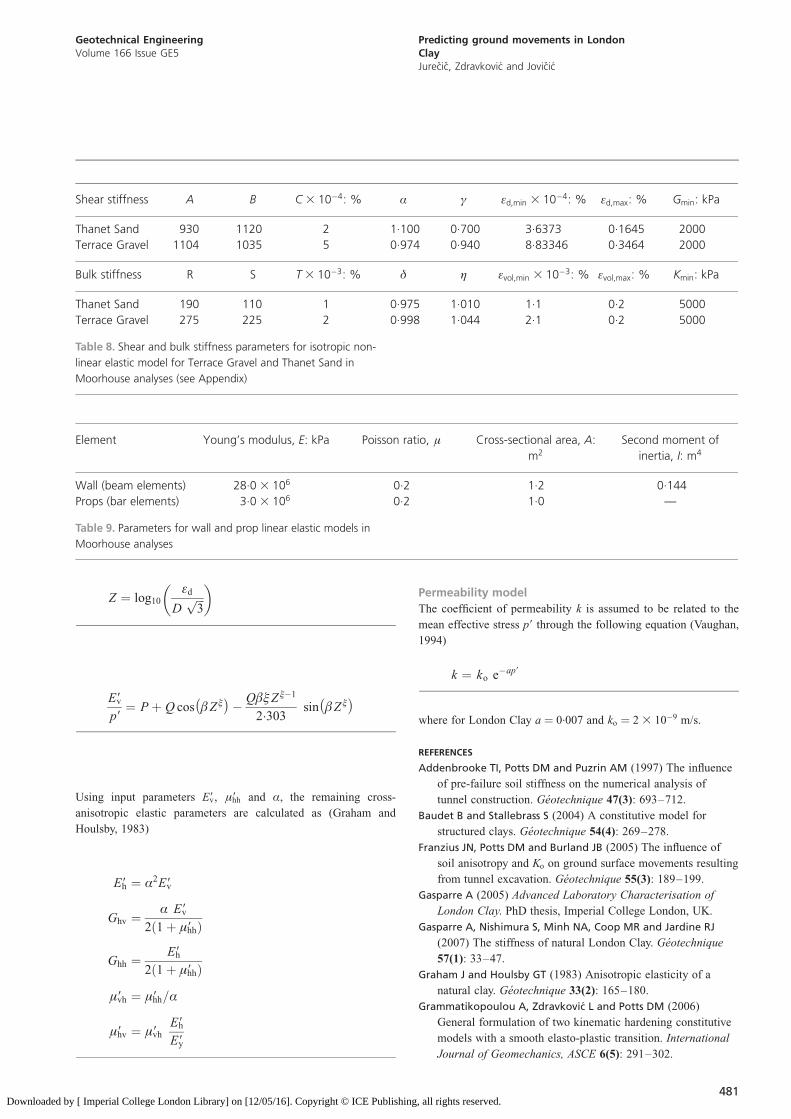
Shear stiffness A B C 3 10�4: % Æ ª �d,min 3 10�4: % �d,max: % Gmin: kPa
Thanet Sand 930 1120 2 1.100 0.700 3.6373 0.1645 2000
Terrace Gravel 1104 1035 5 0.974 0.940 8.83346 0.3464 2000
Bulk stiffness R S T 3 10�3: % � � �vol,min 3 10�3: % �vol,max: % Kmin: kPa
Thanet Sand 190 110 1 0.975 1.010 1.1 0.2 5000
Terrace Gravel 275 225 2 0.998 1.044 2.1 0.2 5000
Table 8. Shear and bulk stiffness parameters for isotropic non-
linear elastic model for Terrace Gravel and Thanet Sand in
Moorhouse analyses (see Appendix)
Element Young’s modulus, E: kPa Poisson ratio, � Cross-sectional area, A:
m2
Second moment of
inertia, I: m4
Wall (beam elements) 28.0 3 106 0.2 1.2 0.144
Props (bar elements) 3.0 3 106 0.2 1.0 —
Table 9. Parameters for wall and prop linear elastic models in
Moorhouse analyses
481
Geotechnical EngineeringVolume 166 Issue GE5
Predicting ground movements in LondonClayJurecic, Zdravkovic and Jovicic
Downloaded by [ Imperial College London Library] on [12/05/16]. Copyright © ICE Publishing, all rights reserved.
Grammatikopoulou A, St John HD and Potts DM (2008) Non-
linear and linear models in design of retaining walls.
Proceedings of the Institution of Civil Engineers –
Geotechnical Engineering 161(6): 311–323.
Higgins KG, Potts DM and Mair RJ (1996) Numerical modelling
of the influence of the Westminster Station excavation and
tunnelling on Big Ben clock tower. In Proceedings of the
International Symposium on Geotechnical Aspects of
Underground Construction in Soft Ground, London, UK
(Mair RJ and Taylor RN (eds)). Balkema, Rotterdam, the
Netherlands, pp. 525–530.
Hight DW and Higgins KG (1994) An approach to the prediction
of ground movements in engineering practice: background
and application. In Proceedings of the International
Symposium on Pre-failure Deformation of Geomaterials,
Hokkaido, Japan (Shibuya S, Mitachi T and Miura S (eds)).
Balkema, Rotterdam, the Netherlands, pp. 909–945.
Hight DW, Gasparre A, Nishimura S et al. (2007) Characteristics
of the London Clay from the Terminal 5 site at Heathrow
Airport. Geotechnique 57(1): 3–18.
Jardine RJ, Potts DM, Fourie AB and Burland JB (1986) Studies
of the influence of non-linear stress–strain characteristics in
soil–structure interaction. Geotechnique 36(3): 377–396.
Kanapathipillai A (1996) Review of the BRICK Model of Soil
Behaviour. MSc thesis, Imperial College, London, UK.
Kavvadas M and Amorosi A (2000) A constitutive model for
structured soils. Geotechnique 50(3): 263–273.
Lambe TW (1973) Predictions in soil engineering. Geotechnique
23(2): 149–202.
Mair RJ (2008) Tunnelling and geotechnics: new horizons.
Geotechnique 58(9): 695–736.
Manzari MT and Dafalias YF (1997) A critical state two-surface
plasticity model for sands. Geotechnique 47(2): 255–272.
Potts DM and Zdravkovic L (1999) Finite Element Analysis in
Geotechnical Engineering: Theory. Thomas Telford, London,
UK.
Potts DM and Zdravkovic L (2001) Finite Element Analysis in
Geotechnical Engineering: Application. Thomas Telford,
London, UK.
Schroeder FC, Higgins KG, Wright P and Potts DM (2011)
Assessment of overbridge openings on the London
Underground tunnel network. Proceedings of the 15th
European Conference on Soil Mechanics and Geotechnical
Engineering– XV ECSMGE, Athens, Greece, pp. 1733–1738.
Simpson B (1992) Retaining structures: displacement and design.
Geotechnique 42(4): 541–576.
Simpson B, O’Riordan NJ and Croft DD (1979) A computer
model for the analysis of ground movements in London Clay.
Geotechnique 29(2): 149–175.
Simpson B, Atkinson JH and Jovicic V (1996) The influence of
anisotropy on calculations of ground settlements above
tunnels. In Proceedings of the International Symposium on
Geotechnical Aspects of Underground Construction in Soft
Ground, London, UK (Mair RJ and Taylor RN (eds)).
Balkema, Rotterdam, the Netherlands, pp. 591–594.
Stallebrass SE, Jovicic V and Taylor RN (1994) Short term and long
term settlements around a tunnel in stiff clay. In Proceedings
of the 3rd European Conference on Numerical Methods in
Geotechnical Engineering, Manchester, UK (Smith IM (ed.)).
Balkema, Rotterdam, the Netherlands, pp. 235–240.
Standing JR, Nyren RJ, Burland JB and Longworth TI (1996) The
measurement of ground movement due to tunnelling at two
control sites along the Jubilee Line Extension. In Proceedings
of the International Symposium on Geotechnical Aspects of
Underground Construction in Soft Ground, London, UK
(Mair RJ and Taylor RN (eds)). Balkema, Rotterdam, the
Netherlands, pp. 751–756.
Vaughan PR (1994) Assumption, prediction and reality in
geotechnical engineering. Geotechnique 44(4): 573–603.
Zdravkovic L, Potts DM and St John HD (2005) Modelling of a
3D excavation in finite element analysis. Geotechnique 55(7):
497–513.
WHAT DO YOU THINK?
To discuss this paper, please email up to 500 words to the
editor at [email protected]. Your contribution will be
forwarded to the author(s) for a reply and, if considered
appropriate by the editorial panel, will be published as a
discussion in a future issue of the journal.
Proceedings journals rely entirely on contributions sent in
by civil engineering professionals, academics and students.
Papers should be 2000–5000 words long (briefing papers
should be 1000–2000 words long), with adequate illustra-
tions and references. You can submit your paper online via
www.icevirtuallibrary.com/content/journals, where you
will also find detailed author guidelines.
482
Geotechnical EngineeringVolume 166 Issue GE5
Predicting ground movements in LondonClayJurecic, Zdravkovic and Jovicic
Downloaded by [ Imperial College London Library] on [12/05/16]. Copyright © ICE Publishing, all rights reserved.