Predicting geological features in 3D Seismic Data

Taylor Dahlke, Mauricio Araya-PoloShell Int. E&P Inc.

Chiyuan Zhang, Charlie Frogner, Tomaso PoggioMassachusetts Institute of Technology

Abstract

We present a novel approach to a challenging 3D imaging problem, using deeplearning to map out a network of faults in the earth’s subsurface, directly fromseismic recordings. We exploit fault continuity through a novel loss function, theWasserstein loss, and demonstrate high accuracy predictions on synthetic models.

1 Introduction

Seismic imaging is an essential tool in oil and gas (O&G) exploration. In seismic imaging, one hopesto image the subsurface rock layers and other geological features, using measurements typicallycomprising reflected sound waves recorded by a microphone array at the surface. Reconstructinga seismic image is a difficult inverse problem, requiring initialization from prior knowledge andextensive manual intervention by domain experts, in a process that can take months to complete.

Impermeable

Shale clay

Porous

Reservoir rock

Source rock

Oil well

Natural gas

Rock oil

Fault

Figure 1: Left: Fault in relation to a hydrocarbon system. Center: fault structure in an outcrop. Right:visualization of conical fault surfaces after the inverse problem has been solved[3].

The key geological feature we target here is a fault network, which is a network of fractures alongwhich there is significant displacement of the abutting rock (Fig. 1.center). Faults are of significantinterest in seismology, as they can be the site of earthquake activity. Furthermore, in O&G explo-ration the shifting rock layers can trap liquid hydrocarbons which will form reservoirs (Fig. 1.left).Importantly, the 3D structure of a fault network can be quite complex (Fig. 1.right), representing achallenge for structured output methods.

In this work, we propose a machine learning approach to address a subproblem within seismicimaging. Particularly, we propose to use the raw seismic measurements that are inputs to the seismicimaging process, to map out important geological features that would normally be the outcome ofexpert analysis of the final seismic image. In other words, we bypass the seismic imaging processentirely, while producing a map of key features of interest. Traditional computer vision basedalgorithms do not apply here, because the spatial correspondence between the raw time-series signalsand the seismic images is unknown.

3D Deep Learning Workshop at NIPS 2016, Barcelona, Spain.

2 Synthesizing Geological Data and Related Work

The seismic imaging problem, as do many physical inverse problems, offers a distinct advantagein that we can simulate training data, as the measurement process which generates the raw data forseismic imaging is well-understood physically. This property is shared by seismic imaging and anumber of physical inverse problems in oceanography and the atmospheric and climate sciences. Forthe case of seismic imaging, the measurement process maps a given subsurface geology to a set ofseismological measurements (Fig. 2.top-center), and we are able to simulate these measurementsgiven any subsurface model. As a result, we can train our machine learning model using syntheticdata. This is important because collecting and especially labeling the real data is a very expensiveprocess.

We exploit the well-understood forward problem, which models wave propagation beneath the earthsurface, to synthesize training data for our machine learning algorithm. Let v be a random variablerepresenting the velocity model, which captures the main underground layer structure. A generativemodel for our problem is x← v→ y, where x is the corresponding seismic traces, and y is labelingoutput, representing locations of faults.

We build a custom model synthesizer that generates random, geologically-feasible velocity models(Fig. 2.top-left). The corresponding seismic traces are obtained by solving a finite differenceapproximation to the acoustic wave equations. We avoid full probabilistic inference (e.g. viaEM), because computing the latent variable v entails solving the full inverse problem. We instead usethe generated data to learn a deep neural network model for p(y|x). This is a structured predictionproblem, characterized both by the geometrical nature of the output (being complex networks of 3Dsurfaces) and by the potential scale (with 3D datasets running into the billions of voxels).

In a previous work [5], a single planar fault in the 2D world is represented by a location and angleof descent. Moving to more realistic data which can contain multiple faults systems, we encodethe output in a grid of binary values each indicating the presence or absence of a fault in a grid cell.This representation also naturally generalize to 3D cases. Most other related work on automaticallydetecting geological features (e.g. [2]) are based on migrated seismic images, instead of the originalreflection waveforms as what we do in this paper.

3 Structured Output Learning and the Wasserstein Loss

Our problem is naturally formulated as predicting a (subsampled) 3D “pixel map” of binary fault/ non-fault indicators. This is similar to the image segmentation problems in computer vision. Acommon way of handling this is to introduce a Markov Random Field (MRF) on the output variablesthat captures the couplings and run an inference algorithm to get the jointly optimal predictions. Moregenerally, the inference step can be incorporated into the objective function for learning. Commonlyused formulations include structured SVM and Conditional Random Fields [4].

However, while the couplings for pixel labels in an image can be naturally modeled via neighborhoodsimilarity or input-pixel based similarity, the prior structure in our model is of much higher order.More specifically, the faults usually extend as smooth surfaces. This property cannot be characterizedvia factors that involves only a few nearby output variables. On the other hand, inference on MRFswith general high order factors is computationally expensive. As a result, we choose to performindependent prediction for each output region, and incorporate our prior via a novel loss functioncalled the Wasserstein Loss [1].

Formally, let K = D ×D ×D be the number of output cells. We normalize the ground-truth binaryoutput vector y ∈ {0, 1}K to y = y/‖y‖1 so that it represents a probability distribution over the 3Dgrid. Moreover, we model our predictor as a deep neural network with a softmax layer at the top, sothat it also produce a probability distribution hθ(x) ∈ ∆K , where ∆K is the K-dimensional simplex,and θ is all the parameters in the deep neural network.

The cross-entropy loss is commonly used to measure the difference between two distributions. Itis derived from the KL-divergence between the prediction y and the ground-truth y: `CE(y, y) =∑Kk=1 yk log yk, for y, y ∈ ∆K . When the ground-truth y is an encoded vector for a single class, this

reduces to the cross-entropy loss typically used in multiclass logistic regression. This loss, however,does not consider the structural information for the fault prediction problems. Specifically, the spatial

2

SeismicTracesfromWave

Equation

Physics

Labels

Deep Learning Model Inputs

Fault Predictions

Figure 2: Left: the workflow of our deep learning based fault prediction system. Right: 2D illustrationof the cross-entropy loss vs. the Wasserstein loss. The red cells are ground truth, and the blue cellsare predictions. The cross-entropy loss treats both predictions equally while the Wasserstein lossfavors the bottom figure for the spatial smoothness.

relationship among the K output cells could enforce strong smoothness information. Consider aprediction that is slightly off the ground truth, and another one that is completely wrong, as shown inFigure 2; the cross entropy loss cannot effectively distinguish the two different cases.

Alternatively, consider the following Wasserstein loss [1],

`W (y, y) = minT∈Π(y,y)

〈T,M〉, Π(y, y) = {T ∈ RK×K+ : T1 = y, T>1 = y} (1)

where 〈T,M〉 = tr(T>M) is the inner-product, for a given ground metric matrix Mk,k′ = d(k, k′)for some ground metric d(·, ·) on the output space. For our application, the output space is the 3Dgrid of cells, and the natural metric is the Euclidean distance between the cells.

T in the loss term is a joint probability distribution that marginalize to the ground-truth and theprediction. Intuitively, T defines a transportation plan that maps probability mass from the predictionto the ground-truth, and 〈T,M〉 measures the cost of this plan according to the ground metric. Theloss is then defined by the cost of the optimal feasible transportation plan. For the cases of Figure 2,the Wasserstein loss for the bottom right figure will be smaller than the top right figure, due to thelonger the cost of this plan according to the ground metric. The loss is defined by the cost of theoptimal plan.

4 Results

We evaluated the performance of our deep learning approach on a set of synthetic, randomly generatedgeophysical models and corresponding simulated measurements. The geophysical models had severalsubsurface layers with varying rock properties, and either one or two major planar faults at randomorientations and locations. Seismic recordings were simulated for each model for a regularly spacedarray of 20 × 20 surface microphones, with 9 initial shots or impulses at evenly spaced surfacelocations, using an acoustic approximation to the wave equation.

We trained a variety of fully-connected deep neural networks with 4 to 6 hidden layers of varyingnumbers of units. The output of the networks was a 20× 20× 20 3D voxel grid, with each voxel’svalue indicating the likelihood of a fault being present within the voxel. Ground truth labels on thesame grid were binary-valued, indicating presence or not of a fault in each voxel. In all cases, weused a Wasserstein loss function for training.

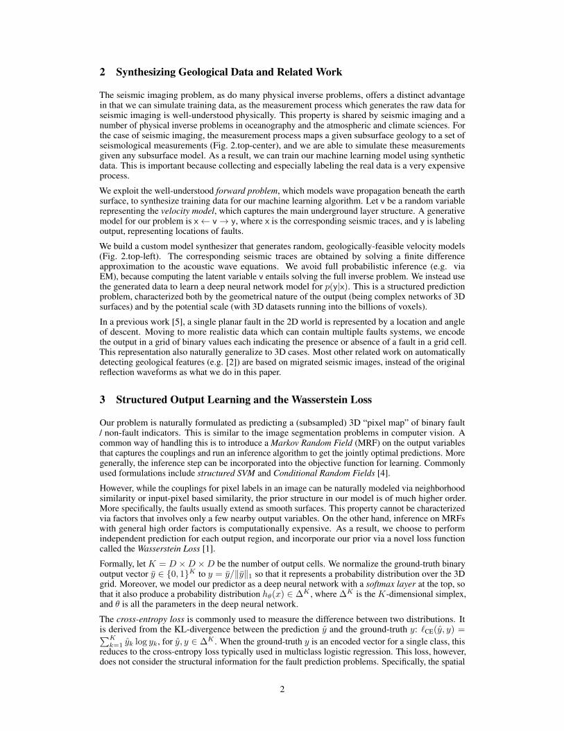
Table 1 shows the best results obtained, on several sets of simulated test data. We report the areaunder the ROC curve (AUC) for the predictions, comparing predicted likelihoods for the voxelscontaining a ground truth labeled fault to those not containing a fault. We also report the intersectionover union (IoU) value, averaged over the test set images, with predicted likelihoods thresholded at avalue chosen to maximize the average IoU over the images. For datasets with one and two planar

3

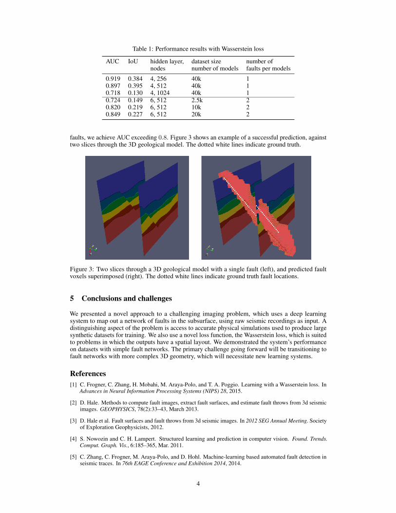
Table 1: Performance results with Wasserstein loss

AUC IoU hidden layer, dataset size number ofnodes number of models faults per models

0.919 0.384 4, 256 40k 10.897 0.395 4, 512 40k 10.718 0.130 4, 1024 40k 10.724 0.149 6, 512 2.5k 20.820 0.219 6, 512 10k 20.849 0.227 6, 512 20k 2

faults, we achieve AUC exceeding 0.8. Figure 3 shows an example of a successful prediction, againsttwo slices through the 3D geological model. The dotted white lines indicate ground truth.

Figure 3: Two slices through a 3D geological model with a single fault (left), and predicted faultvoxels superimposed (right). The dotted white lines indicate ground truth fault locations.

5 Conclusions and challenges

We presented a novel approach to a challenging imaging problem, which uses a deep learningsystem to map out a network of faults in the subsurface, using raw seismic recordings as input. Adistinguishing aspect of the problem is access to accurate physical simulations used to produce largesynthetic datasets for training. We also use a novel loss function, the Wasserstein loss, which is suitedto problems in which the outputs have a spatial layout. We demonstrated the system’s performanceon datasets with simple fault networks. The primary challenge going forward will be transitioning tofault networks with more complex 3D geometry, which will necessitate new learning systems.

References[1] C. Frogner, C. Zhang, H. Mobahi, M. Araya-Polo, and T. A. Poggio. Learning with a Wasserstein loss. In

Advances in Neural Information Processing Systems (NIPS) 28, 2015.

[2] D. Hale. Methods to compute fault images, extract fault surfaces, and estimate fault throws from 3d seismicimages. GEOPHYSICS, 78(2):33–43, March 2013.

[3] D. Hale et al. Fault surfaces and fault throws from 3d seismic images. In 2012 SEG Annual Meeting. Societyof Exploration Geophysicists, 2012.

[4] S. Nowozin and C. H. Lampert. Structured learning and prediction in computer vision. Found. Trends.Comput. Graph. Vis., 6:185–365, Mar. 2011.

[5] C. Zhang, C. Frogner, M. Araya-Polo, and D. Hohl. Machine-learning based automated fault detection inseismic traces. In 76th EAGE Conference and Exhibition 2014, 2014.

4