ISSN: 1439-2305

Number 326 – November 2017

PREDICTING EXCHANGE RATES IN

ASIA: NEW INSIGHTS ON THE

ACCURACY OF SURVEY FORECASTS

Frederik Kunze

Predicting exchange rates in Asia:

New insights on the accuracy of survey forecasts

Frederik Kunze∗†‡

Abstract

This paper evaluates aggregated survey forecasts with forecast horizons of 3, 12,and 24 months for the exchange rates of the Chinese yuan, the Hong Kong dollar,the Japanese yen, and the Singapore dollar vis-à-vis the US dollar using commonforecast accuracy measures. Additionally, the rationality of the exchange rate pre-dictions are assessed utilizing tests for unbiasedness and efficiency. All investigatedforecasts are irrational in the sense that the predictions are biased. However, theseresults are inconsistent with an alternative measure of rationality based on methodsof applied time series analysis. Investigating the order of integration of the timeseries and using cointegration analysis, empirical evidence supports the conclusionthat the majority of forecasts are rational. Regarding forerunning properties ofthe predictions, the results are less convincing, with shorter term forecasts for thetightly managed USD/CNY FX regime being one exception. As one importantevaluation result, it can be concluded, that the currency regime matters for thequality of exchange rate forecasts.

JEL classification: F31, F37, G17, O24.

Keywords: Exchange rates, survey forecasts, forecast evaluation, forecast acccuracy, fore-cast rationality, cointegration, impulse response analysis.

∗Corresponding author: E-Mail frederik.kunze@nordlb.de, phone +49 511 361 5380†Georg-August-University, Göttingen, Germany‡NORD/LB Norddeutsche Landesbank Girozentrale, Hannover, Germany

1. Introduction

The foreign exchange (FX) market belongs to the largest financial markets globally

(see, for example, Sosvilla-Rivero and Ramos-Herrera, 2013). Additionally, exchange

rates are crucial price variables in open economies and international finance (see Dreger

and Stadtmann, 2008; Dick, MacDonald, and Menkhoff, 2015) and have a significant

impact on foreign trade and cross border investments (see, for example, Kan, 2017).

Hence, the understanding of the price building processes in the FX market is relevant

for decision makers in general and for forecasters in particular (Ince and Molodtsova,

2017). This is also true for Asian currencies, because with respect to global GDP growth,

cross border investments and world trade Asian economies are becoming increasingly

important, and, in recent years, asset managers outside Asia seeking to diversify their

investment positions are focusing on Asia’s financial markets (see, for example, Dunis

and Shannon, 2005).

During the global financial crisis, various currencies have been under pressure of a

pronounced and unanticipated appreciation of the US dollar (Fratzscher, 2009). These

movements are a potential source of severe economic and financial consequences, be-

cause uncertainty regarding exchange rate movements might hinder economic activity

including cross border trade (see, for example, Thorbecke, 2008; Chit, Rizov, and Wil-

lenbockel, 2010). Hayakawa and Kimura (2009) have shown that especially in East Asia

intra-regional trade is negatively affected by FX volatility. In addition to that, both

foreign and domestic companies have to deal with currency risk (see Aggarwal, Chen,

and Yur-Austin, 2011; Aggarwal, 2013). De Grauwe and Markiewicz (2013) note that

especially in non-U.S. equity markets, and in certain sub-periods, currency risks have

been the major driver of risk premiums in the stock market. Since currency risk is non-

neglectable, FX forecasts may create economic value for financial market participants,

central banks, policy decision makers as well as importers and exporters. Following Duffy

and Giddy (1975), FX forecasts have to be seen as “significant inputs to decisions con-

cerning practically every aspect of international business” (see Duffy and Giddy, 1975, p.

1).

Owing to the growing importance of Asia’s major economies and the region’s most

important financial centers, this paper focuses on the investigation of forecasts for ex-

change rates of the Chinese yuan, the Hong Kong dollar, the Japanese yen, and the

Singapore dollar vis-à-vis the US dollar. Using measures of forecast accuracy, common

tests for rationality (i.e. unbiasedness and efficiency), as well methods of applied time

series analysis (i.e. cointegration analysis and impulse response functions), the quality

of survey forecasts for these exchange rates will be assessed. As a consequence of signif-

icant differences in FX regimes in the currency areas under investigation, it will also be

examined whether there exists empirical evidence for regime dependent variations in the

1

quality of survey forecasts.

Given the relevance of the FX regime on the price building processes for exchange

rates, it is expected that survey forecasts do vary regarding accuracy and rationality. For

forecasters classifying the relevant exchange rate regime is a crucial step (see, for example,

Von Spreckelsen, Kunze, Windels, and von Mettenheim, 2014). Against the background

of a strong influence of policy makers on exchange rates in managed FX regimes and the

statutory provisions in currency boards it is standing to reason, that fixed and strongly

managed exchange rates are “easier” to forecast, because policy makers are following an

anticipated or even mandatory agenda. On the other hand, free float FX regimes seem

to lack these policy guidelines which makes it more difficult to forecast the future path

of exchange rates. Hence, while focusing on the investigation of survey based exchange

rate forecasts provided by Consensus Economics for four different currency regimes, this

paper seeks to combine two strands of research dealing with FX forecast evaluation and

FX regimes and, while doing so, to fill a relevant gap in the literature.

The remainder of the paper is structured as follows. Chapter 2 delivers an overview of

the relevant literature. Chapter 3 lists the chosen currency areas as well as the data set

and describes the underlying regimes. Before exhibiting the methodological framework

Chapter 4 delivers initital empirical results. Chapter 5 presents the evaluation results.

Chapter 6 discusses the implications of the results in more detail and concludes the paper.

2. Literature overview

Frenkel and Mussa (1980) note that policy makers have to deal with FX market

fluctuations and that the predictability of FX rates is important in this context. Never-

theless, they also comment that “the facts indicate, however, that exchange-rate changes

are largely unpredictable” (see Frenkel and Mussa, 1980, p. 374). In their seminal pa-

per Meese and Rogoff (1983) discuss the inability of fundamental models to forecast

exchange rates in detail and motivate a large body of research dealing with the quality

of FX predictions (see, for example, Frankel and Rose, 1994; Cheung and Chinn, 1998;

Kilian and Taylor, 2003; Frenkel, Mauch, Rülke, et al., 2017, to name but a few). De-

spite the findings of Meese and Rogoff (1983) as well as Frenkel and Mussa (1980), FX

survey forecasts are still of relevance for economic agents. Especially for financial market

practitioners and decision makers, unable or unwilling to build up forecasting models for

numerous financial variables of their own, survey forecasts (for exchange rates) may serve

as one alternative. Ter Ellen, Verschoor, and Zwinkels (2013) annotate that investors in

the FX market have to gather costly information to be able to form expectations. Not

surprisingly, FX survey forecasts (both in aggregated and disaggregated form) have been

intensively assessed with regard to their rationality (as regards, for example, unbiasedness

2

and efficiency) as well as accuracy.

In the context of the evaluation of FX survey forecasts, data sets from numerous

providers have been used.1 Especially, the rationality of FX predictions, which is also in

the focus of this paper, has been analyzed intensively (see, for example, Audretsch and

Stadtmann, 2005; De Grauwe and Markiewicz, 2013; Rülke and Pierdzioch, 2013) with

diverging results. Audretsch and Stadtmann (2005), who focus on disaggregated survey

forecasts from the Wall Street Journal, find no evidence for the assumption of rational

agents forming homogeneous expectations. Dominguez (1986) investigates survey fore-

casts for FX markets in emerging economies and concludes that the rational expectation

hypothesis has to be rejected. Avraham, Ungar, and Zilberfarb (1987) find similar ev-

idence for the Israeli shekel. Frenkel, Mauch, Rülke, et al. (2017) examine forecasters’

rationality regarding exchange rate predictions. Their work is of high relevance for the

focus of this paper because the authors empirically assess differences between currency

forecasts for developed and emerging economies. They present a link between forecast

accuracy as well as rationality and different currency areas and, hence, fill a relevant gap

in the literature on FX survey forecast evaluation.

Focusing on a specific Asian market, Tsuchiya and Suehara (2015) investigate forecasts

provided by Consensus Economics for the USD/CNY exchange rates between July 2005

and December 2012. The authors examine the directional accuracy of the forecasts and

conclude that forecasters are not inferior to a naïve benchmark. Tsuchiya and Suehara

(2015) find evidence for changes in FX forecasters herding behavior due to the financial

crisis and central bank interventions and conclude that the monetary policy respectively

the currency regime is of high relevance when evaluating FX forecasts. Duffy and Giddy

(1975) compare the predictability of flexible and fixed exchange regimes and state that

predictions for flexible exchange rates are futile. The monetary authorities’ influence on

the Japanese FX market (i.e. the exchange rate between the Japanese yen and the US

dollar) and the resulting forecast dispersion has been assessed by Reitz, Stadtmann, and

Taylor (2010). Also using data provided by Consensus Economics the authors conclude

that while with increasing volatility of the USD/JPY FX forecast dispersion increases,

policy interventions in the FX market have dampening effects on forecast dispersion.

MacDonald and Nagayasu (2015) evaluate USD/JPY forecasts provided by the Japan

1In addition to the forecasts provided by Consensus Economics (Leitner and Schmidt, 2006;Beine, Bénassy-Quéré, and MacDonald, 2007; Jongen, Verschoor, Wolff, and Zwinkels, 2012; Ince andMolodtsova, 2017) predictions collected via the Wall Street Journal (WSJ) Poll (Audretsch and Stadt-mann, 2005; Mitchell and Pearce, 2007; Frenkel, Rülke, and Stadtmann, 2009; Rülke, Frenkel, andStadtmann, 2010), FX Week (e.g. Ter Ellen et al., 2013), Bloomberg (e.g. Pancotto, Pericoli, and Pistag-nesi, 2014), Forecasts Unlimited (Bacchetta, Mertens, and Van Wincoop, 2009; Beckmann and Czudaj,2017a,b; Ince and Molodtsova, 2017), Blue Chip Forecasts (Baghestani, 2010), Reuters (e.g. Bofingerand Schmidt, 2003) as well as the ZEW Finanzmarkttest (e.g. Bofinger and Schmidt, 2003; Leitner andSchmidt, 2006; Spiwoks and Hein, 2007; Heiden, Klein, and Zwergel, 2013) have been investigated. Thedata sets provided from Consensus Economics which come to use in this paper carry the advantages ofa large historical database and three forecast horizons.

3

Center for International Finance (JCIF) survey and conclude that predictions are irra-

tional.

When examining Asia’s foreign exchange markets it has to be acknowledged that,

unlike in the EMU, there does not exist a common currency area in Asia. Even more

than that, currency regimes do vary significantly. Following, for example, Klein and

Shambaugh (2008) it can be stated that the choice of the FX regime does matter and

is a central topic in international finance. For a lot of currency areas, the bipolar seg-

mentation between hard pegs or free floating only appears on the surface (Obstfeld and

Rogoff, 1995; Calvo and Reinhart, 2002). For example, Moosa and Li (2017) remark

that in the case of China the identification of the FX regime is important for the de-

bate whether the Chinese currency is undervalued or not. This, in turn, is a relevant

decision variable for forecasters. Having said that, it has to be taken into consideration

that with the course of time monetary respectively FX regimes have changed manifold

(Hernandez and Montiel, 2003; Bordo, Choudhri, Fazio, and MacDonald, 2017). More-

over, most emerging economies do not have a long track record when it comes to floating

FX regimes (Kohlscheen, 2014). As a matter of fact, professional forecasters might also

adjust their behavior when publishing forecasts for different FX regimes. Chinn and

Frankel (1994) note that forecasters might be reluctant to deliver naïve predictions –

especially for unstable currencies. Duffy and Giddy (1975), focusing on flexible exchange

rates, present results indicating that for major exchange rates forecasting is not profitable.

3. Data set and FX regime classification

The monthly mean of survey FX forecasts with regard to four Asian currencies col-

lected by Consensus Economics is used. The data set contains three different forecast

horizons (3, 12, and 24 months) and ranges from January 1999 to March 2017. Forecasts

for the following exchange rates will be evaluated: Chinese yuan against the US dollar

(USD/CNY), Hong Kong dollar against the US dollar (USD/HKD), Japanese yen against

the US dollar (USD/JPY), and Singapore dollar against US dollar (USD/SGD).2

The four exchange rates are suitable for the purpose of this paper for various reasons.

Firstly, the currency areas are of high economic relevance in Asia and / or fulfill an im-

portant role in global financial markets. In terms of nominal GDP, for example, China

respectively Japan are the two largest economies in Asia and number two respectively

three globally. Furthermore, China is the world’s largest trade nation (as measured by

exports plus imports) and the Japanese currency plays an important role as a safe haven

2Throughout the paper all exchange rates are given as units per US dollar. Hence, a rise in theexchange rate corresponds to a US dollar appreciation and a lower exchange rate corresponds to adepreciation of the US dollar.

4

asset for investors. Hong Kong and Singapore as city states share the common character-

istic to belong to the world’s most sophisticated financial centers (see, for example, Tse

and Yip, 2006; Woo, 2016). Secondly, the four currency areas do vary significantly when

it comes to their FX regimes (see, for example, Tse and Yip, 2006; Cheung, Chinn, and

Fujii, 2007; Chow, 2007; Takagi, 2007). Since this study also aims to examine possible

differences in the forecast accuracy controlling for the FX regime this classification is

important for the purpose of this paper.

However, the officially announced de jure exchange rate regimes do very often deviate

from the observable de facto exchange rate regimes (see Obstfeld and Rogoff, 1995; Calvo

and Reinhart, 2002; Klein and Shambaugh, 2008; Patnaik, Shah, Sethy, and Balasub-

ramaniam, 2011). Additionally, currency regimes are not necessarily stable over time.

Since 1998, the IMF publishes de facto classifications of the countries’ FX regimes (see

Kokenyne, Veyrune, Habermeier, and Anderson, 2009). To ensure comparability the FX

regime classification in this paper is taken from the official IMF publication Annual Report

on Exchange Arrangements and Exchange Restrictions (i.e. years 2000 to 2016). This de

facto classification is useful because it is regularly updated (Patnaik, Shah, Sethy, and

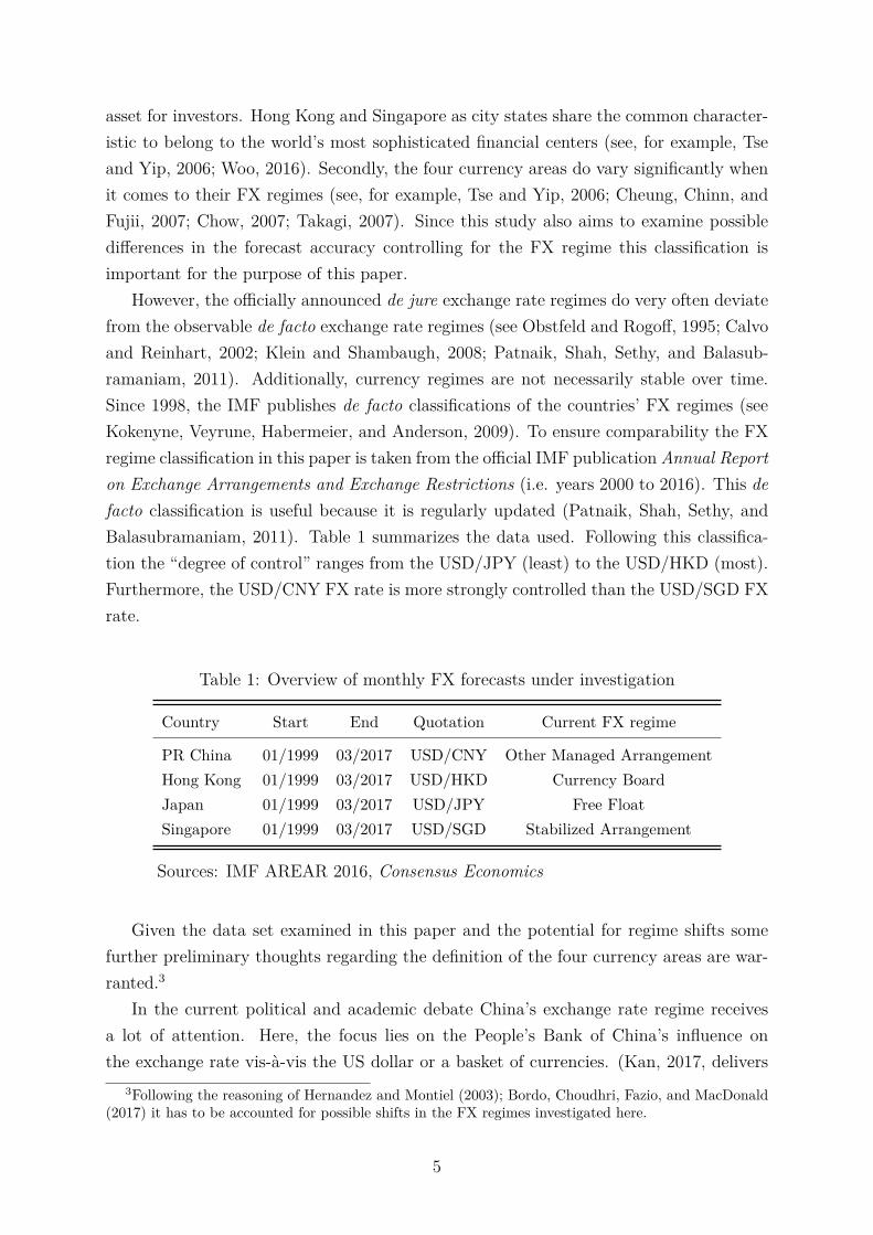
Balasubramaniam, 2011). Table 1 summarizes the data used. Following this classifica-

tion the “degree of control” ranges from the USD/JPY (least) to the USD/HKD (most).

Furthermore, the USD/CNY FX rate is more strongly controlled than the USD/SGD FX

rate.

Table 1: Overview of monthly FX forecasts under investigation

Country Start End Quotation Current FX regime

PR China 01/1999 03/2017 USD/CNY Other Managed Arrangement

Hong Kong 01/1999 03/2017 USD/HKD Currency Board

Japan 01/1999 03/2017 USD/JPY Free Float

Singapore 01/1999 03/2017 USD/SGD Stabilized Arrangement

Sources: IMF AREAR 2016, Consensus Economics

Given the data set examined in this paper and the potential for regime shifts some

further preliminary thoughts regarding the definition of the four currency areas are war-

ranted.3

In the current political and academic debate China’s exchange rate regime receives

a lot of attention. Here, the focus lies on the People’s Bank of China’s influence on

the exchange rate vis-à-vis the US dollar or a basket of currencies. (Kan, 2017, delivers

3Following the reasoning of Hernandez and Montiel (2003); Bordo, Choudhri, Fazio, and MacDonald(2017) it has to be accounted for possible shifts in the FX regimes investigated here.

5

a good summary of the discussion). In recent years, the Chinese authorities carried

out far reaching adjustments to the FX regime (Cheung, Hui, and Tsang, 2016, 2017).

Most importantly, in 2005, the central bank announced that the Chinese currency would

switch to a managed float regime “with reference to a basket of currencies” (see Tian

and Chen, 2013, p. 16). Moosa and Li (2017) deliver a clear overview of the 2005

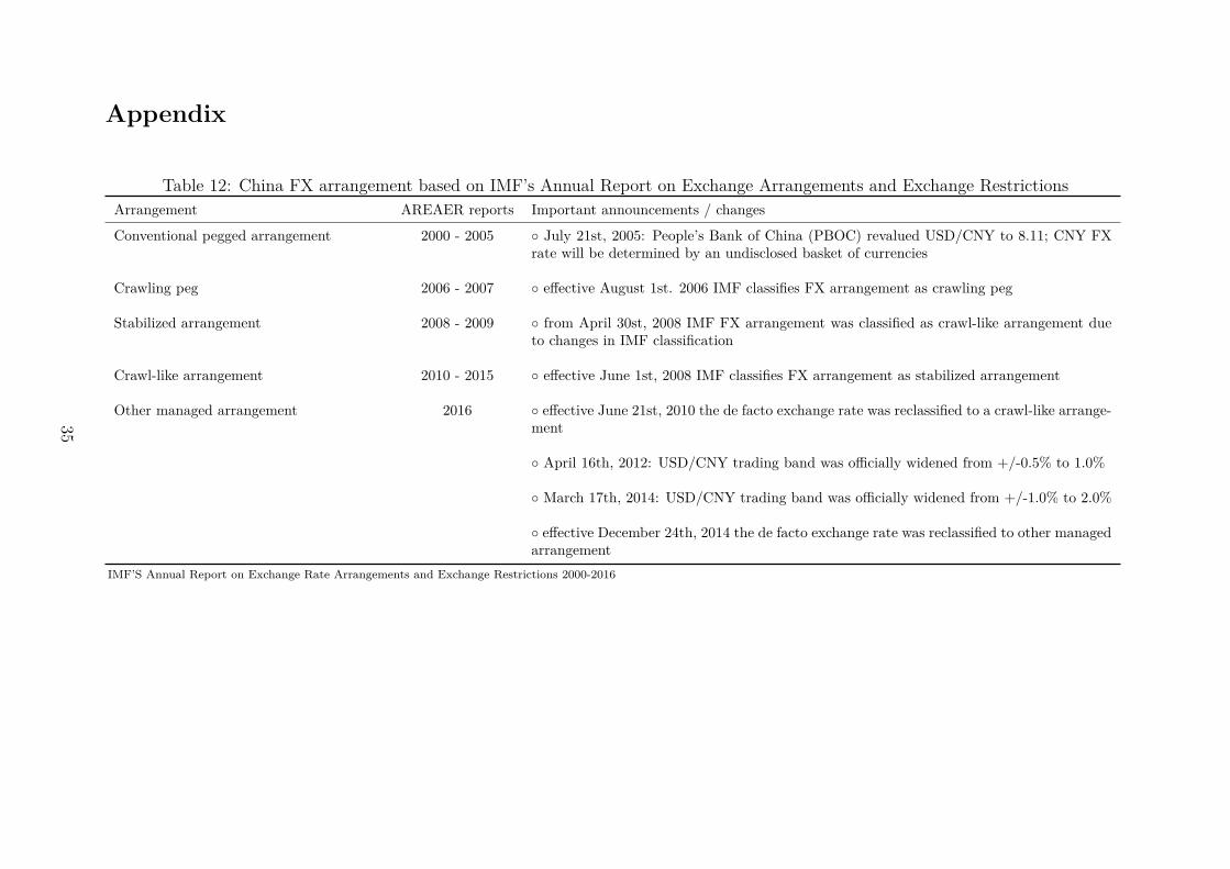
adjustments and the subsequent steps. The IMF’s de facto classification, as well as

important announcements by the Chinese government, can be found in Table 12 in the

Appendix.4

In contrast to the Chinese FX regime the Japanese currency’s floating exchange rate

regime is already in place since 1973 (see, for example, Hamada and Hayashi, 1985;

Hutchison and Walsh, 1992, as well as Table 15 in the Appendix). Hence, the existence

of regime shifts with relevance for the focus of this paper can be ruled out completely. The

same holds true for the currency board system of Hong Kong, which has been established

as early as 1983 and, since, has been in place (see, for example, Ho, 2002; Cook and

Yetman, 2014, as well as Table 13 in the Appendix). In contrast, the Monetary Authority

of Singapore (MAS) operates an exchange rate based monetary policy and, hence, the

FX rate is practically the instrument to steer both output and inflation (see, for example,

Siregar, Har, et al., 2001; Devereux, 2003; Chow, 2007; Chow, Lim, and McNelis, 2014, as

well as Table 15 in the Appendix). As a consequence there does not exist a free floating

USD/SGD exchange rate, but a managed regime which occasionally results in the more

volatile exchange rate vis-à-vis the US dollar in comparison to the Hong Kong dollar

(Devereux, 2003).5 This regime lasts for the entire time period under investigation.

4. Initial empirical analysis and methodological frame-

work

Before starting to evaluate the forecasts for the FX rates it is necessary to investigate

the trending behavior of the exchange rate time series and the corresponding forecasts.

To test for unit roots, the non-parametric test procedure proposed by Phillips and Perron

(1988) will be used. The results of the PP (Phillips and Perron) unit root tests in levels

and first differences (∆) are given in Table 2 below.

4The regime change in 2005 might also be relevant for the focus of this paper. Because of that,robustness checks will be executed. It is important to note that for the USD/CNY FX rate controllingfor the notable regime shift in July 2005 would lead to a shorter data period ranging from August 2005to March 2017.

5Based on standard deviation of log differences as an approximation of returns the volatility is highestfor the USD/JPY, followed by the USD/SGD, USD/CNY, and USD/HKD.

6

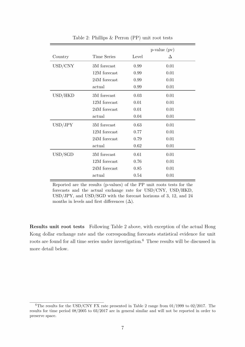
Table 2: Phillips & Perron (PP) unit root tests

p-value (pv)

Country Time Series Level ∆

USD/CNY 3M forecast 0.99 0.01

12M forecast 0.99 0.01

24M forecast 0.99 0.01

actual 0.99 0.01

USD/HKD 3M forecast 0.03 0.01

12M forecast 0.01 0.01

24M forecast 0.01 0.01

actual 0.04 0.01

USD/JPY 3M forecast 0.63 0.01

12M forecast 0.77 0.01

24M forecast 0.79 0.01

actual 0.62 0.01

USD/SGD 3M forecast 0.61 0.01

12M forecast 0.76 0.01

24M forecast 0.85 0.01

actual 0.54 0.01

Reported are the results (p-values) of the PP unit roots tests for theforecasts and the actual exchange rate for USD/CNY, USD/HKD,USD/JPY, and USD/SGD with the forecast horizons of 3, 12, and 24months in levels and first differences (∆).

Results unit root tests Following Table 2 above, with exception of the actual Hong

Kong dollar exchange rate and the corresponding forecasts statistical evidence for unit

roots are found for all time series under investigation.6 These results will be discussed in

more detail below.

6The results for the USD/CNY FX rate presented in Table 2 range from 01/1999 to 02/2017. Theresults for time period 08/2005 to 03/2017 are in general similar and will not be reported in order topreserve space.

7

4.1. Measures of forecast accuracy

Theil’s U measure In a first step, straightforward measures of forecast evaluation will

be used. It will be started by calculating the Theil’s U measure (Theil, 1955). Equation

1 below shows the Theil’s U measure.

U =RMSEF orecast

RMSENaive(1)

The major advantages of this metric, which compares two competing forecasts, are

that it is easy to calculate, uncomplicated to interpret as well as dimensionless. Recently,

Ahmed, Liu, and Valente (2016) as well as Byrne, Korobilis, and Ribeiro (2016) utilize

the Theil’s U measure in the context of evaluating FX forecasts. The Theil’s U can easily

be calculated as the fraction of the root mean squared error (RMSE)7 of the forecast and

the naïve prediction.8

Diebold Mariano test Additionally, the Diebold Mariano (DM) test to check for equal

predictive ability of the survey forecast and the naïve prediction will be applied (see also

Diebold and Mariano, 1995). In difference to the Theil’s U measure the DM test allows to

statistically validate possible differences in forecast accuracy between the survey forecasts

and benchmark measures like the naïve prediction (see, for example, Kunze, Wegener,

Bizer, and Spiwoks, 2017).

TOTA coefficient In the context of forecast evaluation, the TOTA coefficient devel-

oped by Andres and Spiwoks (1999) is a reasonable supplement to the Theil’s U measure

and the DM test. The TOTA coefficient, as the fraction of the coefficient of determination

of the FX forecast and the actual FX rate at t + h (R2F orecast;Actual,t+h) as well as the FX

forecast and the actual FX rate at t (R2F orecast;Actual,t), is shown in the Equation 2 below.

TOTA =R2

F orecast;Actual,t+h

R2F orecast;Actual,t

(2)

A comparably stronger linear relationship between the forecast and the FX rate at

t results in a TOTA coefficient smaller than 1. On the other hand, a TOTA coefficient

larger than 1 can be seen as an indication for the usefulness of the forecasts by defini-

tion (see Andres and Spiwoks, 1999). As stated above, this procedure has already been

7The RMSE itself is an often applied measure of forecast accuracy (see also Leitch and Tanner, 1991;Hyndman and Koehler, 2006; Herwartz and Schlüter, 2017; Ryan and Whiting, 2017).

8The naïve prediction is used as competing forecast for the survey prediction. Throughout this paperthe naïve prediction is defined as the no change forecast, (i.e. St+h = St) whereas St is the FX spotrate at t and St+h is the forecast of the FX spot rate for t + h. Alternatively, instead of the no changeforecast the naïve prediction could have also been defined as trend following. However, given the specificdata set (e.g. turning points respectively trend reversals) it is presumed that the no change forecast tobe more appropriate for the purpose of this paper.

8

applied to FX forecasts. For example, Baghestani (2010) concludes that forecasts for the

trade weighted USD/EUR FX rate delivered to the Blue Chip quarterly forecasts have

been subject to topically oriented trend adjustment. In their earlier study Bofinger and

Schmidt (2003) deliver similar results for the USD/EUR exchange rate.

Sign accuracy test Pierdzioch and Rülke (2015), for example, emphasize that de-

spite possible biasedness of survey forecasts for exchange rates the predictions might still

be useful in the sense of directional accuracy.9 Hence, the directional accuracy of pro-

vided forecasts will be investigated using the widely acknowledged sign accuracy test (see

Diebold and Lopez, 1996; Kolb and Stekler, 1996; Baghestani, 2008; Spiwoks, Bedke, and

Hein, 2009; Baghestani, Arzaghi, and Kaya, 2015). There also exists a handful of stud-

ies focusing on the directional accuracy of exchange rate forecasts for Asian currencies.

Tsuchiya and Suehara (2015) analyze the directional accuracy of USD/CNY forecasts also

using Consensus Economics data and conclude that only 12M forecasts are useful. The

authors investigate 1M, 3M, and 12M forecasts. Hence, the forecast horizons provided in

the data set of this study might deliver additional insights regarding directional accuracy

of USD/CNY forecasts. Pierdzioch and Rülke (2015) inter alia analyze FX forecasts for

the Singapore dollar with horizons of one respectively three months. This paper follows

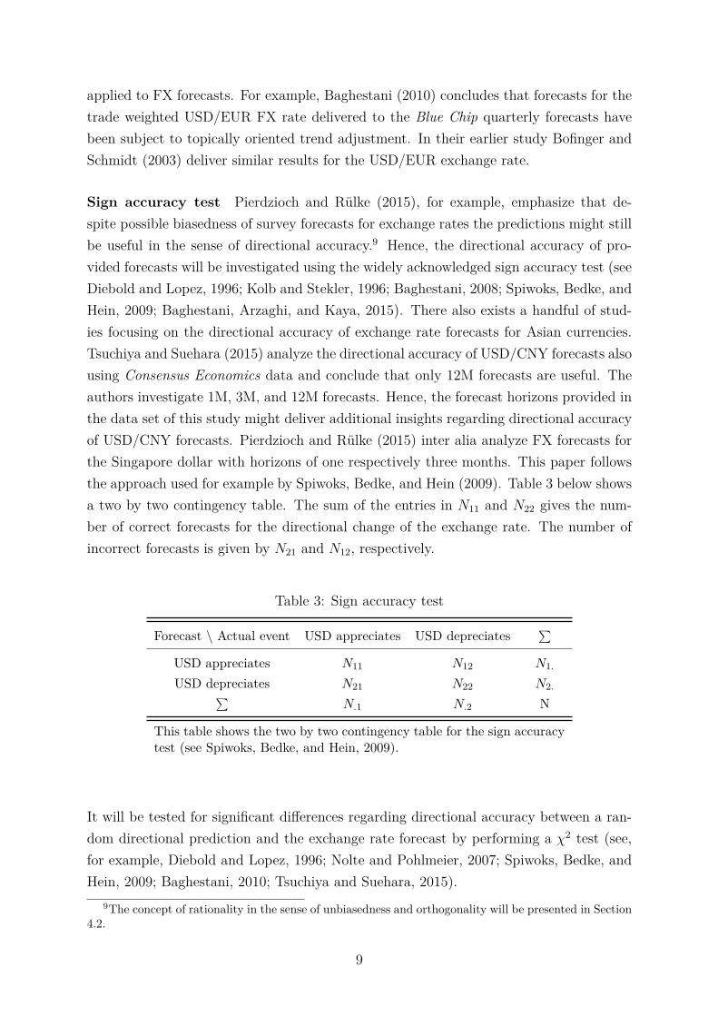
the approach used for example by Spiwoks, Bedke, and Hein (2009). Table 3 below shows

a two by two contingency table. The sum of the entries in N11 and N22 gives the num-

ber of correct forecasts for the directional change of the exchange rate. The number of

incorrect forecasts is given by N21 and N12, respectively.

Table 3: Sign accuracy test

Forecast \ Actual event USD appreciates USD depreciates∑

USD appreciates N11 N12 N1.

USD depreciates N21 N22 N2.∑

N.1 N.2 N

This table shows the two by two contingency table for the sign accuracytest (see Spiwoks, Bedke, and Hein, 2009).

It will be tested for significant differences regarding directional accuracy between a ran-

dom directional prediction and the exchange rate forecast by performing a χ2 test (see,

for example, Diebold and Lopez, 1996; Nolte and Pohlmeier, 2007; Spiwoks, Bedke, and

Hein, 2009; Baghestani, 2010; Tsuchiya and Suehara, 2015).

9The concept of rationality in the sense of unbiasedness and orthogonality will be presented in Section4.2.

9

4.2. Rationality of foreign exchange forecasts

Finally, the rationality of predictions is an important attribute in the context of

forecast evaluation. This is also true for exchange rate predictions. In the case of the

USD/JPY exchange rate, for example, Frenkel, Rülke, and Stadtmann (2009) test for

the rationality of FX survey forecasts by applying two criteria – namely, unbiasedness

and orthogonality (i.e. efficiency). These criteria are common measures in the literature

dealing with forecast evaluation (see also Ito, 1990; MacDonald and Marsh, 1996) and,

hence, will be applied in this paper as well.

Test for unbiasedness Firstly, the test for unbiasedness will be used (see, for example,

Hafer, Hein, and MacDonald, 1992, who apply the test for unbiasedness for futures market

quotes, forward rates and survey forecasts for interest rates). Audretsch and Stadtmann

(2005), Frenkel, Rülke, and Stadtmann (2009), Frenkel, Mauch, Rülke, et al. (2017), as

well as Ince and Molodtsova (2017) investigate whether survey forecasts are unbiased

predictors of future FX rates and come to different conclusions. Following, for example,

Chinn and Frankel (1994), and more recently Ince and Molodtsova (2017) a simple linear

regression model with the actual exchange rate change (st+h − st) as dependent variable

and the expected exchange rate change (st+h − st) as the independent variable will be

estimated, where st is the log of the price of one US dollar in the foreign currency and

the forecast of the exchanges at t for the horizon h is given as st+h (with the forecast

horizons h = 3, 12, or 24 months).10 The error term is given by ut+h. For the test for

unbiasedness the joint H0 : α = 0 and β = 1 has to be empirically verified respectively

discarded (see, once again, Ince and Molodtsova, 2017).11

st+h − st = α + β(st+h − st) + ut+h (3)

Test for efficiency To test for orthogonality (see, for example, Frenkel, Rülke, and

Stadtmann, 2009) the test for efficiency will be used. This test is also widely used in the

context of forecast evaluation (see inter alia Simon, 1989; Leitner and Schmidt, 2006).

Using this procedure, it is possible to verify whether the forecast errors are not related

to information available at the forecast date (see Nordhaus, 1987; Frenkel, Rülke, and

Stadtmann, 2009; Pancotto, Pericoli, and Pistagnesi, 2014; Frenkel, Mauch, Rülke, et al.,

2017). Within the empirically context of this paper this information will be represented

10Due to the non-stationarity of the USD/CNY, USD/JPY, and USD/SGD exchange rates and corre-sponding forecasts regressions in levels would lead to distorted results (see Granger and Newbold, 1974;Mitchell and Pearce, 2007). Notwithstanding, due to the stationarity of the USD/HKD FX rate and thecorresponding forecasts, to test for unbiasedness in the case of the USD/HKD forecasts, the test will beexecuted in levels.

11In addition to that null hypothesis the residuals of the linear model have to be tested for autocor-relation. The widely acknowledged Durbin Watson (DW) test is applied here (see Durbin and Watson,1950, 1951)

10

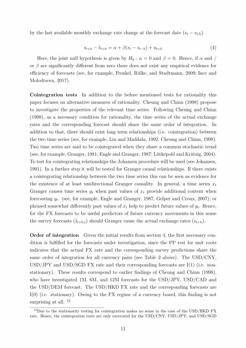
by the last available monthly exchange rate change at the forecast date (st − st-h).

st+h − st+h = α + β(st − st−h) + ut+h (4)

Here, the joint null hypothesis is given by H0 : α = 0 and β = 0. Hence, if α and /

or β are significantly different from zero there does not exist any empirical evidence for

efficiency of forecasts (see, for example, Frenkel, Rülke, and Stadtmann, 2009; Ince and

Molodtsova, 2017).

Cointegration tests In addition to the before mentioned tests for rationality this

paper focuses on alternative measures of rationality. Cheung and Chinn (1998) propose

to investigate the properties of the relevant time series. Following Cheung and Chinn

(1998), as a necessary condition for rationality, the time series of the actual exchange

rates and the corresponding forecast should share the same order of integration. In

addition to that, there should exist long term relationships (i.e. cointegration) between

the two time series (see, for example, Liu and Maddala, 1992; Cheung and Chinn, 1998).

Two time series are said to be cointegrated when they share a common stochastic trend

(see, for example, Granger, 1981; Engle and Granger, 1987; Lütkepohl and Krätzig, 2004).

To test for cointegrating relationships the Johansen procedure will be used (see Johansen,

1991). In a further step it will be tested for Granger causal relationships. If there exists

a cointegrating relationship between the two time series this can be seen as evidence for

the existence of at least unidirectional Granger causality. In general, a time series xt

Granger causes time series yt when past values of xt provide additional content when

forecasting yt. (see, for example, Engle and Granger, 1987; Gelper and Croux, 2007); or

phrased somewhat differently past values of xt help to predict future values of yt. Hence,

for the FX forecasts to be useful predictors of future currency movements in this sense

the survey forecasts (st+h,t) should Granger cause the actual exchange rates (st+h).

Order of integration Given the initial results from section 4, the first necessary con-

dition is fulfilled for the forecasts under investigation, since the PP test for unit roots

indicates that the actual FX rate and the corresponding survey predictions share the

same order of integration for all currency pairs (see Table 2 above). The USD/CNY,

USD/JPY and USD/SGD FX rate and their corresponding forecasts are I(1) (i.e. non-

stationary). These results correspond to earlier findings of Cheung and Chinn (1998),

who have investigated 1M, 6M, and 12M forecasts for the USD/JPY, USD/CAD and

the USD/DEM forecast. The USD/HKD FX rate and the corresponding forecasts are

I(0) (i.e. stationary). Owing to the FX regime of a currency board, this finding is not

surprising at all. 12

12Due to the stationarity testing for cointegration makes no sense in the case of the USD/HKD FXrate. Hence, the cointegration tests are only excecuted for the USD/CNY, USD/JPY, and USD/SGD

11

5. Empirical evidence

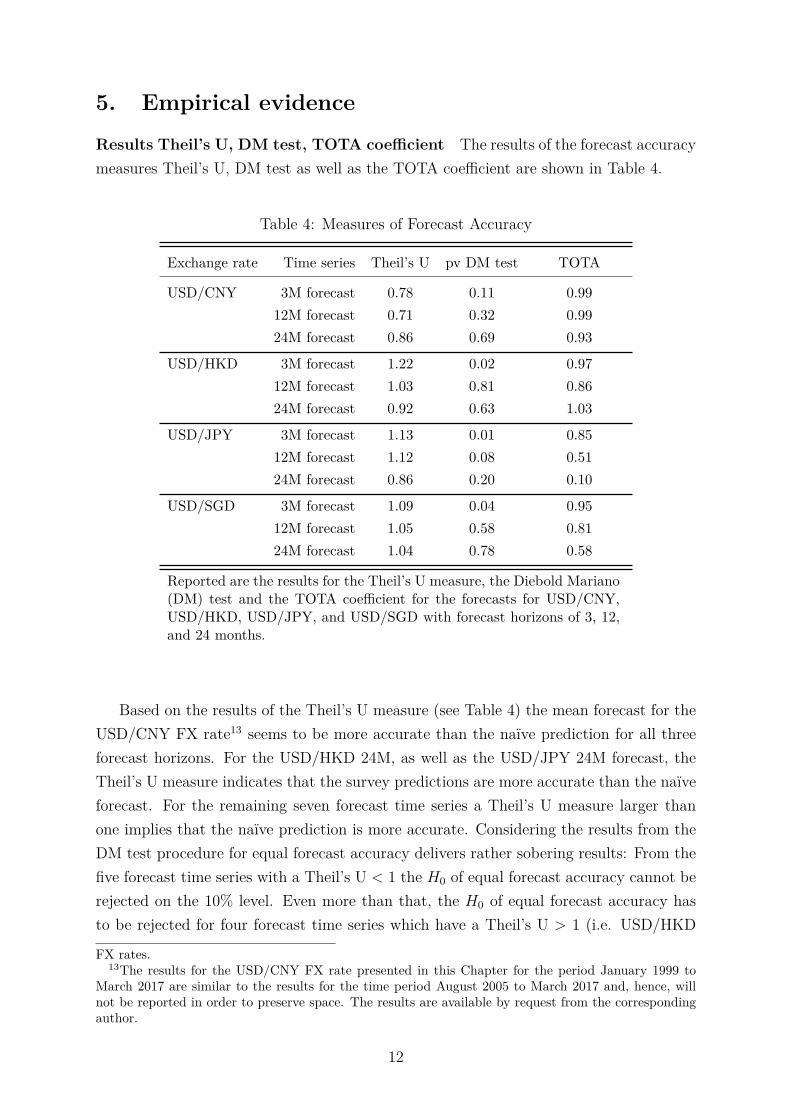
Results Theil’s U, DM test, TOTA coefficient The results of the forecast accuracy

measures Theil’s U, DM test as well as the TOTA coefficient are shown in Table 4.

Table 4: Measures of Forecast Accuracy

Exchange rate Time series Theil’s U pv DM test TOTA

USD/CNY 3M forecast 0.78 0.11 0.99

12M forecast 0.71 0.32 0.99

24M forecast 0.86 0.69 0.93

USD/HKD 3M forecast 1.22 0.02 0.97

12M forecast 1.03 0.81 0.86

24M forecast 0.92 0.63 1.03

USD/JPY 3M forecast 1.13 0.01 0.85

12M forecast 1.12 0.08 0.51

24M forecast 0.86 0.20 0.10

USD/SGD 3M forecast 1.09 0.04 0.95

12M forecast 1.05 0.58 0.81

24M forecast 1.04 0.78 0.58

Reported are the results for the Theil’s U measure, the Diebold Mariano(DM) test and the TOTA coefficient for the forecasts for USD/CNY,USD/HKD, USD/JPY, and USD/SGD with forecast horizons of 3, 12,and 24 months.

Based on the results of the Theil’s U measure (see Table 4) the mean forecast for the

USD/CNY FX rate13 seems to be more accurate than the naïve prediction for all three

forecast horizons. For the USD/HKD 24M, as well as the USD/JPY 24M forecast, the

Theil’s U measure indicates that the survey predictions are more accurate than the naïve

forecast. For the remaining seven forecast time series a Theil’s U measure larger than

one implies that the naïve prediction is more accurate. Considering the results from the

DM test procedure for equal forecast accuracy delivers rather sobering results: From the

five forecast time series with a Theil’s U < 1 the H0 of equal forecast accuracy cannot be

rejected on the 10% level. Even more than that, the H0 of equal forecast accuracy has

to be rejected for four forecast time series which have a Theil’s U > 1 (i.e. USD/HKD

FX rates.13The results for the USD/CNY FX rate presented in this Chapter for the period January 1999 to

March 2017 are similar to the results for the time period August 2005 to March 2017 and, hence, willnot be reported in order to preserve space. The results are available by request from the correspondingauthor.

12

3M, USD/JPY 3M, USD/JPY 12M and USD/SGD 3M). Hence, especially in the case

of shorter forecast horizons, the naïve predictions seems to be the superior forecast.

Interestingly, the superiority of the naïve predicition seems to be regime independent.

As regards topically oriented trend adjustments, the only TOTA coefficient > 1 belongs

to the USD/HKD 24M forecast. Especially in the case of the USD/JPY forecasts, the

topically oriented forecasting behavior becomes obvious (i.e. TOTA = 0.10).

Results sign accuracy test The results of the sign accuracy test are presented in

Table 5 below. On the 5%-level the USD/CNY as well as the USD/HKD forecasts are

significantly better than a random forecast for all three forecast horizons. Hence, the

results contradict the earlier findings of Tsuchiya and Suehara (2015). For the USD/JPY

and USD/SGD predictions the results are more heterogeneous. For the 3M forecast for

the USD/JPY as well as the USD/SGD no statistically significant difference from the

random prediction regarding the sign accuracy has been found. The USD/JPY 12M

forecast is worse than a random prediction for the direction of change, whereas the 12M

forecast for USD/SGD outperforms the random prediction. The 24M forecasts both for

the USD/JPY and for USD/SGD are better than a random prediction. As regards the

regime dependent quality of FX forecasts it is noteworthy that the USD/CNY exchange

rate as well as the USD/HKD exchange rate forecasts are consistently more sign accurate

than the random prediction.

13

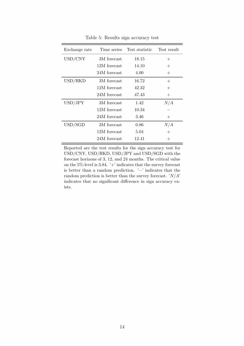
Table 5: Results sign accuracy test

Exchange rate Time series Test statistic Test result

USD/CNY 3M forecast 18.15 +

12M forecast 14.10 +

24M forecast 4.00 +

USD/HKD 3M forecast 16.72 +

12M forecast 42.32 +

24M forecast 47.43 +

USD/JPY 3M forecast 1.42 N/A

12M forecast 10.34 −

24M forecast 3.46 +

USD/SGD 3M forecast 0.86 N/A

12M forecast 5.04 +

24M forecast 12.41 +

Reported are the test results for the sign accuracy test forUSD/CNY, USD/HKD, USD/JPY and USD/SGD with theforecast horizons of 3, 12, and 24 months. The critical valueon the 5%-level is 3.84. ’+’ indicates that the survey forecastis better than a random prediction. ’−’ indicates that therandom prediction is better than the survey forecast. ’N/A’indicates that no significant difference in sign accuracy ex-ists.

14

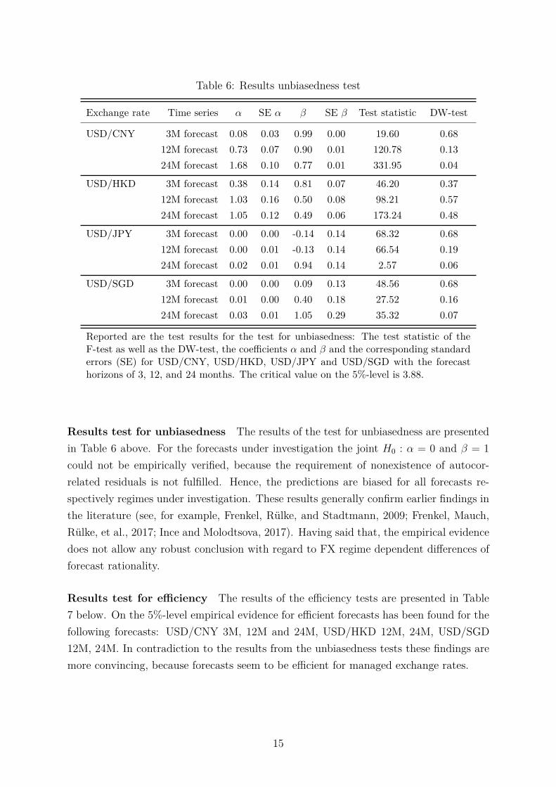
Table 6: Results unbiasedness test

Exchange rate Time series α SE α β SE β Test statistic DW-test

USD/CNY 3M forecast 0.08 0.03 0.99 0.00 19.60 0.68

12M forecast 0.73 0.07 0.90 0.01 120.78 0.13

24M forecast 1.68 0.10 0.77 0.01 331.95 0.04

USD/HKD 3M forecast 0.38 0.14 0.81 0.07 46.20 0.37

12M forecast 1.03 0.16 0.50 0.08 98.21 0.57

24M forecast 1.05 0.12 0.49 0.06 173.24 0.48

USD/JPY 3M forecast 0.00 0.00 -0.14 0.14 68.32 0.68

12M forecast 0.00 0.01 -0.13 0.14 66.54 0.19

24M forecast 0.02 0.01 0.94 0.14 2.57 0.06

USD/SGD 3M forecast 0.00 0.00 0.09 0.13 48.56 0.68

12M forecast 0.01 0.00 0.40 0.18 27.52 0.16

24M forecast 0.03 0.01 1.05 0.29 35.32 0.07

Reported are the test results for the test for unbiasedness: The test statistic of theF-test as well as the DW-test, the coefficients α and β and the corresponding standarderrors (SE) for USD/CNY, USD/HKD, USD/JPY and USD/SGD with the forecasthorizons of 3, 12, and 24 months. The critical value on the 5%-level is 3.88.

Results test for unbiasedness The results of the test for unbiasedness are presented

in Table 6 above. For the forecasts under investigation the joint H0 : α = 0 and β = 1

could not be empirically verified, because the requirement of nonexistence of autocor-

related residuals is not fulfilled. Hence, the predictions are biased for all forecasts re-

spectively regimes under investigation. These results generally confirm earlier findings in

the literature (see, for example, Frenkel, Rülke, and Stadtmann, 2009; Frenkel, Mauch,

Rülke, et al., 2017; Ince and Molodtsova, 2017). Having said that, the empirical evidence

does not allow any robust conclusion with regard to FX regime dependent differences of

forecast rationality.

Results test for efficiency The results of the efficiency tests are presented in Table

7 below. On the 5%-level empirical evidence for efficient forecasts has been found for the

following forecasts: USD/CNY 3M, 12M and 24M, USD/HKD 12M, 24M, USD/SGD

12M, 24M. In contradiction to the results from the unbiasedness tests these findings are

more convincing, because forecasts seem to be efficient for managed exchange rates.

15

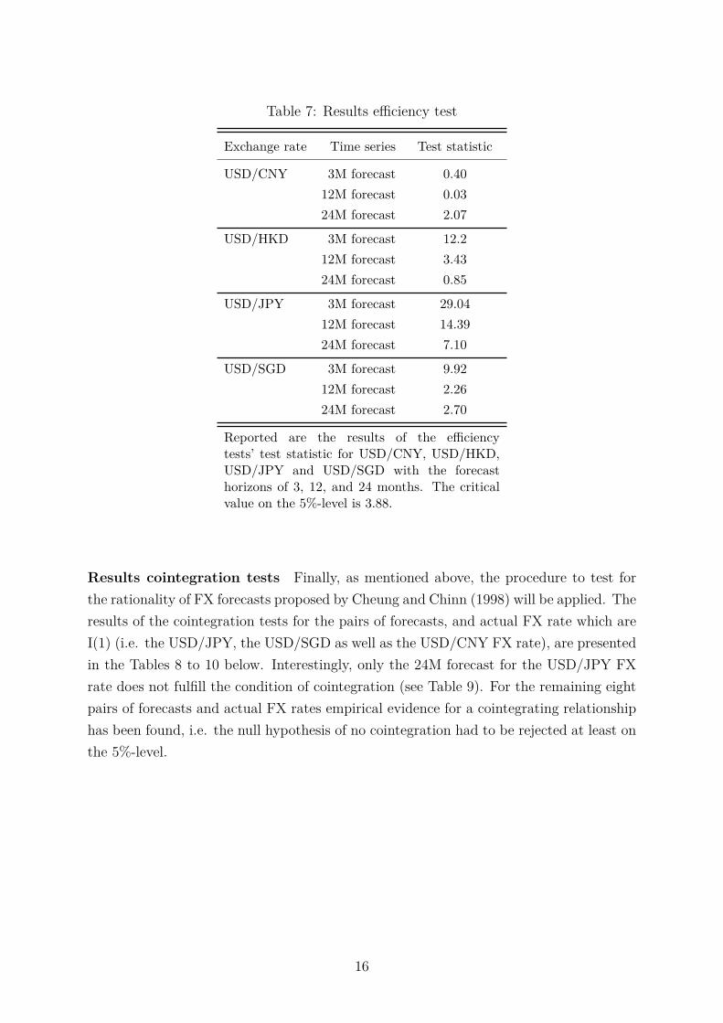
Table 7: Results efficiency test

Exchange rate Time series Test statistic

USD/CNY 3M forecast 0.40

12M forecast 0.03

24M forecast 2.07

USD/HKD 3M forecast 12.2

12M forecast 3.43

24M forecast 0.85

USD/JPY 3M forecast 29.04

12M forecast 14.39

24M forecast 7.10

USD/SGD 3M forecast 9.92

12M forecast 2.26

24M forecast 2.70

Reported are the results of the efficiencytests’ test statistic for USD/CNY, USD/HKD,USD/JPY and USD/SGD with the forecasthorizons of 3, 12, and 24 months. The criticalvalue on the 5%-level is 3.88.

Results cointegration tests Finally, as mentioned above, the procedure to test for

the rationality of FX forecasts proposed by Cheung and Chinn (1998) will be applied. The

results of the cointegration tests for the pairs of forecasts, and actual FX rate which are

I(1) (i.e. the USD/JPY, the USD/SGD as well as the USD/CNY FX rate), are presented

in the Tables 8 to 10 below. Interestingly, only the 24M forecast for the USD/JPY FX

rate does not fulfill the condition of cointegration (see Table 9). For the remaining eight

pairs of forecasts and actual FX rates empirical evidence for a cointegrating relationship

has been found, i.e. the null hypothesis of no cointegration had to be rejected at least on

the 5%-level.

16

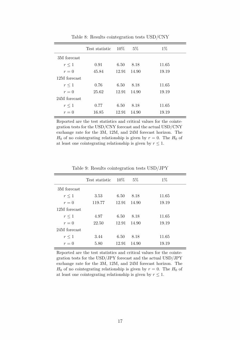
Table 8: Results cointegration tests USD/CNY

Test statistic 10% 5% 1%

3M forecast

r ≤ 1 0.91 6.50 8.18 11.65

r = 0 45.84 12.91 14.90 19.19

12M forecast

r ≤ 1 0.76 6.50 8.18 11.65

r = 0 25.62 12.91 14.90 19.19

24M forecast

r ≤ 1 0.77 6.50 8.18 11.65

r = 0 16.85 12.91 14.90 19.19

Reported are the test statistics and critical values for the cointe-gration tests for the USD/CNY forecast and the actual USD/CNYexchange rate for the 3M, 12M, and 24M forecast horizon. TheH0 of no cointegrating relationship is given by r = 0. The H0 ofat least one cointegrating relationship is given by r ≤ 1.

Table 9: Results cointegration tests USD/JPY

Test statistic 10% 5% 1%

3M forecast

r ≤ 1 3.53 6.50 8.18 11.65

r = 0 119.77 12.91 14.90 19.19

12M forecast

r ≤ 1 4.97 6.50 8.18 11.65

r = 0 22.50 12.91 14.90 19.19

24M forecast

r ≤ 1 3.44 6.50 8.18 11.65

r = 0 5.80 12.91 14.90 19.19

Reported are the test statistics and critical values for the cointe-gration tests for the USD/JPY forecast and the actual USD/JPYexchange rate for the 3M, 12M, and 24M forecast horizon. TheH0 of no cointegrating relationship is given by r = 0. The H0 ofat least one cointegrating relationship is given by r ≤ 1.

17

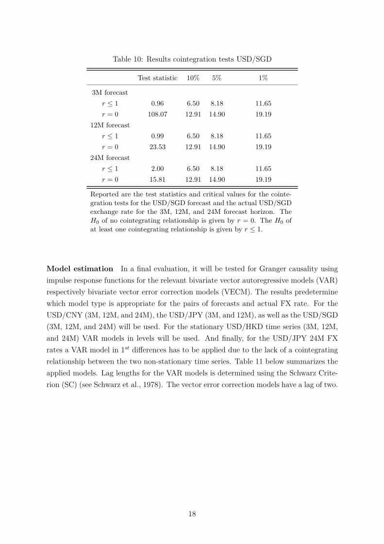
Table 10: Results cointegration tests USD/SGD

Test statistic 10% 5% 1%

3M forecast

r ≤ 1 0.96 6.50 8.18 11.65

r = 0 108.07 12.91 14.90 19.19

12M forecast

r ≤ 1 0.99 6.50 8.18 11.65

r = 0 23.53 12.91 14.90 19.19

24M forecast

r ≤ 1 2.00 6.50 8.18 11.65

r = 0 15.81 12.91 14.90 19.19

Reported are the test statistics and critical values for the cointe-gration tests for the USD/SGD forecast and the actual USD/SGDexchange rate for the 3M, 12M, and 24M forecast horizon. TheH0 of no cointegrating relationship is given by r = 0. The H0 ofat least one cointegrating relationship is given by r ≤ 1.

Model estimation In a final evaluation, it will be tested for Granger causality using

impulse response functions for the relevant bivariate vector autoregressive models (VAR)

respectively bivariate vector error correction models (VECM). The results predetermine

which model type is appropriate for the pairs of forecasts and actual FX rate. For the

USD/CNY (3M, 12M, and 24M), the USD/JPY (3M, and 12M), as well as the USD/SGD

(3M, 12M, and 24M) will be used. For the stationary USD/HKD time series (3M, 12M,

and 24M) VAR models in levels will be used. And finally, for the USD/JPY 24M FX

rates a VAR model in 1st differences has to be applied due to the lack of a cointegrating

relationship between the two non-stationary time series. Table 11 below summarizes the

applied models. Lag lengths for the VAR models is determined using the Schwarz Crite-

rion (SC) (see Schwarz et al., 1978). The vector error correction models have a lag of two.

18

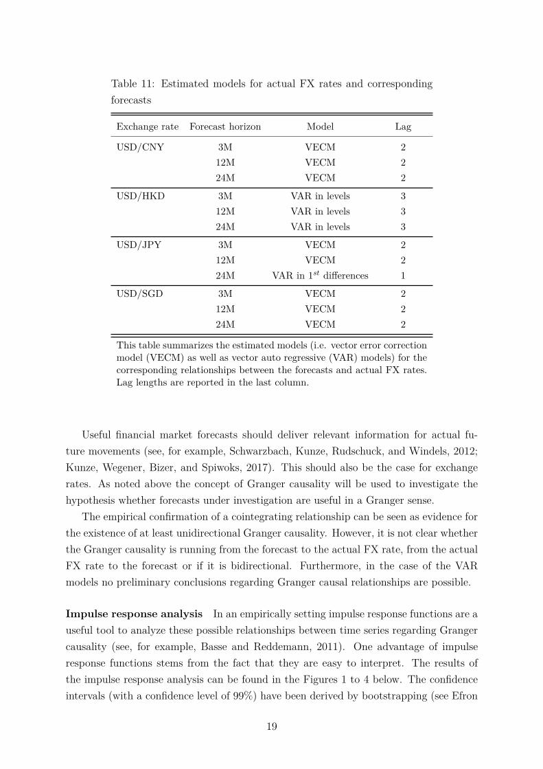
Table 11: Estimated models for actual FX rates and corresponding

forecasts

Exchange rate Forecast horizon Model Lag

USD/CNY 3M VECM 2

12M VECM 2

24M VECM 2

USD/HKD 3M VAR in levels 3

12M VAR in levels 3

24M VAR in levels 3

USD/JPY 3M VECM 2

12M VECM 2

24M VAR in 1st differences 1

USD/SGD 3M VECM 2

12M VECM 2

24M VECM 2

This table summarizes the estimated models (i.e. vector error correctionmodel (VECM) as well as vector auto regressive (VAR) models) for thecorresponding relationships between the forecasts and actual FX rates.Lag lengths are reported in the last column.

Useful financial market forecasts should deliver relevant information for actual fu-

ture movements (see, for example, Schwarzbach, Kunze, Rudschuck, and Windels, 2012;

Kunze, Wegener, Bizer, and Spiwoks, 2017). This should also be the case for exchange

rates. As noted above the concept of Granger causality will be used to investigate the

hypothesis whether forecasts under investigation are useful in a Granger sense.

The empirical confirmation of a cointegrating relationship can be seen as evidence for

the existence of at least unidirectional Granger causality. However, it is not clear whether

the Granger causality is running from the forecast to the actual FX rate, from the actual

FX rate to the forecast or if it is bidirectional. Furthermore, in the case of the VAR

models no preliminary conclusions regarding Granger causal relationships are possible.

Impulse response analysis In an empirically setting impulse response functions are a

useful tool to analyze these possible relationships between time series regarding Granger

causality (see, for example, Basse and Reddemann, 2011). One advantage of impulse

response functions stems from the fact that they are easy to interpret. The results of

the impulse response analysis can be found in the Figures 1 to 4 below. The confidence

intervals (with a confidence level of 99%) have been derived by bootstrapping (see Efron

19

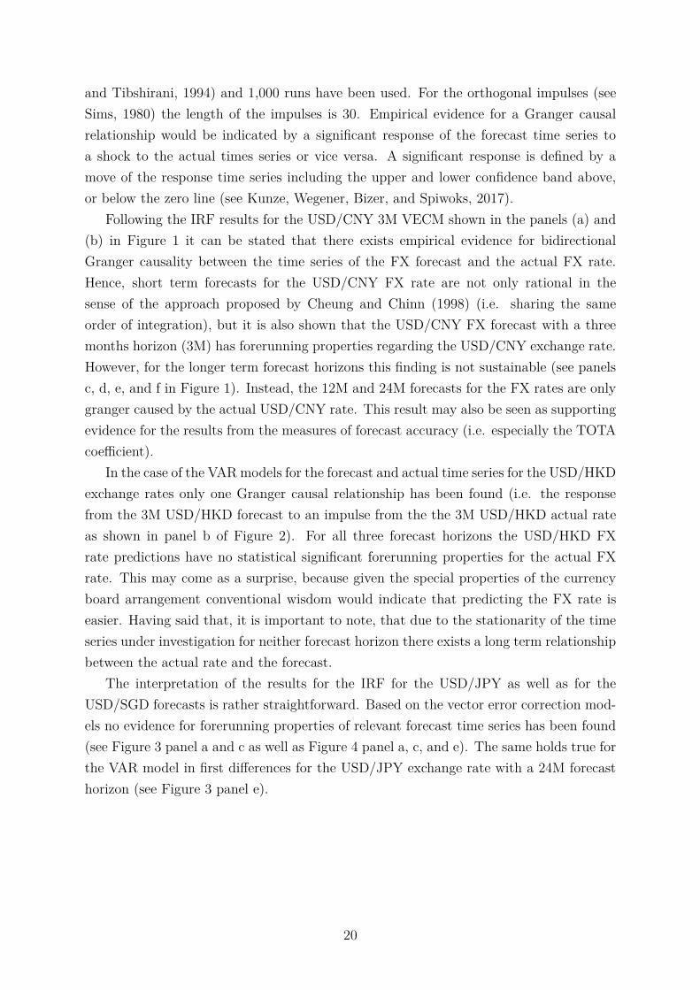
and Tibshirani, 1994) and 1,000 runs have been used. For the orthogonal impulses (see

Sims, 1980) the length of the impulses is 30. Empirical evidence for a Granger causal

relationship would be indicated by a significant response of the forecast time series to

a shock to the actual times series or vice versa. A significant response is defined by a

move of the response time series including the upper and lower confidence band above,

or below the zero line (see Kunze, Wegener, Bizer, and Spiwoks, 2017).

Following the IRF results for the USD/CNY 3M VECM shown in the panels (a) and

(b) in Figure 1 it can be stated that there exists empirical evidence for bidirectional

Granger causality between the time series of the FX forecast and the actual FX rate.

Hence, short term forecasts for the USD/CNY FX rate are not only rational in the

sense of the approach proposed by Cheung and Chinn (1998) (i.e. sharing the same

order of integration), but it is also shown that the USD/CNY FX forecast with a three

months horizon (3M) has forerunning properties regarding the USD/CNY exchange rate.

However, for the longer term forecast horizons this finding is not sustainable (see panels

c, d, e, and f in Figure 1). Instead, the 12M and 24M forecasts for the FX rates are only

granger caused by the actual USD/CNY rate. This result may also be seen as supporting

evidence for the results from the measures of forecast accuracy (i.e. especially the TOTA

coefficient).

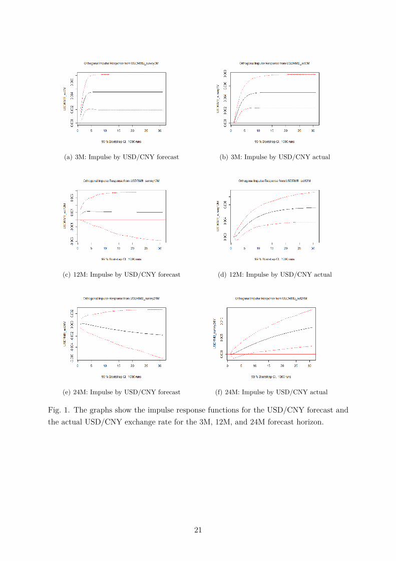
In the case of the VAR models for the forecast and actual time series for the USD/HKD

exchange rates only one Granger causal relationship has been found (i.e. the response

from the 3M USD/HKD forecast to an impulse from the the 3M USD/HKD actual rate

as shown in panel b of Figure 2). For all three forecast horizons the USD/HKD FX

rate predictions have no statistical significant forerunning properties for the actual FX

rate. This may come as a surprise, because given the special properties of the currency

board arrangement conventional wisdom would indicate that predicting the FX rate is

easier. Having said that, it is important to note, that due to the stationarity of the time

series under investigation for neither forecast horizon there exists a long term relationship

between the actual rate and the forecast.

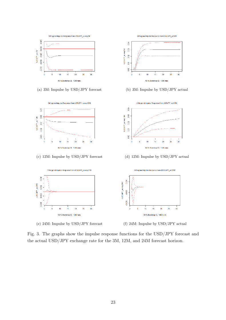
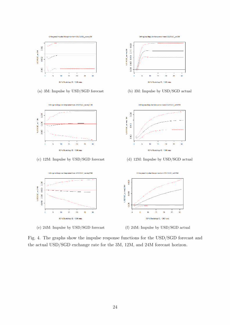
The interpretation of the results for the IRF for the USD/JPY as well as for the

USD/SGD forecasts is rather straightforward. Based on the vector error correction mod-

els no evidence for forerunning properties of relevant forecast time series has been found

(see Figure 3 panel a and c as well as Figure 4 panel a, c, and e). The same holds true for

the VAR model in first differences for the USD/JPY exchange rate with a 24M forecast

horizon (see Figure 3 panel e).

20

(a) 3M: Impulse by USD/CNY forecast (b) 3M: Impulse by USD/CNY actual

(c) 12M: Impulse by USD/CNY forecast (d) 12M: Impulse by USD/CNY actual

(e) 24M: Impulse by USD/CNY forecast (f) 24M: Impulse by USD/CNY actual

Fig. 1. The graphs show the impulse response functions for the USD/CNY forecast and

the actual USD/CNY exchange rate for the 3M, 12M, and 24M forecast horizon.

21

(a) 3M: Impulse by USD/HKD forecast (b) 3M: Impulse by USD/HKD actual

(c) 12M: Impulse by USD/HKD forecast (d) 12M: Impulse by USD/HKD actual

(e) 24M: Impulse by USD/HKD forecast (f) 24M: Impulse by USD/HKD actual

Fig. 2. The graphs show the impulse response functions for the USD/HKD forecast and

the actual USD/HKD exchange rate for the 3M, 12M, and 24M forecast horizon.

22

(a) 3M: Impulse by USD/JPY forecast (b) 3M: Impulse by USD/JPY actual

(c) 12M: Impulse by USD/JPY forecast (d) 12M: Impulse by USD/JPY actual

(e) 24M: Impulse by USD/JPY forecast (f) 24M: Impulse by USD/JPY actual

Fig. 3. The graphs show the impulse response functions for the USD/JPY forecast and

the actual USD/JPY exchange rate for the 3M, 12M, and 24M forecast horizon.

23

(a) 3M: Impulse by USD/SGD forecast (b) 3M: Impulse by USD/SGD actual

(c) 12M: Impulse by USD/SGD forecast (d) 12M: Impulse by USD/SGD actual

(e) 24M: Impulse by USD/SGD forecast (f) 24M: Impulse by USD/SGD actual

Fig. 4. The graphs show the impulse response functions for the USD/SGD forecast and

the actual USD/SGD exchange rate for the 3M, 12M, and 24M forecast horizon.

24

6. Conclusions

In this paper monthly survey based exchange rate forecasts for the exchange rates

of the Chinese yuan, the Hong Kong dollar, the Japanese yen as well as the Singapore

dollar vis-à-vis the US dollar have been investigated regarding accuracy and rationality.

Thereby, some interesting and relevant general results are worth mentioning. Rather

strong empirical evidence for topically orientated (TOTA) forecasting behavior for all

four exchange rates has been found. Furthermore, especially for shorter forecast horizons

(i.e. 3M) the naïve no change prediction seems to outperform the survey forecasts with

the three months forecasts for the USD/CNY exchange rate being the only exception.

As regards sign accuracy for the forecasts for the USD/CNY and USD/HKD, empirical

evidence supports the conclusion that the survey forecasts are more precise than a random

prediction for all three forecast horizons under investigation. These results have been

supported by the test for efficiency. Having said that, empirical evidence shows that all

forecasts are irrational in the sense of the test for unbiasedness, due to the existence of

autocorrelated residuals.

Applying an alternative framework to test for rationality proposed by Cheung and

Chinn (1998), it has been shown that, for all four currency regimes the forecasts and

actual exchange rates share the same order of integration. Furthermore, for the foreign

exchange regimes with I(1) time series (i.e. USD/CNY, USD/JPY, and USD/SGD) em-

pirical evidence supports the hypothesis of the existence of cointegrating relationships

and, hence, a long term relation has been statistically validated. The only exception has

been the USD/JPY forecast with a forecast horizon of 24 months. However, impulse

response analysis for all currency regimes under investigation indicated that only the

three months forecast for the managed USD/CNY exchange rate has forerunning prop-

erties. More generally, forerunning properties of the remaining survey forecasts under

investigation are rather limited.

Furthermore, as regards regime dependent differences with respect to accuracy and

rationality it has not been shown that exchange rates for fixed or closely managed ex-

change rates are in general easier to forecast. Despite the fact that no definite conclusion

regarding FX regime dependent forecast accuracy respectively rationality of the survey

predictions is suitable, the presented empirical evidence indicates that the forecasts for

the managed Chinese exchange rate systems are closest to be being rational and fore-

running, especially for the three months forecast horizons. Furthermore, also taking into

account the results for the forecast evaluation of the USD/HKD exchange rate it can be

stated that forecast accuracy – especially when it comes to sign accuracy – seems to be

higher for stronger controlled exchange rate regimes. These findings are relevant both for

the recipients of foreign exchange forecasts (e.g. corporate managers or politicians) and

for the monetary respectively FX policy makers themselves.

25

After all, these findings may not be extraordinary surprising, as in managed foreign

exchange regimes monetary policy authorities have to follow a self or government obliged

framework. However, it has to be taken into account, that strongly regulated FX markets

may be much more exposed to event risks and tail events, respectively, like for example

currency crisis and, most importantly in the context of the results of this study, shifts in

the FX regimes (see, for example, Husain, Mody, and Rogoff, 2005; Fiess and Shankar,

2009; Abildgren, 2014). Having said that, further research is necessary and should, par-

ticularly, focus on the predictability of regime shifts in managed exchange rate systems

and currency boards, the credibility of fixed exchange rate regimes as well as the influence

thereof on forecast accuracy and rationality, respectively.

26

References

Abildgren, K., 2014. Tail events in the FX markets since 1740. The Journal of Risk

Finance 15, 294–311.

Aggarwal, R., 2013. Corporate management of foreign currency risk: Conceptual frame-

work, policies, and strategies. International Finance: A Survey p. 447.

Aggarwal, R., Chen, X., Yur-Austin, J., 2011. Currency risk exposure of Chinese corpo-

rations. Research in International Business and Finance 25, 266–276.

Ahmed, S., Liu, X., Valente, G., 2016. Can currency-based risk factors help forecast

exchange rates? International Journal of Forecasting 32, 75–97.

Andres, P., Spiwoks, M., 1999. Forecast quality matrix: A methodological survey of

judging forecast quality of capital market forecasts. Journal of Economics and Statistics

(Jahrbuecher fuer Nationaloekonomie und Statistik) 219, 513–542.

Audretsch, D. B., Stadtmann, G., 2005. Biases in FX-forecasts: Evidence from panel

data. Global Finance Journal 16, 99–111.

Avraham, D., Ungar, M., Zilberfarb, B.-Z., 1987. Are foreign exchange forecasts rational?:

An empirical note. Economics Letters 24, 291–293.

Bacchetta, P., Mertens, E., Van Wincoop, E., 2009. Predictability in financial markets:

What do survey expectations tell us? Journal of International Money and Finance 28,

406–426.

Baghestani, H., 2008. Federal Reserve versus private information: Who is the best un-

employment rate predictor? Journal of Policy Modeling 30, 101–110.

Baghestani, H., 2010. Evaluating Blue Chip forecasts of the trade-weighted dollar ex-

change rate. Applied Financial Economics 20, 1879–1889.

Baghestani, H., Arzaghi, M., Kaya, I., 2015. On the accuracy of Blue Chip forecasts of

interest rates and country risk premiums. Applied Economics 47, 113–122.

Basse, T., Reddemann, S., 2011. Inflation and the dividend policy of US firms. Managerial

Finance 37, 34–46.

Beckmann, J., Czudaj, R., 2017a. Exchange rate expectations since the financial crisis:

Performance evaluation and the role of monetary policy and safe haven. Journal of

International Money and Finance 74, 283–300.

Beckmann, J., Czudaj, R., 2017b. The impact of uncertainty on professional exchange

rate forecasts. Journal of International Money and Finance 73, 296–316.

27

Beine, M., Bénassy-Quéré, A., MacDonald, R., 2007. The impact of central bank interven-

tion on exchange-rate forecast heterogeneity. Journal of the Japanese and International

Economies 21, 38–63.

Bofinger, P., Schmidt, R., 2003. On the reliability of professional exchange rate forecasts.

Financial Markets and Portfolio Management 17, 437–449.

Bordo, M. D., Choudhri, E. U., Fazio, G., MacDonald, R., 2017. The real exchange rate in

the long run: Balassa-Samuelson effects reconsidered. Journal of International Money

and Finance 75, 69–92.

Byrne, J. P., Korobilis, D., Ribeiro, P. J., 2016. Exchange rate predictability in a changing

world. Journal of International Money and Finance 62, 1–24.

Calvo, G. A., Reinhart, C. M., 2002. Fear of floating. The Quarterly Journal of Economics

117, 379–408.

Cheung, Y.-W., Chinn, M. D., 1998. Integration, cointegration and the forecast consis-

tency of structural exchange rate models. Journal of International Money and Finance

17, 813–830.

Cheung, Y.-W., Chinn, M. D., Fujii, E., 2007. The overvaluation of renminbi undervalu-

ation. Journal of International Money and Finance 26, 762–785.

Cheung, Y.-W., Hui, C.-H., Tsang, A., 2016. The Renminbi central parity: An empirical

investigation. CESifo Working Paper No. 5963 .

Cheung, Y.-W., Hui, C.-H., Tsang, A., 2017. The RMB central parity formation mech-

anism after august 2015: A statistical analysis. HKIMR Working Paper No. 06/2017

.

Chinn, M., Frankel, J., 1994. Patterns in exchange rate forecasts for twenty-five curren-

cies. Journal of Money, Credit and Banking 26, 759–770.

Chit, M. M., Rizov, M., Willenbockel, D., 2010. Exchange rate volatility and exports:

New empirical evidence from the emerging East Asian economies. The World Economy

33, 239–263.

Chow, H.-K., 2007. Singapore’s exchange rate policy: Some implementation issues. The

Singapore Economic Review 52, 445–458.

Chow, H. K., Lim, G., McNelis, P. D., 2014. Monetary regime choice in Singapore: Would

a Taylor rule outperform exchange-rate management? Journal of Asian Economics 30,

63–81.

28

Cook, D., Yetman, J., 2014. Currency boards when interest rates are zero. Pacific Eco-

nomic Review 19, 135–151.

De Grauwe, P., Markiewicz, A., 2013. Learning to forecast the exchange rate: Two

competing approaches. Journal of International Money and Finance 32, 42–76.

Devereux, M. B., 2003. A tale of two currencies: The Asian crisis and the exchange rate

regimes of Hong Kong and Singapore. Review of International Economics 11, 38–54.

Dick, C. D., MacDonald, R., Menkhoff, L., 2015. Exchange rate forecasts and expected

fundamentals. Journal of International Money and Finance 53, 235–256.

Diebold, F. X., Lopez, J. A., 1996. 8 forecast evaluation and combination. Handbook of

statistics 14, 241–268.

Diebold, F. X., Mariano, R. S., 1995. Comparing predictive accuracy. Journal of Business

& Economic Statistics 13, 253–263.

Dominguez, K. M., 1986. Are foreign exchange forecasts rational?: New evidence from

survey data. Economics Letters 21, 277–281.

Dreger, C., Stadtmann, G., 2008. What drives heterogeneity in foreign exchange rate ex-

pectations: Insights from a new survey. International Journal of Finance & Economics

13, 360–367.

Duffy, G., Giddy, I., 1975. The random behavior of flexible exchange rates. Journal of

International Business Studies 6, 1–32.

Dunis, C. L., Shannon, G., 2005. Emerging markets of south-east and central Asia: Do

they still offer a diversification benefit? Journal of Asset Management 6, 168–190.

Durbin, J., Watson, G., 1950. Testing for serial correlation in least squares regression-i.

Biometrika 37, 409–428.

Durbin, J., Watson, G. S., 1951. Testing for serial correlation in least squares regression.

II. Biometrika 38, 159–177.

Efron, B., Tibshirani, R. J., 1994. An introduction to the bootstrap. CRC press.

Engle, R. F., Granger, C. W., 1987. Co-integration and error correction: representation,

estimation, and testing. Econometrica: journal of the Econometric Society pp. 251–276.

Fiess, N., Shankar, R., 2009. Determinants of exchange rate regime switching. Journal of

International Money and Finance 28, 68–98.

29

Frankel, J. A., Rose, A. K., 1994. A survey of empirical research on nominal exchange

rates. Tech. rep., National Bureau of Economic Research.

Fratzscher, M., 2009. What explains global exchange rate movements during the financial

crisis? Journal of International Money and Finance 28, 1390–1407.

Frenkel, J. A., Mussa, M. L., 1980. The efficiency of foreign exchange markets and mea-

sures of turbulence. The American Economic Review 70, 374–381.

Frenkel, M., Mauch, M., Rülke, J.-C., et al., 2017. Forecaster rationality and expectation

formation in foreign exchange markets: Do emerging markets differ from industrialized

economies? Tech. rep., WHU-Otto Beisheim School of Management, Economics Group.

Frenkel, M., Rülke, J.-C., Stadtmann, G., 2009. Two currencies, one model? Evidence

from the Wall Street Journal forecast poll. Journal of International Financial Markets,

Institutions and Money 19, 588–596.

Gelper, S., Croux, C., 2007. Multivariate out-of-sample tests for Granger causality. Com-

putational statistics & data analysis 51, 3319–3329.

Granger, C. W., 1981. Some properties of time series data and their use in econometric

model specification. Journal of econometrics 16, 121–130.

Granger, C. W., Newbold, P., 1974. Spurious regressions in econometrics. Journal of

econometrics 2, 111–120.

Hafer, R. W., Hein, S. E., MacDonald, S. S., 1992. Market and survey forecasts of the

three-month treasury-bill rate. Journal of Business pp. 123–138.

Hamada, K., Hayashi, F., 1985. Monetary policy in postwar Japan. Monetary Policy in

Our Times pp. 83–121.

Hayakawa, K., Kimura, F., 2009. The effect of exchange rate volatility on international

trade in East Asia. Journal of the Japanese and International Economies 23, 395–406.

Heiden, S., Klein, C., Zwergel, B., 2013. Beyond fundamentals: Investor sentiment and

exchange rate forecasting. European Financial Management 19, 558–578.

Hernandez, L., Montiel, P. J., 2003. Post-crisis exchange rate policy in five Asian coun-

tries: Filling in the “hollow middle”? Journal of the Japanese and International

Economies 17, 336–369.

Herwartz, H., Schlüter, S., 2017. On the predictive information of futures’ prices: A

wavelet-based assessment. Journal of Forecasting 36, 345–356.

30

Ho, C., 2002. A survey of the institutional and operational aspects of modern-day currency

boards. BIS Working Paper 110.

Husain, A. M., Mody, A., Rogoff, K. S., 2005. Exchange rate regime durability and

performance in developing versus advanced economies. Journal of monetary economics

52, 35–64.

Hutchison, M., Walsh, C. E., 1992. Empirical evidence on the insulation properties of

fixed and flexible exchange rates: The Japanese experience. Journal of International

Economics 32, 241–263.

Hyndman, R. J., Koehler, A. B., 2006. Another look at measures of forecast accuracy.

International journal of forecasting 22, 679–688.

Ince, O., Molodtsova, T., 2017. Rationality and forecasting accuracy of exchange rate

expectations: Evidence from survey-based forecasts. Journal of International Financial

Markets, Institutions and Money 47, 131–151.

Ito, T., 1990. Foreign exchange rate expectations: Micro survey data. The American

Economic Review pp. 434–449.

Johansen, S., 1991. Estimation and hypothesis testing of cointegration vectors in Gaussian

vector autoregressive models. Econometrica: Journal of the Econometric Society pp.

1551–1580.

Jongen, R., Verschoor, W. F., Wolff, C. C., Zwinkels, R. C., 2012. Explaining dispersion in

foreign exchange expectations: A heterogeneous agent approach. Journal of Economic

Dynamics and Control 36, 719–735.

Kan, Y. Y., 2017. Why RMB should be more flexible. Journal of Financial Economic

Policy 9, 156–173.

Kilian, L., Taylor, M. P., 2003. Why is it so difficult to beat the random walk forecast of

exchange rates? Journal of International Economics 60, 85–107.

Klein, M. W., Shambaugh, J. C., 2008. The dynamics of exchange rate regimes: Fixes,

floats, and flips. Journal of International Economics 75, 70–92.

Kohlscheen, E., 2014. The impact of monetary policy on the exchange rate: A high

frequency exchange rate puzzle in emerging economies. Journal of International Money

and Finance 44, 69–96.

Kokenyne, A., Veyrune, R., Habermeier, M. K. F., Anderson, H., 2009. Revised system

for the classification of exchange rate arrangements. No. 9-211, International Monetary

Fund.

31

Kolb, R., Stekler, H. O., 1996. How well do analysts forecast interest rates? Journal of

Forecasting 15, 385–394.

Kunze, F., Wegener, C., Bizer, K., Spiwoks, M., 2017. Forecasting European interest

rates in times of financial crisis – What insights do we get from international survey

forecasts? Journal of International Financial Markets, Institutions and Money 48,

192–205.

Leitch, G., Tanner, J. E., 1991. Economic forecast evaluation: Profits versus the conven-

tional error measures. The American Economic Review pp. 580–590.

Leitner, J., Schmidt, R., 2006. A systematic comparison of professional exchange rate

forecasts with the judgemental forecasts of novices. Central European Journal of Op-

erations Research 14, 87–102.

Liu, P. C., Maddala, G. S., 1992. Rationality of survey data and tests for market efficiency

in the foreign exchange markets. Journal of International Money and Finance 11, 366–

381.

Lütkepohl, H., Krätzig, M., 2004. Applied time series econometrics. Cambridge university

press.

MacDonald, R., Marsh, I. W., 1996. Currency forecasters are heterogeneous: Confirma-

tion and consequences. Journal of International Money and Finance 15, 665–685.

MacDonald, R., Nagayasu, J., 2015. Currency forecast errors and carry trades at times of

low interest rates: Evidence from survey data on the yen/dollar exchange rate. Journal

of International Money and Finance 53, 1–19.

Meese, R. A., Rogoff, K., 1983. Empirical exchange rate models of the seventies: Do they

fit out of sample? Journal of international economics 14, 3–24.

Mitchell, K., Pearce, D. K., 2007. Professional forecasts of interest rates and exchange

rates: Evidence from the Wall Street Journal’s panel of economists. Journal of Macroe-

conomics 29, 840–854.

Moosa, I., Li, L., 2017. The mystery of the Chinese exchange rate regime: Basket or no

basket? Applied Economics 49, 349–360.

Nolte, I., Pohlmeier, W., 2007. Using forecasts of forecasters to forecast. International

Journal of Forecasting 23, 15–28.

Nordhaus, W. D., 1987. Forecasting efficiency: Concepts and applications. The Review

of Economics and Statistics pp. 667–674.

32

Obstfeld, M., Rogoff, K., 1995. The mirage of fixed exchange rates. Journal of Economic

Perspectives 9, 73–96.

Pancotto, F., Pericoli, F. M., Pistagnesi, M., 2014. Overreaction in survey exchange rate

forecasts. Journal of Forecasting 33, 243–258.

Patnaik, I., Shah, A., Sethy, A., Balasubramaniam, V., 2011. The exchange rate regime

in Asia: From crisis to crisis. International Review of Economics & Finance 20, 32–43.

Phillips, P. C., Perron, P., 1988. Testing for a unit root in time series regression.

Biometrika 75, 335–346.

Pierdzioch, C., Rülke, J.-C., 2015. On the directional accuracy of forecasts of emerging

market exchange rates. International Review of Economics & Finance 38, 369–376.

Reitz, S., Stadtmann, G., Taylor, M. P., 2010. The effects of Japanese interventions on

FX-forecast heterogeneity. Economics Letters 108, 62–64.

Ryan, L., Whiting, B., 2017. Multi-model forecasts of the West Texas Intermediate crude

oil spot price. Journal of Forecasting 36, 395–406.

Rülke, J. C., Frenkel, M. R., Stadtmann, G., 2010. Expectations on the yen/dollar

exchange rate–Evidence from the Wall Street Journal forecast poll. Journal of the

Japanese and International Economies 24, 355–368.

Rülke, J.-C., Pierdzioch, C., 2013. Currency crises, uncertain fundamentals and private-

sector forecasts. Applied Economics Letters 20, 489–494.

Schwarz, G., et al., 1978. Estimating the dimension of a model. The annals of statistics

6, 461–464.

Schwarzbach, C., Kunze, F., Rudschuck, N., Windels, T., 2012. Asset management in the

German insurance industry: The quality of interest rate forecasts. Zeitschrift für die

gesamte Versicherungswissenschaft 101, 693–703.

Simon, D. P., 1989. The rationality of federal funds rate expectations: evidence from a

survey. Journal of Money, Credit and Banking 21, 388–393.

Sims, C. A., 1980. Macroeconomics and reality. Econometrica: Journal of the Econometric

Society pp. 1–48.

Siregar, R. Y., Har, C. L., et al., 2001. Economic fundamentals and managed floating

exchange rate regime in Singapore. Journal of Economic Development 26, 133–148.

33

Sosvilla-Rivero, S., Ramos-Herrera, M. d. C., 2013. On the forecast accuracy and con-

sistency of exchange rate expectations: The Spanish PwC survey. Applied Economics

Letters 20, 107–110.

Spiwoks, M., Bedke, N., Hein, O., 2009. The pessimism of Swiss bond market analysts

and the limits of the sign accuracy test–an empirical investigation of their forecasting

success between 1998 and 2007. International Bulletin of Business Administration 4,

6–19.

Spiwoks, M., Hein, O., 2007. Die Währungs-, Anleihen-und aktienmarktprognosen des

Zentrums für Europäische Wirtschaftsforschung. AStA Wirtschafts-und Sozialstatistis-

ches Archiv 1, 43–52.

Takagi, S., 2007. Managing flexibility: Japanese exchange rate policy, 1971–2007. The

Singapore Economic Review 52, 335–361.

Ter Ellen, S., Verschoor, W. F., Zwinkels, R. C., 2013. Dynamic expectation formation in

the foreign exchange market. Journal of International Money and Finance 37, 75–97.

Theil, H., 1955. Who forecasts best? International Economic Papers 5, 194–199.

Thorbecke, W., 2008. The effect of exchange rate volatility on fragmentation in East

Asia: Evidence from the electronics industry. Journal of the Japanese and International

Economies 22, 535–544.

Tian, L., Chen, L., 2013. A reinvestigation of the new RMB exchange rate regime. China

Economic Review 24, 16–25.

Tse, Y. K., Yip, P. S., 2006. Exchange-rate systems and interest-rate behaviour: The

experience of Hong Kong and Singapore. International Review of Economics & Finance

15, 212–227.

Tsuchiya, Y., Suehara, S., 2015. Directional accuracy tests of Chinese renminbi forecasts.

Journal of Chinese Economic and Business Studies 13, 397–406.

Von Spreckelsen, C., Kunze, F., Windels, T., von Mettenheim, H.-J., 2014. Forecast-

ing renminbi quotes in the revised Chinese FX market – can we get implications for

the onshore/offshore spread-behaviour? International Journal of Economic Policy in

Emerging Economies 7, 66–76.

Woo, J., 2016. Business and politics in Asia’s key financial centres. Springer.

34

Appendix

Table 12: China FX arrangement based on IMF’s Annual Report on Exchange Arrangements and Exchange Restrictions

Arrangement AREAER reports Important announcements / changes

Conventional pegged arrangement 2000 - 2005 ◦ July 21st, 2005: People’s Bank of China (PBOC) revalued USD/CNY to 8.11; CNY FXrate will be determined by an undisclosed basket of currencies

Crawling peg 2006 - 2007 ◦ effective August 1st. 2006 IMF classifies FX arrangement as crawling peg

Stabilized arrangement 2008 - 2009 ◦ from April 30st, 2008 IMF FX arrangement was classified as crawl-like arrangement dueto changes in IMF classification

Crawl-like arrangement 2010 - 2015 ◦ effective June 1st, 2008 IMF classifies FX arrangement as stabilized arrangement

Other managed arrangement 2016 ◦ effective June 21st, 2010 the de facto exchange rate was reclassified to a crawl-like arrange-ment

◦ April 16th, 2012: USD/CNY trading band was officially widened from +/-0.5% to 1.0%

◦ March 17th, 2014: USD/CNY trading band was officially widened from +/-1.0% to 2.0%

◦ effective December 24th, 2014 the de facto exchange rate was reclassified to other managedarrangement

IMF’S Annual Report on Exchange Rate Arrangements and Exchange Restrictions 2000-2016

35

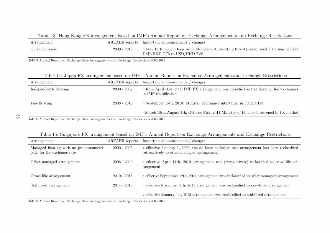
Table 13: Hong Kong FX arrangement based on IMF’s Annual Report on Exchange Arrangements and Exchange Restrictions

Arrangement AREAER reports Important announcements / changes

Currency board 2000 - 2016 ◦ May 18th, 2005: Hong Kong Monetary Authority (HKMA) established a trading band ofUSD/HKD 7.75 to USD/HKD 7.85

IMF’S Annual Report on Exchange Rate Arrangements and Exchange Restrictions 2000-2016

Table 14: Japan FX arrangement based on IMF’s Annual Report on Exchange Arrangements and Exchange Restrictions

Arrangement AREAER reports Important announcements / changes

Independently floating 2000 - 2007 ◦ from April 30st, 2008 IMF FX arrangement was classified as free floating due to changesin IMF classification

Free floating 2008 - 2016 ◦ September 15th, 2010: Ministry of Finance intervened in FX market

- March 18th, August 4th, October 31st, 2011 Ministry of Finance intervened in FX market

IMF’S Annual Report on Exchange Rate Arrangements and Exchange Restrictions 2000-2016

Table 15: Singapore FX arrangement based on IMF’s Annual Report on Exchange Arrangements and Exchange Restrictions

Arrangement AREAER reports Important announcements / changes

Managed floating with no pre-announcedpath for the exchange rate

2000 - 2005 ◦ effective January 1, 2006, the de facto exchange rate arrangement has been reclassifiedretroactively to other managed arrangement

Other managed arrangement 2006 - 2009 ◦ effective April 14th, 2010 arrangement was (retroactively) reclassified to crawl-like ar-rangement

Crawl-like arrangement 2010 - 2013 ◦ effective September 12th, 2011 arrangement was reclassified to other managed arrangement

Stabilized arrangement 2014 - 2016 ◦ effective November 9th, 2011 arrangement was reclassified to crawl-like arrangement

◦ effective January 1st, 2013 arrangement was reclassified to stabilized arrangement

IMF’S Annual Report on Exchange Rate Arrangements and Exchange Restrictions 2000-2016

36