Predicting environmental risk of transmission of leptospirosis

Predicting environmental risk of

transmission of leptospirosis

Thesis submitted in

accordance with the

requirements of the University

of Liverpool for the degree of

Doctor of Philosophy by

Gabriel Ghizzi Pedra

June 2019

Abstract

Predicting environmental risk of transmission of

leptospirosis

Gabriel Ghizzi Pedra

Leptospirosis is a zoonotic disease distributed worldwide, caused by contact with the

spirochete bacteria Leptospira. The bacteria are transmitted when animal and human

reservoirs come into contact with an environment contaminated with the urine of an infected

animal. The ecology of leptospirosis includes complex interactions between the

environmental reservoir, the animal reservoir, human infection and the bacteria. Most of the

knowledge built up about leptospirosis and human infection is related to medical

epidemiology and the animal reservoir. In this thesis, some of the main issues related to the

dynamics of Leptospira in the environment were explored and tools were developed to

improve understanding of the dynamics of the bacteria in the environment.

In order to improve parameter estimation related to the dynamics of the bacteria in the

environment, some major gaps were identified and techniques to fill those gaps improved.

The first technique developed was to improve animal abundance estimation using removal

methods. The improvement of the technique showed that animal abundance could be

estimated more accurately and precisely while also being robust to intrinsic variation. This

method will provide a more accurate estimation of the level of environmental contamination

by rats.

Although models that estimate bacterial survival in the environment exist, no models

specifically looked at the survivability of leptospires within the environment. Therefore, a

survival model was developed that could estimate survival rates of leptospires in microcosms

designed to replicate natural environments. The results provided very insightful results that

can help planning the duration and frequency of an environmental intervention.

Water has been shown to be very relevant for the transmission of human leptospirosis,

where rainfall has been associated with infections in endemic regions. The last two studies

developed here explored different hydrological techniques in order to produce fine scale

environmental risk maps which can be used in disease management.

The results obtained here demonstrated in particular the role of multidisciplinary

research. Here, the research produced an improvement of the knowledge in different areas

such as population ecology, microbiology, hydrology and public health.

Acknowledgements

Firstly, I would like to thank both my supervisors Mike Begon and Peter Diggle. Both of

you were essential in the development of my thesis. I will carry the things I have learnt

wherever I go. Thanks for your guidance and patience.

Secondly, I would like to thank Federico Costa who introduced me to the world of eco-

epidemiology, public health and leptospirosis in Salvador. Working in the field showed me

how essential it is to know your study subject and its importance in developing research

questions.

I would also like to thank Albert Ko for your advice and great discussions in Salvador to

define the course of my PhD. Also, I would like to thank everyone involved in the project

“Eco-epidemiology of urban leptospirosis”, the field work, data management, laboratory and

accounts team, without you all, nothing would be possible.

I would also like to thank CAPES for making the dream of studying a PhD possible, and

also, the University of Liverpool for providing the support and a great environment to work.

Thanks Allan McCarthy and Stephen Cornell for following the process of my thesis

development and providing great feedback.

Finally, I would like to thank all my friends who have made these the best four years of

my life.

Table of Contents

Chapter 1: Introduction ...................................................................................................... 1

1.1 Infectious diseases and environment ......................................................................... 1

1.2 Leptospirosis ............................................................................................................. 3

1.2.1 Epidemiology ...................................................................................................... 3

1.2.2 Reservoir hosts ................................................................................................... 5

1.2.3 Environment ....................................................................................................... 6

1.2.3.1 Leptospires in the environment.................................................................... 7

1.2.3.2 Environmental risk factors in human leptospirosis.......................................12

1.2.4 Geographical distribution of leptospirosis ..........................................................14

1.2.5 Conceptual model of the bacteria in the environment .......................................17

1.3 How hydrology can help infectious disease dynamics ...............................................20

1.4 Aims .........................................................................................................................21

1.5 Note on collaborative research and data collection ..................................................22

1.6 References ...............................................................................................................23

Chapter 2: A new approach to making multiple estimates of animal abundance using

removal methods ...............................................................................................................40

2.1 Introduction .............................................................................................................40

2.2 Materials and methods .............................................................................................42

2.2.1 The Borchers et al. (2002) method .....................................................................42

2.2.2 Pooled method ..................................................................................................44

2.2.3 Extension to non-constant probability of capture...............................................45

2.2.4 Simulation and validation of the model ..............................................................46

2.2.5 Application of the pooled method to Salvador data ...........................................48

2.2.6 Ethical statement ...............................................................................................50

2.3 Results......................................................................................................................50

2.3.1 Salvador data .....................................................................................................53

2.4 Discussion ................................................................................................................55

2.5 Acknowledgments ....................................................................................................58

2.6 Referrences ..............................................................................................................59

2.7 S1 APENDIX ..............................................................................................................65

2.8 S2APPENDIX .............................................................................................................66

Chapter 3: Survival analysis of Leptospira spp. in microcosms ............................................75

3.1 Introduction .............................................................................................................75

3.2 Materials and methods ............................................................................................ 78

3.2.1 Microcosms ....................................................................................................... 78

3.2.2 DNA extractions and bacteria quantification ...................................................... 79

3.2.3 Statistical modelling .......................................................................................... 80

3.2.3.1 Model ......................................................................................................... 80

3.2.3.2 Log-likelihood ............................................................................................. 82

3.2.3.3 Confidence intervals ................................................................................... 83

3.2.3.4 Checking assumptions................................................................................. 83

3.2.3.5 Model selection .......................................................................................... 84

3.3 Results ..................................................................................................................... 84

3.4 Discussion ................................................................................................................ 91

3.5 References ............................................................................................................... 95

Chapter 4: Hydrology and its implications to waterborne diseases ................................... 102

4.1 Introduction ........................................................................................................... 102

4.2 Material and methods ............................................................................................ 106

4.2.1 Flow accumulation .......................................................................................... 108

4.2.2 Population weighted accumulation .................................................................. 109

4.2.3 Water rurality .................................................................................................. 111

4.2.4 Topographic Wetness Index (TWI) ................................................................... 111

4.3 Model output ......................................................................................................... 112

4.4 Application to Salvador city .................................................................................... 115

4.5 Discussion .............................................................................................................. 124

4.6 References ............................................................................................................. 128

Chapter 5: 14 years of leptospirosis surveillance in Salvador city, Brazil: spatial distribution

of leptospirosis cases and its relationship with hydrology ................................................ 135

5.1 Introduction ........................................................................................................... 135

5.2 Material and methods ............................................................................................ 138

5.2.1 Study area ....................................................................................................... 138

5.2.2 Data collection and case definition .................................................................. 138

5.2.3 Hydrological data............................................................................................. 139

5.3 Statistical analysis .................................................................................................. 140

5.3.1 Non-spatial model ........................................................................................... 141

5.3.2 Empirical variogram ......................................................................................... 142

5.3.3 Geostatistical model ........................................................................................ 143

5.3.4 Model validation ............................................................................................. 145

5.3.5 Identification of areas with high risk of leptospirosis transmission ................... 145

5.3.6 Risk of having at least one case of human leptospirosis ....................................146

5.4 Results....................................................................................................................146

5.5 Discussion ..............................................................................................................154

5.6 References .............................................................................................................160

Chapter 6: General discussion ..........................................................................................167

6.1 The value of methodological advances ...................................................................170

6.2 Post script: Two years of work in the community of Pau da Lima and how the results

of this thesis can help the community ..........................................................................173

6.3 References .............................................................................................................176

1

Chapter 1: Introduction

1.1 Infectious diseases and environment

The global population is growing fast. In the past 50 years, city-dwelling has

increased exponentially and now more than 50% of the population are living in

urban centres. Unfortunately, access to safe drinking water and sanitation has not

followed the rapid urbanisation and the number of inadequate settlements has

increased: 881 million people were living in urban slums in 2014 (Moreno et al.,

2016). In addition, 32% of the global population still lack adequate sanitation and it

is estimated that half of the world’s population will be living in tropical environments

by 2050, which is the region with the highest incidence of infectious diseases on the

globe (Guernier, Hochberg and Guégan, 2004; Hemingway, 2014).

As a consequence of population growth there has been an increase in the

number of infectious diseases, mainly in urban areas. Pathogens are emerging or

re-emerging, representing a threat to people’s life and wellbeing. This might be

caused by changes in the environment, such as the expansion of urban areas into

natural environments, which increases exposure to pathogens and changes the

dynamics of infectious diseases. Zika, Ebola, SARS and H1N1 are examples of

emerging infectious diseases that have caused a significant impact due to change in

the pathogen dynamics and environment in the last decade. In 2012, environmental

factors could be identified as the cause of 23% of all deaths reported globally,

mostly in low and middle-income countries hold most of it (Prüss-Ustün et al., 2016).

2

The role of the environment in the dynamics of infectious disease transmission is

important both because it may be involved in the life cycle of a pathogen and/or may

be one of the routes of transmission. Annual variations in mean precipitation, and

annual temperatures, have been shown to be predictors of pathogens species

distributions based on a global analysis (Guernier, Hochberg and Guégan, 2004).

The main taxa affected by these patterns have an ‘external’ stage, such as

helminths, which requires a free-living stage to complete its life cycle. Besides

explaining global distribution of the pathogens, rainfall and temperature have been

reported as a risk factor for humans for many infectious diseases. Malaria, cholera,

dengue and leptospirosis are a few of the examples of diseases that have reported

this association.

Climate change predictions are showing that temperature and precipitation are

rising globally and that tropical environments will expand towards temperate

environments. This expansion can affect the distribution of the many infectious

diseases that are related to temperature and rainfall and occur in the tropics.

Therefore, together with rapid urbanisation and population growth, climate change

will change the distribution of infectious diseases by increasing its distribution range

towards temperate climates. Understanding the role of the environment in the

transmission and life cycle of pathogens can be relevant to inform health authorities

in the public management of resources to reduce transmission and improve people’s

life and wellbeing.

A disease that have been changing its epidemiology due to urbanisation in the

last 50 years is leptospirosis. Leptospirosis used to affect mostly miners and rice

plantation workers in rural areas. However, the rapid urbanisation and the growth of

inadequate settlements have changed its epidemiology and, nowadays, it is

associated with low-income communities and can be considered an occupational

disease. The disease is worldwide in its distribution but the places with the highest

3

incidence are tropical countries. The next sections will provide an overview of

leptospirosis, how the environment is involved in the life cycle of the pathogen, and

in its disease transmission.

1.2 Leptospirosis

1.2.1 Epidemiology

Leptospirosis is a zoonotic disease distributed worldwide and caused by contact

with the spirochete bacteria Leptospira of which there are over 200 serovars

described. It was originally considered mostly a rural disease, but rapid urbanization

and other environmental changes have led to changes in the dynamics of the

bacteria. In 2003 the World Health Organization (WHO) classified leptospirosis as a

neglected disease and found it to be more frequent in developing countries with

poor sanitation conditions (WHO, 2003b). It is estimated that approximately

1,000,000 cases and 59,000 deaths are caused by disease around the world each

year (Costa, Hagan, et al., 2015).

Many animals are considered to be reservoir hosts in which the infection can be

asymptomatic and pathogenic Leptospira are shed through the urine during the

entire lifetime of the host (Babudieri, 1958; Thiermann, 1981; Faine et al., 1999).

Nearly all mammals can carry the bacteria (Thiermann, 1977; Bunnell et al., 2000;

Levett, 2001), but the natural reservoirs of bacteria threatening humans are often

rodents (Faine et al., 1999). The bacteria colonize the kidneys of its hosts and are

eliminated in the urine from infected animals and can persist in the environment,

potentially, for long periods (between one week and a few months) (Faine et al.,

1999; Trueba et al., 2004b). Humans may be infected through direct contact with an

infected animal or through an environment contaminated by urine of those animals.

4

Infection might occur through penetration of damaged skin or mucous surfaces

(Faine et al., 1999). There is no human to human infection as the concentration of

the bacteria shed by humans is too low for them to be considered a reservoir (WHO,

2003b).

Infections in humans by Leptospira do not always result in clinical symptoms; it

can be asymptomatic or the disease can be considered biphasic with an acute

and/or a severe phase. Acute leptospirosis symptoms can include fever, severe

headache, myalgia, nausea, vomiting, chills, malaise and conjunctival hyperaemia

(Fraga et al., 2015). In severe cases, the clinical symptoms can be jaundice,

myocarditis, meningitis, renal failure, lethal pulmonary haemorrhage and multiorgan

failure. Severe cases can be a result of a single illness or a second phase of the

acute phase. Renal failure (Weil’s disease) and pulmonary haemorrhage cause

fatality in 30% and 50% of cases, respectively (Faine et al., 1999; World Health

Organization, 2003). Leptospirosis is often misdiagnosed due the similarity that

acute symptoms have with other diseases, such as dengue and typhoid fever, which

results in an underestimated number of cases (WHO, 2003b; Marchiori et al., 2011;

Fraga et al., 2015). In addition, laboratory diagnose is complex, expensive and time

consuming because it involves Leptospira culture, PCR techniques, IgM-ELISA and

microscopic agglutination test (MAT) depending which infection phase patients are

in (Faine et al., 1999; Levett, 2001; Marchiori et al., 2011; Fraga et al., 2015).

There are varying patterns of human infection and those patterns depend on the

ecological setting. In rural settings, the infections are associated with agricultural

and livestock areas and there are peaks of transmission during rainy seasons (Faine

et al., 1999; Bharti et al., 2003; McBride et al., 2005). In urban areas the infections

are associated with poor sanitation, overcrowding and poverty in developing

countries (A I Ko et al., 1999; Levett, 2001; Vanasco et al., 2008). In developed

5

countries, outdoor recreational exposure and international travel have been

associated with the infection (Lau et al., 2010a).

1.2.2 Reservoir hosts

Rodents have been found to be the main reservoir of the bacteria despite the

bacteria also occurring in other mammal species. In urban areas, rats carry the

bacteria with varied prevalence. High prevalence of infected rats has been reported

in Baltimore, USA for example, where 65% of rats sampled were infected with the

bacteria (Easterbrook et al., 2007). In Salvador, Brazil, the prevalence was even

higher with 80% of the animals infected (de Faria et al., 2008). On the other hand,

only 11% of the animals were infected in Vancouver, Canada (Himsworth et al.,

2013). Rats are the main source of human leptospirosis in urban areas. Most of the

human cases come from serovars that is found in species of Rattus (Levett, 2001).

Other rodent species can also carry the bacteria and serve as a reservoir. For

example house mice, voles, shrews, muskrats and coypus were also found to be

infected (Michel et al., 2001; Adler et al., 2002; Turk et al., 2003; Aviat et al., 2009).

Other mammals can also be a reservoir for leptospirosis, such as livestock animals

and wild animals. In livestock farming, infected animals can be a risk factor for

farmers and butchers in developing countries (Levett, 2001). Cattle, sheep, pigs and

goats are farming animals that have been reported as carrying leptospirosis (Levett,

2001; Dorjee et al., 2008; Brown et al., 2011; Suepaul et al., 2011; dos Santos et al.,

2012; Martins and Lilenbaum, 2013). Wildlife populations have also been reported

as reservoirs. In Pantanal, Brazil, 40% of the animals of four wild mammals species

were positive for the bacteria (Vieira et al., 2016), whereas in Africa, birds and

reptiles were found positive (Jobbins and Alexander, 2015). Finally, marsupials, bats

and rodents have been found carrying the bacteria in the Amazon (Bunnell et al.,

2000).

6

Some animals are reservoir for one serovar and susceptible for others. For

example, canine populations are reservoirs for the serovar Canicola but are very

susceptible to others serovars (Goarant, 2016). Similarly, for cattle, the common

serovar is Hardjo and for pigs it is Australis. These associations can be related to

evolution and adaptation of the parasite which is advantageous to a successful

establishment in the host population. Other associations are between rats and

serogroup Icterohaemorrhagiae; and mice and serogup Ballum (Goarant, 2016).

These associations have helped health authorities to identify the source of human

leptospirosis in particular cases.

1.2.3 Environment

Pathogenic leptospires are not able to reproduce in the environment but are able

to survive from days to months, as elaborated below. Animal reservoirs and humans

can be infected if in contact with an environment contaminated with the urine of an

infected animal. However, the role of the environment seems to be more relevant in

human infections than in the animal reservoir. Minter et al. (2017) modelled the

routes of transmission between animal reservoirs and identified that 17% of the

youngest captured animals had leptospirosis. Their results indicate that transmission

occurs before the animals leave their nests and suggest vertical transmission as one

of the routes of transmission together with the environment transmission. In

humans, the environment can be considered its primary source of infection where

environmental variables are one of the main risk factors related to the disease (see

section 1.2.3.2).

The search for the bacteria in the environment started when the epidemiology of

the disease revealed that the infections were associated with a patient’s occupation

and were first described in soldiers, miners, and sewer worker and rice planters, all

7

in wet conditions (Faine, 1982; Katz, Manea and Sasaki, 1991; Faine et al., 1999).

Some epidemics were found in sugar cane cutters, rice harvesters and stable hands

in cattle stables (Faine et al., 1999). These findings boosted studies to search for

the presence and distribution of the bacteria in the environment, such as water and

soil samples, where the infections occurred.

Baker and Baker (1970) were one of the pioneers to demonstrate the

pathogenicity of water and wet soil in transmitting leptospirosis. Firstly, they

identified water and soil samples that were positive for pathogenic leptospires, then

inoculated them in hamsters and observed the survival of the animals.

Approximately 30% of the deaths could be attributed to leptospirosis and the

estimated survival time was around nine days. On the other hand, Henry and

Johnson (1978) isolated leptospires from water and soil samples, but they were from

the Biflexa serogroup and they could not infect any of the experimental animals,

supporting the believe that this serogroup is nonpathogenic. The following sections

will explore how the environment is related with the bacteria itself in terms of

persistence and occurrence; and how it is related to the transmission of human

leptospirosis.

1.2.3.1 Leptospires in the environment

The search for the bacteria in the environment was inspired from

epidemiological studies as previously mentioned. Here, a literature review was

performed in 2016 and was intended to find and describe the occurrence of the

bacteria in the environment. The literature review was performed using Web of

Knowledge and the words used were: “Leptospira”; and “Leptospira*Environment”.

The criteria of inclusion were studies where the presence of the bacteria was

evaluated in environmental samples, such as water and soil. In total, 21 studies

8

were selected and information was collected in each case such as location, setting

(urban or rural), year, species group (pathogenic or saprophytic), type of sample

(rodent, soil or water), total number of samples, proportion of positive samples and

method used (culture, PCR or qPCR). The results are presented in Table 1.1.

9

Table 1.1: Results of the presence of Leptospira spp. obtained from environmental studies. NA= not available.Year Area Location Country Species Method Authors (year)

Positive Total % Positive Total % Positive Total % % moisture

1973 rural Illinois USA both NA NA NA 56 101 55.4 NA NA NA NA culture Tripathy & Hanson 1973

1978 natural reserve lake Minnesota (USA) saprophytic NA NA NA 83 126 65.9 15 20 75.0 6.8-86.5 culture Henry & Johnson 1978

1978 natural reserve stream Minnesota (USA) saprophytic NA NA NA 30 30 100.0 NA NA NA NA culture Henry & Johnson 1978

1978 natural reserve bog Minnesota (USA) saprophytic NA NA NA 2 35 5.7 15 34 44.1 27-75 culture Henry & Johnson 1978

1978 natural reserve spring water/soil Minnesota (USA) saprophytic NA NA NA 8 28 28.6 22 37 59.5 25-82 culture Henry & Johnson 1978

1994 NA NA China pathogenic NA NA NA 3 140 2.1 5 102 4.9 NA culture Yang et al . 1994

2006 urban market area Belem (Peru) pathogenic NA NA NA 53 78 67.9 NA NA NA NA qPCR Ganoza et al . 2006

2006 urban living area Belem (Peru) pathogenic NA NA NA 38 114 33.3 NA NA NA NA qPCR Ganoza et al . 2006

2006 rural rural area Padrecocha (Peru) pathogenic NA NA NA 60 236 25.4 NA NA NA NA qPCR Ganoza et al . 2006

2009 rural camps Malasya both NA NA NA 15 144 10.4 15 145 10.3 NA culture/PCR/MAT Ridzlan et al . 2009

2009 urban multiple cities France pathogenic 38 516 7.4 114 151 75.5 NA NA NA NA PCR Aviat et al . 2009

2009 rural areas Guilan province Iran both NA NA NA 40 222 18.0 NA NA NA NA culture Issazadeh et al . 2009

2010 urban Rio de Janeiro Brazil both NA NA NA 3 100 3.0 NA NA NA NA Multiplex/PCR Vital-Brazil et al . 2010

2011 coastal streams NA Hawai pathogenic NA NA NA 87 88 98.9 NA NA NA NA qPCR Viau & Boehn 2011

2013 urban Metro Manila Philipines both NA NA NA 8 39 20.5 NA NA NA NA culture Saito et al . 2013

2013 rural Nueva Ecija Philipines both NA NA NA 13 18 72.2 3 3 100.0 NA culture Saito et al . 2013

2013 urban Fukuoka Japan both NA NA NA 10 16 62.5 3 12 25.0 NA culture Saito et al . 2013

2013 rice crop Tonekabon Iran saprophytic NA NA NA 35 67 52.2 16 36 44.4 NA culture Yassouri et al . 2013

2013 urban multiple sites Malasya both NA NA NA 28 121 23.1 7 30 23.3 NA culture Benacer et al . 2013

2013 pig farm Monteria Colombia pathogenic NA NA NA 2 54 3.7 NA NA NA NA cultue/PCR Calderon et al. 2013

2014 coast Leyte province Philipines pathogenic NA NA NA NA NA NA 11 23 47.8 NA culture Saito et al . 2014

2014 urban/flooding Lublin Poland both NA NA NA 2 40 5.0 0 40 0.0 NA PCR Wójcik-Fatla et al . 2014

2014 urban/non flooding Lublin Poland both NA NA NA 0 64 0.0 0 68 0.0 NA PCR Wójcik-Fatla et al . 2014

2014 rice crop Tonekabon Iran pathogenic NA NA NA 29 67 43.3 9 36 25.0 NA culture Yassouri et al . 2014

2014 rural village Los Rios Chile pathogenic NA NA NA 27 213 12.7 NA NA NA NA PCR Muñoz-Zanzi et al . 2014

2014 farms Los Rios Chile pathogenic NA NA NA 50 357 14.0 NA NA NA NA PCR Muñoz-Zanzi et al . 2014

2014 island St kitts Caribe pathogenic NA NA NA 8 44 18.2 NA NA NA NA qPCR Rawlins et al . 2014

2015 urban Sedayu district Indonesia pathogenic 6 31 19.4 13 32 40.6 13 36 36.1 NA qPCR Sumanta et al. 2015

2015 urban Bantul district Indonesia pathogenic 10 36 27.8 29 52 55.8 38 61 62.3 NA qPCR Sumanta et al. 2015

2015 urban Sewon district Indonesia pathogenic 9 32 28.1 9 35 25.7 13 53 24.5 NA qPCR Sumanta et al. 2015

2012 urban Andaman Island India pathogenic NA NA NA 11 113 9.7 NA NA NA NA PCR Lall et al . 2016

2012 urban Andaman Island India nonpathogenic NA NA NA 50 113 44.2 NA NA NA NA PCR Lall et al . 2016

2012 rural Andaman Island India pathogenic NA NA NA 9 133 6.8 NA NA NA NA PCR Lall et al . 2016

2012 rural Andaman Island India nonpathogenic NA NA NA 58 133 43.6 NA NA NA NA PCR Lall et al . 2016

2014 urban Andaman Island India pathogenic NA NA NA 15 56 26.8 NA NA NA NA PCR Kumar et al . 2015

2014 rural Andaman Island India pathogenic NA NA NA 19 86 22.1 NA NA NA NA PCR Kumar et al . 2015

Water SoilRodents

10

The presence of Leptospira in the environment varies between locations, and

consequently the proportion of positive samples varied in each study. It was

observed that Leptospira are able to survive in alkaline soil, mud, swamps, streams

and rivers, organs and tissues of live and dead animals or dilute milk (Faine et al.,

1999). Overall, water and soil samples were taken from streams, nature reserves,

rice crops, farms, rural areas, urban areas, flooding and coastal areas. The locations

varied from temperate countries such as the USA, France and Poland to tropical

countries such as the Philippines, Indonesia and the Caribbean. Saprophytic and

pathogenic bacteria were examined together or separately, and the technique used

to detect the bacteria varied from culture methods to DNA amplification methods

such as qPCR.

There was a gap of approximately 20 years from the first studies that evaluated

the presence of the bacteria in water and sample soils until the next study was

published. This could be a result of the development of more sophisticated

techniques to detect Leptospira in the environment. Despite culture techniques

being considered gold standard methods, they are expensive, time consuming and

the media used are not specific for leptospirosis which increases the number of false

negatives. When DNA techniques became more accessible, studies that explored

the occurrence of leptospires in the environment started appearing again. The

renewal of interest may also have happened because leptospirosis has changed its

epidemiology. The incidence of human leptospirosis increased and WHO included

leptospirosis as a neglected disease of general concern in 2003. This raised

awareness of leptospirosis and studies started to explore and understand patterns

of infection and how transmission occurs.

Tripathy and Hanson (1973) were the pioneers who isolated pathogenic bacteria

from water samples in an agricultural center in Illinoi. They were followed by

11

Alexander et al. (1975) who isolated leptospires from surface water and wet soil in

the Malaysian jungles. They found a variety of serovars that was consistent with the

ones identified from soldiers who had leptospirosis at the time. Henry and Johnson

(1978) found over 92% of positive water and soil samples in Minnesota when the

average temperature was 25°C. In addition, the proportion of positive sample was

higher for soil samples than water where the moisture content of the soil was greater

than 65%.

In general, the proportion of positive water samples varied from 3% in an urban

area of Rio de Janeiro, Brazil (Vital-Brazil et al., 2010), to 67% and 75% in an urban

area in Peru and France respectively (Ganoza et al., 2006; Aviat et al., 2009). In

rural areas, this varied from 3.7% in a pig farm in Colombia (Calderón et al., 2014)

to 100% in a nature reserve in Minnesota (Henry and Johnson, 1978). The bacteria

were also able to survive in seawaters. Saito et al. (2014) observed that the bacteria

that comes from soil to the seawater, survived for four days in seawater whereas the

bacteria inoculated straight in seawater survived for three days only. Their results

suggest that the soil increased the chance of the bacteria surviving in seawater.

Fewer studies have evaluated the presence of the bacteria in the soil, and only

one study looked at how the moisture of the soil is related with positive samples.

The proportion of positive soil samples in urban areas varied from 0% in Poland

(Wójcik-Fatla et al., 2014) to 62% in Bantul district, Indonesia (Sumanta et al., 2015)

,whereas, in rural areas, it varied from 10% in rural camps in Malaysia (Ridzlan et

al., 2010) to 75% in a stream in Minnesota (Henry and Johnson, 1978). Henry and

Johnson (1978) were the only investigators who observed that soils with higher

moisture had the highest proportion of positive samples.

Another factor that affects the survival of leptospires in the environment is pH.

Okazaki and Ringen (1957) observed that the bacteria survived in the environment

with pH ranging from 6 to 8.4. Similarly, Diesch et al. (1969) observed that the

12

bacteria survived in creek water at a pH ranging from 6.9 to 8.7. None of these

studies has quantified the survival of the bacteria in the environment, and until now,

the rate at which the cells died in the environment is unknown.

The results on the occurrence of pathogenic bacteria in soil and water samples

indicates that these environments can be considered a reservoir for the bacteria.

The association between outbreaks of leptospirosis and floods and/or heavy rain

(see section 1.2.3.2) could plausibly be a result of the presence of the bacteria in the

environment that increases exposure to the disease. Most of the research, if not all,

has focused on finding the bacteria in different environments. However,

understanding the survival and transportation of the bacteria in the environment can

be crucial to understanding its distribution and how the environmental risk of

transmission of leptospirosis can be estimated.

1.2.3.2 Environmental risk factors in human leptospirosis

Human leptospirosis was previously considered an occupational and rural

disease, as mentioned, where the first description of cases came from farmers,

soldiers, miners and rice plantations. Baker (1965) described a leptospirosis

outbreak between soldiers in Malaysia and identified that most of the individuals had

been to the forest a drunk water that might have been contaminated. In Britain, most

of the cases reported between 1933-48 were farmers/fisher workers, coal miners,

sewer workers and soldiers (Waitkins, 1986). Additionally to the importance of

occupation, recreational activities were also related to occurrence of infection,

whereby canoeists were reported having leptospirosis (Waitkins, 1986). Nowadays,

human leptospirosis cases have increased and it is also frequently reported in urban

environments. However, environmental risk factors are reported in both urban and

rural environments. From a combination of epidemiological, cohort (transversal and

13

longitudinal) and case-control studies, risk factors have been identified and related

with socioeconomics and environmental characteristics (A I Ko et al., 1999;

Barcellos and Sabroza, 2001a; Sarkar et al., 2002; Maciel et al., 2008; Reis et al.,

2008; Ko, Goarant and Picardeau, 2009; Oliveira et al., 2009; Hagan et al., 2016).

Lower levels of income and education are the most important socioeconomic

characteristics affecting the infection (Barcellos and Sabroza, 2001a; Reis et al.,

2008; Oliveira et al., 2009). Environmental risk factors varied and included variables

such as contact with mud, elevation, flooding, open sewage and litter less than ten

meters from residences. Such links have been found with asymptomatic infection

and with severe cases of the disease (A I Ko et al., 1999; Sarkar et al., 2002; Reis et

al., 2008; Oliveira et al., 2009; Hagan et al., 2016).

Hagan et al. (2016), in a four year prospective study, identified that leptospirosis

transmission in a urban slum in Salvador, Brazil, was associated with poverty,

geography and climate. Illiteracy, the level of rat infestation, contact with mud, and

elevation were all related with the infections throughout the four years follow-up.

Distance to an open sewer and household income were related to primary and

secondary infections in the same urban slum, suggesting that environmental setting

and behaviour contributes to exposure to Leptospira (Felzemburgh et al., 2014a).

Similarly, in a urban slum in Rio de Janeiro, Brazil, the environmental risk factors

associated with leptospirosis were solid waste accumulation and coverage, flood

risk areas, proximity to sewer and proximity to rainwater drainage (Barcellos and

Sabroza, 2001a; Sarkar et al., 2002; Reis et al., 2008). However, these

environmental risk factors are imperfect proxies for the presence of the bacteria and

do not represent the intensity of environmental contamination. Flooding and heavy

rain are also associated with infections in endemic and non-endemic regions. They

are responsible for outbreaks and for the seasonality on the number of cases

observed in endemic regions. Ko et al. (1999) observed that rainfall was responsible

14

to an increase on the number of cases in Salvador, Brazil where the maximum

number of infections occurred two weeks after the heaviest rainfall of the year. In

Malaysia, leptospirosis is endemic, and flooding have been associated with human

cases (Garba, Bahaman, Khairani Bejo, et al., 2017). Studies have shown this

relationship with between rainfall and leptospirosis cases in another endemic

regions such as Thailand and tropical islands (Goarant et al., 2009a; Desvars et al.,

2011a; Chadsuthi et al., 2012a).

An outbreak in Philippines in 2009 occurred after a flooding event where 178

people died after a typhon caused a major flood in the city of Metro Manila

(Amilasan et al., 2012a). Similarly, unusual epidemics of leptospirosis and

melioidosis occurred after a typhon reached Taiwan on the same year (Su, Chan

and Chang, 2011). Furthermore, outbreaks of leptospirosis, also have been

associated with rainfall in many other countries such as Australia (Smythe et al.,

2002), Brazil (Barcellos and Sabroza, 2001a; Blanco and Romero, 2015), France

(Socolovschi et al., 2011), Guyana (Dechet et al., 2012), Hawaii (Gaynor et al.,

2007), Honduras (Naranjo et al., 2008), India (Sehgal, Sugunan and Vijayachari,

2002; Jena, Mohanty and Devadasan, 2004; Pappachan, Sheela and Aravindan,

2004), Malaysia (Garba, Bahaman, Khairani-Bejo, et al., 2017), Nicaragua (Zaki and

Shieh, 1996; Schneider et al., 2012), the Philippines (Amilasan et al., 2012b; SUMI

et al., 2017), Thailand (Chadsuthi et al., 2012b), United States (Stern et al., 2010).

1.2.4 Geographical distribution of leptospirosis

Costa et al. (2015) estimated global morbidity and mortality of leptospirosis

where the estimations shown that the regions with the highest incidence of the

disease are Southeast Asia, Oceania and Caribbean (Figure1.1). Those areas also

have the highest annual average rainfall on the globe (Fick and Hijmans, 2017) as

15

shown in Figure 1.2, from which it is clear that water is playing an important role in

human infection – another reason for environmental studies indicating

environmental levels of contamination are important both to understand and to

predict the environmental risk of infection.

Figure 1.1: Figure extracted from Costa et al. (2015) showing the estimated morbidity of leptospirosis based on systematic literature review. The colour gradient represents number of cases per 100,000 population where white represent cases from 0 to 3, yellow from 7 to 10, orange from 20 to 25 and red over 100.

Figure 1.2: Annual average of precipitation (mm) data between 1960-1990 obtained from WorldClim repository - http://worldclim.org/version2 (Fick and Hijmans, 2017). Map author: Gabriel Ghizzi Pedra.

http://worldclim.org/version2

16

Human leptospirosis does not only vary globally. Distributions of cases within a

city or a country are also found to be geographically clustered. For example, at a city

level, Gutiérrez & Martínez-Vega (2018) identified six clusters of incidence of

leptospirosis in Colombia, South America, and identified that anomalous rainfall

were associated with elevated number of cases. There was evidence that

agriculture was a common factor in municipalities that have higher incidence of

leptospirosis (García-Ramírez et al., 2015). At a district level, an uneven distribution

of leptospirosis cases was observed in New Caledonia (Goarant et al., 2009a),

Futuna, south pacific (Massenet et al., 2015), Republic of Serbia (Svirčev et al.,

2009), Thailand (Suwanpakdee et al., 2015), Siri Lanka (Robertson, Nelson and

Stephen, 2012), Mexico (Sánchez-Montes et al., 2015), American Samoa (Lau et

al., 2012), Nicaragua (Schneider et al., 2012), China (Dhewantara et al., 2018) and

Trinidad (Vega-Corredor and Opadeyi, 2014). Even at a very small scale,

geographical variation have been observed. In Brazil, Hagan et al. (2016) observed

geographical variation on the risk of infection at a very small scale, within a low-

income community in Salvador, Brazil.

All those studies have found association with environmental variables, such as

rainfall and flooding, which also supports the idea that water is an important risk

factor at many scales. Furthermore, Gracie et al. (2014) evaluated the effect of

different risk factors on the incidence of leptospirosis at different scales. They found

an association between the proportion of areas prone to flood and leptospirosis at a

local scale, whereas the percentage of densely urbanized areas and the number of

households in slums were associated at a regional level. The use of geographically

distributed data helps to identify high risk areas that can further be used to target

actions to control and prevent leptospirosis incidence.

17

1.2.5 Conceptual model of the bacteria in the environment

To understand the mechanisms of disease transmission, it is necessary to know

the life cycle of the pathogen and the determinants of its occurrence. There is still a

lack of information on the determinants of bacterial occurrence and transport in the

environment. We have shown the role of the environment in human leptospirosis as

well as in its reservoir host, but knowledge of what happen with the bacteria in the

environment is still very basic and is growing. In this section, a conceptual model

that represents the dynamics of the bacteria in the environment is proposed and this

thesis will explore key compartments of this conceptual model.

Based on what has been shown here and further discussion with experts on

leptospirosis, a conceptual model was developed. This conceptual model is a

simplification of the complex interaction between the bacteria and the environment

and it is shown in Figure 1.3.

Figure 1.3: Conceptual model representing the dynamics of the bacteria in the environment. The boxes represent the location where the bacteria occur, called compartments. Blue arrows represent movements between compartments. Red and black arrows are the way the bacteria leave the system – by mortality (dark) or human infection (red). Lambda represents a reservoir of the bacteria external to the system, often a population of rats.

18

The bacteria get into the environment through shedding from an animal

reservoir, represented by lambda. This quantity depends on the reservoir’s

abundance and the shedding rate, which will indicate the level of local

contamination. Leptospirosis shedding rate varies depending on the animal

reservoir. Rats, Rattus norvegicus, shed approximately 5.7 × 106 cells/ml of urine

whereas large mammals such as cattle shed less, 1.7x105 cells/ml (Barragan et al.,

2017). Costa et al. (2015) estimated that a population of 82 rats would shed daily

more than 9.1 x 1010 leptospires. However, the population size of the reservoir often

remains unknown and in studies that attempt to incorporate abundance, this has

either been assumed to be the total number of animals trapped (Costa, Wunder, et

al., 2015) or relative abundance has been used (Himsworth et al., 2013). These

attempts do not represent absolute abundance of a population and therefore the

level of contamination cannot be properly estimated. CHAPTER 2 of this thesis will

demonstrate a new method to estimate absolute abundance, applicable especially

to rats in urban environments, and show the difficulties of current techniques on

estimating animal abundance.

The central assumption of the model in Figure 1.3 is that there are three

environmental states where the bacteria is present: soil surface, soil sub-surface

and water bodies. Saito et al. (2013), for example, observed Leptospira at 3cm

depth after three drought days at a location that was a dried rain puddle previously.

In addition, the same place was positive for Leptospira five months later. This

observation indicates a role for the sub-surface as a reservoir of the bacteria in the

environment, but there is still very little information about this environmental state.

The bacteria leave each state based on a survival rate or human infection

represented by the black and red arrows, respectively, in the figure. Neither the

quantitative nor the qualitative nature of the survival curve of the bacteria is known,

and in a collaboration between the University of Liverpool and Yale University,

19

microcosms experiments were developed to estimate the survival rate of the

bacteria in different environments such as spring water, soil, mud and sewage. The

results of these experiments are shown on CHAPTER 3 where a statistical survival

model was developed.

It is evident that water plays an important role in leptospirosis transmission,

since most of the environmental risk factors are water related variables. There are

peaks in the number of cases every year in endemic areas and they have been

associated with rainfall. In addition, outbreaks are reported after extreme weather

events, such as typhoons, El Niño events and heavy rainfall. Therefore, the

mechanisms behind bacteria transportation between the compartments in the

environment are driven by hydrology, where runoff carries the bacteria from soil to a

water body and flooding will do the opposite (blue arrows). The survival of the

bacteria is very short at the soil surface as the bacteria is exposed to ultraviolet

radiation and dehydration. Hence, there is no movement from the surface to the

water body and the bacteria pass to the sub-surface via diffusion.

Hydrology has not been explored extensively in leptospirosis studies. An

investigation by Vega-Corredor & Opadeyi (2014) was the only study that looked at

how hydrology can be associated with human leptospirosis. Their research was

based in Trinidad and Tobago, two islands in the Caribbean region and they

collected information on leptospirosis cases at a community level (~250

communities). It found that areas that are more likely to be flooded are the ones

where more cases of leptospirosis were observed. CHAPTER 4 will develop

methodologies, exploring how it is possible to use hydrology to create more

informative maps related to bacteria contamination, and in CHAPTER 5 the

association between these maps will be validated with surveillance data on

leptospirosis in Salvador, Brazil.

20

1.3 How hydrology can help infectious disease

dynamics

As a basic definition, hydrology is a discipline focused on the movement,

distribution and quality of water. Some of the areas within Hydrology are interested

in water flow, which can be looked at different scales. The process behind water

flow can involve precipitation, topography, evapotranspiration, soil saturation and

groundwater movement, all of which will influence the amount of water flowing or

accumulating in certain areas. However, water flow will primarily depend on the rain

that falls on the ground and the amount of that rain that becomes runoff. Two

different classes of mathematical models have been developed to understand the

water flow – lumped and distributed models. Lumped models work at a catchment

level and do not include finer-scale spatial variation, whereas distributed models

work at a fine scale and therefore rely on the spatial resolution of the data captured.

Waterborne diseases, as the name suggests, rely on water for pathogen

transportation and/or infection. They are called waterborne because the main route

of transmission occurs through water. Examples of waterborne diseases include the

historical cholera that is estimated to have killed over one million people in Europe in

the 19th century, typhoid fever, diarrheal diseases, schistosomiasis, dengue,

cryptosporidiosis, SARS (Severe Acute Respiratory Syndrome) and leptospirosis.

Hydrological models have been integrated with dynamic modelling of waterborne

diseases. The assumption behind the use of hydrology is that water can mobilize

pathogens, hence, modelling water flow can indicate the routes of pathogen

contamination and distribution. Medema & Schijven (2001) modelled the

transportation of Cryptosporidium and Giardia in the Netherlands to identify the

21

origin of contamination. It was observed that most of Cryptosporidium contamination

came from wastewater treatment plants, whereas, Giardia had most of

contamination coming from untreated wastewater discharge and sewer overflow.

Pathogen load were also addressed by Ferguson et al. (2007) and Mahajan et al.

(2014) where their aim was to identify the sources of contamination.

Additionally, the assumption of pathogen transportation was incorporated by

using river networks. Bertuzzo et al. (2008) integrated river pathways to model an

outbreak of cholera in South Africa in 2000. They were able to show how the

predictive power of the tool and how the river pathways played an important role in

controlling the direction of the infections. Subsequently, Mari et al. (2012) showed

that long-range human movement was able to explain the unexplained inter-

catchment movement of the pathogen. For schistosomiasis, the hydrological

transport was integrated in the vector compartment. Channel flows were key to

predict infection intensity and in periods of absence of flow, the risk was significantly

reduced (Remais, Liang and Spear, 2008). The ephemerality of rivers we also

shown to be associated with schistosomiasis cases in West Africa (Perez-Saez et

al., 2017).

Hydrological models can also help predict abundance of vectors. Shaman et al.

(2002) used a dynamic hydrological model to predict mosquitoes’ abundance. They

used a combination of historical meteorological data, topography, soil and

vegetation information to produce wetness map of the surface. From that, they

identified potential swamp and fresh water hence and predicted mosquitoes’

abundance.

1.4 Aims

22

In summary, the ecology of leptospirosis includes complex interactions between

the environmental reservoir, the animal reservoir, human infection and the bacteria.

All those compartments have an important role to play in transmission, but most of

the knowledge built up about leptospirosis and human infection is related to

epidemiology and the animal reservoir. Therefore, the main aim of this thesis is to

develop new tools related to the dynamics of the bacteria in the environment. It is

hoped that the tools developed here will facilitate environmental research and

contribute to understanding the main environmental drivers of human leptospirosis.

Furthermore, this thesis aims to enhance the application of hydrology in

infectious disease dynamics by exploring hydrological techniques and associating

results with disease outcomes. Understanding these relationships will help to

produce fine scale environmental risk maps, which can be used in disease

management.

1.5 Note on collaborative research and data

collection

This project is part of a multidisciplinary project with three institutions involved,

Oswaldo Cruz Foundation (Fiocruz, Brazil), University of Liverpool (UK) and Yale

University (USA). The project is called “Eco-epidemiology of urban leptospirosis”

and the main aim is to determine the main drivers of human infection. There are

data collection in all compartments related to the infection, reservoir, humans and

environment. Not all data used in this thesis was collected by the author. The data

23

collection on rodents were performed by a team, including the author, based in

Salvador, Brazil, where Fiocruz was responsible for the data collection and quality

control. Laboratory analysis from chapter 3 and 5 were performed at Yale University

and the author was not involved.

1.6 References

Adler, H., Vonstein, S., Deplazes, P., Stieger, C., & Frei, R. (2002). Prevalence of

Leptospira spp. in various species of small mammals caught in an inner-city

area in Switzerland. Epidemiology and Infection, 128(1), 107–9. Retrieved from

http://www.ncbi.nlm.nih.gov/pubmed/11895085

Alexander, a D., Evans, L. B., Baker, M. F., Baker, H. J., Ellison, D., & Marriapan,

M. (1975). Pathogenic leptospiras isolated from Malaysian surface waters.

Applied Microbiology, 29(1), 30–33.

Amilasan, A.-S. T., Ujiie, M., Suzuki, M., Salva, E., Belo, M. C. P., Koizumi, N., …

Ariyoshi, K. (2012a). Outbreak of leptospirosis after flood, the Philippines,

2009. Emerging Infectious Diseases, 18(1), 91–4.

https://doi.org/10.3201/eid1801.101892


Ariyoshi, K. (2012b). Outbreak of leptospirosis after flood, the Philippines,

2009. Emerging Infectious Diseases, 18(1), 91–4.

https://doi.org/10.3201/eid1801.101892

Aviat, F., Blanchard, B., Michel, V., Blanchet, B., Branger, C., Hars, J., … Andre-

Fontaine, G. (2009). Leptospira exposure in the human environment in France:

A survey in feral rodents and in fresh water. Comparative Immunology,

Microbiology and Infectious Diseases, 32(6), 463–476.

24

https://doi.org/10.1016/j.cimid.2008.05.004

Babudieri, B. (1958). ANIMAL RESERVOIRS OF LEPTOSPIRES. Annals of the

New York Academy of Sciences, 70(3), 393–413.

https://doi.org/10.1111/j.1749-6632.1958.tb35398.x

Baker, H. J. (1965). Leptospirosis in Malaysia. Military Medicine, 130(11), 1101–

1102. https://doi.org/10.1093/milmed/130.11.1101

Baker, M. F., & Baker, H. J. (1970). Pathogenic Leptospira in Malaysian surface

waters. I. A method of survey for Leptospira in natural waters and soils. The

American Journal of Tropical Medicine and Hygiene, 19(3), 485–92. Retrieved

from http://www.ncbi.nlm.nih.gov/pubmed/5446317

Barcellos, C., & Sabroza, P. C. (2001). The place behind the case: leptospirosis

risks and associated environmental conditions in a flood-related outbreak in Rio

de Janeiro. Cad. Saúde Pública, 17(17), 59–6759. Retrieved from

http://www.scielo.br/pdf/csp/v17s0/3881.pdf

Barragan, V., Nieto, N., Keim, P., & Pearson, T. (2017). Meta-analysis to estimate

the load of Leptospira excreted in urine: beyond rats as important sources of

transmission in low-income rural communities. BMC Research Notes, 10(1),

71. https://doi.org/10.1186/s13104-017-2384-4

Bertuzzo, E., Azaele, S., Maritan, A., Gatto, M., Rodriguez-Iturbe, I., & Rinaldo, A.

(2008). On the space-time evolution of a cholera epidemic. Water Resources

Research, 44(1). https://doi.org/10.1029/2007WR006211

Bharti, A. R., Nally, J. E., Ricaldi, J. N., Matthias, M. A., Diaz, M. M., Lovett, M. A.,

… Peru-United States Leptospirosis Consortium. (2003). Leptospirosis: a

zoonotic disease of global importance. The Lancet. Infectious Diseases, 3(12),

757–71. Retrieved from http://www.ncbi.nlm.nih.gov/pubmed/14652202

25

Blanco, R. M., & Romero, E. C. (2015). Fifteen years of human leptospirosis in São

Paulo, Brazil. Journal of Epidemiological Research, 2(1), 56.

https://doi.org/10.5430/jer.v2n1p56

Brown, P. D., McKenzie, M., Pinnock, M., & McGrowder, D. (2011). Environmental

risk factors associated with leptospirosis among butchers and their associates

in Jamaica. The International Journal of Occupational and Environmental

Medicine, 2(1), 47–57. Retrieved from


Bunnell, J. E., Hice, C. L., Watts, D. M., Montrueil, V., Tesh, R. B., & Vinetz, J. M.

(2000). DETECTION OF PATHOGENIC LEPTOSPIRA SPP. INFECTIONS

AMONG MAMMALS CAPTURED IN THE PERUVIAN AMAZON BASIN

REGION. Am. J. Trop. Med. Hyg, 63(6), 255–258. Retrieved from

http://citeseerx.ist.psu.edu/viewdoc/download?doi=10.1.1.539.3774&rep=rep1&

type=pdf

Calderón, A., Rodríguez, V., Máttar, S., & Arrieta, G. (2014). Leptospirosis in pigs,

dogs, rodents, humans, and water in an area of the Colombian tropics. Tropical

Animal Health and Production, 46, 427–432. https://doi.org/10.1007/s11250-

013-0508-y

Chadsuthi, S., Modchang, C., Lenbury, Y., Iamsirithaworn, S., & Triampo, W.

(2012a). Modeling seasonal leptospirosis transmission and its association with

rainfall and temperature in Thailand using time–series and ARIMAX analyses.

Asian Pacific Journal of Tropical Medicine, 5(7), 539–546.

https://doi.org/10.1016/S1995-7645(12)60095-9

Chadsuthi, S., Modchang, C., Lenbury, Y., Iamsirithaworn, S., & Triampo, W.

(2012b). Modeling seasonal leptospirosis transmission and its association with

rainfall and temperature in Thailand using timeâ€“series and ARIMAX

26

analyses. Asian Pacific Journal of Tropical Medicine, 539–546.

https://doi.org/10.1016/S1995-7645(12)60095-9

Costa, F., Hagan, J. E., Calcagno, J., Kane, M., Torgerson, P., Martinez-Silveira, M.

S., … Ko, A. I. (2015). Global Morbidity and Mortality of Leptospirosis: A

Systematic Review. PLoS Neglected Tropical Diseases, 9(9), 0–1.

https://doi.org/10.1371/journal.pntd.0003898

Costa, F., Wunder, E. A., De Oliveira, D., Bisht, V., Rodrigues, G., Reis, M. G., …

Childs, J. E. (2015). Patterns in Leptospira Shedding in Norway Rats (Rattus

norvegicus) from Brazilian Slum Communities at High Risk of Disease

Transmission. PLOS Neglected Tropical Diseases, 9(6), e0003819.


de Faria, M. T., Calderwood, M. S., Athanazio, D. A., McBride, A. J. A., Hartskeerl,

R. A., Pereira, M. M., … Reis, M. G. (2008). Carriage of Leptospira interrogans

among domestic rats from an urban setting highly endemic for leptospirosis in

Brazil. Acta Tropica, 108(1), 1–5.

https://doi.org/10.1016/j.actatropica.2008.07.005

Dechet, A. M., Parsons, M., Rambaran, M., Mohamed-Rambaran, P., Florendo-

Cumbermack, A., Persaud, S., … Mintz, E. D. (2012). Leptospirosis Outbreak

following Severe Flooding: A Rapid Assessment and Mass Prophylaxis

Campaign; Guyana, January–February 2005. PLoS ONE, 7(7), e39672.

https://doi.org/10.1371/journal.pone.0039672

Desvars, A., Jégo, S., Chiroleu, F., Bourhy, P., Cardinale, E., & Michault, A. (2011).

Seasonality of Human Leptospirosis in Reunion Island (Indian Ocean) and Its

Association with Meteorological Data. PLoS ONE, 6(5), e20377.


Dhewantara, P. W., Mamun, A. A., Zhang, W.-Y., Yin, W.-W., Ding, F., Guo, D., …

27

Soares Magalhães, R. J. (2018). Epidemiological shift and geographical

heterogeneity in the burden of leptospirosis in China. Infectious Diseases of

Poverty, 7(1), 57. https://doi.org/10.1186/s40249-018-0435-2

Diesch, S. L., McCulloch, W. F., Braun, J. L., & Crawford, R. P. J. (1969).

Environmental Studies on the Survival of Leptospires in a Farm Creek

Following a Human Leptospirosis Outbreak in Iowa. Bulletin of the Wildlife

Disease Association, 5, 166–173.

Dorjee, S., Heuer, C., Jackson, R., West, D., Collins-Emerson, J., Midwinter, A., &

Ridler, A. (2008). Prevalence of pathogenic Leptospira spp. in sheep in a

sheep-only abattoir in New Zealand. New Zealand Veterinary Journal, 56(4),

164–170. https://doi.org/10.1080/00480169.2008.36829

dos Santos, J. P., Lima-Ribeiro, A. M. C., Oliveira, P. R., dos Santos, M. P., Júnior,

Á. F., Medeiros, A. A., & Tavares, T. C. F. (2012). Seroprevalence and risk

factors for Leptospirosis in goats in Uberlândia, Minas Gerais, Brazil. Tropical

Animal Health and Production, 44(1), 101–106. https://doi.org/10.1007/s11250-

011-9894-1

Easterbrook, J. D., Kaplan, J. B., Vanasco, N. B., Reeves, W. K., Purcell, R. H.,

Kosoy, M. Y., … Klein, S. L. (2007). A survey of zoonotic pathogens carried by

Norway rats in Baltimore, Maryland, USA. Epidemiology and Infection, 135(7),

1192–9. https://doi.org/10.1017/S0950268806007746

Faine, S. (1982). Guidelines for the control of leptospirosis. WHO Offset Publication.

Faine, S., Adler, B., Bolin, C., & Perolat, P. (1999). Leptospira and leptospirosis (2nd

ed.). Melbourne Australia: MediSci. Retrieved from

http://www.worldcat.org/title/leptospira-and-leptospirosis/oclc/45367314

Felzemburgh, R. D. M., Ribeiro, G. S., Costa, F., Reis, R. B., Hagan, J. E.,

28

Melendez, A. X. T. O., … Ko, A. I. (2014). Prospective Study of Leptospirosis

Transmission in an Urban Slum Community: Role of Poor Environment in

Repeated Exposures to the Leptospira Agent. PLoS Neglected Tropical

Diseases, 8(5), e2927. https://doi.org/10.1371/journal.pntd.0002927

Ferguson, C. M., Croke, B. F. W., Beatson, P. J., Ashbolt, N. J., & Deere, D. A.

(2007). Development of a process-based model to predict pathogen budgets

for the Sydney drinking water catchment. Journal of Water and Health, 5(2),


Fick, S. E., & Hijmans, R. J. (2017). WorldClim 2: new 1-km spatial resolution

climate surfaces for global land areas. International Journal of Climatology.

https://doi.org/10.1002/joc.5086

Fraga, T. R., Carvalho, E., Isaac, L., & Barbosa, A. S. (2015). Leptospira and

Leptospirosis. Molecular Medical Microbiology, 1973–1990.

https://doi.org/10.1016/B978-0-12-397169-2.00107-4

Ganoza, C. a., Matthias, M. a., Collins-Richards, D., Brouwer, K. C., Cunningham,

C. B., Segura, E. R., … Vinetz, J. M. (2006). Determining risk for severe

leptospirosis by molecular analysis of environmental surface waters for

pathogenic Leptospira. PLoS Medicine, 3(8), 1329–1340.

https://doi.org/10.1371/journal.pmed.0030308

Garba, B., Bahaman, A. R., Khairani-Bejo, S., Zakaria, Z., & Mutalib, A. R. (2017).

Retrospective Study of Leptospirosis in Malaysia. EcoHealth, 1–10.

https://doi.org/10.1007/s10393-017-1234-0

Garba, B., Bahaman, A. R., Khairani Bejo, S., Zakaria, Z., Mutalib, A. R., & Bande,

F. (2017). Major epidemiological factors associated with leptospirosis in

Malaysia. Acta Tropica, 178, 242–247.


29

García-Ramírez, L. M., Giraldo-Pulgarin, J. Y., Agudelo-Marín, N., Holguin-Rivera,

Y. A., Gómez-Sierra, S., Ortiz-Revelo, P. V, … Rodríguez-Morales, A. J.

(2015). Geographical and occupational aspects of leptospirosis in the coffee-

triangle region of Colombia, 2007-2011. Recent Patents on Anti-Infective Drug

Discovery, 10(1), 42–50. Retrieved from


Gaynor, K., Katz, A. R., Park, S. Y., Nakata, M., Clark, T. A., & Effler, P. V. (2007).

Leptospirosis on Oahu: an outbreak associated with flooding of a university

campus. The American Journal of Tropical Medicine and Hygiene, 76(5), 882–

5. Retrieved from http://www.ncbi.nlm.nih.gov/pubmed/17488909

Goarant, C. (2016). Leptospirosis: risk factors and management challenges in

developing countries. Research and Reports in Tropical Medicine, (7), 29–62.

https://doi.org/10.2147/RRTM.S102543

Goarant, C., Laumond-Barny, S., Perez, J., Vernel-Pauillac, F., Chanteau, S., &

Guigon, A. (2009). Outbreak of leptospirosis in New Caledonia: diagnosis

issues and burden of disease. Tropical Medicine & International Health, 14(8),

926–929. https://doi.org/10.1111/j.1365-3156.2009.02310.x

Gracie, R., Barcellos, C., Magalhães, M., Souza-Santos, R., & Barrocas, P. R. G.

(2014). Geographical scale effects on the analysis of leptospirosis

determinants. International Journal of Environmental Research and Public

Health, 11(10), 10366–83. https://doi.org/10.3390/ijerph111010366

Guernier, V., Hochberg, M. E., & Guégan, J.-F. (2004). Ecology Drives the

Worldwide Distribution of Human Diseases. PLoS Biology, 2(6), e141.

https://doi.org/10.1371/journal.pbio.0020141

Gutiérrez, J. D., & Martínez-Vega, R. A. (2018). Spatiotemporal dynamics of human

leptospirosis and its relationship with rainfall anomalies in Colombia.

30

Transactions of The Royal Society of Tropical Medicine and Hygiene.

https://doi.org/10.1093/trstmh/try032

Hagan, J. E., Moraga, P., Costa, F., Capian, N., Ribeiro, G. S., Wunder, E. A., …

Ko, A. I. (2016). Spatiotemporal Determinants of Urban Leptospirosis

Transmission: Four-Year Prospective Cohort Study of Slum Residents in Brazil.

PLoS Neglected Tropical Diseases, 10(1), e0004275.


Hemingway, J. (2014). Health in the Tropics. State of the Tropics 2014 report.

Retrieved from https://www.jcu.edu.au/state-of-the-

tropics/publications/2014/2014-essay-pdfs/Essay-3-Hemingway.pdf

Henry, R. a., & Johnson, R. C. (1978). Distribution of the genus Leptospira in soil

and water. Applied and Environmental Microbiology, 35(3), 492–499.

Himsworth, C. G., Bidulka, J., Parsons, K. L., Feng, A. Y. T., Tang, P., Jardine, C.

M., … Patrick, D. M. (2013). Ecology of Leptospira interrogans in Norway Rats

(Rattus norvegicus) in an Inner-City Neighborhood of Vancouver, Canada.



Jena, A. B., Mohanty, K. C., & Devadasan, N. (2004). An outbreak of leptospirosis in

Orissa, India: the importance of surveillance. Tropical Medicine and

International Health, 9(9), 1016–1021. https://doi.org/10.1111/j.1365-

3156.2004.01293.x

Jobbins, S. E., & Alexander, K. A. (2015). Evidence of Leptospira sp. infection

among a diversity of African wildlife species: beyond the usual suspects.

Transactions of The Royal Society of Tropical Medicine and Hygiene, 109(5),

349–351. https://doi.org/10.1093/trstmh/trv007

31

Katz, A. R., Manea, S. J., & Sasaki, D. M. (1991). Leptospirosis on Kauai:

investigation of a common source waterborne outbreak. American Journal of

Public Health, 81(10), 1310–2. https://doi.org/10.2105/AJPH.81.10.1310

Ko, A. I., Galvão Reis, M., Ribeiro Dourado, C. M., Johnson, W. D., & Riley, L. W.

(1999). Urban epidemic of severe leptospirosis in Brazil. Salvador

Leptospirosis Study Group. Lancet (London, England), 354(9181), 820–5.

Retrieved from http://www.ncbi.nlm.nih.gov/pubmed/10485724

Ko, A. I., Goarant, C., & Picardeau, M. (2009). Leptospira: the dawn of the molecular

genetics era for an emerging zoonotic pathogen. Nature Reviews.

Microbiology, 7(10), 736–47. https://doi.org/10.1038/nrmicro2208

Lau, C. L., Clements, A. C. A., Skelly, C., Dobson, A. J., Smythe, L. D., & Weinstein,

P. (2012). Leptospirosis in American Samoa – Estimating and Mapping Risk

Using Environmental Data. PLoS Neglected Tropical Diseases, 6(5), e1669.


Lau, C. L., Smythe, L. D., Craig, S. B., & Weinstein, P. (2010). Climate change,

flooding, urbanisation and leptospirosis: fuelling the fire? Transactions of the

Royal Society of Tropical Medicine and Hygiene, 104(10), 631–638.

https://doi.org/10.1016/j.trstmh.2010.07.002

Levett, P. N. (2001). Leptospirosis. Clinical Microbiology, 14(2), 296–326.

https://doi.org/10.1128/CMR.14.2.296

Maciel, E. A. P., de Carvalho, A. L. F., Nascimento, S. F., de Matos, R. B., Gouveia,

E. L., Reis, M. G., & Ko, A. I. (2008). Household Transmission of Leptospira

Infection in Urban Slum Communities. PLoS Neglected Tropical Diseases, 2(1),

e154. https://doi.org/10.1371/journal.pntd.0000154

Mahajan, R., Uber, J. G., & Eisenberg, J. N. S. (2014). A Dynamic Model to Quantify

32

Pathogen Loadings from Combined Sewer Overflows Suitable for River Basin

Scale Exposure Assessments. Water Quality, Exposure and Health, 5(4), 163–

172. https://doi.org/10.1007/s12403-013-0103-5

Marchiori, E., Lourenço, S., Setúbal, S., Zanetti, G., Gasparetto, T. D., &

Hochhegger, B. (2011). Clinical and Imaging Manifestations of Hemorrhagic

Pulmonary Leptospirosis: A State-of-the-Art Review. Lung, 189(1), 1–9.

https://doi.org/10.1007/s00408-010-9273-0

Mari, L., Bertuzzo, E., Righetto, L., Casagrandi, R., Gatto, M., Rodriguez-Iturbe, I., &

Rinaldo, A. (2012). Modelling cholera epidemics: the role of waterways, human

mobility and sanitation. Journal of the Royal Society, Interface, 9(67), 376–88.

https://doi.org/10.1098/rsif.2011.0304

Martins, G., & Lilenbaum, W. (2013). The panorama of animal leptospirosis in Rio

de Janeiro, Brazil, regarding the seroepidemiology of the infection in tropical

regions. BMC Veterinary Research, 9, 237. https://doi.org/10.1186/1746-6148-

9-237

Massenet, D., Yvon, J.-F., Couteaux, C., & Goarant, C. (2015). An Unprecedented

High Incidence of Leptospirosis in Futuna, South Pacific, 2004 – 2014,

Evidenced by Retrospective Analysis of Surveillance Data. PLOS ONE, 10(11),

e0142063. https://doi.org/10.1371/journal.pone.0142063

McBride, A. J. A., Athanazio, D. A., Reis, M. G., & Ko, A. I. (2005). Leptospirosis.

Current Opinion in Infectious Diseases, 18(5), 376–86. Retrieved from


Medema, G. ., & Schijven, J. . (2001). Modelling the sewage discharge and

dispersion of cryptosporidium and giardia in surface water. Water Research,

35(18), 4307–4316. https://doi.org/10.1016/S0043-1354(01)00161-0

33

Michel, V., Ruvoen-Clouet, N., Menard, A., Sonrier, C., Fillonneau, C., Rakotovao,

F., … André-Fontaine, G. (2001). Role of the coypu (Myocastor coypus) in the

epidemiology of leptospirosis in domestic animals and humans in France.

European Journal of Epidemiology, 17(2), 111–21. Retrieved from


MINTER, A., DIGGLE, P. J., COSTA, F., CHILDS, J., KO, A. I., & BEGON, M.

(2017). Evidence of multiple intraspecific transmission routes for Leptospira

acquisition in Norway rats (Rattus norvegicus). Epidemiology and Infection,

145(16), 3438–3448. https://doi.org/10.1017/S0950268817002539

Moreno, E. L., Clos, J., Ki-moon, B., & United Nations Human Settlements

Programme. (2016). Urbanization and development : emerging futures : world

cities report 2016. UN Habitat. Retrieved from

https://unhabitat.org/books/world-cities-report/

Naranjo, M., Suárez, M., Fernández, C., Amador, N., González, M., Batista, N., …

Sierra, G. (2008). Study of a Leptospirosis Outbreak in Honduras Following

Hurricane Mitch and Prophylactic Protection of the vax-SPIRAL® Vaccine.

MEDICC Review, 10(3), 38–42. Retrieved from


Okazaki, W., & Ringen, L. M. (1957). Some effects of various environmental

conditions on the survival of Leptospira pomona. American Journal of

Veterinary Research, 18(66), 219–223.

Oliveira, D. S. C., Guimarães, M. J. B., Portugal, J. L., & Medeiros, Z. (2009). The

socio–demographic, environmental and reservoir factors associated with

leptospirosis in an urban area of north–eastern Brazil. Annals of Tropical

Medicine & Parasitology, 103(2), 149–157.

https://doi.org/10.1179/136485909X398221

34

Pappachan, M. J., Sheela, M., & Aravindan, K. P. (2004). Relation of rainfall pattern

and epidemic leptospirosis in the Indian state of Kerala. Journal of

Epidemiology and Community Health, 58(12), 1054.

https://doi.org/10.1136/jech.2003.018556

Perez-Saez, J., Mande, T., Larsen, J., Ceperley, N., & Rinaldo, A. (2017).

Classification and prediction of river network ephemerality and its relevance for

waterborne disease epidemiology. Advances in Water Resources, 110, 263–

278. https://doi.org/10.1016/J.ADVWATRES.2017.10.003

Prüss-Ustün, A., Wolf, J., Corvalán, C., Bos, R., & Neira, M. (2016). Preventing

disease through healthy environments: a global assessment of the burden of

disease from environmental risks. Geneva: World Health Organization.

Retrieved from

http://apps.who.int/iris/bitstream/handle/10665/204585/9789241565196_eng.pd

f?sequence=1

Reis, R. B., Ribeiro, G. S., Felzemburgh, R. D. M., Santana, F. S., Mohr, S.,

Melendez, A. X. T. O., … Ko, A. I. (2008). Impact of Environment and Social

Gradient on Leptospira Infection in Urban Slums. PLoS Neglected Tropical


Remais, J., Liang, S., & Spear, R. C. (2008). Coupling Hydrologic and Infectious

Disease Models To Explain Regional Differences in Schistosomiasis

Transmission in Southwestern China. Environmental Science & Technology,

42(7), 2643–2649. https://doi.org/10.1021/es071052s

Ridzlan, F. R., Bahaman, a. R., Khairani-Bejo, S., & Mutalib, a. R. (2010).

Detection of pathogenic Leptospira from selected environment in Kelantan and

Terengganu, Malaysia. Tropical Biomedicine, 27(3), 632–638.

Robertson, C., Nelson, T. A., & Stephen, C. (2012). Spatial epidemiology of

35

suspected clinical leptospirosis in Sri Lanka. Epidemiology and Infection,

140(04), 731–743. https://doi.org/10.1017/S0950268811001014

Saito, M., Miyahara, S., Villanueva, S. Y. A. M., Aramaki, N., Ikejiri, M., Kobayashi,

Y., … Yoshida, S. (2014). PCR and culture identification of pathogenic

Leptospira spp. from coastal soil in Leyte, Philippines, after a storm surge

during Super Typhoon Haiyan (Yolanda). Applied and Environmental

Microbiology, 80(22), 6926–32. https://doi.org/10.1128/AEM.02568-14

Sánchez-Montes, S., Espinosa-Martínez, D. V., Ríos-Muñoz, C. A., Berzunza-Cruz,

M., & Becker, I. (2015). Leptospirosis in Mexico: Epidemiology and Potential

Distribution of Human Cases. PLOS ONE, 10(7), e0133720.


Sarkar, U., Nascimento, S. F., Barbosa, R., Martins, R., Nuevo, H., Kalofonos, I., …

Ko, A. I. (2002). Population-based case-control investigation of risk factors for

leptospirosis during an urban epidemic. The American Journal of Tropical

Medicine and Hygiene, 66(5), 605–10. Retrieved from


Schneider, M., Nájera, P., Aldighieri, S., Bacallao, J., Soto, A., Marquiño, W., …

Espinal, M. (2012). Leptospirosis Outbreaks in Nicaragua: Identifying Critical

Areas and Exploring Drivers for Evidence-Based Planning. International

Journal of Environmental Research and Public Health, 9(12), 3883–3910.

https://doi.org/10.3390/ijerph9113883

Sehgal, S. C., Sugunan, A. P., & Vijayachari, P. (2002). Outbreak of leptospirosis

after the cyclone in Orissa. The National Medical Journal of India, 15(1), 22–3.


Shaman, J., Stieglitz, M., Stark, C., Le Blancq, S., & Cane, M. (2002). Using a

dynamic hydrology model to predict mosquito abundances in flood and swamp

36

water. Emerging Infectious Diseases, 8(1), 6–13.

https://doi.org/10.3201/EID0801.010049

Smythe, L., Barnett, L., Symonds, M., Dohnt, M., Baade, P., McClintock, C., &

Moore, M. R. (2002). AN OUTBREAK OF LEPTOSPIROSIS IN NORTH

QUEENSLAND, AUSTRALIA JANUARY TO MAY, 1999. Technology, 9(1–2),

15–21. Retrieved from

http://www.ingentaconnect.com/contentone/cog/tech/2002/00000009/F002000

1/art00003

Socolovschi, C., Angelakis, E., Renvoisé, A., Fournier, P.-E., Marié, J. Lou,

Davoust, B., … Raoult, D. (2011). Strikes, flooding, rats, and leptospirosis in

Marseille, France. International Journal of Infectious Diseases, 15(10), e710–

e715. https://doi.org/10.1016/j.ijid.2011.05.017

Stern, E. J., Galloway, R., Shadomy, S. V., Wannemuehler, K., Atrubin, D.,

Blackmore, C., … Clark, T. A. (2010). Outbreak of Leptospirosis among

Adventure Race Participants in Florida, 2005. Clinical Infectious Diseases,

50(6), 843–849. https://doi.org/10.1086/650578

Su, H.-P., Chan, T.-C., & Chang, C.-C. (2011). Typhoon-related leptospirosis and

melioidosis, Taiwan, 2009. Emerging Infectious Diseases, 17(7), 1322–4.

https://doi.org/10.3201/eid1707.101050

Suepaul, S. M., Carrington, C. V., Campbell, M., Borde, G., & Adesiyun, A. A.

(2011). Seroepidemiology of leptospirosis in livestock in Trinidad. Tropical

Animal Health and Production, 43(2), 367–375. https://doi.org/10.1007/s11250-

010-9698-8

Sumanta, H., Wibawa, T., Hadisusanto, S., Nuryati, A., & Kusnanto, H. (2015).

Spatial Analysis of Leptospira in Rats , Water and Soil in Bantul District

Yogyakarta Indonesia. Open Journal Fo Epidemiology, 5(February), 22–31.

37

https://doi.org/doi.org/10.4236/ojepi.2015.51004

SUMI, A., TELAN, E. F. O., CHAGAN-YASUTAN, H., PIOLO, M. B., HATTORI, T., &

KOBAYASHI, N. (2017). Effect of temperature, relative humidity and rainfall on

dengue fever and leptospirosis infections in Manila, the Philippines.

Epidemiology and Infection, 145(01), 78–86.

https://doi.org/10.1017/S095026881600203X

Suwanpakdee, S., Kaewkungwal, J., White, L. J., Asensio, N., Ratanakorn, P.,

Singhasivanon, P., … Pan-Ngum, W. (2015). Spatio-temporal patterns of

leptospirosis in Thailand: is flooding a risk factor? Epidemiology and Infection,

143(10), 2106–15. https://doi.org/10.1017/S0950268815000205

Svirčev, Z., Marković, S. B., Vukadinov, J., Stefan-Mikić, S., Ružić, M., Doder, R., …

Draganić, M. (2009). Leptospirosis distribution related to freshwater habitats in

the Vojvodina region (Republic of Serbia). Science in China Series C: Life

Sciences, 52(10), 965–971. https://doi.org/10.1007/s11427-009-0124-2

Thiermann, A. B. (1977). Incidence of leptospirosis in the detroit rat population. The

American Journal of Tropical Medicine and Hygiene, 26(5 Pt 1), 970–4.


Thiermann, A. B. (1981). THE NORWAY RAT AS A SELECTIVE CHRONIC

CARRIER OF Leptospira icterohaemorrhagiae. Journal of Wildlife Diseases,

17(1), 39–43. https://doi.org/10.7589/0090-3558-17.1.39

Tripathy, D. N., & Hanson, L. E. (1973). Leptospires from water sources at Dixon

Springs Agricultural Center. Journal of Wildlife Diseases, 9(3), 209–212.


Trueba, G., Zapata, S., Madrid, K., Cullen, P., & Haake, D. (2004). Cell aggregation:

A mechanism of pathogenic Leptospira to survive in fresh water. International

38

Microbiology, 7(1), 35–40. https://doi.org/im2304006 [pii]

Turk, N., Milas, Z., Margaletic, J., Staresina, V., Slavica, A., Riquelme-Sertour, N.,

… Postic, D. (2003). Molecular characterization of Leptospira spp. strains

isolated from small rodents in Croatia. Epidemiology and Infection, 130(1),


Vanasco, N. B., Schmeling, M. F., Lottersberger, J., Costa, F., Ko, A. I., & Tarabla,

H. D. (2008). Clinical characteristics and risk factors of human leptospirosis in

Argentina (1999–2005). Acta Tropica, 107(3), 255–258.


Vega-Corredor, M., & Opadeyi, J. (2014). Hydrology and public health: linking

human leptospirosis and local hydrological dynamics in Trinidad, West Indies.

Earth Perspectives, 1(1), 3. https://doi.org/10.1186/2194-6434-1-3

Vieira, A. S., Narduche, L., Martins, G., Schabib Péres, I. A. H. F., Zimmermann, N.

P., Juliano, R. S., … Lilenbaum, W. (2016). Detection of wild animals as

carriers of Leptospira by PCR in the Pantanal biome, Brazil. Acta Tropica, 163,

87–89. https://doi.org/10.1016/j.actatropica.2016.08.001

Vital-Brazil, J. M., Balassiano, I. T., de Oliveira, F. S., Costa, A. D. D. S., Hillen, L., &

Pereira, M. M. (2010). Multiplex PCR-based detection of Leptospira in

environmental water samples obtained from a slum settlement. Memorias Do

Instituto Oswaldo Cruz, 105(3), 353–355. https://doi.org/10.1590/S0074-

02762010000300020

Waitkins, S. A. (1986). Leptospirosis as an occupational disease. British Journal of

Industrial Medicine, 43(11), 721–5. Retrieved from


WHO. (2003). Human leptospirosis : guidance for diagnosis, surveillance and

39

control. Geneva. Retrieved from http://www.who.int/iris/handle/10665/42667

Wójcik-Fatla, A., Zając, V., Wasiński, B., Sroka, J., Cisak, E., Sawczyn, A., &

Dutkiewicz, J. (2014). Occurrence of Leptospira DNA in water and soil samples

collected in eastern Poland. Annals of Agricultural and Environmental

Medicine : AAEM, 21(4), 730–2. https://doi.org/10.5604/12321966.1129924

World Health Organization. (2003). Human Leptospirosis: Guidance for Diagnosis,

Surveillance and Control. Geneva: Geneva : World Health Organization.

Retrieved from

http://apps.who.int/iris/bitstream/10665/42667/1/WHO_CDS_CSR_EPH_2002.

23.pdf

Zaki, S. R., & Shieh, W. J. (1996). Leptospirosis associated with outbreak of acute

febrile illness and pulmonary haemorrhage, Nicaragua, 1995. The Epidemic

Working Group at Ministry of Health in Nicaragua. Lancet (London, England),

347(9000), 535–6. Retrieved from


40

Chapter 2: A new approach to making

multiple estimates of animal abundance using

removal methods

2.1 Introduction

A key interest for ecologists is in estimating the population size of organisms.

This is important for monitoring population dynamics over time and in managing

ecosystems and making conservation decisions (Soulé, 1987; He and Gaston,

2000; Wilson et al., 2004; Lyons et al., 2008). Also, by following variation in the

population size of an organism over time, it may be possible to obtain further

demographic information such as survival and migration rates (Seber, 1986;

Borchers, Buckland and Zucchini, 2002). However, population ecologists face

difficulties in the process of estimating population size, including constraints on effort

and costs, animal detection, and invalid assumptions made by estimation methods

(Seber, 1986; Schwarz and Seber, 1999; MacKenzie and Manly, 2001).

The crucial issue in estimating animal abundance is the detectability of individual

animals. Various statistical models have been developed to estimate the probability

of detection in order to estimate the abundance of the population (Leslie and Davis,

1939; Moran, 1951; Zippin, 1958; Otis et al., 1978; Seber, 1982; MacKenzie and

Manly, 2001; Borchers, Buckland and Zucchini, 2002; Davis et al., 2016). Capture-

recapture methods are widely used in wildlife research, where individuals are tagged

and then released into to the population for subsequent possible recapture (Schwarz

and Seber, 1999). These methods do not impact on population size, but problems

may occur with animals not retaining marks, or when capture and marking is

associated with increased mortality. In addition, recapture rates need to be high

41

enough to generate reliable estimates (Schwarz and Seber, 1999) and the methods

are typically costly in terms of time and effort.

A simpler alternative is to use methods that are based on removing individuals

from the population (Seber, 1986; Borchers, Buckland and Zucchini, 2002; Dorazio,

Jelks and Jordan, 2005; Dorazio et al., 2008; St. Clair, Dunton and Giudice, 2012). If

the same trap effort is used in each removal occasion, it is expected that the same

proportion of individuals will be removed from the population (Schwarz and Seber,

1999). Hence, the sizes of samples and their rate of decrease can be used to infer

the probability of capture and abundance of the population. But these methods are

prone to error when the number of individuals caught in each occasion does not

decrease consistently (Schwarz and Seber, 1999).

Monitoring abundance may be necessary in pest control or conservation,

because of the need to know whether the population is declining. Also, monitoring

invasive species before, during and after control may help to improve action plans to

minimize the impact of that species (Blossey, 1999; Davis et al., 2016). For these

and other reasons, serial estimates of abundance may be required. Alternatively, it

may be necessary to estimate the abundance of a species at different sites at the

same time – for example in case-control population studies.

This paper focuses on an improvement to the removal method of estimating

animal abundance to facilitate its use. The motivation of this study arose from a

need to estimate the true population size of the rodent reservoir for human disease,

Rattus norvegicus. For rats, there is difficulty of consistently observing a decrease

over time in the number of rats captured per unit effort, as assumed by removal

models. Note particularly that despite these difficulties, removal methods may be the

only option when working in pest control or on a reservoir for infectious disease,

where release of a captured animal into the population is typically not acceptable. In

many cases, for example in infectious diseases studies, removing and killing

42

animals may also provide data for other parameters (transmission, pathology) as

well as for the prevalence of an infection.

Making multiple related estimates of abundance may, however, provide a means

of overcoming shortcomings in individual data sets in cases where the use of

removal methods is unavoidable. These methods typically provide an estimate of

abundance by considering probability of ‘capture’, that is, the probability that an

animal will enter a trap (or whatever capture method is used). Abundance estimates

are inaccurate or impossible to make if estimates of the probability of capture are

inaccurate or impossible. Abundance is likely to vary from time to time and from

place to place, in which case monitoring that variation is likely to be an objective of

the study, but the probability of capture can be assumed in many cases to remain

constant, since this will reflect intrinsic qualities of the study species, the habitat and

the field methods. The method developed here, therefore, combines data from

multiple similar sites in order to derive a consensus estimate of the probability of

capture with the aim of overcoming shortcomings in individual small data sets – and

then applies this probability to each site in turn to generate individual abundance

estimates. This new method was applied to data collected as part of a study of the

dynamics of leptospirosis in rats, Rattus norvegicus (Berkenhout 1769), in the

tropical urban setting of Salvador, Brazil (Kajdacsi et al., 2013; Costa et al., 2014,

2016; Costa, Wunder, et al., 2015; De Oliveira et al., 2016; Hagan et al., 2016;

Panti-May et al., 2016; Richardson et al., 2016; Walker et al., 2017).

2.2 Materials and methods

2.2.1 The Borchers et al. (2002) method

43

The removal method was first proposed by Leslie & Davis (1939) to estimate

the absolute abundance of the black rat, Rattus rattus, in Sierra Leone. Moran

(1951) and Zippin (1958) then improved the Leslie & Davis model using Maximum

Likelihood Estimation (MLE) to estimate total abundance under explicitly declared

assumptions, namely: (1) the population is closed (no migration into or out of the

area of trapping); (2) the probability of an individual being caught is the same for all

individuals; and (3) the probability of capture is the same for all trapping occasions

of a survey. Borchers et al. (2002) subsequently included one more assumption,

namely (4) captures are independent between occasions.

Two parameters are estimated by MLE using the notation in Borchers: total

abundance (N) and probability of capture (p). The likelihood is based on the

following joint probability distribution for the numbers, 𝑛𝑠, of animals removed on

sampling occasions 𝑠 = 1, 2, … , 𝑆:

𝐿(𝑛|𝑝, 𝑁) = ∏ (𝑁𝑆

𝑛𝑠) 𝑝𝑛𝑠(1 − 𝑝)𝑁𝑠−𝑛𝑠

𝑆

𝑠=1

eqn 1

where,

n = (𝑛1, 𝑛2, … , 𝑛𝑠)

p = probability of capture;

𝑁𝑠 = 𝑁1 − ∑ 𝑛𝑗𝑆𝑗<𝑠 : population size immediately before sampling occasion s = 1,2,…,S.

The model parameters are 𝑁 and 𝑝, where 𝑁 = 𝑁1, the initial population size,

is the parameter of interest. The likelihood of N and p is a product of the likelihood

contributions from each removal occasion s. Estimation of N by maximizing this

likelihood is referred to here as the individual method.

44

Figure 2.1 illustrates how the estimation procedure works; if the same effort is

applied to remove individuals on each removal occasion, then the expected number

of individuals removed at each occasion will decrease. The predicted cumulative

number of removals (Figure 2.1) will reach an asymptote when most of the

individuals have been removed and the estimated number of individuals at occasion

one (N1) will be the height of the curve. When the number of animals caught does

not decrease over time, estimation becomes problematic because the set of

admissible combinations of N and p becomes more complex. Underestimation can

also arise when there is heterogeneity in the probability of capture between each

removal occasion (Seber, 1982; Borchers, Buckland and Zucchini, 2002).

Figure 2.1: Cumulative removal used to estimate animal abundance. Dots are the observed data and solid line is the predicted cumulative curve. The height of the dashed represents the abundance estimated for the population.

2.2.2 Pooled method

45

In contrast to this individual method, we now propose a new, ‘pooled method’ in

which we assume, additionally to (1) to (4) above, that: (5) all individuals have the

same probability of being caught in any survey. The likelihood now is a joint

probability distribution for the numbers, 𝑛𝑖,𝑠, of animals removed on sampling

occasions 𝑠 = 1, 2, … , 𝑆 in each survey 𝑖 = 1, 2, … , 𝐼:

𝐿(𝒏|𝑝, 𝑵) = ∏ ∏ (𝑁𝑖,𝑆

𝑛𝑖,𝑠) 𝑝𝑛𝑖,𝑠(1 − 𝑝)𝑁𝑖,𝑠−𝑛𝑖,𝑠

𝑆

𝑠=1

𝐼

𝑖=1

eqn 2

where,

n = (𝑛1,1, 𝑛1,2, … , 𝑛1,𝑠 , 𝑛2,𝑠 , … , 𝑛𝑖,𝑠)

p = probability of capture;

𝑁𝑖,𝑠 = 𝑁𝑖,1 − ∑ 𝑛𝑖,𝑗𝑆𝑗<𝑠 : population size in each survey i = 1,2,…,I immediately before

sampling occasion s = 1,2,…,S.

Now, the likelihood of N in each survey i is the product of the likelihood for each

removal occasion s with a common probability of capture p. Note that if the number

of surveys is one (I=1), we recover the individual method.

2.2.3 Extension to non-constant probability of capture

Heterogeneity in probability of capture can generate biased animal abundance

estimates if it is not taken into account (Seber, 1982; Borchers, Buckland and

Zucchini, 2002). Borchers et al. (2002) extended the individual method by allowing

the probability of capture to vary between surveys. In their example, the probability

of capture can be a function of the catch-per-unit-effort (CPUE), a relative

measurement that reflects the effort used on each removal occasion s. Here, the

46

effort is assumed to have a linear effect on the log-odds of capture, so the larger the

effort, the larger the probability of capture. Other functions can be assumed. For

example, an exponential function could be used if the relationship with effort

reaches a plateau corresponding to a proportion of “untrappable” animals.

Therefore, for the individual method, the probability of capture ps is now a

function of the effort (ls) used in each removal occasion s:

𝑝𝑠 = 1(1 + 𝑒−𝛼𝑠)⁄

eqn 3

𝛼𝑠 = 𝛽0 + 𝛽1 ∗ 𝑙𝑠

eqn 4

where the parameters 𝛽0 and 𝛽1 are to be estimated.

Similarly, the probabilities of capture pis in the pooled method would depend on

the effort (𝑙𝑖,𝑠) used in each removal occasion s of a survey i.

𝑝𝑖,𝑠 = 1(1 + 𝑒−𝛼𝑖,𝑠)⁄

eqn 5

𝛼𝑖,𝑠 = 𝛽0 + 𝛽1 ∗ 𝑙𝑖,𝑠

eqn 6

2.2.4 Simulation and validation of the model

47

To examine the performance of the model, the trapping scheme of rats from

Salvador, Brazil (Panti-May et al., 2016) was used as a basis for choosing

appropriate population sizes and probabilities of capture. Thus, perfect and

imperfect datasets (see below) with four consecutive occasions of trapping were

simulated, grouped into sets of ten surveys that could be independent surveys

varying in time and/or space but from within the same region. The characteristics of

the simulated datasets were based on a previous study by Borchers et al. (2002)

and on results of applying the individual method to the trapping data from Salvador.

Borchers et al. (2002) performed simulations to validate the individual method

and concluded that accurate estimation depends on both the size of the population

and the probability of capture. Their estimates were inaccurate with small

populations (N<250) or with lower probabilities of capture (p<0.3). However, with

p>0.5, the probability of capture fell within the 95% confidence interval of its

estimate in 90% of the cases, and this did not change significantly when p was

increased. When the individual method was applied to data from Salvador, the

results typically led either to a bad performance of the algorithm or to large

confidence intervals. The average estimated population size was 48 individuals with

a mean probability of capture of 0.27.

Hence, for the simulations, the value for population size was rounded to 100

individuals, and two different types of ‘imperfect’ dataset were created. One, called

‘imperfect removal’ incorporated a reduction in the numbers of captured individuals

in each removal occasion with a small but constant probability of capture in each

survey (p=0.24). The other, called ‘messy’ included random variation around this

same probability of capture, normally distributed, with standard deviation of 0.1.

‘Perfect’ datasets were also created with a probability of capture of 0.5. The

simulated data were randomly sampled from a binomial distribution of size, N, equal

to the population size minus the cumulative number of animals removed on any

48

previous occasions, sampled according to the probability of capture defined in each

type of dataset.

Each of the three types of dataset, with five independent sites/surveys and four

removal occasions per survey, was reproduced 2,000 times, producing 10,000

estimates in total per dataset. All analyses used the R software (R Core Team,

2014). See supporting information for a description of the R code (S2 Appendix).

Both methods, individual and pooled, were applied to the same sets of simulated

data of the three types (perfect, imperfect and messy). The results from each

method were first examined on the basis of the performance (satisfactory or

otherwise) of the optimization algorithm, specifically checking whether the

optimization process converged to a global maximum of the likelihood surface. Once

performance in this regard had been checked, it was possible to evaluate which

estimations had been successful by examining their accuracy, defined as whether

the true value was within the confidence interval of the estimate. Also, precision of

each accurate estimate was evaluated, defined as the width of its confidence

interval.

2.2.5 Application of the pooled method to Salvador data

Estimates obtained by the individual and pooled methods were also compared

for rat population size in Salvador, Brazil (Costa, Wunder, et al., 2015; Panti-May et

al., 2016). Briefly, the sampled area was divided into three valleys of the Pau da

Lima district, an urban slum community (Felzemburgh et al., 2014b). Within each

valley, three surveys of trapping (also called events) were performed, each over four

consecutive days, with intervals of a month between them, so there are replicate

estimates of abundance in both space and time. Trapping sites were chosen

according to a stratified random scheme but, primarily because of the non-

49

compliance of households, some points were not trapped. Thus, the valleys had 23,

38 and 39 trapping points, respectively. Surveys were pooled by valley and a

probability of capture for each valley was obtained. The three valleys are separated

by more major thoroughfares, and genetic data have shown that from 70% to 90%

of migrations occur within each valley. The streets appear to be serving as barriers

to impede movement (Kajdacsi et al., 2013; Richardson et al., 2016). Hence, we

assumed that each valley had a closed population of rats during the study period.

For both the individual and pooled methods, the rat abundance in each valley

and event was estimated assuming first homogeneity then heterogeneity in the

probability of capture, and models for the two cases were compared. In this case,

sample effort was assumed to influence the probability of capture and was defined

as the total number of traps minus 50% of traps that were closed (had been

triggered) but contained no rats. This sample effort is a standard method that

accounts for traps where rats had a limited chance of being trapped due to

disturbance of some traps. A best model, with constant or non-constant probability

of capture, was selected based on the best fit (log-likelihood) given its complexity

(number of parameters) by using likelihood ratio tests (LRTs). LRTs use the fact

that in comparing two nested models, if the simpler of the two models is correct,

twice the difference in maximized log-likelihoods between the two follows a chi-

squared distribution with degrees of freedom equal to the difference in the number

of parameters (Neyman and Pearson, 1928a, 1928b; Wilks, 1938; Lewis, Butler and

Gilbert, 2011).

In addition, standardized residuals were plotted against the fitted values to check

for any systematic lack of fit of the model. For the individual method this was not

possible as there were only four data points in each case.

50

2.2.6 Ethical statement

The ethical approval the field data was issued by the ethics committee for the

use of animals from Oswaldo Cruz Foundation, Salvador, Brazil (protocol number

003/2012), which is in accordance to the guidelines of the American Society of

Mammalogists for the use of wild mammals in research and the guidelines of the

American Veterinary Medical Association for the euthanasia of animals. In addition,

the protocol was also approved by Yale University’s Institutional Animal Care and

Use Committee (IACUC), protocol number: 2012-11498.

2.3 Results

For the simulated data, the optimization process to maximize the likelihood was

very successful for perfect datasets using both methods (individual and pooled) with

all optimizations converging. However, a difference in performance of the algorithm

between the methods was apparent when the data were not perfect. Approximately,

33% and 18% of attempts to estimate abundance did not converge for the individual

method in messy and imperfect datasets, respectively, whereas for the pooled

method, the corresponding Figures were only 4% and 0.008%, respectively (Table

2.1).

Table 2.1: Summary of the performance of the models for each dataset produced.

MESSY IMPERFECT PERFECT

Individual Pooled Individual Pooled Individual Pooled

Number of sites 10000 10000 10000 10000 10000 10000

51

Flat or did not

converge 3316 (33%) 380 (4%) 1797 (18%) 8 (0.008%) 0 (0%) 0 (0%)

Accurate 3655 (55%) 4880 (51%) 6943 (85%) 8056 (81%) 8203 (82%) 8151 (82%)

For those cases where estimation was possible, Figure 2.2 shows the

distribution of estimated population sizes and probabilities of capture for each type

of dataset using the two methods. For the perfect datasets, using the pooled method

estimates ranged from 85 to 137 individuals, and 82% were accurate, i.e. the 95%

confidence interval contained the true population size. For the individual method, the

range of the values was between 85 and 125, and 82% were accurate. Regarding

the distribution of probability of capture, the pooled method gave narrower range of

values, than the individual method; estimates ranged between 0.30 and 0.60 and

between 0.26 and 0.72, respectively.

52

Figure 2.2: Distribution of the estimations using individual and pooled methods for each dataset (Messy, Imperfect removal and Perfect). Light grey bars represents accurate estimations whereas dark grey bars are innacurate. Small graphs inside are the distribution of the probability of capture for each method.

For imperfect removal, the pooled method estimates of the true population size

ranged from 66 to 154, with 81% accurate, whereas the individual method estimates

ranged from 56 to 144 with 70% accurate. The probability of capture ranged from

1.70 x 10-5 to 0.53 for the individual method and 0.1 to 0.39 for the pooled method.

For the messy datasets, the pooled method had a range of 8 to 221 with 49%

accuracy, whereas for the individual method the range was from 5 to 156 individuals

53

with only 37% accuracy (Figure 2.2). Finally, the probability of capture ranged from

5.41 x 10-6 to 1 for the individual method and between 9.78 x 10-5 and 0.56 for the

pooled method.

In terms of the precision of the accurate population size estimates, for the

perfect dataset, the pooled method had a mean confidence interval width was 7.0

for the pooled method and 10.6 for the individual method. (Figure 2.3). A similar

pattern is seen with the other two datasets, where imperfect removal had means of

35.0 and 89.9 for the pooled and individual methods (Figure 2.3), respectively, while

for the messy dataset the corresponding values were 39.7 and 82.7 (Figure 2.3).

Figure 2.3: Boxplot of the size of the confidence intervals (precision) for the accurate estimations for all datasets. The small graph for perfect dataset is a zoom in of the same graph.

2.3.1 Salvador data

The trapping campaigns in Salvador caught 282 rats in three surveys covering

the three valleys (hence nine campaigns overall). Some data had poor patterns of

removal, in which the pattern of fewer animals being removed in successive days of

trapping was not seen (Table 2.2). For the pooled method, abundance was

54

estimated in all cases, always with a bounded confidence interval and there was no

pattern showing any lack of fit of the model when looking at the residual plots

(Figure 2.1 in S1 Appendix). This was observed for three of the nine surveys for the

individual method; in the others, no confidence interval could be estimated or the

upper bound was infinite. None of the models with CPUE were selected as the best

model (Table 2.1 in S1 Appendix).

Table 2.2: Results of capture data and the abundance estimated (NOBSERVED) with individual and pooled method for Salvador data.

VALLEY 4 VALLEY 1 VALLEY 2

Event 1 2 3 1 2 3 1 2 3

Capture

data

Day 1 20 15 10 9 4 11 12 3 6

Day 2 15 14 5 13 6 4 8 8 5

Day 3 16 4 15 9 1 4 8 9 3

Day 4 11 9 8 6 0 1 7 0 3

NOBSERVEDa 62 42 38 37 11 20 35 20 17

Pooled

method

NESTIMATEDb 123 83 75 45 13 24 55 31 26

CIlowerc 90 60 54 39 11 21 42 23 20

CIupperd 251 171 154 55 17 30 98 56 48

pe 0.16 0.35 0.22

Individual

method

NESTIMATEDb 113 58 10684 70 11 20 59 32 22

CIlowerc 80 47 67 46 NA NA 41 22 18

CIupperd 453 113 Inf Inf NA NA Inf Inf 83

55

pe 0.18 0.27 0.00 0.17 0.58 0.57 0.20 0.21 0.30

a Total numbers of animals caught;

b Estimated animal abundance;

c Lower confidence interval;

d Upper confidence interval.

e Probability of capture

2.4 Discussion

We have proposed an improvement to the removal method for estimating

abundance of a closed population, either assuming a constant probability of capture

between surveys (p), or a varying probability of capture which can be described by a

suitable non-linear regression model. We evaluated the performance of the model in

three different situations: variation in p (messy datasets), a constant but relatively

small p (imperfect removal), and a constant but higher p (perfect removal). These

datasets were created to reflect a range of possible field scenarios. Such field

studies can be divided into those that do and those that do not have an

approximately constant p between surveys, and those where p is high (and numbers

trapped generally decline between trapping occasions) and those where p is low

(and numbers often fluctuate), creating four categories of studies in all. Of these,

studies where p is variable but generally high are clearly more suited to the

application of the original, individual method, because it avoids the additional

assumption that p either is constant or can be assumed to vary according to a

suitable non-linear regression model.

We found that even for ‘perfect’ data sets where the individual method is

expected to perform well, the pooled method gave a marginal improvement

precision, with a mean confidence interval width of 7.0 compared to 10.6 for the

individual method. In contrast, when p was constant but low (imperfect removal), in

56

which case the individual method is known to perform poorly (Borchers, Buckland

and Zucchini, 2002), the improvement in performance by using the pooled method

was greater: almost 100% of estimations converged, compared with 81% for the

individual method, and 81% were accurate compared with 69%. In addition, the

mean confidence interval width was 35.0 compared with 89.9.

Finally, when p was variable (messy data sets), the improvement in performance

by using the pooled method was even greater: 96% of estimations converged

compared to 67%, 49% were accurate compared to 37%, and the mean confidence

interval width was 39.7 compared to 82.7. Note, however, that these measures of

performance must be considered together. For example, in this last case, the mean

confidence interval of 82.7 applies only to the 37% of estimates which were accurate

(many were relatively precise but inaccurate), and these metrics fail to take account

of the 63% of cases where the estimation procedure did not converge. Similarly, the

range of the estimates of probability of capture using the pooled method were

narrower and closer to the true value in all three types of dataset. However, the

bigger difference in their distribution is for the messy dataset, where the distribution

of p using the pooled method narrowed significantly in comparison with individual

method.

Overall, therefore, the simulations indicate that for wide range of scenarios the

pooled method is likely to perform better than the individual method. On the other

hand, in cases where the data sets are all well behaved (a steady fall over time in

the numbers trapped) and there are reasons to be cautious in adopting a regression

model for the probability of capture, it will still be preferable to use the individual

method.

While analyzing field data on rodent populations in a Brazilian urban slum

setting, we could not evaluate accuracy, since the true abundances are not known.

Nonetheless, it is notable that several patterns apparent in the simulations are again

57

evident. With the pooled method, all campaigns had their abundance estimated, all

confidence intervals were bounded, and the lower bound was always greater than

(or in one case equal to) the number caught. In these senses, all estimates were

informative. With the conventional individual method, on the other hand, this was

true for only three of the nine campaigns, whereas in the others either the estimation

procedure did not converge, or the upper confidence interval was infinite.

The number of sites/surveys to be pooled should be considered cautiously. If the

data are too sparse (too much inconsistency in animals caught between

sites/surveys), the algorithm might not find an admissible combination of N and p. In

the present study, the data were originally produced by pooling ten sites/surveys,

but 20% of the attempts to estimate the abundance failed to converge for messy

data sets. Therefore, the data were rearranged and the number of pooled

sites/surveys was reduced to five, such that the estimation procedure converged in

96% of the cases for messy data sets.

As noted above, the main issue with abundance estimation using the removal

method is the difficulty in validating some of the assumptions of the model.

Attempting to overcome this, several authors have assumed that there is variation in

each removal occasion driven by the effort used to remove individuals from the

population, basing estimates on catch-per-unit-effort (CPUE) or sampling effort (E)

(Seber, 1982; Lancia et al., 1996; Borchers, Buckland and Zucchini, 2002). The new

method presented here incorporates variable sampling effort in the analysis,

provided this can be modelled using available information, for example trapping

effort or time of year, that might affect the probability of capture in particular

contexts. This extends the applicability of the method to other situations where

there are variations in catchability and the cause of these can be identified. For

example, in bat surveys the effect of the moon on the detectability of the animals is

well known (Morrison, 1978; Mello, Kalko and Silva, 2013; Saldaña-Vázquez and

58

Munguía-Rosas, 2013). The phase of the moon should therefore be considered as

affecting the probability of capture in the abundance estimation of bats. However, for

the Salvador data, there was no support for assuming heterogeneity in effort (Table

2.1 in S1 Appendix); a model with variable sampling effort did not significantly

improve the fit to the data.

Overall, our results provide support for the use of the pooled method even in

circumstances where the probability of capture p is high and the individual method

would be expected to perform satisfactorily. On the other hand, if p is high but also

variable for identifiable reasons (for example, different environments), then the

individual method may be preferred. The main benefits of using the pooled model

are likely to arise where p is low, and/or variation in p can be modelled using

available covariate information. Our simulation results also suggest that the pooled

method is more robust to stochastic variation in p. For our application, all pooled

surveys took place in the same valley in Pau da Lima. As stated previously, much of

the variation observed with real trap datasets like these may be random variation in

the number of animals trapped rather than a reflection of underlying differences in

the probability of capture. In such cases, the pooled method provides estimates of

abundance when the individual method would be, at best, inefficient. Given that

such data are often difficult and expensive to obtain, we believe that this improved

method will often prove valuable.

2.5 Acknowledgments

We would like to thank the Oswaldo Cruz Foundation (Instituto Gonçalo Muniz-

FIOCRUZ) to provide support during the development of the project. The Zoonosis

Control Center from Salvador, especially Gorete Rodrigues, to provide the member

of staff Luciano Souza Lima, Roberval Arcanjo, Alex Márcio and Alex Maia to give

59

assistance in the field work. Also, to the support of the Urban Health Council of Pau

da Lima, Salvador, Brazil and all the households of Pau da Lima.

2.6 Referrences

Blossey, B. (1999). Before, during and after: the need for long-term monitoring in

invasive plant species management. Biological Invasions, 1(Table 1), 301–311.

https://doi.org/10.1023/A:1010084724526

Borchers, D. L., Buckland, S. T., & Zucchini, W. (2002). Estimating Animal

Abundance. London: Springer London. https://doi.org/10.1007/978-1-4471-

3708-5

Costa, F., Porter, F. H., Rodrigues, G., Farias, H., de Faria, M. T., Wunder, E. A., …

Childs, J. E. (2014). Infections by Leptospira interrogans, Seoul virus, and

Bartonella spp. among Norway rats (Rattus norvegicus) from the urban slum

environment in Brazil. Vector Borne and Zoonotic Diseases (Larchmont, N.Y.),

14(1), 33–40. https://doi.org/10.1089/vbz.2013.1378

Costa, F., Richardson, J. L., Dion, K., Mariani, C., Pertile, A. C., Burak, M. K., …

Caccone, A. (2016). Multiple Paternity in the Norway Rat, Rattus norvegicus,

from Urban Slums in Salvador, Brazil. Journal of Heredity, 181–186.

https://doi.org/10.1093/jhered/esv098

Costa, F., Wunder, E. A., De Oliveira, D., Bisht, V., Rodrigues, G., Reis, M. G., …

Childs, J. E. (2015). Patterns in Leptospira Shedding in Norway Rats (Rattus

norvegicus) from Brazilian Slum Communities at High Risk of Disease

Transmission. PLOS Neglected Tropical Diseases, 9(6), e0003819.


60

Davis, A. J., Hooten, M. B., Miller, R. S., Farnsworth, M. L., Lewis, J., Moxcey, M., &

Pepin, K. M. (2016). Inferring invasive species abundance using removal data

from management actions. Ecological Applications, 26(7), 2339–2346.

https://doi.org/10.1002/eap.1383

De Oliveira, D., Figueira, C. P., Zhan, L., Pertile, A. C., Pedra, G. G., GUSMÃO, I.

M., … Costa, F. (2016). Leptospira in breast tissue and milk of urban Norway

rats (Rattus norvegicus). Epidemiology and Infection, 144(11), 2420–2429.

https://doi.org/10.1017/S0950268816000637

Dorazio, R. M., Jelks, H. L., & Jordan, F. (2005). Improving Removal-Based

Estimates of Abundance by Sampling a Population of Spatially Distinct

Subpopulations. Biometrics, 61(4), 1093–1101. https://doi.org/10.1111/j.1541-

0420.2005.00360.x

Dorazio, R. M., Mukherjee, B., Zhang, L., Ghosh, M., Jelks, H. L., & Jordan, F.

(2008). Modeling Unobserved Sources of Heterogeneity in Animal Abundance

Using a Dirichlet. Source: Biometrics, 64(2), 635–644. Retrieved from

http://www.jstor.org/stable/25502100











61

He, F., & Gaston, K. J. (2000). Estimating species abundance from occurrence. The

American Naturalist, 156(5), 553–559. Retrieved from

http://www.jstor.org/stable/10.1086/303403

Kajdacsi, B., Costa, F., Hyseni, C., Porter, F., Brown, J., Rodrigues, G., … Caccone,

A. (2013). Urban population genetics of slum-dwelling rats ( Rattus norvegicus

) in Salvador, Brazil. Molecular Ecology, 22(20), 5056–5070.

https://doi.org/10.1111/mec.12455

Lancia, R. a, Bishir, J. W., Conner, M. C., & Rosenberry, C. S. (1996). Use of Catch-

Effort to Estimate Population Size. Wildlife Society Bulletin, 24(4), 731–737.

Leslie, P. H., & Davis, D. H. S. (1939). An attempt to determine the absolute number

of rats on a given area. Journal of Animal Ecology, 8(1), 94–113.

https://doi.org/10.2307/1255

Lewis, F., Butler, A., & Gilbert, L. (2011). A unified approach to model selection

using the likelihood ratio test. Methods in Ecology and Evolution, 2(2), 155–

162. https://doi.org/10.1111/j.2041-210X.2010.00063.x

Lyons, J. E., Runge, M. C., Laskowski, H. P., & Kendall, W. L. (2008). Monitoring in

the Context of Structured Decision-Making and Adaptive Management. Journal

of Wildlife Management, 72(8), 1683–1692. https://doi.org/10.2193/2008-141

MacKenzie, D. I., & Manly, B. F. J. (2001). Randomization tests for time effects and

heterogeneity in capture probabilities for closed populations. Journal of

Agricultural Biological and Environmental Statistics, 6(2), 292–301.

https://doi.org/Doi 10.1198/108571101750524788

Mello, M. A. R., Kalko, E. K. V., & Silva, W. R. (2013). Effects of moonlight on the

capturability of frugivorous phyllostomid bats (Chiroptera: Phyllostomidae) at

different time scales. Zoologia (Curitiba), 30(4), 397–402.

62

https://doi.org/10.1590/S1984-46702013000400005

Moran, P. a P. (1951). A Mathematical Theory of Animal Trapping. Biometrika,

38(3), 307–311. https://doi.org/10.2307/2332576

Morrison, D. W. (1978). Lunar phobia in a neotrpical fruit bat, artibeus jamaicensis

(Chiroptera: Phyllostomidae). Anim. Behav, 26(8), 5–2. Retrieved from

http://ac.els-cdn.com/0003347278901513/1-s2.0-0003347278901513-

main.pdf?_tid=04a000f6-12fa-11e7-ab0e-

00000aab0f01&acdnat=1490625248_d439c8d7bcf720d7fd963f0e6087ba5d

Neyman, J., & Pearson, E. S. (1928a). On the Use and Interpretation of Certain Test

Criteria for Purposes of Statistical Inference: Part I. Biometrika, 20A(1/2), 175.

https://doi.org/10.2307/2331945

Neyman, J., & Pearson, E. S. (1928b). On the Use and Interpretation of Certain Test

Criteria for Purposes of Statistical Inference: Part II. Biometrika, 20A(3/4), 263.

https://doi.org/10.2307/2332112

Otis, D. L., Burnham, K. P., White, G. C., & Anderson, D. R. (1978). Statistical

inference from capture data on closed animal populations. Wildlife

Monographs, (62), 3–135. Retrieved from

https://pubs.er.usgs.gov/publication/70119899

Panti-May, J. A., Carvalho-Pereira, T. S. A., Serrano, S., Pedra, G. G., Taylor, J.,

Pertile, A. C., … Costa, F. (2016). A Two-Year Ecological Study of Norway

Rats (Rattus norvegicus) in a Brazilian Urban Slum. PLOS ONE, 11(3),

e0152511. https://doi.org/10.1371/journal.pone.0152511

R Core Team. (2014). R Core Team (2014). R: A language and environment for

statistical computing. R Foundation for Statistical Computing, Vienna, Austria.

URL Http://Www.R-Project.Org/., R Foundation for Statistical Computing.

63

Richardson, J. L., Burak, M. K., Hernandez, C., Shirvell, J. M., Mariani, C.,

Carvalho-Pereira, T. S. A., … Caccone, A. (2016). Using fine-scale spatial

genetics of Norway rats to improve control efforts and reduce leptospirosis risk

in urban slum environments. Evolutionary Applications.

https://doi.org/10.1111/eva.12449

Saldaña-Vázquez, R. A., & Munguía-Rosas, M. A. (2013). Lunar phobia in bats and

its ecological correlates: A meta-analysis. Mammalian Biology, 78, 216–219.

https://doi.org/10.1016/j.mambio.2012.08.004

Schwarz, C. J., & Seber, G. A. F. (1999). Estimating Animal Abundance: Review III.

Statistical Science, 14(4), 427–456. https://doi.org/10.1214/ss/1009212521

Seber, G. A. F. (1986). of Estimating Animal Abundance. Biometrics, 42(2), 267–

292. https://doi.org/10.2307/2531049

Seber, G. A. F. (George A. F. (1982). The estimation of animal abundance and

related parameters. Charles Griffin.

Soulé, M. E. (1987). Viable populations for conservation. Cambridge University

Press.

St. Clair, K., Dunton, E., & Giudice, J. (2012). A comparison of models using

removal effort to estimate animal abundance. Journal of Applied Statistics,

40(3), 527–545. https://doi.org/10.1080/02664763.2012.748016

Walker, R., Carvalho-Pereira, T., Serrano, S., Pedra, G., Hacker, K., Taylor, J., …

Costa, F. (2017). Factors affecting carriage and intensity of infection of

Calodium hepaticum within Norway rats (Rattus norvegicus) from an urban

slum environment in Salvador, Brazil. Epidemiology and Infection, 145(02),

334–338. https://doi.org/10.1017/S0950268816002259

Wilks, S. S. (1938). The Large-Sample Distribution of the Likelihood Ratio for

64

Testing Composite Hypotheses. The Annals of Mathematical Statistics, 9(1),

60–62. https://doi.org/10.1214/aoms/1177732360

Wilson, J. W., Thomas, C. D., Fox, R., Roy, D. B., & Kunin, W. E. (2004). Spatial

patterns in species distribution reveal biodiversity change. Nature,

432(November), 393–396. https://doi.org/10.1038/nature03036.1.

Zippin, C. (1958). The Removal Method of Population Estimation. The Journal of

Wildlife Management, 22(1), 82–90.

65

2.7 S1 APENDIX

Table 2.1: Results of the likelihood ratio test of a model with catch-per-unit-effort for each valley in Salvador, Brazil. In all cases the simple model was considered the best model to estimate the abundance of rats.

Valley Model type l(θ) k p

4 simple -30.92 4

effort -30.27 5 0.254

1 simple -22.89 4

effort -21.80 5 0.140

2 simple -26.75 4

effort -26.60 5 0.584

l(θ) is the maximum log-likelihood of the model; k is the number of parameters of the

model; p is the p-value.

Figure 2.1: Standardized residuals of the estimations of rat abundance from three valleys in Pau da Lima, Salvador, Brazil. The estimations were produced using pooled method.

66

2.8 S2APPENDIX

75

Chapter 3: Survival analysis of Leptospira spp.

in microcosms

3.1 Introduction

Leptospirosis is a disease caused by a spirochete bacterium of the genus

Leptospira. It is a worldwide disease that affects over one million people each year,

of which more than 50% occurs in poor and developing countries (Costa, Hagan, et

al., 2015). Its epidemiology has changed over the recent years in that it used to be

considered a rural disease but now is more often seen as an occupational urban

disease associated with poverty. All mammals can get infected, but the main

reservoirs of the disease are rodents that shed the bacteria into the environment

through urine with humans getting infected through the contact with an environment

contaminated by this urine (Albert I Ko et al., 1999).

Once the bacteria are released into the environment, there are certain conditions

that can affect their survival such as pH, salinity and water content. Leptospira can

survive in the environment from hours to months. Saito et al. (2013), for example,

observed the presence of the bacteria in a puddle for over five months and found

that the bacteria survived in wet soil during dry days and appeared in the surface

water after the rain. In water, experiments have shown that the bacteria can survive

up to several months, whereas in the soil the longest lifespan reported was 193

days (Chang, Buckingham and Taylor, 1948; Smith and Self, 1955; Kirschner and

Maguire, 1957; Okazaki and Ringen, 1957; Smith and Turner, 1961; Hellstrom and

Marshall, 1978; Khairani-Bejo et al., 2004; Saito et al., 2013, 2014; Andre-Fontaine,

Aviat and Thorin, 2015). Despite all the interest in understanding the survival

conditions of the bacteria in the environment, all those studies used culture

techniques or direct animal inoculation which is time consuming, insensitive and

76

prone to errors such as the overgrowth of autochthonous microbiota. In addition,

those methods are qualitative and the quantitative survival of Leptospira remains

unknown.

Determining how long a parasite and/or microbe can persist in their environment

has an important role in studies of the dynamics of diseases, mainly because this

can help to predict areas with high risk for infection and to determine the appropriate

duration and frequency of an intervention. The determination of the process behind

cell inactivation (death) started with Chick (1908) where the first model for survival

curves was proposed. His work is based on the first order of a chemical reaction,

which assume that population survival depends on the initial concentration and a

rate of decay. The product of this reaction through time on a logarithm scale is a

straight line and it is called a first order kinetic model.

Nowadays, it has been observed that the proportion in which cell die is not a

linear function, and thus this process is not always driven by kinetic order (Peleg

and Cole, 1998a). The kinetic order, for example, does not cover situations in which

the cells are not affected equally by the environment and die at a different rate

(Peleg and Cole, 1998a). Hence, different models have been developed to

represent different curves which are widely used in food microbiology (Peleg and

Cole, 1998b; Xiong et al., 1999; Geeraerd, Herremans and Van Impe, 2000;

Nevecherya et al., 2005). Their main interest is to know how long it takes for a

microbe population to decrease to zero under certain conditions.

There are four commonly observed types of survival curves (on semi-log plots):

linear curves (Figure 3.1, curve A), curves with a shoulder (Figure 3.1, curve B),

curves with a tail (biphasic curves) (Figure 3.1, curve C and D) and sigmoidal curves

(Figure 3.1, curves E and F). In some systems, there is a time lag before the

population starts to react to a certain condition and these are described by curves

with a shoulder. In addition, some population have resistant cells, which have a

77

different decay rate, or residual cells that persist for longer. These are represented

by biphasic curves. When both situations can happen, this is represented by a

sigmoidal curve (Xiong et al., 1999).

Figure 3.1: Graph extracted from Xiong et al. (1999) representing the different types of bacterial survival curves.

From each survival curve, a variety of models have been developed. For

example, biphasic curves can be formed because the bacteria population can be

divided into two distinctive groups, more and less resistant cells, and a model with

two linear curves was adapted from the first order kinetic model. On the other hand,

the biphasic shape can also occur because dead cells aggregate, creating a

microclimate which increases the survival of the remaining cells, and there is a

different model for this situation (see Xiong et al. (1999) for a review of the survival

models). However, many models still rely on the assumption of knowing the shape

of the survival curve and only the rate of decay is estimated. To overcome some of

these issues, Weibull functions have been used, where the shape of the survival

and the decay can be estimated together. Weibull survival functions can estimate

most of the shapes in Figure 3.1 when combined with a long survival sub-population

term but it does not consider D and F curves where there is a slow decay. Here in

this chapter, the quantitative survival curve of the bacteria Leptospira will be

78

addressed by developing a survival model where the shape of the survival will be

estimated together with its decay rate.

Understanding the survival of Leptospira in the environment is particularly

important because this can provide insights into the role of the environment in

driving both reservoir and human infection. It is well known from epidemiological

studies that water and other environmental variables such as distance to sewers are

important risk factors for leptospirosis (A I Ko et al., 1999; Sarkar et al., 2002; Reis

et al., 2008; Oliveira et al., 2009; Lau et al., 2016; Zhao et al., 2016). Therefore,

knowing the survival of Leptospira in the environment can indicate how long after

shedding it is possible to find live bacteria, which are the ultimate risk factor for

leptospirosis.

3.2 Materials and methods

3.2.1 Microcosms

To perform a survival experiment of Leptospira, microcosms were created where

the bacteria was inoculated into different matrices and their concentration evaluated.

Two species of Leptospira were used in the microcosms, Leptospira interrogans

serovar Copenhageni strain Fiocruz L1-130 (Nascimento et al., 2004) and

Leptospira biflexa serovar Patoc strain Patoc1 (Babudieri, 1961). The former is a

pathogenic bacteria isolated from an infected person in Salvador, Brazil. The latter is

a non-pathogenic (saprophyte) isolated from the environment. A total of six different

matrices, which came from soil and water samples, were created to inoculate the

bacteria. Soil samples were a sandy loam soil (60% sand, 35% silt, 5% clay and

3.17% organic matter) collected in an urban slum in Salvador (Bahia, Brazil) and a

loam soil (40% sand, 35% silt, 25% clay and 12.3% of organic matter) collected in

79

New Haven (Connecticut, US). To create mud conditions, soil moisture was

increased to 35% and 45%, respectively. The water samples were a bottled spring

water obtained from a local retailer, and sewage collected from the New Haven

wastewater facility after use of a bar screen (large object filter) and grit removal.

Finally, some of the soil and water samples were sterilized in order to see the role of

the community of other microbes in the persistence of the bacteria in the

environment.

Each microcosm was prepared by distributing either 40 g of soil or 40 mL of

water or sewage in sterile Pyrex glass beakers. The surface of the microcosm was

spiked by dispersing droplets of Leptospira spp. suspensions to achieve a

concentration of 106 cells/g or mL and thoroughly mixed. After spiking, microcosms

were thoroughly homogenized, sealed with plastic paraffin film to protect them from

external inputs and prevent evaporation, and placed in a humid thermostatic

chamber at 29°C under dark conditions. Samples of 1 g or 1 mL were withdrawn

from each microcosm at 0, 1, 2, 4, 6, 7, 12, 16, 21 and 28 days, for a total of 10

sampling time points. A growth control was carried out using EMJH medium instead

of the environmental matrix. All microcosms were conducted in three independent

biological replicates for L. interrogans serovar Copenhageni and in two for L. biflexa

serovar Patoc.

3.2.2 DNA extractions and bacteria quantification

The DNA extraction from soil samples and sewage were based on Power Soil™

DNA Isolation Kit (Mobio), with minor modifications. Spring water and EMJH

samples were extracted using a bead beating method with CTAB and

phenol/chloroform/isoamyl alcohol. For the PMA assays, spring water was extracted

with the automated Maxwell® 16 Cell DNA Purification Kit (Promega).

80

Two techniques were used to quantify the bacteria concentration, qPCR and

PMA-qPCR, representing the quantification of DNA and intact cells respectively.

qPCR: The quantification of DNA consists of running a standard curve on each

plate which is used to transform quantification cycles (Cq) into concentrations

(genome equivalents (GE)/reaction). In addition, non-template controls were

randomly included in all rows of each plate to discard the presence of contaminating

DNA. All negative controls were negative in all cases. For the description of the

marker used, calibrators and inhibitors, please see Casanovas-Massana et al.

(2018) and its supplementary material in the appendix.

PMA-qPCR: The ability of propidium monoazide (PMA) to selectively amplify

DNA from membrane-intact L. interrogans cells in spring water and Brazilian soil

was investigated in the original manuscript. This technique was used to quantify the

concentration of intact cells as a more accurate way to consider only infective cells.

See Casanovas-Massana et al. (2018) for a fuller description of the protocol used.

3.2.3 Statistical modelling

3.2.3.1 Model

Following Peleg and Cole (1998) and van Boekel (2002) we used a Weibull

distribution to model the survival time, T, with the following survival function:

𝑆(𝑡; 𝜙, 𝑘) = 𝑃(𝑇 > 𝑡) = exp (− (𝑡𝜙⁄ )

𝑘

) : 𝑡 ≥ 0

(1)

The parameter 𝑘 determines the shape of the survival curve, whilst 𝜙 defines

how stretched the shape is; specifically, 𝜙 is the expectation (average value) of T,

which following from equation 1 and if we consider a closed population of cells with

81

initial concentration 𝜇0 at time t=0 and measure the concentration of surviving cells

at a subsequent time t, the expected concentration at time t is 𝜇𝑡 = 𝜇0𝑆(𝑡; 𝜙, 𝜅).

However, in our experiments, we observed that a proportion of the cells appeared to

survive well beyond the maximum follow-up time. We therefore extended the model

to 𝜇𝑡 = 𝜇0(𝛼 + (1 − 𝛼)𝑆(𝑡; 𝜙, 𝜅)), where 𝛼 is the proportion of long-term survivors.

We now consider a set of experiments, i=1,..,r, the ith of which is characterized

by the values of a set of covariates 𝑥𝑖. In each experiment we measure the

concentration at a sequence of times 𝑡𝑗: 𝑗 = 1,2, … , 𝑚. Our model for the complete

set of experiments becomes:

𝜇𝑖𝑗 = 𝜇0 ∗ (𝛼𝑖 + (1 − 𝛼𝑖) ∗ (𝑆(𝑡𝑗 ; 𝜙𝑖 , κ))

(2)

In equation (2), the effects of the covariates on the values of 𝜙 and 𝛼 were

explored to determine if there were any differences in survival between species,

treatment and method of quantification by specifying log-linear and logistic models

for 𝜙 and 𝛼 respectively, hence:

𝜙𝑖 = 𝑒𝑥𝑖′𝛽

(3)

and

𝛼𝑖 = 1(1 + 𝑒−𝑥𝑖

′𝛾)⁄

(4)

where 𝑥𝑖 is the design matrix for the explanatory variables and 𝛽 and 𝛾 its

coefficients related to 𝜙 and 𝛼, respectively.

82

Finally, we assume that observed concentrations 𝑌𝑖𝑗 are independent and

Normally distributed,

𝑌𝑖𝑗 = 𝜇𝑖𝑗 + 𝑍𝑖𝑗 𝑖 = 1, … , 𝑟; 𝑗 = 1, … , 𝑚

(5)

where 𝑍𝑖𝑗, the observation level residuals, are Normally distributed 𝑍𝑖𝑗~𝑁(0, 𝜏2)

with variance 𝜏2.

3.2.3.2 Log-likelihood

The log-likelihood for the complete set of data contains contributions of two

kinds: measured values 𝑦𝑖𝑗 and results recorded only as below-detection,

representing values yij < d. Let 𝑓(𝑦; 𝜇, 𝜏2) denote the probability density, and

𝐹(𝑦; 𝜇, 𝜏2) the cumulative probability distribution, of the Normal distribution mean 𝜇

and variance 𝜏2. Then, the log-likelihood for the complete set of parameters 𝜃 =

(𝛽, 𝛾, 𝜇0, 𝜏2) is:

𝑙(𝜃) = ∑ ∑ 𝑙𝑖𝑗(𝜃)

𝑚

𝑗=1

𝑟

𝑖=1

(6)

where:

for observations 𝑦𝑖𝑗 , 𝑙𝑖𝑗(𝜃) = log 𝑓(𝑦; 𝜇𝑖𝑗, 𝜏2);

for observations 𝑦𝑖𝑗 < 𝑑 , 𝑙𝑖𝑗(𝜃) = log 𝐹(𝑑; 𝜇𝑖𝑗, 𝜏2);

The parameters were estimated by optimizing the log-likelihood function, using

the optim() function in the R software (R Core Team 2014).

83

3.2.3.3 Confidence intervals

95% Confidence intervals for individual parameters (𝛽, 𝜆, 𝜇0, 𝑘) were calculated

as

𝜃 ± 1.96𝑆𝐸(𝜃)

(7)

where SE denotes the square root of the variance of 𝜃 as given by the

information matrix. To calculate 95% confidence intervals for 𝜙𝑖 we calculate the

variance of log(𝜙) as 𝑣 = 𝑥𝑖′𝑉𝑎𝑟(�̂�)𝑥𝑖, calculate limits a and b as 𝑥𝑖

′�̂� ± 1.96√𝑣,

then transform a and b to give the confidence interval (𝑒𝑎 , 𝑒𝑏). Similarly, to calculate

95% confidence intervals for 𝛼𝑖, we calculate 𝑣 = 𝑥𝑖′𝑉𝑎𝑟(𝛾)𝑥𝑖, calculate limits a and

b as 𝑥𝑖′𝛾 ± 1.96√𝑣, then transform a and b to give the confidence interval

(1(1 + 𝑒−𝑎)⁄ , 1

(1 + 𝑒−𝑏)⁄ ).

3.2.3.4 Checking assumptions

A plot of standardized residuals against fitted values was inspected to check the

fit of the model to the data. The plot (Figure 3.2) indicates a reasonably good fit in

that the residuals do not deviate away from zero (more than two units) and do not

show a clear trend in any direction.

84

Figure 3.2: Standardized residuals vs fitted values. The red dots are the fitted values for below detection limit samples.

3.2.3.5 Model selection

The selection of the covariates in the model was based on a Likelihood ratio test

(LRT), whereby twice the difference between the log-likelihoods of two nested

models is compared with critical values of a chi-squared distribution with degree of

freedom equal to the difference in the number of parameters in the two models.

Firstly, the main effect of each covariate was tested against a null model with no

covariates. Then, interactions were tested against the selected main-effects-only

model.

3.3 Results

85

For the quantification of the survival of Leptospira in microcosms, there were

initially four candidate covariates, species (L. interrogans and L. biflexa), medium

(spring water, soil, mud and sewage), treatment (sterile and non-sterile) and

quantification method (qPCR and PMA-qPCR). The model selection showed that

treatment did not contribute significantly to the model fit. Hence, the final model only

included species, medium and quantification method (Table 3.1).

Table 3.1: Candidate models with effects of the covariates on 𝜶 and 𝝓 and Likelihood Ratio test (LR) showing the best model. The final model selected is highlighted in bold.

Log

Likelihood k* df** LR

Null model -739.74 5 - -

Treatment -738.08 7 2 0.19

Species -736.08 7 2 0.03

Method -716.83 7 2 <0.0001

Medium -496.32 15 10 <0.0001

Medium -496.32 15 - -

Medium+species -458.25 17 2 <0.0001

Medium+Method -265.09 17 2 <0.0001

Medium+Method -265.09 17 - -

Medium+Method+Species -201.46 19 2 <0.0001

Medium+Method+Medium*Method -257.89 25 8 0.072

Medium+Method+Species -201.46 19 - -

Medium+Method+Species+Medium*Method -196.59 27 8 0.28

* Number of parameters;

** Degrees of freedom is based in the difference between the number of parameters of each pair of comparison.

The shape of the survival curve (k) was 0.75±0.03 and the initial concentration

(𝜇0) was 5.673±0.041 log10 units, 2.3log10 units different from the concentration

86

spiked. The estimated rate of decay (ϕ) and the residual population (α) for each

experiment are shown in Table 3.2.

Table 3.2: Modelled decay parameters (ϕ and α) and 95% confidence intervals of L. interrogans and L. biflexa markers in spring water, soil, mud and sewage microcosms. Estimates with intervals that overlap are not significantly different at the 95% significance level.

ϕ LCI UCI α LCI UCI

L. in

terr

og

ans

qP

CR

Spring Water 51.45 38.44 68.86 0.90 0.80 0.95

Brazilian Soil 16.34 13.16 20.29 0.08 0.03 0.17

Brazilian Mud 14.11 11.05 18.02 0.10 0.05 0.18

US Soil 4.33 3.07 6.11 0.21 0.14 0.29

US Mud 5.67 4.13 7.80 0.28 0.21 0.35

Sewage 2.23 1.66 2.99 0.18 0.13 0.23

PM

A-q

PC

R Brazilian Soil 8.20 7.43 9.05 0.00* 0.00 1.00

Spring Water 25.82 22.46 29.69 0.00* 0.00 1.00

L. b

ifle

xa

qP

CR

Spring Water 42.16 27.43 64.81 0.96 0.92 0.98

Brazilian Soil 13.39 9.21 19.46 0.21 0.11 0.37

Brazilian Mud 11.56 7.94 16.85 0.25 0.15 0.39

US Soil 3.55 2.42 5.20 0.45 0.39 0.51

US Mud 4.65 3.15 6.87 0.54 0.48 0.60

Sewage 1.83 1.32 2.53 0.40 0.36 0.44

* Not significantly different from 0.

The concentration of markers (based on qPCR) for both L. interrogans and L.

biflexa decreased in all the microcosms after spiking (Figure 3.3). No differences

were observed between decay rates (ϕ) of L. interrogans and L. biflexa markers in

87

spring water or soil. In spring water, Leptospira markers presented an almost flat

decay curve (ϕ = 51.45 and 42.16 for L. interrogans and L. biflexa, respectively) in

which the DNA concentration had decreased by approximately 0.5 log10 units at the

end of the experimental time. In addition, more than 90% of the cells survived

beyond the time of the experiment in spring water (α = 0.9 and 0.96 for L.

interrogans and L. biflexa, respectively). In contrast, the decay in soil microcosms

was significantly faster than spring water (ϕ = 16.34 and 13.39, for L. interrogans

and L. biflexa, respectively), with a rapid decrease during the first 8 days (Figure

3.3; Table 3.2).

Looking at the survival curves and their estimated parameters for mud and soil,

the decay parameters ϕ were not statistically different from each other (Figure 3.4;

Figure 3.3: Fate of L. interrogans (A) and L. biflexa (B) markers measured by qPCR in microcosms of spring water (squares), soil (circles) and EMJH media (triangles). The solid line represents the modeled decay curve in spring water and the dashed line in soil. Open symbols represent data points for which at least one observation was below the limit of detection. Error bars indicate standard deviations. The horizontal dashed line indicates limit of detection in soil samples.

88

Table 3.2). However, the decay rates (ϕ) of microcosms with Brazilian medium were

significantly slower for L. interrogans and L. biflexa in comparison with US.

Conversely, the proportion of long term survivors (α) was significantly higher for both

species in US soil and mud than in Brazilian soil and mud, except for L. interrogans

in Brazilian soil that showed no difference (Figure 3.4; Table 2). In addition, the

proportion of survivors between the two species were different on US soil and mud

microcosms, where the proportions were equal to 0.21 and 0.28 respectively for L.

interrogans and, 0.45 and 0.54 for L. biflexa (Table 3.2).

89

In sewage microcosms, Leptospira markers showed a rapid decay (ϕ = 2.23 and

1.83 for L. interrogans and L. biflexa, respectively), significantly faster than the

Figure 3.4: Persistence of L. interrogans and L. biflexa measured by qPCR in microcosms of Brazilian soil (A and B), US soil (D and E) and sewage (F and G). In soil microcosms, circles denote soil adjusted to field capacity and squares denote mud soils. Sewage samples are represented by triangles. The solid line represents the modeled decay curve in field capacity soil and the dashed line in mud soils. Open symbols represent data points for which at least one observation was below the limit of detection. Error bars indicate standard deviations. The horizontal dashed line indicates the limit of detection.

90

decays observed in other media (Figure 3.4E and 4F; Table 3.2). In addition, it was

observed that L. interrogans markers could only be consistently quantified above the

limit of detection for eight days (Figure 3.4E) as opposed to L. biflexa, which was

detected until the end of the experiment (Figure 3.4F). This result is consistent with

the estimated α which indicated that a larger proportion of L. biflexa markers

persisted beyond the experimental time than L. interrogans (Table 3.2).

There was a bigger difference in the concentration of the bacteria depending on

the method used in spring water and Brazilian soil microcosms, in that while the

decay rate based on qPCR were very slow (ϕ = 51.45 and 16.34 respectively), the

PMA-qPCR showed that most of the intact cells died very quickly with ϕ = 25.82 and

8.20 respectively (Figure 3.5; Table 3.2). There was no effect of treatment on the

survival of the bacteria, so the curves shown on Figure 3.4 are the same for sterile

and non-sterile.

91

3.4 Discussion

Here in this chapter, the survival of Leptospira was described in a fully

quantitative way for the first time using microcosms experiments. Despite being a

laboratory-based experiment, the conditions simulated a real situation, warm

weather, and the experiments were standardized to make the different sets of

Figure 3.5: Persistence of L. interrogans measured by qPCR and PMA-qPCR in sterile and non-sterile microcosms. (A and B) Spring water. (C and D) Brazilian soil. Squares denote measurements by qPCR and circles by PMA-qPCR. The solid line represents the modeled curve for qPCR measurements and the dashed line for PMA-qPCR ones. Open symbols represent data points for which at least one observation was below the limit of detection. Error bars indicate standard deviations. The horizontal dashed line indicates the limit of detection.

92

results comparable. Hence, the same initial concentrations of the bacteria, volume

of the medium and temperature were used in all experiments. The role of different

medium and species was mainly addressed, but also the method used to quantify

the bacteria concentration (qPCR and PMA-qPCR) and the role of autochthonous

microbial communities were explored. The quantification method was designed to

discriminate between live and dead cells as a proxy for infective cells, whereas,

sterile and non-sterile microcosms were created to explore the role of the

autochthonous microbial communities in the survival of the bacteria. The first

observation was lack of net growth of the bacteria in all microcosms which makes

the environment not a habitat but a temporary carrier of the pathogenic bacteria.

The results from these experiments showed that the survival curves, for the two

species of Leptospira, are biphasic with a tail, where the concentration decreased

very quickly within the first couple of weeks then slowed down, and a proportion of

individuals survived beyond the time of the experiment. The shape parameter of the

Weibull function was lower than one (kappa=0.78), which means that the hazard

decreased with time. Despite the mechanisms behind this long survival not being

explored here, the formation of biofilms and cell aggregation in water have been

shown and could potentially decrease hazard by creating a microenvironment and

protecting the cells form dying (Trueba et al., 2004a; Ristow et al., 2008).

Alternatively, for other species different processes have been proposed such as

population regulation via quorum-sensing, predation and nutrient limitation (Tanaka

et al., 1999; Easton et al., 2005).

Looking at the rates in which the cells are dying, it was observed that species of

Leptospira survive differently depending on the environment. The concentration of

the bacteria went down to the limit of the detection of the technique. However, these

results are consistent with what is observed in the soil and sewage from an urban

slum in Brazil, where the Brazilian soil was collected. Soil and sewage samples

93

have concentrations of pathogenic bacteria fluctuating around the limit of detection,

depending on the location and the time of the day they were sampled (Casanovas-

Massana, Costa, et al., 2018).

Two different techniques to detect the bacteria into the environment was used,

qPCR and PMA-qPCR which the former only detect DNA and the later detects intact

cells. The results for spring water shown a big difference on the decay estimated by

qPCR and PMA-qPCR where live cells and dying quicker but the DNA is remaining

intact. When looking to the differences in the soil microcosm, qPCR is

overestimating the decay but the shape is the same. Despite PMA-qPCR be more

close to represent alive cells, this technique is more labor intensive and expensive

to use whereas qPCR have more resources available. qPCR can still be

recommended to use in soil samples but in spring water samples, it is not a good

technique to capture the survival of Leptospira.

Studies on the epidemiology of leptospirosis have shown that water is involved

in human infection. For example, rainfall, flooding and sewage are widely seen as

risk factors for infection (Reis et al., 2008; Oliveira et al., 2009; Desvars et al.,

2011b; Felzemburgh et al., 2014b; Zhao et al., 2016). However, the results from the

microcosms demonstrate that the survival of the bacteria in the sewage is very

short, where more than a half of the population had died off within two days. This

result might indicate that the infections could occur from either bacteria recently

shed into environment from rats, from the runoff that washes off the soil

contaminated, or a combination of both.

A key element of the model developed here was the use of samples below the

detection limit, where previous studies have either removed samples below the

detection limit from their data analysis or collected survival data only until they reach

their detection limit (Kaden et al., 2018; Li et al., 2018). This can be crucial for

survival analysis as a sample below the detection limit indicates the least observable

94

concentration at a time t. Here, the likelihood function of a sample that is below the

detection limit was based on the cumulative probability function, where the

probability of that sample being below or equal to the detection limit is maximized

given the parameter values. Hence, this feature in the model makes the use of all

data available. This added power provides further support for the parameter

estimations.

Two species of Leptospira were used in the experiments, a saprophyte and a

pathogenic species, with the expectation that the free-living species would either not

decrease in abundance or decrease much more slowly than pathogenic species.

However, the results observed here showed that L. biflex died at a very similar rate

to L. interrogans. The decay rate of L. biflexa was slightly lower than L. interrogans,

but the main difference was the proportion of long-term survivors, where a higher

proportion of individuals survived beyond the time of the experiment for L. biflexa

(Table 2). The saprophytic species used here was isolated from the environment

decades ago, which could be one of the reasons for the fast decay, as the

individuals might have lost their ability to survive in the environment. Alternatively, it

could be that the environment’s carrying capacity is low, around the detection limit,

and the usual concentration of the bacteria is lower than the one used in the

microcosm. The concentration defined here, 107 cells/g or ml, was designed to

mimic the concentration of pathogenic bacteria that the rats shed into the

environment, which might be different for the usual concentration of saprophytic

species. Therefore, the concentration of L. biflexa might be decreasing until it

reaches the environment’s carrying capacity, where they would remain at that

concentration, and here it has been shown as a higher proportion of long-term

survivors.

This is the first evidence of the survival of the bacteria performed in a way that

allowed key hypotheses to be tested. Microcosms were shown to be a useful

95

technique to represent the environment, although different settings could be

explored such as adding variation in temperature, as the temperature is not the

same throughout the day in the environment. Also, the long-term survivors are

around the limit of the detection of the technique, which could be improved in order

to observe lower concentrations values. However, even with some limitations it was

possible to observe that the bacteria survive at different rates in the environment,

most of the individuals dying within the first couple of weeks but with a proportion of

individuals that can persist in the environment for longer. These results can

generate further hypotheses regarding the life cycle of Leptospira species and the

adaptive value of long-term survival, and can also be integrated into species

distribution models to better predict and identify areas with high risk of transmission

of leptospirosis.

3.5 References

Andre-Fontaine, G., Aviat, F., & Thorin, C. (2015). Waterborne Leptospirosis:

Survival and Preservation of the Virulence of Pathogenic Leptospira spp. in

Fresh Water. Current Microbiology, 71(1), 136–142.

https://doi.org/10.1007/s00284-015-0836-4

Babudieri, B. (1961). Studio serologico del gruppo Semaranga-Patoc di Leptospira

biflexa. Cagliari-Sassari.

Casanovas-Massana, A., Costa, F., Riediger, I. N., Cunha, M., de Oliveira, D., Mota,

D. C., … Ko, A. I. (2018). Spatial and temporal dynamics of pathogenic

Leptospira in surface waters from the urban slum environment. Water

Research, 130, 176–184. https://doi.org/10.1016/J.WATRES.2017.11.068

Casanovas-Massana, A., Pedra, G. G., Wunder, E. A., Diggle, P. J., Begon, M., &

96

Ko, A. I. (2018). Quantification of Leptospira interrogans Survival in Soil and

Water Microcosms. Applied and Environmental Microbiology, 84(13), e00507-

18. https://doi.org/10.1128/AEM.00507-18

Chang, S. L., Buckingham, M., & Taylor, M. P. (1948). Studies on Leptospira

Iceterohaemorrhagiae: : IV. Survival in Water and Sewage: Destruction in

Water by Halogen Compounds, Synthetic Detergents, and Heat. Journal of

Infectious Diseases, 82(3), 256–266.









Easton, J. H., Gauthier, J. J., Lalor, M. M., & Pitt, R. E. (2005). Die-off of pathogenic

E. coli O157:H7 in sewage contaminated waters. Journal of the American

Water Resources Association, 41(5), 1187–1193.

https://doi.org/10.1111/j.1752-1688.2005.tb03793.x






Geeraerd, A. H., Herremans, C. H., & Van Impe, J. F. (2000). Structural model

requirements to describe microbial inactivation during a mild heat treatment.

97

International Journal of Food Microbiology, 59(3), 185–209.

https://doi.org/10.1016/S0168-1605(00)00362-7

Hellstrom, J. S., & Marshall, R. B. (1978). Survival of Leptospira interrogans serovar

pomona in an acidic soil under simulated New Zealand field conditions.

Research in Veterinary Science, 25(1), 29–33.

Kaden, R., Ferrari, S., Jinnerot, T., Lindberg, M., Wahab, T., & Lavander, M. (2018).

Brucella abortus: determination of survival times and evaluation of methods for

detection in several matrices. BMC Infectious Diseases, 18(1), 259.

https://doi.org/10.1186/s12879-018-3134-5

Khairani-Bejo, S., Bahaman, A. R., Zamri-Saad, M., & Mutalib, A. R. (2004). The

survival of leptospira interrogans in the Malasyan environment. Journal of

Animal and Veterinary Advances, 3(3), 123–129.

Kirschner, L., & Maguire, T. (1957). Survival of Leptospira outside their hosts. New

Zealand Medical Journal, 56, 385–391.

Ko, A. I., Galvão Reis, M., Ribeiro Dourado, C. M., Johnson, W. D., & Riley, L. W.

(1999). Urban epidemic of severe leptospirosis in Brazil. Salvador

Leptospirosis Study Group. Lancet (London, England), 354(9181), 820–5.


Ko, A. I., Reis, M. G., Dourado, C. M. R., Johnson, W. D., & Riley, L. W. (1999).

Urban epidemic of severe leptospirosis in Brazil. The Lancet, 354(9181), 820–

825. https://doi.org/10.1016/S0140-6736(99)80012-9

Lau, C. L., Watson, C. H., Lowry, J. H., David, M. C., Craig, S. B., Wynwood, S. J.,

… Nilles, E. J. (2016). Human Leptospirosis Infection in Fiji: An Eco-

epidemiological Approach to Identifying Risk Factors and Environmental

Drivers for Transmission. PLOS Neglected Tropical Diseases, 10(1),

98


Li, J., Ding, M., Han, Z., & Ma, J. (2018). Persistence of Salmonella Typhimurium in

Well Waters from a Rural Area of Changchun City, China. International Journal

of Environmental Research and Public Health, 15(6).

https://doi.org/10.3390/IJERPH15061090

Nascimento, A. L. T. O., Ko, A. I., Martins, E. A. L., Monteiro-Vitorello, C. B., Ho, P.

L., Haake, D. A., … Van Sluys, M. A. (2004). Comparative Genomics of Two

Leptospira interrogans Serovars Reveals Novel Insights into Physiology and

Pathogenesis. Journal of Bacteriology, 186(7), 2164–2172.

https://doi.org/10.1128/JB.186.7.2164-2172.2004

Nevecherya, I. K., Shestakov, V. M., Mazaev, V. T., & Shlepnina, T. G. (2005).

Survival rate of pathogenic bacteria and viruses in groundwater. Water

Resources, 32(2), 209–214. https://doi.org/10.1007/s11268-005-0027-y

Okazaki, W., & Ringen, L. M. (1957). Some effects of various environmental

conditions on the survival of Leptospira pomona. American Journal of

Veterinary Research, 18(66), 219–223.





https://doi.org/10.1179/136485909X398221

Peleg, M., & Cole, M. B. (1998a). Reinterpretation of Microbial Survival Curves.

Critical Reviews in Food Science and Nutrition, 38(5), 353–380.

https://doi.org/10.1080/10408699891274246

Peleg, M., & Cole, M. B. (1998b). Reinterpretation of Microbial Survival Curves.

99

Critical Reviews in Food Science and Nutrition, 38(5), 353–380.

https://doi.org/10.1080/10408699891274246





Ristow, P., Bourhy, P., Kerneis, S., Schmitt, C., Prevost, M.-C., Lilenbaum, W., &

Picardeau, M. (2008). Biofilm formation by saprophytic and pathogenic

leptospires. Microbiology, 154(5), 1309–1317.

https://doi.org/10.1099/mic.0.2007/014746-0

Saito, M., Miyahara, S., Villanueva, S. Y. A. M., Aramaki, N., Ikejiri, M., Kobayashi,

Y., … Yoshida, S. (2014). PCR and culture identification of pathogenic

Leptospira spp. from coastal soil in Leyte, Philippines, after a storm surge

during Super Typhoon Haiyan (Yolanda). Applied and Environmental

Microbiology, 80(22), 6926–32. https://doi.org/10.1128/AEM.02568-14

Saito, M., Villanueva, S. Y. a M., Chakraborty, A., Miyahara, S., Segawa, T., Asoh,

T., … Yoshida, S. I. (2013). Comparative analysis of Leptospira strains isolated

from environmental soil and water in the Philippines and Japan. Applied and

Environmental Microbiology, 79(2), 601–609.

https://doi.org/10.1128/AEM.02728-12






Smith, C. E., & Turner, L. H. (1961). The effect of pH on the survival of leptospires in

100

water. Bulletin of the World Health Organization, 24(1), 35–43. Retrieved from

http://www.pubmedcentral.nih.gov/articlerender.fcgi?artid=2555367&tool=pmce

ntrez&rendertype=abstract

Smith, D. J. W., & Self, H. R. M. (1955). Observations on the survival of Leptospira

australis A in soil and water. The Journal of Hygiene, 53(4), 436–44. Retrieved

from

http://www.pubmedcentral.nih.gov/articlerender.fcgi?artid=2217981&tool=pmce

ntrez&rendertype=abstract

Tanaka, Y., Ishino, G., Matsuba, T., Takayama, H., & Ishida, S. (1999). Survival of

Bacteria at a Subfreezing Temperature (-1°C). Yonago Acta medica (Vol. 42).

Retrieved from

http://citeseerx.ist.psu.edu/viewdoc/download?doi=10.1.1.580.241&rep=rep1&t

ype=pdf

Trueba, G., Zapata, S., Madrid, K., Cullen, P., & Haake, D. (2004). Cell aggregation:

a mechanism of pathogenic Leptospira to survive in fresh water. International

Microbiology : The Official Journal of the Spanish Society for Microbiology, 7(1),


Van Boekel, M. A. J. S. (2002). On the use of the Weibull model to describe thermal

inactivation of microbial vegetative cells. International Journal of Food

Microbiology, 74(1–2), 139–159. https://doi.org/10.1016/S0168-

1605(01)00742-5

Xiong, R., Xie, G., Edmondson, a. E., & Sheard, M. a. (1999). A mathematical

model for bacterial inactivation. International Journal of Food Microbiology,

46(1), 45–55. https://doi.org/10.1016/S0168-1605(98)00172-X

Zhao, J., Liao, J., Huang, X., Zhao, J., Wang, Y., Ren, J., … Ding, F. (2016).

Mapping risk of leptospirosis in China using environmental and socioeconomic

101

data. BMC Infectious Diseases, 16(1), 343. https://doi.org/10.1186/s12879-

016-1653-5

102

Chapter 4: Hydrology and its implications to

waterborne diseases

4.1 Introduction

The Millennium Development Goals, signed in 2000 by member countries of the

United Nations, aimed to increase accessibility to safe drinking water and basic

sanitation. Although all countries have increased their access to water and

sanitation, many parts of the world, especially the least developed countries, still

had not reached the target in 2015. Nearly, 663 million people still do not have

access to improved drinking water sources and 2.4 billion people still lack basic

sanitation (WHO, 2015).

There are many possible consequences for a population of a lack of sanitation

and/or access to safe drinking water sources, but one great concern is waterborne

diseases, defined as any disease that is transmitted through water such as cholera,

typhoid fever, leptospirosis and diarrheal diseases. The impact of waterborne

diseases is enormous, causing significant numbers of deaths (5 million per year),

having a big impact on the economy (for example, U$$950 million per year in US)

and on people’s life and wellbeing (Collier et al., 2012).

In 2004, unsafe water, sanitation and hygiene were responsible for 4% of annual

deaths and 5.7% of the health burden world-wide (Disability-Adjusted Life in Years)

(Prüss et al., 2002). The main cause of waterborne diseases is faecal

contamination, and diarrheal diseases are the most common type of disease

reported (Ozioma Forstinus et al., 2016). For diarrheal diseases, 88% of the cases

are attributable to unsafe water, sanitation and hygiene (WHO, 2003a). Many efforts

have been made to understand the main drivers of infection of waterborne diseases,

where in most cases rainfall and flood is a very common risk factor related to the

103

outbreaks (Curriero et al., 2001; Auld, MacIver and Klaassen, 2004; Pappachan,

Sheela and Aravindan, 2004; Gaynor et al., 2007; Lau et al., 2010a; Yang et al.,

2012; Cann et al., 2013; Garba, Bahaman, Khairani-Bejo, et al., 2017; SUMI et al.,

2017).

In Pau da Lima, a community of Salvador, Brazil, our group have been

conducting research to understand the determinants of leptospirosis, a disease

caused there by the spirochete bacterium, Leptospira iterrogans, by looking at the

dynamics of transmission within its host (rat) population, human infection and

environmental contamination by the bacteria. Three main factors have led us to

explore deeply the effects of the environment on the dynamics of infection. First,

there are peaks in number of cases every rainy season (Albert I Ko et al., 1999).

Second, 80% of the rats trapped are infected with the bacteria, which indicates a

high level environmental contamination (Costa et al., 2014). And third, most of the

cases observed occur in the bottom of valleys, where flooding might be frequent

(unpublished data). This observation leads to a hypothesis that rainfall might wash

out the bacteria in the ground causing its mobilization and increasing the risk of

infection in downstream areas.

One approach to test this hypothesis is to track where water flows, considering

that water can mobilize microbes from one place to another. This can be from

upslope to downslope or from the surface to underground, or vice versa. The results

of such mobilization can, for example, increase the concentration of pathogens in

areas that receive upslope, contaminated water, and therefore increase the risk of

infection in those areas.

The transportation of pathogens in the environment is enhanced by their

capability to attach to sediments, which can be weak or strong (Berry and Hagedorn,

1991; Jamieson et al., 2004). Subsequently, the strength of the water flow can

detach pathogens from the sediment or mobilize the sediment, hence causing their

104

transportation. Cryptosporidium sp. and Escherichia coli are the main microbial

models widely studied as an indicator of faecal contamination and waterborne

diseases (cryptosporidiosis and diarrheal diseases). Their fate and transportation in

different types of soil (for example, soils high in clay content) have contributed to the

development of mechanistic models to describe watershed contamination (S. E.

Walker et al., 1990; Edwards et al., 1997; Medema and Schijven, 2001; Atwill et al.,

2002; Tian et al., 2002; Crowther et al., 2003; Davies et al., 2004; Jamieson et al.,

2004).

Ferguson et al. (2007), for example, developed a process-based model to

predict pathogen contamination of a drinking water catchment in Sydney, Australia.

Their model has a hydrological compartment as well as microbiological information,

which allows them to identify which sub-catchments contribute most to the pathogen

loadings ‘downstream’. Similarly, Mahajan et al. (2014) developed a dynamic model

to quantify pathogen load from sewage overflow to assess microbial risk

assessment downstream.

In addition, Mari et al. (2012) and Bertuzzo et al. (2008) have included

hydrological transport of the pathogen into their dynamic epidemiological models to

understand the spread of cholera during an epidemic in 2000 in South Africa. Their

results support the hypothesis that a cholera epidemic relies on human mobility and

the spread through an environmental matrix defined by river corridors (upstream to

downstream rivers). Although the hydrological transport of the pathogen was

assumed, no transport between catchments was considered.

These models have demonstrated the usefulness of incorporating hydrological

information into a dynamic model to understand disease transmission. However,

their frameworks rely on high quality information/resolution in which microbial,

rainfall and demographic data is collected. Using topographic analysis by itself can

be an alternative to provide a cheap but informative risk map for waterborne

105

diseases as the main outputs of the analysis are based on elevation information

mainly.

For example, Vega-Corredor & Opadeyi (2014) used topographic analysis to

observe associations with cases of leptospirosis in the West Indies, where their

covariates were: a topographic wetness index (TWI – see below), river density, soil

permeability and average rainfall. They observed a direct link between leptospirosis

cases and areas that are more likely to be flooded (TWI) only, a measurement

based on flow and slope. In addition, Herrera et al. (2017) have shown that

upstream tree cover is associated with lower risk for diarrheal diseases in children.

Those results are examples of how basic topography information can provide

valuable insights regarding the risk of infection.

Since water can be seen an important risk factor for many waterborne disease,

the question arises: Are places where we observe more cases of waterborne

diseases the ones that are more likely to be flooded? Or are they likely to receive

more upstream water flowing past them? Answering these questions can be crucial

in understanding the dynamics of infection and in planning intervention control and

surveillance.

Distance to rivers, river density and TWI are derived from topographic data, and

have been used in epidemiology. However, other information can be extracted from

topographic data. Water flow, for example, can be indicative of where the water

passed through and might carry more pathogens hence increasing risk of infection.

In addition, demographic data can also be related with waterborne diseases, as

human population can be sources of direct or indirect water contamination in some

cases and this have not been considered previously.

Depending on the characteristics of the disease, different hydrological maps can

be used to understand the determinants of transmission. For example, the main

106

cause of diarrheal diseases is water contamination. Hence, including human density

to evaluate upstream water contamination combined with the likelihood of flooding

might be crucial for the risk of transmission. On the other hand, zoonotic diseases

with a widespread wildlife reservoir might have their transmission associated with

runoff as the reservoir might be assumed to be distributed throughout the

environment. In addition, long-term flooding areas might indicate a higher infection

dose in comparison with areas where the water flowing past because more

pathogens could be coming in and not getting carried out. Therefore, the exploration

of other measurements than TWI, distance to river and river density can provide

additional insights of the dynamics of the pathogens in the environment and its

transmission. Hence, the focus of this chapter is to develop tools that can be used to

assess the risk for waterborne diseases based on different hydrological

measurements using topographical data combined with population data.

4.2 Material and methods

One of the main aims of topographic analysis is to identify river basins,

catchments, mountains and ridge patterns by using location and altitude points. The

analysis is performed with a map, frequently called a Digital Elevation Model (DEM),

containing X and Y coordinates and Z elevation. Therefore, based on the simple

assumption that if all the rainfall that reaches the ground becomes runoff, and there

are no barriers, the water will flow to the lowest elevation point (Figure 4.1). This

basic hydrological assumption can generate very informative maps of water flow and

flow accumulation that can be translated into a flood risk map, for example.

107

Figure 4.1- 3D graph demonstrating the basic hydrological process of water flowing from upslope to downslope, the red square represent the lowest point in the map and the arrows an example of the water flow. This graph is called a Digital Elevation Model (DEM).

Here, a series of hydrological measurements derived from a DEM and

population information are developed so that they can be translated into maps of

risk for waterborne diseases: flow accumulation, permanent and temporary rivers,

water contamination, water rurality and a topographic wetness index.

Initially, to generate a DEM, a contour map of the elevation data of the city of

Salvador with five meters resolution was used, kindly provided by the Urban

Planning Department of Salvador, CONDER (BAHIA). The map was then

transformed into a gridded map of the same resolution (DEM) using linear

interpolation in MATLAB. However, as the elevation map does not account for

houses or barriers, the street map of the city was added into the DEM by subtracting

one meter in elevation wherever there are streets. This reflects the fact that water is

more likely to flow to the streets than to an adjacent house, and is supported by the

general observations of runoff during periods of rain, as the streets are

impermeable.

108

Thus, from a DEM and population information from the area, the next sections

describe how each map was produced. Figure 4.2 shows a visual representation of

the work flow during the productions of the maps.

Figure 4.2: Work flow diagram of the layers used to obtain each map and how each layer contributed to the production of another. Light grey boxes represent informative layers necessary to produce the basic maps, here represented by rhombuses. Note that some maps were also used as an informative layer to produce other maps, and the directional arrows represent these contributions.

4.2.1 Flow accumulation

Flow accumulation refers to one of the fundamental procedures in obtaining

hydrological features from a DEM such as channels, watersheds or ridges (Jenson

and Domingue, 1988). The method calculates a flow accumulation value for every

109

cell in the DEM, that is, for every cell, the number of upslope cells that ultimately

flow into it (O’Callaghan and Mark, 1984).

The procedure uses a flow direction map in which, based on elevation, every cell

is assigned a direction of the flow. In this case, we use an approach developed by

Tarboton (1997), where it is assumed the water can flow to more than one

downslope neighbour, referred to as multidirectional flow. Hence, the flow from one

cell to another depends on the proportion of upslope cells that flows to it.

Each cell is squared and has eight neighbours (diagonals were also included)

with the exception of the border cells. Values of zero indicate that the cell does not

receive any flow and correspond to being part of a ridge. A function called ‘Upslope

Area functions’ (version 1.3.0.1), developed by Steven L. Eddins was used and is

freely available in the repository MathWorks (https://uk.mathworks.com/).

In addition, the same procedure is used to identify river basin and catchments

based on a defined threshold. This threshold is defined by the minimum number of

cells flowing into a target cell, and is related to permanent rivers and streams. But

this threshold can also be related to temporary rivers and runoff if a lower value is

defined. The value of the threshold is a gradient going from temporary (lower value)

to permanent rivers (higher value). Here, three thresholds were selected, 50, 500

and 5000, and every cell that had a number of cells flowing into it smaller than the

threshold was assigned a value of zero.

4.2.2 Population weighted accumulation

Population density can affect the dynamics of infection of waterborne diseases

in many different ways. The effect can be associated with higher infection rates due

to more contact rates between susceptible and infected individuals, but also by

https://uk.mathworks.com/

110

contaminating the environment with pathogens. In the case of leptospirosis, for

example, the bacteria are shed into the environment in the urine of a reservoir host,

Norway rats (Rattus norvegicus), the abundance of which is correlated with where

people are, as a result of easy access to resources such as food and shelter

(Boisier et al., 1997; Guan et al., 2009). Thus, when the rain falls, the water that

flows through highly populated areas is expected to have a higher concentration of

the pathogen. For that reason, areas that receive this water will have a greater risk

of infection. Therefore, the risk seen in a cell would be a combination of the amount

of water the cell receives but also the population density of the areas through which

water flows before reaching the cell.

Furthermore, for example for gastro-intestinal illness, places that lack sanitation

would have a bigger impact in the dynamics of infection. Medema & Schijven (2001)

observed that 80% of Giardia discharged in the Netherlands was from untreated

wastewater discharge and sewer overflows, whereas, for Cryptosporidium, the

contamination came from wastewater treatment plants. Hence, considering

population density alone may not be the best representation of the risk. Therefore,

population weighted maps were developed that included two types of population

information: population numbers and the number of people without sanitation. The

approach used for flow accumulation was used again, but the number of cells

flowing to a target cell was not counted. Rather, the cumulative number of people

(total or without sanitation) in every upslope cell that the water would have passed

through if the rain had become runoff was counted.

The population data was obtained from the census of 2010 performed by the

Instituto Brasileiro de Geografia e Estatistica (IBGE). The city of Salvador was

divided into census districts where the total number of residents, the total number of

houses, the number of houses without sanitation and other variables were collected.

This data was rescaled to the size of the DEM, 5 meters pixel size, assuming

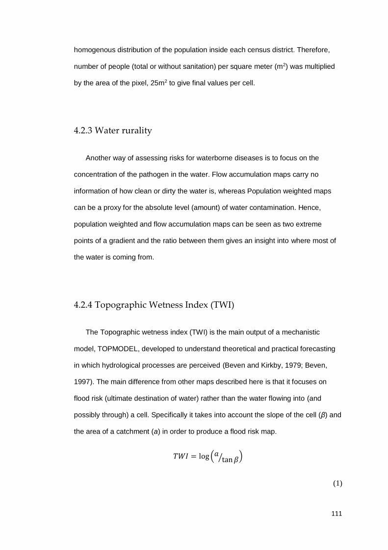
111

homogenous distribution of the population inside each census district. Therefore,

number of people (total or without sanitation) per square meter (m2) was multiplied

by the area of the pixel, 25m2 to give final values per cell.

4.2.3 Water rurality

Another way of assessing risks for waterborne diseases is to focus on the

concentration of the pathogen in the water. Flow accumulation maps carry no

information of how clean or dirty the water is, whereas Population weighted maps

can be a proxy for the absolute level (amount) of water contamination. Hence,

population weighted and flow accumulation maps can be seen as two extreme

points of a gradient and the ratio between them gives an insight into where most of

the water is coming from.

4.2.4 Topographic Wetness Index (TWI)

The Topographic wetness index (TWI) is the main output of a mechanistic

model, TOPMODEL, developed to understand theoretical and practical forecasting

in which hydrological processes are perceived (Beven and Kirkby, 1979; Beven,

1997). The main difference from other maps described here is that it focuses on

flood risk (ultimate destination of water) rather than the water flowing into (and

possibly through) a cell. Specifically it takes into account the slope of the cell (β) and

the area of a catchment (a) in order to produce a flood risk map.

𝑇𝑊𝐼 = log (𝑎tan 𝛽⁄ )

(1)

112

TWI states that areas with the same value would have the same hydrological

response to rainfall and hence are hydrologically similar. Higher values indicate that

an area/cell is more suitable for flooding and are caused by lower slopes (flat areas)

and/or convergence points of long slopes (Beven and Kirkby, 1979; Beven, 1997).

4.3 Model output

A dummy data set was created to exemplify how each map is produced. Then,

in the following section, the maps will be produced using real data from Salvador

city. Hence, given a digital elevation model (DEM) where each value is the elevation

information of a pixel,

DEM =

2 1 0

4 3 2

6 5 4

and a population map (P),

P =

0 4 3

0 0 0

6 0 0

Tarboton (1997) uses the elevation of the centre of the pixels to calculate

slope and flow direction. The method uses facets of a triangle to calculate the slope

of all eight neighbours cells and determine the steepest downward slope between

113

the eight planar triangular facets. Eight triangular facets are drawn from the centre of

the pixel to all its neighbours. Each of these facets will have a downslope vector

going outward from the centre and having an angle that falls within or outside of 45

degrees. The steepest vector is determined when the angle of the downslope vector

lie within the 45 degrees at the centre of the facet and this is assign the direction of

the flow. Once the steepest facet is identified, the proportion of flow to each slope

can be obtained based on equations 1-5 of Tarboton (1997) method. The flow

accumulation map (F) will produce a map showing the cumulative number of pixels

where the water is coming from assuming that all pixels received water, starting

from high to low elevated areas. The dark arrows indicate which pixels are receiving

the flow and where the flow is going to.

F =

1.6 4.2 9.0

1.4 2.0 2.6

1.0 1.0 1.0

Thus, for example, the value of 2.0 in the central cell is arrived at by adding

1.0 (the cell itself) to 0.6 from the bottom-left cell and 0.4 from the centre-left cell,

and so on. Note that the water can flow to more than one pixel given their elevation,

so a proportion of one pixel will flow to more than one downstream pixel if their

elevation is similar or equal. This is a feature of the model created by Tarboton

(1997). In this example, the pixel in the centre is receiving its water from itself and

the two pixels in the bottom line of the first two columns.

The flow accumulation threshold (T) can be applied by first defining a threshold

value (in this example we arbitrary define a value of 1.5) and everything that is

bigger than that value will be assigned a value of one, or otherwise zero. This map

114

displays a network of connected areas through which the water passes. The bigger

the threshold defined, the less complex is the network and the more it will represent

more permanent rivers/streams.

T =

1 1 1

0 1 1

0 0 0

Similar to the flow accumulation map, the population weighted map (PW) will

produce a map showing the cumulative number of people that the water would have

passed through. This map shows that even when there are no people living in the

pixel, the pixel still receives water from upslope populated areas. In this model, any

type of population information can be included. In the case of Salvador city, for

example (below), population density and people without sanitation were used to

produce two population weighted maps.

PW =

1.0 8.0 13

2.5 3.5 0

6.0 0 0

Now that Flow accumulation and the population weighted maps have been

generated, the water rurality map (W) can be produced based in the ratio between

them. The range of this measurement varies from zero to infinite, where zero means

that the water did not pass through any populated pixels before it reached the target

pixel, which happens with non-populated ridges areas, for example.

115

W =

0.6 1.9 1.4

1.7 1.8 0.0

6.0 0.0 0.0

The last map produced is the topographic wetness index (TWI), which from a

DEM, a slope can be generated, and TWI produced based on Equation 4.1. This

map indicates areas that are more likely to be flooded than others, higher values.

TWI =

7.7 8.7 13

6.8 7.1 7.5

6.5 6.5 6.6

Taking the second row and first column for demonstration, the flow

accumulation represents the catchment and is firstly transformed in area by

multiplying its values by the size of the pixel, five meters in this case (1.4 ∗ 5 = 7.05).

Then the TWI is the natural logarithm of the division between catchment area and

the tangent of the slope in radiants: log(7.050.0079⁄ ) = 6.8.

4.4 Application to Salvador city

A total of eight different sets of maps were generated as previously described,

using elevation data from Salvador, Brazil. To demonstrate the differences within

and between every map, at a range of scales, maps were generated in each case

for the whole of Salvador and also for a section of a neighbourhood of the city,

116

named Piraja. Figure 4.3 shows the digital elevation model itself for the whole city

and for Piraja, however, the other maps will be presented at three different scales,

going from local scale (Piraja), medium scale (Piraja and its region) to a city level

map.

Figure 4.3: Digital elevation model of Salvador, Brazil used to demonstrate the difference between risk maps. A community inside Salvador named Piraja (red area on top right map) was selected to illustrate the output of the model at a local scale.

The DEM of Salvador shows a city composed of many valleys in the whole area,

which makes the flow accumulation look heterogeneous, with higher and lower flow

accumulation areas, throughout the city (Figure 4.4). There is an extended area

with higher flow accumulation values going from middle to north in the flow

accumulation map for Piraja (Figure 4.4). In addition, the inclusion of streets into the

DEM makes the flow go to the streets in many cases, which can be seen to the

south of Piraja on Figure 4.4.

117

Figure 4.4: Flow accumulation risk map, which represents water flow. The map in the centre is the flow accumulation of a neighbourhood named Piraja. The bottom right is a medium scale map showing Piraja and its region and top right map is the flow accumulation for the whole city.

For the flow accumulation thresholds (Figures 4.5-4.7), the maps displayed a

connected network of runoff/rivers throughout the space. When the threshold is

higher, equal to 1000, fewer networks can be seen. For example, two more

extended paths are shown in the north and southwest of the map for Piraja in Figure

4.5. Then, if the threshold decreases to 500, more paths are connected to the main

path (Figure 4.6) and if the threshold decreases even more, to 50, there are more

short paths revealing a very complex network (Figure 4.7).

118

Figure 4.5: Flow accumulation threshold obtained from the Flow accumulation map, the threshold defined is 1000. The map in the centre is the flow accumulation threshold of a neighbourhood named Piraja. The bottom right is a medium scale map showing Piraja and its region and top right map is the flow accumulation threshold for the whole city.

119


120


The population weighted accumulation show a map with some patches of

homogenous low risk at the city level, which is associated with low density areas

(red and orange colours in Figure 4.8). However, looking at Piraja (local scale) in

Figure 4.8, it is possible to see that in those homogeneous areas, there are a few

lines associated with higher risk - for example a line path going from the centre to

the north of Piraja. This is an indication that the risk is coming from upslope dense

populated areas. Similarly, when the density of people without sanitation is

considered, the map shows a pattern associated with higher density areas of people

without sanitation, which in this case is concentrated at the north bound of the city

(top right map in Figure 4.9). In addition, at a local scale, the map show areas with

heterogeneous risk such as the southeast but also homogeneous areas, at the

north, with a line of higher risk locations (Figure 4.9).

121

Figure 4.8: Population weighted accumulation map showing the cumulative number of people where the water would have flown through. The map in the centre is the population weighted accumulation of a neighbourhood named Piraja. The bottom right is a medium scale map showing Piraja and its region and top right map is the population weighted accumulation for the whole city.

122

Figure 4.9: Population weighted accumulation map where is only considering the population density of people without sanitation. The map in the centre is the population weighted accumulation of a neighbourhood named Piraja. The bottom right is a medium scale map showing Piraja and its region and top right map is the population weighted accumulation for the whole city.

The water rurality map (Figure 4.10) represents how diluted the water is, where

the red colours represent a higher concentration of pathogens because most of the

water flowing to the pixel is coming from risky areas. The map in Figure 4.10 shows

an area at the centre of Piraja where the risk is very high and surrounded by low

risk. Finally, for the flooding risk map, measure by the TWI, the risk is very

heterogeneous and is evidently focused on streets in many cases, which it is

possible to see in the straight lines of higher values in the map (Figure 4.11).

123

Figure 4.10: Water rurality map obtained from the ratio between population weighted accumulation and flow accumulation. The map in the centre is the water rurality of a neighbourhood named Piraja. The bottom right is a medium scale map showing Piraja and its region and top right map is the water rurality for the whole city.

124

Figure 4.11: Topographic wetness index (TWI) map, which is a flooding risk map. The map in the centre is the TWI of a neighbourhood named Piraja. The bottom right is a medium scale map showing Piraja and its region and top right map is the TWI for the whole city.

4.5 Discussion

This chapter aimed to develop a range of topographical analyses that can be

used as measures of risk for waterborne diseases in public health. Even though the

direct association with waterborne diseases has not been addressed here, the

results should help to produce risk maps that can be used to understand

hydrological drivers of waterborne disease outcomes (see Chapter 3). The contrasts

between the results of each measurement demonstrate how complementary each

map can be in estimating the risk, and hence their importance.

The role of the environment in disease transmission has been increasingly

addressed recently and has been shown to be relevant in disease transmission.

Studies have either incorporated the environment in dynamic models of

125

transmission or have looked at how those variables are associated with diseases

outcomes. In dynamic modelling, hydrological transport of pathogens or rainfall-

runoff models have been integrated with epidemiological dynamic models (Bertuzzo

et al., 2007, 2008; Remais, Liang and Spear, 2008; Mari et al., 2012; Collender et

al., 2016; Rinaldo et al., 2017). For cholera, for example, the transport of pathogens

is assumed to happen through river networks and infection depends on the contact

rate between a susceptible individual and the river network (Bertuzzo et al., 2008;

Mari et al., 2012), whereas for schistosomiasis, the hydrological transport of the

pathogen occurs through the transport of the intermediate host (snail) which is

aquatic and gets carried out by runoff (Remais, Liang and Spear, 2008; Perez-Saez

et al., 2016). In addition, direct associations between flooding risk (TWI), river

density and leptospirosis have been found (Vega-Corredor & Opadeyi 2014). In

these different ways, the incorporation of the environment has helped explain

disease infection patterns. Here, our results can provide additional environmental

characteristics that have not been addressed yet but could improve our

understanding of the role of the environment in the dynamics of waterborne

diseases.

Flow accumulation thresholds provided a network map that can represent,

depending on the threshold defined, a network of temporary and/or permanent

rivers. Those maps carry information of where the possible runoff or river routes are,

which can be a risk for waterborne diseases due to the water mobilization of

pathogens. Complementary to flow accumulation threshold maps, flow accumulation

by itself carries information on how long the water travels before it reach a pixel,

which is indicative of the catchment area feeding the pixel. In that case, flow

accumulation can be hypothesized that the longer the water travels, more pathogen

is carrying, and hence, the risk of infection is higher.

126

On the other hand, while flow accumulation shows areas that receive more flow

than others, most of its flow can be coming from non/less populated area. That is

the difference between flow accumulation and population weighted maps. When

population data are incorporated, the data generated show the cumulative number

of people that the water might have passed through which can be a proxy for water

contamination or rat’s distribution in the case of leptospirosis. Despite using the

same principle (flow direction), maps produced by flow accumulation and population

weighted accumulation generated different patterns. Population weighted

accumulation showed high risk even in some non-populated areas because those

areas are receiving water from upslope-populated areas. In addition, the risk map

changed significantly when a map with sanitation information was produced, but,

there are higher risk areas in places with sanitation, indicating that the risk is mostly

coming from upslope areas that does not have sanitation.

The combination of hydrology and population data was inspired based on the

leptospirosis study in Salvador, Brazil. The issue came from the difficulty to obtain

high resolution data on rat’s distribution throughout the city. Alternatively, population

data can be seen as a proxy for the distribution of Norway rats as its occurrence can

be associated with human density (Boisier et al., 1997; Guan et al., 2009). However,

the use of population data go beyond that, Cryptosporidium, for example, is a

pathogen that are eliminated in the environment through human (and other

mammals) faeces, therefore, considering people without sanitation can be seen as a

risk for local and downstream contamination (Fayer, Speer and Dubey, 1997).

Furthermore, Katz et al (2006) observed that the reason of prolonged propagation of

Giardia during an outbreak in Boston was caused by person-to-person transmission,

indicating that population density can play a role in the transmission of giardiasis.

The topographic wetness index (TWI) has been used in epidemiology as noted

previously. The inclusion of this measurement in this chapter demonstrates how TWI

127

by itself does not catch all the hydrological variation in the environment such as the

water that flows through populated places. However, TWI combines flow

accumulation and slope of each cell in order to have a proxy of how likely it is for a

cell to be flooded. While flow accumulation may show large differences between

neighbouring cells, perhaps because some of them are receiving water from long

distance, the correction by the slope indicates if the water will be retained in a cell or

will just pass through. Therefore, even if a cell is receiving water from a short

distance (low flow), they might have the same likelihood of flooding as a cell that has

high flow, simply because of differences in slope.

A big contrast within water rurality map was observed, where the results showed

a patchier pattern with areas being either ‘dirty’ or ‘clean’. The reason for this

contrast is a combination of the population distribution throughout the city and the

water flow. The north area of the city is less populated, with most of the flow in those

areas coming from low or non-populated places, whereas in the other parts of the

city the opposite is the case. The population information used here were based on

district census, which varies with area and has been rescaled to the same scale of

the DEM. A better resolution of population density would result in a smoother

transition between ‘dirty’ and ‘clean’.

The maps produced here are considered proxies of water flow and do not

represent areas that will produce runoff or will be flooded every time it rains. To

predict runoff in the environment with high accuracy, it is necessary to collect a set

of many other factors such as high resolution rainfall data and soil permeability,

which makes the model very complex and expensive. Using topographic analysis

can be much cheaper and could be seen as an initial step in understanding not only

the dynamics of disease transmission in the environment but also the movement

and distribution of pathogens.

128

Therefore, the results shown her, demonstrate the usefulness of different

measurements of risk that can be applied to a range of waterborne diseases. These

features are important in terms of risk perception, which therefore changes

depending on the approach that has been used, or the approaches can be

complimentary. Use of these maps may help organizations and governments to

understand patterns of infection and derive actions to reduce transmission.

4.6 References

Atwill, E.R., Hou, L., Karle, B.M., Harter, T., Tate, K.W. & Dahlgren, R.A. (2002).

Transport of Cryptosporidium parvum oocysts through vegetated buffer strips

and estimated filtration efficiency. Applied and environmental microbiology, 68,

5517–27.

Auld, H., MacIver, D. & Klaassen, J. (2004). Heavy rainfall and waterborne disease

outbreaks: the Walkerton example. Journal of Toxicology and Environmental

Health, Part A, 67, 1879–1887.

Berry, D.F. & Hagedorn, C. (1991). Soil and groundwater transport of

microorganisms. Biotechnology (Reading, Mass.), 15, 57–73.

Bertuzzo, E., Azaele, S., Maritan, A., Gatto, M., Rodriguez-Iturbe, I. & Rinaldo, A.

(2008). On the space-time evolution of a cholera epidemic. Water Resources

Research, 44.

Bertuzzo, E., Maritan, A., Gatto, M., Rodriguez-Iturbe, I. & Rinaldo, A. (2007). River

networks and ecological corridors: Reactive transport on fractals, migration

fronts, hydrochory. Water Resources Research, 43.

Beven, K.J. (1997). Distributed hydrological modelling : applications of the

129

TOPMODEL concept. John Wiley & Sons.

Beven, K.J. & Kirkby, M.J. (1979). A physically based, variable contributing area

model of basin hydrology / Un modèle à base physique de zone d’appel

variable de l’hydrologie du bassin versant. Hydrological Sciences Bulletin, 24,

43–69.

Boisier, P., Rasolomaharo, M., Ranaivoson, G., Rasoamanana, B., Rakoto, L.,

Andrianirina, Z., Andriamahefazafy, B. & Chanteau, S. (1997). Urban epidemic

of bubonic plague in Majunga, Madagascar: epidemiological aspects. Tropical

Medicine & International Health, 2, 422–427.

Cann, K.F., Thomas, D.R., Salmon, R.L., Wyn-Jones, A.P. & Kay, D. (2013).

Extreme water-related weather events and waterborne disease. Epidemiology

and infection, 141, 671–86.

Collender, P.A., Cooke, O.C., Bryant, L.D., Kjeldsen, T.R. & Remais, J. V. (2016).

Estimating the microbiological risks associated with inland flood events:

Bridging theory and models of pathogen transport. Critical reviews in

environmental science and technology, 46, 1787–1833.

Collier, S.A., Stockman, L.J., Hicks, L.A., Garrison, L.E., Zhou, F.J. & Beach, M.J.

(2012). Direct healthcare costs of selected diseases primarily or partially

transmitted by water. Epidemiology and Infection, 140, 2003–2013.

Costa, F., Porter, F.H., Rodrigues, G., Farias, H., de Faria, M.T., Wunder, E.A.,

Osikowicz, L.M., Kosoy, M.Y., Reis, M.G., Ko, A.I. & Childs, J.E. (2014).

Infections by Leptospira interrogans, Seoul virus, and Bartonella spp. among

Norway rats (Rattus norvegicus) from the urban slum environment in Brazil.

Vector borne and zoonotic diseases (Larchmont, N.Y.), 14, 33–40.

Crowther, J., Wyer, M.D., Bradford, M., Kay, D. & Francis, C.A. (2003). Modelling

130

faecal indicator concentrations in large rural catchments using land use and

topographic data. Journal of Applied Microbiology.

Curriero, F.C., Patz, J.A., Rose, J.B. & Lele, S. (2001). The association between

extreme precipitation and waterborne disease outbreaks in the United States,

1948-1994. American journal of public health, 91, 1194–9.

Davies, C.M., Ferguson, C.M., Kaucner, C., Krogh, M., Altavilla, N., Deere, D.A. &

Ashbolt, N.J. (2004). Dispersion and transport of Cryptosporidium Oocysts from

fecal pats under simulated rainfall events. Applied and environmental

microbiology, 70, 1151–9.

Edwards, D.R., Coyne, M.S., Vendrell, P.F., Daniel, T.C., Moore, P.A. & Murdoch,

J.F. (1997). Fecal coliform and streptococcus concentrations in runoff from

grazed pstures in northwest Arkansas. Journal of the American Water

Resources Association, 33, 413–422.

Fayer, R., Speer, C.A. & Dubey, J.P. (1997). The general biology of

Cryptosporidium. Cryptosporidium and Cryptosporidiosis, pp. 1–42. CRC Press

Inc.

Ferguson, C.M., Croke, B.F.W., Beatson, P.J., Ashbolt, N.J. & Deere, D.A. (2007).

Development of a process-based model to predict pathogen budgets for the

Sydney drinking water catchment. Journal of water and health, 5, 187–208.

Garba, B., Bahaman, A.R., Khairani-Bejo, S., Zakaria, Z. & Mutalib, A.R. (2017).

Retrospective Study of Leptospirosis in Malaysia. EcoHealth, 1–10.

Gaynor, K., Katz, A.R., Park, S.Y., Nakata, M., Clark, T.A. & Effler, P. V. (2007).


campus. The American journal of tropical medicine and hygiene, 76, 882–5.

Guan, P., Huang, D., He, M., Shen, T., Guo, J. & Zhou, B. (2009). Investigating the

131

effects of climatic variables and reservoir on the incidence of hemorrhagic fever

with renal syndrome in Huludao City, China: a 17-year data analysis based on

structure equation model. BMC infectious diseases, 9, 109.

Herrera, D., Ellis, A., Fisher, B., Golden, C.D., Johnson, K., Mulligan, M., Pfaff, A.,

Treuer, T. & Ricketts, T.H. (2017). Upstream watershed condition predicts rural

children’s health across 35 developing countries. Nature Communications, 8,

811.

Jamieson, R., Gordon, R., Joy, D. & Lee, H. (2004). Assessing microbial pollution of

rural surface waters: A review of current watershed scale modeling

approaches. Agricultural Water Management, 70, 1–17.

Jenson, S.K. & Domingue, J.O. (1988). Extracting topographic structure from digital

elevation data for geographic information-system analysis. Photogrammetric

Engineering and Remote Sensing, 54, 1593–1600.

Katz, D.E., Heisey-Grove, D., Beach, M., Dicker, R.C. & Matyas, B.T. (2006).

Prolonged outbreak of giardiasis with two modes of transmission. Epidemiology

and infection, 134, 935–41.

Ko, A.I., Reis, M.G., Dourado, C.M.R., Johnson, W.D. & Riley, L.W. (1999). Urban

epidemic of severe leptospirosis in Brazil. The Lancet, 354, 820–825.

Lau, C.L., Smythe, L.D., Craig, S.B. & Weinstein, P. (2010). Climate change,


Royal Society of Tropical Medicine and Hygiene, 104, 631–638.

Mahajan, R., Uber, J.G. & Eisenberg, J.N.S. (2014). A Dynamic Model to Quantify

Pathogen Loadings from Combined Sewer Overflows Suitable for River Basin

Scale Exposure Assessments. Water Quality, Exposure and Health, 5, 163–

172.

132

Mari, L., Bertuzzo, E., Righetto, L., Casagrandi, R., Gatto, M., Rodriguez-Iturbe, I. &


mobility and sanitation. Journal of the Royal Society, Interface, 9, 376–88.

Medema, G.. & Schijven, J.. (2001). Modelling the sewage discharge and dispersion

of cryptosporidium and giardia in surface water. Water Research, 35, 4307–

4316.

O’Callaghan, J.F. & Mark, D.M. (1984). The extraction of drainage networks from

digital elevation data. Computer Vision, Graphics, and Image Processing, 28,

323–344.

Ozioma Forstinus, N., Emmanuel Ikechukwu, N., Paul Emenike, M., Ogonna

Christiana, A. & Kumar Nalla, A. (2016). Water and Waterborne Diseases: A

Review. International Journal of TROPICAL DISEASE & Health India. Nwabor

et al, 12, 1–14.

Pappachan, M.J., Sheela, M. & Aravindan, K.P. (2004). Relation of rainfall pattern

and epidemic leptospirosis in the Indian state of Kerala. Journal of

epidemiology and community health, 58, 1054.

Perez-Saez, J., Mande, T., Ceperley, N., Bertuzzo, E., Mari, L., Gatto, M. & Rinaldo,

A. (2016). Hydrology and density feedbacks control the ecology of intermediate

hosts of schistosomiasis across habitats in seasonal climates. Proceedings of

the National Academy of Sciences of the United States of America, 113, 6427–

32.

Prüss, A., Kay, D., Fewtrell, L. & Bartram, J. (2002). Estimating the Burden of

Disease from Water, Sanitation, and Hygiene at a Global Level. Environmental

Health Perspectives, 110.

Remais, J., Liang, S. & Spear, R.C. (2008). Coupling Hydrologic and Infectious

133

Disease Models To Explain Regional Differences in Schistosomiasis

Transmission in Southwestern China. Environmental Science & Technology,

42, 2643–2649.

Rinaldo, A., Bertuzzo, E., Blokesch, M., Mari, L. & Gatto, M. (2017). Modeling Key

Drivers of Cholera Transmission Dynamics Provides New Perspectives for

Parasitology. Trends in Parasitology, 33, 587–599.

S. E. Walker, S.E., S. Mostaghimi, S., T. A. Dillaha, T.A. & R E. Woeste, R.E.

(1990). Modeling animal waste manegment practices: impacts on bacteria

levels in runoff from agricultural lands. Transactions of the ASAE, 33, 0807–

0817.

SUMI, A., TELAN, E.F.O., CHAGAN-YASUTAN, H., PIOLO, M.B., HATTORI, T. &

KOBAYASHI, N. (2017). Effect of temperature, relative humidity and rainfall on

dengue fever and leptospirosis infections in Manila, the Philippines.

Epidemiology and Infection, 145, 78–86.

Tarboton, D.G. (1997). A new method for the determination of flow directions and

upslope areas in grid digital elevation models. Water Resources Research, 33,

309–319.

Tian, Y.Q., Gong, P., Radke, J.D. & Scarborough, J. (2002). Spatial and Temporal

Modeling of Microbial Contaminants on Grazing Farmlands. Journal of

Environment Quality, 31, 860.

Vega-Corredor, M. & Opadeyi, J. (2014). Hydrology and public health: linking human

leptospirosis and local hydrological dynamics in Trinidad, West Indies. Earth

Perspectives, 1, 3.

WHO. (2003). Emerging issues in water and infectious disease. World Health

Organization, Geneva.

134

WHO. (2015). Progress on sanitation and drinking water – 2015 update and MDG

assessment. World Health Organization.

Yang, K., LeJeune, J., Alsdorf, D., Lu, B., Shum, C.K. & Liang, S. (2012). Global

distribution of outbreaks of water-associated infectious diseases. PLoS

neglected tropical diseases, 6, e1483.

135

Chapter 5: 14 years of leptospirosis

surveillance in Salvador city, Brazil: spatial

distribution of leptospirosis cases and its

relationship with hydrology

5.1 Introduction

From 1990, the world urban population had approximately doubled its size by

2015, going from 2.3 billion to 4 billion people living in urban areas. Most of this

change came from low income countries in Asia, Africa and Latin America. Despite

many efforts to reduce the number of urban slum settlements, in developing

countries 880 million people lived in urban slums (low income settings) in 2015,

which represents a substantial increase in comparison with 690 million in 1990

(Moreno et al., 2016). This drastic change in human demographics changed the

epidemiology of human leptospirosis, a disease caused by spirochete bacteria

(Leptospira spp.). The transmission of the disease involves complex interactions

between the animal reservoir, human demographics and the environment, where the

infection can occur through direct or indirect contact with urine of an infected animal

or water contaminated with urine.

Historically, human leptospirosis mostly occurred in rural settings such as rice

plantations, mining and livestock farms (Faine, 1982; Waitkins, 1986; Katz, Manea

and Sasaki, 1991; Faine et al., 1999). However, nowadays, human leptospirosis is

considered an occupational disease in tropical countries occurring, mainly, in low

income including urban settings (Albert I Ko et al., 1999; Felzemburgh et al., 2014a;

Costa, Hagan, et al., 2015; Torgerson et al., 2015). The risk factors associated with

the infections are related to socioeconomics and environmental characteristics such

136

as lower levels of income and distance to an open sewer (Albert I Ko et al., 1999;

Barcellos and Sabroza, 2001a; Sarkar et al., 2002; Maciel et al., 2008; Reis et al.,

2008; Ko, Goarant and Picardeau, 2009; Oliveira et al., 2009). In addition, outbreaks

of the disease have been observed after heavy rainfall and flooding, and also, peaks

in the number of cases have been observed during rainy seasons in endemic areas

(Albert I Ko et al., 1999; Barcellos and Sabroza, 2001b; Smythe et al., 2002; Jena,

Mohanty and Devadasan, 2004; Gaynor et al., 2007; Desvars et al., 2011b; Blanco

and Romero, 2015; Gutiérrez and Martínez-Vega, 2018). For example, Ko et al

(1999) observed an association between an outbreak that occurred in Salvador,

Brazil two weeks after heavy rainfall and flooding in 1996. Similarly, many other

studies reported leptospirosis outbreaks after heavy rainfall and flooding such as

Malaysia in 2000 and 2010, Guyana 2005, New Caledonia in 2008, Philippines in

2009, Fiji in 2012 and many others (see Lau et al (2010b)).

These findings, which did not in themselves aim to look the spatial distribution of

the cases, led to explorations of the spatial variation of human leptospirosis (i.e. at

the community level) and its association with environmental variables. Schneider et

al. (2012), for example, identified that municipalities closer to the Pacific ocean in

Nicaragua have more cases of leptospirosis. Average precipitation over the previous

two months, maximum precipitation and the rural proportion of the population were

the main drivers that explained the spatial distribution of cases. In American Samoa,

the distribution of cases was associated with factors at the environmental

household-level as well as individual factor-levels, and four spatial clusters were

identified (Lau et al., 2012). Occupation, knowledge of leptospirosis and gender

were individual factors associated with cases, whereas the environmental factors

were vegetation and soil type. In China, the use of spatial techniques combined with

time (spatiotemporal analysis) not only helped to observe a decline in the number of

137

cases from 2005-2015 at county level but also observed a decreased disease

burden in endemic areas (Dhewantara et al., 2018).

Vega-Corredor & Opadeyi (2014), in a study of human leptospirosis cases

between communities in Trinidad, used a Geographic Information System (GIS)

approach in order to generate water-related environmental variables such as rainfall,

proportion of soil free drainage, proportion of imperfect/impeded drainage soil, river

density and the topographic wetness index (TWI). Firstly, their study observed

evidence of spatial variation in cases between communities. Secondly, rainfall,

imperfect/impeded drainage soil and TWI were associated with those cases, where

rainfall and imperfect/impeded drainage soil had a stronger association with cases in

the south, and TWI had higher odds ratios in the north of the island. Their spatial

scale looked at cases at a county level, which gave them a large areal coverage but

low resolution.

The addition of spatial data at a regional level in human leptospirosis studies in

Trinidad confirms that the environment has an important role to play in the spatial

variation of cases. This was only possible due to the use of spatial statistics and GIS

techniques, which allowed associations with disease outcomes to be explored, given

the evaluation of spatial dependency. Although rainfall has been demonstrated to be

associated with leptospirosis cases world-wide, with the exception of the study of

Vega-Corredor & Opadeyi (2014), the exploration of other hydrological variables has

not been addressed previously. Human leptospirosis can be considered a

waterborne disease, and so other water-related variables can be associated with

disease outcomes, as shown by Vega-Corredor & Opadeyi (2014). Chapter Four

developed a set of different hydrological variables based on topographical and

population data, which have been shown to be complementary to each other. These

hydrological variables are designed to track the path of the rainfall once it has

reached the ground. Looking for an association with those variables can be very

138

informative about the mechanisms of transmission of the disease. Therefore, this

chapter will evaluate the spatial distribution of human leptospirosis cases in

Salvador, Brazil and make inferences about how those cases might be associated

with the hydrology of the city.

5.2 Material and methods

5.2.1 Study area

The study was carried out in Salvador, a city located in the northeast of Brazil,

which is the third biggest city in the country. Salvador is divided into approximately

4000 census districts used by the Brazilian Institute of Geography and Statistics

(IBGE) to perform census counts and collect other demographic information on the

population. The latest census performed in Brazil is from 2010 and will be used here

to generate population counts for each district.

Human leptospirosis is endemic in Salvador with seasonal peaks every rainy

season. In 1996, the city had an outbreak reported later by Ko et al (1999) who

evaluated the epidemiology of the outbreak and helped to implement protocols for

surveillance of the disease. Until 2010, all the suspected cases of human

leptospirosis were designated to Couto Maia hospital, an infectious disease state

hospital, for treatment and confirmatory diagnosis. After 2010, the protocol for the

diagnosis of leptospirosis changed, which changed the coverage of the surveillance,

whereby more hospitals could receive suspected cases and perform laboratorial

diagnoses.

5.2.2 Data collection and case definition

139

Since the outbreak in 1996, the Oswaldo Cruz Foundation (Fiocruz) has been

conducting active population-based surveillance in Salvador. This is a collaboration

together with the state and city’s secretaries of health. The surveillance is conducted

in the reference hospital for infectious disease diagnosis and treatment, Couto Maia

Hospital, where a prospective analysis is performed on each patient admitted into

the hospital. The clinical definition of severe human leptospirosis is: acute

undifferentiated fever associated with either bleeding, acute renal failure, jaundice,

or acute liver injury with transaminases <1,000 U/L (Nabity et al., 2012).

Each individual who fulfilled the criteria for a clinical suspicion of severe

leptospirosis was asked for their consent to participate in the study. Once consent

was given, the patients were submitted to a questionnaire to collect demographic

information, symptoms, length of hospital stay and outcome (discharged). The

protocol was approved by the hospital, the Oswaldo Cruz Foundation, the Brazilian

National Commission for Ethics in Research and Yale University. All individuals

admitted with clinical leptospirosis between 1996 and 2010 were included in the

study. The data were grouped by census district and this will be the scale of the

analysis carried out here.

5.2.3 Hydrological data

The hydrological data used in this chapter were produced based on a

topographical (elevation) map layer obtained from CONDER, the urban planning

department of Salvador. This map had squared pixels of 5 meters resolution

containing the elevation information and was used to produce a set of four different

hydrological maps. The main assumption is that once water has reached the

ground, it will become runoff and will flow to the lowest point in the surface. Flow

accumulation, population weighted accumulation (PWA), water rurality and

140

topographic wetness index (TWI) are the maps used here (see Chapter 4). Flow

accumulation represents how far the water have travelled through the surface until

reaches a pixel, in other words, it is the cumulative number of pixels that the water

has flown through. Similarly, PWA represents the number of people the water would

have passed through which can be used as a proxy for water contamination. PWA

was generated with a combination of demographic data obtained from 2010

population census and was re-scaled to the same resolution as the topographical

map. Water rurality is the ratio between flow accumulation and PWA and can

represent a spectrum of water contamination (more rural or urbanised areas). The

TWI has been used previously by Vega-Corredor & Opadeyi (2014) and evaluates

the likelihood of a pixel being flooded given its flow accumulation and the slope. The

higher the value the more likely is a pixel to be flooded. All the maps were produced

using MATLAB. For an in depth description of the methods please see the previous

chapter.

There is a difference in the resolution between hydrological maps and the

recorded number of leptospirosis cases. The former were obtained with very high

resolution (hydrological information every five meters), whereas the latter was the

observation of cases at district level. The hydrological data were grouped inside the

areas of each district and the 90th quantile of the range of values was obtained. The

decision to use quantiles rather than averages was made with the intention of

reflecting the spectrum of the hydrological values that represent a risk for

leptospirosis. The histogram of the values in each district is very right skewed, with

large numbers of small values. Hence, averages would not capture the true

distribution of values at district level.

5.3 Statistical analysis

141

Statistical analysis was performed in three steps: development of a non-spatial

model, seeking evidence of spatial variation in the data, and development of a

geostatistical model. The non-spatial model was developed to select covariates to

further evaluate if there was spatial variation in the predictions. Once the evidence

of spatial variation was shown, the geostatistical model was developed.

5.3.1 Non-spatial model

Let 𝑌𝑖 denote the total number of human leptospirosis cases and 𝑃𝑖 the

population of each ith census district of Salvador. The generalised linear mixed

effects model assumes that 𝑌𝑖 are conditionally independent observations of the

random effect 𝑍𝑖. Hence, 𝑌𝑖 are Poisson distributed with expectation 𝑒𝜂𝑖

𝑌𝑖|𝑍𝑖 ~ 𝑃𝑜𝑖𝑠𝑠𝑜𝑛 ( 𝑒𝜂𝑖 )

where,

𝜂𝑖 = log 𝑃𝑖 + 𝑋𝛽 + 𝑍𝑖 + 𝑒𝑖

𝑃𝑖 is the offset for the population; 𝛽 is a vector of the coefficients for the

explanatory variables; 𝑋 is the design matrix containing the variables for the fixed

effects; 𝑍𝑖 is a vector of unobservable random effects which follows a multivariate

normal distribution centered at zero with variance 𝐷, where 𝐷 is diagonal with entry

of the unknown vector of random effects; 𝑒𝑖 is the residual variance assumed to be

normally distributed 𝑒𝑖 ~ 𝑁(0, 𝜎2). The analysis was performed using R software,

function glmer() from the package lme4.

There are four explanatory (hydrological) variables which were selected via

nested model selection - flow accumulation, PWA, water rurality and TWI. The

mixed effects model used the district census as a random effect and the

142

hydrological variables as fixed effects. The first step of the model selection is to

compare univariate models against a null model. This comparison was ranked from

the most significantly different to the least from the null model. The models which

were not significantly different from the null model were removed from the next steps

because this indicates that they are not associated with human leptospirosis cases.

The model with the highest rank was considered a baseline and the remaining

variables were added individually as candidate new models. The same process was

then used in comparing the baseline model with the new candidate models. If the

candidate model was significant different from the baseline, then it was ranked and

the same process repeated until no more variables could be added into the model.

5.3.2 Empirical variogram

Empirical variograms are used to describe the degree of spatial dependency in a

set of data, hence demonstrating whether closer locations are more similar than far

locations. A semivariogram of each paired location was calculated and its distance

recorded. If there is evidence of spatial dependency, the semivariogram values

would be smaller for points closer to each other, and the values should increase

until reaching, in most of the cases, an asymptote.

There are three components of the empirical variogram: the nugget, sill and

range. The nugget represents the variation which is not explained by spatial

location, in other words, it is the semivariogram evaluated right after a zero meter

distance. The sill is where the semivariogram values reaches an asymptote. Finally,

the range is where the semivariogram values reaches 95% of the sill. Practically, the

nugget will give an insight as to whether there is unexplained variance that space

does not capture, and the range is the distance interval over which all the

observations are spatially dependent.

143

Another feature to be considered when exploring spatial dependency with

empirical semivariograms is the direction of the dependency. Some diseases can

spread more in one direction than another and this represents an uneven spread

(for example, airborne diseases downwind of a source). Here, for leptospirosis

studies, it is assumed to be evenly spread in all directions, which is called an

isotropic process. In this case, the semivariogram obtained from a point a to b is the

same as the semivariogram from point b to a. The last feature is that there is no

temporal dependency from the data observed, which are assumed to be stationary.

Therefore, the variogram for each unit distance 𝑢 is:

𝑣(𝑢) = 𝜏2 + 𝜎2 ∗ (1 − 𝑝(𝑢))

where, 𝑢 is a vector of the Euclidean distances between locations 𝑥 and 𝑥′ that

was used to evaluate the variogram; 𝜏2 is the nugget effect; 𝜎2 is the variance of the

spatial process and 𝑝(𝑢) is the spatial correlation function. An exponential

correlation function was used as 𝑝(𝑢) and is a special case of the Matern correlation

function where the smoothness parameter is fixed at 𝜅 = 0.5 (see Giorgi & Diggle

(2017) for the Matern correlation function). The validity of the correlation function

was explored through Monte Carlo simulations which evaluate if the empirical

variogram is different from what would be expected if there was no spatial

dependency.

The analysis was performed using R software. The predicted random effects of

the non-spatial model were extracted using the function ranef() from the package

lme4 and the empirical variogram was generated using the package PrevMap and

function spat.corr.diagnostic().

5.3.3 Geostatistical model

144

A geostatistical model assumes that 𝑌𝑖 are realisations of a continuous space

such that 𝑌𝑖 are dependent observations of an unobserved spatial stochastic

process 𝑆(𝑥𝑖). Therefore, the total number of cases 𝑌𝑖 given the location 𝑥𝑖: 𝑖 =

1, … , 𝑛 is Poisson distributed:

𝑌𝑖|𝑆(𝑥𝑖) ~ 𝑃𝑜𝑖𝑠𝑠𝑜𝑛(𝑒𝜂(𝑥𝑖)) 𝑓𝑜𝑟 𝑖 = 1, … , 𝑛

where,

𝜂(𝑥𝑖) = log 𝑃𝑖 + 𝑑(𝑥𝑖)′𝛽 + 𝑆(𝑥𝑖) + 𝑍𝑖

𝑃𝑖 is the population of each district; 𝑑(𝑥𝑖) is a vector of explanatory variables

associated with location i; 𝛽 is a vector with the coefficients for each explanatory

variables; 𝑆(𝑥𝑖) is the structured random effect that accounts for the spatial

dependency which is an isotropic and stationary Gaussian process with mean zero,

variance 𝜎2 and correlation function 𝜌(𝑥, 𝑥′) = 𝐶𝑜𝑟𝑟[𝑆(𝑥), 𝑆(𝑥′)] where 𝑥 and 𝑥′ are

two distinct locations. 𝑍𝑖 are the unstructured random effects that account for the

variance that is not explained by the space and is normally distributed with mean

zero and variance 𝜏2.

The spatial process is assumed to be stationary and isotropic, hence

𝐶𝑜𝑟𝑟[𝑆(𝑥), 𝑆(𝑥′)] = 𝜌(‖𝑥 − 𝑥′‖), where ‖ . ‖ indicates Euclidean distance. A Matern

correlation function 𝜌(𝑢; 𝜙, 𝜅) was used with a smoothness parameter fixed at 𝜅 =

0.5 and 𝜙 being the scale of the spatial correlation. See Giorgi & Diggle (2017) for a

description of the Matern correlation function and the method of estimating the

spatial model. The routine is an example of Monte Carlo Maximum Likelihood

(MCML) which uses an importance sampling in order to approximate the likelihood

function and estimate the parameters from the model. All the statistical analysis

145

were performed using the R software, function poisson.log.MCML() from the

package PrevMap.

5.3.4 Model validation

The correlation function was validated using a variogram algorithm to simulate

data and compare with the results observed. This process was obtained from that

described in Macharia et al. (2018) which was developed in the PrevMap package.

The process consists of simulating data under the fitted model, computing a

variogram and obtaining a 95% envelop of the empirical variogram. If the estimated

variogram falls within the 95% envelope, indicates that there is no further spatial

variation and the adopted spatial correlation function was considered sufficient.

5.3.5 Identification of areas with high risk of leptospirosis

transmission

From the geostatistical model, a target 𝑇 can be defined for predictive inference.

Here, the interest is to identify areas that have more cases of leptospirosis than

expected. It is assumed that those areas would have a higher risk of leptospirosis

transmission. The baseline incidence of leptospirosis in Salvador will be estimated

by 𝛼, which is the intercept of the linear predictor. The predicted incidence of

leptospirosis for each location and its confidence interval can be given by

�̂� (�̂�0.25; �̂�97.5). Areas with high risk of leptospirosis would be the ones where the

lower confidence interval is greater than the baseline incidence. This indicates that

those areas have an incidence rate higher than expected.

𝑇𝑖 = {𝑥: (�̂�0.25(𝑥𝑖) − 𝛼) > 0} 𝑖 = 1, … , 𝑛;

146

5.3.6 Risk of having at least one case of human leptospirosis

From the predicted incidence of leptospirosis obtained in the geostatistical

model, another great interest for public health management can be extracted,

namely, finding the risk of a census district having at least on case of leptospirosis.

This can be defined as the probability of 𝑌𝑖 being bigger than zero, hence, the target

can be defined as:

𝑇𝑖 = 𝑃(𝑌𝑖 > 0|𝑆(𝑥𝑖)) = 1 − 𝑒−𝑒 �̂�(𝑥𝑖) 𝑖 = 1, … , 𝑛;

5.4 Results

In total, 2168 individuals were admitted to Couto Maia Hospital with clinical

leptospirosis between 1996 and 2010. However, there were some cases where

explanatory variables were absent. The total number of cases used in the

regression analysis was 2010 and the total number of districts was 3412. The

average number of cases per district was 0.59±1.15 (SD) where the maximum

number of cases reported was 13. Approximately, 31% (N=1060) of the districts had

cases reported. Figure 5.1 shows the distribution of cases in each district of

Salvador, Brazil, where most of the districts with the highest numbers of cases are

located in the northwest of the city. Figure 5.2 shows the distribution of the

aggregated values of the covariates in each district census of Salvador city. Flow

accumulation and TWI had higher values in the north of the city whereas PWA and

water rurality had lower values.

147

Figure 5.1: Distribution of human leptospirosis cases in the city Salvador, Brazil. The cases were obtained from active surveillance in Couto Maia Hospital from 1996-2010.

Figure 5.2: Hydrological explanatory variables of Salvador, Brazil used in the analysis. The values were aggregated from each census district where the 90th quantile was obtained.

148

The model selection results indicate that only water rurality was associated with

leptospirosis cases in Salvador, Brazil (Table 5.1). The other covariates were not

significantly different from the null model and were not used in the rest of the

analysis. The empirical variogram of the predicted random effects demonstrated that

there was spatial dependency in the predictions of the mixed effects model, which

supports the use of spatial analysis (Figure 5.3).

Table 5.1: Results of the model selection base on likelihood ratio test where all the models were compared against the null model. (k is the difference on the number of parameters; LogLik is the log likelihood of the model)

LogLik k p-value

Null model -3482.62 - -

Population weighted accumulation -3482.46 1 0.58

Flow accumulation -3482.22 1 0.37

Topographic wetness index -3482.27 1 0.40

Water rurality -3474.75 1 0.00007

Figure 5.3: Empirical variogram of the predicted random effects from the best model selected. The grey area in the graph indicates the interval where the variogram is not different from what is expected by chance.

149

The correlation function of the spatial model was validated by simulation and

Figure 5.4 show the envelope (grey shade) and the empirical variogram estimated

(dark lines). The empirical variogram lay inside the envelope and indicates that there

is no spatial dependency in the model and the correlation function used was

appropriate. The practical range for an exponential function is three times the scale

of the spatial dependency estimated which is approximately 12km. The model

estimated two types of variance that are not explained by the linear predictor, the

spatial structured variance (𝜎2) and the unstructured variance (𝜏2) (Table 5.2).

Table 5.2: Estimated coefficients of the geostatistical model. The first two rows are the predictors presented as odd ratio whereas 𝜎2 is the variance of the Gaussian process, 𝜙 is the scale of the spatial

correlation and 𝜏2 is the variance of the nugget effect. (CI= Confidence interval)

Estimates Lower CI Upper CI

Intercept 0.0002 0.0001 0.0006

Water rurality 0.7973 0.6964 0.9128

𝜎2 1.0456 0.4122 2.6528

𝜙 4.2599 1.4617 12.4148

𝜏2 1.0167 0.1592 6.4924

150

Figure 5.4: Validation of the empirical variogram estimated in the spatial model. Grey shade represent the 95% interval of the variogram and dark line is the variogram estimated.

Water rurality was the only covariate selected in the model selection process

and the results of the regression shown that water rurality is negatively associated

with human leptospirosis cases (Table 5.2). The predicted incidence per 10,000

people and 95% confidence interval are shown in Figure 5.5, Figure 5.6 and Figure

5.7. The northwest and centre of Salvador city are the regions where the predicted

incidence per 10,000 people (Figure 5.5) and the risk of having at least one case of

leptospirosis (Figure 5.8) are higher. However, areas where there were more cases

than expected extended from the northwest, passing through the west and a few

places in the south of the city (Figure 5.9). The standardized residual plot can be

seen in Figure 5.10.

2 4 6 8 10 12

0.4

0.6

0.8

1.0

1.2

1.4

Distance (Km)

Em

pir

ica

l va

rio

gra

m

151

Figure 5.5: Predicted leptospirosis incidence per 10,000 population in Salvador, Brazil obtained from the geostatistical model.

Figure 5.6: Lower confidence interval of the predicted leptospirosis incidence per 10,000 population of Salvador, Brazil.

152

Figure 5.7: Upper confidence interval of the predicted leptospirosis incidence per 10,000 population in Salvador, Brazil.

Figure 5.8: Risk of having one case or more of human leptospirosis in each census district of Salvador, Brazil.

153

Figure 5.9: Areas with incidence of human leptospirosis in Salvador Brazil. Higher and lower than expected are shown in the colours orange and green, respectively.

Figure 5.10: Standardized residual plot.

154

5.5 Discussion

This chapter aimed to explore the association between human leptospirosis

and hydrological variables by looking at the total number of cases per district census

and extreme (ninetieth percentile) hydrological values. A set of new hydrological

variables was developed that are complementary to each other and can be used as

measures of environmental risk for waterborne diseases such as leptospirosis.

Before going into the results it is perhaps useful to reiterate the meaning of each

hydrological variable and the motivation behind the use of extreme values in the

statistical analysis. These explanations will help to understand how each

hydrological variable can be translated into risk and how these risks can be

associated with leptospirosis infections. There were four hydrological variables

extracted from a Digital Elevation Model - flow accumulation, population weighted

accumulation (PWA), water rurality and the topographic wetness index (TWI).

Flow accumulation can be considered as the area of a catchment because it

summarises all the upslope cells that water flows through until it reaches a target

cell. For that reason, it is possible to say that flow accumulation gives information on

how far the runoff water has flown over the surface, but also how much water has

been ‘collected’ since the same amount of water originally fell on each cell. In the

context of waterborne diseases, it can be considered as a way of describing the

abundance of pathogen reaching a cell by assuming simply that more water implies

more pathogen. Similarly, PWA can be thought of as either an area or an amount,

but in this case weighted by how populated areas are. Hence, the assumption might

be that water that flows through populated areas carries more pathogens because

more populated areas have more human waste and garbage and more rats.

Alternatively, we might propose that water that flows through populated areas

155

carries fewer pathogens because in more populated areas water tends to flow over

paved surfaces and has less opportunity to acquire pathogens. Furthermore, if a

ratio between those two measurements is taken, it is possible to scale the origin of

the water arriving in a targeted cell, independent of quantity. This ratio is given by

‘water rurality’ and higher values indicate the water is coming from more populated

areas whereas lower values indicate water is coming from non-populated areas.

Finally, TWI is a commonly used as a proxy for flood risk as it takes to account the

catchment area (flow accumulation) and the slope. Higher values are indicative of a

higher likelihood of flooding. In the present context, therefore, it is assumed that the

higher is the likelihood of flooding, the larger the number of pathogens that will

accumulate in a target cell (rather than simply passing through).

The hydrological variables were calculated at a very fine scale, five meters

resolution. On the other hand, human leptospirosis cases were taken at a district

level. To match the scale of the observed disease cases, the hydrological data had

to be aggregated at the district level. The first exploration on the data showed that

the distribution of the hydrological values for all variables were very right skewed,

showing a lot of small values and a very few higher values. These results were

expected at that scale due to the topography of the city. The city is not flat but is

composed of many valleys (Figure 5.11). This characteristic means that each district

has a very high variation of values and few very large values in the bottom of the

valleys (canals), which is where there will be more cells flowing to target cells,

consequently will also have a higher likelihood of flooding. These canals will connect

areas but most of the values are very small and will be coming from the top of the

ridges within each district. Averaging the hydrological values per district would

therefore not identify those areas that it is assumed have higher risk. Therefore, in

order to test the assumption that higher values represents a risk for transmission of

156

leptospirosis it was decided to use the 90th quantile from the distribution of

hydrological values in each district.

Figure 5.11: Photo of a valley in the community of Pau da Lima in Salvador, Brazil. This photo demonstrate a common topography of the city which is composed of many valeys like in the photo.

The results from the model selection have shown that only water rurality is

associated with human leptospirosis at the district level. However even considering

the district level as a random effect, there was spatial dependency in the data.

These results are consistent with other studies that have evaluated the distribution

of human leptospirosis. For example, it has been shown that the distribution of

157

human leptospirosis cases is clustered in American Samoa (Lau et al., 2012), New

Caledonia (Goarant et al., 2009b), Mexico (Sánchez-Montes et al., 2015) and many

other regions.

Water rurality was found to be negatively associated with the number of human

leptospirosis cases in each district. This result indicates that water coming from less

populated areas has a higher risk of causing leptospirosis infections. Gracie et al.

(2014) found that the proportion of urban usage in areas was negatively correlated

with leptospirosis incidence in Rio de Janeiro, Brazil. However, they did not find any

evidence of spatial autocorrelation and used simple correlation functions. Similarly,

Schneider et al. (2012) found a positive correlation between the proportion of rural

population in an area and leptospirosis. However their results were based at the

country level, a bigger scale than this analysis and the analysis performed by Gracie

et al. (2014). Despite the differences in scale, these results might suggest that

human leptospirosis is still a rural disease but present in urban areas. There are two

possible reasons for these associations in urban areas. Firstly, more populated

areas have more impermeable surfaces just because they will have more houses

and streets, but leptospires have not been found in those surfaces and its survival in

such exposed locations is likely to be very low. Therefore, water passing through

populated areas is passing over impermeable surfaces and is less likely to carry any

bacteria. On the other hand, less populated areas will have more impermeable

surfaces such as exposed soil and the water will pass through the soil surface and

will be more likely to carry the bacteria downslope. Furthermore, it has been

observed that many unpopulated areas serve as locations for informal rubbish

deposition for the community where rats have been associated with rubbish (Santos

et al., 2017). These areas can therefore be a source for environmental

contamination and the water flowing through those areas might mobilise the bacteria

carrying it downstream. Therefore, an important next step would be to explore how

158

soil permeability and/or a measurement of rubbish management is associated with

infections between districts in Salvador.

The results from this analysis are very encouraging and have demonstrated that

hydrology needed to be more explored in infectious disease research. Studies that

have included hydrological variables in their analyses have used flooding risk as the

main approach or have simply used rainfall (Vega-Corredor and Opadeyi, 2014;

Suwanpakdee et al., 2015; Gutiérrez and Martínez-Vega, 2018). Gutiérrez and

Martínez-Vega (2018) looked at anomalies in rainfall and found evidence of

association between rainfall anomalies and leptospirosis cases at a city level in

Colombia. Suwanpakdee et al. (2015) analysed how flooding risk, measured by

satellite imagery, is associated with leptospirosis cases also at a city level in

Thailand. They found that flooding was less important than expected and suggested

that agriculture and farming could explain more the pattern of leptospirosis infection

found in Thailand. Conversely, Vega-Corredor and Opadeyi (2014) looked at the

role of a set of hydrological variables and found that flooding risk were associated

with leptospirosis infections in Trinidad at the city level. Here, it was demonstrated

that water rurality was associated with risk of leptospirosis infection but at a district

level. Hydrological variables seem to be associated with leptospirosis at many

scales, but at the individual level, this association have not been explored yet.

Additionally, given the nature of how hydrology was assessed in this thesis

(using topographic analysis based on elevation), the association with water rurality

could be given by the correlation between water rurality and elevation. However, the

Pearson correlation between those two variables were checked and it was observed

very little correlation (r= -0.11). This correlation result gives more support that the

association between leptospirosis cases and water rurality it is not caused by a

colinearity between elevation and water rurality. The analysis on this chapter

focused on evaluating purely hydrological, however, elevation should be considered

159

as an environmental variable in further analysis in order to quantify the

environmental risk factors of leptospirosis.

Despite the predictions’ confidence intervals showing there to be high variation

around the predictions of the model, it was nonetheless possible to explore how the

risk varies spatially. If the intention is to predict the number of cases in a target

district, this would be very imprecise as it was possible to see the variation in the

maps of the confidence interval (Figure 5.6 and Figure 5.7). This imprecision might

be an feature of main cities in developing countries where inequality is very high and

there are abrupt change in the living conditions between neighbouring communities.

This feature can cause noise in the predictions. Additionally, human leptospirosis is

not a very common disease, which results in lower case counts and hence in higher

variance as the mean and variance of a poisson distribution are the same. However,

the geostatistical model used here accounts for unexplained variation, both spatially

structured and unstructured. Thus, despite the imprecision of the estimation at a

target point, the spatial variation of the risk can still be explored and has shown

parts of the city where the risk is higher than in others, such as the northwest of the

city.

This analysis was performed at the district level, which was able to show an

association between human leptospirosis and hydrology. Another issue of high

interest is to explore how the disease cases are associated with hydrology at a more

local scale. Exploring this association could show the importance that hydrology

plays in the dynamics of infection. Pau da Lima is a community of Salvador where

our research group has been investigating the dynamics of human leptosirosis

involving epidemiological, ecological and environmental approaches. From a

longitudinal cohort followed from 2003-2004, it was found that the environmental risk

factors associated with transmission of assymptomatic cases were contact with

mud, household elevation and rat infestation (Hagan et al., 2016). They found that

160

the spatial distribution of risk in the community was varied and localized.

Incorporating the hydrological variables into the system might direct and help to

identify areas of high risk of transmission.

Attention might be needed in northwest Salvador, where the risk was identified

to be high, in order to reduce infection rates and improve people’s health and

wellbeing. Despite the model not considering individual characteristics and any

social aspects of the disease, it was possible to observe an association between

hydrology and leptospirosis infections at the district level. Combining hydrological

variables alongside socioeconomic characteristics of the individuals might help to

improve the model fit and identify risk more accurately, but the challenge would be

combine both types of data. Additionally, looking at the associations at the local

scale can potentially give more insights on the role of the environment in the

dynamics of leptospirosis infection.

5.6 References

Barcellos, C., & Sabroza, P. C. (2001a). The place behind the case: leptospirosis


de Janeiro. Cad. Saúde Pública, 17(17), 59–6759. Retrieved from

http://www.scielo.br/pdf/csp/v17s0/3881.pdf

Barcellos, C., & Sabroza, P. C. (2001b). The place behind the case: leptospirosis


de Janeiro. Cadernos de Saúde Pública, 17(suppl), S59–S67.

https://doi.org/10.1590/S0102-311X2001000700014

Blanco, R. M., & Romero, E. C. (2015). Fifteen years of human leptospirosis in São

Paulo, Brazil. Journal of Epidemiological Research, 2(1), 56.

161

https://doi.org/10.5430/jer.v2n1p56









Dhewantara, P. W., Mamun, A. A., Zhang, W.-Y., Yin, W.-W., Ding, F., Guo, D., …

Soares Magalhães, R. J. (2018). Epidemiological shift and geographical

heterogeneity in the burden of leptospirosis in China. Infectious Diseases of

Poverty, 7(1), 57. https://doi.org/10.1186/s40249-018-0435-2

Faine, S. (1982). Guidelines for the control of leptospirosis. WHO Offset Publication.

Faine, S., Adler, B., Bolin, C., & Perolat, P. (1999). Leptospira and leptospirosis (2nd

ed.). Melbourne Australia: MediSci. Retrieved from

http://www.worldcat.org/title/leptospira-and-leptospirosis/oclc/45367314






Gaynor, K., Katz, A. R., Park, S. Y., Nakata, M., Clark, T. A., & Effler, P. V. (2007).


campus. The American Journal of Tropical Medicine and Hygiene, 76(5), 882–

162

5. Retrieved from http://www.ncbi.nlm.nih.gov/pubmed/17488909

Giorgi, E., & Diggle, P. J. (2017). PrevMap: An R Package for Prevalence Mapping.

Journal of Statistical Software, 78(8), 1–29.

https://doi.org/10.18637/jss.v078.i08




926–929. https://doi.org/10.1111/j.1365-3156.2009.02310.x

Gracie, R., Barcellos, C., Magalhães, M., Souza-Santos, R., & Barrocas, P. R. G.

(2014). Geographical scale effects on the analysis of leptospirosis

determinants. International Journal of Environmental Research and Public

Health, 11(10), 10366–83. https://doi.org/10.3390/ijerph111010366

Gutiérrez, J. D., & Martínez-Vega, R. A. (2018). Spatiotemporal dynamics of human

leptospirosis and its relationship with rainfall anomalies in Colombia.

Transactions of The Royal Society of Tropical Medicine and Hygiene.

https://doi.org/10.1093/trstmh/try032






Jena, A. B., Mohanty, K. C., & Devadasan, N. (2004). An outbreak of leptospirosis in

Orissa, India: the importance of surveillance. Tropical Medicine and

International Health, 9(9), 1016–1021. https://doi.org/10.1111/j.1365-

3156.2004.01293.x

163

Katz, A. R., Manea, S. J., & Sasaki, D. M. (1991). Leptospirosis on Kauai:

investigation of a common source waterborne outbreak. American Journal of

Public Health, 81(10), 1310–2. https://doi.org/10.2105/AJPH.81.10.1310

Ko, A. I., Goarant, C., & Picardeau, M. (2009). Leptospira: the dawn of the molecular

genetics era for an emerging zoonotic pathogen. Nature Reviews.

Microbiology, 7(10), 736–47. https://doi.org/10.1038/nrmicro2208



825. https://doi.org/10.1016/S0140-6736(99)80012-9

Lau, C. L., Clements, A. C. A., Skelly, C., Dobson, A. J., Smythe, L. D., & Weinstein,

P. (2012). Leptospirosis in American Samoa – Estimating and Mapping Risk

Using Environmental Data. PLoS Neglected Tropical Diseases, 6(5), e1669.






Macharia, P. M., Giorgi, E., Noor, A. M., Waqo, E., Kiptui, R., Okiro, E. A., & Snow,

R. W. (2018). Spatio-temporal analysis of Plasmodium falciparum prevalence

to understand the past and chart the future of malaria control in Kenya. Malaria

Journal, 17(1), 340. https://doi.org/10.1186/s12936-018-2489-9

Maciel, E. A. P., de Carvalho, A. L. F., Nascimento, S. F., de Matos, R. B., Gouveia,

E. L., Reis, M. G., & Ko, A. I. (2008). Household Transmission of Leptospira

Infection in Urban Slum Communities. PLoS Neglected Tropical Diseases, 2(1),


164

Moreno, E. L., Clos, J., Ki-moon, B., & United Nations Human Settlements

Programme. (2016). Urbanization and development : emerging futures : world

cities report 2016. UN Habitat. Retrieved from

https://unhabitat.org/books/world-cities-report/

Nabity, S. A., Ribeiro, G. S., Aquino, C. L., Takahashi, D., Damião, A. O.,

Gonçalves, A. H. O., … Ko, A. I. (2012). Accuracy of a dual path platform

(DPP) assay for the rapid point-of-care diagnosis of human leptospirosis. PLoS

Neglected Tropical Diseases, 6(11), e1878.






https://doi.org/10.1179/136485909X398221





Sánchez-Montes, S., Espinosa-Martínez, D. V., Ríos-Muñoz, C. A., Berzunza-Cruz,

M., & Becker, I. (2015). Leptospirosis in Mexico: Epidemiology and Potential

Distribution of Human Cases. PLOS ONE, 10(7), e0133720.


Santos, N. de J., Sousa, E., Reis, M. G., Ko, A. I., Costa, F., Santos, N. de J., …

Costa, F. (2017). Rat infestation associated with environmental deficiencies in

an urban slum community with high risk of leptospirosis transmission.

Cadernos de Saúde Pública, 33(2). https://doi.org/10.1590/01021-

165

311x00132115






Schneider, M., Nájera, P., Aldighieri, S., Bacallao, J., Soto, A., Marquiño, W., …

Espinal, M. (2012). Leptospirosis Outbreaks in Nicaragua: Identifying Critical

Areas and Exploring Drivers for Evidence-Based Planning. International

Journal of Environmental Research and Public Health, 9(12), 3883–3910.

https://doi.org/10.3390/ijerph9113883

Smythe, L., Barnett, L., Symonds, M., Dohnt, M., Baade, P., McClintock, C., &

Moore, M. R. (2002). AN OUTBREAK OF LEPTOSPIROSIS IN NORTH

QUEENSLAND, AUSTRALIA JANUARY TO MAY, 1999. Technology, 9(1–2),

15–21. Retrieved from

http://www.ingentaconnect.com/contentone/cog/tech/2002/00000009/F002000

1/art00003

Suwanpakdee, S., Kaewkungwal, J., White, L. J., Asensio, N., Ratanakorn, P.,

Singhasivanon, P., … Pan-Ngum, W. (2015). Spatio-temporal patterns of

leptospirosis in Thailand: is flooding a risk factor? Epidemiology and Infection,

143(10), 2106–15. https://doi.org/10.1017/S0950268815000205

Torgerson, P. R., Hagan, J. E., Costa, F., Calcagno, J., Kane, M., Martinez-Silveira,

M. S., … Abela-Ridder, B. (2015). Global Burden of Leptospirosis: Estimated in

Terms of Disability Adjusted Life Years. PLOS Neglected Tropical Diseases,

9(10), e0004122. https://doi.org/10.1371/journal.pntd.0004122

Vega-corredor, M. C., & Opadeyi, J. (2014). Hydrology and public health : linking

166

human leptospirosis and local hydrological dynamics in Trinidad , West Indies,

1–14.




Waitkins, S. A. (1986). Leptospirosis as an occupational disease. British Journal of

Industrial Medicine, 43(11), 721–5. Retrieved from


167

Chapter 6: General discussion

Leptospirosis has been shown to be a complex disease with many interacting

factors influencing it that can be grouped into socioeconomic, ecological and

environmental. Socioeconomic factors are related more to the individual such as

illiteracy, income and gender. Ecological factors can be related to individual risk

factors such as rat infestation or to the reservoir risk factors such as rat contact and

contamination. Finally, environmental factors are more complex and can be related

to the individual, the reservoir or the environment itself. Contact with mud, distance

to the sewer, elevation and flooding are examples of environmental risk factors.

They all seem to interact with each other, which produces very diverse outcomes

with different associations that will depend on the scale and region of the

observations. The introduction to this thesis showed that there is lack of

understanding of the dynamics of the bacteria in the environment. Thus, this thesis

tried to explore some key issues that can be very relevant to understand the

dynamics of the bacteria in the environment and how this can be associated with

human leptospirosis.

A conceptual model was developed based on what is known in the literature but

there were several assumptions that were made. The first assumption of the model

is that the bacteria enter into the system via shedding from its reservoir, which are

Norway rats in the case of Salvador and many other urban centres. The second

assumption is that there are three compartments where the bacteria can be found:

water bodies, soil surface and sub-surface. The next assumption is that hydrology

drives the transportation of the bacteria between compartments where runoff

mobilises the bacteria from the soil to water bodies and flooding mobilises in the

other direction. The last assumption is that the bacteria leave each compartment

with a survival rate and/or through human infection. Issues found in addressing each

168

part of the model directed the development of this thesis and will be addressed in

the following paragraphs.

The first issue arose from estimating abundance of the animal reservoir, Norway

rats, which is essential to understand the level of contamination/shedding by

leptospires in the environment. Standard methods to estimate animal abundance

are based on capture-recapture methods where captured animals are marked and

released, and the absolute abundance is estimated based on recording historical

capture-recapture observations (Borchers, Buckland and Zucchini, 2002). However,

Norway rats are invasive species that carry a significant number of zoonotic

diseases, and releasing those animals is not appropriate, as they are a risk for

people’s health. Alternatively, animal abundance can be estimated if animals are

removed and a decay in the number of animals captured per day is observed. The

issue found in this method is that the assumption of a reduction in the number of

animals captured is crucial and thus the model does not allow for intrinsic variation

in trapping history that does not necessarily reflect variation in the abundance. In

fact, the new proposed method, developed in Chapter Two, was shown to be more

robust regarding those variations and the animal abundance could be estimated

more precisely. The application of this method goes beyond its use in urban rats; it

could be applied in any situation where removal methods are appropriate such as

monitoring invasive species in wild.

Following animal abundance, another key issue found is the survival of

leptospires in the environment. Once the bacteria are released into the environment,

it is known that there is a set of factors that are related to its survival such as

temperature, pH and soil moisture. Evidence has shown that the bacteria can be

found in soil sub-surface for months but, before the analysis produced in Chapter

Three, there was no evidence of the survival of the bacteria being quantitatively

estimated. The first feature of the model developed in Chapter Three is to allow the

169

user to make inferences regarding the shape of the survival curve, which will be

informative as to whether the hazard is constant through time. Secondly, the model

can quantify the decay rate of the bacteria and make inferences regarding whether

the decay rate is different depending on the environment. Finally, the last feature of

the model is the ability to quantify the proportion of individuals that survive beyond

the time of the experiment. The results from the model show that leptospires in

microcosms have a survival shape with a tail, which means that most of the

individuals died within the first two weeks of the experiment, but there is a small

proportion of individuals who survived for longer. The bacteria have different decay

rates in soil and sewage microcosms, which indicates that soil seemed to be more

suitable for the survival of the bacteria. Despite the results being based on

microcosms where there are controlled conditions, it is believed that this can be a

good approximation of how the bacteria can survive in the environment. This

information can help to coordinate the time and duration of an environmental

intervention control.

The next two chapter of this thesis, Chapters Four and Five, were related to

hydrology. The conceptual model assumed that hydrology is the main driver of

leptospirosis in the environment and that human infection can occur from contact

with the environment. However, the role of how hydrology is related to human

infection is not well explored, mainly because hydrological modelling can be

complex and requires high resolution of empirical data. In Chapter Four, hydrology

was explored in a way that minimises the amount of data necessary to produce

hydrological risk maps. Based on the assumption that if all rain that falls become

runoff and there are no barriers, the water will flow into the lowest point. Hence, a

set of hydrological measurements could be explored and used as environmental risk

factors for leptospirosis or other waterborne diseases. The maps produced have

shown to be complementary to each other such that the risk they describe depends

170

on the measurement. Those maps can be further explored and additional

information can be included such as soil permeability, which will then influence the

amount of water that reaches an area.

The hydrological measurements were applied to leptospirosis cases in Salvador,

Brazil. The aim of Chapter Five was to investigate and validate the measurements

used as risk factors for waterborne diseases. From four hydrological measurements

(flow accumulation, population weighted accumulation, water rurality and

topographic wetness index), only one variable was associated with human

leptospirosis in Salvador. Water rurality was negatively associated with the number

of cases in the districts of Salvador. This result indicates that if water is flowing

through non-populated areas, the risk of infection seems to be higher than from

populated regions. Considering that leptospirosis was originally described as a rural

disease, it seems fair to say that leptospirosis in Salvador presents patterns of a

rural disease but in an urban environment.

6.1 The value of methodological advances

Although this thesis is in many respects methodological, the results obtained

here have many implications that will improve the understanding of the dynamics of

the bacteria in the environment. Additionally, the results can direct the development

of a mathematical model of the bacteria in the environment as well as parameter

estimation. The conceptual model can be updated to incorporate the results based

on this thesis. With the new abundance method, animal abundance will be

estimated more precisely and accurately which could improve the parameter

estimation related to the input of the bacteria into the environment. The survival

model indicated that the survival of the bacteria varies between compartments, such

171

as soil and water, hence, a different survival parameter should be considered in

each compartment.

New hydrological variables were produced that can represent different risks not

only for leptospirosis, but also for waterborne diseases in general. Hydrological

transport was used in the dynamic modelling of cholera where the movement of the

pathogen would occur through a catchment network (Bertuzzo et al., 2007; Mari et

al., 2012). The hydrological variables could be used instead of catchment network,

mainly because they would provide richer information on water flow. The variables

produced in Chapter Four could be applied to develop a dynamic model for the

bacteria in the environment, which could go even further and a spatially explicitly

model could be developed. The hydrological variables could help map bacteria

concentration, however, the amount of bacteria that is mobilised by runoff should be

considered as well as bacteria diffusion in the soil. Thus, an experiment could be

designed to provide empirical evidence of the bacteria transportation via hydrology,

runoff and flooding. Once proven and quantified, the information could be combined

with hydrological variables and the dynamic model could be developed further.

Leptospirosis in Salvador is associated with water rurality, a new hydrological

variable that measures if most of the water is flowing through areas that are

considered rural. Those results can be incorporated into the dynamic modelling of

human infection, where an exposure compartment could be included. A series of

mathematical models for leptospirosis have been developed. Baca-Carrasco et

al.(2015) developed a mathematical model for human and animal leptospirosis

where there is a compartment related to the bacteria in the environment. However,

their model only assumed that the bacteria enter via an infected animal or human

and have an average survival time. Other models for human leptospirosis

transmission have been developed. For example, Ismail et al (2017) had an

exposure compartment in their dynamic modelling but only looked at a standard

172

susceptible-infected-recovered (SIR) model. Triampo et al. (2008), Pimpunchat et al.

(2013) and Moustafa (2014) are other examples of studies of dynamic modelling of

leptospirosis. However, none of those studies have used empirical data; they all

performed analytical analysis to explore the behaviour of the infection in their

system of equations. Here, the evidence of a hydrological factor being associated

with leptospirosis cases in Salvador has shown that hydrological risk maps are

important in studying infections. Similarly, Vega-Corredor & Opadeyi (2014) found

that flood risk was associated to human leptospirosis. Despite there being only few

studies that have linked hydrology to leptospirosis, we know that water-related

variables such as rainfall, flooding and distance to sewage are risk factors that are

found to be associated with leptospirosis cases (Albert I Ko et al., 1999; Barcellos

and Sabroza, 2001b; Sarkar et al., 2002; Reis et al., 2008; Goarant et al., 2009b;

Amilasan et al., 2012b; Garba, Bahaman, Khairani Bejo, et al., 2017). Therefore, a

future direction in the development of a dynamic modelling of human leptospirosis

would be to include an exposure compartment associated with hydrology.

Discussions around climate change are increasing as its effect on infectious

disease dynamics is becoming more evident. Extreme weather events are

increasing and epidemic events of leptospirosis have been reported worldwide (Lau

et al., 2010a). The association between heavy rainfall and flooding have been

reported in many countries such as Brazil, France and Trinidad and Tobago (Albert I

Ko et al., 1999; Kupek, de Sousa Santos Faversani and de Souza Philippi, 2000;

Baranton and Postic, 2006; Mohan et al., 2009). There is an urgent need to

understand how climate change will affect the spread of infectious diseases such as

leptospirosis. Understanding the role of the environment in the dynamics of the

bacteria might help to understand how climate change will affect leptospirosis

transmission.

173

6.2 Post script: Two years of work in the

community of Pau da Lima and how the results of

this thesis can help the community

Before applying for my PhD scholarship, I moved to Salvador, Brazil to start

working as a field technician in the project where Prof Mike Begon and Prof Peter

Diggle were involved. The project was called “Eco-epidemiology of urban

leptospirosis” and was developed in a low-income community of Salvador, called

Pau da Lima. The project is a multidisciplinary one that aims to understand all facets

(reservoir host, environment and disease) of human infection by Leptospira. There

were three main types of field work to be done: serosurvey, rodent trapping and

environmental sampling, though there was no overlap or real integration between

these. My involvement in the project went through all facets, starting in the human

infection theme, collecting samples for the serosurvey, then rodent trapping, and

then planning environmental sampling. My time in the community helped

significantly in the development of my PhD thesis.It elucidated the complexity of

leptospirosis and how each compartment of the disease plays an important role in

the infection.

Salvador city is located on the northeast cost of Brazil. Pau da Lima is

located in the centre west of Salvador. Pau da Lima, like many regions in Salvador,

is composed of many valleys where the bottoms of the valleys were the poorest

areas we observed. Additionally, there were open sewers present. The study was

based in three valleys of Pau da Lima where there were protocols for collecting each

type of data. We always worked in pairs and had a small area to cover each day.

During the serosurvey, we walked into the houses, asked for consent to collect

blood samples and had a socioeconomic and environmental questionnaire to ask.

174

We collected information regarding their knowledge about leptospirosis, and their

risk perception, and collected a set of environmental characteristics from the house

and surrounding areas. In the environmental questionnaire, we identified if the

house had a sewer closer than 20 meters, and if there were rat signs, burrows, and

a continues to the present day, found that elevation and household income were risk

factors for leptospirosis infection. For that reason, the study area in Pau da Lima

was changed to be focused on the bottom of the valleys.

During my work in the field, we observed how the rats and people lived very

close to each other, especially when they were living in the bottom of the valley.

There were rat signs in the surrounding areas of many houses and near the open

sewers. Rats were seen almost every day in those areas. During the interviews of

the households, some residents commented that they used illegal poison to try and

remove those animals from the surroundings of their houses but many of their pets

died too. The Centre for Zoonosis Control (CCZ), a public organization that manage

zoonotic diseases, define many areas in the city as endemic for leptospirosis and

apply rodent control in order to exterminate (or at least control) the rodents. Pau da

Lima was one such area. However, the rodent population seemed to be very

abundant and widespread, indicating that any effect of the control measures

seemed temporary and that rats are still present in the community. From this

observation and the results from Costa et al (2014) that 80% of the rats were

infected with leptospires, it can be assumed that the level of environmental

contamination is widespread throughout the community.

Alongside the rats’ presence, during the rainy season we observed pathways

used by the households to connect to the main street becoming ‘rivers’ of water

flowing down the valleys. The runoff washed through the soil and carried out many

things down to the bottom of the valley, especially items of rubbish that were on the

ground due lack of litter collection or overflows from collection points. Nevertheless,

175

the runoff did not stop members of the households from going out, and people were

seen walking up the valley to go to the main street, probably to go to work or to buy

groceries. Additionally, the bottoms of the valleys were flooded and sometimes the

flood could reach the houses if a heavy rainfall event occurred. In order to

counteract these flood events in the bottoms of the valleys, the community managed

the open sewers and removed any barrier that could block the water flow such as

rubbish and plastic bags. They also tried to create barriers to avoid the water going

inside their houses. However, they did not have any protection to work in those open

sewers and some households documented that they had leptospirosis. Given the

results from Ko et al (1996) for Salvador, and many other authors around the world

that observed seasonality in the infection during rainy season, we thought that

hydrology can be important in the transmission of leptospirosis and should be further

explored.

Given the widespread presence of rats in the community and aspects of

human behaviour described above, it seems that the level of exposure to leptospires

in the environment is very high. The results of the studies described in this thesis

could assist communities endemic for leptospirosis in many aspects alongside

directing new research questions to be addressed. For example, the survival

analysis of leptospires indicate that after rainfall, where bacteria have been

mobilized into the soil or the sewage, the risk of infection could be considered higher

right after rainfall and decreases as the survival of the bacteria decreases with time.

However, this is a hypothesis that has not been tested yet. Nonetheless, assisting

and informing the population to avoid going out right after rainfall and educating

them in the use of protection could make a difference and reduce infections. Ideally,

it would be very informative to know what level of rainfall would be considered

dangerous for transmission of leptospirosis and create a transmission alert system

for high transmissibility periods.

176

The results linking leptospirosis cases with hydrological variables indicated

that at the district level, water that passes through less populated areas (here called

rural areas) were associated with higher number of cases. From a public health

perspective, identifying areas of higher and lower risk of transmission is very

informative in terms of management interventions and controls of the disease. One

of the main challenges in this thesis was the difficulty on linking observations made

at a local scale with data observed at a higher scale. However, even with those

issues to overcome, the results obtained supported our observations in Pau da

Lima. The bottoms of the valleys were areas with lower densities of people and were

the poorest areas. Many animals were present in the houses in the bottoms of the

valleys, such as farm animals (chicken, pigs and cows) as well as pets (cats and

dogs). They provide accessible food for rats, which can increase the contact with

rats or a contaminated environment, hence, increase infection risk. Additionally,

those ‘empty’ areas were used for rubbish deposition and as places to deposit

construction materials, which also provide shelter and nest for rats. Therefore, the

results captured some of the features observed at a local scale even when the

inference was based at a regional scale (district level). These results can be taken

to the CCZ who could update their assessment of endemic areas and intervention

protocols can be reassessed.

Thus, the results of this thesis will be taken to public health stakeholders to

propose a collaboration where academic research can be directly applied, and the

needs of public health management could also be met.

6.3 References


Ariyoshi, K. (2012). Outbreak of leptospirosis after flood, the Philippines, 2009.

177

Emerging Infectious Diseases, 18(1), 91–4.

https://doi.org/10.3201/eid1801.101892

Baca-Carrasco, D., Olmos, D., & Barradas, I. (2015). A mathematical model for

human and animal leptospirosis. Journal of Biological Systems, 23(1), 55–65.

https://doi.org/10.1142/S0218339015400057

Baranton, G., & Postic, D. (2006). Trends in leptospirosis epidemiology in France.

Sixty-six years of passive serological surveillance from 1920 to 2003.

International Journal of Infectious Diseases, 10(2), 162–170.

https://doi.org/10.1016/J.IJID.2005.02.010

Barcellos, C., & Sabroza, P. C. (2001). The place behind the case: leptospirosis


de Janeiro. Cadernos de Saúde Pública, 17(suppl), S59–S67.

https://doi.org/10.1590/S0102-311X2001000700014

Bertuzzo, E., Maritan, A., Gatto, M., Rodriguez-Iturbe, I., & Rinaldo, A. (2007). River

networks and ecological corridors: Reactive transport on fractals, migration

fronts, hydrochory. Water Resources Research, 43(4).

https://doi.org/10.1029/2006WR005533

Borchers, D. L., Buckland, S. T., & Zucchini, W. (2002). Estimating Animal

Abundance. London: Springer London. https://doi.org/10.1007/978-1-4471-

3708-5

Costa, F., Porter, F. H., Rodrigues, G., Farias, H., de Faria, M. T., Wunder, E. A., …

Childs, J. E. (2014). Infections by Leptospira interrogans, Seoul virus, and

Bartonella spp. among Norway rats (Rattus norvegicus) from the urban slum

environment in Brazil. Vector Borne and Zoonotic Diseases (Larchmont, N.Y.),

14(1), 33–40. https://doi.org/10.1089/vbz.2013.1378

178

El-Shahed, M. (2014). Fractional Order Model for the Spread of Leptospirosis.

International Journal of Mathematical Analysis, 8(54), 2651–2667.

https://doi.org/10.12988/ijma.2014.410312

Garba, B., Bahaman, A. R., Khairani Bejo, S., Zakaria, Z., Mutalib, A. R., & Bande,

F. (2017). Major epidemiological factors associated with leptospirosis in

Malaysia. Acta Tropica, 178, 242–247.





926–929. https://doi.org/10.1111/j.1365-3156.2009.02310.x

Ismail, N. A., Azmi, A., Yusof, F. M., & Ismail, A. I. (2017). Approximate analytical

modeling of leptospirosis infection. In AIP Conference Proceedings (Vol. 1905,

p. 030017). AIP Publishing LLC . https://doi.org/10.1063/1.5012163



825. https://doi.org/10.1016/S0140-6736(99)80012-9

Kupek, E., de Sousa Santos Faversani, M. C., & de Souza Philippi, J. M. (2000).

The relationship between rainfall and human leptospirosis in Florianópolis,

Brazil, 1991-1996. The Brazilian Journal of Infectious Diseases : An Official

Publication of the Brazilian Society of Infectious Diseases, 4(3), 131–4.






179

Mari, L., Bertuzzo, E., Righetto, L., Casagrandi, R., Gatto, M., Rodriguez-Iturbe, I., &


mobility and sanitation. Journal of the Royal Society, Interface, 9(67), 376–88.

https://doi.org/10.1098/rsif.2011.0304

Mohan, A. R. M., Cumberbatch, A., Adesiyun, A. A., & Chadee, D. D. (2009).

Epidemiology of human leptospirosis in Trinidad and Tobago, 1996–2007: A

retrospective study. Acta Tropica, 112(3), 260–265.


Pimpunchat, B., Wake, G. C., Modchang, C., Triampo, W., & Babylon, A. M. (2013).

Mathematical Model of Leptospirosis: Linearized Solutions and Stability

Analysis. Applied Mathematics, 4, 77–84.

https://doi.org/10.4236/am.2013.410A2008










Triampo, W., Baowan, D., Tang, I. M., Nuttavut, N., Wong-Ekkabut, J., &

Doungchawee, G. (2008). A Simple Deterministic Model for the Spread of

Leptospirosis in Thailand. International Journal of Medical and Health

Sciences, 2(1), 7–11. Retrieved from https://www.semanticscholar.org/paper/A-

Simple-Deterministic-Model-for-the-Spread-of-in-Triampo-

180

Baowan/4ed7db0e2d77da9bfe85e7a5f29819a6830c8306




Predicting environmental risk of transmission of leptospirosis

Documents

Transcript of Predicting environmental risk of transmission of leptospirosis