Predicting and Interpolating State-level Polling

using Twitter Textual Data

Nick Beauchamp∗

Northeastern University

September 22, 2013

Abstract

Presidential, gubernatorial, and senatorial elections all require state-level polling, but con-tinuous real-time polling of every state during a campaign remains prohibitively expensive,and quite neglected for less competitive states. This paper employs a new dataset of over500GB of politics-related Tweets from the final months of the 2012 presidential campaign tointerpolate and predict state-level polling at the daily level. By modeling the correlationsbetween existing state-level polls and the textual content of state-located Twitter data usinga new combination of time-series cross-sectional methods plus bayesian shrinkage and modelaveraging, it is shown through forward-in-time out-of-sample testing that the textual con-tent of Twitter data can predict changes in fully representative opinion polls with a precisioncurrently unfeasible with existing polling data. This could potentially allow us to estimatepolling not just in less-polled states, but in unpolled states, in sub-state regions, and even ontime-scaled shorter than a day, given the immense density of Twitter usage. Substantively, wecan also examine the words most associated with changes in vote intention to discern the richpsychology and speech associated with a rapidly shifting national campaign.

∗Email: n.beauchamp@neu.edu; web: nickbeauchamp.com.

1 Introduction

State-level electoral outcomes are at the heart of the US political process, determining not just

gubernatorial and senatorial elections, but presidential elections via the electoral college. Yet

despite that, time-dense state-level polling is rare, and even during presidential elections, tends to

focus on a small handful of swing states. And even for these states, there are rarely daily tracking

polls in the same way that there are national tracking polls, employing the same methodology

from day to day across the months of the election campaign. Dense regional polling data is of

interest not just for understanding electoral outcomes, but for any social scientist interested in

the ways regional opinion changes and reacts to varying stimuli – an essential element for moving

from purely time-series analysis to the much more powerful time-series cross-sectional toolkit. But

given the immense expense of tracking polls, it is unlikely state-level polling will achieve usable

densities any time soon, particularly outside of a few electoral months and a few swing states,

and entirely implausible that any region on the sub-state level will ever be polled in such a way.

Thus there remains a vast untapped need for this data, or the best analogue that we can find

more cheaply. This paper shows that the text of a sufficiently large collection of Twitter posts,

identified down to the state-day level, can provide a statistically significant proxy for state-level

political preference shifts over time, much in the way that tracking polls do. In additional to

providing an analogue for this useful data, an analysis of the subset of words and hashtags that

best track changes in polls over time provides substantive insight into shifting political winds, the

political issues of the moment, and potential political strategies for changing those all-important

polling numbers.

Though the use of Twitter or other social media to estimate and predict polls or electoral

outcomes has blossomed recently, the state of the art remains poor. Within the electoral domain,

standard practices include counting party or candidate mentions or measuring the so-called senti-

ment associated with those key words (Gaurav et al. 2013, Sang & Bos 2012, Tumasjan et al. 2010),

and most of these studies focus on coarse outcomes such as the vote shares of a few parties, do

not attempt to predict out of sample, or have so few data points that predictions cannot be sta-

1

tistically validated. Furthermore, a series of studies have recently appeared debunking even these

modest achievements (Gayo-Avello, Metaxas & Mustafaraj 2011, O’Connor et al. 2010, Chung &

Mustafaraj 2011, Jungherr, Jurgens & Schoen 2012), attributing their inaccuracies to over-fitting

and, more fundamentally, the essential non-representativeness of the Twitter userbase – which as

we will see, requires considerable work to overcome.

In the wider world, there are many analogous problems – predicting consumer spending

(Stewart et al. 2012), box office revenue (Asur & Huberman 2010), or book sales (Gruhl et al.

2005), for instance – that have been tackled with somewhat more sophistication, though generally

with simple data that is fairly easy to predict (such as the correlations between book or movie

mentions, and sales). Within the polling domain, there are at least two approaches that proceed

with more sophstication. O’Connor et al. (2010) employ fairly coarse Twitter measures – keywords

and sentiment again – but base them on a very large Twitter dataset and test them carefully

against time trends of consumer sentiment and Obama approval, finding decent correlations,

though against fairly simple time trends. More recently, Huberty (2013) has taken an n-gram

approach to polling similar in some respects similar to the one here, training ensemble algorithms

on text features and predicting Congressional elections, although the results are little better

than the baseline of assuming incumbent success, and no better forward in time. The present

work combines elements from both of these approaches, working with n-grams, ensembles, cross-

sectional time-series data, and testing out of sample.

The paper proceeds in three stages: First, the techniques for wrangling this big data set are

described – a crucial component in its own right, given that the original data set comprises over

850 GB of raw textual Twitter data gathered throughout 2012-2013 – followed by the procedures

for combining this textual Twitter data with often sparse and irregular state-level polls. Next, the

modeling method is detailed, which allows us to model and predict polling variation as a function

of Twitter textual features. This method draws on both established techniques from traditional

time-series cross-sectional analysis (TSCS), in conjunction with a new approach to using Bayesian

shrinkage and averaging to handle the huge number of text features.

2

The notion of “predicting” polls with textual data is more complex than it might initially

appear, so a number of progressively more challenging variants are tested: a pooled approach,

capturing mainly geographical variation; a more stringent test of intra-state changes in polls over

time; and a very tough test where time trends are also included in the baseline. Each test shows

that text allows us to predict properly representative polls using textual features from highly

non-representative Twitter data, with the power to extrapolate and generate new polling data

that is both more broad and more dense than currently exists. Finally, for each of these model

variants, the words most associated with changes in pro-Romney or pro-Obama sentiment are

identified, showing not just what people are saying, but what they say that actually matters for

vote intention variation, on the geographical and temporal levels. The results suggest numerous

further avenues for investigating political speech and opinion in the 2012 election.

2 Data preparation

Though individually fairly crude, tweets are produced at a sufficient rate (perhaps 100 million per

day) that they constitute an immensely rich data source in aggregate. Using Twitter’s standard

API, every tweet containing any of a small set of political words1 were collected beginning in June

2012 through June 2013. Twitter limits the basic “spritzer” feed to at most 1% of all tweets at

a given time, but only for a few hours during the presidential debates was this ceiling hit, so for

the most part the dataset constitutes every tweet containing these political words. The complete

dataset constitutes about 850GB of raw text JSON files, comprising about 200 million tweets. For

the purposes of the present study, this dataset was limited to the period of the main campaign,

from September 1 to election day, resulting in about 500GB of data and 120 million tweets.

The most challenging issue here is identifying locations associated with each tweet. Although

Twitter provides an automatic geocoding function, it is opt-in and very few users use it. The

“location” field on the other hand is free text, and thus consists of a lot of junk (“in a world of my

1Obama, Romney, politic*, vote, election, and related cognates, as well as about 12 national-level politiciannames and offices.

3

own;” “la-la land;” etc). However, many users do put relevant information in that field, although

rarely to the level of city, let alone anything more precise. The first job is then to parse this text

field and, for 120 million tweets, detect as best as possible the state of the tweeter. Although

companies like Google provide location-parsing API’s, the quantity of data here is vastly greater

than their free API’s allow, so a parser had to be constructed from scratch. This turned out to be

surprisingly feasible though: a few simple look-up tables of state names, state abbreviations, and

the 100 most populous cities proved able to (purportedly) identify the state of almost one third

of all users. Manual perusal of some of these results suggests that they are surprisingly plausible:

many users do provide state or city-level identifiers, it turns out. Thus the data is now about 40

million tweets. This still amounts to quite a few per state and day over this nine-week period,

even given relatively lower tweet rates in low-population states.

The data were then parsed again for textual content: First, the top 10,000 more popular

words (including hashtags) were determined, and then for each state-day unit, the frequency of

that word was calculated for that unit. These frequencies were then normalized into proportions

(eg, 0.02 for “obama” would mean that 2% of all words used in that day in that state were

“obama,” at least among the top 10,000). This converts a 200 GB raw-text dataset into a much

more manageable 500 MB dataset with 50 states X 67 days X 10000 words.

The dependent variable is also a challenge, though a more familiar one. Since the whole

issue is the deficiency of dense state-level polling, we must do the best we can with what exists

and use that to train and benchmark the approach and establish its feasibility for extrapolation

to unpolled states and times. To that end, about 1,200 state-level polls during the 2012 campaign

were collected from The Huffington Post’s Pollster.com using their API, and converted to Obama

vote share as a proportion of the two-party intended vote in that state on that day. Of course,

the polling tends to focus on a certain subset of states, so only states with more than 15 polls

during our two-month period were retained, leaving 24 states (which can be seen in Table 2).

Even with 15 to 60 polls however, many if not most days remain unpolled for these states, and of

course each poll is subject to the usual survey error. Thus for each state the collected polls were

4

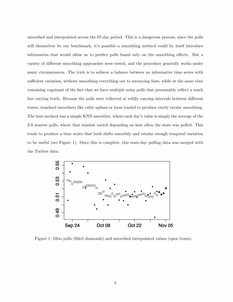
smoothed and interpolated across the 67-day period. This is a dangerous process, since the polls

will themselves be our benchmark; it’s possible a smoothing method could by itself introduce

information that would allow us to predict polls based only on the smoothing effects. But a

variety of different smoothing approaches were tested, and the procedure generally works under

many circumstances. The trick is to achieve a balance between an informative time series with

sufficient variation, without smoothing everything out to unvarying lines, while at the same time

remaining cognizant of the fact that we have multiple noisy polls that presumably reflect a much

less varying truth. Because the polls were collected at wildly varying intervals between different

states, standard smoothers like cubic splines or loess tended to produce overly erratic smoothing.

The best method was a simple KNN smoother, where each day’s value is simply the average of the

2-8 nearest polls, where that window varied depending on how often the state was polled. This

tends to produce a time series that both shifts smoothly and retains enough temporal variation

to be useful (see Figure 1). Once this is complete, this state-day polling data was merged with

the Twitter data.

Sep 24 Oct 08 Oct 22 Nov 05

0.49

0.51

0.53

0.55

textpoll$datev[textpoll$statev == k]

text

poll$

vsoi

nter

pol[t

extp

oll$

stat

ev =

= k]

Sep 24 Oct 08 Oct 22 Nov 05

0.49

0.51

0.53

0.55

textpoll$datev[textpoll$statev == k]

text

poll$

vote

shar

eo[te

xtpo

ll$st

atev

==

k]

Figure 1: Ohio polls (filled diamonds) and smoothed interpolated values (open boxes).

5

3 Estimation

At this point, we must think a bit more precisely about what we mean by “predicting” polls based

on Twitter data. There are many ways to construe this, the most challenging of which has not

yet been attempted: predicting polls multiple days in the future based on nothing but current

Twitter data.2 Rather, the question here is whether, given polling and Twitter data through day

t, one can use the Twitter data alone over subsequent days to accurately estimate the polling

results for those days. If we can do this, and we have established consistent patterns across

states, we can then use Twitter data to “predict” polling data for unpolled states or sub-state

regions, or unpolled days or sub-day time periods. As we will see, both geographic and temporal

out-of-sample prediction is quite possible, even down to fairly small regions or periods of time

since Twitter data are so plentiful and dense.

One key question will be for how long we can continue to predict polls based on that day’s

Twitter data without having to refit the model: that is, how long do specific word-poll associations

last before the topic of conversation has shifted so radically that the model must be updated and

fit anew? This issue will be returned to in the second part of the results section, but again to

preview, the unsurprising result is that the model fit rapidly declines as the issues and topics of

discussion change – but not so rapidly as to eliminate the utility of the model.

Fitting the model on m days in the past and predicting the state polls for the next day

generates far too few observations to properly test things: we would only have 24 observations

(the 24 states) to compare the text predictions with the polling data. Instead, a rolling window

approach is taken: fit on m days in the past, and predict the next day; then roll forward one day,

fit on the m previous days, and predict the next; and so forth. The result is a set of out-of-sample

predictions with both cross-sectional and temporal variation, which can measure how well this

approach works one day out of sample. This can be generalized, fitting the model on days t−m

2Papers that examine genuine prediction – or at least explore the lag between a Twitter-derived time seriesand the benchmark series – include Gruhl et al. (2005), Bollen, Mao & Zeng (2011), and O’Connor et al. (2010).However, tests of such predictions are difficult: false positives are easy without stringent tests on multiple timeseries with divergent trends, since sliding two time series against each other and picking the best lag is far fromout-of-sample.

6

through t and then using the text data for days t+ 1 through t+n to predict the polls for each of

those n days. As the window for t rolls forward, this process produces n sets of TSCS data, each

of which can be compared to the true TSCS poll data for those days, allowing us to estimate how

well the accuracy declines as we move steadily away from the period in which the model was fit.

To measure fit, rather than using mean square error – which lacks statistical tests or a

baseline for comparison – we leverage the fact that we are working in an established TSCS world,

and simply regress the text-predicted polls on the true polls, with well-established statistical tests.

But again, this raises the question of what exactly we wish to “predict.” If we directly compare

a set of predicted polls yit with the true polls yit in a pooled fashion, statistical significance may

be due to regional variation, temporal variation, or both. A statistically significant result, and

more importantly a large R2, would show that text-based predictions are feasible and (because it

is out-of-sample) not due to the sorts of spurious results to which wide data are prone. Assuming

the model was fit without any state-level effects, an out-of-sample prediction success would show

that other states, and presumably even smaller regions, could have their presidential polling levels

accurately predicted. Since local polling is often very hard to come by, this would be a very useful

tool in and of itself.

However, it would not be evidence that changes in polling over time could be predicted, so

it would be useless as a poll tracker or as a tool for picking up quick changes in vote intention

that might appear in the Twitter data before the traditional polls pick them up. For this higher

bar, we would need to be able to predict polling changes within states over time, a much harder

task. But the test of this is relatively straightforward: including fixed effects for each state at the

testing stage would absorb all the cross-sectional variation, allowing us to measure the within-state

prediction accuracy directly. And even here, there is yet a higher bar: since vote intention often

varies on the short scale against a background of slow changes (eg, Obama’s slowly declining polls

through much of the fall), it is easy to find statistical significance simply by merit of a predicted

time series that falls as the true time series also falls. However, standard solutions to this problem

from econometrics, such as time fixed effects, are not possible here, since we want to be able to

7

predict forward in time. Thus the high bar can be set by including a time trend, with the most

challenging measure of success being whether the textual data can help predict polls better than

state level fixed effects plus the time trend alone. But again, this is a high bar, and being able

to detect and extrapolate trends, not to mention predict regional variations, would be strong and

useful results in themselves – although as we will see, the model can do all three.

Given the various predictive tasks, the natural approach would be to fit the appropriate

model in-sample – pooled; with state fixed effects; with fixed effects and time trend – and then

predict vote share for each of the 24 states for days t+1 through t+n (and then repeat all this for

each rolling t). However, here we run into the second big-data challenge: we have 10,000 potential

predictor variables for each state and day. There are a wide host of machine learning methods

for dealing with high-dimensional models, but few are suited to TSCS data. One approach would

be to demean by state and/or detrend each in-sample TSCS dataset, pool the data, and employ

a standard tool such as Support Vector Machines, random forests, or shrinkage methods like

LASSO. But we can hew closer to the natural TSCS structure by estimating 10,000 separate

TSCS models and then employing techniques drawn from Bayesian model averaging (BMA) and

Bayesian shrinkage methods to combine them.

That is, one fits a set of k models as in equation (1), one model for each word k:

pjt = βj + γt+ βkwkjt + εkjt, for k in [1...10,000] (1)

This is the full model, with state fixed effects βj and a time trend effect τ , as well as a word

effect βk associated with word frequency wkjt. For each of these k models we can easily generate a

prediction pjt, and the BMA approach would average these predictions with weights in proportion

to the significance or precision of each model k. For instance, we might have

pjt =

K∑k=1

pjtk1

σβk

However, this is computationally costly, and more importantly, actually performs poorly due

8

to the imprecision of estimating σβk for all the myriad statistically insignificant words. Conversely,

we might employ shrinkage methods, shrinking each individual pjtk toward the group mean, again

with a weighting such as σβk . But a more efficient (and more effective, at least in this case)

approach is simply to assign some cutoff significance threshold below which no prediction pjtk

will be included; this leaves a parameter to be estimated, but that is no different from shrinkage

methods, which generally have at least one free parameter associated with the weight assigned

to the group mean.3 And finally, since averaging the fixed effect and trend contribution from

each model just adds noise, we employ in the prediction stage simply the state means as the fixed

effects βj and the time trend τ from the fixed-effect estimate without the words. Thus our final

prediction is

pjt = βj + τ t+∑

k∈{λ(σβk )}

βkwkjt (2)

where the coefficients βk have been ranked by their associated p-value, only those under

some threshold λ retained, and then averaged without further shrinkage or weighting.

Finally, to test these text-based poll predictions, we simply return to the original TSCS

model, and estimate

pjt = β′j + γpjt + εjt (3)

for the out-of-sample period of time. Again, we will explore variants on these models – without

fixed effects or time trends – but the essential structure is the same. Ultimately, we want to know

whether the coefficient γ is significant, and what proportion of the variation of pjt we can explain

with the pjt that we have generated from the text – in the pooled case, in the fixed-effects case,

and in the difficult time-trend case.

3Futhermore, in practice few of the variables in shrinkage methods like LASSO are actually shrunk very much;in general, for a given shrinkage level, one finds two sets of variables – those that are unshrunk and those that areshrunk all the way down to zero, with only a few in between. Thus the cutoff approach is mainly just an expeditedversion of LASSO or any other shrinkage method.

9

4 Results

The results of the various models are summarized in Table 2. There are five distinct models, each

of which describe the factors that went into the prediction estimation, not the prediction test. In

all but the first model, the prediction test is the same, exactly as in Equation 3. In all cases, the

full dataset is the 9 weeks leading up to the election. The in-sample is all 24 states for 21 days,4

and the out-sample is the same states for the next day; to generate the 42 days of predictions,

we roll the 21-day window forward one day at a time, fit it, predict the next day using that day’s

textual data, and roll it forward again. The end result is a 24 state x 42 day TSCS dataset to

test the predictions against the true polls.

Table 1: Fit between prediction and truth forrolling one-day-ahead models.

M1 M2 M3 M4 M5

Twitter text x - x - xState fixed effects - x x x xTime trend - - - x x

R2 Pooled 0.74 0.98 0.98 0.98 0.98R2 Within 0 0.18 0.25 0.37 0.40

In Model 1, the text coefficients are estimated as Equation 1, except without state fixed

effects or time trend; the predictions are averaged as Equation 2, again without the fixed effects

or time trend; and then they are tested as in Equation 3 – again, without the βj . Though

a simple pooled estimation and test, the model is an important one: it establishes whether

the textual data can predict the polling data out-of-sample, which is already a more stringent

standard than most Twitter and other textual approaches that supposedly discover correlates

between substantively interesting outcomes (such as vote intention) and speech variation. And

indeed this pooled prediction works quite well: the γ coefficient in equation 3 is highly significant

4Brief testing showed that a 21-day window worked best, though little better than a 14- or 28-day window.

10

(p << 1−10), and as can been seen in Table 1, the pooled R2 is quite high. We are evidently able

to differentiate the level of Obama support in various regions with solid accuracy, giving hope

that this approach can be used to estimate vote intention in other states and the myriad smaller

regions that are often so poorly polled – but nevertheless heavily represented on Twitter. No

doubt this model would be boosted considerably by including as controls the various demographic

characteristics we know about states and (when it comes to prediction) smaller regions, and since

some states are predicted better than others, we might also like to explore what the sources of

that variation are. But clearly this is a good start.

That said, the within-state accuracy is very low: the within R2 (for instance, when including

state fixed effects in the testing stage, as in Equation 3) is little better than 0. Insofar as we are

interested in polling changes over time, and not just across regions, we need to be able to match

polling shifts within states, and not just variation across them. Indeed, if we include only fixed

effects – ie, we use the state means for our prediction in Equation 3, and nothing else – we achieve

a pooled R2 of 0.98 and a within R2 of 0.18 (Model 2). This shows that, unsurprisingly, we

can do a pretty good job predicting a state’s polling level in the future but simply extrapolating

its polling level in the past. However, this is useless in a predictive sense, inasmuch as it of

course doesn’t allow us to estimate poll levels for geographical regions (states, districts) for which

we do not already have polling data. But it does set the benchmark for intra-state accuracy:

0.18 is relatively high because, recall, we are not just taking the state poll levels at time t and

extrapolating forward until the end; rather, as each state changes, its past mean in the 21-day

window slowly shifts, giving a fairly accurate prediction for the next day, and setting a high bar

for the textual data.

Model 3 tests what the textual data can add with this much higher bar, looking only at the

tough task of explaining within-state – ie, temporal – variation. Here we estimate the model as

in Equation 1 without the time trend, and we predict similarly with Equations 2 and 3.5 The

5More precisely, for each prediction Models 2 through 5, the various factors – fixed effects, time trend, and textprediction – are combined in a weighted fashion, with each of the three weight parameters estimated ahead of timeusing a subsample. Testing suggests that predictive accuracy does not vary very much under a broad set of weights,suggesting that no over-fitting is occurring. There is also a fourth parameter to estimate, the cutoff threshold λ –

11

improvement over the baseline, while not enormous, is quite significant, both statistically and

substantively. It shows that text can predict temporal as well as geographical variation, allowing

us to extrapolate forward in time as well as into smaller time periods on scales less than a day.

While the accuracy could certainly be improved upon, this is a very stringent out-of-sample test,

with the net fully up.

A skeptic, however, might wonder how much of this accuracy is due simply to picking out

words that match some general polling trend over the 21-day window, and simply extrapolating

forward from that. Of course, the model does not knowingly do this: for this extrapolation to

work, those words must in fact continue to decline in tandem with the polling. If the polls simply

shifted in one direction over the course of this time, then we would have serious grounds to worry

– but as is well known (and we will see briefly), the polls in fact declined for Obama for a while

during this period, and then slowly recovered during the last weeks of the campaign. To test the

power of the simple time-trend extrapolation, we can include the time trend in Equation 1, and

indeed this does do better than the fixed-effects extrapolation of Model 2, as well as the text-based

extrapolation of Model 3 (within R2 = 0.25). But as with Model 2 vs Model 1, this is cheating

somewhat, since we know we are working with data that do not change wildly over our time

period. But once again, if we add the textual data back in (controlling for the time trend when

making our βk estimates in Equation 1), we still can improve upon this fixed-effects + time-trend

benchmark, albeit not hugely (though the difference is highly statistically significant). At this

point, the added benefit is coming only from the evanescent, intra-state changes in polling and

speech over periods of time less than three weeks, lending support to the idea that this approach

can be used to potentially predict polling changes on very short time scales, possibly even in

real-time during periods of heavy political interest such as speeches or debates. Once again, there

remains much room for improvement, but this high bar shows that the approach does indeed

work, with a pooled R2 of more than 0.98 and a final within R2 of 0.4.

ie, the p-value above which we do not include those word coefficients βk. This of course leads to a tradeoff betweentype 1 and type 2 errors, and for most models the best threshold was on the order of 0.001. With 10,000 estimands,we would expect a small number of false positives with that threshold, but generally that cutoff retains between100 and 500 words per t, so the vast majority are unlikely to be spurious.

12

Two obvious sources of improvement would be exploring the lag between Twitter and the

polls more closely – indeed, it is quite possible that the former could lead the latter, leading to

genuine predictive power – and incorporating the one-day-ahead errors as the window rolls forward

to improve the model above and beyond simply refitting it. One additional interesting source of

increased accuracy could be to employ a model with text coefficients that vary by state, βjk;

this would presumably boost the predictive accuracy and the within-R2, although with 240,000

parameters to estimate one would have to make heavy use of shrinkage to overcome the increased

noise of the within-state estimation. Partially as a result of the shared βk across states, the time

trends within each state are currently relatively similar, correlating at around the 0.8 or 0.9 level

– although this could also simply reflect the fact that polls tend to move nationally rather than

varying in their state variation. Nevertheless, some states are in fact predicted better than others,

as can be seen in Table 2, which shows individual state regressions using the predictions from the

pooled Model 1.

An example from an important and reasonably well-predicted state, Ohio, is shown in Figure

2, where black diamonds are the predicted poll levels and the squares are the true (filled squares

are actual polls, open squares are interpolated polls; red and blue lines are lowess lines simply for

illustration). The match is by no means perfect, but the predicted series shows the all-important

dip in early October (the notorious first debate), though not nearly as severely as in the actual

polling data (although these are still relatively sparse polls, and may themselves exaggerate the

dip, as Obama supporters fervently hoped at the time). Both series then slowly recover, although

the text-based measure begins to recover more immediately. But this predicted sequence is so

smooth (no smoothing has been applied to the point measures) and based on such dense data

(millions of word instances a day) that it is quite possible that this actually more accurately

reflects opinion that the erratic and intermittent polls themselves.

One final important question raised earlier is how well this fit between text and polls lasts

into the future. That is, how often do we have to refit a model – requiring fresh, or at least

extrapolated, polling data – as actual time rolls along? Figure 3 shows that as we venture more

13

Table 2: P-values from regressions of true poll values againsttext-predict predicted values by each state individually, fromthe pooled model 1.

arizona 4.33e−04∗∗∗

california 0.09†

colorado 1.46e−07∗∗∗

connecticut 8.96e−07∗∗∗

florida 5.47e−03∗∗∗

indiana 0.17iowa 0.25maine 6.30e−04∗∗∗

massachusetts 0.05∗

michigan 0.74minnesota 0.37missouri 0.60montana 1.82e−03∗∗

nevada 0.08†

new hampshire 0.03∗

new jersey 0.95new mexico 6.21e−03∗∗

new york 0.26north carolina 3.81e−05∗∗∗

ohio 9.35e−3∗∗

pennsylvania 0.09†

virginia 1.85e−04∗∗∗

washington 0.37wisconsin 1.51e−04∗∗∗

† significant at p < .10; ∗p < .05; ∗∗p < .01; ∗∗∗p < .001

than 1 day away from the fitting, the accuracy drops steeply. Figure 3 shows two model groups,

with slightly different parameters.6 The triangle and x (green and purple) correspond to Models

5 and 4 respectively, which were maximized for one-day-ahead prediction. The diamond and

square (blue and red) are exactly as in Models 5 and 4, but the weight parameters are slightly

different, having been maximized for the total (within) R2 over these four days. In both cases,

the advantage of the text over the time trend alone has disappeared by day 4, suggesting that

the words and topics of conversations shift very rapidly, and must be updated frequently. As

6See footnote 5.

14

Sep 24 Oct 01 Oct 08 Oct 15 Oct 22 Oct 29 Nov 05

0.51

00.

520

0.53

0

textpoll$datev[textpoll$statev == k]

text

poll$

vsoi

nter

pol[t

extp

oll$

stat

ev =

= k]

Sep 24 Oct 01 Oct 08 Oct 15 Oct 22 Oct 29 Nov 05

0.51

00.

520

0.53

0

textpoll$datev[textpoll$statev == k]

0.51

52 +

0.0

0757

* te

xtpo

ll$te

xtvs

o[te

xtpo

ll$st

atev

==

k]

Sep 24 Oct 01 Oct 08 Oct 15 Oct 22 Oct 29 Nov 05

0.51

00.

520

0.53

0

textpoll$datev[textpoll$statev == k]

text

poll$

vote

shar

eo[te

xtpo

ll$st

atev

==

k]

Figure 2: Predicted and actual polling for Ohio. Filled squares: actual poll values; opensquares, interpolated and smoothed values; black diamonds, text-based predictions. Blueand red lines are Loess fitted curves for true and predicted polls, respectively, and aremerely descriptive here.

in the first two models, we can somewhat boost the staying power at the cost of the short-term

prediction accuracy. The best accuracy comes from a mixture: using Model 5 for day 1, the

reweighted Model 5 for days 2 and 3, and defaulting back to the simple time trend for any further

prediction if the text model cannot be refit and updated on newer topics.

It should also be said that the rate of staleness does depend on the period under examination.

The previous figure examined only 4 days into the future, because anything more would cause

us to lose fitting data (since the rolling window t can only begin 21 days after the start of the

data and must end the 4 days before the end of the data). But we can temporarily accept that

drawback, and examine how the model stales more than 4 days into the future. Figure 4 shows 21

days, but at the cost of only retaining 25 testing days instead of the previous 42. The result is that

the overall accuracy is higher, although the advantage of the text over the time trend alone for

this period is less. This is due to the fact that during these 25 days, Obama’s polling was steadily

declining, so the trend alone happens to do quite well. But even so, we can see that the accuracy

trails off again, albeit less steeply. Notable as well is the fact that the Model 5 maximized for one-

day-ahead accuracy has a sudden drop off at day 7 (green, triangle), illustrating what the 4-day

model missed: that Twitter speech clearly follows a weekly cycle, with topics not just changing

15

!"#$%

!"&%

!"&$%

!"'%

!"'$%

!"(%

#% &% '% (%

!"#$%&

'()'*+$

,-./$'*(0$12(234$/'*54$67*8$

)*+,-%./,%012%3*3.4%

5612%*/47%3*3.4%

)*+,-%./,%012%8+-3%,.7%

5612%*/47%8+-3%,.7%

Figure 3: Accuracy of predicted polls based on an increasingly old model. The latter twoare as in Models 5 and 4, which were optimized for one-day-ahead accuracy (triangle andx), whereas the first two are Models 5 and 4 that have been optimized over the sum of R2

over all four days (diamond and square). Note that in both cases, the advantage of thetext over the time trend alone disappears by day 4.

steadily over time, but changing quite significantly on a weekly basis. Nevertheless, despite the

evanescence of Twitter chatter, it remains constant long enough for us to be able to extrapolate

polling to different states and into the future, and potentially into smaller regions or time periods.

We finish by looking at the words that make this work.

5 Textual content

Having established there are strong, predictively useful correlations between what people are

tweeting and what the state-level (and not just Twitter user) vote intentions are, we can also

learn about how these vote intentions relate to specific elements of the Twitter speech. This

goes well beyond merely describing what words or topics users employ to speak about Obama

or Romney, or even what words Obama or Romney supporters employ. Instead, we can discern

here the words that actually track vote intention: words that surge up or down with pro- or

16

!"!!!#

!"!$!#

!"%!!#

!"%$!#

!"&!!#

!"&$!#

!"'!!#

!"'$!#

!"(!!#

!"($!#

!# $# %!# %$# &!#

!"#$%&

'()'*+$

,-./$'*(0$12(234$/'*54$67*8$

)*+,-#./,#012#3*3.4#

5612#*/47#3*3.4#

)*+,-#./,#012#8+-3#,.7#

5612#*/47#8+-3#,.7#

Figure 4: Accuracy of predicted polls based on an increasingly old model. The lattertwo are as in Models 5 and 4 (triangle and x), which were optimized for one-day-aheadaccuracy, whereas the first two are Models 5 and 4 have been optimized over the sum ofR2 over all 21 days (diamond and square).

anti-Obama sentiment, and reflect (or perhaps even cause) changes in intended political behavior.

Before turning to the entire corpus of words, though, it is worthwhile to examine the two most

crucial words in the corpus, which were in large part constitutive of it: “obama” and “romney”.

Figures 4 and 5 show the variation in the frequency of these words plotted against the Obama

vote share, pooled across all states and times. What is notable here is the strikingly different

relationships for these two words: up through about 52% Obama intended vote, both increase

(already an asymmetry), and after about 52% both decline – reasonably enough, as the state

is becoming uncompetitive. However, beyond that point, “obama” mentions are almost entirely

17

flat, whereas mentions of “romney” continue to increase linearly with increasing Obama intended

vote. This suggests that the use of “obama” is much more tied to pragmatic questions of victory,

whereas mentions of “romney” may depend more on the sheer number of Democrats (or how

embattled the Republicans feel; we of course do not know the parties of those mentioning these

names). This also suggests that a more sophisticated model of the relationship between polls and

text should perhaps include quadratic terms, since the “obama” sequence using the pooled data

shows almost no linear significance, entirely due to the fact that the relationship is quadratic (and

very strong).

0.40 0.45 0.50 0.55 0.60 0.650.000

0.010

0.020

0.030

polltwit$vsointerpol

polltwit$romney

Figure 5: Frequency of the appearance of the word “romney” by intended Obama voteshare (units: state-days).

0.40 0.45 0.50 0.55 0.60 0.65

0.005

0.015

0.025

polltwit$vsointerpol

polltwit$obam

a

Figure 6: Frequency of the appearance of the word “obama” by intended Obama voteshare (units: state-days).

18

But which words are most closely associated with changes in pro-Obama or pro-Romney

vote intention? To answer this, we once again have to specify which model we are interested in:

Model 1 (pooled), Model 3 (with fixed effects), or Model 5 (with fixed effects and a time trend).

Each set of words captures different types of variation in vote intention: across regions, general

trends, and evanescent shifts, respectively. Tables 3 through 5 show the words most associated

with pro-Obama and pro-Romney vote intention in the pooled, fixed-effect, and time-controlled

models. The results show an interesting blend of confirming what we might expect, and suggesting

new ideas and topics than might have been reflecting or even driving changes in vote intention.

As we might expect, Table 3 exhibits mainly words that are associated with regional varia-

tion: New York and Massachusetts for Obama, Missouri, Montana, and Indiana for Romney. If

the significant words were only such state names, they would of course be useless for extrapolation

to any other regions, but of course there is much more than this. Romney in particular is rich in

words both suggestive and slightly opaque to those who do not closely follow the insular world of

right-wing social media – as exhibited, if nothing else, but the fact that rt (retweet) is the term

most tightly associated with pro-Romney vote intention in the entire corpus. This is certainly in

keeping with past results suggesting that the Republican social-media world is much more unified

and self-echoing than the Democratic.

Table 3: Words associated with pro-Romney and pro-Obama poll shifts, pooled model.

Pro-Obama

#ucwradio, #ny, #politics, ny, #hot, brooklyn,reuters, #business, ma, boston, cuomo, #google,york, #hitechcj, #socialmedia, #nytimes, scott,massachusetts, elizabeth, #boston

Pro-Romney

rt, socialists, indiana, #ccot, #dloesch, #ocra,montana, #dems, #insen, #patdollard, #the-blaze, donnelly, #townhallcom, #jjauthor, #mo,mo, missouri, #lnyhbt, o, bjp

19

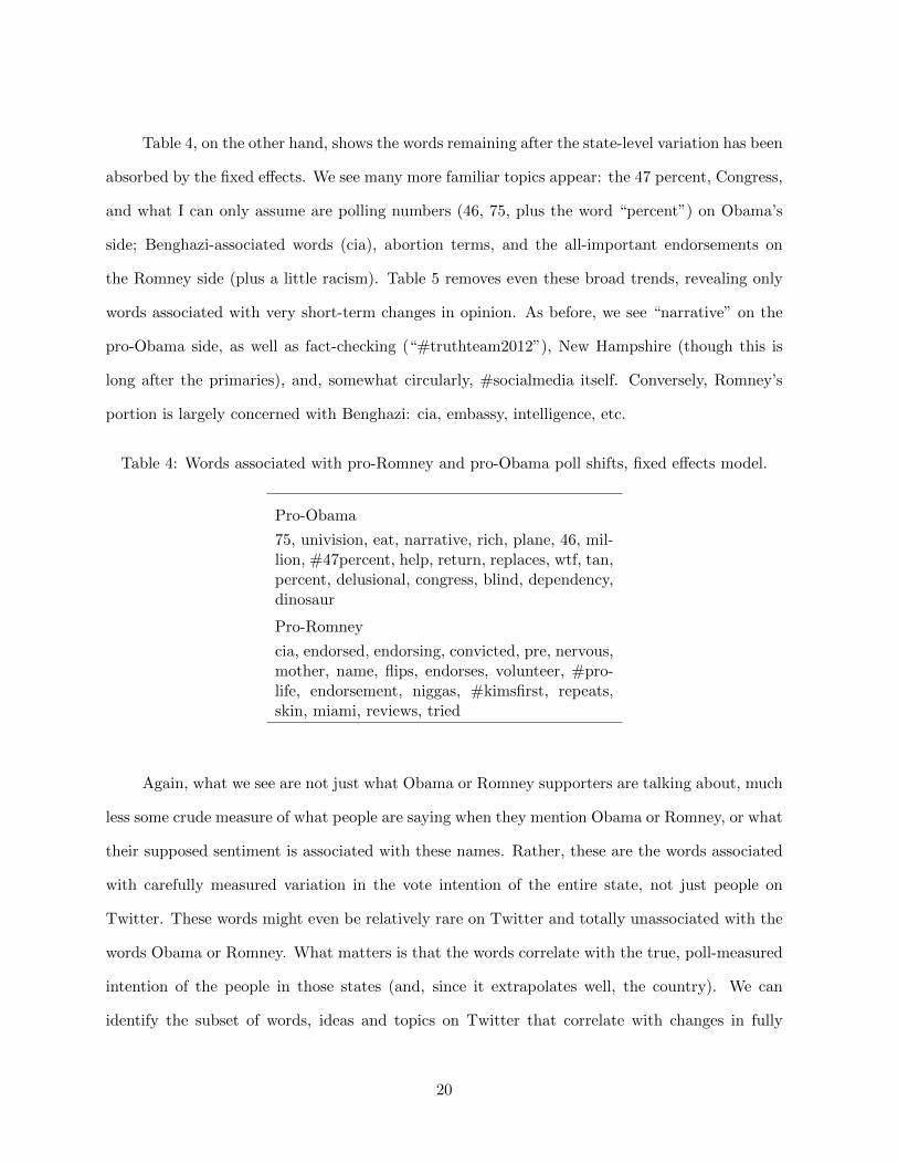
Table 4, on the other hand, shows the words remaining after the state-level variation has been

absorbed by the fixed effects. We see many more familiar topics appear: the 47 percent, Congress,

and what I can only assume are polling numbers (46, 75, plus the word “percent”) on Obama’s

side; Benghazi-associated words (cia), abortion terms, and the all-important endorsements on

the Romney side (plus a little racism). Table 5 removes even these broad trends, revealing only

words associated with very short-term changes in opinion. As before, we see “narrative” on the

pro-Obama side, as well as fact-checking (“#truthteam2012”), New Hampshire (though this is

long after the primaries), and, somewhat circularly, #socialmedia itself. Conversely, Romney’s

portion is largely concerned with Benghazi: cia, embassy, intelligence, etc.

Table 4: Words associated with pro-Romney and pro-Obama poll shifts, fixed effects model.

Pro-Obama

75, univision, eat, narrative, rich, plane, 46, mil-lion, #47percent, help, return, replaces, wtf, tan,percent, delusional, congress, blind, dependency,dinosaur

Pro-Romney

cia, endorsed, endorsing, convicted, pre, nervous,mother, name, flips, endorses, volunteer, #pro-life, endorsement, niggas, #kimsfirst, repeats,skin, miami, reviews, tried

Again, what we see are not just what Obama or Romney supporters are talking about, much

less some crude measure of what people are saying when they mention Obama or Romney, or what

their supposed sentiment is associated with these names. Rather, these are the words associated

with carefully measured variation in the vote intention of the entire state, not just people on

Twitter. These words might even be relatively rare on Twitter and totally unassociated with the

words Obama or Romney. What matters is that the words correlate with the true, poll-measured

intention of the people in those states (and, since it extrapolates well, the country). We can

identify the subset of words, ideas and topics on Twitter that correlate with changes in fully

20

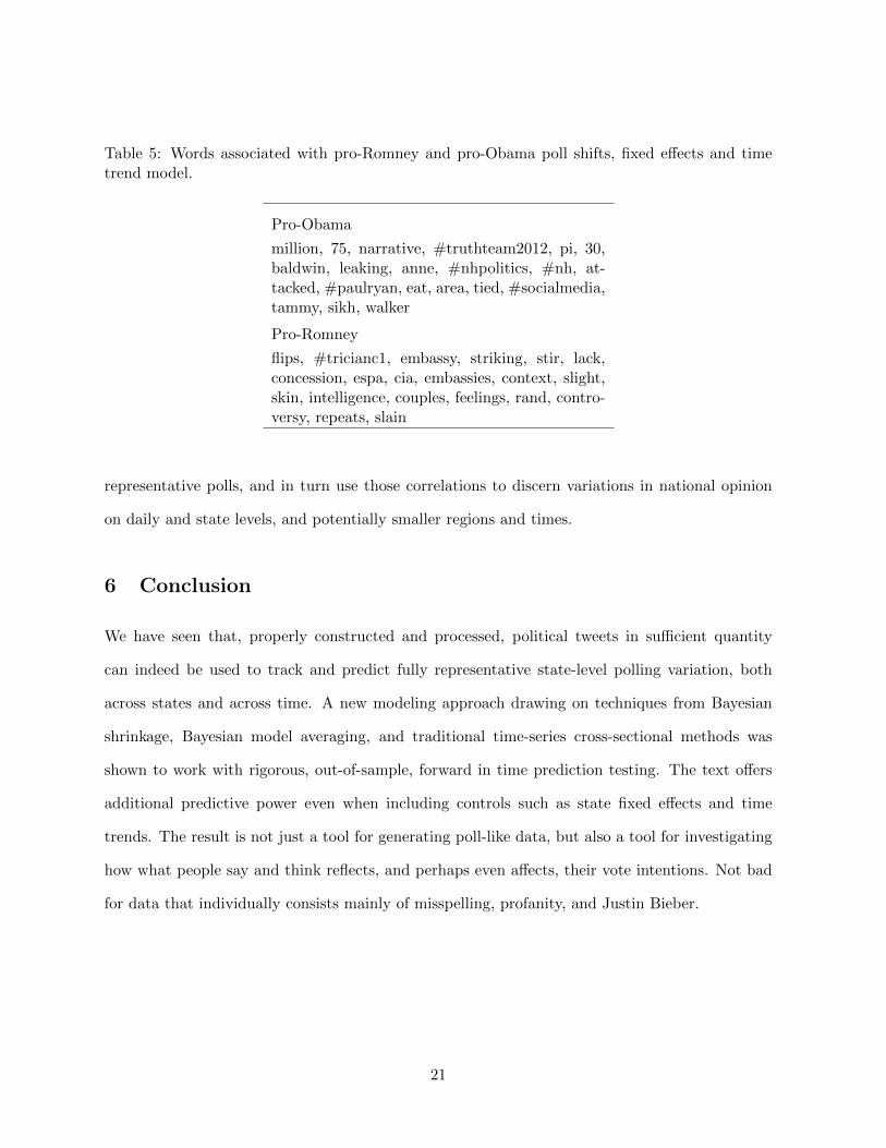
Table 5: Words associated with pro-Romney and pro-Obama poll shifts, fixed effects and timetrend model.

Pro-Obama

million, 75, narrative, #truthteam2012, pi, 30,baldwin, leaking, anne, #nhpolitics, #nh, at-tacked, #paulryan, eat, area, tied, #socialmedia,tammy, sikh, walker

Pro-Romney

flips, #tricianc1, embassy, striking, stir, lack,concession, espa, cia, embassies, context, slight,skin, intelligence, couples, feelings, rand, contro-versy, repeats, slain

representative polls, and in turn use those correlations to discern variations in national opinion

on daily and state levels, and potentially smaller regions and times.

6 Conclusion

We have seen that, properly constructed and processed, political tweets in sufficient quantity

can indeed be used to track and predict fully representative state-level polling variation, both

across states and across time. A new modeling approach drawing on techniques from Bayesian

shrinkage, Bayesian model averaging, and traditional time-series cross-sectional methods was

shown to work with rigorous, out-of-sample, forward in time prediction testing. The text offers

additional predictive power even when including controls such as state fixed effects and time

trends. The result is not just a tool for generating poll-like data, but also a tool for investigating

how what people say and think reflects, and perhaps even affects, their vote intentions. Not bad

for data that individually consists mainly of misspelling, profanity, and Justin Bieber.

21

References

Asur, Sitaram & Bernardo A Huberman. 2010. Predicting the future with social media. In Web In-telligence and Intelligent Agent Technology (WI-IAT), 2010 IEEE/WIC/ACM InternationalConference on. Vol. 1 IEEE pp. 492–499.

Bollen, Johan, Huina Mao & Xiaojun Zeng. 2011. “Twitter mood predicts the stock market.”Journal of Computational Science 2(1):1–8.

Chung, Jessica Elan & Eni Mustafaraj. 2011. Can collective sentiment expressed on twitter predictpolitical elections? In AAAI.

Gaurav, Manish, Amit Srivastava, Anoop Kumar & Scott Miller. 2013. Leveraging candidatepopularity on Twitter to predict election outcome. In Proceedings of the 7th Workshop onSocial Network Mining and Analysis. ACM p. 7.

Gayo-Avello, Daniel, Panagiotis Takis Metaxas & Eni Mustafaraj. 2011. Limits of electoral pre-dictions using twitter. In ICWSM.

Gruhl, Daniel, Ramanathan Guha, Ravi Kumar, Jasmine Novak & Andrew Tomkins. 2005. Thepredictive power of online chatter. In Proceedings of the eleventh ACM SIGKDD internationalconference on Knowledge discovery in data mining. ACM pp. 78–87.

Huberty, Mark. 2013. “Multi-cycle forecasting of Congressional elections with social media.”.

Jungherr, Andreas, Pascal Jurgens & Harald Schoen. 2012. “Why the pirate party won the germanelection of 2009 or the trouble with predictions: A response to tumasjan, a., sprenger, to,sander, pg, & welpe, im “predicting elections with twitter: What 140 characters reveal aboutpolitical sentiment”.” Social Science Computer Review 30(2):229–234.

O’Connor, Brendan, Ramnath Balasubramanyan, Bryan R Routledge & Noah A Smith. 2010.“From Tweets to Polls: Linking Text Sentiment to Public Opinion Time Series.” ICWSM11:122–129.

Sang, Erik Tjong Kim & Johan Bos. 2012. Predicting the 2011 dutch senate election results withtwitter. In Proceedings of the Workshop on Semantic Analysis in Social Media. Associationfor Computational Linguistics pp. 53–60.

Stewart, Justin, Homer Strong, Jeffery Parker & Mark A Bedau. 2012. Twitter keyword volume,current spending, and weekday spending norms predict consumer spending. In Data MiningWorkshops (ICDMW), 2012 IEEE 12th International Conference on. IEEE pp. 747–753.

Tumasjan, Andranik, Timm Oliver Sprenger, Philipp G Sandner & Isabell M Welpe. 2010. “Pre-dicting Elections with Twitter: What 140 Characters Reveal about Political Sentiment.”ICWSM 10:178–185.

22