Predictability of Seasonal Sahel Rainfall Using GCMs …ousmane/print/pub/Ndiayeetal11_JClim.pdf ·...

Predictability of Seasonal Sahel Rainfall Using GCMs and Lead-TimeImprovements Through the Use of a Coupled Model

OUSMANE NDIAYE

Department of Earth and Environmental Sciences, Columbia University, New York, New York,

and Agence Nationale de la Meteorologie du Senegal, Dakar, Senegal

M. NEIL WARD

International Research Institute for Climate and Society, Columbia University, Palisades, New York

WASSILA M. THIAW

NOAA/Climate Prediction Center, Camp Springs, Maryland

(Manuscript received 8 December 2009, in final form 18 November 2010)

ABSTRACT

The ability of several atmosphere-only and coupled ocean–atmosphere general circulation models

(AGCMs and CGCMs, respectively) is explored for the prediction of seasonal July–September (JAS) Sahel

rainfall. The AGCMs driven with observed sea surface temperature (SST) over the period 1968–2001 confirm

the poor ability of such models to represent interannual Sahel rainfall variability. However, using a model

output statistics (MOS) approach with the predicted low-level wind field over the tropical Atlantic and

western part of West Africa yields good Sahel rainfall skill for all models. Skill is mostly captured in the

leading empirical orthogonal function (EOF1), representing large-scale fluctuation in the regional circula-

tion system over the tropical Atlantic. This finding has operational significance for the utility of AGCMs

for short lead-time prediction based on persistence of June SST information; however, studies have shown

that for longer lead-time forecasts, there is substantial loss of skill, relative to that achieved using the observed

JAS SST.

The potential of CGCMs is therefore explored for extending the lead time of Sahel rainfall predictions.

Some of the models studied, when initialized using April information, show potential to at least match the

levels of skill achievable from assuming persistence of April SST. One model [NCEP Climate Forecasting

System (CFS)] was found to be particularly promising. Diagnosis of the hindcasts available for the CFS (from

lead times up to six months for 1981–2008) suggests that, especially by applying the same MOS approach, skill

is achieved through capturing interannual variations in Sahel rainfall (primarily related to El Nino–Southern

Oscillation in the period of study), as well as the upward trend in Sahel rainfall that is observed over 1981–

2008, which has been accompanied by a relative warming in the North Atlantic compared to the South At-

lantic. At lead times up to six months (initialized forecasts in December), skill levels are maintained with the

correlation between predicted and observed Sahel rainfall at approximately r 5 0.6. While such skill levels at

these long lead times are notably higher than previously achieved, further experiments, such as over the same

period and with comparable AGCMs, are required for definitive attribution of the advance to the use of

a coupled ocean–atmosphere modeling approach. Nonetheless, the detrended skill achieved here by the

January–March initializations (r 5 0.33) must require an approach that captures the evolution of the key

ocean–atmosphere anomalies from boreal winter to boreal summer, and approaches that draw on persistence

in ocean conditions have not previously been successful.

Corresponding author address: Ousmane Ndiaye, 133 Monell Building, LDEO Campus, Palisades, NY 10964.

E-mail: [email protected]

1 APRIL 2011 N D I A Y E E T A L . 1931

DOI: 10.1175/2010JCLI3557.1

� 2011 American Meteorological Society

1. Introduction

The climatology of the Sahel region is dominated by

dry conditions for most of the year, with a single peak in

rainfall during boreal summer. It is well established that

there is a strong relationship between this July–September

(JAS) seasonal Sahel rainfall and near-global patterns of

sea surface temperature (SST; Lamb 1978a,b; Folland

et al. 1986; Wolter 1989; Hastenrath 1990; Rowell et al.

1995; Fontaine and Janicot 1996; Ward 1998; Thiaw et al.

1999; Giannini et al. 2003). This now constitutes the basis

of operational short lead-time seasonal forecasting over

West Africa (e.g., ACMAD 1998).

However, many atmospheric general circulation models

(AGCMs) when forced with the observed SST continue

to have difficulty in simulating the observed variations

of seasonal rainfall over the Sahel. This was noted in

many early simulations (Sud and Lau 1996) and is gen-

erally noted to still be the case today (e.g., Lau et al.

2006; Scaife et al. 2009). This is despite the early re-

alization that SST in all ocean basins could potentially

impact Sahel rainfall in an AGCM (Palmer 1986).

The approach taken in Ndiaye et al. (2009), to address

the problem with AGCM simulations of Sahel rainfall,

was to focus on indices of the regional circulation system

predicted by the AGCM (ECHAM4.5) and to use the

indices in a model output statistics (MOS) to predict

Sahel rainfall. The ECHAM4.5 AGCM is typical in its

poor level of skill for Sahel rainfall; however, using the

low-level wind field over the tropical Atlantic and west-

ern part of West Africa, a level of skill in predicting Sahel

rainfall is achieved that is comparable with the small

number of AGCMs that have been able to successfully

represent the impact of SST directly on Sahel rainfall

(e.g., Giannini et al. 2003). The use of the tropical At-

lantic wind fields in this way is consistent with diagnostics

studies (e.g., Lamb 1978a,b; Hastenrath 1990; Janicot

1992) that have shown how, in the observed climate,

the tropical Atlantic wind field is strongly tied to Sahel

rainfall variations.

For seasonal prediction with an AGCM, the model

must be driven with a predicted field of SST. A simple

approach is to assume persistence of SST anomalies

when generating SST boundary conditions for AGCM

forecast runs. For AGCM forecasts of Sahel rainfall, the

published literature contains no clear systematic improve-

ments on this approach. Applying the persistence ap-

proach, although June SST showed good skill in Ndiaye

et al. (2009), prediction skill from May and April SST

was substantially reduced, even after applying the MOS

system.

A complicating factor for seasonal prediction of Sahel

rainfall is the strong presence of multidecadal variability

as well as strong interannual variations of rainfall

(Nicholson 1980). The post-1970 period is recognized as

being, on average, relatively dry compared to the 1950–70

period, with some amelioration of conditions having oc-

curred in recent years. The SST patterns associated with

the multidecadal and interannual Sahel rainfall fluctu-

ations have substantial differences (Ward 1998). On the

interannual time scale, variations in the tropical Atlan-

tic, and variations throughout the tropics associated with

El Nino–Southern Oscillation (ENSO), tend to be dom-

inant. On the multidecadal time scale, large-scale con-

trasts of warming/cooling in the North Atlantic compared

to the South Atlantic and Indian Ocean have been found

to accompany low-frequency (time scale greater than

about 10 yr) Sahel rainfall fluctuations throughout the

twentieth century (Folland et al. 1991; Giannini et al.

2003; Zhang and Delworth 2006; Knight et al. 2006).

There has emerged contrasting properties of seasonal

prediction skill associated with the two time scales. Skill

in terms of correlation between predicted and observed

rainfall is generally less if there is less low-frequency

variance in the analysis period. For example, achievable

skill is less for the post-1970 period, as compared to the

post-1950 period. Furthermore, to date, there is very

limited lead time for forecasts of the interannual time-

scale seasonal rainfall variations, for which skill has been

largely confined to very short lead times (zero to one-

month lead). This is found in statistical seasonal forecast

schemes that use SST (Ward 1998) and in AGCMs driven

with persisted SST (Ndiaye et al. 2009).

The period of AGCM forecasts available to the sci-

entific community for study is, for practical reasons,

mostly concentrated in the post-1970 period. This period

is known to be one in which Sahel rainfall has shown

a strong correlation with tropical Pacific SSTs related to

ENSO (Semazzi et al. 1988; Janicot et al. 1996, 2001;

Ndiaye et al. 2009). Indeed, the abrupt skill drop be-

tween May and June was found in Ndiaye et al. (2009) to

be primarily related to the SST evolution over the east-

ern equatorial Pacific (Nino-3 region), although signifi-

cant changes in the tropical Atlantic and tropical Indian

Ocean were also noted. This drop of skill limits the utility

of the seasonal climate forecast. The short lead time of

the forecast is a constraint on the timely dissemination

of climate information to potential users to better plan

their climate-related activities (such as farming, water

management, and malaria disease control). The longer

the lead time, the better it is for the users in this region of

the world where resources are very limited and need to

be managed with care.

The objectives of the current study build on the above

findings in two primary ways. First, we aim to generalize

the MOS approach using the tropical Atlantic circulation,

1932 J O U R N A L O F C L I M A T E VOLUME 24

noting the single-model result with the ECHAM4.5

AGCM found in Ndiaye et al. (2009), and exploring

its applicability generally across AGCMs. If a positive

result can be achieved, this builds confidence in the

use of AGCMs for Sahel rainfall prediction. A positive

result may also guide analyses for improvements in the

representation of Sahel precipitation itself in AGCMs.

Second, the study considers the ability of coupled ocean–

atmosphere general circulation models (CGCMs) for

increasing the lead time of skillful Sahel rainfall pre-

dictions. In the CGCMs, analysis is made of both model

precipitation and the potential for using the predicted

regional circulation system as a MOS predictor for the

rainfall. For the most promising coupled model, diagnosis

of the teleconnections, from the tropical Pacific and in

the Atlantic, is undertaken to reinforce conclusions about

the ability of the model to project forward the coupled

system and anticipate the key tropical Atlantic wind fields

for specifying Sahel rainfall. Furthermore, since the pe-

riod of model hindcasts covers 1981–2008, the study

considers the extent to which the model skill is derived

from an ability to track the recent recovery in Sahel rains

(low-frequency component of rainfall), as well as the

ability to capture the interannnual variations in rainfall

such as associated with ENSO. Since the CGCMs stud-

ied do not have directly comparable AGCM prediction

experiments, interpretation on the source of any im-

provements in skill require an element of diagnostic

interpretation. For example, it can be argued that ad-

vances in skill achieved by a CGCM may be attribut-

able solely to the atmospheric component of the model

or to the exact period of analysis. Therefore, diagnostics

on the ability to represent evolution of coupled ocean–

atmosphere phenomena previously not represented in

AGCM prediction experiments and assessment of the

characteristics of trend and interannual components

separately all add to the insights that can be gained from

the experiments analyzed here.

We first describe the data and methods used (section

2). The robustness of the MOS approach for Sahel sea-

sonal rainfall prediction is explored in section 3, evalu-

ating the performance of eight AGCMs driven with

observed SST. In section 4, the predictability of Sahel

rainfall from April–May initial conditions is explored in

coupled CGCMs. In section 5, the most promising cou-

pled model [the Climate Forecasting System (CFS)]

is evaluated for longer-lead predictions, with initial-

izations at incrementally increasing lead times up to

6 months ahead of the Sahel rainfall season (initializa-

tions in December). The ability of the seasonal forecasts

from the CFS to capture the interannual (detrended)

variations in Sahel rainfall is also presented in section 5.

Section 6 focuses on the recent observed upward trend

(1981–2008) in Sahel rainfall and the extent to which this

rainfall trend and related ocean–atmosphere variations

are present in the CFS seasonal predictions. Conclusions

are presented in section 7.

2. Data and methods

a. Rainfall data

Rainfall data are taken from the Global Historical

Climatology Network (GHCN). A set of 131 stations

within the domain bounded by 188W–308E and 128–208N

is used to construct a Sahel rainfall index. The index for

July–September is calculated by averaging the standard-

ized seasonal rainfall anomaly at each station (hereafter

referred to as the GHCN series). Particularly since the

number of stations available to construct this index de-

creases in recent years (Fig. 1), results are compared with

a widely used July–September Sahel index (hereafter

referred to as the Lamb index, as described in Bell

and Lamb (2006); with updated series to 2008 provided

through P. J. Lamb 2008, personal communication).

The series are shown in Fig. 1 for the years 1968–2008,

which is the maximum period over which AGCM runs

are analyzed here. The two time series are very well

correlated over 1968–2001 (r 5 0.96), and discrepancies

are mostly confined to 2005–08, with only 2006 having

a discrepancy of substance. The correlation over the

whole period is r 5 0.88. The GHCN time series is used

as the primary target predictand, but results are cross

checked with the Lamb index and tests undertaken to

check for sensitivity to the inclusion of the less certain

last few years. Overall, the two series are broadly con-

sistent, including in terms of interannual variability and in

terms of the modest recovery of rains since the peak of the

FIG. 1. Standardized July–September Sahel rainfall indices from

GHCN stations network (circle) and the index constructed by

Lamb (diamond). (right) The number of stations used in the

GHCN index (thin line) is indicated on the Y axis.


extended drought in the early 1980s (Nicholson 2005;

Giannini et al. 2008). Most analyses are confined to the use

of these observed Sahel rainfall indices. However, for the

global precipitation composite in section 6, data are taken

from the Climate Prediction Center (CPC) Merged

Analysis of Precipitation (CMAP; Xie and Arkin 1997).

b. SST and atmospheric observations

SST data are taken from the National Oceanic and At-

mospheric Administration (NOAA)/Climate Diagnostics

Center (CDC)dataset (Smith and Reynolds 2003), while the

National Centers for Environmental Prediction (NCEP)–

National Center for Atmospheric Research (NCAR)

reanalysis data (Kalnay et al. 1996) are used to construct

observed atmospheric teleconnection maps for compari-

son with the GCMs teleconnection structures.

c. Atmospheric and coupled GCMs simulations

Multiyear simulations are analyzed from eight dif-

ferent AGCMs (1968–2001) and eight different CGCMs

(the CFS is for 1981–2008, the other seven all end in

2001, with various start years, mostly before 1975).

The characteristics of the eight different AGCMs are

summarized in Table 1. All these AGCMs were forced

with observed July–September SST.

The Development of a European Multimodel En-

semble System for Seasonal-to-Interannual Prediction

(DEMETER) project provides seasonal hindcasts using

seven global coupled ocean–atmosphere models with

different atmospheric and oceanic components (Palmer

et al. 2004). The set of integrations that allow evaluation

of July–September Sahel rainfall forecasts is initialized

around 1 May each year, forecasting the period from May

to October during each year. Thus, only one lead time on

the JAS Sahel rainfall season can be investigated. Details

of the models are documented in Palmer et al. (2004).

A set of coupled model seasonal hindcasts is also

analyzed from the NCEP CFS (Saha et al. 2006). The

atmospheric component is the NCEP–Global Fore-

cast System (GFS) model (Moorthi et al. 2001) with

T62 spatial resolution, and the ocean component is

the Geophysical Fluid Dynamics Laboratory (GFDL)

Modular Ocean Model version 3 (MOM3; Pacanowski

and Griffies 1998) with a zonal resolution of 1 degree

and a meridional resolution that varies from 1/3 degree

near the equator to 1 degree near the poles. The runs

cover 28 yr from 1981 to 2008, and each integration

corresponds to a 9 months lead-time forecast. For each

month, the CFS run is initialized at 0000 UTC in 3 dif-

ferent periods of 5 consecutive days each separated by

10 days. Monthly data are created by averaging the 15

daily initializations during each month. (The initializa-

tions termed month n, while predominantly drawing on

ocean and atmosphere information from month n, ac-

tually also draw on some information from the first

3 days of month n 1 1, details in CFS documentation

available online at http://cfs.ncep.noaa.gov/menu/doc/.)

Results on the model’s ability to represent ENSO have

been documented (Wu et al. 2009). Analysis here rep-

resents a test of the ability to represent information that

is related to Sahel rainfall in the July–September season.

The model’s climatology in the Sahel has been studied

(Thiaw and Mo 2005), noting a dry bias in the model’s

rainfall that is corrected here using standardized units

throughout, and more substantially, by employing the

MOS approach with the tropical Atlantic winds. A MOS

approach offered some promise for CFS forecasts of

Sahel rainfall at very short (1-month) lead time (Mo and

Thiaw 2002), so results here extend those findings to the

longer lead times.

d. MOS approach

Seasonal forecasts are generated by applying a MOS

to AGCM output (Feddersen et al. 1999; Landman and

Goddard 2005; Friederichs and Paeth 2006). In Ndiaye

et al. (2009), it was shown that the tropical Atlantic low-

level wind was the best approach using the ECHAM4.5

simulations, compared to using a range of different do-

mains and variables. Given that the low-level tropical

Atlantic wind is known to be strongly tied to monsoonal

circulation and rainfall in the Sahel, the choice of this

approach was also validated based on physical climate

insight. Also, it was shown that over the period from

1970, use of just the first empirical orthogonal function

(EOF1) over this domain provided a model that cap-

tured most of the prediction signal. The statistical model

used in the MOS is least squares regression, with the

EOF time series of the GCM output forming the pre-

dictor, and the Sahel rainfall index forming the pre-

dictand. The GCM output is always the predicted JAS

TABLE 1. The AGCM simulations that are analyzed.

ECHAM4.5 GFDL COLA ECPC ECHAM5 ECHAM5 NSIPP

Coupled climate

model (CCM3.6)

Provider of the runs IRI NASA COLA SCRIPPS IRI IRI NASA NCAR

Ensemble members 24 10 10 12 16 24 9 24

Spatial resolution T42 ; 2.818 2.58 3 28 T63 ; 1.8758 2.58 3 2.58 T85 ; 1.418 T42 2.818 2.58 3 28 T42 ; 2.88


wind field, and no time filtering is applied (i.e., there is

no distinguishing of interannual and multidecadal time

scales). As a first step, a similar approach is taken here

with the larger sample of models. The first EOF of the

GCM’s JAS zonal wind is used to capture the climate

variability over the tropical Atlantic (including the

western part of West Africa) bounded by 308N–408S and

608W–108E (the same domain as in Ndiaye et al. 2009).

Partly driven by the available archived field, analyses

used either 925 (all AGCMs) or 850 hPa (all CGCMs).

For runs where both fields were available, skill was

found to be insensitive to the choice of these two levels.

A cross-validation approach is applied by leaving 3 yr

out, the year to be forecasted plus the year before and

after. In addition to considering the skill using just one

EOF, the optimum number of EOFs (up to a maximum

of five) is also explored. The choice of exploring up to

five EOFs was based on inspection of scree plots and

noting the cumulative percent variance explained typi-

cally approached about 70% for five EOFs.

3. Robustness of regional circulation as a MOSpredictor for Sahel rainfall

Up to now, it has been recognized that most AGCMs,

when driven with observed SSTs, are poor in their ability

to predict Sahel seasonal rainfall. If the MOS approach

in Ndiaye et al. (2009) proved robust across many models,

it could represent an advance of considerable practical

significance. First, it would indicate that the key infor-

mation from SSTs was being captured by most models,

at least in the regional circulation system. In other words,

the poor performance of models could be expected to

be improved through addressing the better translation

of the tropical Atlantic wind field anomalies into the

deeper monsoon anomalies and associated precipita-

tion over West Africa. Second, even without further

model improvement, it would imply most models could

be used now in real time to extract relevant information

on Sahel rainfall, at least at short lead time, by applying

the same MOS approach.

We apply the MOS strategy to the multiyear simula-

tions of the eight AGCMs available to this study. The

analyses use the same period (1968–2001) as in Ndiaye

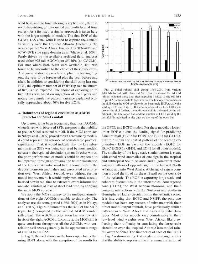
et al. (2009). Figure 2 summarizes the skill of the MOS

(open bar) compared to the skill of AGCM rainfall

(filled bar). The AGCM precipitation has very low skill

in six of the eight AGCMs. In contrast, the MOS skill is

quite consistent throughout all the AGCMs, with cor-

relation skill scores generally in the approximate range

of r 5 0.4 to r 5 0.55.

In Fig. 2, the skill shown in the lower open bar is that

using EOF1 alone, with the exception of the results for

the GFDL and ECPC models. For these models, a lower-

order EOF contains the leading signal for predicting

Sahel rainfall (EOF2 for ECPC and EOF3 for GFDL).

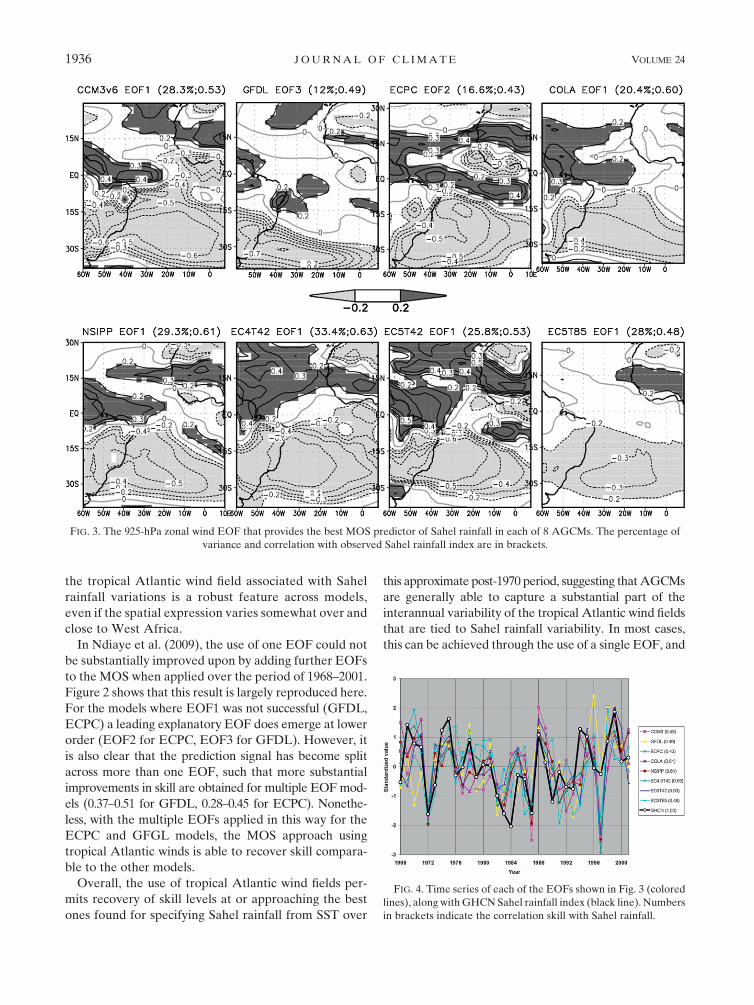
Figure 3 shows the spatial pattern of the leading ex-

planatory EOF in each of the models (EOF2 for

ECPC, EOF3 for GFDL and EOF1 for all other models).

The similarity of the large-scale spatial pattern is clear,

with zonal wind anomalies of one sign in the tropical

and subtropical South Atlantic and a (somewhat more

varying) pattern of opposite sign in the tropical North

Atlantic and into West Africa. A change of sign is com-

mon around the tip of northeast Brazil on the west side

of the Atlantic. The EOF is capturing large-scale and

coherent fluctuations in the intertropical convergence

zone (ITCZ), the West African monsoon, and their

complex interactions with the Northern and Southern

Hemisphere Hadley circulations in the Atlantic sector.

It is interesting that ECPC and NSIPP, the only two

models that have any success of substance with their

direct model-output rainfall, have particularly similar

patterns over West Africa and especially Sahel lati-

tudes. Most other models vary considerably in their

low-level wind weights over West Africa, likely re-

flecting their difficulty in translating the large-scale

circulation over the tropical Atlantic into model rain-

fall over the Sahel. The time series of each of the EOFs

in Fig. 3 is shown in Fig. 4, strongly reinforcing the idea

that the ability to represent the interannual variation of

FIG. 2. Sahel rainfall skill during 1968–2001 from various

AGCMs forced with observed SST. Skill is shown for AGCM

rainfall (shaded bars) and after applying a MOS to the 925-hPa

tropical Atlantic wind field (open bars). The first open bar indicates

the skill when the MOS predictor is the best single EOF, usually the

leading EOF (see Fig. 3). If a combination of up to 5 EOFs im-

proves the skill further, the additional skill is indicated by the ad-

ditional (thin line) open bar, and the number of EOFs yielding the

best skill is indicated by the digit on the top of the open bar.


the tropical Atlantic wind field associated with Sahel

rainfall variations is a robust feature across models,

even if the spatial expression varies somewhat over and

close to West Africa.

In Ndiaye et al. (2009), the use of one EOF could not

be substantially improved upon by adding further EOFs

to the MOS when applied over the period of 1968–2001.

Figure 2 shows that this result is largely reproduced here.

For the models where EOF1 was not successful (GFDL,

ECPC) a leading explanatory EOF does emerge at lower

order (EOF2 for ECPC, EOF3 for GFDL). However, it

is also clear that the prediction signal has become split

across more than one EOF, such that more substantial

improvements in skill are obtained for multiple EOF mod-

els (0.37–0.51 for GFDL, 0.28–0.45 for ECPC). Nonethe-

less, with the multiple EOFs applied in this way for the

ECPC and GFGL models, the MOS approach using

tropical Atlantic winds is able to recover skill compara-

ble to the other models.

Overall, the use of tropical Atlantic wind fields per-

mits recovery of skill levels at or approaching the best

ones found for specifying Sahel rainfall from SST over

this approximate post-1970 period, suggesting that AGCMs

are generally able to capture a substantial part of the

interannual variability of the tropical Atlantic wind fields

that are tied to Sahel rainfall variability. In most cases,

this can be achieved through the use of a single EOF, and

FIG. 3. The 925-hPa zonal wind EOF that provides the best MOS predictor of Sahel rainfall in each of 8 AGCMs. The percentage of

variance and correlation with observed Sahel rainfall index are in brackets.

FIG. 4. Time series of each of the EOFs shown in Fig. 3 (colored

lines), along with GHCN Sahel rainfall index (black line). Numbers

in brackets indicate the correlation skill with Sahel rainfall.


in all cases, a single EOF captures a significant fraction of

the predictable Sahel variance. This encourages use of

this approach in operational seasonal forecast settings

and testing of the approach in the study of coupled model

simulations in the following sections.

4. Predictability from April–May initial conditions

Previous predictability studies of Sahel rainfall have

used prerainfall season SSTs in empirical prediction

models (e.g., Folland et al. 1991; Ward 1998; Thiaw et al.

1999), or AGCMs driven with forecast SST anomalies,

often applying the persistence assumption (Goddard

and Mason 2002). Especially when focusing on the in-

terannual variability of rainfall, a very substantial loss

of skill has generally been found when using SST in-

formation in April and May, as compared to using SST

information in June. This result was isolated using em-

pirical approaches in Ward (1998) and was found in

early AGCM studies (Ward et al. 1993). The result was

also found in Ndiaye et al. (2009) when using the MOS

system applied to the ECHAM4.5 AGCM forced with

persisted SST. The MOS correlation skill was found to

be 0.55 with June SST, 0.33 with May SST, and 0.30 with

April SST.

It is therefore of interest to evaluate the ability of

coupled ocean–atmosphere models to predict Sahel

rainfall, considering both model rainfall and using the

MOS system discussed in the previous section, to see if

skill can be gained at a longer lead time. Furthermore, if

skill is achieved, to assess if the improvements appear

attributable to ocean–atmosphere developments that

were previously not captured in prediction systems.

First, we focus on the results from the CFS, from

which the most comprehensive set of hindcasts is avail-

able to this study, initialized at monthly resolved lead

times and available for the years 1981–2008. The skill of

the model precipitation predictions and the MOS system

predictions are shown in Fig. 5. For now we focus on the

right side of the panel, showing the skill of simulations

that are termed as initialized in April, May, and June.

First, for the CGCM precipitation (shaded bars, Fig. 5),

it is noted that runs initialized in June, May, and April all

display substantial skill. Furthermore, the skill does not

decay but rather is maintained as the lead time increases.

The most likely interpretation of the slight dip in skill

in May, compared to June and April initializations, is

considered due to sampling error rather than a repeat-

able phenomenon.

Applying the MOS system (open bars in Fig. 5) does

not substantially alter the skill levels, but rather, skill is

generally at approximately the same level as achieved

with the model rainfall. However, these MOS results do

demonstrate that use of the low-level wind (mostly EOF1)

is again effective for Sahel prediction, here, in a coupled

forecast system. Furthermore, as diagnosed subsequently

in sections 5 and 6, the skill of the MOS system and the

model rainfall is found to contain somewhat different

aspects of the rainfall variability. The spatial pattern of

the EOF1 of the low-level wind from the CFS runs

initialized in June, May, and April is shown in Fig. 6b,

confirming a similar large-scale spatial pattern compared

to the ones in Fig. 3. Again, consistency is greatest south

of the equator, with more model-specific features emerg-

ing north of the equator, especially over West Africa itself.

The forecast skill shown in Fig. 5 is reproduced when

the Lamb Sahel rainfall index is used as the target pre-

dictand. For example, for the April, May, and June ini-

tializations, the average MOS EOF1 skill using GHCN

is 0.51, whereas using the Lamb index, the average

correlation skill is 0.56. The CFS appears to contain skill

that is comparable to that achieved with observed SST,

and appears to have broken through the problem of

losing skill substantially when forecasts are made using

April information as compared to June information.

The DEMETER CGCMs were all initialized around

1 May, so their Sahel rainfall skill can be compared with

that achieved by systems using April information, and

specifically here, the April initialized runs of the CFS.

The model rainfall and the MOS predicted rainfall

from low-level EOF1 were analyzed in the same way

as reported above for the CFS. For all DEMETER

experiments, 2001 is the last forecast year. MOS pre-

dicted rainfall (Fig. 7a) and CGCMs’ rainfall (Fig. 7b)

are plotted for all available years in 1968–2001 for the

FIG. 5. As in Fig. 2, but for the CFS CGCM (with 850-hPa wind),

showing skill at increasing lead times from June initialization (zero

lead on the JAS Sahel rainfall season) up to December initializa-

tion (6-month lead).


DEMETER models and for the April initialized CFS.

Figure 7 also indicates the years available for each

model and the correlation skill for each model. Most

models (five of seven) show very low levels of skill in

their Sahel rainfall predictions (r , 0.20), with five of

seven showing small increases in skill when the MOS is

applied but with levels of correlation skill still generally

below r 5 0.3. There are two models [the European

Centre for Medium-Range Weather Forecasts (ECMWF),

r 5 0.42; and Max Planck Institute (MPI), r 5 0.49] that

emerge from the set as most promising in their Sahel

rainfall predictions. These skill levels are only compa-

rable or slightly higher than that generally achieved

using persistence approaches. The results do support

the assertion that coupled models are becoming im-

portant contributors to the Sahel rainfall prediction

problem. However, since some predictive information is

known to be present in April SST (e.g., Ward et al. 1993;

Ward 1998), it is difficult to draw the conclusion that the

skill levels represent a clear advance that is attributable

to the CGCM approach. Two aspects motivate a more

detailed analysis of the CFS experiments. First, the CFS

skill levels make a jump that more clearly separates

them from the other models. Second, due to the start

times available for hindcasts, only the skill of models

from initialization around 1 May can be considered for

the DEMETER runs; whereas for the CFS, a much larger

set of hindcasts is available, permitting skill levels to

be established and diagnosed more robustly across vary-

ing lead times.

The level of skill achieved with the CFS is consistent

with the model being able to capture the evolution of the

coupled ocean–atmosphere system through the period

April–June (AMJ) and arrive at a correct representation

of the atmospheric teleconnection response in the tropical

Atlantic wind field and indeed the model output Sahel

precipitation itself. An ability to represent such develop-

ments provides strong support for the CGCM being able

to access sources of skill that are not achievable with

AGCMs, at least when the AGCMs use SST persistence.

The following diagnostic analysis is therefore designed to

assess if the CFS results are rooted in the key coupled

ocean–atmosphere developments for Sahel rainfall.

In Ndiaye et al. (2009), when the persistence approach

led to Sahel forecast failures in the period 1968–2001,

the key SST evolution from April to June was shown to

be associated with developments in the central and eastern

equatorial Pacific. To diagnose the ability of the CFS to

capture such evolution of SST and develop the key tele-

connection structures in the tropical Atlantic, the follow-

ing approach is taken. We first calculate the observed

teleconnection between JAS Nino-3 and the pattern of JAS

SSTs (Fig. 8a) and JAS near-surface (the 1000-hPa level)

winds (Fig. 8b). These represent the teleconnection struc-

tures that need to be in place in the coupled model fore-

casts, especially the linkages from the tropical Pacific to the

tropical Atlantic. First, we address the SST aspects and

then address the wind aspects.

First, to highlight the failure of the persistence ap-

proach for this climate forecast problem, we correlate

FIG. 6. As in Fig. 3, but for the CFS CGCM (with 850-hPa wind), pooling together forecasts for JAS that were

initialized in (a) January, February, and March and (b) April, May, and June.


the JAS Nino-3 index to each SST grid box from April to

June (Fig. 9). While the June map (Fig. 9a) contains

much of the JAS teleconnection structure achieved with

JAS Nino-3 (Fig. 8a), the maps for May and April are

dramatically weaker in the central and eastern tropical

Pacific. The SST correlation over the Nino-3 region is

strong in June (r 5 0.8, Fig. 9a), weakens in May (Fig. 9b)

and drops drastically to about r 5 0.4, and is only signif-

icant over a much smaller area during April (Fig. 9c).

Figure 8a shows the known teleconnection between

El Nino (La Nina) and warmth (cool conditions) in the

tropical North Atlantic (Enfield and Mayer 1997; Lau

and Nath 2001). The panel with April SST (Fig. 9c)

contains a much weaker signal for this tropical North

Atlantic teleconnection, which indicates that the warmth

is usually not already in place in the North Atlantic in

April, in those years that have strong El Nino presence

in JAS (and vice-versa, cool conditions are not in place in

those years when La Nina is present in JAS). Figure 8a

also shows the teleconnection between El Nino (La Nina)

and warmth (cool conditions) in the northwestern Indian

Ocean. Again, Fig. 9c shows that in April, the warmth is

not present in the northwestern Indian Ocean, in those

years when July–September sees the presence of El Nino

(and vice-versa, cool conditions are not in place in those

years when La Nina is present in JAS). So these Indian

and North Atlantic Ocean teleconnection features can be

considered as ones that develop during boreal spring

FIG. 7. Time series of observed Sahel rainfall along with pre-

dicted Sahel rainfall from the seven DEMETER CGCMs (initial-

ized 1 May) and the CFS CGCM (initialized in April). (a) After

applying MOS (same procedure as in Fig. 5) with the best single

EOF and (b) CGCM rainfall. Numbers in brackets indicate the

correlation skill with Sahel rainfall and the forecast years included

in the analysis.

FIG. 8. Observed JAS Nino-3 index correlation 1981–2008 with

(a) observed JAS SST and (b) reanalysis JAS 1000-hPa u and v

wind. A vector is formed using the u correlation (zonal component

of the vector) and the y correlation (meridional component of the

vector). Correlations significant at the 95% level are shaded (for the

wind map, shading is applied if either the u or the v is significant).

FIG. 9. Observed JAS Nino-3 index correlation 1981–2008 with

(a) observed June SST, (b) observed May SST, and (c) observed

April SST. Correlations significant at the 95% level are shaded.


along with Nino-3 development. The tropical North At-

lantic development implies that during an El Nino, the

North Atlantic actually warms. In terms of local SST

forcing on Sahel rainfall, this is consistent with a wetter

Sahel. The warming can therefore be considered a nega-

tive feedback on the large-scale forcing, which generates

atmospheric teleconnection structures from the Pacific to

the Atlantic that favor drier conditions in the Sahel

(Janicot et al. 1996). This was noted in the coupled mode

connecting ENSO to Sahel rainfall in Ward (1998) and

may be one of the reasons why AGCMs have difficulty

with representing the impacts of ENSO directly on the

rainfall because they need to correctly balance these pro-

cesses in the tropical Pacific and Atlantic domains.

A further aspect of Fig. 8a is the negative correlation

with tropical South Atlantic SST. This is not a widely

reported phenomenon in the literature, and when noted,

has been not as easily interpreted in terms of physical

mechanism (Enfield and Mayer 1997). Its presence here

may be amplified through chance sampling in this pe-

riod. Further uncertainty is cast by the fact that the

teleconnection shows as strongest in Fig. 9b, which

suggests tropical South Atlantic SSTs in May are a pre-

cursor of ENSO development into July–September.

Given the difficulties in interpretation, less emphasis is

placed on this SST teleconnection structure, though it

could be worthy of future investigation.

Next, we consider the extent to which CFS forecasts

contain teleconnection structures with the observed JAS

Nino-3. If we were to correlate CFS predicted fields

with the CFS JAS Nino-3, we would obtain the internal

model teleconnection structures. These could be real-

istic but the model might have no predictive capability,

developing ENSOs and associated teleconnection pat-

terns in the wrong years. By using the observed JAS

Nino-3 as the base index for teleconnection maps, the

model must both develop ENSOs in the correct years,

and with the correct teleconnection structure, in order

for the model teleconnection fields to be comparable

with the observed ones in Fig. 8. Therefore, the observed

JAS Nino-3 is correlated with the predicted JAS SST

field that is generated by each of the initialization times.

First, for the tropical Pacific, it is clear that runs initial-

ized in June (Fig. 10a), May (Fig. 10b), and April (Fig. 10c)

all successfully represent the evolution of tropical Pacific

SST to match the observed Nino-3 in JAS and its tele-

connection across the Pacific basin. The performance rep-

resents a substantial improvement upon persistence, as

evidenced by comparing Fig. 9c (April persistence used to

predict JAS SST) with Fig. 10c (April initialized model

prediction of JAS SST).

The CFS also reproduces aspects of the SST de-

velopment in the western Indian Ocean and tropical

Atlantic Oceans. The aspects in the North Atlantic and

western Indian Ocean are actually least clear in the June

initialized results (Fig. 10a), suggesting the longer lead may

allow the CGCM to better develop the teleconnections

between a developing El Nino (La Nina) in the tropical

Pacific and warming (cooling) in the North Atlantic and

the western Indian Ocean (Figs. 10b,c). There is also

a tendency for the negative correlation to be present in

the South Atlantic, such that Figs. 10b and 10c have all

the basic elements in the tropical Atlantic and western

Indian Ocean that are found in the observed teleconnection

structure (Fig. 8a).

These results reveal a good ability to represent the

evolution of SST teleconnections associated with ENSO,

during the buildup to the Sahel rainfall season. A good

ability to represent many key aspects of the correspond-

ing sequence of low-level atmospheric circulation tele-

connections is also seen in Fig. 11. For example, Fig. 11c

shows that CFS runs initialized in April produce JAS

Pacific wind fields that correlate strongly and consistently

with the observed Nino-3 JAS index. The levels of tele-

connection representation are as strong for the April

initializations (Fig. 11c) as they are for the May (Fig. 11b)

and June (Fig. 11a) initializations. The pattern is com-

parable to that achieved between the observed Nino-3

and the observed JAS reanalysis winds (Fig. 8b).

In support of the good skill in predicting Sahel rainfall

(Fig. 5), JAS teleconnection structures in the tropical

FIG. 10. Observed JAS Nino-3 index correlation (1981–2008)

with CFS JAS SST predictions. (a) CFS is initialized in June,

(b) initialized in May, and (c) initialized in April. Correlations

significant at the 95% level are shaded.


Atlantic are also reproduced in the model runs initial-

ized in April, May, and June. In other words, the runs

initialized during boreal spring produce forecast JAS

tropical Atlantic wind fields that correlate with the ob-

served JAS Nino-3 in ways that are largely consistent

with the observed teleconnection structures. For the near-

surface zonal wind, opposite sign correlations are found

in the tropical North and tropical South Atlantic, with the

tip of northeast Brazil being the latitude of the change of

sign in most maps (Fig. 11). The results in Figs. 10 and 11

are interpreted as strong evidence that the results of the

good skill in Sahel prediction are indeed connected to

very large-scale Pacific and Atlantic developments that

are being successfully simulated by the CFS. It lends

considerable support to the hypothesis that the CFS is

able to forecast the key developments from April for

the predictable part of the Sahel rainfall variance that is

related to ENSO.

In summary, the CFS forecasts initialized in April project

tropical Atlantic wind conditions for JAS that correlate

strongly with the observed JAS Sahel rainfall index. A

major part of this is achieved through developments in the

tropical Pacific and tropical Atlantic that are consistent

with the observed climate system teleconnections across

the Pacific–Atlantic sector. This suggests the coupled

model is able to skillfully project forward the coupled

system over this challenging period in the Pacific–Atlantic

sector. Indeed, there is no substantial change in Sahel

rainfall prediction skill when lead time increases from

zero months (June initialization) to two months (April

initialization). This motivates investigation of the addi-

tional CFS runs that are available out to a lead time of six

months (December initialization).

5. Further analysis of the CFS predictability andcomparisons at up to 6-month lead time

The skill of the model precipitation and MOS system

are plotted in Fig. 5 for all runs for which a forecast for

JAS is available from the CFS. The longest lead time

available corresponds to approximately 6 months before

the JAS rainfall season, being initialized in December

and available from 5 January. Figure 5 shows that gen-

erally, for initialization before April, the model pre-

cipitation skill falls quite substantially compared to the

shorter lead-time forecasts. However, for the MOS

on the regional circulation, skill levels are maintained

remarkably stable just using EOF1, even up to the

5-month lead time (January initialization). The leading

EOF spatial pattern is very stable for these initializa-

tions and similar to that found for the shorter lead-time

initializations (cf. Fig. 6a and Fig. 6b). For December

initialization, the skill drops to r 5 0.35 when using just

EOF1 in the MOS system. However, comparable skill

levels are recovered using the leading five EOFS (r 5 0.58).

To confirm that these long-lead forecast skill im-

provements are reflected in large-scale model fields, the

analyses with observed JAS Nino-3 are repeated using

the predicted JAS SST (Fig. 12) and circulation (Fig. 13)

for each of the initialization months. For example, Fig. 12b

shows that even for forecasts initialized in February, pre-

dicted JAS SST in the central and eastern tropical Pacific

correlates over a wide area at over 0.5 with the observed

JAS Nino-3, and since these are correlation values at in-

dividual model gridboxes, the information for the large-

scale atmosphere that is contained in the overall field of

SST in the coupled model may be substantially higher.

In addition, predicted SST in the tropical North At-

lantic and western Indian Ocean continues to correlate

positively with the observed JAS Nino-3, indicating

representation of these teleconnection structures at long

lead time.

The predicted JAS near-surface winds from December

initialization (Fig. 13d) still show a strong and widespread

teleconnection structure with the observed JAS Nino-3

SST. However, the pattern is weakening and especially

so to the north of the equator (cf. Figs. 13d and 13a).

This is true in both the Pacific and in the tropical Atlantic

and may reflect the greater difficulty in recovering the

MOS skill for Sahel rainfall using December initializations.

FIG. 11. As in Fig. 10, but for CFS 1000-hPa wind predictions. A

vector is formed using the u correlation (zonal component of the

vector) and the y correlation (meridional component of the vector).

Shading is applied if either the u or the y correlation is significant at

the 95% level.


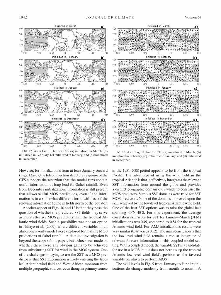
However, for initializations from at least January onward

(Figs. 13a–c), the teleconnection structure response of the

CFS supports the assertion that the model runs contain

useful information at long lead for Sahel rainfall. Even

from December initialization, information is still present

that allows skilful MOS predictions, even if the infor-

mation is in a somewhat different form, with less of the

relevant information found in fields north of the equator.

Another aspect of Figs. 10 and 12 is that they pose the

question of whether the predicted SST fields may serve

as more effective MOS predictors than the tropical At-

lantic wind fields. Such a possibility was not an option

in Ndiaye et al. (2009), where different variables in an

atmosphere-only model were explored for making MOS

predictions of Sahel rainfall. A detailed investigation is

beyond the scope of this paper, but a check was made on

whether there were any obvious gains to be achieved

from substituting SST for wind in the MOS system. One

of the challenges in trying to use the SST as a MOS pre-

dictor is that SST information is likely entering the trop-

ical Atlantic wind field and West African monsoon from

multiple geographic sources, even though a primary source

in the 1981–2008 period appears to be from the tropical

Pacific. The advantage of using the wind field in the

tropical Atlantic is that it effectively integrates the relevant

SST information from around the globe and provides

a distinct geographic domain over which to construct the

MOS predictors. Various SST domains were tried for SST

MOS predictors. None of the domains improved upon the

skill achieved by the low-level tropical Atlantic wind field.

One of the best SST options was to take the global belt

spanning 408N–408S. For this experiment, the average

correlation skill score for SST for January–March (JFM)

initializations was 0.49, compared to 0.54 for the tropical

Atlantic wind field. For AMJ initializations results were

very similar (0.49 versus 0.52). The main conclusion is that

the low-level wind field remains a robust integrator of

relevant forecast information in this coupled model set-

ting. With a coupled model, the variable SST is a candidate

for use in a MOS, but it does not here usurp the tropical

Atlantic low-level wind field’s position as the favored

variable on which to perform MOS.

The skill levels in Fig. 5 from January to June initial-

izations do change modestly from month to month. A

FIG. 12. As in Fig. 10, but for CFS (a) initialized in March, (b)

initialized in February, (c) initialized in January, and (d) initialized

in December.

FIG. 13. As in Fig. 11, but for CFS (a) initialized in March, (b)

initialized in February, (c) initialized in January, and (d) initialized

in December.


substantial part of that is considered to be due to sam-

ple size. To partly confirm that hypothesis, and also to

provide a year-by-year summary of the forecast system,

forecasts have been averaged together across initiali-

zations in January–March and across initializations in

April–June. The model precipitation and MOS results

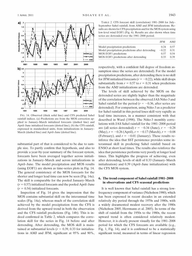
(using EOF1) are shown as time-series plots in Fig. 14.

The general consistency of the MOS forecasts for the

shorter and longer lead time can now be seen (Fig. 14a).

The skill is comparable for the pooled January–March

(r 5 0.57) initialized forecasts and the pooled April–June

(r 5 0.54) initialized forecasts.

Inspection of Fig. 14 gives the impression that the

MOS contains substantial skill on the interannual time

scales (Fig. 14a), whereas much of the correlation skill

achieved by the model precipitation from the CFS is

derived from the upward trend in both the observation

and the CFS rainfall predictions (Fig. 14b). This is in-

deed confirmed in Table 2, which compares the corre-

lation skill for the series in Fig. 14 before and after

detrending. After detrending, the MOS skill is main-

tained at substantial levels (r 5 0.39, 0.33 for initializa-

tions in AMJ and JFM, significant at 95% and 90%,

respectively, with a confident full degree of freedom as-

sumption since the series are detrended). For the model

precipitation predictions, after detrending there is no skill

for JFM initialized forecasts (r 5 20.22), while skill drops

substantially from r 5 0.57 to r 5 0.31 when predictions

from the AMJ initializations are detrended.

The levels of skill achieved by the MOS on the

detrended series are slightly higher than the magnitude

of the correlation between the observed JAS Nino-3 and

Sahel rainfall for the period (r 5 20.36, after series are

detrended). For comparison, using Nino-3 as a predictor

for Sahel rainfall in this period loses skill very rapidly as

lead time increases, in a manner consistent with that

described in Ward (1998). The Nino-3 monthly corre-

lations with JAS Sahel rainfall for the 1981–2008 period

are (all series detrended) r 5 20.34 (June), r 5 20.28

(May), r 5 20.26 (April), r 5 20.17 (March), r 5 20.08

(February), and r 5 20.01 (January). These results re-

inforce the idea that SST persistence provides some in-

terannual skill in predicting Sahel rainfall based on

ENSO at short lead times. The results also reinforce the

idea that persistence performs very poorly at longer lead

times. This highlights the progress of achieving, even

after detrending, levels of skill of 0.33 (January–March

initialization) and 0.39 (April–June initialization) with

the CFS MOS system.

6. The trend component of Sahel rainfall 1981–2008in observations and CFS seasonal predictions

It is well known that Sahel rainfall has a strong low-

frequency component of variance (Nicholson 1980), which

has been expressed in recent decades in an extended

relatively dry period through the 1970s and 1980s, with

a widely documented modest recovery after the 1980s

(Nicholson 2005, Herrmann et al. 2005). In terms of the

shift of rainfall from the 1950s to the 1980s, the recent

upward trend is often considered relatively modest.

However, it is clearly present visually for the 1981–2008

period for which the CFS forecasts are available (e.g.,

Fig. 1, Fig. 14), and it is confirmed to be a statistically

significant trend, measured in terms of linear regression

FIG. 14. Observed (thick solid line) and CFS predicted Sahel

rainfall indices. (a) Predictions are from the MOS correction ap-

plied to January–March initialized forecasts (dashed line) and

April–June initialized forecasts (dotted line), (b) the CFS rainfall,

expressed in standardized units, from initializations in January–

March (dashed line) and April–June (dotted line).

TABLE 2. CFS forecast skill (correlation) 1981–2008 for July–

September Sahel rainfall, from AMJ and JFM initializations. Re-

sults are shown for CFS precipitation and for the MOS system using

low-level wind EOF1 (Fig. 6). Results are also shown when time

series are detrended over the 1981–2008 period.

JFM AMJ

Model precipitation predictions 0.24 0.57

Model precipitation predictions after detrending 20.22 0.31

MOS EOF1 predictions 0.57 0.54

MOS EOF1 predictions after detrending 0.33 0.39


or composite difference. It is therefore considered a real

physical aspect of the climate system, likely to have ex-

pression in large-scale ocean–atmosphere fields, and it is

of interest to consider how the CFS forecast system has

performed in this context. Following analysis and in-

spection of the Sahel rainfall series, the period has been

divided into the relatively dry early set of years (1981–93)

and the more recent wetter years (1994–2008), for the

purpose of constructing composite differences. Table 3

summarizes such differences for the observed Sahel series,

the MOS predictions using EOF1, and the CFS rainfall

predictions, providing quantification and statistical sig-

nificance for the trends in these quantities. In the obser-

vations, the difference is 1.24 standardized units, which is

significant at the 99% level using a t test. This trend is well

captured in the CFS rainfall in both JFM and AMJ ini-

tializations. Both show a strong trend, slightly larger for

the JFM initializations, with a difference of 1.17 and 1.03

standardized units, respectively, with both significant at

the 99% level (Table 3).

The composite analysis also confirms a positive trend

in the MOS predictions using EOF1, though the trend is

weaker, with a difference between the two periods of

0.90 and 0.54 standardized units, respectively, for JFM

and AMJ initializations. The implication is that CFS

wind EOF1 does contain an upward trend but of a mag-

nitude that leads to a somewhat underestimated upward

trend in Sahel rainfall when the MOS prediction system

is applied. Skill statistics are very sensitive to trend (i.e.,

capturing a trend in a set of forecasts can substantially

increase a skill score), and the slightly stronger trend in

the JFM initialized forecasts (Table 3) likely explains

why the JFM MOS predictions do not contain the ex-

pected skill reduction relative to the shorter lead-time

AMJ predictions (Table 2). When the series are de-

trended over 1981–2008, the JFM initialized predictions

do become less skillful than the AMJ initialized pre-

dictions (r 5 0.33 compared to r 5 0.39, Table 2).

Further insight on the trends is gained from composite

difference JAS fields for the low-level wind, precipita-

tion, and SST for observations (Fig. 15; and for the JFM

initialized forecasts, Fig. 16—the composite for AMJ ini-

tialized forecasts has similar structure). In the observed

SST composite difference (Fig. 15a), the first impression

is of a general warming signal, as would be expected

given the known global warming through the period

(Solomon et al. 2007). However, the warming is far from

spatially uniform, and in general, the warming in the

North Atlantic is substantially greater than that in the

South Atlantic. The role of such an arrangement of rel-

ative temperature gradient (including the Indian Ocean

with the South Atlantic) has been previously proposed

in explaining low-frequency Sahel rainfall fluctuations

through the twentieth century (Folland et al. 1991; Rowell

et al. 1995; Hoerling et al. 2006), and an index is used in

many empirical Sahel seasonal prediction systems to

represent this effect (ACMAD 1998). The North Atlantic

part of the interhemispheric SST contrast has been rec-

ognized to project strongly on the Atlantic multidecadal

oscillation (AMO, Enfield et al. 2001), which itself has

been directly associated with low-frequency Sahel rainfall

variations (e.g., Zhang and Delworth 2006; Knight et al.

2006). The implication from Fig. 15a is that a distinct

North Atlantic versus South Atlantic temperature dif-

ference has been evolving through the 1981–2008 period,

with a strong contribution from the AMO (e.g., Ting et al.

2009) and with a sign that would support the increase

in Sahel rainfall precipitation. Consistent changes are

found in the tropical Atlantic wind field (Fig. 15c),

changes that resemble the leading wind EOF discussed

earlier in models, with large-scale fluctuation in the North

and South Atlantic trade wind systems.

Figure 16 reveals the extent to which the CFS fore-

casts contain the above low-frequency climate fluctua-

tions over 1981–2008. First, for the SST composite, the

CFS (Fig. 16a) is generally cooler than observed (Fig. 15a)

in the recent period. However, since the north–south

gradient of SST is hypothesized to be a key factor for

Sahel rainfall, it is important to assess the extent to which

the CFS forecasts are capturing this aspect. The com-

posite maps show that the North Atlantic forecasts for

JAS clearly tend to be warmer than the South Atlantic

TABLE 3. Composite difference of July–September values, 1994–2008 minus 1981–93. Results are for observed and CFS-predicted

precipitation and SST indices. Predictions are initialized in JFM and AMJ. Precipitation results (in standardized units, for the Sahel

region) are shown for observed, CFS predictions, and predictions using the MOS on the low-level wind (Fig. 6). The SST index is AtlN-S

(defined in text), and units are degrees Celsius. Statistical significance is estimated using a t test.

Precipitation SST

CGCM MOS prediction North 2 South Atlantic

Obs CFS JFM CFS AMJ CFS JFM CFS AMJ Obs CFS JFM CFS AMJ

Diff. 1.24 1.17 1.03 0.90 0.54 0.32 0.33 0.29

p value 0.000 0.000 0.000 0.009 0.008 0.000 0.000 0.000


(Fig. 16a). The precipitation (Fig. 16b) over West Africa

and across the tropical Atlantic is also modified in

a manner that is broadly consistent with observations

(Fig. 15b), with enhanced precipitation across the Sahel

and northern side of the ITCZ across the tropical At-

lantic, with a partial compensation in areas to the south

(the partial compensation on the south side is more

pronounced in the model than in observations). Key for

interpreting the MOS rainfall results, the tropical At-

lantic low-level wind field (Fig. 16c) is found to have

a pattern that has resemblance to the EOF1 modes used

in the MOS system, with anomalous easterlies south of

the equator and, more noticeably, anomalous westerlies

north of the equator; although the wind expression is

somewhat weak, especially south of the equator. Thus,

these results are consistent with the EOF1 of the CFS

wind containing a positive trend over the period, but

more weakly than observed, leading to the weaker trends

in the MOS rainfall prediction than observed.

A further aspect of the CFS SST composite (Fig. 16a)

is that it reveals an apparent tendency to predict cool

conditions in the central and eastern equatorial Pacific

during the more recent period. Though it appears the

cooling is more pronounced in the CFS forecasts than it

is in the observations, a tendency to forecast La Nina is

not the dominant feature of the composite trend in the

forecasts. Inspection of the predicted and observed

Nino-3 time series (not shown) shows that there is not

a dramatic bias toward forecasting La Nina develop-

ment and associated cold conditions in the latter period.

Furthermore, if a dominant aspect of the composite

difference for the CFS were a tendency for La Nina in

the recent period, then from the teleconnection struc-

tures of the CFS ENSO in Figs. 10 and 12, warmer

conditions in the South Atlantic and cooler conditions

FIG. 15. Composite difference 1994–2008 minus 1981–93 for

observed JAS fields. (a) SST (8C), (b) rainfall (CMAP dataset,

mm day21), and (c) reanalysis 1000-hPa wind (m s21). For the SST

and rainfall fields, hashing is applied if the difference is significant

at the 95% level using a t test. For the wind field, shading is applied

if either the u or the v difference is significant at the 95% level.

FIG. 16. As in Fig. 15, but for CFS predictions of JAS fields.

Fields shown are the average of predictions initialized in January–

March.


in the North Atlantic would be expected in Fig. 16a.

Therefore, in the Atlantic sector, the trends appear to

represent features that are not a direct response to a

trend in the CFS toward cooler conditions in the eastern

tropical Pacific.

To further investigate the observed and model At-

lantic SST variations over 1981–2008, an index of north

minus south SST over the Atlantic basin (AtlN-S) has

been calculated (Fig. 17). The index is calculated for the

Atlantic domain 308S–608N and is calculated as (608–

108N) minus (108N–308S). The dividing line for the dif-

ference is taken at 108N given the general results in the

literature that show this to be the approximate latitude

at which the zero line of the north–south contrast usu-

ally emerges in July–September teleconnection analyses

with Sahel rainfall (Folland et al. 1986; Rowell et al.

1995) and represents a measure that contrasts SST ap-

proximately to the north and south of the latitude of the

ITCZ at this time of year. As expected from the com-

posite maps (Figs. 15 and 16), the observed and model-

predicted time series of AtlN-S show significant upward

trends (Table 3). The observed JAS index has a positive

correlation with observed Sahel rainfall over this period

(r 5 0.54), consistent with the relationship between such

indices and Sahel rainfall throughout the twentieth cen-

tury (Folland et al. 1986, 1991). The CFS JAS Sahel

rainfall is strongly related to the model’s AtlN-S (r 5 0.55

for AMJ initializations, r 5 0.65 for JFM initializations),

supporting the relationship to be an integral feature of the

model’s regional climate system, as also suggested in the

composite maps (Fig. 16).

Furthermore, it is clear from Fig. 17 that the CFS is

quite effective at containing the AtlN-S information in

its JAS SST predictions, from both JFM initialization

times (r 5 0.64) and AMJ initialization times (r 5 0.78).

Persistence in the observed AtlN-S index is quite high

(r 5 0.53 for JFM to JAS, r 5 0.72 for AMJ to JAS), so

the above skill for the CFS represents a modest improve-

ment on persistence. However, even modest improvement

is noteworthy; it suggests that the CFS skillfully maintains,

over its multimonth forecast, the approximate initialized

AtlN-S anomaly value, and in addition, introduces some

modest skillful developments.

The interpretation is that CFS seasonal forecasts

successfully track many of the observed trends in the

climate of the study region and the Atlantic Ocean.

This is achieved because the CFS contains and skill-

fully projects forward in its seasonal forecasts, varia-

tions of AtlN-S, low-level tropical Atlantic winds, and

Sahel rainfall. The low-level tropical Atlantic winds yield

a modest underestimation of the MOS-predicted Sahel

rainfall. The reason for this underestimation is beyond

the scope of the current paper and requires further in-

vestigation. While adding AtlN-S as a predictor in the

MOS system might be suggested from the above analysis

to yield a better trend in the MOS system, results to this

point do not indicate that such an approach leads to any

major immediate improvement.

7. Conclusions

This paper has addressed two main aspects of Sahel

rainfall prediction. First, results have shown that, when

driven with observed SST, AGCMs usually do contain

information about the observed interannual Sahel rain-

fall variability, through their predictions of the low-level

tropical Atlantic–West Africa wind field. Previous results

have found most AGCMs unable to directly represent

the Sahel’s rainfall variability. Therefore, this new result

is considered to have significant implications about the

utility of AGCMs for prediction of Sahel rainfall in the

context of seasonal time scales, and potentially other time

scales (decadal, climate change), whenever there may be

more confidence in model projections of tropical Atlantic

wind fields as compared to Sahel rainfall. For seasonal

predictions, lead time beyond a month has previously

been a problem even for the best models that represent

Sahel rainfall.

Therefore, the second main aspect presented here has

been the study of coupled models and the potential to

improve the lead time for skillful seasonal forecasts of

Sahel rainfall. Results have identified the potential for

coupled models to break through the lead-time barrier,

with skill superior to that previously reported using em-

pirical or AGCM approaches. Drawing on integrations

with the CFS, skill levels only slightly less than those

achieved by the best approaches using observed SST have

been achieved at lead times of up to six months, utilizing

FIG. 17. Time series of JAS AtlN-S SST. Observed (thick line)

predicted by the CFS from initializations in January–March

(dashed line, r 5 0.64 with observed) and initializations in April–

June (dotted line, r 5 0.78 with observed).


information in the tropical Atlantic–West Africa pre-

dicted wind field.

The CFS skill on the interannual time scale is de-

pendent on applying the MOS approach, and the key

information is captured effectively in the first EOF of

the low-level tropical Atlantic winds. The information

in the tropical Atlantic wind field is confirmed to be part

of large-scale developments in the coupled model in-

volving recognizable teleconnection structures from the

tropical Pacific to the tropical Atlantic in the SST and

low-level wind fields. Documenting these large-scale

teleconnection structures in the model reinforces con-

fidence that the results illustrate the potential of coupled

models to represent the evolution of the climate system

through this period of the annual cycle, and specifically,

to represent key aspects that are relevant for anticipat-

ing Sahel rainfall anomalies.

The period of study with the CFS forecasts (1981–

2008) also contains a significant upward trend in Sahel

rainfall, continuing the low-frequency component of the

region’s climate that has been well documented through

the twentieth century. The CFS forecasts contain the

upward trend, both in model rainfall and the MOS (at

reduced magnitude), and the trend is diagnosed to

a warming in the SST of the North Atlantic (relative to

the South Atlantic), in both observed and model pre-

dicted fields.

While the levels of Sahel rainfall skill achieved through

the CFS at lead times up to 6 months are greater than

found in previous studies, care is required in attributing

and interpreting the skill. AGCMs driven with observed

SSTs have successfully tracked decadal variations in

Sahel rainfall (e.g., Zeng et al. 1999; Giannini et al.

2003; Scaife et al. 2009) and the relevant decadal SSTs

are known to persist from early in the year to boreal

summer (Folland et al. 1991; Ward 1998). Therefore,

over periods when Sahel rainfall exhibits strong de-

cadal fluctuations, it is possible that AGCMs driven

with persisted SSTs may be able to achieve substantial

seasonal forecast skill simply by tracking the decadal

rainfall variations. Such experiments conducted with

the atmospheric component of the CFS over the pe-

riod 1981–2008 would allow clearer attribution of skill

gains to the application of a coupled model approach.

Ideally, assessments would be over a longer period to

allow assessment of model forecast systems over the

1950–present period, taking in a better sample of low-

frequency and high-frequency Sahel rainfall fluctua-

tions. In particular, the AGCM experiments driven with

observed SST reported here (1968–2001) cover a period

that contains a relatively small fraction of variance in the

low frequency, and therefore provides little insight into

the ability of AGCMs to track decadal variations. In

contrast, the period of CFS forecasts (1981–2008) does

contain a substantial low-frequency component (the up-

ward trend), permitting the discussion of the extent to

which the CFS forecasts are both capturing the interannual

variations and tracking the lower frequency trend.

The long lead skill achieved by the CFS after detrend-

ing is scientifically encouraging but requires careful per-

spective in practice. The diagnostic analysis of the coupled

ocean–atmosphere fields strongly suggests that the skill

achieved represents an advance that can be attributed to

the ability to project forward the coupled system by a

CGCM. Previous studies have not found skillful detren-

ded signals in the SST at such long lead times for Sahel

rainfall. However, the level of skill (r 5 0.33 for JFM

initializations) is still modest in practical terms such that

users should consider such a system as providing a mod-

est ability to capture the year-to-year swings in rainfall,

embedded in a more reliable ability to track the lower-

frequency variation.

This study (AGCMs and CGCMs) has focused on

post-1967, the period for which most model simulations

are available, allowing coherent pictures to be drawn

by studying models over comparable years. On the in-

terannual time scale, this period permits a close assess-

ment of skill associated with ENSO but does not allow

a good assessment of the ability to capture the tropical

Atlantic mode of SST variability that was particularly

important for interannual variability in Sahel rainfall

during the wetter regimes of 1950–70 and earlier in the

century (Ward 1998; Janicot et al. 2001). The issue

emerged in the study of Ndiaye et al. (2009), where for

MOS correction focused on AGCM predictions for

1950–70 or including the full period 1950–2000, a second

model wind mode emerged as a MOS predictor that

specified rainfall variability specifically associated with

tropical Atlantic SST. Consideration of this aspect is

beyond the scope of the current paper, but presents itself

as an important question for future study. It is particu-

larly important to address, given the results of Vizy and

Cook (2001), showing that coarse-resolution GCMs can

be expected to have particular difficulty with resolving

the impact of the tropical Atlantic SSTs that give rise

to enhanced (reduced) rainfall in the Sahel with com-

pensating reduced (enhanced) rainfall over the Guinea

Coast region.

A further aspect that is not strongly present in the

1981–2008 period, but has been shown to be a strong

forcing agent on low-frequency Sahel rainfall fluctua-

tions, is low-frequency change in the Indian Ocean SST

(Folland et al. 1986; Giannini et al. 2003). For the pur-

pose of diagnosis here, an index of Atlantic north–south

contrast has been used. It was found that adding In-

dian Ocean SST into the index did not contribute to


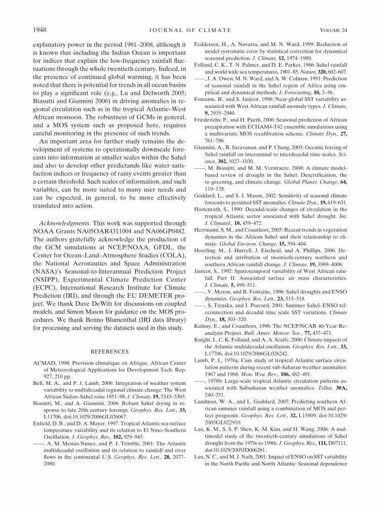
explanatory power in the period 1981–2008, although it

is known that including the Indian Ocean is important

for indices that explain the low-frequency rainfall fluc-

tuations through the whole twentieth century. Indeed, in

the presence of continued global warming, it has been

noted that there is potential for trends in all ocean basins

to play a significant role (e.g., Lu and Delworth 2005;

Biasutti and Giannini 2006) in driving anomalies in re-

gional circulation such as in the tropical Atlantic–West

African monsoon. The robustness of GCMs in general,

and a MOS system such as proposed here, requires

careful monitoring in the presence of such trends.

An important area for further study remains the de-

velopment of systems to operationally downscale fore-

casts into information at smaller scales within the Sahel

and also to develop other predictands like water satis-

faction indices or frequency of rainy events greater than

a certain threshold. Such scales of information, and such

variables, can be more suited to many user needs and

can be expected, in general, to be more effectively

translated into action.

Acknowledgments. This work was supported through

NOAA Grants NA05OAR4311004 and NA06GP0482.

The authors gratefully acknowledge the production of

the GCM simulations at NCEP/NOAA, GFDL, the

Center for Ocean–Land–Atmosphere Studies (COLA),

the National Aeronautics and Space Administration

(NASA)’s Seasonal-to-Interannual Prediction Project

(NSIPP), Experimental Climate Prediction Center

(ECPC), International Research Institute for Climate

Prediction (IRI), and through the EU DEMETER pro-

ject. We thank Dave DeWitt for discussions on coupled

models, and Simon Mason for guidance on the MOS pro-

cedures. We thank Benno Blumenthal (IRI data library)

for processing and serving the datasets used in this study.

REFERENCES

ACMAD, 1998: Prevision climatique en Afrique. African Center

of Meteorological Applications for Development Tech. Rep.

927, 210 pp.

Bell, M. A., and P. J. Lamb, 2006: Integration of weather system

variability to multidecadal regional climate change: The West

African Sudan–Sahel zone 1951–98. J. Climate, 19, 5343–5365.

Biasutti, M., and A. Giannini, 2006: Robust Sahel drying in re-

sponse to late 20th century forcings. Geophys. Res. Lett., 33,

L11706, doi:10.1029/2006GL026067.

Enfield, D. B., and D. A. Mayer, 1997: Tropical Atlantic sea surface

temperature variability and its relation to El Nino–Southern

Oscillation. J. Geophys. Res., 102, 929–945.

——, A. M. Mestas-Nunez, and P. J. Trimble, 2001: The Atlantic

multidecadal oscillation and its relation to rainfall and river

flows in the continental U.S. Geophys. Res. Lett., 28, 2077–

2080.

Feddersen, H., A. Navarra, and M. N. Ward, 1999: Reduction of

model systematic error by statistical correction for dynamical

seasonal prediction. J. Climate, 12, 1974–1989.

Folland, C. K., T. N. Palmer, and D. E. Parker, 1986: Sahel rainfall

and world wide sea temperatures, 1901–85. Nature, 320, 602–607.

——, J. A. Owen, M. N. Ward, and A. W. Colman, 1991: Prediction

of seasonal rainfall in the Sahel region of Africa using em-

pirical and dynamical methods. J. Forecasting, 10, 2–56.

Fontaine, B., and S. Janicot, 1996: Near-global SST variability as-

sociated with West African rainfall anomaly types. J. Climate,

9, 2935–2940.

Friederichs, P., and H. Paeth, 2006: Seasonal prediction of African

precipitation with ECHAM4-T42 ensemble simulations using

a multivariate MOS recalibration scheme. Climate Dyn., 27,

761–786.

Giannini, A., R. Saravanan, and P. Chang, 2003: Oceanic forcing of

Sahel rainfall on interannual to interdecedal time scales. Sci-

ence, 302, 1027–1030.

——, M. Biasutti, and M. M. Verstraete, 2008: A climate model-

based review of drought in the Sahel: Desertification, the

re-greening, and climate change. Global Planet. Change, 64,

119–128.

Goddard, L., and S. J. Mason, 2002: Sensitivity of seasonal climate

forecasts to persisted SST anomalies. Climate Dyn., 19, 619–631.

Hastenrath, S., 1990: Decadal-scale changes of circulation in the

tropical Atlantic sector associated with Sahel drought. Int.

J. Climatol., 10, 459–472.

Herrmann, S. M., and Coauthors, 2005: Recent trends in vegetation

dynamics in the African Sahel and their relationship to cli-

mate. Global Environ. Change, 15, 394–404.

Hoerling, M., J. Hurrell, J. Eischeid, and A. Phillips, 2006: De-

tection and attribution of twentieth-century northern and

southern African rainfall change. J. Climate, 19, 3989–4008.

Janicot, S., 1992: Spatiotemporal variability of West African rain-

fall. Part II: Associated surface air mass characteristics.

J. Climate, 5, 499–511.

——, V. Moron, and B. Fontaine, 1996: Sahel droughts and ENSO

dynamics. Geophys. Res. Lett., 23, 515–518.

——, S. Trzaska, and I. Poccard, 2001: Summer Sahel–ENSO tel-

econnection and decadal time scale SST variations. Climate

Dyn., 18, 303–320.

Kalnay, E., and Coauthors, 1996: The NCEP/NCAR 40-Year Re-

analysis Project. Bull. Amer. Meteor. Soc., 77, 437–471.

Knight, J., C. K. Folland, and A. A. Scaife, 2006: Climate impacts of

the Atlantic multidecadal oscillation. Geophys. Res. Lett., 33,

L17706, doi:10.1029/2006GL026242.

Lamb, P. J., 1978a: Case study of tropical Atlantic surface circu-

lation patterns during recent sub-Saharan weather anomalies:

1967 and 1968. Mon. Wea. Rev., 106, 482–491.

——, 1978b: Large-scale tropical Atlantic circulation patterns as-

sociated with Subsaharan weather anomalies. Tellus, 30A,

240–251.

Landman, W. A., and L. Goddard, 2005: Predicting southern Af-

rican summer rainfall using a combination of MOS and per-

fect prognosis. Geophys. Res. Lett., 32, L15809, doi:10.1029/

2005GL022910.

Lau, K. M., S. S. P. Shen, K.-M. Kim, and H. Wang, 2006: A mul-

timodel study of the twentieth-century simulations of Sahel

drought from the 1970s to 1990s. J. Geophys. Res., 111, D07111,

doi:10.1029/2005JD006281.

Lau, N. C., and M. J. Nath, 2001: Impact of ENSO on SST variability

in the North Pacific and North Atlantic: Seasonal dependence


and role of extratropical air–sea interaction. J. Climate, 14,

2846–2866.

Lu, J., and T. L. Delworth, 2005: Oceanic forcing of the late 20th

century drought. Geophys. Res. Lett., 32, L22706, doi:10.1029/

2005GL023316.

Mo, K. C., and W. M. Thiaw, 2002: Ensemble canonical correlation

prediction of precipitation over the Sahel. Geophys. Res. Lett.,

29, 1570, doi:10.1029/2002GL015075.

Moorthi, S., H.-L. Pan, and P. Caplan, 2001: Changes to the 2001

NCEP operational MRF/AVN global analysis/forecast sys-

tem. NWS Technical Procedures Bulletin, Vol. 484, National

Weather Service, 14 pp.

Ndiaye, O., L. Goddard, and M. N. Ward, 2009: Using regional

wind fields to improve general circulation model forecasts of

July–September Sahel rainfall. Int. J. Climatol., 29, 1262–1275.

Nicholson, S. E., 1980: The nature of rainfall fluctuations in sub-

tropical West Africa. Mon. Wea. Rev., 108, 473–487.

——, 2005: On the question of the ‘‘recovery’’ of the rains in the

West African Sahel. J. Arid Environ., 63, 615–641.

Pacanowski, R. C., and S. M. Griffies, cited 1998: MOM 3.0 manual.

NOAA/GFDL. [Available online at http://www.gfdl.noaa.

gov/_smg/MOM/web/guide_parent/guide_parent.html.]

Palmer, T. N., 1986: Influence of the Atlantic, Pacific and Indian

Oceans on Sahel rainfall. Nature, 322, 251–253.

——, and Coauthors, 2004: Development of a European Multi-

model Ensemble System for Seasonal-to-Interannual Pre-

diction (DEMETER). Bull. Amer. Meteor. Soc., 85, 853–872.

Rowell, D. P., C. K. Folland, K. Maskell, and M. N. Ward, 1995:

Variability of summer rainfall over tropical North Africa

(1906–92): Observations and modelling. Quart. J. Roy. Meteor.

Soc., 121, 669–704.

Saha, S., and Coauthors, 2006: The NCEP climate forecast. J. Cli-

mate, 19, 3483–3517.

Scaife, A. A., and Coauthors, 2009: The CLIVAR C20C project: Se-

lected twentieth-century climate events. Climate Dyn., 33, 603–614.

Semazzi, F. H. M., V. Mehta, and Y. C. Sud, 1988: An investigation

of the relationship between sub-Saharan rainfall and global

sea surface temperatures. Atmos.–Ocean, 26, 118–138.

Smith, T. M., and R. W. Reynolds, 2003: Extended reconstruction

of global sea surface temperatures based on COADS data

(1854–1997). J. Climate, 16, 1495–1510.

Solomon, S., D. Qin, M. Manning, M. Marquis, K. Averyt,

M. M. B. Tignor, H. L. Miller Jr., and Z. Chen, Eds., 2007:

Climate Change 2007: The Physical Science Basis. Cambridge

University Press, 996 pp.

Sud, Y. C., and W. K.-M. Lau, 1996: Comments on ‘‘Variability of

Summer Rainfall over Tropical North Africa (1906–1992):

Observations and Modelling.’’ Quart. J. Roy. Meteor. Soc.,

122, 1001–1006.

Thiaw, W. M., and K. C. Mo, 2005: Impacts of sea surface tem-

perature and soil moisture on the Sahel seasonal rainfall

predictions. J. Climate, 18, 5330–5343.

——, A. G. Barnston, and V. Kumar, 1999: Predictions of African

rainfall on the seasonal timescale. J. Geophys. Res., 104,

31 589–31 597.

Ting, M., Y. Kushnir, R. Seager, and L. Cuihua, 2009: Forced and

internal twentieth-century SST trends in the North Atlantic.

J. Climate, 22, 1469–1481.

Vizy, E. K., and K. H. Cook, 2001: Mechanisms by which Gulf of

Guinea and eastern North Atlantic sea surface temperature

anomalies can influence African rainfall. J. Climate, 14, 795–821.

Ward, M. N., 1998: Diagnosis and short lead time prediction of

summer rainfall in tropical North Africa at interannual and

multidecadal timescale. J. Climate, 11, 3167–3191.

——, C. K. Folland, K. Maskell, A. W. Colman, D. P. Rowell, and

K. B. Lane, 1993: Experimental seasonal forecasting of trop-

ical rainfall at the U.K. Meteorological Office. Prediction

of Interannual Climate Variations, J. Shukla, Ed., Springer–

Verlag, 197–216.

Wolter, K., 1989: Modes of tropical circulation, Southern Oscilla-

tion, and Sahel rainfall anomalies. J. Climate, 2, 149–172.

Wu, R., B. P. Kirtman, and H. van den Dool, 2009: An analysis of

ENSO prediction skill in the CFS retrospective forecasts.

J. Climate, 22, 1801–1818.

Xie, P., and P. A. Arkin, 1997: Global precipitation: A 17-year

monthly analysis based on gauge observations, satellite estimates,

and numerical model outputs. Bull. Amer. Meteor. Soc., 78,

2539–2558.

Zeng, N., J. D. Neelin, K.-M. Lau, and C. J. Tucker, 1999: En-

hancement of interdecadal climate variability in the Sahel by

vegetation interaction. Science, 286, 1537–1540.

Zhang, R., and T. L. Delworth, 2006: Impact of Atlantic multidecadal

osciallations on India/Sahel rainfall and Atlantic hurricanes.

Geophys. Res. Lett., 33, L17712, doi:10.1029/2006GL026267.


Predictability of Seasonal Sahel Rainfall Using GCMs …ousmane/print/pub/Ndiayeetal11_JClim.pdf ·...

Documents

Transcript of Predictability of Seasonal Sahel Rainfall Using GCMs …ousmane/print/pub/Ndiayeetal11_JClim.pdf ·...