1 3

DOI 10.1007/s00382-014-2461-5Clim Dyn

Predictability and prediction skill of the boreal summer intraseasonal oscillation in the Intraseasonal Variability Hindcast Experiment

Sun‑Seon Lee · Bin Wang · Duane E. Waliser · Joseph Mani Neena · June‑Yi Lee

Received: 28 August 2014 / Accepted: 21 December 2014 © The Author(s) 2015. This article is published with open access at Springerlink.com

ratio method and using ensemble-mean approach, we found that the multi-model mean BSISO predictability estimate and prediction skill with strong initial amplitude (about 10 % higher than the mean initial amplitude) are about 45 and 22 days, respectively, which are comparable with the corresponding counterparts for Madden–Julian Oscillation during boreal winter (Neena et al. in J Clim 27:4531–4543, 2014a). The significantly lower BSISO prediction skill compared with its predictability indicates considerable room for improvement of the dynamical BSISO prediction. The estimated predictability limit is independent on its ini-tial amplitude, but the models’ prediction skills for strong initial amplitude is 6 days higher than the corresponding skill with the weak initial condition (about 15 % less than mean initial amplitude), suggesting the importance of using accurate initial conditions. The BSISO predictability and prediction skill are phase and season-dependent, but the degree of dependency varies with the models. It is impor-tant to note that the estimation of prediction skill depends on the methods that generate initial ensembles. Our analy-sis indicates that a better dispersion of ensemble members can considerably improve the ensemble mean prediction skills.

Keywords Boreal summer intraseasnal oscillation · Predictability · Prediction skill · Intraseasonal Variability Hindcast Experiment (ISVHE)

1 Introduction

One of the fundamental features of tropical intraseasonal oscillations (ISOs) is the pronounced seasonal variations in their intensity (Madden 1986), movement (Wang and Rui 1990), and periodicity (Hartmann et al. 1992). The boreal

Abstract Boreal summer intraseasonal oscillation (BSISO) is one of the dominant modes of intraseasonal variability of the tropical climate system, which has fun-damental impacts on regional summer monsoons, tropical storms, and extra-tropical climate variations. Due to its distinctive characteristics, a specific metric for character-izing observed BSISO evolution and assessing numerical models’ simulations has previously been proposed (Lee et al. in Clim Dyn 40:493–509, 2013). However, the current dynamical model’s prediction skill and predictability have not been investigated in a multi-model framework. Using six coupled models in the Intraseasonal Variability Hind-cast Experiment project, the predictability estimates and prediction skill of BSISO are examined. The BSISO pre-dictability is estimated by the forecast lead day when mean forecast error becomes as large as the mean signal under the perfect model assumption. Applying the signal-to-error

S.-S. Lee · B. Wang (*) Department of Meteorology, International Pacific Research Center (IPRC), University of Hawaii, Honolulu, HI, USAe-mail: wangbin@hawaii.edu

B. Wang Earth System Modeling Center/NIAMS, Nanjing University of Information Science and Technology, Nanjing, China

D. E. Waliser · J. M. Neena Joint Institute for Regional Earth System Science and Engineering, University of California, Los Angeles, CA, USA

D. E. Waliser Jet Propulsion Laboratory, California Institute of Technology, Pasadena, CA, USA

J.-Y. Lee Institute of Environmental Studies, Pusan National University, Busan, Korea

S.-S. Lee et al.

1 3

summer ISO (BSISO) exhibits several fundamental char-acteristics that distinguish it from the eastward propagat-ing Madden–Julian Oscillation (MJO) prevailing during boreal winter (Waliser 2006; Goswami 2011): It exhibits prominent northward propagation in the monsoon regions (Yasunari 1979; Krishnamurti and Subrahmanyam 1982; Chen and Murakami 1988) and a significant standing oscil-lation component between the equatorial Indian Ocean and the tropical western North Pacific (Zhu and Wang 1993). It also features a northwest-southeastward tilted rainband (Ferranti et al. 1997; Wang and Xie 1997) and off-equa-torial centers of activity (Kemball-Cook and Wang 2001). The BSISO has complex structures in time and space owing to its interaction with the mean monsoon circulation, the mean state moist static energy distribution (Wang and Xie 1997) and its interaction with warm pool mixed layer (Flatau et al. 1997; Wang and Xie 1998; Wang and Zhang 2002; Fu and Wang 2004; Seo et al. 2007; Krishnamurthy and Shukla 2008; Yun et al. 2008; Lin et al. 2011; Liu and Wang 2013).

While it is known that the BSISO exerts tremendous impacts on the Northern Hemisphere summer monsoons by modulating its onset and active/break cycle (Krishna-murti and Subrahmanyam 1982; Kang et al. 1999; Ding and Wang 2009) and the midlatitude weather and climate through teleconnections (Ding and Wang 2007; Moon et al. 2011, 2013), simulating the BSISO is still a challenge for the current general circulation models (GCMs) (Waliser et al. 2003a; Kim and Kang 2008; Sabeerali et al. 2013). In addition, studies of the BSISO predictability and pre-diction skill have received much less attention than MJO (Waliser 2011). Recently, Fu et al. (2013) investigated the BSISO forecast skill using four state-of-the-art operational and research models. Based on the spatial anomaly correla-tion coefficient, they showed that the intraseasonal forecast skill of the monsoon rainfall and zonal wind is about 1–2 and 3 weeks, respectively, but the target year is confined to 2008 summer only. For the BSISO predictability, it is found that the mean predictability of the monsoon ISO-related rainfall over the Asian–western Pacific region (10°S–30°N, 60°–160°E) reaches about 24 days in the coupled model and this is 1 week higher than in the atmosphere-only model (Fu et al. 2007).

To evaluate the predictability and prediction skill of the intraseasonal variability in a multi-model framework, the Intraseasonal Variability Hindcast Experiment (ISVHE) was launched in 2009. Using this ISVHE hindcast data, Neena et al. (2014a) examined the predictability of MJO in eight coupled climate models based on the real-time multivariate MJO (RMM) index, which is the most popu-lar MJO index (Wheeler and Hendon 2004). They found that, in most models, the MJO predictability estimated by the signal-to-noise ratio using the single-member

and ensemble-mean hindcasts was around 20–30 and 35–45 days, respectively. Furthermore, the prediction skill and predictability of the eastern Pacific ISV during boreal summer is also evaluated using the ISVHE data (Neena et al. 2014b). However, the current models’ prediction skills and predictability of BSISO in multi-model frame-work have not been examined. Therefore, the main purpose of the present study is to estimate the predictability and evaluate the current prediction capability of BSISO using the ISVHE hindcast data. This is the first study to assess the BSISO predictability and prediction skill in a multi-model framework. Based on this study, we can establish a foothold to develop the optimal strategies for multi-model ensemble (MME) BSISO prediction system.

The description of the hindcast data is presented in Sect. 2. Section 3 describes the procedure for calculating BSISO index in both observation and hindcast. Methods for estimating predictability and prediction skill are also given. The predictability and prediction skill in the ISVHE hind-cast are compared in Sect. 4, focusing on their sensitivity on the initial amplitude, initial phase, and initial month. In Sect. 5, the relationship between dispersion of the ensem-ble members and prediction skill improvement is analyzed. Summary and discussion follow in Sect. 6.

2 ISVHE hindcast data

The ISVHE (https://yotc.ucar.edu/modeling/isvhe-intra-seasonal-variability-hindcast-experiment) is a coordinated multi-institutional experiment supported by Asian Pacific Climate Center (APCC), National Oceanic and Atmos-pheric Administration (NOAA) Climate Test Bed (CTB), Climate Variability and Predictability (CLIVAR)/Asian-Australian Monsoon Panel (AAMP), Year of Tropical Con-vection (YOTC; Moncrieff et al. 2012; Waliser et al. 2012) and its MJO Task Force, and Asian Monsoon Years (AMY). The aim of ISVHE is to better understand the physical basis for ISV prediction and determine the predictability of ISV in a multi-model framework. The ISVHE includes two sets of experiments, a long-term free run (AMIP-type run) and the hindcast experiment. This project is the first attempt to produce long-term hindcast datasets from multiple GCMs.

There is no requirement for a standard initialization pro-cedure for atmosphere, land, and ocean. Most participating climate models fulfill the minimum specifications includ-ing (a) predictions initiated every 10th day on 1st, 11st, and 21st of each calendar month throughout the entire 20-year period; (b) a minimum integration length of 45 days; (c) at least 5 ensemble members for each forecast. In the pre-sent study, we have analyzed the hindcast data for summer (from May to October) made by six coupled models and details of hindcast data is presented in Table 1.

Predictability and prediction skill of the BSISO

1 3

3 Methodology

3.1 Calculation of BSISO index in observation and hindcast

To better capture the observed northward propagating ISO over the Asian summer monsoon (ASM) region, Lee et al. (2013) proposed two BSISO indices based on multivariate empirical orthogonal function (MV-EOF) analysis (Wang 1992) of daily anomalies of outgoing longwave radiation (OLR) and 850-hPa zonal wind (U850) over [10°S–40°N, 40°–160°E]. The BSISO1, consisting of EOF1 and EOF2 modes, represents the canonical northward propagating ISO during the entire warm season (from May to October) with quasi-oscillating periods of 30–60 days. The BSISO2, consisting of EOF3 and EOF4 modes, captures the north-ward/northwestward propagating variability with periods of 10–30 days during primarily the pre-monsoon and mon-soon-onset season.

In the present study, we have followed the same pro-cedure as Lee et al. (2013) to obtain the observed BSISO indices and we focused on only BSISO1 (PC1 and PC2) (hereafter ‘BSISO index’). For the observed BSISO index, the OLR is obtained from NOAA polar-orbiting series of satellites with 2.5° horizontal resolution (Lieb-mann and Smith 1996) and U850 is from the National Centers for Environmental Prediction (NCEP)/Depart-ment of Energy (DOE) Reanalysis II (Kanamitsu et al. Kanamitsu et al. 2002). The OLR and U850 anomalies were obtained by removing the slow annual cycle (the annual mean and the first three harmonics of climatologi-cal annual variation) and the interannual variability (run-ning mean of the preceding 120 days) (Lee et al. 2013). The climatology and normalization factor were com-puted for the period from May 1st to October 31st during 30 years (1981–2010).

For the hindcast BSISO index in individual mod-els, the model climatology which is a function of initial condition (starting date of hindcast) and lead day (Zhu et al. 2014) was first removed from the OLR and U850 hindcast fields. The effect of interannual variability was further removed by subtracting the running mean of the last 120 days. In this process, we used observed anom-alies before the start day of hindcast to make enough data for the running mean (Lin et al. 2008; Neena et al. 2014a). Two hindcast anomaly fields were normal-ized by area-averaged temporal standard deviation over the ASM region obtained from the observed OLR and U850. Finally, the hindcast BSISO index was obtained by projecting the two combined anomaly fields onto the observed BSISO EOF modes. The observed and hindcast BSISO indices were normalized by standard deviation of observed BSISO index.Ta

ble

1 D

etai

ls o

f hi

ndca

st d

ata

of th

e si

x m

odel

s

Mod

elH

indc

ast

peri

odN

umbe

r of

en

sem

ble

mem

bers

Initi

aliz

atio

nsE

nsem

ble

gene

ratio

n m

etho

dR

efer

ence

s

AB

OM

1

PO

AM

A 1

.5 (

AC

OM

2 +

BA

M3)

1980

–200

610

The

1st

day

of

ever

y m

onth

6-h

lagg

ed a

tmos

pher

ic in

itial

con

ditio

nsC

olm

an e

t al.

(200

5)

AB

OM

2

PO

AM

A 2

.4 (

AC

OM

2 +

BA

M3)

1989

–200

810

The

1st

day

and

11t

h

of e

very

mon

thPe

rtur

batio

ns u

sing

cou

pled

br

ed v

ecto

rsC

ottr

ill e

t al.

(201

3)

EC

MW

F

EC

MW

F (I

FS +

HO

PE)

1989

–200

85

The

1st

day

of

ever

y m

onth

Pert

urba

tions

usi

ng c

oupl

ed

bred

vec

tors

Alv

es e

t al.

(200

4),

Via

lard

et a

l. (2

005)

JMA

C

JM

A C

GC

M19

89–2

008

5E

very

15t

h da

yPe

rtur

batio

ns u

sing

sin

gula

r ve

ctor

sIs

hika

wa

et a

l. (2

005)

, JM

A (

2007

)

CM

CC

CM

CC

(E

CH

AM

5 +

OPA

8.2)

1989

–200

75

Eve

ry 1

0th

day

1-da

y la

gged

initi

al c

ondi

tions

Ale

ssan

dri e

t al.

(201

5)

CFS

2

NC

EP/

CPC

CFS

v2

1999

–201

04

The

1st

, 11t

h an

d 21

st

day

of e

very

mon

th6-

h la

gged

initi

al c

ondi

tions

Saha

et a

l. (2

014)

S.-S. Lee et al.

1 3

3.2 Estimation of predictability and prediction skill

The hindcast can be evaluated from the probabilistic and/or deterministic perspective. A probabilistic skill estimates the probability of occurrence of a chosen event and one of the widely used methods is Brier skill score. The deterministic skill measures the actual value of the quantity of interest and includes the anomaly correlation coefficients in time/space and mean square error. In the present study, to esti-mate the predictability and prediction skill, we applied the signal-to-noise (signal-to-error) ratio method that has been used in several other studies (Waliser et al. 2003a, b; Liess et al. 2005; Fu et al. 2007, 2008; Pegion and Kirtman 2008; Neena et al. 2014a, b). Specifically the ‘single-member method’ and ‘ensemble-mean method’ (Neena et al. 2014a) were applied, and thus we can compare the predictability and prediction skill of BSISO with those of MJO in the same metric.

Under the perfect model assumption, it is considered that the forecast is composed of a ‘control’ and a ‘per-turbed’ initial conditions. For the single-member method, the forecast error at the forecast lead day ‘j’ in a particular initial condition time ‘i’ (E2

ij) is defined as the difference of BSISO index (PC1 and PC2) between the control and per-turbation (Eq. 1).

In the above equation, ctl means one of the ensemble members designated as a control and ptb indicates any other ensemble members other than ctl. This procedure is repeated for all ensemble members that are designated as a control. The mean forecast error for a given forecast lead day is computed over all different pairs (P) of [ctl and ptb] and over N different initial conditions (Eq. 2).

The signal at the forecast lead day ‘j’ in a particular ini-tial condition time ‘i’ (S2

ij) is defined by the mean amplitude of the BSISO index designated as a control within a sliding window (2L + 1), which covers one complete BSISO cycle (Eq. 3). L is set to 25 days in the present study (i.e. 51 day average).

In Neena et al. (2014a), the observed values prior to hindcast initiation day were used for computing the signal

(1)

E2ij = (BSISOPC1ij,ctl − BSISOPC1ij,ptb)

2

+ (BSISOPC2ij,ctl − BSISOPC2ij,ptb)2

(2)E2j =

1

NP

N∑

i=1

P∑

[ctl,ptb]

E2ij

(3)S2ij =

1

2L + 1

L∑

t=−L

(BSISOPC12ij+t + BSISOPC2

2ij+t)

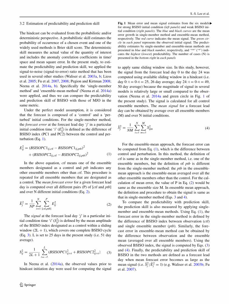
to apply same sliding window size. In this study, however, the signal from the forecast lead day 0 to the day 24 was computed using available sliding window in a hindcast (i.e. day 0: t = 0–t = 25, 26 day average; day 24: t = 0–t = 49, 50 day average) because the magnitude of signal in several models is relatively large or small compared to the obser-vation (Neena et al. 2014a and green circle in Fig. 1 of the present study). The signal is calculated for all control ensemble members. The mean signal for a forecast lead day can be obtained by average over all ensemble members (M) and over N initial conditions.

For the ensemble-mean approach, the forecast error can be computed from Eq. (1), which is the difference between control and perturbation. In this method, the definition of ctl is same as in the single-member method, i.e. one of the ensemble members, but the definition of ptb is different from the single-member method: the ptb in the ensemble-mean approach is the ensemble-mean averaged over all the other ensemble members other than the control. For the cal-culation of mean error, the value of P in Eq. (2) would be same as the ensemble size M. In ensemble mean approach, the definition and procedure to obtain the signal is same as that in single-member method (Eqs. 3 and 4).

To compare the predictability with prediction skill, the prediction skill is also measured by applying single-member and ensemble-mean methods. Using Eq. (1), the forecast error in the single-member method is defined by the difference of BSISO index between observation (ctl) and single ensemble member (ptb). Similarly, the fore-cast error in ensemble-mean method can be obtained by the difference between observation and the ensemble mean (averaged over all ensemble members). Using the observed BSISO index, the signal is computed by Eqs. (3) and (4). Finally, the predictability and prediction skill of BSISO in the two methods are defined as a forecast lead day when mean forecast error becomes as large as the mean signal (i.e. S2

j /E2j = 1) (e.g. Waliser et al. 2003b; Fu

et al. 2007).

(4)S2j =

1

NM

N∑

i=1

M∑

m=1

S2ijm

Fig. 1 Mean error and mean signal estimates from the six models for strong BSISO initial condition (left panels) and weak BSISO ini-tial condition (right panels). The blue and black curves are the mean error growth in single-member method and ensemble-mean method, respectively. The red curve indicates the mean signal. The green cir-cle in each panel represents the observed initial signal. The predict-ability estimates by single-member and ensemble-mean methods are presented in blue and black number, respectively, and ‘**’ (‘*’) indi-cates the highest (lowest) predictability. The number of cases (N) is presented in the bottom-right in each panels

▸

Predictability and prediction skill of the BSISO

1 3

S.-S. Lee et al.

1 3

4 Predictability and prediction skill of BSISO

4.1 Dependency on initial amplitude

First, we examined the dependence of BSISO predictabil-ity and prediction skill on the initial amplitude by compari-son of two groups that have strong and weak BSISO initial amplitudes. The mean amplitude of observed BSISO index [i.e. (PC12 + PC22)1/2] at forecast lead day 0 is about 1.18. Therefore, we defined the strong BSISO initial condition as the amplitude of observed BSISO index at forecast lead day 0 is greater than 1.3 [i.e. (PC12 + PC22)1/2 > 1.3]. This indicates that when we calculate the mean signal and mean error in individual models, hindcasts were included only if the observed BSISO amplitude at forecast lead day 0 was greater than 1.3. Similarly, weak BSISO initial condition is defined as the amplitude of observed BSISO index at fore-cast lead day 0 is less than 1.0 [i.e. (PC12 + PC22)1/2 < 1.0]. Under these criteria, in all six models, the number of strong initial condition case is comparable to that of weak initial condition. Unlike Neena et al. (2014a), we don’t consider the initial phase for this comparison.

Figure 1 shows the mean error growth estimated by single-member and ensemble-mean methods as well as the corresponding mean signal in strong and weak BSISO ini-tial conditions, respectively. In addition, following Neena et al. (2014a), the observed signal at day 0 is presented by green circle in each panel of Fig. 1 to compare it with the hindcast initial signal. The initial signals of ABOM1 and

ABOM2 are nearly the same as observation in both the strong and weak BSISO initial conditions, while JMAC and CMCC present very weak signal compared to the observed value.

As mentioned before, the predictability can be estimated from the forecast lead days when the error is as large as the signal. In all models, the predictability estimated by the ensemble-mean approach is much higher than that by the single-member approach because of the slower error growth in the ensemble-mean method. For strong BSISO initial condition, the resultant multi-model mean predict-ability estimated by the single-member method is about 18 days (ranging from 12 to 23 days) while that estimated by the ensemble-mean method is about 45 days (ranging from 38 to 55 days). In the single-member method, CFS2 shows the highest predictability (23 days) while ABOM2 shows the lowest predictability (12 days). This value is lower compared to MJO predictability, showing the range from 18 to 28 in strong MJO initial condition (with con-sideration of phase) (Neena et al. 2014a). In the ensemble-mean method, the predictability yields a large range from 38 days in ECMWF to 55 days in ABOM1 and this is com-parable with MJO.

For the weak BSISO initial condition, the multi-model mean predictability by single-member and ensemble-mean methods is about 17 days (ranging from 10 to 22 days) and 44 days (ranging from 27 to 55 days), respectively. (In CFS2, the predictability was not estimated by ensemble-mean method for its integration days.) These values are

Fig. 2 The predictability (±5 days range) and prediction skill of BSISO in a strong BSISO initial condition and b weak BSISO initial condition

Predictability and prediction skill of the BSISO

1 3

slightly lower than those in strong BSISO initial amplitude, but the difference is not statistically significant. This result indicates that the BSISO predictability is not dependent on the initial amplitude, which is in contrast to the boreal winter MJO predictability that tends to be dependent on the MJO amplitude in the initial condition (Waliser et al. 2003b; Neena et al. 2014a).

The current prediction skill for BSISO in strong and weak initial conditions is compared with predictabil-ity (Fig. 2). In both initial conditions, the prediction skill obtained by the ensemble-mean method is evidently bet-ter than that of the single-member method. Furthermore, different from the predictability, the prediction skill with strong initial amplitude is better than that with weak initial amplitude for both methods in most models. In the ensem-ble-mean approach, the multi-model mean prediction skill under the strong BSISO initial condition is about 22 days, while corresponding skill with the weak BSISO initial con-dition is about 16 days. This result suggests the dependency of prediction skill on the initial amplitude. For the MJO prediction skill, coupled models show ensemble-mean pre-diction skill ranging from 7 (CFS1) to 28 days (ECMWF) in strong MJO initial condition (Neena et al. 2014a). Lin et al. (2008), who studied MJO predictability using two atmospheric models, showed that forecast skill initialized with large MJO amplitude is better than that with a weak MJO initial signal.

For both the strong and weak initial amplitudes, the comparison between the prediction skill and predictability suggests that the current single-member and ensemble-mean prediction skills can be further improved by about 5–7 and 23–28 days, respectively. In addition, the predic-tion skill gap between single-member method and ensem-ble-mean method is larger in the strong BSISO initial conditions.

4.2 Dependency on initial phase

The dependency of ISO predictability and prediction skill on various phases is one of the controversial issues because those are dependent on the data and method (e.g. Waliser et al. 2003b; Seo et al. 2005; Lin et al. 2008; Kang and Kim 2010; Ding et al. 2011; Fu et al. 2011). Neena et al. (2014a) found that the MJO predictability initiated from MJO phase 2, 3 (Indian Ocean) or 6, 7 (Western Pacific) is slightly higher than other phases in several models, but systematic phase dependency was not observed in all models. In this subsection we explore the initial phase dependency of the BSISO prediction/predictability in ISVHE hindcast data. Lee et al. (2013) divided the BSISO life cycle into eight phases based on the sign and magnitude of PC1 and PC2. The same method for phase definition was applied in the present study.

Figure 3 presents the predictability and prediction skill according to different BSISO initial phases by the ensem-ble-mean approach. For this analysis, the initial amplitude was not considered in order to secure enough samples. It is found that there is no systematic predictability depend-ency on the initial phase, although in some models the pre-dictability initiated from the specific phase is significant at the 95 % confidence level based on a Student’s t test. The predictability difference between different initial phases is very large in ABOM1 (range from 27 to 54 days) and ABOM2 (range from 25 to 41 days) while that is small in JMAC (range from 33 to 37 days) and CFS2 (range from 39 to 43 days). Similar to the predictability, the prediction skill is not systematically dependent on the initial phase. The ECMWF, JMAC, CMCC and CFS show the highest prediction skill with the initial phase 1 and 8 (Equatorial Indian Ocean and western North Pacific). But this highest skill is not significant compared with other phases in all

Fig. 3 The predictability and prediction skill initiated from different initial phases. The error bars of predictability represent the 95 % confidence interval. The table at the bottom-right gives the number of cases (N)

S.-S. Lee et al.

1 3

four models (not shown). The prediction skill with the ini-tial phase 6 and 7 (Bay of Bengal and South China Sea) is over 20 days in the ECMWF and JMAC whereas corre-sponding prediction skills in other four models exhibit the lowest.

Furthermore, the sensitivity of the predictability to both initial phase and initial amplitude were compared (Fig. 4), similar to what have been done in the previous subsection. Note that, in this comparison, the sample size in several cases is relatively small since we considered both initial amplitude and initial phase. For strong BSISO initial condi-tion, four models (ABOM2, ECMWF, JMAC, CFS2) out of the six models show the lowest predictability when it is initiated from BSISO phase 2 and 3 (Indian Ocean and East Asia) but that is not significant (Fig. 4a). With weak BSISO initial amplitude, it is also found that there is no systematic dependence of predictability on the initial phase (Fig. 4b) and the predictability varies considerably with models.

4.3 Dependency on initial month

Seasonal prediction skills show season-dependence, i.e. the prediction starting from a specific month may achieve a higher forecasting skill than starting from other months

(Lee et al. 2011). Since the BSISO involves strong modu-lation of convectively coupled waves by mean flow and the mean circulation has large seasonal change (Kemball-Cook and Wang 2001), it is meaningful to examine whether the prediction skill and predictability vary with seasonal march. Therefore, in this subsection, the dependency of BSISO predictability and prediction skill on the initial month is investigated. For fair comparison, we selected just three models that are all initialized from the 1st day of every month. The CFS2 was not included because its hind-cast period is relatively short (1999–2010, 12 years) com-pared to other three models (19–20 years).

Figure 5 exhibits predictability and prediction skill as a function of initial month estimated by the ensemble-mean method. In each model, the estimated predictability and prediction skill vary with initiation month but systematic season-dependency is not found across all three models. Thus, the dependency of the predictability and predic-tion skill on initial month is highly model dependent. For instance, in ABOM the highest predictability initiated from May 1st is significant at the 95 % confidence level based on a Student’s t test compared to July and August initial con-ditions. In CMCC, however, the highest predictability with May 1st initial condition is significant compared with only

Fig. 4 The predictability initiated from different initial phases with a strong BSISO initial condition and b weak BSISO initial condition. The error bars of predictability represent the 95 % confidence interval. The tables at the bottom give the number of cases (N)

Predictability and prediction skill of the BSISO

1 3

October initial condition. ECMWF shows the significant lowest predictability with May 1st initial condition and pre-dictability varies greatly with the initial condition.

For the prediction skill, ECMWF has better prediction skill with a range from 16 days in July 1st initial condi-tion to 29 days in August and September 1st initial condi-tions compared to other two models. In addition, the high-est prediction skill is significant compared with the lowest prediction skill. The ABOM2 and CMCC, however, exhibit the best prediction skill with October and June 1st initial condition, respectively.

5 Relation between dispersion of initial ensembles and prediction skill improvement

Different ensemble generation methods were applied in all six models used in the present study (Table 1) and the methods for generating initial ensembles are related to the dispersion of ensemble members. To assess the merit of the different existing ensemble techniques, Buizza et al. (2005) compared the operational ensemble forecasts generated at three operational numerical weather prediction centers (ECMWF, NCEP, Meteorological Service of Canada). They found that the performance of ensemble prediction systems strongly depends on the quality of the data assimilation

system used to create the initial condition. In addition, the spread of ensemble forecasts in three centers is insufficient to simulate all sources of forecast uncertainty.

In this subsection, we evaluated the reliability of the six ensemble prediction systems in terms of the relation-ship between the dispersion of ensemble members and the prediction skill improvement. Here the prediction skill improvement indicates the difference of prediction skills measured by the single-member approach and ensemble-mean approach. A well dispersed ensemble is often referred to as a “well calibrated” ensemble. In statistically consist-ent ensembles, the standard deviation of ensembles (i.e. ensemble spread) should match the root-mean square error (RMSE) of the ensemble-mean (e.g. Talagrand et al. 1999; Buizza et al. 2005; Eckel and Mass 2005; Weisheimer et al. 2009, 2011). Therefore, the dispersion of ensembles can be measured by the difference between ensemble spread and the RMSE of the ensemble-mean. Following Neena et al. (2014a), the ensemble spread for a given forecast lead day and initial condition is defined as the combined standard deviations of PC1 and PC2 (BSISO index) in the ensem-ble member hindcast. The respective ensemble-mean value at the corresponding forecast lead day and initial condition was used. The RMSE of ensemble-mean was obtained by the RMSE between the observed and ensemble-mean hind-cast BSISO index (Lin et al. 2008). The ensemble spread

Fig. 5 The a predictability and b prediction skill initiated from different initial months. The error bars in a, b the 95 % confidence interval. The table at the bottom gives the number of cases (N)

S.-S. Lee et al.

1 3

and ensemble-mean RMSE were averaged over all summer initial conditions (from May to October of the entire hind-cast periods).

Figure 6a shows the ensemble spread (solid lines) and ensemble-mean RMSE (dashed lines) as a function of fore-cast lead days. In all six models, the ensemble spread is always smaller than the ensemble-mean RMSE, indicating that initial ensembles generated in six coupled models are less dispersive, and thus do not capture all possible sources of error from internal dynamics (Vialard et al. 2005). This result is consistent with Neena et al. (2014a) who showed that the all models for MJO are under-dispersive ensemble prediction system. If the ensemble spread is too small to represent the full amount of uncertainty in the prediction, it indicates that the ensembles are overconfident. Using the ensemble spread and ensemble-mean RMSE, the degree of dispersion is measured by the mean difference between ensemble spread and ensemble-mean RMSE (i.e. solid line

minus dashed line) averaged for the first 25 days in an indi-vidual model (Fig. 6b). This difference is called here the “quality of dispersion”. Since the RMSE of the ensemble-mean would equal the ensemble spread in the statistical consistency, a smaller value of dispersion quality indi-cates a better dispersed ensemble prediction system. In the ABOM2 and ECMWF, the two corresponding (solid and dashed) lines are close to each other (Fig. 6a) and therefore the difference between the two corresponding lines is small (Fig. 6b). This implies that these two models provide rela-tively well-dispersed ensembles. In JMAC, however, the ensemble spread is the lowest (Fig. 6a) and the quality of dispersion shows the largest negative value (Fig. 6b), indi-cating each individual ensemble in this system is substan-tially under-dispersive.

Furthermore, the relationship between the quality of dis-persion and the skill improvement was examined (Fig. 6d). As aforementioned, the skill improvement is defined as the

Fig. 6 a Ensemble spread (solid lines) and ensemble-mean RMSE (dashed lines). b The 25 day forecast lead average of the differ-ence between ensemble spread and ensemble-mean RMSE for each model. c Prediction skill by single-member method (sky blue) and ensemble-mean method (orange) with all summer initial conditions.

d The 25 day forecast lead average of the difference between ensem-ble spread and ensemble-mean RMSE for each model [values in (b)] (x-axis) and skill improvement [ensemble-mean prediction skill minus single-member prediction skill in (c)] (y-axis)

Predictability and prediction skill of the BSISO

1 3

difference between the ensemble-mean prediction skill and single-member prediction skill obtained from all summer initial conditions (Fig. 6c). The ECMWF and ABOM2, which are better dispersed ensemble prediction systems, show the significant improvement of prediction skill (about two times higher ensemble-mean prediction skill than the single-member prediction). Consequently, results obtained from Fig. 6 suggest that ensemble-mean prediction skill could be significantly improved by the well-dispersed ini-tial ensemble forecasts.

6 Summary and discussion

6.1 Summary

We examined the BSISO prediction skill and estimated its predictability in order to better understand the way to nar-row down the gap between the present day prediction capa-bilities and the predictability limit. For the analysis of pre-dictability and prediction skill, we utilized the BSISO index proposed by Lee et al. (2013), which is based on the MV-EOF analysis of daily anomalies of OLR and U850 in the region (10°S–40°N, 40°–160°E). Using the daily hindcast data from six coupled climate models that participated in ISVHE project, the hindcast BSISO index was obtained by projecting the combined OLR and U850 anomalous fields onto observed BSISO EOF modes. Methods used to meas-ure the predictability and prediction skill of BSISO include the single-member and ensemble-mean approaches based on the perfect model assumption, and we mainly focused on the estimations by the ensemble-mean approach.

The dependences of the predictability and prediction skill estimates on the initial amplitude, initial phase, and initial month were assessed. We summarize the results of BSISO predictability and prediction skill by comparing it with MJO results documented by Neena et al. (2014a). The BSISO pre-dictability is not dependent on the initial amplitude (Figs. 1, 2), and this feature is different from MJO predictability which shows the initial amplitude dependency. Multi-model mean predictability with strong BSISO initial amplitude is esti-mated about 45 days by ensemble-mean method, and this is only 1 day higher than that in weak BSISO initial ampli-tude. For MJO, 35–45 days ensemble-mean predictability is obtained from strong MJO initial amplitude in the eight mod-els. The estimated predictability initiated from weak MJO is 5–10 days lower compared to that initiated from strong MJO. In terms of the initial phase dependency, for MJO predictabil-ity, several models among eight climate models tend to show slightly higher predictability initiated from MJO phases 2, 3 (Indian Ocean) or 6, 7 (Western Pacific) (Neena et al. 2014a). For the BSISO predictability, there is no systematic depend-ency on the initial phase and the predictability from different

initial phases varies considerably with models (Figs. 3, 4). The BSISO predictability tends to be season-dependent, but the concrete season-dependence varies with models (Fig. 5).

Different from BSISO predictability, the BSISO predic-tion skill is better for the events with large initial amplitude, indicating the importance of using accurate initial conditions (Fig. 2). In strong initial amplitude, prediction skill of BSISO measured by ensemble-mean approach is about 22 days and this value is comparable with that of MJO. The correspond-ing prediction skill with the weak BSISO initial condition is about 16 days. The gap of actual prediction skill and predict-ability estimated by ensemble-mean approach in six climate models is about 3–4 weeks and this suggests room for con-siderable improvement of the BSISO prediction. It is noted that initial phase dependence and initial month dependence of prediction skill are highly model dependent.

Finally, it is found that an improved dispersion of initial ensembles in the ensemble prediction system can lead to significant improvement of ensemble-mean prediction skills (Fig. 6). The ensemble-mean prediction skill is considerably improved in ECMWF and ABOM2, which exhibit relatively better quality of ensemble dispersion. This confirms that the conclusions derived from the MJO study (Neena et al. 2014a) also apply to the BSISO. Since the ensemble genera-tion method is certainly related to the improvement of fore-cast performance for intraseasonal variability (Hudson et al. 2013), the development of ensemble generation strategy is essential for better prediction skill of ISV.

6.2 Discussion

In the present study, we showed the different dependency of predictability and prediction skill on the initial amplitude, but the reasons are not clear at the moment. Our analysis may imply the possibility that other predictability sources rather than the initial amplitude play a more important role in determining BSISO predictability in the coupled models. In addition, the dependency of predictability on specific fac-tors such as initial amplitude or initial phase can vary with the approaches and data. Therefore, further study based on extensive analysis of large datasets is needed in future.

Of interest is that the BSISO predictability and prediction skill tend to be season-dependent, although there is no consen-sus among the three models by the ensemble-mean approach. However, when we apply the single-member hindcast approach, the lowest predictability with August 1st initial con-dition was found for most of models (not shown). The reasons causing the model’s differences in the season-dependency are not totally clear in this study. In general, two sets of factors can possibly cause the difference among the models. One is that the models’ quality in simulating summer mean circulation can be very different. Another is that models’ performance in simulating the evolution of the intrinsic BSISO mode can also

S.-S. Lee et al.

1 3

be very different, especially the seasonal northeastward shift of the variance centers (Kemball-Cook and Wang 2001). For instance, observations show that the equatorial eastern Indian Ocean is a key region for BSISO life cycle (Wang et al. 2006). The monthly mean variance of intraseasonal component for OLR and U850 averaged over equatorial eastern Indian Ocean (10°S–20°N, 60°–100°E) shows the minimum in August (not shown). When the model simulated BSISO variability is suppressed there in August, the formation of the northwest-southeast titled rain band and northward propagation would be jeopardized and thus the predictability might be lost. In this regard, further study by using more models and more ensem-ble experiments is needed.

In the present study, the predictability and prediction skill in individual model were evaluated. Overall, ECMWF tends to produce good prediction capability compared with other models. Since the MME approach is beneficial in generating better prediction quality than any single model (e.g. Wang et al. 2009), further study is required to estab-lish of MME prediction system. The estimation of predict-ability and evaluation of prediction performance in ISVHE hindcast data in this study may yield insight into model deficiency and improvement of model capacity, and con-sequently contribute to the development of optimal MME prediction system for intraseasonal and seasonal variability.

Acknowledgments This work was jointly supported by the NOAA/MAPP Project Award Number NA10OAR4310247, APEC cli-mate center (APCC), and the National Research Foundation (NRF) of Korea through a Global Research Laboratory (GRL) grant of the Korean Ministry of Education, Science and Technology (MEST, #2011-0021927). B.W. acknowledges support from Climate Dynamics Program of the National Science Foundation under Award No. AGS-1005599 and NOAA/ESS program, under Project NA13OAR4310167. Waliser and Neena were supported by the NOAA Climate Program Office’s CTB Program under grant GC10287a, the Office of Naval Research under Project ONRBAA12-001, and NSF Climate and Large-Scale Dynamics Program under Awards AGS-1221013 and the Indian Monsoon Mission. Part of this research was carried out at the Jet Propulsion Laboratory, California Institute of Technology, under a contract with the National Aeronautics and Space Administration. This is publication No. 9286 of the SOEST, publication No. 1105 of IPRC and publication No. 038 of Earth System Modeling Center (ESMC).

Open Access This article is distributed under the terms of the Crea-tive Commons Attribution License which permits any use, distribu-tion, and reproduction in any medium, provided the original author(s) and the source are credited.

References

Alessandri A, Borrelli A, Cherchi A, Materia S, Navarra A, Lee JY, Wang B (2015) Prediction of Indian summer monsoon onset using dynamical subseasonal forecasts: effects of realistic initiali-zation of the atmosphere. Mon Weather Rev 143:778–793

Alves O, Balmaseda M, Anderson D, Stockdale T (2004) Sensitivity of dynamical seasonal forecasts to ocean initial conditions. Quart J R Meteorol Soc 130:647–668

Buizza R, Houtekamer PL, Toth Z, Pellerin G, Wei M, Zhu Y (2005) A comparison of the ECMWF, MSC, and NCEP global ensemble prediction systems. Mon Weather Rev 133:1076–1097

Chen TC, Murakami M (1988) The 30–50 day variation of convec-tive activity over the western Pacific ocean with emphasis on the northwestern region. Mon Weather Rev 116:892–906

Colman R, Deschamps L, Naughton M, Rikus L, Sulaiman A, Puri K, Roff G, Sun Z, Embury G (2005) BMRC Atmospheric Model (BAM) version 3.0: comparison with mean climatology. BMRC Research Report. No. 108. Bureau of Meteorology Melbourne

Cottrill A, Hendon HH, Lim EP, Langford S, Shelton K, Charles A, McClymont D, Jones D, Kuleshov Y (2013) Seasonal forecasting in the Pacific using the coupled model POAMA2. Weather Fore-cast 28:668–680

Ding Q, Wang B (2007) Intraseasonal teleconnection between the Eurasian wave train and Indian summer monsoon. J Clim 20:3751–3767

Ding Q, Wang B (2009) Predicting extreme phases of the Indian sum-mer monsoon. J Clim 22:346–363

Ding R, Li J, Seo KH (2011) Estimate of the predictability of boreal summer and winter intraseasonal oscillations from observations. Mon Weather Rev 139:2421–2438

Eckel FA, Mass CF (2005) Aspects of effective mesoscale, short-range ensemble forecasting. Weather Forecast 20:328–350

Ferranti L, Slingo JM, Palmer TN, Hoskins BJ (1997) Relations between interannual and intraseasonal monsoon variability as diagnosed from AMIP integrations. Quart J R Meteorol Soc 123:1323–1357

Flatau M, Flatau PJ, Phoebus P, Niiler PP (1997) The feedback between equatorial convection and local radiative and evaporative processes: the implications for intraseasonal oscillations. J Atmos Sci 54:2373–2386

Fu X, Wang B (2004) Differences of boreal summer intraseasonal oscillations simulated in an atmosphere–ocean coupled model and an atmosphere-only model. J Clim 17:1263–1271

Fu X, Wang B, Waliser DE, Tao L (2007) Impact of atmosphere–ocean coupling on the predictability of monsoon intraseasonal oscillations. J Atmos Sci 64:157–174

Fu X, Yang B, Bao Q, Wang B (2008) Sea surface temperature feed-back extends the predictability of tropical intraseasonal oscilla-tion. Mon Weather Rev 136:577–597

Fu X, Wang B, Lee JY, Wang W, Gao L (2011) Sensitivity of dynami-cal intraseasonal prediction skills to different initial conditions. Mon Weather Rev 139:2572–2592

Fu X, Lee JY, Wang B, Wang W, Vitart F (2013) Intraseasonal fore-casting of Asian summer monsoon in four operational and research models. J Clim 26:4186–4203

Goswami BN (2011) South Asian Summer Monsoon. In: Lau WKM, Waliser DE (eds) Intraseasonal variability of the atmosphere–ocean climate system, 2nd edn. Springer, Heidelberg

Hartmann DL, Michelson MI, Klein SA (1992) Seasonal variations of tropical intraseasonal oscillations: a 20–25-day oscillation in the western Pacific. J Atmos Sci 49:1277–1289

Hudson D, Marshall AG, Yin Y, Alves O, Hendon HH (2013) Improv-ing intraseasonal prediction with a new ensemble generation strategy. Mon Weather Rev 141:4429–4449

Ishikawa I, Tsujino H, Hirabara M, Nakano H, Yasuda T, Ishizaki H (2005) Meteorological Research Institute Community Ocean Model (MRI.COM) manual. Technical Reports of the Meteoro-logical Research Institute, 47, 189 (in Japanese)

Japan Meteorological Agency (2007) Outline of operational numeri-cal weather prediction at the Japan Meteorological Agency. Appendix to WMO numerical weather prediction progress report

Kanamitsu M et al (2002) NCEP dynamical seasonal forecast system 2000. Bull Am Meteorol Soc 83:1019–1037

Predictability and prediction skill of the BSISO

1 3

Kang IS, Kim HM (2010) Assessment of MJO predictability for boreal winter with various statistical and dynamical models. J Clim 23:2368–2378

Kang IS, Ho CH, Lim YK, Lau KM (1999) Principal modes of clima-tological seasonal and intraseasonal variations of the Asian sum-mer monsoon. Mon Weather Rev 127:322–340

Kemball-Cook S, Wang B (2001) Equatorial waves and air–sea inter-action in the boreal summer intraseasonal oscillation. J Clim 14:2923–2942

Kim HM, Kang IS (2008) The impact of ocean–atmosphere coupling on the predictability of boreal summer intraseasonal oscillation. Clim Dyn 31:859–870

Krishnamurthy V, Shukla J (2008) Seasonal persistence and propaga-tion of intraseasonal patterns over the Indian monsoon region. Clim Dyn 30:353–369

Krishnamurti TN, Subrahmanyam D (1982) The 30–50-day mode at 850 mb during MONEX. J Atmos Sci 39:2088–2095

Lee SS, Lee JY, Ha KJ et al (2011) Deficiencies and possibilities for long-lead coupled climate prediction of the western North Pacific-East Asian summer monsoon. Clim Dyn 36:1173–1188

Lee JY, Wang B, Wheeler M, Fu X, Waliser D, Kang IS (2013) Realtime multivariate indices for the boreal summer intraseasonal oscillation over the Asian summer monsoon region. Clim Dyn 40:493–509

Liebmann B, Smith CA (1996) Description of a complete (interpo-lated) outgoing longwave radiation dataset. Bull Am Meteorol Soc 77:1275–1277

Liess S, Waliser DE, Schubert S (2005) Predictability studies of the intraseasonal oscillation with the ECHAM5 GCM. J Atmos Sci 62:3320–3336

Lin H, Brunet G, Derome J (2008) Forecast skill of the Madden–Julian oscillation in two Canadian atmospheric models. Mon Weather Rev 136:4130–4149

Lin A, Li T, Fu X, Luo JJ, Masumoto Y (2011) Effects of air–sea coupling on the boreal summer intraseasonl oscillations over the tropical Indian Ocean. Clim Dyn 37:2303–2322

Liu F, Wang B (2013) Impacts of upscale heat and momentum trans-fer by moist Kelvin waves on the Madden–Julian oscillation: a theoretical model study. Clim Dyn 40:213–224

Madden RA (1986) Seasonal-variations of the 40–50 day oscillation in the tropics. J Atmos Sci 43:3138–3158

Moncrieff MW, Waliser DE, Miller MJ, Shapiro MA, Asrar GR, Caughey J (2012) Multiscale convective organization and the YOTC virtual global field campaign. Bull Am Meteorol Soc 93:1171–1187

Moon JY, Wang B, Ha KJ (2011) ENSO regulation of MJO telecon-nection. Clim Dyn 37:1133–1149

Moon JY, Wang B, Ha KJ, Lee JY (2013) Teleconnections associated with Northern Hemisphere summer monsoon intraseasonal oscil-lation. Clim Dyn 40:2761–2774

Neena JM, Lee JY, Waliser D, Wang B, Jiang X (2014a) Predictability of the Madden–Julian Oscillation in the intraseasonal variability hindcast experiment (ISVHE). J Clim 27:4531–4543

Neena JM, Jiang X, Waliser D, Lee JY, Wang B (2014b) Eastern Pacific intraseasonal variability: a predictability perspective. J Clim 27:8869–8883

Pegion K, Kirtman B (2008) The impact of air–sea interactions on the predictability of the tropical intraseasonal oscillation. J Clim 21:5870–5886

Sabeerali CT, Ramu Dandi A, Dhakate A, Salunke K, Mahapatra S, Rao SA (2013) Simulation of boreal summer intraseasonal oscillations in the latest CMIP5 coupled GCMs. J Geophys Res 118:4401–4420

Saha S et al (2014) The NCEP climate forecast system version 2. J Clim 27:2185–2208

Seo KH, Schemm JKE, Jones C, Moorthi S (2005) Forecast skill of the tropical intraseasonal oscillation in the NCEP GFS dynamical extended range forecasts. Clim Dyn 25:265–284

Seo KH, Schemm JKE, Wang W, Kumar A (2007) The boreal summer intraseasonal oscillation simulated in the NCEP climate forecast system: the effect of sea surface temperature. Mon Weather Rev 135:1807–1827

Talagrand O, Vautard R, Strauss B (1999) Evaluation of probabilistic prediction systems. In: Proceedings of the workshop on predict-ability, Reading, United Kingdom, European Centre for Medium-Range Weather Forecasts, 1–25

Vialard J, Vitart F, Balmaseda MA, Stockdale TN, Anderson DLT (2005) An ensemble generation method for seasonal forecasting with an ocean–atmosphere coupled model. Mon Weather Rev 133:441–453

Waliser DE (2006) Intraseasonal variability. In: Wang B (ed) The Asian monsoon. Springer, Heidelberg

Waliser DE (2011) Predictability and forecasting. In: Lau WKM, Waliser DE (eds) Intraseasonal variability of the atmosphere–ocean climate system, 2nd edn. Springer, Heidelberg

Waliser DE, Jin K, Kang IS, Stern WF et al (2003a) AGCM simula-tions of intraseasonal variability associated with the Asian sum-mer monsoon. Clim Dyn 21:423–446

Waliser DE, Lau KM, Stern W, Jones C (2003b) Potential predict-ability of the Madden–Julian oscillation. Bull Am Meteorol Soc 84:33–50

Waliser DE, Moncrieff M, Burrridge D et al (2012) The “year” of tropical convection (May 2008 to April 2010): climate variability and weather highlights. Bull Am Meteorol Soc 93:1189–1218

Wang B (1992) The vertical structure and development of the ENSO anomaly mode during 1979–1989. J Atmos Sci 49:698–712

Wang B, Rui H (1990) Synoptic climatology of transient tropical intra-seasonal convection anomalies. Meteorol Atmos Phys 44:43–61

Wang B, Xie X (1997) A model for the boreal summer intraseasonal oscillation. J Atmos Sci 54:72–86

Wang B, Xie X (1998) Coupled modes of the warm pool climate sys-tem part I: the role of air–sea interaction in maintaining Madden–Julian Oscillation. J Clim 11:2116–2135

Wang B, Zhang Q (2002) Pacific-East Asian teleconnection, part II: how the Philippine Sea anticyclone established during develop-ment of El Nino. J Clim 15:3252–3265

Wang B, Webster P, Kikuchi K, Yasunari T, Qi Y (2006) Boreal sum-mer quasi-monthly oscillation in the global tropics. Clim Dyn 27:661–675

Wang B, Lee JY, Kang IS et al (2009) Advance and prospectus of sea-sonal prediction: assessment of APCC/CliPAS 14-model ensem-ble retrospective seasonal prediction (1980–2004). Clim Dyn 33:93–117

Weisheimer A, Doblas-Reyes FJ, Palmer TN, Alessandri A, Arribas A, Déqué M, Keenlyside N, MacVean M, Navarra A, Rogel P (2009) ENSEMBLES: a new multi-model ensemble for seasonal-to-annual predictions—skill and progress beyond DEMETER in forecasting tropical Pacific SSTs. Geophys Res Lett 36:L21711

Weisheimer A, Palmer TN, Doblas-Reyes FJ (2011) Assessment of representations of model uncertainty in monthly and seasonal forecast ensembles. Geophys Res Lett 38:L16703

Wheeler M, Hendon HH (2004) An all-season real-time multivariate MJO index: development of an index for monitoring and predic-tion. Mon Weather Rev 132:1917–1932

Yasunari T (1979) Cloudiness fluctuations associated with the northern hemisphere summer monsoon. J Meteorol Soc Jpn 57:227–242

Yun KS, Seo KH, Ha KJ (2008) Relationship between ENSO and northward propagating intraseasonal oscillation in the east Asian summer monsoon system. J Geophys Res 113:D14120

Zhu B, Wang B (1993) The 30–60 day convection seesaw between the tropical Indian and western Pacific Oceans. J Atmos Sci 50:184–199

Zhu H, Wheeler MC, Sobel AH, Hudson D (2014) Seamless pre-cipitation prediction skill in the Tropics and Extratropics from a global model. Mon Weather Rev 142:1556–1569