PREDICT, CREATE, CONTROL, AND MAINTAIN OPTIMUM LIVING ...

PREDICT, CREATE, CONTROL, AND MAINTAIN OPTIMUM

LIVING CONDITIONS FOR FISH AND PLANTS OF AN

INDOOR AQUAPONICS SYSTEM

by

Md. Muzaffer Hosen Akanda, B.Sc.

A thesis submitted to the Graduate Council of Texas State University in partial fulfillment

of the requirements for the degree of Master of Science

with a Major in Engineering August 2021

Committee Members:

Bahram Asiabanpour, Chair

Heping Chen

Mar Huertas

COPYRIGHT

by

Md. Muzaffer Hosen Akanda

2021

FAIR USE AND AUTHOR’S PERMISSION STATEMENT

Fair Use

This work is protected by the Copyright Laws of the United States (Public Law 94-553, section 107). Consistent with fair use as defined in the Copyright Laws, brief quotations from this material are allowed with proper acknowledgement. Use of this material for financial gain without the author’s express written permission is not allowed.

Duplication Permission

As the copyright holder of this work I, Md. Muzaffer Hosen Akanda, authorize duplication of this work, in whole or in part, for educational or scholarly purposes only.

iv

ACKNOWLEDGEMENTS

Praise to the Almighty, for keeping me strong and motivated through my research work to

complete it successfully.

I am extremely grateful to my thesis supervisor, Dr. B. Asiabanpour, for his exceptional

leadership and enthusiasm in supporting an international graduate student like me. His

vision of helping people by implementing the latest technology is the basis of my research

idea. I am pleased that I have the honor of working with him and developing research skills,

but also, contributing to the fight against global problems, especially hunger.

I wish to convey my special thanks to my thesis committee Dr. Heping Chen and Dr. Mar

Huertas for their kind support.

I appreciate my dear friend Otto Randolph, Jr., and his parents, Mr. and Mrs. Otto

Randolph, for their love, prayers, and support throughout my study and especially for

extending a kind hand for protecting my little daughter in these challenging times.

I am very much thankful to my wife Fatema Tuz Zohra, for being supportive throughout

my master's study and thesis work, and for guiding me as a mentor.

Many thanks to Stephen Smith and Jordan Severinson, two undergraduate researchers, for

helping me with the coding of automation and installing hardware for the research. I also

want to thank, Texas State University graduate student, Rafiqul Islam, for providing me

important advice and direction related to my design and simulation model.

v

Last but not least, I am extending my thanks to the Freeman Center, Agriculture

Greenhouse, the Ingram School of Engineering at Texas State University, and the US

Department of Agriculture, grant number 2016-38422-25540, for providing funding and

access to infrastructure and laboratory support. These sponsors are not responsible for the

content and accuracy of this article.

My heartfelt thanks to all the individuals who have supported me through this process of

completing my research work successfully.

Md. Muzaffer Hosen Akanda

vi

TABLE OF CONTENTS

Page

ACKNOWLEDGEMENTS ............................................................................................... iv

LIST OF TABLES ........................................................................................................... viii

LIST OF FIGURES ........................................................................................................... ix

ABSTRACT ..................................................................................................................... xiii

CHAPTER

1 INTRODUCTION ......................................................................................... 1

1.1 Problem Statement .................................................................... 2

1.2 Hypotheses ................................................................................ 3

1.3 Impact of Work ......................................................................... 4

1.4 Literature Review...................................................................... 4

2 SIMULATION ............................................................................................. 16

2.1 Introduction and Problem statement ....................................... 16

2.2 Methods and Materials ............................................................ 16

2.3 Geometrical Modeling ............................................................ 17

2.4 Initial and Boundary Condition .............................................. 19

2.5 Results ..................................................................................... 23

2.6 Validation ................................................................................ 25

2.7 Conclusion .............................................................................. 29

vii

3 FAILURE MODE AND EFFECT ANALYSIS .......................................... 31

3.1 Introduction and Problem Statement ...................................... 31


3.3 Improvement in Aquaponics ................................................... 40

3.4 Results ..................................................................................... 42

3.5 Conclusion .............................................................................. 43

4 SMART AUTOMATION ............................................................................ 44

4.1 Introduction and Problem Statement ...................................... 44


4.3 Digital Twin ............................................................................ 50

4.4 Results ..................................................................................... 50

4.5 Discussion and Conclusions ................................................... 53

5 EMPERICAL STUDY: INTEGRATED SYSTEM IN OPERATION ....... 54

5.1 Introduction and Problem Statement ..................................... 54


5.3 Result ...................................................................................... 64

5.2 Conclusions ............................................................................. 67

6 CONCLUSION AND DISCUSSION.......................................................... 68

APPENDIX SECTION ..................................................................................................... 70

REFERENCES ................................................................................................................. 79

viii

LIST OF TABLES

Table Page

1 Nutrients required for plant growth ................................................................................. 8

2 Solar irradiance on the shipping container..................................................................... 24

3 Item, function, and requirement for any aquaponics FMEA ......................................... 35

4 Occurrence ranking for any failure ................................................................................ 37

5 Improvements in aquaponics ......................................................................................... 41

ix

LIST OF FIGURES

Figure Page

1 Global food production challenge [10] ............................................................................ 2

2 Different types of vertical farming [11] ........................................................................... 5

3 Basic aquaponic system [17] ........................................................................................... 6

4 Heat transfer of a typical room [52] ............................................................................... 11

5 Simulation of turbulent kinetic energy distribution[57] ................................................ 13

6 Evergreen bluewater shipping container ........................................................................ 15

7 Steps to follow in simulation. ........................................................................................ 17

8 Indoor aquaponic system ............................................................................................... 17

9 Shipping container geometry ......................................................................................... 18

10 Shipping container cross-section ................................................................................. 18

11 Container material with a thickness ............................................................................. 19

12 Setting of ambient conditions. ..................................................................................... 20

13 Selection of date and time ............................................................................................ 20

14 CAD model and azimuthal of the shipping container. ................................................. 21

15 Heat flux and radiation in simulation........................................................................... 22

16 Mesh of Indoor aquaponic model simulation .............................................................. 22

17 Time step for simulation. ............................................................................................. 23

18 Simulated temperature vs time in the result section. ................................................... 25

19 Measuring actual temperature with a temperature logger ............................................ 26

x

20 Comparison between actual and simulated temperature .............................................. 26

21 Statistical analysis of actual and simulated temperature.............................................. 27

22 Adding the third tank for simulation ............................................................................ 28

23 Comparison between 3 water tanks and 2 water tanks simulated temperature ............ 28

24 Simulated temperature of water and air of typical winter days ................................... 29

25 (a) Functions of FMEA (b) Scoring system ................................................................. 31

26 Process of FMEA analysis [65] ................................................................................... 32

27 FMEA for aquaponics .................................................................................................. 33

28 Process flow chart ........................................................................................................ 33

29 Subsystem of FEMA of an aquaponics ........................................................................ 34

30 Effect of the failure mode. ........................................................................................... 36

31 Severity for that failure ................................................................................................ 36

32 Occurrence for that failure ........................................................................................... 37

33 Detection for any failure .............................................................................................. 38

34 RPN for any failure ...................................................................................................... 38

35 Responsibility for the defined actions.......................................................................... 39

36 Action is taken to reduce the RPN ............................................................................... 39

37 Re-evaluate RPN .......................................................................................................... 40

38 Improvement of water hose clamping before any leakage .......................................... 41

39 Improvement of electrical system before any error during operations. ....................... 42

40 Improvement of a physical system before it harms the fishes ..................................... 42

41 Improvement with FMEA ............................................................................................ 43

xi

42 Automatic control of aquaponics system ..................................................................... 45

43 Temperature range for all living elements in the aquaponics ...................................... 46

44 Temperature control logic for an aquaponic system .................................................... 46

45 pH range for all living elements in aquaponics ........................................................... 47

46 pH Control logic for an aquaponic system .................................................................. 48

47 DO Control logic for an aquaponic system.................................................................. 49

48 Nitrate Control logic for an aquaponic system ............................................................ 49

49 Digital twin methods and application in aquaponics ................................................... 50

50 Temperature control with chiller and natural cooling.................................................. 51

51 Development of pH control kit .................................................................................... 51

52 pH and DO level output graph ..................................................................................... 52

53 Power consumption per hour and monitoring for aquaponics ..................................... 52

54 pH monitoring and application for Digital Twin ......................................................... 53

55 Product development steps. ......................................................................................... 54

56 Mini aquaponics for process study .............................................................................. 55

57 The process plan for the aquaponics system ................................................................ 56

58 System and subsystem of aquaponics .......................................................................... 56

59 CAD model of the aquaponics ..................................................................................... 57

60 Water tank and biofilter ............................................................................................... 58

61 Water transfer pump .................................................................................................... 58

62 Water chiller and heater ............................................................................................... 59

63 Power supply line diagram ........................................................................................... 60

xii

64 Data transfer plan ......................................................................................................... 61

65 Temperature control logic and flow diagram for the aquaponics system .................... 61

66 Sample code for automation ........................................................................................ 62

67 Temperature sensor ...................................................................................................... 62

68 pH sensor [76] .............................................................................................................. 63

69 Dissolved oxygen sensor [77] ...................................................................................... 63

70 Nitrate sensor [78]........................................................................................................ 64

71 Ammonia sensor [79] ................................................................................................... 64

72 Ammonia integrated sensor ......................................................................................... 65

73 Live fish in the aquaponics system .............................................................................. 65

74 Chilled water and air temperature vs time ................................................................... 66

75 Steady dissolved oxygen level for varying temperature .............................................. 66

xiii

ABSTRACT

Access to clean water and food are the basic needs for everyone. The growth of population,

changes in lifestyles, and pollution of resources have made access to these basic needs

more difficult. To support the growing need for food the agriculture should be increased.

Agriculture is one of the biggest consumers of fresh water and habitable land. Water and

soil quality also deteriorates in many regions around the globe due to the growth of

pollution activities like over-exploiting of soil, fertilizer and pesticides runoff, and other

contaminants.

To solve this crisis indoor vertical farming methods such as aquaponics, hydroponics,

aeroponics, are well-proven solutions, which can create a more sustainable and efficient

way to produce food. Aquaponics is a combination of farming fish and growing plants in

a recirculating water media. Although the aquaponic system comes with a lot of

advantages, the commercial success for the aquaponic system is not simple. The major

challenge of the aquaponic system is the initial investment and the operation cost. The

operation is labor-intensive and requires an expert operator.

This research used computational fluid dynamics simulation software to predict the

ambient conditions like the temperature of the indoor aquaponics system. With the known

temperature the design and selection of different components like water and air cooler,

heater, and other necessities became more accurate and reliable.

xiv

Aquaponics design and operation can be improved by eliminating possible errors with an

established method like Failure mode and effect analysis (FMEA). FMEA can be used at

various steps in a design process to identify issues that can affect the reliability of the

process. Identifying weaknesses in the process design of aquaponics systems can allow

engineering controls to be implemented long before the process is operational.

To operate an aquaponic system smoothly it is needed to monitor and control a lot of

parameters. Plants and fish in the system have a different range and a desirable point for

each of these parameters including temperature, dissolved oxygen, pH, ammonia, etc. To

operate an aquaponics control system the optimum range of each parameter for the plants

and fish was identified, measured, and adjusted. This research is focused on the

implementation of microcontroller-based automation and digital twin are utilized to predict

and the system with less error and greater reliability.

To implement the developed control system one complete aquaponic system was built from

design to operation. Microcontroller-based smart automation and monitoring system was

deployed for the smooth operation of the system. The system ran and monitored for a long

period with living fish to demonstrate the accuracy and consistency of the system. This

research revealed the impacts of different factors for simulation, design, build, automate,

and operations of the successful aquaponics system. The successful operation of the

complete system verified the simulation and design, which will help future research with

the larger-scale commercial operation of an aquaponics system.

1

1. INTRODUCTION

The world population is increasing and estimated to be 9.7 Bn by 2050. With population

growth and a rise in household income, the demand for food is estimated to increase by

70–100 percent within this time [1]. To provide food for this increased population, we need

to boost agriculture and raising more animals. Agriculture is considered the highest

consumer of the world’s freshwater which is about 70% [2] and 40% of the world’s

population faces water scarcity at least for a month each year [3]. On the other hand, for

agriculture, almost 50% of habitable land is in use, and it will increase with the increased

population [4]. Scientists and researchers are working to find a suitable solution to this

problem. With modern vertical farming systems such as hydroponics, higher yield is

possible with much less water and fertilizer than conventional farming and is considered a

viable approach [5][6]. To design an aquaponics system the considerations, and the weather

data simulation is a tedious process.

As aquaponics is replicating the natural system, it is recognized as a form of sustainable

agriculture. The efficiency of the water is dramatically increased and has fewer

environmental impacts [7]. As a sustainable, efficient, and intensive low-carbon production

mode in the future, the aquaponics system has realized the transformation from waste to

nutrients. It has effectively solved the problem of environmental pollution [8]. The global

application of aquaponics will succeed in helping the food crisis and world sustainability

if it becomes widely spread as a commercial alternative. Only 31% of the commercial

aquaponics facilities were reported to be profitable and 47% rely on other products or

services for additional income [9]. With all these advantages, the aquaponics system has

many challenges to build and operate. To overcome these challenges, this research focused

2

on solutions that would lead to a sustainable and efficient aquaponics system. Aquaponics

control and operation are always labor-intensive, this research will be focused to find

reliable control and operations methods and develop the system to make a more successful

sustainable agriculture.

Figure 01: Global food production challenges [10].

1.1 Problem Statement

Although the aquaponics system comes with many advantages, it has a lot of limitations as

well. The aquaponic systems are costly and have a low margin of profit. Some major

constraints to aquaponics operations include high initial investment costs, the labor

intensity of the operations, high use of electricity, and sensitivity of profits to output prices.

Other risks include plant losses due to plant diseases and pests. The design and

management of an aquaponic system are challenging when trying to achieve high yields

and quality. To design an indoor aquaponics system prediction of the ambient condition is

much challenging with the historical weather data. Without knowing the possible ambient

condition throughout the year, the necessary consideration for the selection of different

3

components like water and air cooler, heater, and other necessities became tough. As

aquaponics has a lot of variables for different parameters that depend on the type and size

of fish and plant make it is challenging to operate without errors. The parameters and

factors (light, temperature, pH, moisture, etc.) that need to be controlled are diverse. This

makes the task of manually analyzing and managing such systems exponentially hard when

scaling the system up to commercial levels.

1.2 Hypotheses

To address the above problems, this research intends to develop predictable ambient of

indoor vertical farming through software simulation, implementation of error elimination

methods, the introduction of automation, and validation by building an aquaponics system

to operate with all subsystems. This investigation requires the following set of hypotheses

to be assessed and confirmed.

Hypothesis 1: Aquaponics ambient system can be predictable. A simulation system can

model the ambient (temperature) of the fish and plant grow areas as well as

heating/cooling/gassing instruments (by considering the outside ambient).

Hypothesis 2: Aquaponics design and operations can be more accurate. Many mistakes

can be preventable before it happens by the FMEA (Failure mode & effect Analysis)

method.

Hypothesis 3: Aquaponics operation and feeding mechanism can be optimized and

automatic. Correlation between instrument settings (e.g., pump flow,

heat/cooling/gassing hrs., and feeding setting) and by considering outside ambient can be

found that maintain the system near optimum conditions.

4

Hypothesis 4: All subsystems can be connected via hardware and smart logic to operate

automatically and flawlessly.

1.3 Impact of Work

Food and water are the basic needs of our growing population which is very difficult to

fulfill daily due to our change of lifestyle, scarcity of land, and limited source of freshwater.

Aquaponics or integrated farming can create a more sustainable way to produce foods. To

solve this crisis vertical farming is a well-proven solution, which includes hydroponics and

aquaponics. Simulation of the ambient temperature of an indoor aquaponics system will

help to understand the transient analysis of the temperature of the air and water in the

different tanks. With a proper FMEA analysis, the probable errors are predictable, and

elimination can be done even before they occur to achieve a better and efficient aquaponic

system. The control of the aquaponic system is tedious and has a diverse variable for the

control system. The proposed control strategy will help to implement an efficient control

system for various aquaponic system sizes. The build and flawless operation of the

aquaponic system with all systems and subsystem validates the simulation and design of

the aquaponics system.

1.4 Literature Review

1.4.1 Aquaponics Fundamentals

Indoor Vertical farms can be of different shapes and sizes, but the types of soil-free vertical

farming are aquaponics, hydroponics, and aeroponics. Hydroponics is growing plants in

recirculating nutrient water solution, where aquaponics grows fish and plants together in a

recirculating media with additional filtration. On the other hand, aeroponics grows the plant

in an air or mist environment.

5

Figure 02: Different types of vertical farming [11].

The concept of aquaponics is not a recent thing. Other than the natural aquatic ecosystem

the aquaponic first start back at the Aztecs in 1,000 AD who grew their plants on rafts on

the lakes’ surfaces. The Aztecs worked out a system of artificial agricultural islands called

“chinampas.” They used fish waste to fertilize their crops and were able to grow squash,

maize, and other crops [12]. Even, it has been practiced in China for more than 1500 years

ago. Farmers used to raise duck on the pond and the leftover food and waste were used as

food for fish and the water used for the cultivation of rice [13]. Open field agriculture is

not enough to meet the food demand and also with the challenge of limited water resources

[14]. To solve the recent agricultural challenges and feed the increased amount of people

utilizing less amount of water modern aquaponics is a great solution [15]. We can get both

fish and plants at the same time from aquaponics. Although the aquaponics system has a

lot of advantages there is a lot of room to improve.

Up to today, the focus of aquaponics systems is mainly on fish culture and treatment of

RAS (Recirculating aquaculture system) effluent for optimal use in HP(Hydroponics), and

systems are designed and sized with the rule of thumbs of plant growth, evapotranspiration

and nutrient needs [16].

6

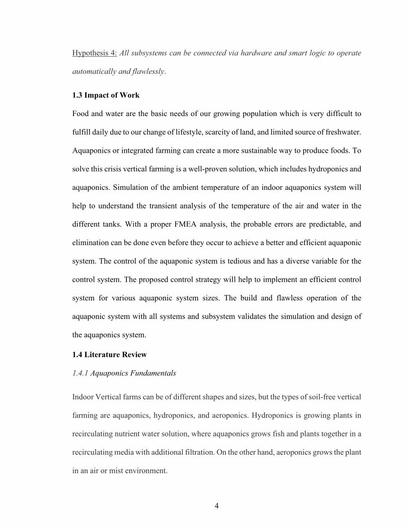
Figure 03: Basic aquaponic system [17].

1.4.2 Approaches

The growth of fish and plants happen in hours or days and are a slow process while

photosynthesis and transpiration in crops happen in seconds or minutes and are fast

processes [18]. As in a closed-loop system, the main water use is due to plant transpiration,

the necessary sizes of system and sub-system depend on plant transpiration. This research

is aiming towards creating an aquaponics simulation and implement it to a physical model

to validate our findings [16]. With the introduction of automation and smart strategies, and

connectivity in the firming industry we can implement them to find a better solution for

the aquaponic system in terms of economic, sustainability, and ease to operate with less

error [19].

1.4.3 Automation

Automation, smart strategies, and connectivity in the farming industry introduce a new era

for the improvement in agriculture [20]. The benefits are expected from smart automation

7

are a considerable decrease in manual labor, better process control by increasing the

accessibility and connectivity of the parameters, and using computer capabilities to make

data-driven decisions [21]. One recurrent type of research in the past years is the

implementation of sensing, smart, or IoT systems in aquaponics to solve some of the

challenges faces by aquaponics growers [22].

Different approaches have been taken by the scientist and researcher to obtain a better and

smart aquaponics system. One of the options is the development of aquaponics system

control locally by using different sensors and connected to a GSM (Global System for

Mobile) communication interface that can send notifications or alarms as per the

predefined set limit [23]. Further modified steps are taken to utilize Arduino and a WRTnod

to monitor the data acquisition and manage the aquaponics system built which gets the data

wirelessly and analyzes then in a cloud server [24]. Our goal is to minimize the overall cost

and hence we will implement a strategy to control the complete system efficiently and

reliably.

1.4.4 Digital Twin (DT)

Digital twins are designed to receive input signals from sensors attached to the physical

object and produce real-time output or feedback that describes how the object would

behave in a virtual environment. The technologies behind digital twins are the internet of

things (IoT) and machine learning, a subset of artificial intelligence (AI) [25]. The IoT

comprises smart, connected devices that interact and exchange information over networks.

Machine learning, on the other hand, refers to statistical models and algorithms that enable

computer systems to carry out specific tasks without acting on any explicit instructions

[26].

8

The basis of interactions of these technologies is to generate data. The data allows

developers to continuously optimize the virtual replica to allow it to adapt to changes to its

real-world twin for days, months, or even years.

1.4.5 Nutrition

Fish waste is the source of the nutrients that are needed for plant growth in the aquaponic

system [27]. Fishes mostly excrete nitrogen (N) in the form of ammonia (NH3) through

their gills [28] although while their waste contains mostly organic (N), phosphorus (P), and

carbon (C) [29][30]. As in aquaponics fish waste is using as a nutrition source so the

nutrients are organic in origin but conventional hydroponic cultivation techniques provide

plants with inorganic nutrients [31]. It has been suggested that nutrients from aquaculture

effluents may not supply sufficient levels of potassium (K), calcium (Ca), or iron (Fe) for

proper plant development, therefore these need to be added as supplements to the system

to ensure optimal plant performance [32][33]. However, adding these supplements requires

closer management of the system and leads to greater costs [34].

Table 01: Nutrients required for plant growth.

9

1.4.6 Other Essential

There are several parameters to have close monitoring for aquaponics and temperature is

one of them. We need to have close control of both air and water temperature. The

temperature in the water is closely related to other water-related parameters. For example,

the optimal temperature for the nitrification process is between 17-34°C [35]. If the water

temperature goes below this range, the productivity of the bacteria will tend to decrease,

and the nitrification process will not be successful. For different fish and plants, the suitable

temperature range is different. Even the higher water temperature resists the plant from

uptake calcium [36]. Air temperature has an important impact on the growth of plants [37].

The suitable temperature for most of the vegetables commonly grown in aquaponics

systems is between 17-34°C [38].

Another important parameter is pH for water solution [39]. As there are three different

living elements in the water fish, microorganisms, and plants and they have a different

range of pH [40]. Although in the hydroponics component the optimum pH is around 6.0.

It has been observed that if pH is higher than 7.0 or lower than 4.5 can cause root injury or

other mineral precipitation [41]. For the aquaponic system, the optimum pH range is

between 6.8 - 7 and the highest possible pH value should be consistent with the prevention

of ammonia accumulation in the system [42].

Dissolved Oxygen (DO) is another important parameter. DO is a measure of how much

oxygen is dissolved in the water available for the aquatic living organisms and is an

important element to support aquatic life [43]. Oxygen is dissolved in water at a very low

concentration and has a drastic effect on the aquaponic system[35]. Dissolved oxygen has

10

a strong relationship with the temperature of water [44]. When the temperature goes up the

amount of dissolved oxygen goes down.

The optimal ratio between fish and plants needs to be identified to get the right balance

between fish nutrient production and plant uptake in each system. This could be based on

the feeding rate ratio, which is the amount of feed per day per square meter of plant varieties

[45]. On this basis, a value between 60 and 100 g day−1 m−2 has been recommended for

leafy-greens growing on raft hydroponic systems [46].

1.4.7 Simulation

Computational fluid dynamics is a numerical tool that is highly accurate to simulate a very

large number of applications and processes. Computational Fluid Dynamics (CFD) is

progressively becoming a design-oriented tool in many engineering fields to solve and

predict engineering problems that involve liquids and gases [47]. CFD has several

attractive features: (a) easy variation of flow parameters, (b) fast changes to the geometry,

and (c) detailed insight into flow behavior. CFD has proven to be accurate and beneficial

in many engineering fields, including aeronautics [48], heat exchanger design [49], cooling

systems [50], and wind turbines [51]. However, few studies have addressed CFD in the

aquaponics system.

1.4.8 Scientific Background

Heat transfer occurs when there is a temperature difference. Heat transfer may occur

rapidly, or slowly. The rate of heat transfer can be controlled by choosing, controlling air

movement, or by choice of color. Heat is usually transferred in a combination of these three

types and seldomly occurs on its own.

11

Equation 1 relates to the heat transferred from one system to another.

Q=c×m×ΔT

…………………………………………………………………………………. (1)

Where,

Q = Heat supplied to the system

m = mass of the system

c = Specific heat capacity of the system

ΔT = Change in temperature of the system

Conduction is heat transfer through stationary matter by physical contact. (The matter is

stationary on a macroscopic scale—we know there is the thermal motion of the atoms and

molecules at any temperature above absolute zero.) Heat transferred between the electric

burner of a stove and the bottom of a pan is transferred by conduction.

Figure 04: Heat transfer of a typical room [52].

Heat transferred by the process of conduction can be expressed by equation 2,

12

Q= kA (THot−TCold)/ t d ………………………………………………………………. (2)

Where, Q = Heat transferred, K = Thermal conductivity, THot = Hot temperature, TCold =

Cold Temperature, t = Time, A = Area of the surface, and d = Thickness of the material.

Convection is the heat transfer by the macroscopic movement of a fluid. This type of

transfer takes place in a forced-air furnace and weather systems. Heat transferred by the

process of convection can be expressed by equation 3,

Q= Hc A (THot−TCold) …………………………………………………………………. (3)

Here, Hc is the heat transfer coefficient.

Radiation is the type of heat transfer that occurs when microwaves, infrared radiation,

visible light, or another form of electromagnetic radiation is emitted or absorbed. An

obvious example is the warming of the Earth by the Sun. A less obvious example is thermal

radiation from the human body. The Heat transferred by the process of radiation can be

given by the following expression,

Q= σ(THot4−TCold

4) A……………………………………………………………………. (4)

Here σ is known as Stefan Boltzmann Constant.

For a mass M of water (specific heat per unit mass Cw) at temperature T in contact with a

heat source at temperature Ts through an area A with a heat transfer coefficient H

(Watt/Kelvin/m2), then the equation 5 of temperature vs time is given by,

dTdt

= (Ts−T)Mcw

HA …………………………………………………………………………. (5)

If we put McwHA

=τ, then the solution for this is of the form equation 6,

13

T=Ts−(Ts−T0) e−t/τ …………………………………………………………………… (6)

The heat transfer coefficient will be a function of the wall construction of the container,

and how well air can flow around it [53][54].

1.4.9 Similar Applications

It is important to determine the dynamics of water and nutrients in the growing substrate

used for soil-less cultivation because this allows better time and space management of the

water and nutrient supply according to plant needs during each step of the crop cycle.

computer fluid dynamics (CFD) software was used to solve the water movement equations

numerically in three dimensions [55]. The development of a root zone cooling system using

a CFD simulation approach to optimize the distance of cooling pipes that can produce the

optimal temperature distribution and uniformity in the planting medium for plant substrate

[56].

Figure 05: Simulation of turbulent kinetic energy distribution [57].

14

Few more attempt has been taken to use to create transient and steady-state models of fish

tanks to visualize velocity profiles, streamlines, and particle movement with the use of

CFD software Open FOAM [58].

1.4.10 FMEA Fundamentals

Standard techniques like Hazard and Operability studies (HAZOP) are conducted by

process and chemical industries to do systematic analysis on a process and its sub-systems

[59]. Failure Mode Effect Analysis (FMEA) is one such tool in a designer’s toolbox and is

recognized as an international standard (IEC 60812), which describes techniques to analyze

processes that can affect the reliability of a process plant or determine what possible

hazards could be present [60]. Many aquaponics operators are not familiar with these

design processes and find design inadequacies after an event, which normally has financial

consequences. This method can find the error in design and process and eventually leads

to identify disturbances that could lead to product deviation and identify hazards for the

aquaponic system [61].

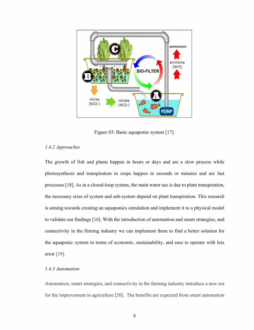
1.4.11 Ever Green- Blue Water Aquaponics system

The Evergreen- Bluewater research lab at Freeman ranch, Texas State University has

indoor vertical farming, and its goal is to find innovative solutions for the global food-

water-energy. This lab has an indoor vertical farm with a complete hydroponic system and

another well insulated 40 ft shipping container for the aquaponics system. The challenge

was to simulate the water temperature for containers inside air and water temperature from

ambient temperature and build a smart automated aquaponics system with less error and

integrate with the existing hydroponic system.

15

Figure 06: Evergreen bluewater shipping container.

16

2. SIMULATION

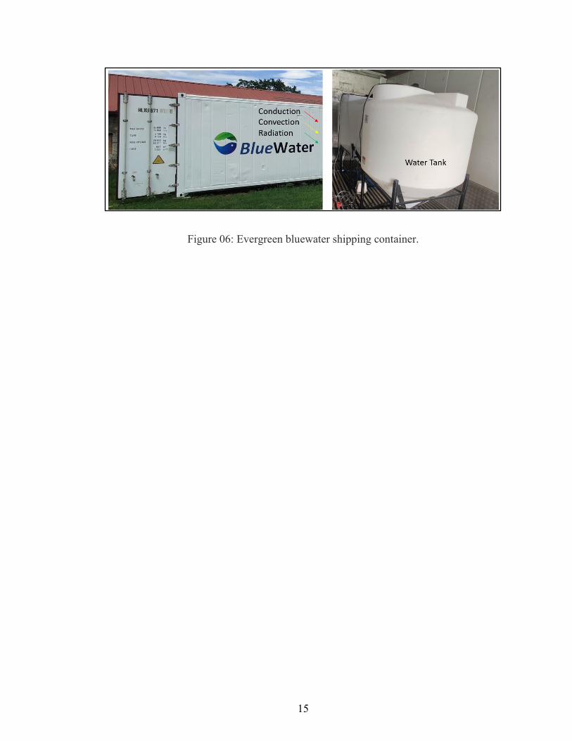
2.1 Introduction and Problem statement

This chapter assesses hypothesis 1: A simulation system can model the ambient

(temperature) of the fish and plant grow areas as well as heating/cooling/gassing

instruments (by considering the outside ambient). To assess this hypothesis, a CFD

simulation was carried out to know the temperature of water and air in the shipping

container for different ambient temperature data. The purpose of the simulation is to know

the temperature for design the aquaponics system including water and air chiller, heater

even to select the right species and size of fish and plant.

2.2 Methods and Materials

The heat is from the ambient or outside was transferred to the water tanks in three steps.

First, heat transfer to the wall of the shipping container by solar radiation, then heat

transfers from the wall to the inside air, and finally, heat is transferred from the container

inside air to water. The complete setup of the shipping container with the water tank was

modeled with Comsol Multiphysics® software [62]. The simulation was following few

basic steps:

1. Drawing and setting up the geometry of all components.

2. Setting up the initial and boundary conditions.

3. Adding physics and multiphysics to the model to link all the heat transfer phenomena.

3. Creating and building mesh.

4. Creating time-dependent study with multiphysics.

17

5. Running the simulation and analyzing the result.

Figure 07: Steps to follow in simulation.

2.3 Geometrical Modeling

To start the simulation the full system was converted to a CAD model with actual

dimensions. The actual dimension was measured from the actual model in the freeman

center.

Figure 08: Indoor aquaponic system.

The water tanks are added to the model. All major components including container wall,

air, water, and water tanks are defined properly.

18

Figure 09: Shipping container geometry.

The shipping container offers many benefits to choose for an indoor aquaponics system.

They are mobile, which means the farm can move wherever required and can be placed

nearby the city area to minimize the food miles.

Figure 10: Shipping container cross-section.

The dimension of the shipping container is length 40 feet, width 8 feet, and height around

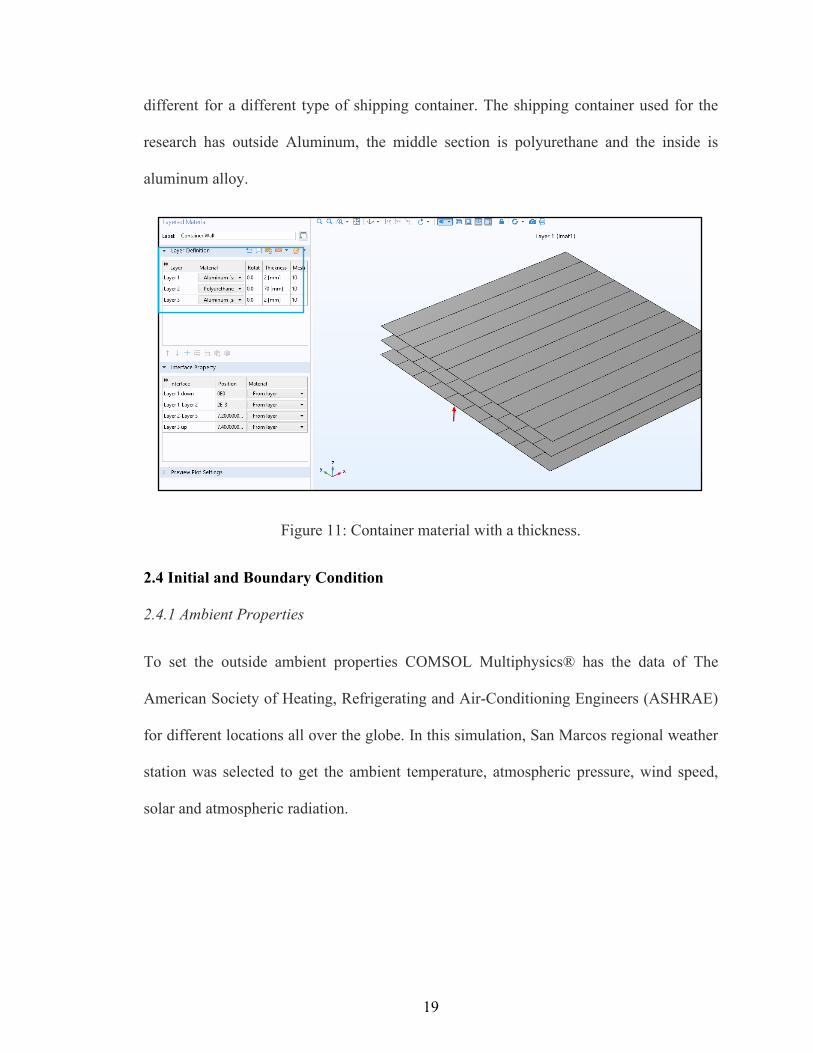
9 feet. The shipping container is a combination of three-layer of materials. The material is

19

different for a different type of shipping container. The shipping container used for the

research has outside Aluminum, the middle section is polyurethane and the inside is

aluminum alloy.

Figure 11: Container material with a thickness.

2.4 Initial and Boundary Condition

2.4.1 Ambient Properties

To set the outside ambient properties COMSOL Multiphysics® has the data of The

American Society of Heating, Refrigerating and Air-Conditioning Engineers (ASHRAE)

for different locations all over the globe. In this simulation, San Marcos regional weather

station was selected to get the ambient temperature, atmospheric pressure, wind speed,

solar and atmospheric radiation.

20

Figure 12: Setting of ambient conditions.

To run the simulation the start data was selected from 5/15/2021 for 72 hours. The initial

temperature of the inside air of the shipping container was selected as 25⁰C.

Figure 13: Selection of date and time.

2.4.2 Azimuthal

The actual azimuthal of the container was measured and use in the simulation software.

The azimuth measures the angular distance of the object east from north and parallel to the

21

observer's horizon. Along with the altitude, the azimuth of an object is used to define its

position on the celestial sphere in the horizontal coordinate system.

Figure 14: CAD model and azimuthal of the shipping container.

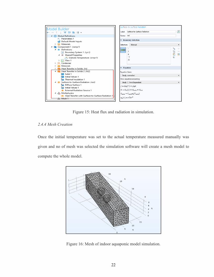
2.4.3 Physics and Multiphysics

The heat from the ambient or outside was transferred in three steps.

1. Heat transfer at the wall of the shipping container

2. Heat transfer from the wall to the inside air

3. Heat transfer from the container inside air to water.

For this study, two physics was considered. One is for conduction and convection and

another is for surface-to-surface radiation.

22

Figure 15: Heat flux and radiation in simulation.

2.4.4 Mesh Creation

Once the initial temperature was set to the actual temperature measured manually was

given and no of mesh was selected the simulation software will create a mesh model to

compute the whole model.

Figure 16: Mesh of indoor aquaponic model simulation.

23

2.4.5 Time-Dependent Study

A time-dependent study was set up for the simulation. The time unit was in an hour, the

output time range was 0.5 hours, and run for 72 hours. The compute was done for the

simulation and it took around 10 minutes to run the computation.

Figure 17: Time step for simulation

2.5 Result

After the simulation was carried out the result section produced simulated data based on

the outside ambient data. The solar irradiance on the shipping container is shown for a

different period. This simulation was carried out for 72 hours. The arrow indicates the solar

irradiance from the sun to the surface of the shipping container.

24

Table 02: Solar irradiance on the shipping container.

From table 02 we can see that how the ambient temperature affects the container surface,

air, and water. For example, in the morning 0800 hrs. the roof is not that hot compared to

1200 hrs. At night 2200 hrs. there is no solar irradiance.

From the result section of simulation software, we can generate a lot of different transient

analyses of individual surfaces, the volume of different geometry. As our target is to know

the water temperature of the water tank kept inside the shipping container. So, in figure 18

we plot the simulated temperature for 72 hours.

25

Figure 18: Simulated temperature vs time in the result section.

From figure 18 we can see that, inside water temperature is not influenced that much by

the outside air temperature. But there is very little change in water temperature because

there was no external heating source (lights) in the system, and it needs a significant amount

of heat to change the temperature of 300 gallons of water.

2.6 Validation

To validate the simulation few temperature loggers were used to get the actual temperature

of the water, the air inside the shipping container. The outside temperature data was

gathered from the weather station of the freeman ranch, situated nearby the shipping

container. This temperature was gathering and plotted to compare with the simulation data.

A sample data table is listed in appendix A-1.

26

Figure 19: Measuring actual temperature with a temperature logger.

The temperature data logger (Elitech GSP-6G) ® [63] was used which can measure and

store the temperature of air and water every 15 minutes and can record up to 16000 records.

It has a wide temperature measurement range from -40℉ to 185℉, max with accuracy up

to ±0.5℉.

Figure 20: Comparison between actual and simulated temperature.

27

Figure 20, describing that the temperature data from the simulation and the actual data are

almost matches with each other except at times where there is a very little deviation.

Figure 21: Statistical analysis of actual and simulated temperature.

From figure 21, the paired T-test with a 95% confidence interval showed that the simulated

data and actual temperature data are almost similar. The possible reason for this deviation

is that the actual condition cannot be considered properly in the simulation model or there

could be small leakage of air that can lead to error.

2.6.1 Additional Scenarios

Once the model is validated in the simulation additional water tank was added to check the

temperature profile. The additional water tank is of the same dimension and materials.

28

Figure 22: Adding a third tank for simulation.

From figure 22, the third water tank was added with the existing model, and the mesh has

been created. With the same date and initial and boundary condition, the simulation was

computed to get the average temperature of three water tanks and compared with the

existing result for two water tanks.

Figure 23: Comparision between 3 water tanks and 2 water tanks simulated temperature.

From figure 23, the comparison of simulated temperature between 3 water tanks and 2

water tanks is plotted and found that the temperature is almost the same even with an

addition of a water tank.

29

Figure 24: Simulated temperature of water and air of typical winter days.

Figure 24 represents a simulation for 72 hours of two water tanks during a typical winter

season. The initial temperature for air and water was considered 10 °C and during the

period the change of ambient temperature creates a good amount of change in the air

temperature but the water temperature remains more steady. It is understandable from the

simulated water temperature profile that, during this time the water heater will remain

operational and the specification of heating capacity can be selected for a certain type of

fish of any aquaponics.

2.7 Conclusion

From the simulation, it was observed that the actual temperature and simulated temperature

are almost similar for any given amount of water. From the paired T-test between actual

and simulated temperature, we found that there was no statistically significant difference

between them and accepted the claim of hypothesis 1. The suitable type and number of

fish and species can be decided for the indoor aquaponics setup based on the computer

30

model. With the simulation of temperature, it is easy to design the cooling and heating

instrument and their necessary setup for the smooth operation.

31

3. FAILURE MODE AND EFFECT ANALYSIS

3.1 Introduction and Problem Statement

This chapter assesses hypothesis 2: Aquaponics design and operations can be more

accurate. Many mistakes can be preventable before it happens by the FMEA. Many

mistakes can be preventable before it happens by the FMEA method. FMEA can be used

at various steps in a design process to identify issues that can affect the reliability of the

process. Ideally, a group of multifunctional engineers or designers that have skill sets in

various disciplines could carry out the FMEA. Identifying weaknesses in a process design

early in the concept and design phase of the project can allow engineering controls to be

implemented long before the process is operational. The score identifies areas that can be

of concern and where engineering controls could be implemented to prevent or mitigate

the identified systems or subsystems of the process. The engineering controls do not

necessarily need to be automation controls but could be in various other forms such as

additional engineering reviews or mitigating hazards by alternate design.

O – the probability of occurrence, S – the severity of occurrence

D – the probability of detection

Figure 25: (a) Functions of FMEA (b) Scoring system [64].

32

3.2 Methods and Materials

FMEA is generally used for analyzing new designs or processes, modifying an existing

product design or process, and using a design or process in a new environment. It is usually

recommended to use FMEA periodically throughout the life span of a product or service.

FMEA can be of many types, still, it is divided into two main groups. For evaluating any

process, it is known as PFMEA and for any design, the FMEA is known as DFMEA.

Usually, a group of experts of that different sector forms a team to conduct the FMEA. The

FMEA review results are documented in a table to record any responses and to determine

the RPN score. Design notes were also taken at this stage as the analysis also identified

possible design solutions. Recording the outcomes of the analysis will aid in the design

process as it allows validation data to be collected that can be referred to for verification as

the design develops.

Figure 26: Process of FMEA analysis [65].

To conduct the FMEA analysis for the indoor aquaponics system the process flow chart is

considered as the basic document to learn about the design and process. The steps required

to conduct FMEA are described below:

33

Figure 27: FMEA for aquaponics.

STEP 1: Review the process

A process flow chart for PFMEA or details design documents for DFMEA is considered

as the base document for FMEA. For the indoor aquaponic system one general FMEA

analysis is prepared. For this FMEA the process flow chart was used to identify each

process component.

Figure 28: Process flow chart.

34

As aquaponics has lots of variables so the overall process is divided into subcategories like

mechanical, Electrical, Physical, Nutrition, and Data.

Figure 29: Subsystem of FEMA of aquaponics.

For each system, there are several subsystems. For example, the mechanical system is a

combination of several mechanical components like water tanks, biofilter tanks, pipe and

hose, the growing rack, and many others. For this research, the most important components

are considered.

STEP 2: Brainstorm potential failure modes

To identify the potential failure, it is necessary to know about the design and function of

that item. For example, the mechanical item has some specific requirements, and this

requirement will help to evaluate the severity of any failure that happened for that item.

This list of failures is from the expertise of the team member or review existing

documentation and data for clues about all the ways each component can fail. There will

likely be several potential failures for each component.

35

Table 03: Item, function, and requirement for any aquaponics FMEA.

From table 03 for the mechanical system, one of the items of that system pipe was shown.

The necessity of the pipe and its requirement for the aquaponic system were listed. The

possible failure of the pipe could be broken, clogged, algae were grown or degraded.

STEP 3: List potential effects of each failure

The effect is the impact the failure has on the product or subsequent steps in the process.

There will likely be more than one effect for each failure. For example, from figure 26 the

effect of a particular failure mode of the pipe may affect the disturbance of the flow of

nutrient-rich water from the fish tank to the plant.

36

Figure 30: Effect of the failure mode.

STEP 4: Assign Severity rankings

The Severity Ranking is an estimate of how serious an effect would be if it occurs. Based

on the severity of the consequences of failure the severity for that specific failure is ranked

between 0 to 10. In this research for any failure that can kill the fish or plant is considered

most severe and ranked accordingly.

Figure 31: Severity for that failure.

37

STEP 5: Assign Occurrence rankings

The occurrence ranking is based on the possibility of regularity that the cause of failure

will occur. Once the cause is known to the team the data was captured on the frequency of

the cause. For example, for the pipe leakage, the cause can be an improper joint between

the pipe and hose, and the chance to repeat the problem is 3 out of 10. As the chance of

repeat is lower so the raking is lower too.

Figure 32: Occurrence for that failure.

STEP 6: Assign Detection rankings

To assign detection rankings, we need to identify the process or product-related controls in

place for each failure mode and then assign a detection ranking to each control.

Table 04: Occurrence ranking for any failure.

38

Detection rankings evaluate the current process controls in place. A control can relate to

the failure mode itself, the cause (or mechanism) of failure, or the effects of a failure mode.

To make evaluating controls even more complex, controls can either prevent a failure mode

or cause from occurring or detect a failure mode, cause of failure, or effect of failure after

it has occurred.

Figure 33: Detection for any failure.

STEP 7: Calculate the RPN

RPN gives us the relative ranking between the errors. It is calculated by multiplying three

rankings together. After calculating all the RPN for all the failures the priority was set up

according to the RPN value. The more the RPN the most critical that failure is.

Figure 34: RPN for any failure.

STEP 8: Develop the action plan

39

Once the RPN is calculated and the highest RPN will get focus and taken care of first. The

next step is to assign someone for mitigation of that specific error.

Action Recommended

Responsibility

Action Taken

What are the recommended actions for reducing the occurrence of the cause or improving detection?

Who is responsible for making sure that the actions are completed?

What actions were completed (and when) for RPN?

Figure 35: Responsibility for the defined actions.

STEP 9: Actions Taken

Implement the improvements identified by the FMEA team. The Action Plan outlines what

steps are needed to implement the solution, who will do them, and when they will be

completed. Most Action Plans identified during a PFMEA will be of the simple “who,

what, & when” category. Responsibilities and target completion dates for specific actions

to be taken are identified.

Action Recommended

Responsibility

Action Taken

What are the recommended actions for reducing the occurrence of the cause or improving detection?

Who is responsible for making sure that the actions are completed?

What actions were completed (and when) for RPN?

Figure 36: Action is taken to reduce the RPN.

40

STEP 10: Calculate the resulting RPN

Re-evaluate each of the potential failures once improvements have been made and

determine the impact of the improvements. This step in a PFMEA confirms the action plan

had the desired results by calculating the revised RPN. To recalculate the RPN, reassess

the severity, occurrence, and detection rankings for the failure modes after the action plan

has been completed.

Figure 37: Re-evaluate RPN.

3.3 Improvement in Aquaponics

In this research, a complete FMEA was carried out for Evergreen-Blue water aquaponics

at the Freeman Ranch and a few of the important improvements with RPN are listed below:

41

Table 05: Improvements in aquaponics.

System Improvements RPN Before After

Mechanical

Cause of failure: Leakage in hose connection. Prevention: Eliminate improper joints or the addition of clamps in the high-pressure regions.

60

20

Physical

Cause of failure: Bubble from air pump was uncontrolled. Prevention: Put a control valve after the air pump.

90

40

Electrical

Cause of failure: Electrical relay was not placed properly causing an automation error. Prevention: Secured the relay with support for smooth operation.

80

30

The FMEA chart was divided into sub-systems like mechanical, electrical, physical and

nutrition, and data. For all subsystems, the list was constructed. As the aquaponics system

in this research is in the development phase so, mostly the list focuses on design and

process improvement.

Figure 38: Improvement of water hose clamping before any leakage.

42

Figure 39: Improvement of electrical system before any error during operations.

Figure 40: Improvement of a physical system before it harms the fishes.

3.4 Results

This research is based on the general FMEA for the indoor aquaponic system and one

complete FMEA is listed in appendix B. The ultimate target of the FMEA is to reduce the

failure and before it happens or improve the process for not happen further. The RPN is

the numerical value calculated to identify the weight of that failure and its impact. The

43

FMEA list prepared and necessary actions taken by the concerned team can improve the

RPN and hence improve the overall design and process.

Figure 41: Improvement with FMEA.

3.5 Conclusion

In this research, the application of FMEA helps the design, build, and operation of the

aquaponic system more errorless and it showed clearly with reduction of risk priority

number. Hence the claim of hypothesis-2 is accepted.

FMEA is a lean six sigma tool used to mitigate the risk of possible failures. FMEA needed

to be done at the design stage, operation stage and throughout the life span of the aquaponic

system and update the list and use as future references for the future grower. Although

FMEA has many advantages, still there are few limitations and different improvements

done so far to make it more reliable. As the risk priority no is based on the judgment of the

responsible person and team, there is always a chance of human error. If the risk priority

no became the same for few errors, then the priority setting might be a little confusing for

the user. Updated FMEA like fuzzy FMEA and Logistic regression-based FMEA can be

used to eliminate the possible error.

44

4. SMART AUTOMATION


This chapter assesses hypothesis 3: Aquaponics operation and feeding mechanism can

be optimized. Correlation between instrument settings (e.g., pump flow,

heat/cooling/gassing hrs., and feeding setting) and by considering outside ambient can be

found that maintain the system near optimum conditions. The major challenge of the

aquaponic system is the initial investment and the operation cost. The operation is labor-

intensive and requires an expert operator. This chapter is focused on the development and

implementation of automation and make the system less costly to operate. The

microcontroller-based control system and digital twin are utilized to predict and control the

system with less error and greater output.

4.2 Method and Materials

The control an automated aquaponic system many parameters need to be measured and

controlled. Plants and fish in the system each have a feasible range and a desirable point

for each of these parameters. If the condition falls outside of the feasible range (e.g., water

temperature too hot), it will be fatal to these creatures. To operate an aquaponics control

system, all parameters should be identified, the feasible range of each parameter for the

plants and fish should be determined, measured, and adjusted. Each living element has a

different range or limit of parameters based on species. So, while selecting the type of fish

and plants the temperature range is a serious concern. For this complex system, the

proposed solution is to separate the control paraments into two different categories. Level-

01 are those parameters directly related to the life of fish, plants, or microorganisms. This

continuous monitoring will be carried out by measuring temperature, Dissolved Oxygen,

45

pH, and nitrate of the water solution by using sensors and microcontroller-based computing

systems. Level-02 are those parameters needed to monitor periodically for the smooth

growth of the aquaponic system. Handheld meters or sensors will be used, and the data will

be recorded in a computer or any mobile application and verified with reference data. For

level-02 monitoring, the nutrition level, total dissolved solids (TDS), electrical

conductivity (EC), and total ammonium nitrate (TAN) of water solution are recorded.

Figure 42: Automatic control of aquaponics system.

4.2.1 Temperature Control

Each plant and fish species have a level of tolerance and an optimum point for ambient

temperature. The suitable temperature range for most vegetables is 18 - 30 ⁰C [66].

Although few vegetables like lettuce and cucumbers like temperature 8⁰C – 20 ⁰C and some

vegetables like okra, basil suited a temperature range between 17⁰C – 30 ⁰C. Fishes are

cold-blooded and can't survive with a big temperature range. For fishes like tilapia and

46

catfish, they survive around 22 – 32 ⁰C. Other cold-water fishes like to have a range of

temperature between 10 – 18 ⁰C. For microorganisms like nitrifying bacteria, the ideal

temperature range should be around 17 – 34 ⁰. To get a feasible condition for all living

elements in the system, the temperature setting is set between 18- 30 ⁰C [67].

Figure 43: Temperature range for all living elements in aquaponics.

To keep the system temperature within the range, the temperature was measured with a

DS18B20 temperature probe. The probe is submerged into water and based on the reading

the microcontroller is deciding to on or off the water chiller or heater to achieve a controlled

temperature.

Figure 44: Temperature control logic for an aquaponic system.

47

4.2.2 pH Control

Another important parameter that needs to regulate is pH for water. As there are three

different living elements in the water fish, microorganisms, and plants and they have a

different range of pH [40]. Although the hydroponics component of the aquaponics system

has the optimum pH requirement is slightly acidic (5.5-5.8) [68]. If the pH became higher

than 7.0 or lower than 4.5 the plats may have root injury or other mineral precipitation on

the plant roots may hamper the intake of the mineral [41]. On the other hand, fish can

tolerate a wider pH range. The optimal pH for fishes is different for different fish species.

For nitrification, the pH range for optimum performance of nitrifying bacteria is between

7.5 -8 [68].

Figure 45: pH range for all living elements in aquaponics.

For the aquaponic system, the overall optimum pH range is between 6.8 - 7. To control the

pH fluctuation first pH was measured with Atlas scientific pH probe connected with a

microcontroller. With a pre-set pH range between 6.8 -7, the microcontroller will operate

a pH increase or reducing chemical dosing pump.

48

Figure 46: pH control logic for an aquaponic system.

4.2.3 Dissolved oxygen

Dissolved Oxygen (DO) is another important parameter for aquaponics. DO is a measure

of how much oxygen is dissolved in the water available for aquatic living organisms.

Oxygen is dissolved in water at a very low concentration and has a drastic effect on the

aquaponic system [69]. Dissolved oxygen has a strong relationship with the temperature of

the water. When the temperature increased the amount of dissolved oxygen goes down

[67]. DO level was measured with Atlas scientific DO sensor and the microcontroller will

operate the air blower to increase the DO level. The general recommendation for DO level

for the aquaponic system is a minimum of 5 PPM (Parts per million) [70]. When the DO

level is going down the fish will try to come on the water surface. One Atlas scientific DO

sensor has been used to measure the level of DO in water. Once the Level is going down

below 5 PPM, the aeration motor will be starting and will increase the DO to maintain a

certain level of DO in water.

49

Figure 47: DO control logic for an aquaponic system.

4.2.4 Nitrate

Nitrate is a very important parameter for an aquaponics system. Fish waster and leftover

fish food will be converted to un-ionized ammonia (NH3) and ionized ammonium (NH4+).

Un– ionized ammonia is toxic to fish. The total value of ammonia and ammonium is called

total ammonium nitrate (TAN) [71]. To measure the TAN a lot of commercial methods are

available. Nitrification is the process to convert toxic ammonia into nitrate (NO3) with the

help of nitrification bacteria. The nitrate level should be less than 90 mg/L for a healthy

aquaponics system [40]. The plant will uptake the nitrate from the water as a nutrient. In

this research, one nitrate sensor with a microcontroller has been used the measure the

amount of nitrate and manipulate the fish food amount and type to controller the overall

nitrification system of the aquaponic system. The overall nitrate level is recommended

between 50-100 mg/L [72].

Figure 48: Nitrate control flowchart for an aquaponic system.

50

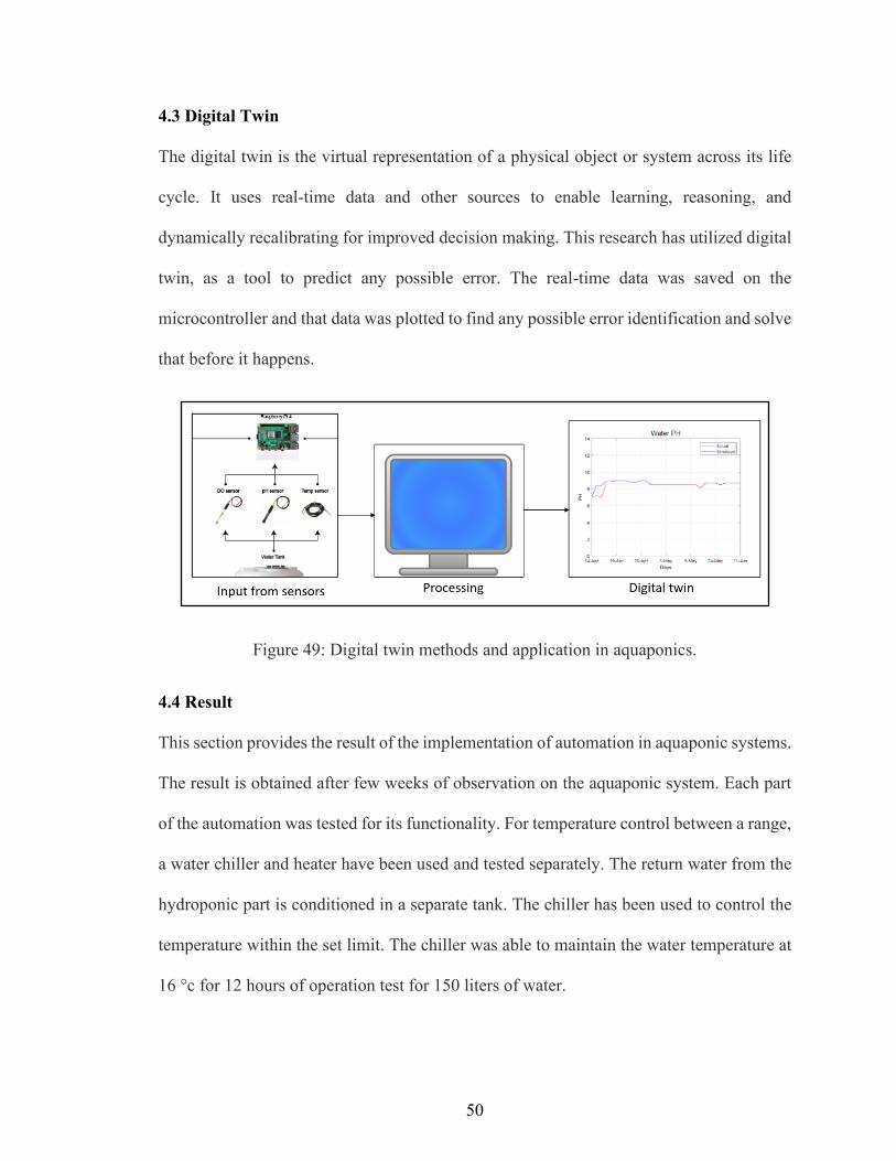
4.3 Digital Twin

The digital twin is the virtual representation of a physical object or system across its life

cycle. It uses real-time data and other sources to enable learning, reasoning, and

dynamically recalibrating for improved decision making. This research has utilized digital

twin, as a tool to predict any possible error. The real-time data was saved on the

microcontroller and that data was plotted to find any possible error identification and solve

that before it happens.

Figure 49: Digital twin methods and application in aquaponics.

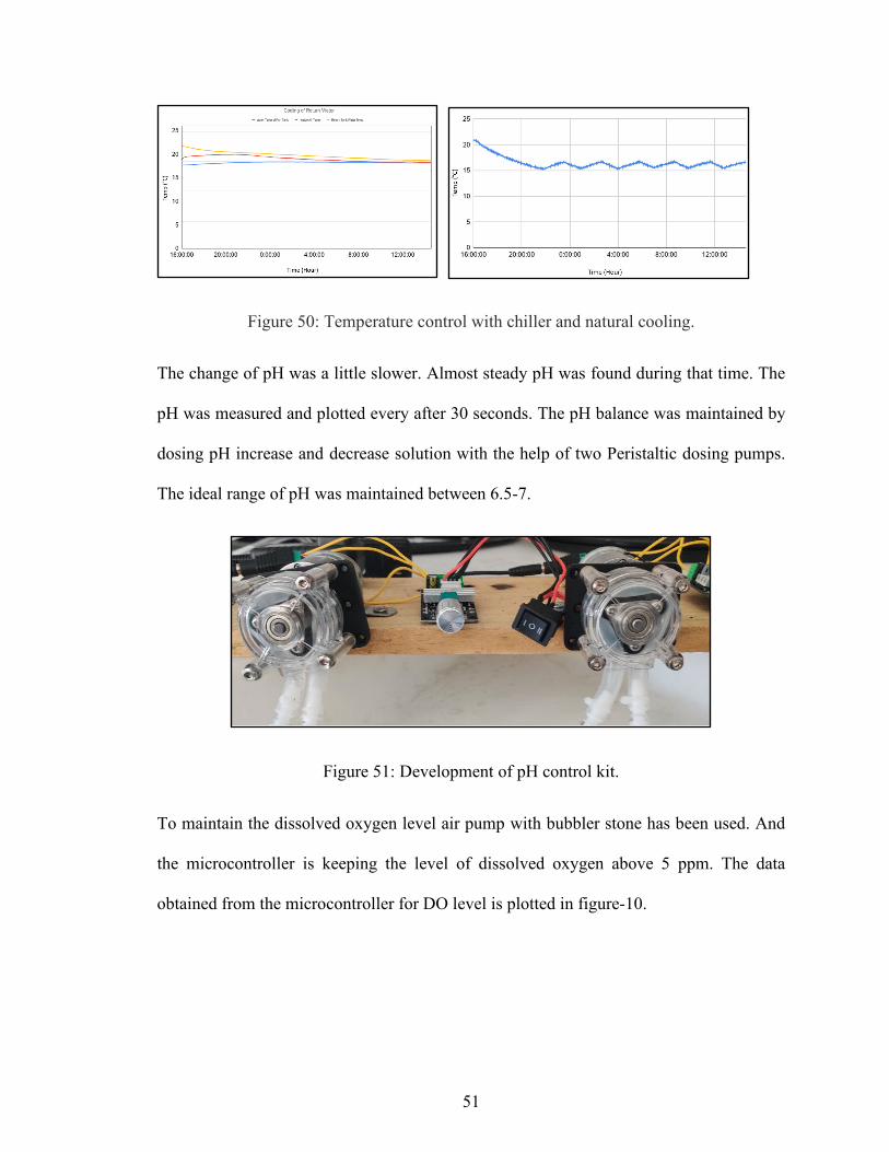
4.4 Result

This section provides the result of the implementation of automation in aquaponic systems.

The result is obtained after few weeks of observation on the aquaponic system. Each part

of the automation was tested for its functionality. For temperature control between a range,

a water chiller and heater have been used and tested separately. The return water from the

hydroponic part is conditioned in a separate tank. The chiller has been used to control the

temperature within the set limit. The chiller was able to maintain the water temperature at

16 °c for 12 hours of operation test for 150 liters of water.

51

Figure 50: Temperature control with chiller and natural cooling.

The change of pH was a little slower. Almost steady pH was found during that time. The

pH was measured and plotted every after 30 seconds. The pH balance was maintained by

dosing pH increase and decrease solution with the help of two Peristaltic dosing pumps.

The ideal range of pH was maintained between 6.5-7.

Figure 51: Development of pH control kit.

To maintain the dissolved oxygen level air pump with bubbler stone has been used. And

the microcontroller is keeping the level of dissolved oxygen above 5 ppm. The data

obtained from the microcontroller for DO level is plotted in figure-10.

52

Figure 52: pH and DO level output graph.

The nitrate level has been controlled by controlling the types and amount of fish food. As

nitrate is the result of the nitrification process, so the increased amount of nitrate indicates

the under-designed biofilter and will be harmful to the aquatic living condition. The level

of ammonia is needed to measure regularly. One portable Ammonia sensor was used to

measure the ammonia and can be manipulated by changing the fish water or increasing the

biofilter size or the number of plants, or the number of fish. It's always recommended not

the change all water at a time for the aquaponics system.

Figure 53: Power consumption per hour and monitoring for aquaponics.

The power consumption was measured manually with a digital power measuring tool and

plotted the consumption to monitor the activity of the system.

53

Figure 54: pH monitoring and application for Digital Twin.

Once, data from raspberry pi was transferred and plotted to prepare a digital twin of the

system. With any gradual change in the trend of data, the prediction of possible error with

digital twin can be possible. Any aquaponic grower can eliminate errors from the system

before they happen.

4.5 Discussion and Conclusions

The claim in hypothesis 3 is accepted as the design, installation, coding, and application of

automation for the aquaponic system replaced most manual activities and the digital twin

brought a real-time monitoring experience. In this research, for the automation, the major

challenge was the integration of different sensors for the microcontroller and controlling

the flow rate with different pumps. For the limitation of nitrate sensor one Arduino-based

controller use used for the control of nitrate. The ammonia sensor is required that can

measure and integrate with the microcontroller is one of the future tasks. As these, sensors

are monitoring the data continuously, another challenge is to calibrate the sensors to ensure

data accuracy.

54

5. EMPIRICAL STUDY: INTEGRATED SYSTEM IN OPERATION


This chapter describes hypothesis 04: All subsystems can be connected via hardware and

smart logic to operate automatically and flawlessly.

To verify this hypothesis, one complete aquaponic system was developed from design to

operation. Microcontroller-based smart automation and monitoring system was deployed

for the smooth operation of the system. The system ran and was monitored for a long period

with living fish to demonstrate the accuracy and consistency of the system.

5.2 Method and Materials

The aquaponic system was developed through a standard product development

process. Product development steps vary based on the nature of the product requirement

and business strategy, but most products and process development follow these main steps

in the development process.

Figure 55: Product development steps.

Concept Generatioon

Selection

Design Finalization

Fabrication

Testing

55

5.2.1 Concept Generation

A literature review is the first step of concept generation. As this is not a new product so

in the market there is already developed commercial aquaponics system. To adjust the

system with existing hydroponic set up the necessary consideration was made, like water

tank size selection, water transfer method, pump selection. To understand the basic

operation of an aquaponic system one desktop commercial mini aquaponic setup was

collected and observed the system to plan the operation process of the aquaponic system.

Figure 56: Mini aquaponics for process study.

5.2.2 Selection of Components

To find out the required components for the aquaponics system the process layout was

created and with the process diagram the actual dimensions are taken from the research

containers and the Bill of materials was developed.

56

Figure 57: The process plan for the aquaponics system.

Once the process was developed the next step is the break the process into a system and

sub-system. The aquaponic is divided into mechanical, electrical, and control subsystem.

Figure 58: System and subsystem of aquaponics.

System

Electrical Mechanical Control

57

5.2.3 CAD model

Once the system and sub-system were defined then the entire model was developed into

CAD software and that verifies the dimension to prepare the bill of materials.

Figure 59: CAD model of aquaponics.

5.2.4 Mechanical System

The mechanical system is consisting of the following components:

Tanks

300-gallon cone bottom plastic tank is manufactured from linear polyethylene in one-piece,

seamless construction, this tank series is designed for storage applications. UV stabilized

for outdoor usage. One of the tanks was used for fish raising and another is used for the

treatment of water that returned from the plant side.

58

Figure 60: Water tank and biofilter.

Pumps

To transfer the water between the tanks and container few submersible pumps were

used[73]. The water flow rate can be manipulated with the control manual control valve.

Figure 61: Water transfer pump

Specification of the pump:

1. 550 gallons per hour

2. Indoor / outdoor use

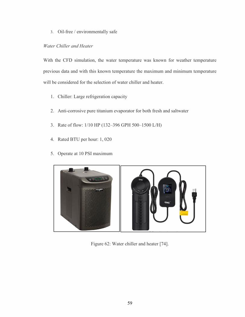
59

3. Oil-free / environmentally safe

Water Chiller and Heater

With the CFD simulation, the water temperature was known for weather temperature

previous data and with this known temperature the maximum and minimum temperature

will be considered for the selection of water chiller and heater.

1. Chiller: Large refrigeration capacity

2. Anti-corrosive pure titanium evaporator for both fresh and saltwater

3. Rate of flow: 1/10 HP (132‒396 GPH 500‒1500 L/H)

4. Rated BTU per hour: 1, 020

5. Operate at 10 PSI maximum

Figure 62: Water chiller and heater [74].

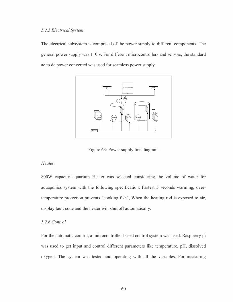
60

5.2.5 Electrical System

The electrical subsystem is comprised of the power supply to different components. The

general power supply was 110 v. For different microcontrollers and sensors, the standard

ac to dc power converted was used for seamless power supply.

Figure 63: Power supply line diagram.

Heater

800W capacity aquarium Heater was selected considering the volume of water for

aquaponics system with the following specification: Fastest 5 seconds warming, over-

temperature protection prevents "cooking fish", When the heating rod is exposed to air,

display fault code and the heater will shut off automatically.

5.2.6 Control

For the automatic control, a microcontroller-based control system was used. Raspberry pi

was used to get input and control different parameters like temperature, pH, dissolved

oxygen. The system was tested and operating with all the variables. For measuring

61

Ammonia one stand-alone sensor was used. From both containers, the data will be transfer

towards a central raspberry pi and it will be stored in a local server.

Figure 64: Data transfer plan.

5.2.7 Coding

Python was used to write the code for the raspberry pi control part. The detail’s code was

listed in the appendix- C1 section. For the Arduino control part, the code was written in

Arduino's built-in system. The detail’s code for nitrate and fish feed control is in Appendix

C 2.

Figure 65: Temperature control logic and flow diagram for the aquaponics system.

62

Figure 66: Sample code for automation.

5.2.8 Sensors

Temperature sensor: To measure the temperature of the fish tank and return water

tank two temperature sensor from Atlas scientific® PT-100 was used [75]. The

specification of the sensors is given below.

Figure 67: Temperature sensor.

63

pH sensor: To measure the pH of the return water one pH sensor from Atlas

scientific® was used. The detailed specification of the sensors is given below.

Figure 68: pH sensor [76].

Dissolved oxygen: To measure the dissolved in both fish tank and returned water tank

two dissolved oxygen sensors were used.

Figure 69: Dissolved oxygen sensor [77].

Nitrate: To measure the nitrate of the aquaponics system, one nitrate sensor from

vernier was used. It can measure nitrate between 1 to 14000 mg/Liter (PPM).

64

Figure 70: Nitrate sensor [78].

Ammonia: Seneye® sensor monitors the highly toxic free ammonia (NH3) at very

low levels. That helps to prevent fishes dying from Ammonia poisoning. The only

drawback of that sensor is it has to connect to a desktop computer.

Figure 71: Ammonia sensor [79].

5.3 Result

From the automation, with the microcontroller, the sensors are operating, and based on the

preset value it can operate different equipment to control the parameters like Dissolved

oxygen, pH, Temperature, etc. The Seneye® sensor is giving the result in the connected

web application. It is an integrated sensor with Temperature, pH, and Ammonia.

65

Figure 72: Ammonia integrated sensor.

From figure 68, the parameters like temperature are 28 ⁰C, pH is 6.89, and ammonia is

0.080 mg/L. The chiller was operated as per temperature logic.

Figure 73: Live fish in the aquaponics system.

Figure 70 describing the fluctuation of temperature in the container but the water for the

fish tank is much steady.

66

Figure 74: Chilled water and air temperature vs time.

The dissolved oxygen level has a strong relation with temperature. If the temperature of

the water is getting higher the dissolved oxygen level is going down, on the other hand, if

the temperature is getting down the dissolved oxygen is going high.

Figure 75: Steady dissolved oxygen level for varying temperatures.

67

From figure 70 it is proven that with a variation of the container inside temperature the

water temperature is steady with the automatic operation of the water chiller according to

logic. From figure 71 is it clear that with a temperature variation the dissolved oxygen level

is quite steady that validates the integrity of the system and its automation.

5.4 Conclusion

The claim in Hypothesis 4 is accepted by design, build and operate the aquaponic system

with fish for a long period. With the help of a process diagram, the overall process can be

assessed and the programs for automation can be scripted. The integration of all systems is

tedious and needed expert guidelines for different parameters. As the fish and plant grow

with time and the setting of many parameters like fish food quantity needed to be adjusted.

It was tough in this research to integrate the ammonia sensor with the main automation,

although ammonia is a very critical parameter. A standalone sensor with an internet

connection can be possible to remotely manipulate the ammonia content by taking out a

certain percentage of water from the fish water tank and add the same amount of freshwater.

68

6. CONCLUSION AND DISCUSSION

Proper planning is the key to success for design, build and operate an aquaponics system.

With the help of simulation, the water temperature in the fish water tank was available for

any period from past ambient data. The suitable type and number of fish and species, the

design of the cooling and heating instrument, and their necessary setup for the smooth

operation were decided for the indoor aquaponics. The aquaponic system design and

operations became more errorless with the application of FMEA. FMEA needed to be done

at the design stage, operation stage and throughout the life span of the aquaponic system

and update the list and use as future references for the future grower. Smart automation

helps to operate the aquaponics system flawlessly without the presence of many operation

personal. The application of the digital twin brought a real-time monitoring experience and

helped to prevent any possible error by observing the trend of parameters. During the

development of the aquaponics system, the process diagram and a proper bill of materials

helped to prevent delays in logistics and scripting of the program for microcontrollers.

Operation of the aquaponic system with fish for a longer period with automation and digital

twin helps to validate the hypotheses for this research.

Future Works

During the research few observation was listed that might be helpful for future

improvement of the aquaponic system:

1. For simulation of the ambient condition, there is a dependency on the historical weather

data. As the simulated parameters will be used for the future, the dependency on the

69

previous data may lead towards the wrong design of the complete aquaponics system if

there is any wrong in consideration.

2. The automation developed in this research cannot be integrated into a single automation.

The ammonia sensors available in the market were found not integrated with the

microcontroller. The existing standalone sensor can be integrated with image processing

tools to integrate with existing automation.

3. The developed automation is connected with wires and looks messy. The operation area

is not clean enough for the operators to work freely. Wireless sensors and IoT relay can be

used for automation.

4. The implementation of the digital twin is still offline for this research. As sensors are

connected it is quite possible to make it a real-time digital twin with the help of internet

connectivity.

5. The overall system can be more optimized with better-integrated planning and

development time cant be reduced with the help of any project management software.

70

APPENDIX SECTION

APPENDIX A: Experimental data log

Table A-1: Sample table for temperature reading for validation of simulation.

71

APPENDIX B: FMEA

Table B-1: Full FMEA table for the aquaponics system.

74

APPENDIX C: Source codes used in automation.

Table C-1: Full algorithm for the Raspberry pi control part written in Python.

main.py import time import states_bluewater as states import logic_bluewater as logic import sensors_bluewater as sensors import csv_writer_bluewater as csv_writer while True: # sensors ph_sensor = float(sensors.get_devices()[1]) oxygen_sensor = float(sensors.get_devices()[0]) temp_sensor = sensors.get_temp() # logic to assign state variables base, acid = logic.ph_logic(ph_sensor) airblower = logic.oxygen_logic(oxygen_sensor) heater, chiller = logic.temp_logic(temp_sensor) # GPIO control states.acid_outlet(acid) states.base_outlet(base) states.airblower_outlet(airblower) states.heater_outlet(heater) states.chiller_outlet(chiller) # csv writer csv_writer.write_csv(ph_sensor, oxygen_sensor, temp_sensor) # optional - check if sensors work print(ph_sensor, oxygen_sensor, temp_sensor) # polling delay in seconds time.sleep(20) logic_bluewater.py # Constants PH_LOW = 4 PH_HIGH = 10 OXYGEN_MID = 10 TEMP_LOW = 20 TEMP_HIGH = 30 def ph_logic(reading): if (reading < PH_LOW): return 1, 0 # base, acid if (reading > PH_LOW and reading < PH_HIGH): return 0, 0 else: return 0, 1 def oxygen_logic(reading): if (reading < OXYGEN_MID): return 1 else: return 0 def temp_logic(reading):

75

if (reading < TEMP_LOW): return 1, 0 # heater, chiller if (reading > TEMP_LOW and reading < TEMP_HIGH): return 0, 0 else: return 0, 1 sensors_bluewater.py import time import re from w1thermsensor import W1ThermSensor from AtlasI2C import AtlasI2C def get_temp(): water_temp_sensor = W1ThermSensor() water_temp_in_celsius = water_temp_sensor.get_temperature() return water_temp_in_celsius # gets DO, pH from I2C bus def get_devices(): device = AtlasI2C() device_address_list = device.list_i2c_devices() device_list = [] for i in device_address_list: device.set_i2c_address(i) device.write("R") time.sleep(2) # default is 2 raw_output = device.read() temp_output = raw_output.split(':')[1] clean_output = re.search(r"[.\d]+", temp_output).group() device_list.append(clean_output) return device_list state_bluewater.py import RPi.GPIO as GPIO # GPIO setup GPIO.setmode(GPIO.BCM) GPIO.setwarnings(False) # assign GPIO pins ACID_PIN = 16 BASE_PIN = 20 AIRBLOWER_PIN = 21 HEATER_PIN = 22 CHILLER_PIN = 23 # setup pins GPIO.setup(ACID_PIN, GPIO.OUT) GPIO.setup(BASE_PIN, GPIO.OUT) GPIO.setup(AIRBLOWER_PIN, GPIO.OUT) GPIO.setup(HEATER_PIN, GPIO.OUT) GPIO.setup(CHILLER_PIN, GPIO.OUT) # Output def acid_outlet(state): if state == 0: GPIO.output(ACID_PIN, GPIO.LOW) if state == 1: GPIO.output(ACID_PIN, GPIO.HIGH) def base_outlet(state):

76

if state == 0: GPIO.output(BASE_PIN, GPIO.LOW) if state == 1: GPIO.output(BASE_PIN, GPIO.HIGH) def airblower_outlet(state): if state == 0: GPIO.output(AIRBLOWER_PIN, GPIO.LOW) if state == 1: GPIO.output(AIRBLOWER_PIN, GPIO.HIGH) def heater_outlet(state): if state == 0: GPIO.output(HEATER_PIN, GPIO.LOW) if state == 1: GPIO.output(HEATER_PIN, GPIO.HIGH) def chiller_outlet(state): if state == 0: GPIO.output(CHILLER_PIN, GPIO.LOW) if state == 1: GPIO.output(CHILLER_PIN, GPIO.HIGH) csv_writer.py import csv import time def write_csv(ph_sensor, oxygen_sensor, temp_sensor): row = [] time_current = round(time.time(), 0) # Unix epoch time row.append(time_current) row.append(ph_sensor) row.append(oxygen_sensor) row.append(temp_sensor) print("appended to list") with open("sensor_data.csv", 'a') as f: writer = csv.writer(f) writer.writerow(row)

77

Table C-2: Full algorithm for nitrate control with arduino part.

Nitrate sensor operation code: #include "VernierLib.h" VernierLib Vernier; float sensorReading; float Eo = 252.72; //Enter the values from your calibration here float m = -7.59; // Enter the values from your calibration here void setup() { Serial.begin(9600); Vernier.autoID();// this is the routine to do the autoID printSensorInfo(); } void loop() { sensorReading =Vernier.readSensor(); double(val) = ((sensorReading-Eo)/m); // calculates the value to be entered into exp func. float concentration = exp(val); // converts mV value to concentration Serial.print(sensorReading); Serial.print(" "); Serial.print(Vernier.sensorUnits()); Serial.print("\t"); Serial.print(concentration); Serial.println(" mg/l"); delay(500);//half a second } void printSensorInfo() { // print out information about the sensor found: Serial.println("Sensor Information:"); Serial.print("Sensor ID number: "); Serial.print("\t"); Serial.println(Vernier.sensorNumber()); Serial.print("Sensor Name: "); Serial.print("\t"); Serial.println(Vernier.sensorName()); Serial.print("Short Name: "); Serial.print("\t"); Serial.println(Vernier.shortName()); Serial.print("Units: "); Serial.print("\t"); Serial.println(Vernier.sensorUnits()); Serial.print("ID voltage level: "); Serial.print("\t"); Serial.println(Vernier.voltageID()); Serial.print("Page: "); Serial.print("\t"); Serial.println(Vernier.page()); Serial.print("slope: ");

78

Serial.print("\t"); Serial.println(Vernier.slope()); Serial.print("intercept: "); Serial.print("\t"); Serial.println(Vernier.intercept()); Serial.print("cFactor:"); Serial.print("\t"); Serial.println(Vernier.cFactor()); Serial.print("calEquationType: "); Serial.print("\t"); Serial.println(Vernier.calEquationType()); }

79

REFERENCES

[1] “UN DESA |2010.”

https://www.un.org/development/desa/en/news/population/world-population-

prospects-2019.html (accessed Oct. 07, 2020).

[2] P. Pingmuanglek, N. Jakrawatana, and S. H. Gheewala, “Freshwater use analysis of

cassava for food feed fuel in the Mun River basin, Thailand,” Int. J. Life Cycle

Assess., vol. 22, no. 11, pp. 1705–1717, Nov. 2017, doi: 10.1007/s11367-017-1286-

y.

[3] R. Kaewmai, T. Grant, S. Eady, J. Mungkalasiri, and C. Musikavong, “Improving

regional water scarcity footprint characterization factors of an available water

remaining (AWARE)method,” Sci. Total Environ., vol. 681, pp. 444–455, Sep.

2019, doi: 10.1016/j.scitotenv.2019.05.013.

[4] “Land Use - Our World in Data.” https://ourworldindata.org/land-use (accessed Oct.

08, 2020).

[5] H. S. Grewal, B. Maheshwari, and S. E. Parks, “Water and nutrient use efficiency

of a low-cost hydroponic greenhouse for a cucumber crop: An Australian case

study,” Agric. Water Manag., vol. 98, no. 5, pp. 841–846, Mar. 2011, doi:

10.1016/j.agwat.2010.12.010.

[6] J. HE, “FARMING OF VEGETABLES IN SPACE-LIMITED

ENVIRONMENTS,” COSMOS, vol. 11, no. 01, pp. 21–36, Dec. 2015, doi:

10.1142/s0219607715500020.

80

[7] “Increasing the Economical Efficiency and Sustainability of Indoor Fish Farming

by Means of Aquaponics - Review | Blidariu | Scientific Papers Animal Science and

Biotechnologies.” http://www.spasb.ro/index.php/spasb/article/view/287 (accessed

Oct. 08, 2020).

[8] M. A. Nichols and N. A. Savidov, “Aquaponics: A nutrient and water efficient

production system,” in Acta Horticulturae, May 2012, vol. 947, pp. 129–132, doi:

10.17660/ActaHortic.2012.947.14.

[9] D. C. Love et al., “An International Survey of Aquaponics Practitioners,” PLoS One,

vol. 9, no. 7, p. e102662, Jul. 2014, doi: 10.1371/journal.pone.0102662.

[10] “The challenge. https://www.wri.org/insights/global-food-challenge-explained-18-

graphics”

[11] C. E. Wong, Z. W. N. Teo, L. Shen, and H. Yu, “Seeing the lights for leafy greens

in indoor vertical farming,” Trends in Food Science and Technology, vol. 106.

Elsevier Ltd, pp. 48–63, Dec. 01, 2020, doi: 10.1016/j.tifs.2020.09.031.

[12] “The History of Aquaponics | All Aquaponics.” https://allaquaponics.com/the-

history-of-aquaponics/ (accessed Oct. 15, 2020).

[13] “(No Title).” https://aquaponics.com/wp-content/uploads/articles/evoluton-of-

Aquaponics.pdf (accessed Oct. 08, 2020).

81

[14] P. H. Gleick, “Roadmap for sustainable water resources in southwestern North

America,” Proceedings of the National Academy of Sciences of the United States of

America, vol. 107, no. 50. National Academy of Sciences, pp. 21300–21305, Dec.

14, 2010, doi: 10.1073/pnas.1005473107.

[15] “Aquaponics: a sustainable alternative to conventional agriculture in Egypt ...: ‘Start

Your Research.’” https://eds-a-ebscohost-

com.libproxy.txstate.edu/eds/pdfviewer/pdfviewer?vid=3&sid=41b01ccb-6ad0-

4cbc-b62a-be52a9e77bc1%40sdc-v-sessmgr03 (accessed Oct. 10, 2020).

[16] S. Goddek and O. Körner, “A fully integrated simulation model of multi-loop

aquaponics: A case study for system sizing in different environments,” Agric. Syst.,

vol. 171, pp. 143–154, May 2019, doi: 10.1016/j.agsy.2019.01.010.

[17] “Aquaponics and hydroponics equipment and diy solutions by Myaquaponics South

Africa.” https://myaquaponics.co.za/ (accessed Oct. 27, 2020).

[18] “Crop temperature at different inside greenhouse global radiation levels... |

Download Scientific Diagram.” https://www.researchgate.net/figure/Crop-

temperature-at-different-inside-greenhouse-global-radiation-levels-of-A-B-0-

WAm-2_fig4_273384430 (accessed Oct. 16, 2020).

[19] A. R. Yanes, P. Martinez, and R. Ahmad, “Towards automated aquaponics: A

review on monitoring, IoT, and smart systems,” Journal of Cleaner Production, vol.

263. Elsevier Ltd, p. 121571, Aug. 01, 2020, doi: 10.1016/j.jclepro.2020.121571.

82

[20] K. Jha, A. Doshi, P. Patel, and M. Shah, “A comprehensive review on automation

in agriculture using artificial intelligence,” Artif. Intell. Agric., vol. 2, pp. 1–12, Jun.

2019, doi: 10.1016/j.aiia.2019.05.004.

[21] P. Martinez, R. Ahmad, and M. Al-Hussein, “A vision-based system for pre-

inspection of steel frame manufacturing,” Autom. Constr., vol. 97, pp. 151–163, Jan.

2019, doi: 10.1016/j.autcon.2018.10.021.

[22] M. Odema, I. Adly, A. Wahba, and H. Ragai, “Smart aquaponics system for

industrial internet of things (IIoT),” in Advances in Intelligent Systems and

Computing, 2018, vol. 639, pp. 844–854, doi: 10.1007/978-3-319-64861-3_79.

[23] S. A. Z. Murad, A. Harun, S. N. Mohyar, R. Sapawi, and S. Y. Ten, “Design of

aquaponics water monitoring system using Arduino microcontroller,” in AIP

Conference Proceedings, Sep. 2017, vol. 1885, no. 1, p. 020248, doi:

10.1063/1.5002442.

[24] D. Wang, J. Zhao, L. Huang, and D. Xu, “Design of A Smart Monitoring and Control

System for Aquaponics Based on OpenWrt,” Jul. 2015, pp. 937–942, doi:

10.2991/icimm-15.2015.171.

[25] F. Tao, Q. Qi, L. Wang, and A. Y. C. Nee, “Digital Twins and Cyber–Physical

Systems toward Smart Manufacturing and Industry 4.0: Correlation and

Comparison,” Engineering, vol. 5, no. 4, pp. 653–661, Aug. 2019, doi:

10.1016/j.eng.2019.01.014.

83

[26] “Digital Twin Technology and Its Impact on Manufacturing and Business - News.”

https://www.allaboutcircuits.com/news/digital-twin-technology-and-its-impact-on-

manufacturing-and-business/ (accessed Oct. 29, 2020).

[27] J. E. Rakocy, M. P. Masser, and T. M. Losordo, “Recirculating Aquaculture Tank

Production Systems: Aquaponics-Integrating Fish and Plant Culture.” Accessed:

Oct. 18, 2020. [Online]. Available: http://osufacts.okstate.edu.

[28] M. P. Wilkie, “Mechanisms of ammonia excretion across fish gills,” Comparative

Biochemistry and Physiology - A Physiology, vol. 118, no. 1. Pergamon, pp. 39–50,

Sep. 01, 1997, doi: 10.1016/S0300-9629(96)00407-0.

[29] G. K. Saba and D. K. Steinberg, “Abundance, composition, and sinking rates of fish

fecal pellets in the santa barbara channel,” Sci. Rep., vol. 2, no. 1, pp. 1–6, Oct. 2012,

doi: 10.1038/srep00716.

[30] S. J. Naylor, R. D. Moccia, and G. M. Durant, “The Chemical Composition of

Settleable Solid Fish Waste (Manure) from Commercial Rainbow Trout Farms in

Ontario, Canada,” N. Am. J. Aquac., vol. 61, no. 1, pp. 21–26, Jan. 1999, doi:

10.1577/1548-8454(1999)061<0021:tccoss>2.0.co;2.

[31] “Hydroponic Food Production - Google Books.”

https://www.google.com/books/edition/Hydroponic_Food_Production/TZI8Zz9h47MC?h

l=en&gbpv=1&dq=Resh,+H.M.+Hydroponic+Food+Production:+A+Definitive+Guidebo

ok+for+the+Advanced+Home+Gardener+and+the+Commercial+Hydroponic+Grower%

3B+CRC+Press:+Boca+Raton,+FL,+USA,+2012&pg=PP1&printsec=frontcover

(accessed Oct. 18, 2020).

84

[32] D. E. Seawright, R. R. Stickney, and R. B. Walker, “Nutrient dynamics in integrated

aquaculture-hydroponics systems,” Aquaculture, vol. 160, no. 3–4, pp. 215–237,

Jan. 1998, doi: 10.1016/S0044-8486(97)00168-3.

[33] H. R. Roosta, “Comparison of the Vegetative Growth, Eco-Physiological

Characteristics and Mineral Nutrient Content of Basil Plants in Different Irrigation

Ratios of Hydroponic:Aquaponic Solutions,” J. Plant Nutr., vol. 37, no. 11, pp.

1782–1803, 2014, doi: 10.1080/01904167.2014.890220.

[34] J. Rakocy, D. Bailey, K. Shultz, … W. C. international symposium on tilapia, and

undefined 1997, “Evaluation of a commercial-scale aquaponic unit for the

production of tilapia and lettuce.”

[35] C. Somerville, “Small-scale aquaponic food production Integrated fish and plant

farming.”

[36] J. D. Klein and I. B. Ferguson, “Effect of High Temperature on Calcium Uptake by

Suspension-Cultured Pear Fruit Cells,” Plant Physiol., vol. 84, no. 1, pp. 153–156,

May 1987, doi: 10.1104/pp.84.1.153.

[37] J. L. Hatfield and J. H. Prueger, “Temperature extremes: Effect on plant growth and

development,” Weather Clim. Extrem., vol. 10, pp. 4–10, Dec. 2015, doi:

10.1016/j.wace.2015.08.001.

[38] “What is the Optimum Range of Temperature for Aquaponics?”

https://www.leaffin.com/optimum-temperature-aquaponics/ (accessed Oct. 20,

2020).

85

[39] D. D. Kuhn, D. D. Drahos, L. Marsh, and G. J. Flick, “Evaluation of nitrifying

bacteria product to improve nitrification efficacy in recirculating aquaculture

systems,” Aquac. Eng., vol. 43, no. 2, pp. 78–82, Sep. 2010, doi:

10.1016/j.aquaeng.2010.07.001.

[40] E. Program, N. M. Stone, and H. K. Thomforde, “Aquaculture/Fisheries

Understanding Your Fish Pond Water Analysis Report Extension Fisheries

Specialist.”

[41] T. Wada, “Theory and Technology to Control the Nutrient Solution of

Hydroponics,” in Plant Factory Using Artificial Light: Adapting to Environmental

Disruption and Clues to Agricultural Innovation, Elsevier, 2018, pp. 5–14.

[42] S. Goddek, B. Delaide, U. Mankasingh, K. Ragnarsdottir, H. Jijakli, and R.

Thorarinsdottir, “Challenges of Sustainable and Commercial Aquaponics,”

Sustainability, vol. 7, no. 4, pp. 4199–4224, Apr. 2015, doi: 10.3390/su7044199.

[43] M. Schiavon, B. Leinauer, M. Serena, B. Maier, and R. Sallenave, “Plant Growth

Regulator and Soil Surfactants’ Effects on Saline and Deficit Irrigated Warm-Season

Grasses: I. Turf Quality and Soil Moisture,” Crop Sci., vol. 54, no. 6, pp. 2815–2826, Nov.

2014, doi: 10.2135/cropsci2013.10.0707.

[44] “NMSU: Important Water Quality Parameters in Aquaponics Systems.”

https://aces.nmsu.edu/pubs/_circulars/CR680/welcome.html (accessed Oct. 20,

2020).

[45] J. Rakocy, “Ten Guidelines for Aquaponic Systems.”

86

[46] J. H. Tidwell, Aquaculture Production Systems. Oxford, UK: Wiley-Blackwell,

2012.

[47] J. L. C. Escobedo, A. O. Rivera, C. H. G. Valdivia, M. A. G. Ruiz, and O. D.

Orenday, “Computational fluid dynamics analysis for improving temperature

distribution in a chili dryer,” Therm. Sci., vol. 22, no. 6PartA, pp. 2615–2623, 2018,

doi: 10.2298/TSCI160112255E.

[48] R. B. Langtry and F. R. Menter, “Transition modeling for general CFD applications

in aeronautics,” in 43rd AIAA Aerospace Sciences Meeting and Exhibit - Meeting

Papers, 2005, pp. 15513–15526, doi: 10.2514/6.2005-522.

[49] M. M. Aslam Bhutta, N. Hayat, M. H. Bashir, A. R. Khan, K. N. Ahmad, and S.

Khan, “CFD applications in various heat exchangers design: A review,” Applied

Thermal Engineering, vol. 32, no. 1. Elsevier Ltd, pp. 1–12, Jan. 01, 2012, doi:

10.1016/j.applthermaleng.2011.09.001.

[50] E. Rusly, L. Aye, W. W. S. Charters, and A. Ooi, “CFD analysis of ejector in a

combined ejector cooling system,” Int. J. Refrig., vol. 28, no. 7, pp. 1092–1101,

Nov. 2005, doi: 10.1016/j.ijrefrig.2005.02.005.

[51] D. Hartwanger and A. Horvat, “3D MODELLING OF A WIND TURBINE USING

CFD.”

[52] D. C. P. Department and OpenStax, “5.6 Heat Transfer Methods – Conduction,

Convection and Radiation Introduction.” .

87

[53] “thermodynamics - What formula to calculate time for water to reach ambient

temperature - Physics Stack Exchange.”

https://physics.stackexchange.com/questions/350801/what-formula-to-calculate-

time-for-water-to-reach-ambient-temperature (accessed Oct. 18, 2020).

[54] Ht-, “PART 3 INTRODUCTION TO ENGINEERING HEAT TRANSFER.”

[55] S. Bougoul and T. Boulard, “Water dynamics in two rockwool slab growing

substrates of contrasting densities,” Sci. Hortic. (Amsterdam)., vol. 107, no. 4, pp.

399–404, Feb. 2006, doi: 10.1016/j.scienta.2005.11.007.

[56] “(PDF) CFD Simulation of Cooling Pipes Distance in The Growing Medium for

Hydroponic Substrate in Tropical Lowland.”

https://www.researchgate.net/publication/312491760_CFD_Simulation_of_Coolin

g_Pipes_Distance_in_The_Growing_Medium_for_Hydroponic_Substrate_in_Trop

ical_Lowland (accessed Oct. 20, 2020).

[57] C. H. Guzmán-Valdivia, J. Talavera-Otero, and O. Désiga-Orenday, “Turbulent

Kinetic Energy Distribution of Nutrient Solution Flow in NFT Hydroponic Systems

Using Computational Fluid Dynamics,” AgriEngineering, vol. 1, no. 2, pp. 283–

290, Jun. 2019, doi: 10.3390/agriengineering1020021.

[58] S. Nigam and P. Balcom, “Project OASIS: Optimizing Aquaponic Systems to

Improve Sustainability,” Honor. Theses Capstones, Jan. 2016, Accessed: Oct. 14,

2020. [Online]. Available: https://scholars.unh.edu/honors/272.

88

[59] “Hazard and Operability Study (Process Safety) - an overview | ScienceDirect

Topics.” https://www.sciencedirect.com/topics/engineering/hazard-and-

operability-study-process-safety (accessed Oct. 20, 2020).

[60] “Failure Modes and Effects Analysis (FMEA) Tool | IHI - Institute for Healthcare

Improvement.”

http://www.ihi.org/resources/Pages/Tools/FailureModesandEffectsAnalysisTool.as

px (accessed Oct. 20, 2020).

[61] N. Scattini and S. P. MAJ, “Aquaponics Automation – Design Techniques,” Mod.

Appl. Sci., vol. 11, no. 11, p. 28, Oct. 2017, doi: 10.5539/mas.v11n11p28.

[62] “COMSOL Multiphysics® Software - Understand, Predict, and Optimize.”

https://www.comsol.com/comsol-

multiphysics?gclid=CjwKCAjwiLGGBhAqEiwAgq3q_mgS90bGt2X7kFGZ2lLvl

ZNeOTvYZyAXfgu6TjX7j00fPzYQ92v3JRoCSxcQAvD_BwE (accessed Jun. 18,

2021).

[63] “Elitech GSP-6 Temperature and Humidity Data Logger 2 Years Certificate –

Elitech Technology, Inc.” https://www.elitechustore.com/products/elitech-gsp-6-

temperature-and-humidity-data-logger-16000-points-refrigeration-cold-chain-

temperature-

recorder?gclid=CjwKCAjwiLGGBhAqEiwAgq3q_kDROIQ2IyJUgATeAZIi7Wq

6RwI3d8kkLZV32eGZrv13bXcdxBHV_BoClaEQAvD_BwE (accessed Jun. 18,

2021).

89

64] N. Scattini and S. P. MAJ, “Aquaponics Automation – Design Techniques,” Mod.

Appl. Sci., vol. 11, no. 11, p. 28, Oct. 2017, doi: 10.5539/mas.v11n11p28.

[65] “process of FMEA - Google Search.”

https://www.google.com/search?q=process+of+FMEA&newwindow=1&rlz=1C1

CHBF_enUS911US911&sxsrf=ALeKk01-

JTyw48MvQdHQQABLgvBj6g4y8Q:1603855446355&source=lnms&tbm=isch&

sa=X&ved=2ahUKEwjvnJqRq9bsAhUEQKwKHTL3D5YQ_AUoAXoECBAQA

w&biw=1920&bih=880#imgrc=V0Jhp_7vxAMNCM&imgdii=p9wYkJfEpMKNS

M (accessed Oct. 27, 2020).

[66] A. Montesines-Nagayo et al., “An automated solar-powered aquaponics system

towards agricultural sustainability in the Sultanate of Oman Optimization of hybrid

renewable energy system for remote village electrification View project An

automated solar-powered aquaponics system towards agricultural sustainability in

the Sultanate of Oman View project An Automated Solar-Powered Aquaponics

System towards Agricultural Sustainability in the Sultanate of Oman,” 2017, doi:

10.1109/ICSGSC.2017.8038547.

[67] “Small-scale aquaponic food production: Integrated fish and plant farming -

ProQuest.” https://www.proquest.com/docview/1708921193?pq-

origsite=gscholar&fromopenview=true (accessed May 29, 2021).

[68] Y. Zou, Z. Hu, J. Zhang, H. Xie, C. Guimbaud, and Y. Fang, “Effects of pH on

nitrogen transformations in media-based aquaponics,” Bioresour. Technol., vol.

210, pp. 81–87, Jun. 2016, doi: 10.1016/j.biortech.2015.12.079.

90

[69] “NMSU: Understanding Water Quality Parameters to Better Manage Your Pond.”

https://aces.nmsu.edu/pubs/_w/W104/welcome.html (accessed May 29, 2021).

[70] Shafeena T, “Smart Aquaponics System: Challenges and Opportunities,” 2016.

[71] R. Tyson, E. Simonne, D. Treadwell, … J. W.-, and undefined 2008, “Reconciling

pH for ammonia biofiltration and cucumber yield in a recirculating aquaponic

system with perlite biofilters,” journals.ashs.org, Accessed: May 29, 2021.

[Online]. Available:

https://journals.ashs.org/hortsci/view/journals/hortsci/43/3/article-p719.xml.

[72] A. Bhatnagar and P. Devi, “Water quality guidelines for the management of pond

fish culture,” Int. J. Environ. Sci., vol. 3, no. 6, pp. 1980–2009, 2013, doi:

10.6088/ijes.2013030600019.

[73] “General Hydroponics – Grow indoor. Grow outdoor. Grow with us.”

https://generalhydroponics.com/?medium=paidsearch&utm_campaign=125097673

29&utm_term=hydrofarm&utm_brand=genhydro&utm_sbu=consumables&utm_s

ource=google&utm_agency=disruptive&utm_segment=nonbrand&utm_placement

=search&gclid=CjwKCAjwiLGGBhAqEiwAgq3q_gI49yywwz7HeCBOiXLbyvC

ged3Zn-Bx6UYJjk44LXpXu--PYzqpxxoCoEcQAvD_BwE (accessed Jun. 18,

2021).

[74] “Active Aqua Water Chiller refrigeration - 1/10 HP direct from Growers House.”

https://growershouse.com/activeaqua-chiller-refrigeration-unit-1-10-hp (accessed

Jun. 18, 2021).

91

[75] “PT-1000 Temperature Probe | Atlas Scientific.” https://atlas-

scientific.com/probes/pt-1000-temperature-probe/ (accessed Jun. 18, 2021).

[76] “Lab Grade pH Probe | Atlas Scientific.” https://atlas-scientific.com/probes/ph-

probe/ (accessed Jun. 18, 2021).

[77] “Lab Grade Dissolved Oxygen Probe | Atlas Scientific.” https://atlas-

scientific.com/probes/dissolved-oxygen-probe/ (accessed Jun. 18, 2021).

[78] “Nitrate Ion-Selective Electrode - Vernier.”

https://www.vernier.com/product/nitrate-ion-selective-electrode/ (accessed Jun. 18,

2021).

[79] “Aquarium monitor system - Fish Tank water sensor - seneye.”

https://www.seneye.com/ (accessed Jun. 18, 2021).

PREDICT, CREATE, CONTROL, AND MAINTAIN OPTIMUM LIVING ...

Documents

Transcript of PREDICT, CREATE, CONTROL, AND MAINTAIN OPTIMUM LIVING ...