Predication

1

Predication

Walter KintschUniversity of Colorado

W. KintschInstitute of Cognitive ScienceUniversity of ColoradoBoulder, CO 80309-0344wkintsch@psych.colorado.edu

In press: Cognitive Science

Predication

2

Abstract

In Latent Semantic Analysis (LSA) the meaning of a word is represented as a vector in ahigh-dimensional semantic space. Different meanings of a word or different senses of aword are not distinguished. Instead, word senses are appropriately modified as the wordis used in different contexts. In N-VP sentences, the precise meaning of the verb phrasedepends on the noun it is combined with. An algorithm is described to adjust the meaningof a predicate as it is applied to different arguments. In forming a sentence meaning, notall features of a predicate are combined with the features of the argument, but only thosethat are appropriate to the argument. Hence, a different “sense” of a predicate emergesevery time it is used in a different context. This predication algorithm is explored in thecontext of four different semantic problems: metaphor interpretation, causal inferences,similarity judgments, and homonym disambiguation.

Predication

3

Most words in most languages can be used in several different ways so that theirmeaning is subtly or not so subtly modified by their context. Dictionaries, therefore,distinguish multiple senses of a word. Each sense of a word is typically illustrated with anexample. To demonstrate the diversity of word senses, consider this selection formWebster's Collegiate Dictionary from the 30 senses listed for the verb run (intransitive):

the horse runsthe ship runs before the windthe cat ran awaythe salmon run every yearmy horse ran lastthe bus runs between Chicago and New Yorka breeze ran through the treesa vine runs over the porchthe machine is runningthe colors runblood runs in the veinsthe ship ran agroundthe apples run large this year.

The meaning of the predicate run is different in each of these examples: the horse runs ina different way than the machine or the colors - and run away and run aground aredifferent yet, although all of these uses of run have a core meaning in common. The exactmeaning of a predicate depends on the argument it operates upon. Predication createsnew meanings in every context by combining the meaning of the argument andappropriately selected aspects of the meaning of the predicate. It is not the wholemeaning of run that applies to the vines running over the porch, or the blood running inthe veins, but only features1 that are relevant to the argument of the predication.

Multiple senses are by no means rare, especially for verbs (hundreds of senses forsemantically impoverished verbs like give and take have been distinguished).Dictionaries, however, don't really claim to be exhaustive in their listing of word senses.However, George A. Miller and his colleagues, with WordNet, have made an explicitattempt to catalogue word senses for use in linguistic and psychological research, as wellas for artificial intelligence applications (Miller, 1996; Fellbaum, 1998). WordNetincludes over 160,000 words and over 300,000 relations among them. For instance, theverb run has 42 senses in WordNet; in addition, 11 senses are listed for the noun run.Thus, WordNet is an extremely ambitious enterprise, hand-crafted with great care. Todevelop a word net for the entire English language is, however, also an extraordinarilydifficult task, for not only can there be no guarantee that even the most dedicatedlexicographer has not missed a sense of a word or some relation between words that maysuddenly become relevant, but language change assures that new and unforeseeable worduses will forever develop. At best, such a system must remain open and continuouslysubject to modification.

Predication

4

The proposal made here is very different: there is no need to distinguish betweenthe different senses of a word in a lexicon, and particularly the mental lexicon. The coremeaning of each word in a language is well defined, but is modified in each context.Word senses emerge when words are used in certain special, typical contexts. Indeed,every context generates its own word sense. The differences between the contextualmeanings of a word may be small or large, but they are always present. Thedecontextualized word meaning is nothing but an abstraction, though a very useful one.Specifically, in predication the meaning of the predicate is influenced by the argument ofthe predication.

A claim like this is of course empty unless one can specify precisely how a wordmeaning is defined and how it is contextually modified to give rise to various senses.Recent developments in statistical semantics have made this possible. Latent SemanticAnalysis (LSA) allows us to define the meaning of words as a vector in a high-dimensional semantic space. A context-sensitive composition algorithm for combiningword vectors to represent the meaning of simple sentences expressing predication will bedescribed below

Lexical semantics is a diverse field. Hand-coding word meanings, as in WordNet(Miller, 1996), or hand-coding a complete lexical knowledge base, as in the CYC project(Lenat & Guha, 1990), has been the traditional approach. It is a valuable approach, butlimited, both theoretically and practically. A catalogue is not a theory of meaning, andmost cognitive scientists are agreed that to intuit meanings with any precision is a mostdifficult if not impossible task, but many don’t care, because “the rough approximation(provided by a dictionary definition) suffices, because the basic principles of wordmeaning, (whatever they are), are known to the dictionary user, as they are to thelanguage learner, independently of any instruction and experience.“ (Chomsky, 1987;21).

The alternative to listing meanings is a generative lexicon in which word sensesare not fixed but are generated in context from a set of core meanings. Approaches differwidely, however, as to what these core meanings are, how they are to be determined, andabout the generation process itself. A long-standing tradition, with roots in the practiceof logicians, seeks to generate complex semantic concepts from a set of atomic elements,much as chemical substances are made up of the chemical elements (Katz, 1972; Schank,1975). A recent example is the work of Wierzbicka (1996), where word meanings aredefined in terms of a small set of semantic primitives in a semantic metalanguage thatrigorously specifies all concepts. Natural languages are interpreted with respect to thatsemantic metalanguage.

Alternatively, structural relations rather than elements may be considered theprimitives of a semantic system. An early example of such a system (Collins & Quillian,1969) was constructed around the IS-A relationship. A notable contemporary example ofa generative lexicon of this type is Pustejovsky (1996). Pustejovsky employs a number ofprimitive semantic structures and develops a context sensitive system of symbolic rulesfocused on the mesh between semantic structure and the underlying syntactic form.

Predication

5

LSA contrasts starkly with semantic systems built on primitives of any kind, bothlogic- and syntax-based approaches. In the tradition of Wittgenstein (1953), it is claimedthat word meanings are not to be defined, but can only be characterized by their “familyresemblance.” LSA attempts to provide a computational underpinning for Wittgenstein’sclaim: it derives the family resemblance from the way words are used in a discoursecontext, using machine learning, neural-net like techniques. The advantage of LSA is thatit is a fully automatic, corpus based statistical procedure that does not require syntacticanalysis. In consequence, however, LSA does not account for syntactic phenomena,either; the present paper shows how this neglect of syntax can be remedied, at least in asmall way, with respect to simple predication.

In the present paper, LSA will be introduced first. Then, the predication algorithmwill be discussed. Finally, a number of applications of that algorithm will be described todemonstrate that it actually performs in the way it is supposed to perform for a fewimportant semantic problems: metaphor interpretation, causal inference, similarityjudgments, and homonym disambiguation.

LSA: Vectors in Semantic Space

LSA is a mathematical technique that generates a high-dimensional semanticspace from the analysis of a large corpus of written text. The technique was originallydeveloped in the context of information retrieval (Deerwester, Dumais, Furnas, Landauer,& Harshman, 1990) and was adapted for psycholinguistic analyses by Landauer and hiscolleagues (Landauer & Dumais, 1997; Landauer, Foltz, & Laham, 1998; Landauer,1999).

LSA must be trained with a large corpus of written text. The raw data LSA aremeaningful passages and the set of words each contains. A matrix is constructed whosecolumns are words and whose rows are documents. The cells of the matrix are thefrequencies with which each word occurred in each document. The data upon which theanalyses reported below are based consist of a training corpus of about 11 million words(what a typical American school child would read from grade 3 through grade 14),yielding a co-occurrence matrix of more than 92,000 word types and more than 37,000documents. Note that LSA considers only patterns of word usage; word order, syntax, orrhetorical structure are not taken into account.

Word usage patterns, however, are only the input to LSA which transforms thesestatistics into something new - a high-dimensional semantic space. LSA does thisthrough dimension reduction. Much of the information in the original pattern of wordusage is accidental and inessential. Why did an author choose a particular word in aspecific place rather than some other alternative? Why was this particular documentincluded in the corpus rather than some other one? LSA discards all of this excessinformation and focuses only upon the essential semantic information in the corpus. Totell what is essential and what is distracting information, LSA uses a standardmathematical technique called singular value decomposition, which allows it to select the

Predication

6

most important dimensions underlying the original co-occurrence matrix, discarding therest. The matrix is decomposed into components associated with its singular values,which are ordered according to their importance. The 300 most important componentsdefine the semantic space. The dimensionality of the space is chosen empirically: a(roughly) 300-dimensional space usually compares best with human performance.

LSA thus makes the strong psychological claim that word meanings can berepresented as vectors in a semantic space of approximately 300 dimensions. But not onlyword meanings are represented as vectors in this space, documents are similarlyrepresented as well. And new documents - sentences, paragraphs, essays, whole bookchapters - can also be represented as vectors in this same space. This is what makes LSAso useful. It allows us to compare arbitrary word and sentence meanings, determine howrelated or unrelated they are, and what other words or sentences or documents are close tothem in the semantic space. A word of caution is necessary here: LSA knows only what ithas been taught. If words are used that did not appear in the training corpus, or which areused differently than in the training corpus, LSA, not unlike a person, does not recognizethem correctly or at all.

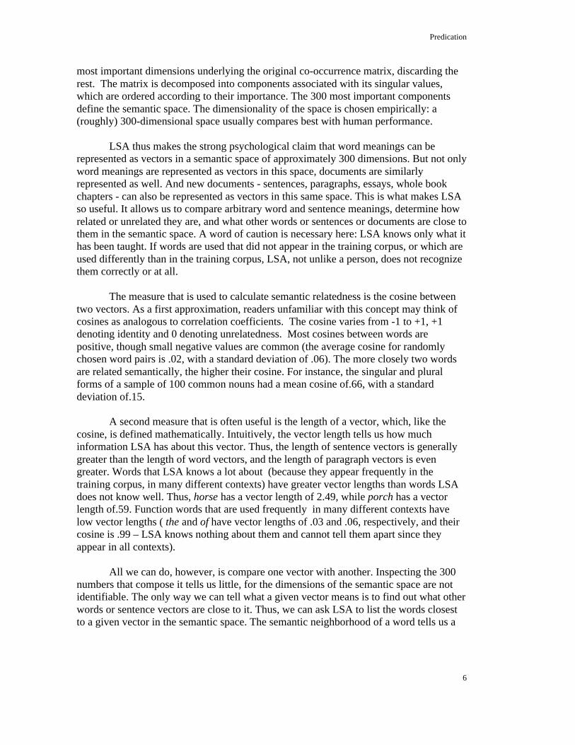
The measure that is used to calculate semantic relatedness is the cosine betweentwo vectors. As a first approximation, readers unfamiliar with this concept may think ofcosines as analogous to correlation coefficients. The cosine varies from -1 to +1, +1denoting identity and 0 denoting unrelatedness. Most cosines between words arepositive, though small negative values are common (the average cosine for randomlychosen word pairs is .02, with a standard deviation of .06). The more closely two wordsare related semantically, the higher their cosine. For instance, the singular and pluralforms of a sample of 100 common nouns had a mean cosine of.66, with a standarddeviation of.15.

A second measure that is often useful is the length of a vector, which, like thecosine, is defined mathematically. Intuitively, the vector length tells us how muchinformation LSA has about this vector. Thus, the length of sentence vectors is generallygreater than the length of word vectors, and the length of paragraph vectors is evengreater. Words that LSA knows a lot about (because they appear frequently in thetraining corpus, in many different contexts) have greater vector lengths than words LSAdoes not know well. Thus, horse has a vector length of 2.49, while porch has a vectorlength of.59. Function words that are used frequently in many different contexts havelow vector lengths ( the and of have vector lengths of .03 and .06, respectively, and theircosine is .99 – LSA knows nothing about them and cannot tell them apart since theyappear in all contexts).

All we can do, however, is compare one vector with another. Inspecting the 300numbers that compose it tells us little, for the dimensions of the semantic space are notidentifiable. The only way we can tell what a given vector means is to find out what otherwords or sentence vectors are close to it. Thus, we can ask LSA to list the words closestto a given vector in the semantic space. The semantic neighborhood of a word tells us a

Predication

7

great deal about the word. Indeed, we shall make considerable use of semanticneighborhoods below.

Often we have some specific expectations about how a vector should be related toparticular words or phrases. In such cases it is most informative to compute the cosinebetween the vector in question and the semantic landmark we have in mind. In most ofthe examples discussed below when we need to determine what a vector that has beencomputed really means, it will be compared to such landmarks. Suppose we compute thevectors for horse and porch. To test whether what has been computed is sensible or not,we might compare these vectors to landmarks for which we have clear-cut expectations.For instance, the word gallop should have higher cosine with horse than with porch(the cosines in fact are .75. and .10, respectively), but the word house should have ahigher cosine with porch than with horse (the cosines are .08 for horse and .65 forporch). This is not a very powerful test, but it is intuitively compelling and simple. Whatthe particular landmarks are is not terribly important, as long as we have clear sharedsemantic expectations. Someone else might have chosen race instead of gallop, or doorinstead of house, or many other similar word pairs, with qualitatively equivalent results.

Readers can make their own computations, or check the ones reported here, byusing the web site of the Colorado LSA Research group: http://lsa.colorado.edu. Firstselect the appropriate semantic space and dimensionality. The semantic space used hereis the "General Reading through First Year of College" space with 300 dimensions andterm-to-term comparisons. To find the semantic neighborhood of horse, one types"horse" into the Nearest-Neighbor-box and chooses “pseudodoc”. To find the cosinebetween horse and gallop, one types "horse" and into one box and "gallop" into the otherbox of the One-to-Many-Comparison.

LSA has proved to be a powerful tool for the simulation of psycholinguisticphenomena as well as in a number of applications that depend on an effectiverepresentation of verbal meaning. Among the former are Landauer and Dumais (1997),who have discussed vocabulary acquisition as the construction of a semantic space,modeled by LSA; Laham’s (1997) investigation of the emergence of natural categoriesfrom the LSA space; and Foltz, Kintsch, & Landauer’s (1998) work on textualcoherence. To mention just three of the practical applications, there is first, the use ofLSA to select instructional texts that are appropriate to a student's level of backgroundknowledge (Wolfe, Schreiner, Rehder, Laham, Foltz, Landauer, & Kintsch, 1998).Second, LSA has been used to provide feedback about their writing to 6th-grade studentssummarizing science or social science texts (E. Kintsch , Steinhart, Stahl, Matthews,Lamb, and the LSA Research Group, in press). The application of LSA that has arousedthe greatest interest is the use of LSA for essay grading. LSA grades the content ofcertain types of essays as well and as reliably as human professionals (Landauer, Laham,Rehder, & Schreiner, 1997). The human-like performance of LSA in these areas stronglysuggests that the way meaning is represented in LSA is closely related to the way humansoperate. The present paper describes an LSA-based computational model, whichaccounts for another aspect of language use, namely, how meaning can be modifiedcontextually in predication. The model is discussed first and illustrated with some simple

Predication

8

examples of predication. Then the model is used to simulate several more complex kindsof language processing.

LSA-Semantics: Predication

A semantic theory requires a definition of both the elements of the theory and therules for combining these elements. The elements of an LSA-semantics are the wordvectors in the semantic space. The standard composition rule for vectors in LSA has beento combine vectors by computing their centroid. Consider propositions of the formPREDICATE[ARGUMENT], where A is the vector corresponding to ARGUMENT andP is the vector corresponding to PREDICATE. According to the standard LSA practice,the meaning of the proposition is given by the centroid of A and P. In n dimensions, if A= {a1, a2, a3,.....an} and P = {p1, p2, p3,.......pn}, the centroid (A,P) = {a1+p1, a2+p2, a3+p3,........an+pn}. This is unsatisfactory, because the vector P is fixed and does not depend onthe argument A, in contradiction to the argument above that P means something different,depending on the argument it takes. Every time we use P in a different context A, we donot predicate all of P about A, but only a subset of properties of P that are contextuallyappropriate for A. This subset may be quite unusual and specific to that context (as insome of the examples above) or it may be large and diffuse, in which case the centroidmay provide an adequate description of the meaning of the whole proposition.

To capture this context dependency an alternative composition rule, thepredication algorithm, is proposed here. The essential characteristic of this algorithm isto strengthen features of the predicate that are appropriate for the argument of thepredication. This is achieved by combining LSA with the construction-integration modelof text comprehension (Kintsch, 1988, 1998). Specifically, items of the semanticneighborhood of a predicate that are relevant to an argument are combined with thepredicate vector, in proportion to their relevance through a spreading activation process.

The 300 numerical values of a word vector define the meaning of a word in LSA.This is a context-free definition, or rather, meaning is defined with respect to the wholetraining corpus. Another way of representing aspects of the meaning of a word is bylooking at its neighbors in the semantic space. The closest 20 or 100 neighbors tell ussomething about the meaning of a word, though not as much as the vector itself, whichpositions the word in the semantic space with respect to all other words. The closestneighbors, however, index some important features of the word and contexts in which itis used.

Consider a proposition of the form P(A), where P and A are terms in the LSAsemantic space represented by vectors. In order to compute the vector for P(A), theconstruction-integration model of Kintsch (1988,1998) will be used. Let {S} be the setof all items in the semantic space except for P and A. The terms I in {S} can be arrangedin a semantic neighborhood around P: their relatedness to P (the cosine between eachitem and P) determines how close or far a neighbor they are. Almost all items in the spacewill be at the periphery of the neighborhood, with cosines close to 0, but some items will

Predication

9

cluster more or less densely around P. Let cos(P, I) be the cosine between P and I in {S}.Furthermore, let cos(A, I) be the cosine between A and item I in {S}.

A network consisting of the nodes P, A, and all I in {S} can be constructed. Oneset of links connects A with all other nodes. The strength s(A,I) of these links iscodetermined by how closely related they are to both A and P:

s(A,I) = f(cos(A,I), cos(P,I))The function f must be chosen in such a way that s(A,I) > 0 only if I is close to both Pand A. A second set of links connects all items I in {S} with each other. These links havelow negative strengths, that is, all items I interfere with each other and compete foractivation. In such a self-inhibiting network, the items most strongly related to A and Pwill acquire positive activation values, whereas most items in the network will bedeactivated because they are not related to both A and P. Thus, the most stronglyactivated nodes in this network will be items from the neighborhood of P that are in someway related to A.

The k most strongly activated items in this network will be used in theconstruction of the vector for P(A). Specifically, the vector computed by the predicationprocedure is the weighted average of the k most activated items in the net describedabove, including P and A, where the weights are the final activation values of the nodes.

An example will help to clarify how this predication algorithm works. Considerthe sentences The horse ran, which has the predicate ran and the argument horse (Figure1). In predication, we first compute the neighborhood of the predicate ran – a set of itemsordered by how strongly related they are to ran. For the sake of simplicity, only threeitems from the neighborhood of ran are shown in Figure 1: stopped, down, and hopped,which have cosines with ran of .69, .60, and .60, respectively. A network is constructedcontaining these three items, the predicate ran and the argument horse, as shown inFigure 1. The neighbors are connected to ran with links whose strength equals the cosinebetween each neighbor and ran. Next, the cosines between the neighbors and thearguments horse are computed (which equal .21, .18, and .12, respectively) and thecorresponding links are added in Figure 1. We also add a link between ran and horse,with a strength value equal to the cosine between them (.21). Finally, inhibitory links areinserted between each pair of neighbor-nodes. Activation is then spread in this network(using the CI program described in Kintsch, 1998), until a steady state is reached. Thisintegration process will select items that are close to ran, but also relevant to horse: inthis case, ran and stopped will be most strongly activated, down will be somewhatactivated, and hopped will receive no activation.

Figure 1

In the computations below two approximations are used:(1) First, instead of constructing a huge network comprising all items in the

semantic space, almost all of which would be rejected anyway, only the m closestneighbors of a predicate will be considered. The size of m varies because in order toselect the terms that are most relevant to both A and P, a smaller or larger neighborhoodmust be searched, depending on how closely related A and P are. Thus, for most

Predication

10

sentences combining familiar terms in expected ways, m = 20 works well, because termsrelated to A will be found even among the closest neighbors of P. For metaphors, on theother hand, where the predicate and argument can be quite distant, the crucial terms areusually not found among the top 100 neighbors of the predicate, and m needs to belarger, say 500 neighbors. A neighborhood of 1500, on the other hand, is too large: theterms selected from such a large neighborhood by the predication algorithm may onlyhave a tenuous relationship to P and hence misrepresent it.

(2) Instead of using a weighted average of P and the k most relevant neighbors forthe vector representing P(A), the weights will be neglected. Since only small values of kare used and the differences in activation among the top few terms are usually notdramatic, this computational shortcut has little effect. It greatly simplifies the calculationof predicate vectors, however. Since the most highly activated terms in the neighborhoodof a predicate are those with the highest cosine to the argument, one merely has to add thek top-ranked terms to A and P. Thus, the vector for P(A) is computed as the centroid ofP, A, and the k most activated neighbors of P (normally, LSA represents the meaning ofP(A) simply as the centroid of P and A; the predication algorithm biases this vector byincluding k contextually appropriate neighbors of P).

The parameter k must neither be too small nor too large. If too few terms areselected, a relevant feature might be missed; if too many terms are selected, irrelevantfeatures will be introduced. Values between k = 1 and k = 5 have been found to be mostappropriate. When processing is more superficial, as in the similarity judgmentsdiscussed below, k = 1 gives the best results. If deeper understanding is required, k -values of 3 or 5 appear optimal. Selecting more than 5 terms usually introduces unwantednoise.

Some Simple Examples of Predication

How satisfactory is the proposed predication algorithm? It is difficult to give astrong answer to this question. If there existed a closed set of sentences corresponding toP(A) propositions, one could obtain a random sample, compute the correspondingvectors, and find some way to compare the result with our intuitions about the meaning ofthese sentences. Instead, all that can be done is to show for a few simple samplesentences that the predication algorithm yields intuitively sensible results, and then focuson some semantic problems that provide a more demanding test. Metaphor interpretation,causal inferences, similarity judgments, and homonym disambiguation are somedomainsthat allow a more specific evaluation as well as some comparisons between setsof experimental data and LSA predictions.

As an example of simple predication, consider the vectors corresponding to Thehorse ran and The color ran. First, the closest 20 neighbors to ran in the LSA space arecomputed. This list includes ran itself, since a word is always part of its ownneighborhood. Then, the cosines between these 20 terms and horse and color,respectively, are calculated. A net is constructed linking horse, respectively color, withthe 20 neighbors of ran, with link strength equal to the cosine between each pair of termsand inhibitory links between each of the 20 neighbors. The absolute value of the sum of

Predication

11

all negative links is set equal to the sum of all positive links, to insure the proper balancebetween facilitation and inhibition in the network. This network is then integrated,resulting in final activation values for each of the 20 neighbors. These calculations aresummarized in Table 1.

Table 1

The vector for The horse ran computed by predication is therefore the centroid ofhorse, ran, and the 5 most highly activated terms from the neighborhood of ran (column3 Table 1), which are ran itself and stopped, yell, came and saw. The vectorrepresenting the meaning of The color ran is obtained in the same way: it is centroid ofcolor, ran, and down, shouted, looked, rushed, and ran. Thus, while ran has differentsenses in these two contexts, these senses are by no means unrelated: ran in the color-sense is still strongly tied to movement verbs like rushed and hurry.

It is important to note that just which words are selected from a neighborhood bythe predication algorithm does not have to be intuitively obvious, and often is not (likethe choice of yell for the horse-sense of ran above): what needs to be intuitivelymeaningful is the end result of the algorithm, not the intermediate steps. In many cases,items from a neighborhood are selected that seem far from optimal to our intuitions; theyachieve their intended purpose because their vectors have weights on the abstract featuresthat are relevant in this particular context.

To interpret the meaning of these vectors, they are compared to appropriatelandmarks. Landmarks need to be chosen so as to highlight the intuitively importantfeatures of the sentence. Gallop was chosen as a landmark that should be closer to horseran than color ran, and dissolve (a synonym for this sense of run according to WordNet)was chosen to be closer to color ran than to horse ran. This is indeed the case, as shownin Table 2. Ran by itself is close to gallop, but is essentially unrelated to dissolve. Forhorse ran, the relationship to gallop is strengthened, but the relationship to dissolveremains the same. The opposite result is obtained when ran is put into the context color:the relationship to gallop is weakened (but it does not disappear – the color ran hasdifferent connotations than the color dissolved) and that to dissolve is strengthened .

Table 2

Choosing different landmarks, say race and smudges, yields a qualitativelysimilar picture. Varying the size of the semantic neighborhood (parameter m) has littleeffect in this example, either. For m = 50 and m = 100 the cosines with the landmarksvary by a few percentage points, but the qualitative picture remains unchanged.

The horse ran is a more frequent expression than The color ran. In fact, in thecorpus on which the semantic space used here is based, color ran appeared only once (inabout 11 million words), whereas horse ran was present 12 times in the input data. Thus,LSA had little occasion to learn the meaning of color ran. Most of the interpretation thatLSA gives to color ran is based on indirect evidence, rather than on direct learning.Indeed, if the semantic space is re-scaled with the single mention of color ran omitted,Table 2 remains basically unchanged. Thus, LSA can generate an intuitively plausible

Predication

12

interpretation for a word sense it has never experienced: it does not need to be trained onthe specific sense of ran in the context of color, it can generate the right meaning for thesentence on the basis of whatever else it knows about these words. As Landauer andDumais (1998) have argued, vocabulary acquisition does not consist in learning aboutmany thousands of separate word meanings, but in constructing a semantic space andembedding words and phrases into that space.

A second example of simple predication involving different senses of a word isshown in Figure 2 where the meanings of the sentences The bridge collapsed, The planscollapsed, and The runner collapsed are compared. The landmarks were chosen in such away that each sentence should be closest to one of the landmarks. The results confirmthese expectations. The landmark break down is closest to The bridge collapsed.Appropriately, plans collapsed is closest to failure. For the race landmark, runnercollapsed is closest. Thus, these results agree reasonably well with our intuitions aboutwhat these sentences mean. However, this is not the case when the sentence vectors arecomputed as simply the centroid of the subject and verb. In that case, for instance, breakdown is approximately equidistant to all three sentences.

Figure 2

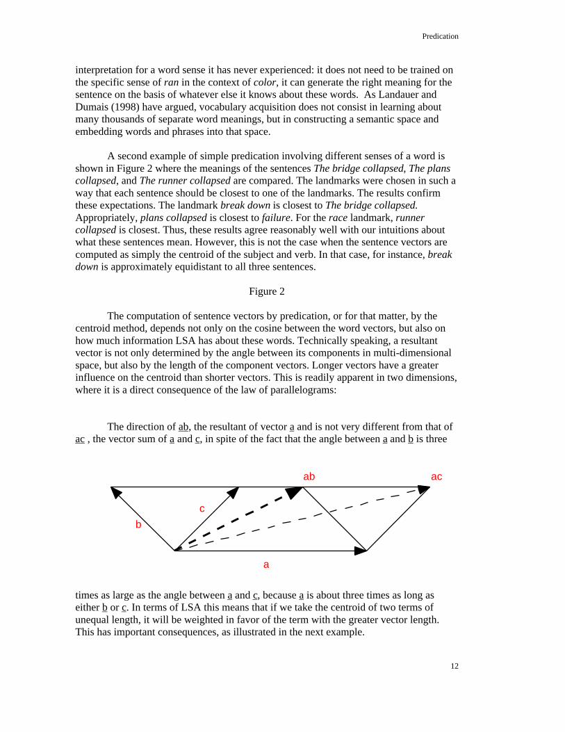
The computation of sentence vectors by predication, or for that matter, by thecentroid method, depends not only on the cosine between the word vectors, but also onhow much information LSA has about these words. Technically speaking, a resultantvector is not only determined by the angle between its components in multi-dimensionalspace, but also by the length of the component vectors. Longer vectors have a greaterinfluence on the centroid than shorter vectors. This is readily apparent in two dimensions,where it is a direct consequence of the law of parallelograms:

The direction of ab, the resultant of vector a and is not very different from that ofac , the vector sum of a and c, in spite of the fact that the angle between a and b is three

times as large as the angle between a and c, because a is about three times as long aseither b or c. In terms of LSA this means that if we take the centroid of two terms ofunequal length, it will be weighted in favor of the term with the greater vector length.This has important consequences, as illustrated in the next example.

a

b

c

acab

Predication

13

The vector for bird has length 2.04 while the vector for pelican has length 0.15,reflecting, in part, the fact that LSA knows a lot more about birds than about pelicans.When the two terms are combined, the longer vector completely dominates: the cosinesbetween bird+pelican and the individual terms bird and pelican are 1.00 and .68,respectively. For comparison, the cosine between bird and pelican is .64. In other words,pelican doesn't make a dent in bird.

That result has serious consequences for predication. Of course, the centroid doesnot distinguish at all between The bird is a pelican and A pelican is a bird. Predicationdoes, but with very asymmetric results. A pelican is a bird turns the pelican into a bird,almost totally robbing it of its individuality, as shown in Figure 3. Pelican is a birdbehaves like a bird with respect to the five landmarks in Figure 3 - closer to singsbeautifully than to eat fish and sea! If we combine a short and a long vector, we get backbasically the long vector - if the differences in vector length are as pronounced as in thecase of bird and pelican, which differ by a factor of 13.

Figure 3

Figure 4 illustrates what happens when the direction of predication is reversed.For LSA the meaning of A bird is a pelican is about the same as the meaning of bird byitself. Since LSA is vague about pelicans, we are not adding much meaning or knowledgeto bird by saying it is a pelican.

Figure 4

A distinction needs to be made here between knowledge and information. LSArepresents cumulative knowledge, not transient information. It measures not the newinformation provided by a sentence but what we already knew about its components.Predicating pelican about bird (The bird is a pelican) adds very little to our knowledgebecause we (and LSA) know very little about a pelican, other than that it is a kind of bird- it eats a little bit more fish than most birds do and sings a little bit less beautifully. Thevector for bird is pelican is not very different from the vector for bird. In contrast, thesentence The bird is a pelican conveys information, because it excludes numerous otherpossibilities. On the other hand, pelican is a bird modifies our knowledge of pelican byemphasizing its general bird-features and de-emphasizing its individuality as a pelican.The language marks these distinctions. We say The bird is a pelican, providinginformation about some specific bird. Or we say A pelican is a bird, referring to thegeneric pelican. In the first case, we provide information, in the latter we provideknowledge. The informationally empty The pelican is a bird, and the epistomologicallyempty A bird is a pelican are not common linguistic expressions.

A similar distinction can be made between information and knowledge in a text.For each text, there exists relevant background knowledge with respect to the topic of thetext. The text itself, however, usually involves information that is new and not alreadyrepresented in the background knowledge. Thus, in a story unexpected things are

Predication

14

supposed to happen, building upon but different from what we already know. Thetextbase represents this new information in a text, while LSA provides a representation ofthe relevant background knowledge - what we already knew before we read the text. Incomprehending the text, a representation is constructed – the situation model – thatintegrates the novel textual information and the pre-existing background knowledge.

Metaphors

As long as we are dealing with simple, familiar sentences, the results obtainedwith the predication algorithm often do not differ much from computations using thesimpler centroid method. We need to turn to semantically more demanding cases toappreciate the full power of predication. The first of these cases is metaphorcomprehension. This topic is discussed more fully in Kintsch (in press). It will be brieflysummarized here, because it is crucial for an understanding of predication.

Experimental psycholinguistic evidence implies that metaphoric predication isjust like any other predication in terms of the psychological processes involved (forreviews see Glucksberg & Keysar, 1994; Glucksberg, 1998; Gibbs, 1994). Thus, we needto show that applying the predication algorithm to metaphors in exactly the same way asit is applied to other sentences yields sensible interpretations of metaphors. Kintsch (inpress) did just that. It showed that the interpretations of metaphors arrived at by thepredication procedure agree with our intuitions reasonably well and, furthermore,demonstrated that some of the major phenomena in the experimental literature onmetaphor comprehension can be simulated in this way, as direct consequences of thepredication algorithm.

Figure 5

Glucksberg (1998) discusses in some detail the metaphor My lawyer is a shark.Figure 5 presents the results of a comparison of the vector for lawyer alone and the vectorcomputed by predication for My lawyer is a shark with landmarks chosen to highlightboth the relevant and irrelevant features of the metaphor. By itself, lawyer is stronglyrelated to concepts like justice and crime, not at all related to shark and fish, but lawyer ismoderately related to viciousness. Predicating shark about lawyer changes this pictureconsiderably. The lawyer-properties remain strong. The interesting thing is what happensto the shark-properties: viciousness is emphasized, in agreement with my intuitions thatMy lawyer is a shark means something like My lawyer is vicious. But it does not meanexactly that, otherwise we might have said so in the first place. There is also a little bit ofshark and fish in it, and if we look at bloodthirsty or tenacious, we would see thatelevated, too. Thus, the meaning of a metaphor is not fully captured by a literalparaphrase, but is richer, more expressive, and fuzzier than corresponding literalexpressions.

Figure 5 totally depends on the use of the predication algorithm. If the meaning ofthe metaphor is computed as the centroid of the words, the results do not make sense. Thecentroid of lawyer and shark is somewhere in semantic no man’s land: more strongly

Predication

15

related to shark and fish (cosines of .83 and .58, respectively) than to any of the lawyer-properties or to viciousness.

To compute the predication vector in Figure 5 a semantic neighborhood of m =500 was used. When a predicate and argument are semantically related, features that arerelevant to both can usually be found even with lower values of m. Thus, for thecalculations in the previous section m was typically set to equal 20. For metaphors,where argument and predicate can be quite unrelated in their literal senses, as in thepresent example, a larger semantic neighborhood must be searched to find three or fiveterms relevant to the predication. Furthermore, in order to insure that all terms selectedare at least minimally related to both P and A, a threshold of two standard deviationsabove the mean for all words in the space was used. Since the mean cosine between allword pairs in the space is .02 and the standard deviation is .06, this meant that all cosineshad to be at least .14. For m < 100, predication fails (the concept lawyer is not modifiedat all – there are no terms among the 100 closest LSA neighbors of shark that aresemantically related to lawyer, that is, terms whose cosine with lawyer is at least .14, thethreshold value we have chosen). For m = 500, 1000 or 1250, roughly equivalent resultsare achieved. As the neighborhood grows too large (m = 1500) the procedure begins topick up random noise.

One of the salient facts about metaphors is that they are, in general not reversible.Reversed metaphors either mean something different, or they do not mean much at all.Kintsch (in press) has shown that the predication algorithm yields results in agreementwith these intuitions. Surgeon is related semantically to scalpel, but not to axe; thereverse is true for butcher. My surgeon is a butcher has a cosine of .10 with scalpel and acosine of .42 with axe; the reversed metaphor, My butcher is a surgeon has a cosine of.25 with scalpel and .26 with axe. On the other hand, reversing My shark is a lawyerdoes not yield any clear interpretation at all.

In order to assess the generality of the predication algorithm, Kintsch (in press)analyzed the first seven examples of nominal metaphors cited in Glucksberg, Gildea &Bookin (1982). Overall, the algorithm produced satisfactory results: the cosine betweenthe metaphor and the relevant landmark was significantly higher than between themetaphor and the irrelevant (literal) landmark. The analysis failed in the case of Hermarriage is an icebox – apparently because the LSA space used did not know enoughabout iceboxes, nor about cold marriages. This failure illustrates the need to distinguishbetween the adequacy of the underlying knowledge space and the predication algorithmitself. If LSA does not know something, it will perform badly with any algorithm;however, all one would presumably have to do in this case is to train LSA with a richerand more informative body of texts.

Two interesting phenomena about the time course of metaphor comprehension arealso discussed in Kintsch (in press). First, it has been shown (Glucksberg, McGlone, &Manfredini, 1997) that the time it takes to comprehend a metaphor is increased when theliteral meaning is primed. Thus, after reading sharks can swim, My lawyer is a sharkrequires more time to comprehend than after a neutral prime. The literal prime activates

Predication

16

those features of shark that are related to swim. Hence, in the CI model, when themetaphoric sentence is being processed, the wrong features start out with a highactivation value and it takes several integration cycles to deactivate the literal featuresand activate the metaphoric features. As the reverse of that, a metaphoric prime can slowdown the comprehension of a literal sentence (Gernsbacher, Keysar, & Robertson, 1995).If My lawyer is a shark precedes sharks can swim in a sentence verification task,verification times are longer than if a neutral prime is used. The account that thepredication model gives is essentially the same as in the first case. The metaphoractivates features like viciousness and deactivates features like fish, so when sharks canswim must be verified, the wrong features are active and it requires several cycles of theintegration process to deactivate these features and at the same time boost the activationof the features that are relevant to swim.

Thus, Kintsch (in press) goes beyond demonstrating that the predication modelyields intuitively sensible interpretations of metaphors. It also shows that some of themajor phenomena about metaphor comprehension in the psycholinguistic literature arereadily accounted for within that framework. This is of interest, on the one hand, becauseit suggests that metaphor comprehension can indeed be treated in the same way as literalpredication, and on the other hand, because it provides a good demonstration of how thepredication algorithm extends the range of phenomena that LSA can account for.

Causal Inferences

Many sentences imply causal consequences or causal preconditions. Thus, Thedoctor drank the water implies pragmatically (though not logically) the causalprecondition that the doctor was thirsty, and The student washed the table implies thecausal consequence that the table was clean. Usually, these are described as causalinferences, though some authors, such as Kintsch (1998), argue that the term inference ismisleading in this context. When we read The student washed the table we do notusually, in addition, draw an inference that the table is clean. Rather, comprehending thatsentence automatically makes available this information, without any extra processing.Long-term working memory assures that there will be a link between the sentence Thestudent washed the table and its anticipated causal consequence, the table was clean.LSA provides a computational model of how long-term working memory functions incases like these. Kintsch, Patel, & Ericsson (1999) have argued that the semantic spacefunctions as the retrieval mechanism for working memory. Thus, if understanding Thestudent washed the table involves computing its vector in the semantic space, closelyrelated vectors such as The table was clean automatically become available in long-termworking memory and may be subject to further processing (e.g., in a sentence verificationtask).

It remains to show that predication indeed delivers the right kind of results. Aresentence vectors in LSA, computed by predication, closer to causally related inferencesthan to causally unrelated but superficially similar sentences? Specifically, is the vectorfor The student washed the table closer to The table was clean than to The student wasclean?

Predication

17

We are concerned with subject-verb-object sentences, that is, propositions of theform

PREDICATE[ARGUMENT1<AGENT>, ARGUMENT2<OBJECT>].The corresponding syntactic structure is given by

NP(N1)+VP(V+N2).The syntax suggests that propositions of this form involve two separate predicationoperations: first V is predicated about N2, in the same way as discussed for simplepredication above; then VP is predicated about N1.

Specifically, in Step 1 the neighborhood of size m (m = 20) for the predicate V isobtained. We select those terms from this neighborhood that are most relevant to N2: anetwork consisting of N2 and all neighbors, with link strengths equal to the cosinebetween N2 and each neighbor, is integrated and the k (k = 5) terms with the highestactivation values are used to approximate the vector for (V+N2). In Step 2 theneighborhood is calculated for the complex predicate (V+N2), consisting of V, N2 andthe k most relevant neighbors selected in Step 1. N1 is then used to determine therelevant terms from that neighborhood. The sentence vector, then, is approximated by thecentroid of N1, V, N2, the k neighbors selected in Step 1, and the k neighbors selected inStep 2.

Thus, LSA, guided by a syntactic parse of the sentence, constructs a vector thatrepresents the meaning of the proposition as a whole. To evaluate how well a predicationvector captures the intuitive meaning of a proposition, causal inferences will be chosen aslandmarks. For example,

The student washed the table --consequence--> the table is cleanor

The doctor drank the water --precondition--> the doctor was thirsty.The vector representing the meaning of the sentence The student washed the table,computed by the predication procedure outlined above should be closer to the correctinference the table is clean than to the incorrect inference the student is clean.

As Table 3 shows, this is not generally the case when the meaning of the sentenceis represented by the centroid of the three words. In fact, for the four examples analyzedhere, the centroid makes the wrong inference in three cases. As we have seen above, thecentroid is heavily influenced by vector length, so that semantically rich terms, likehunter, will always dominate semantically sparse terms, like elk. The predicationprocedure is able to overcome this bias in three of the four cases analyzed here. Forinstance, the doctor drank the water is strongly biased towards the water was thirsty, butpredication manages to reverse that bias. Similarly for

The student washed the table --> the table was clean,The student dropped the glass --> the glass was broken.

However, the wrong conclusion is reached in the case ofThe hunter shot the elk --> the hunter was dead.

But even where predication fails to detect the correct inference, the cosine for the elk wasdead increased twice as much as the cosine for the hunter was dead as a result of

Predication

18

predication over a centroid based comparison. Apparently predication does somethingright, but may have failed for parametric reasons.

Table 3

There are two parameters that need to be explored: the size of a predicateneighborhood was set at m = 20, and the number of most relevant terms chosen torepresent the predicate vector was set at k = 5. Exploratory calculations suggest that thesechoices of parameter values are not necessarily optimal.

The calculations for The hunter shot the elk were repeated with the size of thepredicate neighborhood m = 100. Increasing the neighborhood size, however, did notimprove the performance of LSA in this case. Indeed, the bias in favor of hunter deadwas slightly increased: the cosine between the sentence vector computed with m = 100and hunter dead turned out to be .77, versus .72 for elk dead. What seemed to happenwas that as the number of possible selections increased, the argument could select termsit liked that were, however, too distant from the predicate. For instance, when theneighborhood of elk shot is so large, rather distant terms like bow and arrow can beselected because they are so close to hunter, biasing the meaning of the sentence ininappropriate ways.

Better results were obtained by manipulating k, the number of terms used toapproximate the predication vector. A smaller value of k than 5 which was used so farmight work better, because in some cases the first three or four words that were selectedfrom a neighborhood appeared to make more sense intuitively than the last ones. Hencethe computations for The hunter shot the elk were repeated with k = 3. This resulted insome improvement, but not enough: the cosine between The hunter shot the elk andhunter dead became .69, versus .68 for elk dead.

Another possibility is that LSA just does not know enough about elks. If the morefamiliar word deer is substituted for elk, things improve. For k = 3, we finally get

The hunter shot the deer --> the deer is dead.The cosine between The hunter shot the deer and The deer is dead is .75, whereas thecosine with The hunter is dead is now only .69.

An application of the predication algorithm to an existing set of examples ofcausally linked sentences uses materials developed by Singer, Halldorson, Lear, &Andrusiak (1992). In this well-known study, Singer et al. (1992) provided evidence thatcausal bridging inferences were made during reading. In Experiment IV, sentence pairs inwhich the second sentence states a causal consequence of the first were compared withsentence pairs in which the second sentence merely follows the first temporally. Anexample of a causal sentence pair would be Sarah took the aspirin. The pain went away.An example of temporal succession would be Sarah found the aspirin. The pain wentaway. Their stimulus materials provide a further test of the ability of the predicationmodel to explain causal inferences: the semantic relatedness between the sentencesshould be greater for the first than for the second pair of sentences.2 Five of their stimuli

Predication

19

were of the simple S-V-O form (or could be rewritten in that form with slight, inessentialmodifications) required by the present analysis; the other examples were syntacticallymore complex. The following sentence pairs could be analyzed:

Sarah took/found the aspirin. The pain went away.(.89/.47)Harry exploded/inflated the paper bag. He jumped in alarm.(.33/.28)The hiker shot/aimed-at the deer. The deer died. (.74/.56)Ted scrubbed/found the pot. The pot shone brightly.(.45/.41)The camper lost/dropped a knife. The camper was sad.(.48/.37)

The numbers in parentheses below each line show the cosine values that were computedbetween the first and second sentence. 3 In every case, causally related sentences had ahigher cosine than temporally related sentences. The average cosine for causally relatedsentence pairs was .58, versus .42 for temporally related sentence pairs.

Together with the examples presented in Table 3, the analysis of the stimulusmaterials from Singer et al. (1992) suggests that predication can give a satisfactoryaccount of causal inferences in comprehension. Causally related sentence pairs appear tohave generally higher cosines than appropriate control items, showing that the model issensitive to the causal relation; the model does not yet tell us, however, that what it hasfound is a causal relation.

Judgments of Similarity

Another domain where the predication model will be applied is that of similarityjudgments. The cosines between concepts computed by LSA do not correlate highly withsimilarity judgments. Mervis, Rips, Rosch, Shoben, & Smith(1975; reprinted in Tversky& Hutchinson, 1986) reports similarity judgments for a 20 x 20 matrix of fruit names.The correlation between these judgments and the cosines computed from LSA isstatistically significant, but low, r = .32. Similarly, for the data reported below in Table4, the correlation between similarity judgments and the corresponding cosines is r = .33.These results appear to be representative.4 In fact, there is no reason to believe that thesecorrelations should be higher. It has been generally recognized for some time now thatsimilarity judgments do not directly reflect basic semantic relationships but are subject totask- and context-dependent influences. Each similarity judgment task needs to bemodeled separately, taking into account its particular features and context.

It makes a difference how a comparison is made, what is the predicate and what isthe argument. Tversky and Hutchinson (1986) point out that we say Korea is like China,but not China is like Korea, presumably because the latter is not very informative andthus violates Gricean maxims. The predication model provides an account for thisobservation. In Korea is like China, Korea is the argument and China the predicate; thusthe resulting vector will be made up of Korea plus China-as-relevant-to-Korea - just as A

Predication

20

pelican is a bird was made up of pelican plus bird-as-relevant-to-pelican. (Obviously, isand is-like do not mean the same, but this by no means irrelevant distinction must beneglected here). On the other hand, for China is like Korea, we compute a vectorcomposed of China and Korea-as-relevant-to-China. The results are quite different. Tosay China is like Korea is, indeed, much like saying Bird is pelican - both statements aresemantically uninformative! The cosine between China and Korea-as-relevant-to-Chinais .98, that is we are saying very little new when we predicate Korea about China in termsof the LSA semantics of the two concepts. However, to say Korea is like China, yields acosine of only .77 between Korea and China-as-relevant-to-Korea. Our rich informationabout China modifies our concept of Korea successfully, whereas the little we knowabout Korea is so much like China anyway that it has not much of an impact on ourconcept of China.

The reason for the asymmetry in the previous example lies in the difference in theamount of knowledge LSA has about China and Korea: the vector length for the formeris 3.22, versus 0.90 for the latter. When the vector length of the words being compared ismore equal, the order of comparison may not make much of a difference. Thus, forButtons are like pennies and Pennies are like buttons, the cosine between buttons andpennies-like-buttons is .32, which is about the same, .28, as the cosine between penniesand buttons-like-pennies. Even if there are differences in vector length when the wordsbeing compared are basically unrelated, order differences may be minor. For Buttons arelike credit cards and Credit cards are like buttons, roughly equal cosines are obtained forthe two comparisons (.04 and .07, respectively), in spite of the fact that credit cards has avector length of 3.92, ten times as much as buttons.

The literature on similarity judgments is huge and complex and it is not at allclear at this point just which phenomena the predication model can account for and whatits limits are. However, one systematic comparison with a small but interesting data setwill be described here. Heit and Rubenstein (1994) report average similarity judgmentsfor 21 comparisons with two different instructions. In one case, subjects were told tojudge the similarity between a pair of animal names focusing on "anatomical andbiological characteristics, such as internal organs, bones, genetics, and body chemistry".In another conditions, subjects were asked to focus on "behavioral characteristics, such asmovement, eating habits, and food-gathering and hunting techniques" (p. 418). Theseinstructions made a great deal of difference. For instance, hawk-tiger was judged highlysimilar with respect to behavior (5.72 on a 10-point scale) but not with respect toanatomy (2.29), whereas shark-goldfish were more similar with respect to anatomy (5.75)than with respect to behavior (3.60). Intuitively, one would expect such results - thequestion is whether LSA has the same intuitions or not.

In terms of the predication model, either Anatomy or Behavior were predicatedabout each animal name to be judged. What was compared was Animal1-with-respect-to-behavior and Animal2-with-respect-to-behavior on the one hand, and Animal1-with-respect-to-anatomy and Animal2-with-respect-to-anatomy on the other. Specifically, thesemantic neighborhoods of both instruction sentences quoted above were determined, andthe terms most relevant to the to-be-compared words were selected and combined with

Predication

21

the word vector. Table 4 shows that LSA predicted the results of Heit and Rubensteinvery well indeed. There are eight comparisons (rows 1-8 in Table 4) for whichanatomical similarity was greater by at least one point than behavioral similarity. Forthese comparisons the cosines for the with-respect-to-anatomy comparisons were greater(equal in one case) than those for the behavioral comparison. There were four word pairsfor which the behavioral similarity was rated at least one point higher than the anatomicalsimilarity (rows 18-21). In all these cases the cosines for the behavioral comparisonswere higher than for the anatomical comparisons. On the other hand, for the nine wordpairs for which the empirical results were inconclusive (average ratings differed less thanone point, rows 9-17), LSA matched the direction of the difference only in 4 cases.Average results are shown in Figures 6, where the difference between Behavior minusAnatomy for the rating data as well as the cosines is plotted for items rated more similarin terms of behavior, neutral items, and items rated more similar in terms of anatomy.

Table 4, Figure 6

The predictions reported here are based on computations using a semanticneighborhood of size m = 50 and a selection of one term from that neighborhood to becombined with the vector for each word (k = 1). Larger values of k yielded somewhatless satisfactory predictions. The correlation between the rating differences Anatomy-Behavior and the corresponding cosine difference were r = .62, r = .51, and r = .40 for k =1, 3, or 5, respectively. Calculations based on a semantic neighborhood of m = 20,however, produced poor results. Only in very few cases could something relevant to theanimal names be found in the anatomy neighborhood when only 20 terms were used.Thus, for this choice of parameter value behavior almost completely dominated anatomy,since even in a small neighborhood of behavior terms like eating were to be found, i.e.,terms that are more or less relevant to all animals.

To account for the Heit & Rubenstein data, the predication model was needed;simply computing the cosine between two terms misses the context dependency of thesejudgments. However, similarity judgments are not always context dependent. Acounterexample is given by Landauer & Dumais (1997), who were able to describe thechoices people make on the TOEFL test (Test of English as a Foreign Language) simplyby computing the cosine between the word to be judged and the alternatives amongwhich a choice had to be made. For instance, what is the right response for the test wordabandoned – forsake, aberration, or deviance? The cosines between the test word andthe alternatives are .20, .09, and .09, respectively, so LSA chooses the right response.Indeed, LSA chooses the correct alternative 64% of the time, matching the mean percentcorrect choices of foreign students who are taking this test. It is easy to see why LSAalone works so well here, but why it must be used in conjunction with the predicationalgorithm for the Heit & Rubenstein data. The multiple choice alternatives on theTOEFL test do not provide a meaningful context with respect to which similarity can bejudged because they are unrelated words (in the present example, the average cosineamong the alternatives is .07), whereas in the examples discussed above, context plays adecisive role.

Predication

22

Homonyms

Predication modifies the predicate of a proposition in the context of itsargument(s). However, the arguments themselves may have multiple senses or, indeed,multiple meanings. Homonyms are words that are spelled the same but have severaldistinct meanings – not just different senses. The vector that LSA computes for ahomonym lies near both of its distinct meanings, something that is quite possible in ahigh-dimensional space. An example from Landauer (in preparation) will illustrate thispoint. Take the word lead. Its cosine with metal is .34 and its cosine with follow is .36;however, the cosine between metal and follow is only .06. Lead is related to twoneighborhoods that are not related to each other. The average cosine between lead and<metal, zinc, tin, solder, pipe> on the one hand and <follow, pull, direct, guide, harness>is .48. But the average cosine between the words in these two distinct neighborhoods is.06.

If a homonym is used as an argument in one of its meanings in a sentence, do weneed to adjust its meaning contextually similarly to the way it was done for predicates?Or does the predication procedure, which combines the vectors for the predicate andargument, automaticallyaaccomplish the meaning selection for arguments with multipleunrelated meanings? The latter appears to be the case. The LSA vectors forhomonymous nouns contain all possible meanings (with biases for the more frequentones), and appropriate predicates select fitting meanings from this complex. Someexamples will illustrate this claim.

Figure 7

According to WordNet, mint has four meanings as a noun, one as a verb, and oneas an adjective. Figure 7 compares three of these senses with suitable landmarks. Thesentences use the candy sense, the plant sense, and the verb sense of the homonym. Thevector for mint is roughly equally related to the three landmarks that capture the differentmeanings of the homonym, with a slight bias in favor of the candy meaning. Vectors forthese sentences were computed according to the predication procedure, and these vectorswere compared with landmarks emphasizing one of these meanings: chocolate for thecandy sense, stem for the plant sense, and money for the verb sense. Of course, once anargument is embedded in its sentence context, it is not possible to extract a separatevector for the argument; rather, the resulting vector represents the whole sentence.Figure 7 shows that these sentence vectors have become very specific: they are stronglyrelated to the appropriate landmarks, but only a little or not at all related to theinappropriate landmarks. However, the vectors for all three sentences remains related tothe word mint. That is, mint still plays an important role in the sentence, not just the othertwo context words (cosines between mint and the three sentences are .40, .27, and .38,respectively, for the candy, plant and coins sentence).

The mint-example comes, in somewhat different form, from a priming experimentby Till, Mross, & Kintsch (1988), where it was the first item in their list of experimentalmaterials. We also analyzed the next five of their examples with the predicationprocedure. For each homonym noun, two different disambiguating phrases were

Predication

23

constructed, using as predicates words from the definitions given in WordNet. Thus, forthe homonym pupil, the phrases used were pupil in school and pupil of the eye. Thesebrief contexts were clearly sufficient to determine the meaning of the homonym foreducated adults. Would they suffice also for LSA? For each phrase a vector wascomputed with the predication procedure as explained above (m = 50, k = 3). This vectorwas then compared to landmarks also selected from WordNet – the category names towhich each meaning was assigned in WordNet5. The following test list of homonyms andlandmarks was thus obtained: ball/game-shot; bit/stable gear-pieces; pupil/learner-opening; dates/day-fruit; foil/sheet-sword. Thus, 10 comparisons could be made. In 9cases, the cosine between the phrase vector and the appropriate landmark was higher thanthe cosine between the phrase and the inappropriate landmark. The average cosine valuefor appropriate landmarks was .37, compared with .16 for inappropriate landmarks. Theone failure that was observed was for the phrase fencing foil – the General Reading Spacedoes not know the fencing meaning of foil (the two words have a cosine of -.04). Notethat this indicates a lack of knowledge – not necessarily a failure of the predicationalgorithm.

Thus, it appears that the predication procedure is sufficient to contextualizewords that have different meanings, in the same way as it handles words that havedifferent senses. At least that is a reasonable hypothesis, pending further research.Gentner and France (1988) performed a series of experiments to investigate thecomprehension of sentences in which the noun and verb were mismatched to make theinterpretation of the sentence difficult. They concluded that under these conditions”verbs adjust to the nouns rather than the other way around.” Their results provide somesupport for the kind of model considered here.

Discussion

LSA-Semantics. LSA is a new theory of word meaning. It is a theory that hasconsiderable advantages over other approaches to lexical semantics, starting with the factthat it is a completely explicit mathematical formalism that does not depend on humanintervention. It has also been strikingly successful in practical applications and hasprovided a solution to one of the toughest previously unresolved puzzles in thepsychology of language - to explain the astonishing rate of vocabulary acquisition inchildren (Landauer & Dumais, 1997). Nevertheless, not everyone has been willing to takeLSA seriously as the basis for a semantic theory. Too many of the traditional concerns ofsemantics have been outside the scope of LSA. The predication algorithm that isproposed in the present paper rectifies this situation to some extent. By combining LSAwith the construction-integration model LSA can be made to account for the way inwhich syntax modifies meaning, at least for some simple, basic cases. At this point, it isnot clear where the limits of the predication model are in this respect. However, even ifthe proposed approach eventually yields a full and satisfactory account of predication,other fundamental semantic problems remain for LSA, for example, concerning theclassification and distinction among such semantic relations as hypernymy andhyponymy, meronymy, antonymy and so on.

Predication

24

Even though LSA is still only incomplete as a semantic theory, it neverthelessprovides an interesting and promising alternative to the dominant conceptions of lexicalsemantics. Providing a computational model of how the syntactic and semantic contextcan modify and shape word meanings makes it possible to think about a lexicon in whichword senses do not have to be distinguished. Words in LSA are represented by a singlevector in a high-dimensional semantic space, however many meanings or senses theymight have. The separate meanings and senses emerge as a result of processing a word inits syntactic and semantic context. They are therefore infinitely sensitive to the nuancesof that context - unlike predetermined definitions, that will never quite do justice to thedemands of complex linguistic contexts. Kintsch (1988, 1998) has argued that such atheory is required for discourse understanding in general; here, this argument is extendedto the mental lexicon, and made precise through the computational power of LSA.

Centroid and Predication. Centroid and Predication are two different compositionrules for an LSA semantics. The analyses reported here indicate that in some casespredication gives intuitively more adequate results than centroid. This is clearly so formetaphoric predicates, causal inferences, and contextually based similarity judgments,and probably so for simple predication. But if predication is the better rule, why has thecentroid rule been so successful in many applications of LSA, such as essay grading? Itmay be the case that the only time really important differences arise between these rulesare in simple sentences out of a larger context, where specific semantic interpretations areat issue, as with metaphoric predication or causal inference. In the context of longersentences or paragraphs, centroid and predication probably yield very similar results. Themore predicates that appear in a text, the more neighborhood terms are introduced, so thattheir effects very likely would cancel each other. Enriching semantically a brief sentencecan make an appreciable difference, as was demonstrated above, but enriching everyphrase and sentence in a long text probably has very little effect and may get us rightback to the centroid of the terms involved.

For the fine detail, predication seems superior to centroid. But the fine detail maynot weigh very much when it comes to the meaning of a longer passage, such as an essay.Even for short sentences, centroid and predication often give very similar results. Thevector for The hunter shot the deer computed by centroid and predication have a cosineof .97. Nevertheless, when we compare the centroid vector with the hunter was dead andthe deer was dead, the centroid vector is much closer to the hunter being dead (cosine =.65) than the deer being dead (cosine = .35); when the vector computed by predication iscompared with these inferences, on the other hand, it is closer to the deer was dead(cosine=. 75) than to the hunter was dead (cosine=. 69). Centroid and predication arealmost the same for most purposes, except when we need to make certain subtle butcrucial semantic distinctions.

The Role of Syntax. The predication algorithm presupposes a syntactic analysis ofthe sentence: one must know what is the predicate and what is the argument. Peopleobviously use syntactic information in comprehension, but LSA does not. One couldimagine how an existing or future syntactic parser could be combined with LSA tocompute the necessary syntactic information. Ideally, one would like a mechanism that

Predication

25

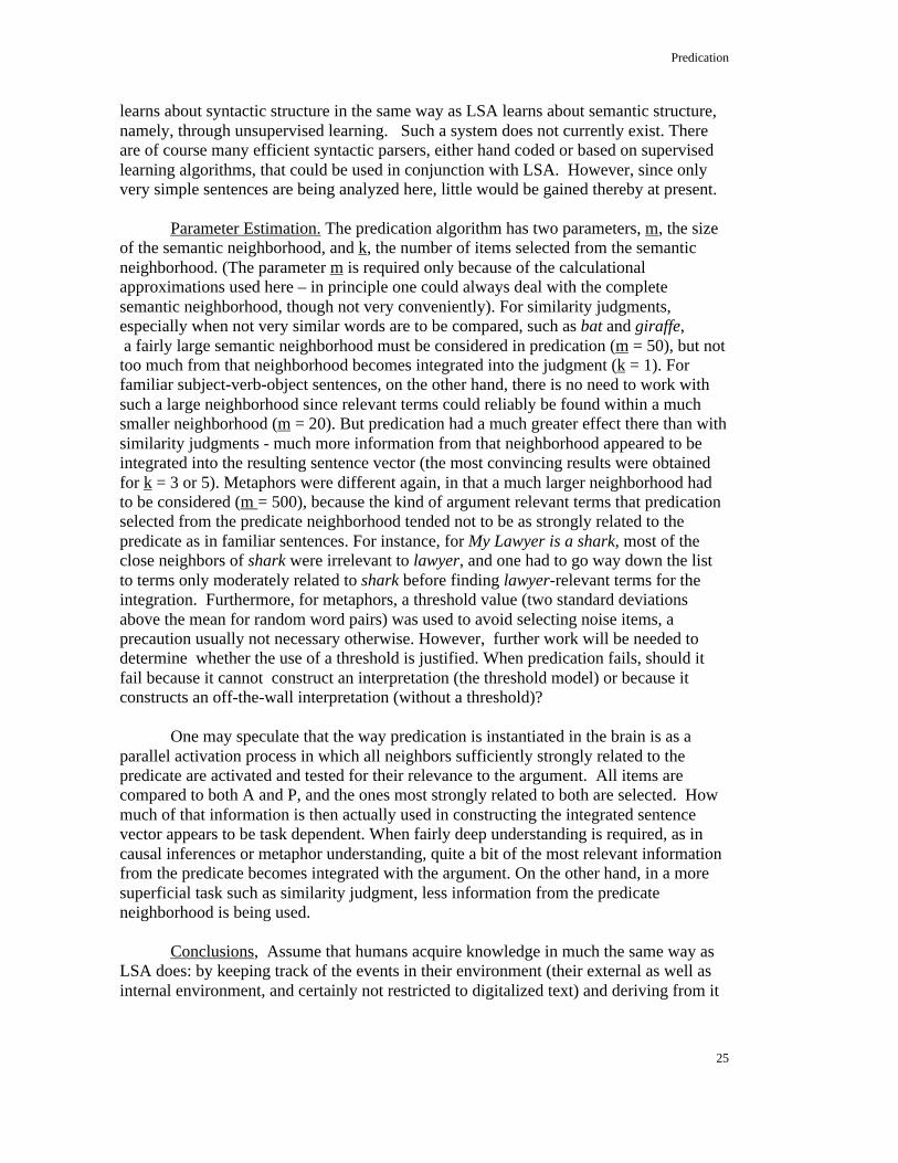
learns about syntactic structure in the same way as LSA learns about semantic structure,namely, through unsupervised learning. Such a system does not currently exist. Thereare of course many efficient syntactic parsers, either hand coded or based on supervisedlearning algorithms, that could be used in conjunction with LSA. However, since onlyvery simple sentences are being analyzed here, little would be gained thereby at present.

Parameter Estimation. The predication algorithm has two parameters, m, the sizeof the semantic neighborhood, and k, the number of items selected from the semanticneighborhood. (The parameter m is required only because of the calculationalapproximations used here – in principle one could always deal with the completesemantic neighborhood, though not very conveniently). For similarity judgments,especially when not very similar words are to be compared, such as bat and giraffe, a fairly large semantic neighborhood must be considered in predication (m = 50), but nottoo much from that neighborhood becomes integrated into the judgment (k = 1). Forfamiliar subject-verb-object sentences, on the other hand, there is no need to work withsuch a large neighborhood since relevant terms could reliably be found within a muchsmaller neighborhood (m = 20). But predication had a much greater effect there than withsimilarity judgments - much more information from that neighborhood appeared to beintegrated into the resulting sentence vector (the most convincing results were obtainedfor k = 3 or 5). Metaphors were different again, in that a much larger neighborhood hadto be considered (m = 500), because the kind of argument relevant terms that predicationselected from the predicate neighborhood tended not to be as strongly related to thepredicate as in familiar sentences. For instance, for My Lawyer is a shark, most of theclose neighbors of shark were irrelevant to lawyer, and one had to go way down the listto terms only moderately related to shark before finding lawyer-relevant terms for theintegration. Furthermore, for metaphors, a threshold value (two standard deviationsabove the mean for random word pairs) was used to avoid selecting noise items, aprecaution usually not necessary otherwise. However, further work will be needed todetermine whether the use of a threshold is justified. When predication fails, should itfail because it cannot construct an interpretation (the threshold model) or because itconstructs an off-the-wall interpretation (without a threshold)?

One may speculate that the way predication is instantiated in the brain is as aparallel activation process in which all neighbors sufficiently strongly related to thepredicate are activated and tested for their relevance to the argument. All items arecompared to both A and P, and the ones most strongly related to both are selected. Howmuch of that information is then actually used in constructing the integrated sentencevector appears to be task dependent. When fairly deep understanding is required, as incausal inferences or metaphor understanding, quite a bit of the most relevant informationfrom the predicate becomes integrated with the argument. On the other hand, in a moresuperficial task such as similarity judgment, less information from the predicateneighborhood is being used.

Conclusions, Assume that humans acquire knowledge in much the same way asLSA does: by keeping track of the events in their environment (their external as well asinternal environment, and certainly not restricted to digitalized text) and deriving from it

Predication

26

a high-dimensional semantic space by an operation like dimension reduction. Thissemantic space serves them as the basis for all cognitive processing. Often cognitiondirectly reflects the properties of this semantic space, as in the many cases where LSAalone has provided good simulations of human cognitive processes. But often cognitiveprocesses operate on this knowledge base, thus transforming it in new ways. One suchcase was explored in the present paper. Predication uses the LSA space to represent staticword knowledge, but by putting a spreading activation net on top of it, it introduces anelement of contextual modification that is characteristic of comprehension processes.Thus, by combining a comprehension model with an LSA knowledge base, a new andmore powerful model was obtained. What we have, however, is still not a completemodel of cognition. We may conjecture that a model of analytic thinking also uses anLSA knowledge base, but in ways as yet unknown. LSA by itself does not account formetaphor comprehension. But LSA in combination with the construction-integrationmodel of comprehension, does. On the other hand, analogical reasoning, for example, isstill beyond the scope of the LSA+comprehension model. To understand an analogyapparently requires more than finding some features in one domain that illuminate theother domain, as in metaphor comprehension, but requires systematic mapping andtranslation processes that require additional computational mechanisms than theconstraint satisfaction process underlying the construction-integration model. Given thepromise of the predication algorithm introduced here, it seems reasonable to keep lookingfor new ways to expand the use of an LSA knowledge base in modeling cognitiveprocesses.

Predication

27

References

Chomsky (1987). Language in a psychological setting. Sophia Linguistica, 22, 1-73.Deerwester, S., Dumais, S. T., Furnas, G. W., Landauer, T. K., &. Harshman, R. (1990).

Indexing by Latent Semantic Analysis. Journal of the American Society forInformation Science, 41, 391-407.

Deese, J. (1961). From the isolated verbal unit to connected discourse. In C. N. Cofer(Ed.) Verbal learning and verbal behavior. New York, NY: McGraw-Hill.

Collins, A. & Quillian, M. (1969). Retrieval time from semantic memory. Journal ofVerbal Learning and Verbal Behavior, 9, 240-247.

Fellbaum, C.(Ed.) (1998.) WordNet: An electronic lexical database. Cambridge,England: Cambridge University Press.

Foltz, P. W., Kintsch, W., & Landauer, T. K. (1998). The measurement of textualcoherence /with Latent Semantic Analysis. Discourse Processes, 25, 285-307.

Gentner, D., & France, I. M. (1988). The verb mutability effect: Studies of thecombinatorial semantics of nouns and verbs. In S. L. Small, G. W. Cottrell, & M.K. Tanenhaus (Eds.), Lexical ambiguity resolution: Perspectives frompsycholinguistics, neuropsychology, and artificial intelligence . San Mateo, CA:Kaufman. Pp. 343-382.

Gernsbacher, M. A., Keysar, B., & Robertson, R. W. (1995). The role of suppression inmetaphor interpretation. Paper presented at the annual meeting of thePsychonomic Society, Los Angeles.

Gibbs, R. W. Jr. (1994). Figurative thought and figurative language. In M. A.Gernsbacher (Ed.), Handbook of psycholinguistics (pp. 411-446). San Diego:Academic Press.

Glucksberg, S. (1998). Understanding metaphors. Current Directions in PsychologicalScience, 7, 39-43.

Glucksberg, S., Gildea, P., & Bookin, H. B. (1982). On understandig nonliteral speech:Can people ignore metaphors? Journal of Verbal Learning and Verbal Behavior,21, 85-98.

Glucksberg, S. & Keysar, B. (1990). Understanding metaphorical comparisons: Beyondsimilarity. Psychological Review, 97, 3-18.

Glucksberg, S., McGlone, M. S., & Manfredini, D. A. (1997). Property attribution inmetaphor comprehension. Journal of Memory and Language, 36, 50-67.

Heit, E. & Rubenstein, J. (1994). Similarity and property effects in inductive reasoning.Journal of Experimental Psychology: Learning, Memory, and Cognition. 20, 411-422

Katz, J. (1972). Semantic theory. New York: Harper & Row.Kintsch, E., Steinhart, D., Stahl, G, Matthews, C, Lamb, R., and the LSA Research Group

(in press). Developing summarization skills through the use of LSA-basedfeedback. Interactive Learning Environments.

Kintsch, W. (1988). The use of knowledge in discourse processing: A construction-integration model. Psychological Review, 95, 163-182.

Kintsch, W. (1998). Comprehension: A paradigm for cognition. New York: CambridgeUniversity Press.

Predication

28

Kintsch, W. (in press). A computational theory of metaphor comprehension.Psychonomic Bulletin & Review.

Kintsch, W., Patel, V. L., & Ericsson, K. A. (1999). The role of Long-Term WorkingMemory in text comprehension. Psychologia, 42, 186-198.

Laham, D. (1997). Latent semantic analysis approaches to categorization. In M. G. Shafto& M. K. Johnson (Eds.), Proceedings of the 19th Annual Conference of theCognitive Science Society (p. 979) Mahwah, NJ: Erlbaum.

Landauer, T. K. (1999). Learning and representing verbal meaning: The latent semanticanalysis theory. Current Directions in Psychological Science, 7, 161-164.

Landauer, T. K. (in preparation) Single representations of multiple meanings in latentsemantic analysis.

Landauer, T. K. & Dumais, S. T. (1997). A solution to Plato's problem: The LatentSemantic Analysis theory of acquisition, induction and representation ofknowledge. Psychological Review, 104, 211-240.

Landauer, T. K., Foltz, P., & Laham, D. (1998). An introduction to Latent SemanticAnalysis. Discourse Processes, 25, 259-284.

Landauer, T. K., Laham, D., Rehder, R., & Schreiner, M. E., (1997). How well canpassage meaning be derived without using word order? A comparison of LatentSemantic Analysis and humans. In M. G. Shafto & P. Langley (Eds.), Proceedingsof the 19th annual meeting of the Cognitive Science Society (pp. 412-417).Mahwah, NJ: Erlbaum.

Lenat, D. & Guha, R. (1990). Building large knowledge-based systems. Reading, MA:Addison-Wesley.

Mervis, C. B., Rips, L., Rosch, E., Shoben, E. J., & Smith, E. E. (1975). Relatedness ofconcepts. Unpublished data.

Miller, G. A. (1996). The science of words. NY: Freeman.Putejovsky, J. (1995). The generative lexicon. Cambridge, MA: MIT Press.Schank, R. (1975) Conceptual information processing. Amsterdam: North Holland.Singer, M., Halldorson, M., Lear, J. C., & Andrusiak, P. (1992). Validation of causal

bridging inferences in discourse understanding. Journal of Memory andLanguage, 31, 507-524.

Till, R. E., Mross, E. F., & Kintsch, W. (1988). Time course of priming for associate andinference words in a discourse context. Memory & Cognition, 16, 283-298.

Tversky, A., & Hutchinson, J. W. (1986). Nearest neighbor analysis of psychologicalspaces. Psychological Review, 93, 3-22.

Wierzbicka, A. (1988) The semantics of grammar. Amsterdam: John Benjamins.Wittgenstein, L. (1953). Philosophical investigations. New York: Macmillan.Wolfe, M. B., Schreiner, M. E., Rehder, R., Laham, D., Foltz, P. W., Landauer, T. K.,

Kintsch, W. (1998). Learning from text: Matching reader and text by LatentSemantic Analysis. Discourse Processes, 25, 309-336.

Predication

29

Table 1. The 20-term neighborhood of ran, with cosines and activation values for horseand color.

neighborsof ran

cosineneighbor:

horse

activationvalue

(horse)

cosineneighbor:

color

activationvalue

(color)ran 0.21 0.46 0.08 0.24jumped 0.17 0.09 0.06 0.00yelled 0.09 0.00 0.04 0.00stopped 0.21 0.46 0.06 0.00went 0.16 0.00 0.07 0.09shouted 0.16 0.00 0.07 0.46running 0.17 0.09 0.04 0.00hid 0.16 0.00 0.04 0.00cried 0.14 0.00 0.05 0.00grabbed 0.14 0.00 0.03 0.00saw 0.19 0.28 0.07 0.09screamed 0.11 0.00 0.05 0.00hurry 0.11 0.00 0.08 0.24looked 0.15 0.00 0.09 0.39yell 0.20 0.37 0.05 0.00came 0.21 0.46 0.08 0.24raced 0.19 0.28 0.06 0.00rushed 0.13 0.00 0.09 0.39down 0.18 0.19 0.11 0.70hopped 0.12 0.00 0.02 0.00

Predication

30

Table 2. Cosines between ran, horse ran, color ran and two landmarks.

LANDMARKS:ran horse ran color ran

gallop .33 .75 .29dissolve .01 .01 .11

Predication

31

Table 3. Cosines between four subject-verb-object sentences and causal inferencescomputed by centroid and predication. Correct inferences are shown in boldface.

The student washed thetable

the student was clean the table was clean

centroid .70 .71predication .62 .83

The student dropped theglass

the student was broken the glass was broken

centroid .76 .66predication .87 .91

The doctor drank the water the doctor was thirsty the water was thirstycentroid .59 .86

predication .83 .78

The hunter shot the elk the hunter was dead the elk was deadcentroid .66 .54

predication .73 .70

Predication

32

Table 4. Rated similarity for pairs of animal names as a function of two instructionalconditions (Anatomy and Behavior); after Heit and Rubenstein (1994). Cosines arecomputed after predicating either “anatomy” or “behavior” about each animal name.

Data Data cosine cosineAnatomy Behavior Anatomy Behavior

1 shark trout 9.56 4.88 0.67 0.482 hawk chicken 6.44 3.08 0.61 0.353 hawk robin 7.29 4.60 0.64 0.374 shark goldfish 5.75 3.60 0.46 0.385 mosquito ladybug 5.43 3.53 0.22 0.156 bat mouse 4.99 3.46 0.18 0.177 mosquito grasshopper 4.43 3.01 0.9 0.908 bee praying mantis 4.43 3.09 0.74 0.609 snake turtle 4.07 3.14 0.52 0.79

10 bee ant 5.15 4.35 0.81 0.4811 snake lizard 6.47 5.96 0.58 0.8612 bat giraffe 2.03 1.64 0.31 0.1613 whale bear 3.29 3.10 0.07 0.0814 whale tuna 5.56 5.87 0.40 0.2615 whale rabbit 2.51 2.83 0.03 0.1216 snake worm 4.90 5.25 0.41 0.5817 bat sparrow 4.81 5.17 0.48 0.1918 bee hummingbird 3.40 6.64 0.40 0.8119 hawk tiger 2.29 5.72 0.14 0.4520 shark wolf 2.32 6.08 0.14 0.2521 mosquito vampire bat 3.19 7.18 0.31 0.44

Predication

33

Figure 1. A fragment of an integration network. Shown are the predicate ran and theargument horse, and three items from the neighborhood of ran. Solid linesindicate positive connections among nodes; dashed lines indicate inhibitoryconnections.

Predication

34

Figure 2. Three sentences with the predicate collapsed compared to landmarks.

0

0.1

0.2

0.3

0.4

0.5

0.6

cosi

ne

brea

k do

wn

failu

re

racerunner collapsed

plans collapsed

bridge collapsed

Predication

35

Figure 3.Cosines between the vectors for pelican and pelican is a bird and fivelandmarks.

0

0.5

1

cosi

ne

bird

pelic

an

sing

bea

utif

ully

eat f

ish

sea

Landmarks

pelican is a bird

pelican

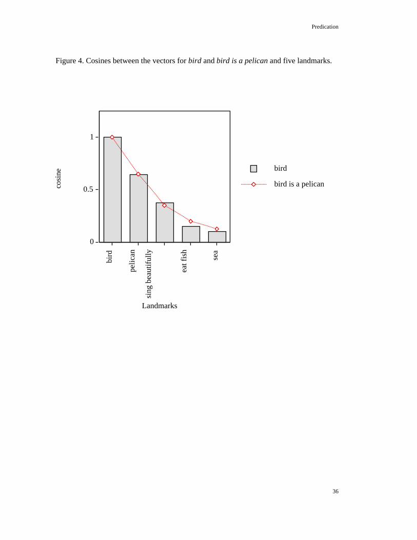
Predication

36

Figure 4. Cosines between the vectors for bird and bird is a pelican and five landmarks.

0

0.5

1

cosi

ne

bird

pelic

an

sing

bea

utif

ully

eat f

ish

sea

Landmarks

bird is a pelican

bird

Predication

37

Figure 5. My lawyer is a shark compared to landmarks.

-25

0

25

50

75

100

cosi

ne

law

yer

just

ice

crim

e

shar

k

fish

vici

ous

Lawyer

My lawyer is a shark

Predication

38

Figure 6. Average differences between rating data and cosines for items rated moresimilar in terms of behavior, neutral items, and items rated more similar in termsof anatomy; data after Heit and Rubenstein (1994).

-0.5

-0.25

0

0.25

0.5

Dif

fere

nce

(Beh

avio

r-A

nato

my)

Behavior Neutral Anatomy.

Cosines

Data

Predication

39

Figure 7. The relationship between three landmarks and the vectors for three sentencesexpressing different senses of mint

0

0.25

0.5

0.75

1

cosi

ne

chocolate stem money

Landmarks

banks mint coins

mint are leaves of a plant

mint is a flavored candy

Predication

40

Footnote

This research was supported by the Army Research Institute and the J. S. McDonnellFoundation. I thank Tom Landauer, Eileen Kintsch, Dave Steinhart and the othermembers of the LSA Research Group for their help, comments, and stimulatingdiscussions.

1 The term feature is used here in a non-technical sense.2 I thank Murray Singer for providing me with these materials.

3 Parameter values used were k=3, m=50.4 Similar low correlations are obtained for free-association matrices. For instance, r = .38 for the

frequency of responses to a list of words related to butterfly (Deese, 1961) and the cosines

between the respective words.

5 In one case the category name in WordNet was unknown to LSA and in another case it

was barely familiar to LSA; the next word listed in the WordNet entry was used as a

substitute.