PREDICATE ANSWER SET PROGRAMMING WITH COINDUCTION

by

Richard Kyunglib Min

APPROVED BY SUPERVISORY COMMITTEE: ___________________________________________ Gopal Gupta, Chair ___________________________________________ Dan Moldovan ___________________________________________ Haim Schweitzer ___________________________________________ Kevin Hamlen

Copyright 2009

Richard Kyunglib Min

All Rights Reserved

I dedicate this work with my gratitude and thanksgiving

to

Mi Min,

Linda Min,

Se June Hong,

and

Samuel Underwood

with my prayer and joy

in

Christ Jesus, our Lord and Savior.

PREDICATE ANSWER SET PROGRAMMING WITH COINDUCTION

by

RICHARD KYUNGLIB MIN, B.S., M.S., M.B.A., M.Div., S.T.M.

DISSERTATION

Presented to the Faculty of

The University of Texas at Dallas

in Partial Fulfillment

of the Requirements

for the Degree of

DOCTOR OF PHILOSOPHY IN

COMPUTER SCIENCE

THE UNIVERSITY OF TEXAS AT DALLAS

August, 2009

v

ACKNOWLEDGEMENTS

I would like to express my gratitude for my advisor Dr. Gopal Gupta, who has been leading

and supporting me and my research to be fruitful in his patience. I would like to thank our

committee members: Dr. Dan Moldovan, Dr. Haim Schweitzer and Dr. Kevin Hamlen,

providing invaluable advices and support, and my colleagues: Dr. Luke Simon, Dr. Ajay

Mallya, and Dr. Ajay Bansal for their valuable research and advices, and especially Dr. Peter

Stuckey whose valuable advice and critiques have helped this research standing on a solid

theoretical foundation, Dr. Melvin Fitting for his advice for Kripke-Kleene 3-valued logic

and stable models, Dr. Farokh Bastani whose meticulous reading and gentle critique

disciplined and shaped my writing and research, Feliks Kluzniak for his reading and critique

on our papers, and Mr. Christ Davis for the final proof reading for our grammar and style.

We are grateful to Dr. Vítor Santos Costa and Dr. Ricardo Rocha for help with implementing

Co-LP on top of YAP, and Mr. Markus Triska for Yap CLP. I thank Dr. Se June Hong who

has given me a life-time opportunity to work under his mentorship and guidance at IBM

Thomas J. Watson Research Center and for his life-long friendship over last twenty-five

years. Finally, I thank my wife Mi, for her persistent love, support, prayer and

encouragement.

May 2009

vi

PREDICATE ANSWER SET PROGRAMMING WITH COINDUCTION

Publication No. ___________________

Richard Kyunglib Min, Ph.D. The University of Texas at Dallas, 2009

Supervising Professor: Gopal Gupta We introduce negation into coinductive logic programming (co-LP) via what we term

Coinductive SLDNF (co-SLDNF) resolution. We present declarative and operational

semantics of co-SLDNF resolution and present their equivalence under the restriction of

rationality and its applications. We apply co-LP with co-SLDNF resolution to Answer Set

Programming (ASP). ASP is a powerful programming paradigm for performing non-

monotonic reasoning within logic programming. The current state of ASP solvers has been

restricted to “grounded range-restricted function-free normal programs”, with a “bottom-up”

evaluation strategy (that is, not goal-driven) until now. The introduction of co-LP with co-

SLDNF resolution has enabled the development of top-down goal evaluation strategies for

ASP. We present a novel and innovative approach to solving ASP programs with co-LP.

Our method eliminates the need for grounding, allows functions, and effectively handles a

large class of predicate ASP programs including possibly infinite ASP programs. Moreover,

it is goal-directed and top-down execution method that provides an innovative and attractive

alternative to current ASP solver technology.

vii

TABLE OF CONTENTS

ACKNOWLEDGMENTS .........................................................................................................v

ABSTRACT ............................................................................................................................. vi

LIST OF FIGURES ................................................................................................................ xi

LIST OF TABLES ....................................................................................................................x

CHAPTER 1 INTRODUCTION .............................................................................................1

1.1 Dissertation Objectives ......................................................................................2

1.2 Dissertation Outline ...........................................................................................3

CHAPTER 2 BACKGROUND ...............................................................................................5

2.1 Mathematical Preliminaries ...............................................................................5

2.2 Logic Programming .........................................................................................14

2.3 Coinductive Logic Programming .....................................................................24

2.4 Answer Set Programming ................................................................................30

CHAPTER 3 COINDUCTIVE LOGIC PROGRAMMING WITH NEGATION ................37

3.1 Negation in Coinductive Logic Programming .................................................37

3.2 Coinductive SLDNF Resolution ......................................................................38

3.3 Declarative Semantics and Correctness Result ................................................50

3.4 Implementation ................................................................................................64

CHAPTER 4 COINDUCTIVE ANSWER SET PROGRAMMING .....................................69

4.1 Introduction ......................................................................................................69

4.2 ASP Solution Strategy .....................................................................................69

4.3 Transforming an ASP Program ........................................................................71

4.4 Coinductive ASP Solver ..................................................................................86

4.5 Correctness of Co-ASP Solver .........................................................................89

CHAPTER 5 APPLICATIONS OF CO-ASP SOLVER ......................................................92

5.1 Introduction ......................................................................................................92

viii

5.2 Simple and Classical ASP Examples ...............................................................93

5.3 Constraint Satisfaction Problems in ASP ......................................................106

5.4 Application to Action and Planning: Yale Shooting Problem .......................110

5.5 Application to Boolean Satisfiability (SAT) Solver ......................................111

5.6 Rational Sequences ........................................................................................120

5.7 Coinductive LTL Solver ................................................................................125

5.8 Coinductive CTL Solver ................................................................................131

CHAPTER 6 PERFORMANCE AND BENCHMARK ......................................................137

6.1 Introduction ....................................................................................................137

6.2 Schur Number ................................................................................................139

6.3 N-Queen Problem ..........................................................................................140

6.4 Yale-Shooting Problem ..................................................................................142

CHAPTER 7 CONCLUSION AND FUTURE WORK ......................................................145

REFERENCES ......................................................................................................................148

VITA

ix

LIST OF FIGURES

Figure 5.1. Predicate-Dependency Graph of Predicate ASP “move-win”. ..............................94

Figure 5.2. Atom-Dependency Graph of Propositional “move-win”. .....................................96

Figure 5.3. Predicate-dependency graph of Predicate ASP “reach” ......................................101

Figure 5.4. Predicate-dependency graph of Predicate ASP abc. ............................................104

Figure 5.5. J2= (ab)(cdef)ω(g)(hijk)ω ......................................................................................122

Figure 5.6. J2= (ab)(cdef)ω(g)(hijk)ω ......................................................................................122

Figure 5.7. Example of ω-Automaton - A1 ...........................................................................123

Figure 5.8. An example of ω-Automaton A2 ........................................................................129

Figure 6.1. Schur 5x12 (I=Size of the query). .......................................................................139

Figure 6.2. Schur BxN (Query size=0). .................................................................................140

Figure 6.3. 8-Queens (I=Size of the query) ...........................................................................141

Figure 6.4. N-Queens. Query size=0 ....................................................................................142

Figure 6.5. Yale Shooting problem (in CPU Seconds). .........................................................143

x

LIST OF TABLES

Table 3.1. Implementation of co-SLDNF atop YAP ...............................................................65

Table 3.2. Implementation of co-SLDNF on top of co-SLD ...................................................66

Table 4.1. Co-ASP Solver (in pseudo-code). ...........................................................................88

Table 5.1. move-win program ..................................................................................................94

Table 5.2. move-win program - ground ...................................................................................95

Table 5.3. move-win program - query examples .....................................................................97

Table 5.4. move-win as a predicate co-ASP program .............................................................99

Table 5.5. reach .....................................................................................................................100

Table 5.6. reach - propositional co-ASP program .................................................................101

Table 5.7. reach - predicate ....................................................................................................103

Table 5.8. ASP program abc for lfp and gfp ..........................................................................104

Table 5.9. co-ASP program for abc .......................................................................................105

Table 5.10. 3-coloring ............................................................................................................106

Table 5.11. 3-coloring ground ...............................................................................................107

Table 5.12. Schur NxB ...........................................................................................................108

Table 5.13. Schur NxB co-ASP program ...............................................................................109

Table 5.14. N-Queens ............................................................................................................110

Table 5.15. Yale-Shooting .....................................................................................................111

Table 5.16. A naïve Boolean SAT solver BSS1 ....................................................................112

Table 5.17. Sample Query Results from BSS1 ......................................................................114

xi

Table 5.18. Boolean SAT solver BSS2 ..................................................................................115

Table 5.19. Boolean SAT solver BSS3 ..................................................................................116

Table 5.20. ASP SAT solver of CNF S .................................................................................117

Table 5.21. co-ASP SAT solver of CNF S ............................................................................117

Table 5.22. co-ASP SAT solver 2 of CNF S .........................................................................118

Table 5.23. co-LP for A1 .......................................................................................................123

Table 5.24. A naïve co-LTL Solver .......................................................................................127

Table 5.25. Co-LP A2 ............................................................................................................130

Table 5.26. Co-LP A2 Sample Queries .................................................................................130

Table 5.27. A naïve co-CTL Solver .......................................................................................132

Table 6.1. Schur 5x12 problem (box=1..5, N=1..12). I=Query size .....................................139

Table 6.2. Schur BxN problem (B=box, N=number) ............................................................140

Table 6.3. 8-Queens problem. I is the size of the query. ......................................................141

Table 6.4. N-Queens problem in CPU sec. Query size = 0 (v2 with minor tuning) ..............141

Table 6.5. A simple Yale Shooting problem (in CPU Seconds). ...........................................142

1

CHAPTER 1

INTRODUCTION

Coinduction is a powerful technique for reasoning about infinite objects and infinite

processes (Barwise and Moss 1996). Coinduction has been recently introduced into logic

programming (termed coinductive logic programming, or co-LP for brevity) by Simon et al.

(2006) with its operational semantics (termed co-SLD resolution) defined for it. Practical

applications of co-LP include goal-directed execution of answer set programs by Gupta et al.

(2007), reasoning about properties of infinite processes and objects, model checking and

verification by Simon et al. (2007). However, co-LP with co-SLD cannot handle negation.

Negation can cause many problems and difficulties in logic programming. One problem is

nonmonotonicity, as one can write programs with negation in cycle where its meaning is not

so intuitive to interpret. For example, a program { p :- not(p). } causes its completion to be

inconsistent. This type of program construct (for example, negation in a cycle) in Answer

Set Programming is not only very common but also posing many problems and difficulties to

keep co-LP with co-SLD or any conventional (logic) programming from being a viable

solution. In this respect, the problems and the challenges with co-LP with co-SLD are two-

fold. First (1), there is a need for co-LP to be extended to handle negation and negation in

cycle. Second (2), co-LP can provide a viable solution to nonmonotonic logic programming

such as Answer Set Programming. These challenges imply the need for the extension of co-

LP where current declarative and operational semantics cannot handle negation and negation

in cycle.

2

1.1 Dissertation Objectives

This dissertation proposes to extend co-LP with negation as failure (naf), in order to provide

a viable solution to handle negation and negation in cycle. It proposes a concrete foundation

for its declarative and operational semantics of co-LP with negation. This work can also be

viewed as extending SLDNF resolution (Lloyd 1987) with coinduction. This work is based

on the author’s previous work with the author’s colleagues (Gupta et al. 2007; Min, Bansal,

and Gupta 2009; Min and Gupta 2009). We term the operational semantics of co-LP

extended with negation as failure as coinductive SLDNF resolution (co-SLDNF). We

propose a comprehensive theory of co-LP with co-SLDNF resolution, implemented on top of

a Prolog engine. In doing so, we have proposed a theoretical framework for declarative

semantics of co-SLDNF adapted from the work of Fitting (1985) with Kripke-Kleene

semantics with 3-valued logic and extended by Fages (1994) for stable model with

completion of program, with the correctness result of co-SLDNF resolution. This provides a

concrete theoretical foundation to handle a (positive or negative) cycle of predicates in

Answer Set Programming (ASP). The techniques and algorithms to solve propositional and

predicate ASP programs are presented. As a result, co-SLDNF resolution constitutes the first

main contribution of this dissertation. The second main contribution of this dissertation is to

provide a viable solution to Answer Set Programming via co-LP with co-SLDNF resolution.

Current solution to ASP is novel and innovative, providing top-down query-driven

interactive coinductive ASP solver (co-ASP solver), contrast to the conventional bottom-up

approach. This result is also very promising as to extend current conventional monotonic

logic programming (for example, Prolog) into nonmonotonic logic programming of ASP via

co-LP with co-SLDNF resolution. The third main contribution of this dissertation is to

3

extend the applications of co-LP with co-SLDNF to Boolean SAT, ω-Automata and

transition system, and model checking with Linear Temporal Logic (LTL) and

Computational Temporal Logic (CTL). Many of these problems are also investigated as the

problems of ASP, to be solved via co-ASP solver. The main contributions of this work are as

follows:

(i) Design of “Coinductive Logic Programming” language extended with negation as

failure (co-LP with co-SLDNF resolution).

(ii) Designing a simple and efficient implementation technique to implement co-LP with

co-SLDNF atop an existing Prolog engine.

(iii) Proof of the correctness (soundness and completeness) of co-SLDNF resolution.

(iv) Design of a top-down algorithm for goal-directed execution of propositional and

predicate Answer-Set Programs.

(v) Design of a simple and efficient implementation technique to implement the top-

down propositional and predicate ASP atop an existing Prolog engine.

(vi) Prototype implementation of co-ASP Solver.

(vii) Proof of the correctness (soundness and completeness) of co-ASP solver.

(viii) Applications of co-LP with co-SLDNF resolution and co-ASP solver in Boolean

SAT, ω-Automata and transition system, and LTL and CTL for model checking.

1.2 Dissertation Outline

The remainder of this dissertation is organized as follows: Chapter 2 presents the

background concepts preliminary for the research presented in this dissertation. It also

presents the literature survey for this research, including co-LP with co-SLD and ASP.

Chapter 3 presents co-LP with co-SLDNF resolution, and its declarative and operational

4

semantics. Chapter 4 presents co-ASP solver and its solution strategy via co-LP. Chapter 5

presents the applications of co-LP to co-ASP applications and related problems including

Boolean SAT, ω-Automata and transition system, model checking with LTL and CTL, and

action and planning in ASP. Chapter 6 presents performance data and implementation,

followed by Chapter 7 Conclusion and Future Works. The two core chapters (Chapters 3 and

4) present the simple and efficient techniques to implement co-LP with co-SLDNF and co-

ASP Solver for propositional and predicate ASP programs atop an existing Prolog engine.

Further, the correctness results for co-SLDNF resolution and co-ASP solver are presented.

5

CHAPTER 2

BACKGROUND

In this chapter we present the requisite concepts and results used throughout this dissertation.

First we overview the requisite basic mathematical concepts and results in section 2.1, logic

programming (LP) in section 2.2, coinductive logic programming (co-LP) with co-SLD

resolution in section 2.3, and finally answer set programming (ASP) in section 2.4. All of

these basic concepts and results are well-known and their detailed presentations are found in

(Barwise and Moss 1996; Aczel 1988; Lloyd 1987; Pierce 2002; Baral 2003; Simon 2006).

Current presentation follows primarily the account of Simon (2006). These basic concepts

and results in this chapter are used implicitly or explicitly throughout this dissertation,

especially to extend co-LP with negation in Chapter 3 and its application to a top-down ASP

solver in Chapter 4.

2.1 Mathematical Preliminaries

In this section, we present the mathematical preliminaries of the basic concepts and results of

fixed points, induction and coinduction. The detailed account is found in Lloyd (1987),

Docets (1993), Barwise and Moss (1996), Pierce (2002), and Simon (2006).

2.1.1 Fixed points

We present the basic concepts and results concerning partial ordering (order-preserving

function), monotonicity, complete lattice, and fixed points, following the presentation of

Lloyd (1987).

6

Let S be a set. A relation R on S is a subset of S×S, and denoted by xRy for (x, y)∈R,

further R is a partial order if (a) xRx for all x ∈ S, (b) xRy and yRx imply x = y for all x, y ∈ S,

and (c) xRy and yRz imply xRz for all x, y, z ∈ S. Adopting the standard notation and using ≤

for partial order, the conditions for partial order are expressed as (a) x ≤ x, (b) x ≤ y and y ≤ x

imply x = y, and (c) x ≤ y and y ≤ z imply x ≤ z, for all x, y, z ∈ S.

Now let S be a set with a partial order ≤. Then m ∈ S is an upper bound of a subset X

of S if x ≤ m, for all x ∈ X. Similarly, n ∈ S is a lower bound of X if n ≤ x, for all x ∈ X.

Further m ∈ S is the least upper bound of a subset X of S if m is an upper bound of X and, for

all upper bounds m' of X, we have m ≤ m'. Similarly, n ∈ S is the greatest lower bound of a

subset X of S if n is a lower bound of X and, for all lower bounds n' of X, we have n' ≤ n. The

least upper bound of X is unique, if exists, and is denoted by lub(X). Similarly the greatest

lower bound of X is unique, if exists, and is denoted by glb(X). Further a partially ordered set

L is a complete lattice if lub(X) and glb(X) exist for every subset X of L.

Now let L be a complete lattice and T : L → L be a mapping. Then we say that (a) T

is monotonic (or order-preserving) if T(x) ≤ T(y) whenever x ≤ y, (b) a subset X of L is

directed if every finite subset of X has an upper bound in X, (c) T is continuous if T(lub(X)) =

lub(T(X)), for every directed subset X of L, and (d) x is a fixed point if T(x) = x. Further we

say that x ∈ L is the least fixed point (lfp for brevity) of T if x is a fixed point and x ≤ y for all

fixed points y of T. Similarly x ∈ L is the greatest fixed point (gfp for brevity) of T if x is a

fixed point and y ≤ x for all fixed points y of T. We recall the following propositions on fixed

points as presented in Lloyd (1987). The reader is referred to Lloyd (1987) for the proofs.

7

Proposition 2.1 (Lloyd 1987): Let L be a complete lattice and T : L → L be monotonic.

Then T has a least fixed point and a greatest fixed point. Furthermore, lfp(T) = glb{ x | T(x) =

x } = glb{ x | T(x) ≤ x } and gfp(T) = lub{ x | T(x) = x } = lub{ x | x ≤ T(x) }.

Proof (Lloyd, 1987). Let G = { x | T(x) ≤ x } and g = glb(G). First we show that g ∈ G. By

definition of g = glb(G), g ≤ x, for all x ∈ G. Further by the monotonicity of T, we have T(g)

≤ T(x) and T(x) ≤ x, for all x ∈ G. Thus T(g) ≤ x, for all x ∈ G. Further by definition of glb,

T(g) ≤ g. Thus g ∈ G. Otherwise, let us suppose that there is x' ∈ G and g ∉ G such that g <

x' ≤ x for all x ∈ G. Then T(g) ≤ T(x') ≤ T(x) for all x ∈ G which is a contradiction that g is

glb(G). Next we show that g is a fixed point of T, that is, g = T(g). Since T(g) ≤ g, it is

sufficient to show that g ≤ T(g). Since T(g) ≤ g implies T(T(g)) ≤ T(g), thus T(g) ∈ G, by

definition of G. Otherwise, if there is y = T(g) ∉ G then T(y) = T(T(g)) ≤ T(g) = y ∉ G,

which is a contradiction. Since T(g) ≤ T(g) and g ≤ T(g), g = T(g), that is, g is a fixed point

of T. Further, let g′ = glb{ x | T(x) = x }. Then g ≤ g′ since g is a fixed point and g′ is glb of

all fixed points of T. Thus g = g′ to complete the proof for lfp(T). The proof for gfp(T) is

similar.

Next we present the basic concepts of ordinal numbers (ordinals for brevity), the

ordinal powers of T, and some of its elementary properties. The first ordinal 0 is defined to

be ∅, the next ordinal is 1 = {∅} = {0}, and 2 = {∅, {∅}} = {0, 1}, and so on. These

comprise all the finite counting ordinals of the non-negative integers. The first infinite

ordinal is ω = {0, 1, 2, …} which is the set of all non-negative integers, followed by ω+1,

ω+2, and so on. Further we can specify an ordering < on the collection of all ordinals by

defining α < β if α ∈ β. That is, (n < n+1) is equivalent to (n ∈ n+1) and (n < ω) is

8

equivalent to (n ∈ ω) for all finite ordinals n and the first infinite ordinal ω. We say that the

ordinal (α+1) to be a successor ordinal of α, and that the ordinal α is a limit ordinal if it is

not the successor of any ordinal. The smallest limit ordinal (other than 0) is ω, and the next

limit ordinal is ω+ω which contains all n and all ω+n where n ∈ ω. Next we present the

principle of transfinite induction followed by the ordinal powers of T as follows: Let P(α)

be a property of ordinals. If, For all ordinals β, P(γ) holds for all γ < β, then P(β) holds.

Then P(α) holds for all ordinals α. Next the definition of the ordinal powers of T is as

follows: Let L be a complete lattice and T : L → L be monotonic. Let ⊤ be the top element

lub(L) and ⊥ be the bottom element glb(L) of L. Further we define: (a) T↑0 = ⊥, (b) T↑α =

T(T↑(α-1)), if α is a successor ordinal, (c) T↑α = lub{ T↑β | β < α}, if α is a limit ordinal, (d)

T↓0 = ⊤, (e) T↓α = T(T↓(α-1)), if α is a successor ordinal, and (f) T↓α = lub{ T↓β | β < α},

if α is a limit ordinal. With this definition of the ordinal powers of T, we note a well-known

characterization of lfp(T) and gfp(T) in terms of ordinal powers of T, as presented by Lloyd

(1987).

Proposition 2.2 (Lloyd 1987): Let L be a complete lattice and T : L → L be monotonic.

Then, for any ordinal α, T↑α ≤ lfp(T) and T↓α ≥ gfp(T). Furthermore, there exist ordinals β1

and β2 such that γ1 ≥ β1 implies T↑γ1 = lfp(T) and γ2 ≥ β2 implies T↓γ2 = gfp(T).

Proof (Lloyd, 1987). The proof for lfp(T) follows from (a) and (e) below. The proofs of (a),

(b) and (c) use transfinite induction.

(a) For all α, T↑α ≤ lfp(T): There are two cases to consider for (i) when α is a limit ordinal,

and (ii) when α is a successor ordinal. For (i), T↑α = lub{ T↑β | β ≤ α} ≤ lfp(T) if α is a

limit ordinal (by the induction hypothesis). For (ii), T↑α = T(T↑(α-1)) ≤ T(lfp(T)) =

9

lfp(T), if α is a successor ordinal (by the induction hypothesis, the monotonicity of T and

the fixed point property).

(b) For all α, T↑α = T↑(α+1): Similar to (a), (i) T↑α = lub{ T↑β | β < α } ≤ lub{ T↑(β+1) | β

< α } ≤ T(lub{ T↑β | β < α }) = T↑(α+1) if α is a limit ordinal, and (ii) T↑α = T(T↑(α-1))

≤ T(T↑α) = T↑(α+1) if α is a successor ordinal.

(c) For all α and β, if α < β then T↑α ≤ T↑β: For (i), if β is a limit ordinal, then T↑α =

lub{ T↑γ | γ < β } = T↑β. For (ii), if β is a successor ordinal, then α ≤ (β - 1) and thus

T↑α ≤ T↑(β - 1) ≤ T↑β, using (b).

(d) For all α and β, if α < β and T↑α = T↑β, then T↑α = lfp(T): Since, by (c), T↑α ≤

T↑(α+1) ≤ T↑β, hence T↑α = T↑(α+1) = T(T↑α) to assert that T↑α is a fixed point, and

further, by (a), T↑α = lfp(T).

(e) There exists β such that γ ≥ β implies T↑γ = lfp(T): Let α be the least ordinal of

cardinality greater than the cardinality of L. Suppose that T↑δ ≠ lfp(T), for all δ < α.

Define h : α → L by h(δ) = T↑(δ). Then by (d), h is injective, which contradicts the

choice of α. Thus T↑β = lfp(T), for some β < α. And the result follows from (a) and (c),

that there exists β such that γ ≥ β implies T↑γ = lfp(T).

For gfp(T), the proof is similar.

The least α such that T↑α = lfp(T) is called the closure ordinal of T. The proof for

proposition 2.2 (also called Knaster-Tarski theorem) is attributed to Knaster for the lattice of

subsets of a set (the power set lattice) and the general proof to Tarski, as noted by Lasses,

Nguyen, and Sonenberg (1982). (Further we label such an operator T as Knaster-Tarski

immediate operator throughout this dissertation.) The next result shows the closure ordinal

10

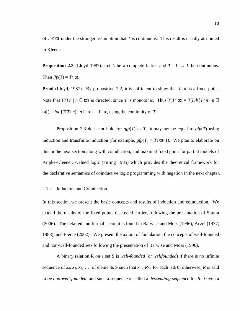
of T ≤ ω, under the stronger assumption that T is continuous. This result is usually attributed

to Kleene.

Proposition 2.3 (Lloyd 1987): Let L be a complete lattice and T : L → L be continuous.

Then lfp(T) = T↑ω.

Proof (Lloyd, 1987). By proposition 2.2, it is sufficient to show that T↑ω is a fixed point.

Note that {T↑n | n ∈ ω} is directed, since T is monotonic. Thus T(T↑ω) = T(lub{ T↑n | n ∈

ω}) = lub{ T(T↑n) | n ∈ ω} = T↑ω, using the continuity of T.

Proposition 2.3 does not hold for gfp(T) as T↓ω may not be equal to gfp(T) using

induction and transfinite induction (for example, gfp(T) = T↓ω+1). We plan to elaborate on

this in the next section along with coinduction, and maximal fixed point for partial models of

Kripke-Kleene 3-valued logic (Fitting 1985) which provides the theoretical framework for

the declarative semantics of coinductive logic programming with negation in the next chapter.

2.1.2 Induction and Coinduction

In this section we present the basic concepts and results of induction and coinduction. We

extend the results of the fixed points discussed earlier, following the presentation of Simon

(2006). The detailed and formal account is found in Barwise and Moss (1996), Aczel (1977;

1988), and Pierce (2002). We present the axiom of foundation, the concepts of well-founded

and non-well-founded sets following the presentation of Barwise and Moss (1996).

A binary relation R on a set S is well-founded (or wellfounded) if there is no infinite

sequence of x0, x1, x2, …. of elements S such that xn+1Rxn for each n ≥ 0; otherwise, R is said

to be non-well-founded, and such a sequence is called a descending sequence for R. Given a

11

membership relationship ∈, a set S is well-founded if S has no infinite descending

membership sequence (S0, …, Sn, Sn+1, …) where ... ∈ Sn+1 ∈ Sn ∈ … ∈ S0 = S. For example,

any finite ordinal is well-founded (as well as ω) with respect to ∈-relation (that is, ≤-relation

as we noted earlier). The axiom for a set to be well-founded with the axiom of choice is

called the axiom of regularity (often called the foundation axiom) which requires every non-

empty set S to contain an element S' which is disjoint from S. Further Two notable results of

the foundation axiom are: (a) no set is an element of itself, and (b) there is no descending

membership sequence of which one of the elements is an element of its successor. For a set

with well-founded relation, transfinite induction can be applied (for example, a set of ordinal

numbers with successor relationship as we noted earlier). Let us consider the set N of natural

numbers and the graph S of the successor function x → x + 1. Here we have mathematical

induction as proof method, recursion as mapping, and lfp (semantics) as definition (meaning

and interpretation). For a set of recursively-defined data structures, we have structural

induction.

However, there are many sets which are not well-founded (or non-well-founded). For

example, rational numbers under partial-ordering is not well-founded because there is no

minimal element, to have infinite descending membership sequence (contrast to its

counterpart example, as we noted earlier, of natural numbers with its minimal element 0).

Further, as we noted earlier, T↓ω with transfinite induction may not be equal to gfp(T).

However, by relaxing the requirement of well-foundedness (also known as the anti-well-

founded axiom), there is a set S such that S ∈ S which is non-well-founded and such a set is

called hyperset. Further if there is a finite sequence x0, x1, x2, …, xk where x0 = xk and xn+1Rxn

for each n ≥ 1 then R is said to be circular and such a sequence is called a cycle. As noted

12

earlier, induction corresponds to well-founded structures that start from a basis which serves

as the foundation for building more complex structures. That is, inductive definition has 3

components: (i) initiality , (ii) iteration, and (iii) minimality. For example, the inductive

definition of a list of numbers is as follows: (i) [] (an empty list) is a list (initiality); (ii)

[H|T] is a list if T is a list and H is some number (iteration); and, (iii) the set of lists is the

minimal set of such lists (minimality). Minimality implies that infinite-length lists of

numbers are not members of the inductively defined set of lists of numbers. Induction

corresponds to least fixed point interpretation of recursive definitions. In contrast,

coinduction to non-well-founded structures is the dual of induction to well-founded

structures. Coinductive definition has 2 components: (i) iteration, and (ii) maximality.

Comparing with induction, coinduction eliminates the initiality condition and replaces the

minimality condition with maximality. Thus, the coinductive definition of a list of numbers

is: (i) [H|T] is a list if T is a list and H is some number (iteration); and, (ii) the set of lists is

the maximal set of such lists (maximality). There is no base case in coinductive definitions.

Using an analogy, it is as if one jumps into a bottomless pit of non-well-founded objects to

follow its infinitely descending sequence without ending and to loop forever in cycle. As we

elaborate later with co-LP, we are especially interested in those finite sequences in cycle (that

is, rational sequences). The objective is to detect its circularity in a finite time (otherwise,

our computation will never terminate in a finite time). Moreover, coinductive definition is

well formed since coinduction corresponds to the greatest fixed point (gfp) interpretation of

recursive definitions. Recursive definition for which gfp interpretation is intended is termed

as corecursive definition. In practice, we may allow the base case in a coinductive definition

13

as we may be interested in all answers, whether it is finite or infinite, which we will elaborate

later with coinductive logic programming.

Finally we summarize these basic concepts with the terms also used in this

dissertation. Let ΓD denote a monotonic function Γ over a domain D. We say that (a) S is Γ-

closed if Γ(S) ⊆ S, (b) S is Γ-justified if S ⊆ Γ(S), and (c) S is a fixed point of Γ if S is both Γ-

closed and Γ-justified. Given a monotonic function Γ, the least fixed point of Γ is the

intersection of all Γ-closed sets, and the greatest fixed point of Γ is the union of all Γ-

justified sets. We denote the least fixed point of Γ by µΓ, and the greatest fixed point by νΓ.

Then the principle of induction is stated as: “if S is Γ-closed, then µΓ ⊆ S”, in contrast to the

principle of coinduction stated as: “if S is Γ-justified, then S ⊆ νΓ”. The proof by

(transfinite) induction is stated as: “if S = {x | Q(x) where Q(x) is a property of x} is Γ-closed,

then every element x of µΓ has the property Q(x)”, in contrast to the proof by coinduction

stated as: “if the characteristic set S = {x | Q(x) where Q(x) is a property} is Γ-justified, then

every element x which has the property Q(x) is also an element of νΓ”.

To summarize, we have overviewed: (1) induction and coinduction, as proof method,

(2) recursion and corecursion, as definition (or mapping), and (3) least fixed point and

greatest fixed point, as formal meaning (semantics). We note the application of coinduction

in many fields of computer science, mathematics, philosophy and linguistics, as noted by

Barwise and Moss (1996), including bisimulation, bisimilarity proof and concurrency (Park

1981; Milner 1989), process algebras (Milner 1980) such as π-calculus (Milner, 1999),

programming language semantics (Milner and Tofte, 1991), model checking (Clarke,

Grumberg, and Doron 1999), situation calculus (Reiter 2001), description logic (Baader et al.

2003), and game theory and modal logic as noted in Barwise and Moss (1996). The

14

extension of logic programming with coinduction allows for both recursion and co-recursion

as discussed in Simon (2006). In this dissertation, we extend co-LP with negation and its

application to solve answer set programs in top-down and query-based manner. Next we

briefly overview logic programming in the next section, followed by its extension to

coinductive logic programming (co-LP) by Simon et al. (2007).

2.2 Logic Programming

Logic Programming (LP) languages belong to the class of programming languages called

declarative programming languages (Scott 2006). Declarative programming languages

intend to reduce the burden and the side-effect caused by many phases of the traditional

imperative (procedural) programming paradigm of (a) the definition and the analysis of the

problem (“what a problem is”) and (b) the design of its solution in an algorithm and its

coding (“how to solve it”). As a result, declarative programming languages tend to provide a

highly sophisticated programming language (for example, of first order logic) accompanied

by its system of evaluation (automated theorem prover). For example, with the language and

system of first-order logic, a program becomes a set of axioms (a theory). Its computation to

a solution is the constructive proof of a goal (query) statement to the program, automatically

generated by its accompanying system of automated theorem prover.

Logic (or logic-based) programming language was first proposed by McCarthy

(1959). The proposal was to use logic to represent declarative knowledge to be processed by

an automated theorem prover. The major breakthrough and progress in automated theorem

proving for first order logic is marked by resolution principle by Robinson (1965) along with

its subsequent development such as linear resolution by Loveland (1970) and SL resolution

by Kowalski and Kuehner (1971). In 1972, the fundamental idea that “logic can be used as a

15

programming language” is conceived by Kowalski and Colmerauer (Lloyd, 1987), with the

proposal of logic programming language (Kowalski, 1974) and the implementation of Prolog

(PROgramming in LOGic) interpreter by Colmerauer and his students in 1972 (Colmerauer

and Roussel, 1996). The conception of Prolog is based on the observation that a subset of

first-order logic (predicate calculus) called Horn’s logic (Horn, 1951) is adequate as a (logic)

programming language, to be efficiently implemented and computed by a computer. Next

we present a brief introduction of the syntax and semantics of logic programming language

based on Horn’s logic, following the presentation of Lloyd (1987) and Simon (2006). We

term this type of logic programming as (traditional or “inductive”) logic programming (LP)

for its basis of “induction” as a proof method, in contrast to coinductive logic programming

(co-LP) due to its extension with “coinduction”, following the convention of Simon (2006).

The theory of LP, as a subset of the theory of first order logic, consists of (a) an alphabet and

a language (of universally quantified Horn’s clauses) with its syntax, and (c) a set of axioms

and a set of inference rules (to derive the theorems) with its semantics.

2.2.1 Syntax of LP

An alphabet of LP consists of the following six classes of symbols: (a) variables, (b)

constants, (c) function symbols, (d) predicate symbols, (e) connectives, and (g) punctuation

symbols. For LP, we assume the collections of constants including all natural numbers,

variables, and function and predicate symbols with an associated arity n ≥ 1. A logic

program consists of rules (called Horn’s clauses) of the form

A0 ← B1, ..., Bn. (2.1)

for some n ≥ 0 where A0, B1, ..., Bn are called atoms (or predicates), A0 is called the head (or

conclusion) of rule (2.2.1), and B1, ... , Bn is called the body (or premises) of rule (2.1). The

16

body is the conjunction of atoms B1, ... , Bn where each atom is separated by a comma

corresponding to the logical operator “∧” (that is, “and”). Each clause is terminated by a

period and the connective “←” between the head and the body is corresponding to the logical

operator of implication (that is, “if”). For a convenience of our notation, we also use { C1, ...,

Cm } to denote a list of clauses C1, ..., Cm, and use “:-” with “←” interchangeably. A rule

without a body is called a fact (or a unit clause) (for example, { A0. }). A rule without a head

is called a query or a goal (for example, { ← B1, ... , Bm. }), and each Bi is called a subgoal.

A literal is an atom or a negated atom. An atom B1 is a positive literal whereas an atom Bi

prefixed with a negation (for example, “not Bi”) is a negative literal. An empty clause is a

clause without head and body, and denoted by ���� (or {}). Further an atom is an expression of

the form p(t1, …, tn) where p is a predicate symbol of arity n (that is, of n arguments) where t1,

…, tn are terms (or arguments). A term is defined recursively as follows: (i) a constant is a

term, (ii) a variable is a term, and (iii) if f is a function symbol with arity of n (that is, n

arguments) and t1,...,tn are terms, then the function f(t1,...,tn) is a term. A term without any

variable is called a ground term, an atom without variable is called a ground atom, and a

clause without any variable is called a ground clause. We denote a function symbol f of arity

n by f/n and a predicate symbol p of arity n by p/n. The set of all clauses with the same

predicate symbol A0 in the head is called the definition of A0. A logic program of a finite set

of definite clauses is called a definite (or positive) program. Extending LP of Horn’s logic, if

negative literal is allowed in the body of a clause then it is called a normal program.

Moreover, if more than one atom is allowed in the head, then the program is called a general

program. The informal meaning of a clause C = { A0 :- B1, ..., Bn. } is that “for each

assignment of each variable in the clause C to make it ground, A0 is true if all of B1, ..., Bn are

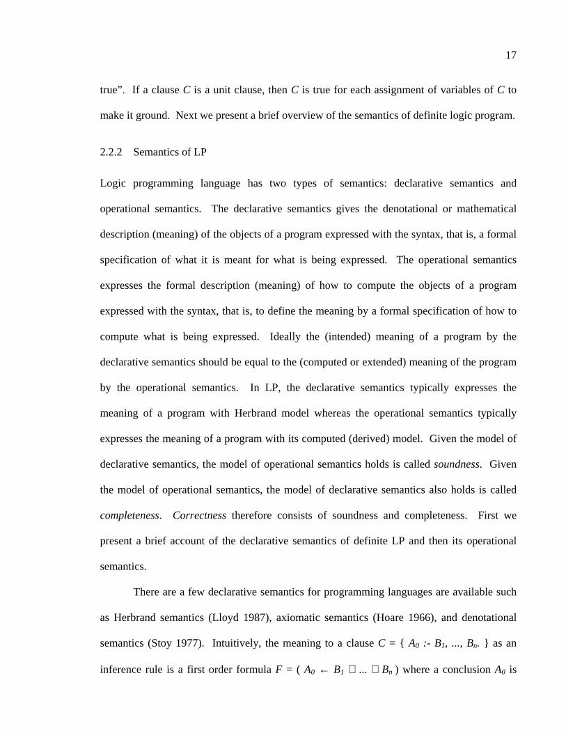
17

true”. If a clause C is a unit clause, then C is true for each assignment of variables of C to

make it ground. Next we present a brief overview of the semantics of definite logic program.

2.2.2 Semantics of LP

Logic programming language has two types of semantics: declarative semantics and

operational semantics. The declarative semantics gives the denotational or mathematical

description (meaning) of the objects of a program expressed with the syntax, that is, a formal

specification of what it is meant for what is being expressed. The operational semantics

expresses the formal description (meaning) of how to compute the objects of a program

expressed with the syntax, that is, to define the meaning by a formal specification of how to

compute what is being expressed. Ideally the (intended) meaning of a program by the

declarative semantics should be equal to the (computed or extended) meaning of the program

by the operational semantics. In LP, the declarative semantics typically expresses the

meaning of a program with Herbrand model whereas the operational semantics typically

expresses the meaning of a program with its computed (derived) model. Given the model of

declarative semantics, the model of operational semantics holds is called soundness. Given

the model of operational semantics, the model of declarative semantics also holds is called

completeness. Correctness therefore consists of soundness and completeness. First we

present a brief account of the declarative semantics of definite LP and then its operational

semantics.

There are a few declarative semantics for programming languages are available such

as Herbrand semantics (Lloyd 1987), axiomatic semantics (Hoare 1966), and denotational

semantics (Stoy 1977). Intuitively, the meaning to a clause C = { A0 :- B1, ..., Bn. } as an

inference rule is a first order formula F = ( A0 ← B1 ∧ ... ∧ Bn ) where a conclusion A0 is

18

inferred by its premises B1, ..., Bn as in the classical logic. One may construct the meaning of

C by composing the meaning of B1 and B2 with the meaning of ∧, and so on (of denotational

semantics which is well-suited for functional programming), or to prove the correctness of

C’s mathematical representation with its pre-condition and post-condition (of axiomatic

semantics which is well-suited for imperative programming). Another way to find a valid

model (meaning) for C out of all the ground clauses of C is to find only those satisfying (of

Herbrand semantics which is well-suited for logic programming). We present a brief

introduction to the declarative semantics of LP is based on the minimal Herbrand model

semantics, following the account of Simon (2006). The detailed account of Herbrand

semantics for LP is found in Lloyd (1987), Apt (1990), Docets (1994), and Simon (2006).

Definition 2.1 (Simon 2006): Let P be a logic program, S(P) be the set of all constant

symbols in P, Fn(P) be the set of all function symbols of arity n (≥ 1) in P.

(a) The Herbrand universe of P, denoted by HU(P), is the set of all finite ground terms of P.

Then HU(P) = µΦp where Φp(S) = S(P) ∪ { f(t1, …, tn) | n ≥ 1, f ∈ Fn(P), t1, …, tn ∈ S}.

(b) The Herbrand base, denoted by HB(P), is the set of all ground atoms that can be formed

from the predicate symbols in P with the elements of HU(P) for the terms.

(c) The Herbrand ground, denoted by HG(P), is the set of all ground clauses { C ← D1, …,

Dn. } of the clauses of P where C, D1, …, Dn ∈ HB(P).

(d) A Herbrand model of P is a fixed-point of TP(S) where TP(S) = {C | (C ← D1, . . . , Dn) ∈

HG(P) ∧ (D1, …, Dn) ∈ S}.

(e) The minimal Herbrand model of P, denoted HM(P), is the least fixed-point of TP, which

exists and is unique according to proposition 2.2. Hence HM(P) is taken to be the

declarative semantics of a traditional logic program P.

19

Here we assume that a program P has a finite set of clauses with non-empty sets of constant

symbols, of function symbols, and of predicate symbols, to avoid a trivial problem. Further

we say Herbrand space, denoted by HS(P), to represent a 3-tuple of (HU(P), HB(P), HG(P))

of P. The Herbrand universe is the set of all enumerable finite ground terms constructed

from the constants and functions in the program. Note that the definition of term can be

viewed as a tree structure whose root node is a function symbol of arity n and its n child-

nodes are the terms defined recursively using constant symbols and terms. Intuitively, HU(P)

assigns a meaning to a term t(X) (in which variables X1, . . . , Xn occurs in t(X) and X =

(X1, . . . , Xn)) by a ground term t of t(X), as a value-assignment to variables. HB(P) assigns a

possible meaning (pre-interpretation) to all predicates of P by their ground instances of

definition. HM(P), a subset of HB(P), assigns a meaning (interpretation) to some of these

ground predicates, a subset of HB(P), to be true. Truth of a ground instance of an atom A is

defined by its inclusion in the model. An atom A of P has a ground instance A’ to be true if

there is a value-assignment to its variables of A to be A’ and A' is in HB(P).

Definition 2.2 (Simon 2006): An atom A of P is true if and only if the set of all groundings

of A of HB(P), with all the substitutions ranging over the HU(P), is a subset of HM(P).

Therefore an atom p(X) of P is true if all groundings of p(X) of HB(P), with all the

substitutions ranging over the HU(P), is a subset of HM(P). Conversely an atom A of P is

not true (that is, false) if and only if there is a set of groundings of A of HB(P), with the

substitutions ranging over the HU(P), is not a subset of HM(P).

The declarative semantics of the minimal Herbrand model provides a meaning (a model) of a

program but does not provide an effective way to compute. For example, let us consider a

simple program P = { p(f(a)). } where P has one predicate symbol p, one function symbol f,

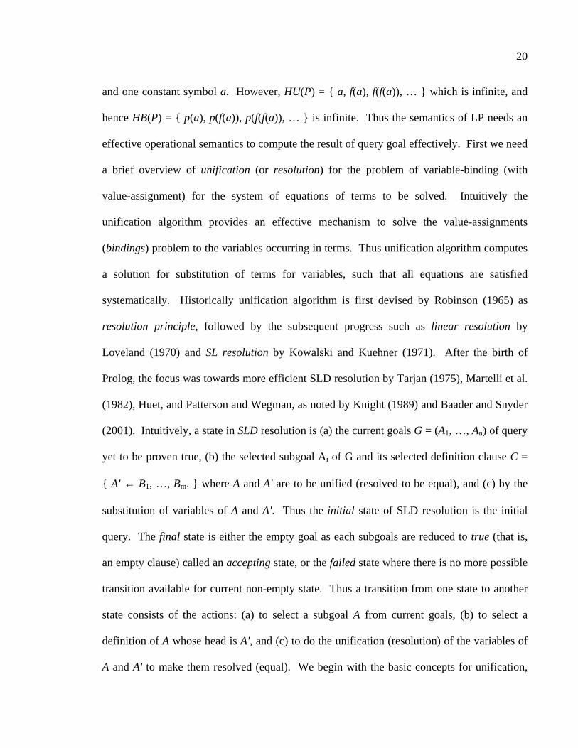
20

and one constant symbol a. However, HU(P) = { a, f(a), f(f(a)), … } which is infinite, and

hence HB(P) = { p(a), p(f(a)), p(f(f(a)), … } is infinite. Thus the semantics of LP needs an

effective operational semantics to compute the result of query goal effectively. First we need

a brief overview of unification (or resolution) for the problem of variable-binding (with

value-assignment) for the system of equations of terms to be solved. Intuitively the

unification algorithm provides an effective mechanism to solve the value-assignments

(bindings) problem to the variables occurring in terms. Thus unification algorithm computes

a solution for substitution of terms for variables, such that all equations are satisfied

systematically. Historically unification algorithm is first devised by Robinson (1965) as

resolution principle, followed by the subsequent progress such as linear resolution by

Loveland (1970) and SL resolution by Kowalski and Kuehner (1971). After the birth of

Prolog, the focus was towards more efficient SLD resolution by Tarjan (1975), Martelli et al.

(1982), Huet, and Patterson and Wegman, as noted by Knight (1989) and Baader and Snyder

(2001). Intuitively, a state in SLD resolution is (a) the current goals G = (A1, …, An) of query

yet to be proven true, (b) the selected subgoal Ai of G and its selected definition clause C =

{ A' ← B1, …, Bm. } where A and A' are to be unified (resolved to be equal), and (c) by the

substitution of variables of A and A'. Thus the initial state of SLD resolution is the initial

query. The final state is either the empty goal as each subgoals are reduced to true (that is,

an empty clause) called an accepting state, or the failed state where there is no more possible

transition available for current non-empty state. Thus a transition from one state to another

state consists of the actions: (a) to select a subgoal A from current goals, (b) to select a

definition of A whose head is A', and (c) to do the unification (resolution) of the variables of

A and A' to make them resolved (equal). We begin with the basic concepts for unification,

21

following the account of Lloyd (1987). An expression is a term, a literal, or a conjunction of

disjunction of literals, whereas a term or an atom is called a simple expression.

Definition 2.3 (Lloyd 1987): Let v1, …, vn be variables, pair-wise distinctive, and t1, …, tn be

terms distinct from vi, and E and F be expressions. Then:

(a) A substitution θ is a finite set {v1/t1, …, vn/tn} where each element vi/ti is called a binding

for vi with ti. If all the ti are variables, then θ is called a variable-pure substitution. If a

substitution is an empty set, it is called an identity substitution.

(b) An instance Eθ is obtained from an expression E with a substitution θ = {v1/t1, …, vn/tn},

by simultaneously replacing each occurrence of the variable vi in E by the term ti where i

= 1, …, n. Further the instance Eθ is called a ground instance of E, if Eθ is ground.

(c) Given substitutions θ1 = {v1/t1, …, vi/ti} and θ2 = {vi+1/ti+1, …, vn/tn}, the composition

θ1θ2 is the substitution obtained from the set {v1/t1θ2, …, vi/tiθ2, vi+1/ti+1, …, vn/tn} by

deleting any binding vj/tjθ2 for which vj = tjθ1 for 1 ≤ j ≤ i, and deleting any binding vk/tk

for which vk ∈ { v1, …, vi } where i+1 ≤ j ≤ n.

(d) If there exist substitutions θ1 and θ2 for E and F such that E = Fθ1 and F = Eθ2, then E

and F are said to be variants where E is a variant of F and F is a variant of E.

(e) A renaming substitution θ = {v1/t1, …, vn/tn} for E is a variable-pure substitution with

pair-wise distinct variable for each ti and not one of variable vj where 1 ≤ i, j ≤ n.

(f) Given S a finite set of simple expressions, a substitution θ is called a unifier for S (or “θ

unifies S”) if Sθ is a set of single element (a singleton). For each unifier σ of S, if there

exists a substitution γ such that σ = θγ, then the unifier θ of S is called a most general

unifier (mgu) for S.

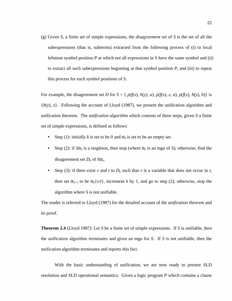
22

(g) Given S, a finite set of simple expressions, the disagreement set of S is the set of all the

subexpressions (that is, subterms) extracted from the following process of (i) to local

leftmost symbol position P at which not all expressions in S have the same symbol and (ii)

to extract all such subexpressions beginning at that symbol position P, and (iii) to repeat

this process for each symbol positions of S.

For example, the disagreement set D for S = { p(f(x), h(y), a), p(f(x), z, a), p(f(x), h(y), b)} is

{ h(y), z}. Following the account of Lloyd (1987), we present the unification algorithm and

unification theorem. The unification algorithm which consists of three steps, given S a finite

set of simple expressions, is defined as follows:

• Step (1): initially k is set to be 0 and σ0 is set to be an empty set.

• Step (2): if Sσk is a singleton, then stop (where σk is an mgu of S); otherwise, find the

disagreement set Dk of Sσk.

• Step (3): if there exist v and t in Dk such that v is a variable that does not occur in t,

then set σk+1 to be σk{ v/t}, increment k by 1, and go to step (2); otherwise, stop the

algorithm where S is not unifiable.

The reader is referred to Lloyd (1987) for the detailed account of the unification theorem and

its proof.

Theorem 2.4 (Lloyd 1987): Let S be a finite set of simple expressions. If S is unifiable, then

the unification algorithm terminates and gives an mgu for S. If S is not unifiable, then the

unification algorithm terminates and reports this fact.

With the basic understanding of unification, we are now ready to present SLD

resolution and SLD operational semantics. Given a logic program P which contains a clause

23

C = { A ← B1, . . . , Bn. }, S be an expression = { A1, …, Ai-1, Ai, Ai+1,… An }, and θ be the

mgu of A and Ai, then a state S make a transition to a state S' = { A1, …, Ai-1, B1, …, Bn, Ai+1,

… An } θ by a transition labeled (C, θ). Such a transition is called as a SLD-transition of P.

Further, with a query Q = { A1, …, An }, the start state of a SLD transition is { A1, … , An },

and the accepting state is {} = ∅. A sequence of SLD transitions (S0, θ0), …, (Sn, θn) where

Si is state and θi is the mgu (for 0 ≤ i ≤ n), to form a path from the start state C0 to some other

state Cn in the system is called SLD derivation. The history of a sequence of transitions from

the initial state is called a trace. If a query Q is successful with the trace of (S0, θ0), …, (Sn,

θn) then the substitution θ0…θn is called the computed answer for Q in P. If a derivation

terminates in the accepting state, then it is a successful derivation. If there is more than one

transition from a state, then it forms a SLD derivation tree whose root node is a starting state

(query). Thus each derivation from a root node forms a branch of a tree, and the last node of

a branch is called a leaf (node). Then the SLD transition system of program P with query Q

consists of the set of states with a starting state of Q, the set of transitions, and the set of

derivations. The SLD semantics provides the model (truth-assignment) to P for all the

successful derivations of Q. Intuitively, a state in SLD derivation is the set of logical

statements (a set of goals) yet to be proven true. If a state is empty, then all the logical

statement of the initial state (the query) is proven to be true. That is, the query has its ground

instance in HM(P) through SLD resolution. Its trace dictates which clause to be selected. Its

computed answer dictates how to ground variables of the initial query to be ground. Thus the

computed answer maps all the terms of the query to be found in HU(P), and all the atoms of

the query to be found in HB(P). Intuitively given the goal of atoms, the SLD operational

semantics dictates the systematic process of what to select and how to ground these clauses

24

whose heads are the goal atoms and whose ground clauses are found in HG(P). There are

two possible instances to be considered: (1) an instance of the ground atoms of the query to

be found in HM(P), to say YES (or SUCCESS), and (2) no ground instance of atoms of the

query in HM(P), to say NO (or FAIL). The reader is referred to Lloyd (1987), Martelli and

Montanari (1982), Knight (1982), Apt (1990), and Baader and Snyder (2001), for the detailed

accounts of the SLD operational semantics and unification, and its history and development.

2.3 Coinductive Logic Programming

Coinductive Logic Programming (Co-LP) provides an operational semantics (similar to SLD

resolution) for computing the greatest fixed point (gfp) of a definite logic program. This

semantics called co-SLD resolution relies on a coinductive hypothesis rule and systematically

computes elements of the gfp of a program via backtracking. The semantics is limited to

only regular (rational) proofs (Colmerauer 1978; Maher 1988; Simon 2006) (that is, for

those cases where the infinite behavior is obtained by infinite repetition of a finite number of

finite behaviors).

2.3.1 Coinductive Hypothesis Rule

The basic concepts of co-LP are based on rational, coinductive proof (Simon et al. 2006), that

are themselves based on the concepts of rational tree and rational solved form of Colmerauer

(1978). A tree is rational if the cardinality of the set of all its subtrees is finite. An object

such as a term, an atom, or a (proof or derivation) tree is said to be rational if it is modeled

(or expressed) as a rational tree. A rational proof of a rational tree is its rational solved form

computed by rational solved form algorithm of Colmerauer (1978), following the account of

Maher (1988) for the axiomatizations and algebras of finite, rational and infinite trees, and

25

some of the key results especially concerning rational trees in relation to infinite trees. The

reader is referred to Colmerauer (1978), and Maher (1988).

A collection of equations over the algebra is to be simplified by the rational solved

form algorithm into a canonical representation of rational solved form. A set of equations

has the form x1 = x2, x2 = x3, …, xn-1 = xn, xn = x1, then it is called circular. If a set of equation

is in the form x1 = t1(x,y), x2 = t2(x,y), …, xn = tn(x,y) where (i) the sets of variables x (that is,

x1, …, xn) and y are disjoint and (ii) the equation set contains no circular subset, then it is in

rational solved form where the variables x are the eliminable variables and the variables y are

the parameters. Some of the noteworthy results for rational trees and its algebra are: (1) the

rational solved form algorithm always terminates, (2) the conjunction of equations E is

solvable iff E has a rational solved form, and (3) the algebra of rational trees and the algebra

of infinite trees are elementarily equivalent.

Further we extend the concept of rational proof of rational trees of terms to the atoms

(predicates) with terms. Further we recall Jaffar and Stukecy (1986), Maher (1988), and

Lloyd (1987) that the equality theory for the algebra of rational trees (for co-LP over the

rational domain) requires one modification to the axioms of the equality theory of the algebra

of finite trees. That is, (i) t(x) ≠ x, for all x and t for each “finite” term t(x) containing x but to

be different from x, and (ii) if t(x) = x then x = t(t(t(...))) for all x and t for each “rational” (an

infinite sequence or stream of t, or a rational tree consisting of two nodes where the root node

points to a node of t and to itself). Note that this modified axiomatization of the equality

theory is required for rational trees, and we will elaborate with a few examples later.

Coinductive proof of a rational (derivation) tree of program P is a rational solved

form (tree-solution) of the rational (derivation) tree. One worthy note is that there is no

26

irrational atom present in the definition of any practical logic programming or any of its

derivations (for example, ASP, Prolog, or co-LP) even though its result at infinity could be

an irrational atom. Further any irrational atom as result of an infinite derivation in this

context should have a rational cover, as noted by Jaffar and Stuckey (1986), which could be

characterized by the (interim) rational atom observed in each step of the derivation. This

observation will be used later to assure some of the results of infinite LP also applicable to

rational LP. Coinductive hypothesis rule (CHR) states that during execution, if the current

resolvent R contains a call C' that unifies with an ancestor call C encountered earlier, then the

call C' succeeds. With this rational feature, co-LP allows programmers to manipulate

rational (finite and rational) structures in a decidable manner as noted earlier.

Definition 2.4 (Colmerauer 1978; Maher 1988; Simon et al. 2006): Let node(A, L) be a

constructor of a tree with root A and subtrees L, where A is an atom and L is a list of trees.

(1) A tree is rational if the cardinality of the set of all its subtrees is finite. An object such as

a term, an atom, or a (proof or derivation) tree is said to be rational if it is modeled (or

expressed) as a rational tree.

(2) A rational proof of a rational tree is its rational solved form computed by rational solved

form algorithm.

(3) A coinductive proof of a rational (derivation) tree of program P is a rational solved form

(tree-solution) of the rational (derivation) tree.

(4) Coinductive hypothesis rule: Simon (2006) states that during execution, if the current

resolvent R contains a call C' that unifies with an ancestor call C encountered earlier, then

the call C' succeeds; the new resolvent is R'θ where θ = mgu(C, C') and R' is obtained by

deleting C' from R.

27

Rational tree (RT) is a special class of infinite trees which has a finite set of subtrees. For

rational tree, rational solved form algorithm (Colmerauer 1978) always terminates and

computes effectively if there exists a solution. With the convention defined above, a rational

term (resp. atom) is then a term (resp. an atom) expressed in a rational tree of finite or

rational constants and functions (resp. terms). With this rational feature, co-LP allows

programmers to manipulate rational (finite and rationally infinite) structures in a decidable

manner. To achieve this feature of the rationality, the unification has to be necessarily

extended, to have “occur-check” removed (Colmerauer, 1978). Unification equations such as

X=[1|X] are allowed in co-LP where X=[1|X] is an infinite sequence or stream of 1, or a

rational tree consisting of two nodes where the root node points to a node of 1 and to itself.

In fact, such equations will be used to represent infinite (regular) structures in a finite

manner.

2.3.2 Co-LP with co-SLD

In this section, we present the declarative and operational semantics of definite co-LP. First

we present co-Herbrand universe, base and model and the declarative and operational

semantics of a definite co-SLD. Following Lloyd (1987), with the (Knaster-Tarski)

immediate-consequence one-step operator TP, we use µ (resp. ν) to denote the least (resp. the

greatest) fixed point operator. We consider only definite (finite) logic program of which

universe, base, and model could be infinite (irrational). We restrict Herbrand universe over

the finite and rational terms (a rational Herbrand Universe), Herbrand base over finite and

rational trees of atoms (a rational Herbrand Base), and Herbrand models over the rational

Herbrand models. Derivations of infinite (irrational) trees of terms or atoms do not terminate

28

in a finite time, and are not computable with a rational solved form, and thus beyond finite

termination whether it is a success or a failure.

Definition 2.5 (Simon 2006) Maximal Herbrand Model of definite co-LP: Let P be a

definite logic program. Let signature Σ be the signature associated with program P. We

define the rational Herbrand Universe of P, HUR(P) = RT(Σ). The rational Herbrand base,

denoted HBR(P), is the set of all ground (finite and rational) atoms that can be formed from

the predicate symbols in P and the elements of HUR(P). Let HGR(P) be the set of ground

clauses of {C ← D1, ..., Dn} that are ground instances of some clause of P such that C, D1,...,

Dn ∈ HBR(P). A rational Herbrand interpretation is a subset of rational Herbrand base and

consists of ground atoms that are true in it. A rational Herbrand model of a logic program P,

denoted HMR(P), is a fixed-point of: TP(S) = {C | C ← D1,..., Dn ∈ HGR(P) ∧ D1,..., Dn ∈ S}.

The Maximal rational Herbrand model of P, denoted Max HMR(P), is the gfp of TP (denoted

νTP or gfp of TP) which exists and is unique. Hence Max HMR(P) is taken to be the

declarative semantics of a coinductive logic program. An atom A is true in a program P if

and only if the set of all groundings of A, with substitutions ranging over HUR(P), is a subset

of Max HMR(P). Thus, P |= A iff A ∈ Max HMR(P).

The declarative semantics of definite co-LP (with co-SLD) is the maximal Herbrand

model, Max HMR(P), defined above. For example, a program { p :- p. q. } has HUR(P)=∅,

HBR(P)={p, q}, HMR(P) = {q} or { p, q}, and thus Max HMR(P) = {p, q}. Next we present

the operational semantics of co-SLD, with co-SLD resolution, followed by co-SLD

derivation and tree. The reader is referred to (Simon 2006; Simon et al. 2007) for the

detailed presentation of co-SLD.

29

Definition 2.6 Co-SLD Resolution (revised from Simon 2006): Co-SLD resolution is defined

as a non-deterministic state transition system where each state is a triple: (G, E, χ) where G is

a finite list of subgoals, E a system of equations (mgu), and χ the coinductive hypothesis

table (list of current ancestor calls). Given a goal A ∈ G currently chosen for evaluation, co-

SLD will: (1) expand subgoal A in G using standard (Prolog-style) logic programming call-

expansion, or (2) delete A, if A ∈ χ (success due to application of the coinductive hypothesis

rule). A derivation is successful if a state is reached in which the subgoal-list is empty. A

derivation fails if a state is reached in which the subgoal-list is non-empty and no transitions

are possible from this state. The initial state is (Q, ∅, ∅), where Q is the list of query

subgoals.

The correctness is proved by equating operational and declarative semantics via soundness

and completeness theorems. The reader is referred to Simon (2006) for the proof of

soundness and completeness of co-SLD.

Theorem 2.5 (Simon 2006) Soundness and Completeness of co-SLD:

(1) Soundness: If the query A1,..., An has a successful derivation in program P, then

E(A1,...,An) is true in program P, where E is the resulting variable bindings for the

derivation.

(2) Completeness: Let A1,..., An ∈ M(P), such that each Ai has a coinductive proof in program

P. Then the query A1, ..., An has a successful derivation in P.

30

2.4 Answer Set Programming

2.4.1 Introduction

Answer Set Programming (ASP) (Gelfond and Lifschitz 1988; Niemelä and Simons 1996;

Baral 2003) is a powerful and elegant way of a declarative knowledge representation and

non-monotonic reasoning in normal logic programming (LP). The origin of ASP could be

found from two areas of research in the semantics of negation as failure (Gelfond and

Lifschitz 1988) and SAT solvers for search problem (Kautz and Salman 1992), and its term

coined by Vldimir Lifschitz (Niemelä 2003). Soon it was recognized as a new programming

paradigm (Lifschitz 1999a; Marek and Truszczyński 1999; Niemelä 1999). Its stable model

semantics is proven to be novel and powerful enough to represent and solve many of the

challenging and difficult problems such as SAT, default logic, constraint satisfaction,

modeling, action and planning (Baral 2003; Niemelä 2003). Some of the interesting recent

applications include planning (Dimopoulos, Nebel, and Koehler. 1997; Lifschitz 1999;

Niemelä 1999), decision support of space shuttle flight controller (Nogueira et al. 2001),

web-based mass-customizing product configuration (Tiihonen et al. 2003), Linux system

configuration for distribution (Syrjänen 1999), verification and model checking (Esparza and

Heljanko 2001; Heljanko 1999; Heljanko and Niemelä 2003), wire routing problem (East and

Truszczyński 2001; Erdem, Lifschitz, and Wong. 2000), diagnosis (Gelfond and Galloway

2001), and network protocol, management and policy analysis (Aiello and Massacci 2001;

Aura, Bishop, and Sniegowski 2000; Son and Lobo 2001).

31

2.4.2 ASP Systems (ASP Solvers)

There have been many powerful and efficient ASP systems (ASP solvers). Some of the

successful ASP systems are: Smodels1 (Niemelä and Simons 1996; Simons, Niemelä and

Soininen 2002), DLV2, Cmodels3, ASSAT4, and NoMoRe5, along with some frontend-

grounding tools such as Lparse6 (Simons and Syrjanen 2003). The Smodels system is one of

very most popular and successful ASP systems. This is also one of the first ASP systems.

Another very powerful and distinctive ASP system is the DLV system of a deductive

database system with its disjunctive logic programming language (disjunctive “Datalog” with

constraints, true negation and query capability). Further the system provides the front-ends

to several knowledge representation formalisms and various database systems including

SQL3. It is very powerful and well suited for nonmonotonic reasoning and tasks including

diagnosis and planning. Another distinctive ASP system is the Cmodels system, with

disjunctive logic programs, using SAT solvers as a search engine to enumerate the models of

a logic program. Similarly the ASSAT (Answer Sets by SAT solvers) system is to compute

ASP using SAT solver(s) from the grounded ASP program. Yet another distinctive and

recent ASP Solver, worthy to mention, is NoMoRe system using tableaux providing a formal

proof system for ASP, with powerful heuristics to prone what is negative. Current ASP

1 http://www.tcs.hut.fi/Software/smodels/

2 http://www.dbai.tuwien.ac.at/proj/dlv

3 http://assat.cs.ust.hk

4 http://www.cs.utexas.edu/users/tag/cmodels.html

5 http://www.cs.uni-potsdam.de/~linke/nomore/

6 http://www.tcs.hut.fi/Software/smodels/

32

Solvers are indeed impressive and competitive to provide an industry-strength power

(Dovier, Formisano, and Pontelli. 2005; Baselice, Bonatti, and Gelfond. 2005) and usability,

competing with the counterpart-systems such as SAT solvers and CLP solvers. In contrast,

all the “full-pledged” ASP solvers without any exception can handle only a class of ASP

programs of “grounded version of a range-restricted function-free normal program” (Niemelä

and Simons 1996). That is, these programs are restricted to be (1) free of positive-loop (for

example, not allowing a rule such as { p :- p. }), (2) range-restricted (a restriction on the

range of variable to be finitely enumerable), and (3) function-free (terms without function

symbols). This imposes a considerable limitation to the class of ASP programs that can be

handled by current ASP solvers. The rationale is intuitive and straightforward, in order to

prevent an explosive and infinite search space. Further this enforces all ASP solvers and thus

ASP solver-strategies, in essence, to be propositional (that is, first to be grounded) and

bottom-up with intelligent heuristics (to prune or split search space). Thus, all of the current

ASP solvers and their solution-strategies, in essence, work for only propositional programs.

These solution strategies are bottom-up (rather than top-down or goal-directed) and employ

intelligent heuristics (enumeration, branch-and-bound or tableau) to reduce the search space.

It was widely believed that it is not possible to develop a goal-driven, top-down ASP Solver

(that is, similar to a query driven Prolog engine). There have been several proposals and

progresses to relax or overcome some or all of these restrictions of current ASP solvers but

still in their premature or early stages (as noted in Bonatti, Pontelli, and Son 2008; Baral

2003; Ferraris and Lifschitz 2005; Ferraris and Lifschitz 2007; Lin and Zhao 2004; Bonatti,

Pontelli, and Son 2008; Pereira and Pinto 2005; Shen, You and Yuan 2004; Janhunen et al.

2006). Some of these attempts and efforts for ASP solver include: (1) function symbols, (2)

33

infinity or loop-positive constructs, and (3) well-founded and partial (stable) model. The

other attempts include: (1) a revision in GLT and ASP, (2) a proposal of ASP in first order,

(3) a proposal for revised stable model (rSM), (4) SLTNF with tabling (in lfp semantics), (5)

loop formulas, and (6) skeptical or credulous ASP (of order-consistent or finitely-recursive

functions odd-cycle-free).

2.4.3 Answer Set Programming

Answer Set Programming (alternatively, A-Prolog by Gelfond M, Lifschitz (1988) and

AnsProlog by Baral (2003)) is a declarative logic programming language. According to

Niemelä (2006), programs are some theories (of some formal system) with a semantics

assigning a collection of sets (or models, referred to as answer sets of the program) to a

theory. Thus one devises a program to solve a problem using ASP, in order that the solutions

of the problem can be derived from the answer sets of the program. The basic syntax of a

ASP program is of the form:

Lo :- L1, … , Lm, not Lm+1, …, not Ln. Rule (1)

where Li is a literal where n ≥ 0 and n ≥ m. In the Answer Set interpretation, this rule states

that Lo must be in the answer set if L1 through Lm, are in the answer set and Lm+1 through Ln

are not in the answer set. If L0 = ⊥ (or null), then its head is null (meant to be false) to force

its body to be false (a constraint rule (Baral 2003) or a headless-rule), written as follows:

:- L1, … , Lm, not Lm+1, …, not Ln. Rule (2)

This constraint rule forbids any answer set from simultaneously containing all of the positive

literals of the body and not containing any of the negated literals.

34

The (stable) models of an answer set program are computed using the Gelfond-

Lifschitz Transformation (GLT) by Gelfond and Lifschitz (1988). Gelfond-Lifschitz

Transformation of Reduct with its recent revision by Ferraris and Lifschitz (2005) is a well-

known and widely-used procedure to find a stable model of a program as follows: Given a

grounded program P and a candidate answer set A, a residual program R is obtained by

applying the following transformation rules: for all literals L ∈ A, (1) to delete all rules in P

which have “not L” in their body, and (2) to delete all “not L” from the bodies of the

remaining rules. The resulting residual program R is called the reduct of the program P.

Then the least fixed point (say, F) of R is computed. If F = A, then A is an answer set for P.

The main difficulty in the execution of answer set programs is caused by the

constraint rules, which are the headless rules above as well as rules of the form as follows:

Lo :- not Lo, L1, … , Lm, not Lm+1, …, not Ln. Rule (3)

Such constraint rules force one or more of the literals L1, …, Lm to be false or one or more

literals “Lm+1, …, Ln” to be true. Note that “not Lo” may be reached indirectly through other

calls when the above rule is invoked in response to the call Lo. Such rules are said to contain

an odd-cycle in the predicate dependency graph (Fages 1994) which is defined next. The

predicate dependency graph of a ASP program is a directed graph consisting of the nodes

(the predicate symbols) and the signed (positive or negative) edges between nodes, where

(for example, using the clause as in Rule (1)) a positive edge is formed from a node Li (where

1 ≤ i ≤ m) in the body of Rule (1) to its head node L0, and a negative edge is formed from a

node Lj (where m+1 ≤ j ≤ n) in the body to its head node L0. Li depends evenly (oddly, resp.)

on Lj if there is a path in the predicate dependency graph from Li to Lj with an even (odd,

resp.) number of negative edges. A predicate ASP program is call-consistent if no node

35

depends oddly on itself. The atom dependency graph is very similar to the predicate

dependency graph but to use the ground instance of the program where its nodes are the

ground atoms and its positive and negative edges are defined with the ground instances of the

program. A predicate ASP program is order-consistent if the dependency relations of its

atom dependency graph is well-founded (that is, finite and acyclic).

Along with this basic rules and syntax (with a single atom in the head like Prolog),

there are a few more syntactic extensions and conventions currently in use of ASP (Simons,

Niemelä, and Soininen 2002; Simons and Syrjanen 2003). First, it is a constraint-rule

(cardinality constraint) to specify a bound or a threshold number (its low or its low-and-high

range) for the number of the literals (the positive or negative atoms in the body) to be true to

make a rule head to be true (for example, a :- 2{b, not c, d, e}3 ). Second, it is a

choice-rule (exclusive-or conclusion) of more than one atom in the head for a disjunctive

logic of exclusive-or conclusion (for example, { a, b, c } :- e, f, not g. ).

Third, it is a weight-rule (weight constraint) to provide a weight (or a list of of the literals in

the rule body or head), (for example, a :- 3 [ b=1, not c=2 ]. ). Finally, it is a

minimize-rule (minimization criteria) to minimize the sum of all the weights assigned

explicitly to the literals, to provide an optimization. Likewise, a maximize-rule can be

achieved by negating all literals in the body of a minimize-rule. There are a few more

conventional features and provisions including constant and range, classical negation, use of

arithmetic in rule, anonymous variables, and others. Most of these extensions can be

expressed in a conventional Prolog without much difficulty, including a second order

operator like “setof” operator for checking cardinality, “either A or B” (“A; B ”), “if A then

B else C” (“A->B;C ”), and Prolog extensions to tabling and constraint logic programming.

36

In this dissertation, we restrict the scope of our study to the basic rule of ASP with a head of

zero or one positive literal.

37

CHAPTER 3

COINDUCTIVE LOGIC PROGRAMMING WITH NEGATION

3.1 Negation in Coinductive Logic Programming

Negation causes many problems and challenges in logic programming (for example,

nonmonotonicity). For example, one can write programs whose meaning is hard to interpret

and whose completion is inconsistent (for example, { p :- not p. }). From this point, we refer

all logic programs to be normal (with zero or more negative literals in the body of a clause,

and one atom for the head) and finite (finite set of clauses with a finite set of alphabets). We

use the notation nt(A) to denote negation as failure (naf) for a coinductive atom A; and nt(A)

is termed a naf-literal. Without occurs-check, the unification equation X = f(X) means that X

is bound to f(f(f( .... ))) (an infinite rational term).

Definition 3.1 (Syntax of co-LP with negation as failure): A coinductive logic program P is

syntactically identical to a traditional (that is, inductive) logic program. However, predicates

executed with co-SLD resolution (gfp semantics restricted to rational proofs) are declared as

coinductive; all other predicates are assumed to be inductive (that is, lfp semantics is

assumed). The syntax of declaring a clause for a coinductive predicate A of arity n is as

follows:

coinductive (A/n).

A :- L 1, ..., L i ,...,L m.

38

where m ≥ 0 and A is an atom (of arity n) of a normal program P. L i is a positive or naf-

literal where 0 ≤ i ≤ m. If m = 0, A is a fact. The naf-literal of A is in the form of nt(A) . �

Next we extend co-SLD resolution so that naf-goals can also be executed. The extended

operational semantics is termed co-SLDNF resolution. The major considerations for

incorporating negation into co-SLD resolution are:

(1) negation as failure: infer nt(p) if p fails and vice versa, that is, nt(p) fails if p succeeds;

(2) negative coinductive hypothesis rule: infer nt(p) if nt(p) is encountered again in the

process of establishing nt(p);

(3) consistency in negation, infer p from double negation, that is, nt(nt(p)) = p.

3.2 Coinductive SLDNF Resolution

Co-SLDNF resolution extends co-SLD resolution with negation. Essentially, it augments co-

SLD with the negative coinductive hypothesis rule which states that “if a negated call nt(p) is

encountered during resolution, and another call to nt(p) has been seen before in the same

computation, then nt(p) coinductively succeeds”. To implement co-SLDNF, the set of

positive and negative calls has to be maintained in the positive hypothesis table (denoted χ+)

and negative hypothesis table (denoted χ+-) respectively.

The operational semantics given for co-LP with negation as failure is defined as an

interleaving of co-SLD and negation as failure for the co-Herbrand model. Extending

co-SLD to co-SLDNF, the goal { nt(A) } succeeds (or has a successful derivation) if { A }

fails; likewise, the goal of { nt(A) } fails (or has a failure derivation) if the goal { A }

succeeds. We restrict P ∪ {A} to be allowed (Lloyd 1987) to prevent floundering in order to

ensure soundness. We also restrict ourselves to the rational Herbrand space. Since naf-

39

literals may be nested, one must keep track of the context of each predicate occurring in the

body of a clause (that is, whether it is in the scope of odd or even number of negations). If a

predicate is under the scope of even number of negations, it is said to occur in positive

context, else it occurs in negative context. Intuitively, a predicate in the scope of an even

number of negation must behave as a positive literal. Henceforth, a positive literal will refer

to all predicates that occur in the scope of an even number of negations. Likewise, a negative

literal will refer to all predicates that occur in the scope of an odd number of negations.

In co-SLDNF, one keeps track of the context of a goal (that is, whether it is in the

scope of odd or even number of negations). If a goal is under the scope of even number of

negations, it is said to occur in positive context, else it occurs in negative context. In

co-SLDNF, we will also have to remember negated goals since negated goals can also

succeed coinductively. Thus, the state is represented as (G, E, χ+, χ-) where G is the subgoal

list (containing positive or negated goals), E is a system of term equations, χ+ is the set of

ancestor calls occurring in positive context (that is, in the scope of zero or an even number of

negations), and χ- is the set of ancestor calls occurring in negative context (that is, in the

scope of an odd number of negations). From one state, an action of co-SLDNF resolution

will be executed to make a transition into the next state. The sequence of the states in the

transition is co-SLDNF derivation. For the definition of co-SLDNF resolution, we need a

few more requisite concepts as follows:

Definition 3.2 Given a co-LP P and an atom A in a query goal G, the set of all clauses with

the same predicate symbol A in the head is called the definition of A. The unifiable-definition

of A is the set of all clauses of Ci = { Hi :- Bi } (where 1 ≤ i ≤ n) where A is unifiable with Hi.

Each Ci of the unifiable-definition of A is called a candidate clause for A. Each candidate

40

clause Ci of the form {Hi(ti) :- Bi.} is modified to {Hi(xi) :- xi = ti, Bi.}, where (xi = ti, Bi)

refers to the extended body of the candidate clause, ti is an n-tuple representing the arguments

of the head of the clause Ci, Bi is a conjunction of goals, and xi is an n-tuple of fresh unbound

variables (that is, standardization apart). Let Si be the extended body of the candidate clause

Ci (that is, Si is (xi = ti, Bi), for each i where 1 ≤ i ≤ n). Then an extension Gi of G for A in

negative context with respect to Si is obtained by replacing A with Siθi where θi = mgu(A, Hi).

The complete-extension G′ of G for A in negative context is obtained by the conjunction of

the extension Gi for each Si where 1 ≤ i ≤ n. If there is no definition for A in P, then the

complete-extension G′ of G for A in negative context is obtained by replacing A with false. �

For example, given G = nt(D1, A, D2) with the n-candidate clauses for A where its extended

body is Si(xi) where 1 ≤ i ≤ n. Then the complete-extension G′ of G for A will be: G′ =

(nt(D1, S1(x1)θ1, D2), …, nt(D1, Sn(xn)θn, D2)). Intuitively, the concept of the complete-

extension captures the idea of negation as failure that the proof of A in negative context (that

is, a negative subgoal, ¬A) requires the failure of all the possibilities of A. That is, ¬A ↔

¬(H1 ∨ … ∨ Hn) ↔ (¬H1 ∧ … ∧ ¬Hn) where Hi is a candidate clause of A. In contrast, the

proof of A in positive context (for a possibility of Hi for some i). Thus the complete-

extension embraces naturally the dual concepts of (i) the negation of the disjunctive subgoals

(the disjunction in negative context) with (ii) the conjunction of the negated subgoals. For

example, nt(D1, (S1(x1)θ1 ∨ … ∨ Sn(xn)θn), D2) is equivalent to (nt(D1, S1(x1)θ1, D2), …,

nt(D1, Sn(xn)θn, D2))). We are now ready to define co-SLDNF resolution.

Definition 3.3 Co-SLDNF Resolution: Suppose we are in the state (G, E, χ+, χ-) where G is

a list of goals containing an atom A, and E is a set of substitutions (environment).

41

(1) If A occurs in positive context, and A' ∈ χ+ such that θ = mgu(A, A'), then the next state

is (G', Eθ, χ+, χ-), where G' is obtained by replacing A with ����.

(2) If A occurs in negative context, and A' ∈ χ- such that θ = mgu(A, A'), then the next state

is (G', Eθ, χ+, χ-), where G' is obtained by A with false.

(3) If A occurs in positive context, and A' ∈ χ- such that θ = mgu(A, A'), then the next state is

(G', E, χ+, χ-), where G' is obtained by replacing A with false.

(4) If A occurs in negative context, and A' ∈ χ+ such that θ = mgu(A, A'), then the next state

is (G', E, χ+, χ-), where G' is obtained by replacing A with ����.

(5) If A occurs in positive context and there is no A' ∈ (χ+ ∪ χ-) that unifies with A, then the

next state is (G', E', {A} ∪χ+, χ-) where G' is obtained by expanding A in G via normal

call expansion using a (nondeterministically chosen) clause Ci (where 1≤ i ≤ n) whose

head atom is unifiable with A with E' as the new system of equations obtained.

(6) If A occurs in negative context and there is no A' ∈ (χ+ ∪ χ-) that unifies with A, then the

next state is (G', E', χ+, {A} ∪ χ-) where G' is obtained by the complete-extension of G

for A.

(7) If A occurs in positive or negative context and there are no matching clauses for A, and

there is no A' ∈ (χ+ ∪ χ-) such that A and A' are unifiable, then the next state is (G', E,

χ+, {A} ∪ χ-), where G' is obtained by replacing A with false.

(8) (a) nt(…, false, …) reduces to ����, (b) nt(A, ����, B) reduces to nt(A, B) where A and B

represent conjunction of subgoals, and (c) nt(����) reduces to false.

Note that the result of expanding a subgoal with a unit clause in step (5) and (6) is an empty

clause (����). When an initial query goal reduces to an empty clause (����), it denotes a success

42

(denoted by [success]) with the corresponding E as the solution. When an initial query goal

reduces to false, it denotes a fail (denoted by [fail]). �

Co-SLDNF derivation of the goal G of program P is a sequence of co-SLDNF resolution

steps (of Definition 3.3), defined as follows:

Definition 3.4 Co-SLDNF derivation:

(1) Co-SLDNF derivation of the goal G of program P is a sequence of co-SLDNF resolution

steps (of Definition 3.3) with a selected subgoal A, consisting of a sequence (Gi, Ei, χi+,

χi-) of state (i ≥ 0), of (a) a sequence G0, G1, ... of goal, (b) a sequence E0, E1, ... of mgu's,

(c) a sequence χ0+, χ1+, ... of the positive hypothesis table, and (d) χ0-, χ1-, ... of the

negative hypothesis table, where (G0, E0, χ0+, χ0-) = (G, ∅, ∅, ∅) as the initial state, and

(e) for the steps (5) and (6) of Definition 3.3, a sequence C1, C2, ... of variants of program

clauses of P where Gi+1 is derived from Gi and Ci+1 using θi+1 where Ei+1 = Eiθi+1 and

(χi+1+, χi+1-) as its resulting positive and negative hypothesis tables.

(2) If a co-SLDNF derivation from G results in an empty clause of query ����, that is, the final

state of (����, Ei, χi+, χi-), then it is a successful co-SLDNF derivation. A co-SLDNF

derivation fails if a state is reached in the subgoal-list which is non-empty and no

transitions are possible from this state (as defined in Definition 3.3).

(3) Success Set [SS] and Finite-Failure Set [FF] are defined as follows:

(a) [SS]={ A | A ∈ HBR(P), the goal { A } →* ���� }

(b) [FF]={ A | A ∈ HBR(P), the goal { nt(A) } →* ���� }

43

where →* denotes a co-SLDNF derivation of length 0 or more, and ���� denotes an empty

clause {}. The third possibility is an irrational (infinite) derivation, considered to be

undefined in the rational space. �

There could be more than one derivation from a node if there is more than one step available

for the selected subgoal (for example, many clauses are applicable for the expansion rules of

steps (5) and (6) in Definition 3.3). A co-SLDNF resolution step may involve expanding

with a program clause for steps (5) and (6) in Definition 3.3 with the initial goal G = G0. The

initial state of (G0, E0, χ0+, χ0-) = (G, ∅, ∅, ∅), and Ei+1 = Eiθi+1 (and so on) may look as

follows:

C1,θ1 C2,θ2 C3,θ3 (G0, E0, χ0+, χ0-) → (G1, E1, χ1+, χ1-) → (G2, E2, χ2+, χ2-) → ...

Further for sake of the notational simplicity and shortcut, we use the disjunctive form for step

(6) in Definition 3.3 instead of the conjunctive form. For example, nt(D1, (S1(x1)θ1; … ;

Sn(xn)θn), D2) is used for (nt(D1, S1(x1)θ1, D2), …, nt(D1, Sn(xn)θn, D2))) where “∨” is denoted

by “; ” as we adapt the conventional Prolog disjunctive operator for a convenience. We also

use the bold font to denote inline program code (for example, a query or an atom).

Example 3.1 Consider the following program NP1:

NP1: p :- nt(q).

q :- nt(p).

First (1), consider the query Q1 = ?- p resulting in the following derivation:

({p}, {}, {}, {}) by (5)

→ ({nt(q)}, {}, {p},{}) by (6)

→ ({nt(nt(p))}, {}, {p}, {q}) by (1)

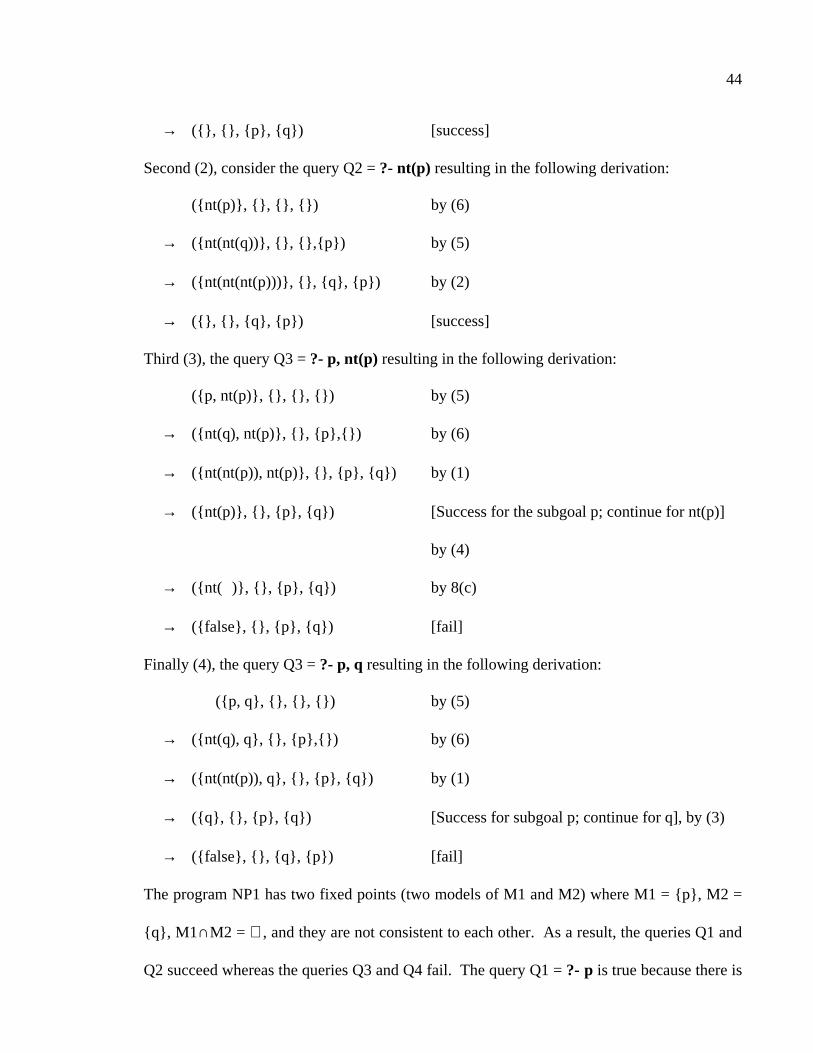
44

→ ({}, {}, {p}, {q}) [success]

Second (2), consider the query Q2 = ?- nt(p) resulting in the following derivation:

({nt(p)}, {}, {}, {}) by (6)

→ ({nt(nt(q))}, {}, {},{p}) by (5)

→ ({nt(nt(nt(p)))}, {}, {q}, {p}) by (2)

→ ({}, {}, {q}, {p}) [success]

Third (3), the query Q3 = ?- p, nt(p) resulting in the following derivation:

({p, nt(p)}, {}, {}, {}) by (5)

→ ({nt(q), nt(p)}, {}, {p},{}) by (6)

→ ({nt(nt(p)), nt(p)}, {}, {p}, {q}) by (1)

→ ({nt(p)}, {}, {p}, {q}) [Success for the subgoal p; continue for nt(p)]

by (4)

→ ({nt(����)}, {}, {p}, {q}) by 8(c)

→ ({false}, {}, {p}, {q}) [fail]

Finally (4), the query Q3 = ?- p, q resulting in the following derivation:

({p, q}, {}, {}, {}) by (5)

→ ({nt(q), q}, {}, {p},{}) by (6)

→ ({nt(nt(p)), q}, {}, {p}, {q}) by (1)

→ ({q}, {}, {p}, {q}) [Success for subgoal p; continue for q], by (3)

→ ({false}, {}, {q}, {p}) [fail]

The program NP1 has two fixed points (two models of M1 and M2) where M1 = {p}, M2 =

{q}, M1 ∩M2 = ∅, and they are not consistent to each other. As a result, the queries Q1 and

Q2 succeed whereas the queries Q3 and Q4 fail. The query Q1 = ?- p is true because there is

45

a model M1 = {p}. The query Q2 = ?- nt(p) is true because there is a model M2 = {q}. For

this reason, computing with (greatest or maximal) fixed point semantics (the partial models)

in presence of negation could be troublesome and seemingly to be perceived as contradictory.

Consequently one has to be careful that given a query, different parts of the query are not to

be computed with respect to different fixed points. Moreover, the query ?-p, nt(p) will never

succeed if we are aware of the context (of a particular fixed point being used). However, if

the subgoals p and nt(p) are evaluated separately and the results conjoined without enforcing

their consistency, then it will wrongly succeed. To ensure consistency of the partial

interpretation, the sets χ+ and χ- are employed in our operational semantics; they in effect

keep track of the particular fixed point(s) under use.

Example 3.2 Consider the following program NP2:

NP2: p :- p.

First (1), consider the query Q1 = ?- p and its derivation as follows:

({p}, {}, {}, {}) by (5)

→ ({p}, {}, {p},{}) by (1)

→ ({}, {}, {p}, {}) [success]

Second (2), consider the query Q2 = ?- nt(p) and its derivation as follows:

({nt(p)}, {}, {}, {}) by (6)

→ ({nt(p)}, {}, {},{p}) by (2)

→ ({nt(false)}, {}, {}, {p}) by (8a)

→ ({}, {}, {q}, {p}) [success]

Third (3), consider the query Q3 = ?- p, nt(p) and its derivation as follows:

({p, nt(p)}, {}, {}, {}) by (5)

46

→ ({p, nt(p)}, {}, {p},{}) by (1)

→ ({nt(p)}, {}, {p}, {}) [success for subgoal p; continue with nt(p)] by (4)

→ ({nt(����)}, {}, {p}, {q}) by (8c)

→ ({false}, {}, {p}, {q}) [fail]

Both queries Q1 and Q2 succeed with NP2. The program NP2 has two fixed points (or two

models) M1 and M2 where M1 = {p}, and M2 = {}. Further M1 ∩ M2 = ∅ and M2 ⊆ M1

where M1 is the greatest fixed point of NP2 and M2 is the least fixed point of NP2. As we

noted, the query ?- nt(p) is true in M2 = {} because nt(p) is true in M2, while the query ?- p

is true in {p} as p is true in M1. This type of the behavior of co-LP with co-SLDNF seems

to be confusing and counter-intuitive. However, as we noted earlier with NP1, this type of

the behavior of co-LP with co-SLDNF is indeed advantageous as we extend the capability of

the traditional LP into the realm of the modal and nonmonotonic reasoning. Clearly, the

addition of a clause like { p :- p. } to a program extends each of its initial models into two

models where one includes p and the other does not include p. However, co-SLDNF

enforces consistency and therefore the query ?- p, nt(p) will fail. Further, for sake of the

explorative experiment, let us allow the Boolean operator OR (or “∨”) which will be “;” (that

is, Prolog’s OR-operator). Note that the “;” operator in Co-LP (as in Prolog) is syntactic

sugar in that (P ; Q) is defined as:

P;Q :- P.

P;Q :- Q.

where a query goal (���� ; A) = (A ; ����) = ���� (an empty clause), and (false ; A) = (A ; false) = A.

Finally (4), consider the query Q4 = ?- (p; nt(p)) which will generate the following transition

sequence with the program NP2:

47

({p ; nt(p)}, {}, {}, {}) by (5)

→ ({p ; nt(p)}, {}, {p},{}) by (1)

→ ({���� ; nt(p)}, {}, {p}, {}) [success for subgoal p; continue with nt(p)]

by (4)

→ ({}, {}, {p}, {q}) [success]

Example 3.3 Consider the following program NP3:

Let us consider the following program NP3 (to be compared with NP2).

NP3: p :- nt(p).

First (1), consider the query Q1 = ?- p with NP3 and its derivation as follows:

({p}, {}, {}, {}) by (5)

→ ({nt(p)}, {}, {p},{}) by (4)

→ ({nt(����)}, {}, {p}, {}) by (8c)

→ ({false}, {}, {p}, {}) [fail]

Second (2), consider the query Q2 = ?- nt(p) and its derivation as follows:

({nt(p)}, {}, {}, {}) by (6)

→ ({nt(nt(p))}, {}, {},{p}) by (3)

→ ({nt(nt(false))}, {}, {}, {p}) by (8a)

→ ({nt(����)}, {}, {q}, {p}) by (8c)

→ ({false}, {}, {q}, {p}) [fail]

Third (3), consider the query Q3 = ?- (p; nt(p)) and its derivation as follows:

({p ; nt(p)}, {}, {}, {}) by (5)

→ ({nt(p); nt(p)}, {}, {p},{}) by (4)

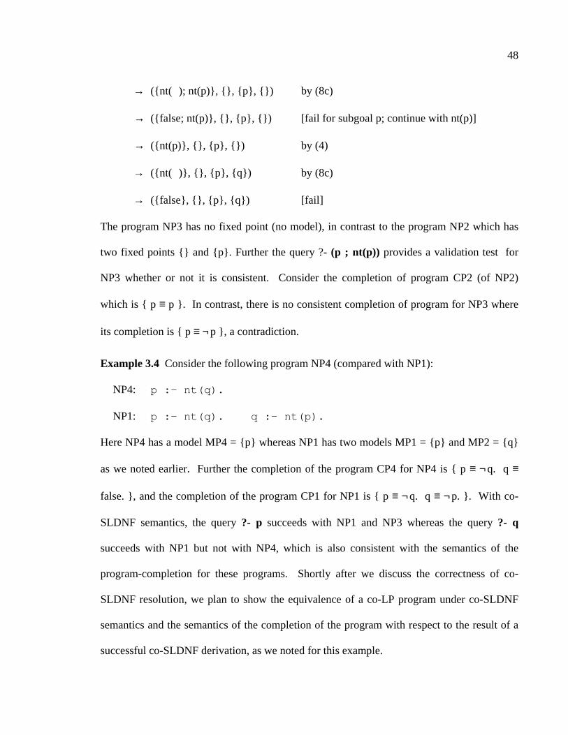
48

→ ({nt(����); nt(p)}, {}, {p}, {}) by (8c)

→ ({false; nt(p)}, {}, {p}, {}) [fail for subgoal p; continue with nt(p)]

→ ({nt(p)}, {}, {p}, {}) by (4)

→ ({nt(����)}, {}, {p}, {q}) by (8c)

→ ({false}, {}, {p}, {q}) [fail]

The program NP3 has no fixed point (no model), in contrast to the program NP2 which has

two fixed points {} and {p}. Further the query ?- (p ; nt(p)) provides a validation test for

NP3 whether or not it is consistent. Consider the completion of program CP2 (of NP2)

which is { p ≡ p }. In contrast, there is no consistent completion of program for NP3 where

its completion is { p ≡ ¬p }, a contradiction.

Example 3.4 Consider the following program NP4 (compared with NP1):

NP4: p :- nt(q).

NP1: p :- nt(q). q :- nt(p).

Here NP4 has a model MP4 = {p} whereas NP1 has two models MP1 = {p} and MP2 = {q}

as we noted earlier. Further the completion of the program CP4 for NP4 is { p ≡ ¬q. q ≡

false. }, and the completion of the program CP1 for NP1 is { p ≡ ¬q. q ≡ ¬p. }. With co-

SLDNF semantics, the query ?- p succeeds with NP1 and NP3 whereas the query ?- q

succeeds with NP1 but not with NP4, which is also consistent with the semantics of the

program-completion for these programs. Shortly after we discuss the correctness of co-

SLDNF resolution, we plan to show the equivalence of a co-LP program under co-SLDNF

semantics and the semantics of the completion of the program with respect to the result of a

successful co-SLDNF derivation, as we noted for this example.

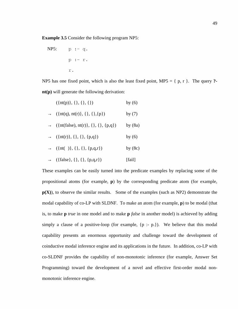
49

Example 3.5 Consider the following program NP5:

NP5: p :- q.

p :- r.

r.

NP5 has one fixed point, which is also the least fixed point, MP5 = { p, r }. The query ?-

nt(p) will generate the following derivation:

({nt(p)}, {}, {}, {}) by (6)

→ ({nt(q), nt(r)}, {}, {},{p}) by (7)

→ ({nt(false), nt(r)}, {}, {}, {p,q}) by (8a)

→ ({nt(r)}, {}, {}, {p,q}) by (6)

→ ({nt(����)}, {}, {}, {p,q,r}) by (8c)

→ ({false}, {}, {}, {p,q,r}) [fail]

These examples can be easily turned into the predicate examples by replacing some of the

propositional atoms (for example, p) by the corresponding predicate atom (for example,

p(X)), to observe the similar results. Some of the examples (such as NP2) demonstrate the

modal capability of co-LP with SLDNF. To make an atom (for example, p) to be modal (that

is, to make p true in one model and to make p false in another model) is achieved by adding

simply a clause of a positive-loop (for example, {p :- p.}). We believe that this modal

capability presents an enormous opportunity and challenge toward the development of

coinductive modal inference engine and its applications in the future. In addition, co-LP with

co-SLDNF provides the capability of non-monotonic inference (for example, Answer Set

Programming) toward the development of a novel and effective first-order modal non-

monotonic inference engine.

50

3.3 Declarative Semantics and Correctness Result

The declarative semantics of a co-inductive logic program with negation as failure (co-

SLDNF) is an extension of a stratified-interleaving (of coinductive and inductive predicates)

of the minimal Herbrand model and the maximal Herbrand model semantics with the

restriction of rational trees. This allows the universe of terms to contain rational (that is,

rationally infinite) terms, in addition to the traditional finite terms. As we noted earlier with

the program NP3 (in Example 3.2), the negation in logic program with coinduction may

generate nonmonotonicity and thus there exists no consistent co-Herbrand model. For a

declarative semantics to co-LP with negation as failure as failure, we rely on the work of

Fitting (1985) (Kripke-Kleene semantics with 3-valued logic), extended by Fages (1994) for

stable models with completion of a program. Their framework, which maintains a pair of

sets (corresponding to a partial interpretation of success set and failure set, resulting in a

partial model) provides a sound theoretical basis for the declarative semantics of co-SLDNF.

As we noted earlier, we restrict Fitting’s and Fages’s results within the scope of rational LP

over the rational space. We summarize this framework next.

Definition 3.5 (Pair-set and pair-mapping): Let P be a normal logic program, with its rational

Herbrand Space HSR(P), and let (M, N) ∈ 2HBx2HB (where HB is the rational Herbrand base

HBR(P)) be a partial interpretation. Then the pair-mapping (TP+, TP

-) for defining the pair-set

(M, N) are as follows:

TP+(M,N)={head(R) | R∈ HGR(P), pos(R) ⊆ M, neg(R) ⊆ N},

TP-(M,N) = {A | ∀R∈ HGR(P), head(R)=A → pos(R)∩N≠∅ ∨ neg(R)∩M≠∅}

where head(R) is the head atom of a clause R, pos(R) is the set of positive atoms in the body

of R, and neg(R) is the set of atoms under negation. �

51

It is noteworthy that the TP+ operator with respect to M of the pair set (M, N) is identical to

the immediate consequence operator TP (Lloyd, 1987) where TP(I) = { head(R) | R∈ HGR(P),

I |= body(R)} where body(R) is the set of positive and negative literals occurring in the body

of a clause R. We recall Lloyd (1987) and also noted by Fages (1994) that a Herbrand

interpretation I (that is, I ⊆ HG(P)) is a model of comp(P) iff I is a fixed point of Tp.

Intuitively, the outcome of the operator TP+ is to compute a success set. In contrast, the

outcome of TP- is to compute the set of atoms guaranteed to fail. Thus the pair-mapping

(TP+,TP

-) specifies essentially a consistent pair of a success set and a finite-failure set. Further

the pair-set (M, N) of the pair-mapping (TP+,TP

-) enjoys monotonicity and gives Herbrand

models (fixed points) under certain conditions as follows:

Theorem 3.1 (Fages 1994: Proposition 4.2, 4.3, 4.4, 4.5 and Theorem 4.6, 5.4, and Corollary

3.6): Let P be an infinite LP. Then:

(1) If M ∩ N = ∅ then TP+(M, N) ∩ TP

-(M, N) = ∅.

(2) < TP+, TP

-> is monotonic in the lattice 2HBx2HB (where HB is the Herbrand Base) ordered

by pair inclusion ⊆. That is, (M1, N1) ⊆ (M2, N2) implies that < TP+, TP

-> (M1, N1) ⊆

<TP+, TP

-> (M2, N2).

(3) If M ∩ N = ∅ and (M, N) ⊆ <TP+,TP

-> (M, N) then there exists a fixed point (M', N') of

<TP+, TP

- > such that (M, N) ⊆ (M', N') and M' ∩ N' = ∅.

(4) If (M, N) is a fixed point of <TP+, TP

->, M ∩ N=∅ and M ∪ N = HB, then M is a Herbrand

Model (HM) of comp(P).

(5) If an infinite logic program P is order-consistent then comp(P) has a Herbrand model.

(6) An order-consistent logic program has a stable model.

52

(7) If P is call-consistent and the relation ≤0 on predicate symbols is acyclic (where “p ≤0 q”

if there is a non-empty path from p to q with all edges positive), then P has a stable

model. �

Note that the pair mapping <TP

+, TP-> and the pair-set (M, N) are the declarative counterparts

of co-SLDNF resolution; the set (M, N) corresponds to (χ+, χ-) of Definition 3.5. Fages’s

theorem above captures the declarative semantics of co-SLDNF resolution for general

infinite LP. The proofs for Theorem 3.1 (1-2) are straightforward. For Theorem 3.1 (3) with

HGR(P), the immediate consequence (of the pair-set (M, N) by the pair-mapping <TP+, TP

->

applied each time) is rational, and this is true for any finite n steps where n ≥ 0. This is due

to the earlier observations: (i) that the algebra of rational trees and the algebra of infinite trees

are elementarily equivalent, (ii) that there is no isolated irrational atom as result of the pair-

mapping and pair-set for rational LP over rational space, and (iii) that any irrational atom as

result of an infinite derivation in this context should have a rational cover, as noted in Jaffar

and Stuckey (1986), which could be characterized by the (interim) rational atom observed in

each step of the derivation. For Theorem 3.1 (4), there are two cases to consider for each

atom resulting in a fixed point: rational and irrational. For the rational case, it is

straightforward that it will be eventually derived by the pair-mapping as there is a rational

cover that eventually converges to the rational atom, and the rational model contains the

fixed point. For the irrational case, the fixed point does not exist in the program’s rational

space but there is a rational cover converging into the irrational fixed point over infinity. That

is, there is a fixed point but its irrational atom is not in the rational model. In this case, co-

SLDNF derivation (tree) will be irrational, to be labeled undefined. The proof for Theorem

3.1 (5) for a finite LP is straightforward, and for Theorem 3.1 (6) and (7) for a finite LP.

53

Note that an order-consistent program is essentially without any cycle when it is grounded.

Fages further noted that the premises of (7) to be decidable even for infinite LP, which

provides a justification for the preprocessing to check for the call-consistency with predicate

dependency graph as we elaborate in Chapter 4. Moreover the acyclic requirement for “p ≤0

q” (for a non-empty path from p to q with all edges positive) can be checked easily with a

very minor enhancement to co-SLDNF derivation and its trace of successful subgoals in the

path. This acyclic requirement is also the thesis of Lin and Zhao (2002) for a formal proof

and its application to Boolean SAT solver to solve ASP. Further, we can establish that a

model of P with respect to a successful co-SLDNF derivation is also a model of comp(P), to

show that a program P and its completion comp(P) coincide under a successful co-SLDNF

resolution. As we noted earlier, the pair mapping <TP+, TP

-> and the pair-set (M, N) are the

declarative counterparts of co-SLDNF resolution where the set (M, N) corresponds to (χ+, χ-

) of Definition 3.3.

Corollary 3.2 (Fages’s Theorem for Rational Models): Let P be a normal coinductive logic

program. Let (TP+, TP

-) be the corresponding pair mappings [Def. 3.5]. Given a pair set (M,

N) ∈ 2HBx2HB [where HB is the rational Herbrand base HBR(P)] with M∩N = ∅ and (M, N)

⊆ < TP+, TP

- >(M, N) then there exists a fixed point (M', N') of < TP+,TP

- > such that (M, N) ⊆

(M', N') and M' ∩ N' = ∅. If (M', N') is a fixed point of < TP+,TP

->, M' ∩ N' = ∅ and M' ∪ N'

= HBR(P), then M’ is a (Rational) Herbrand model of P (denoted HMR(P)). �

Note that there may be more than one fixed points which are possibly inconsistent with each

other. As we show later, HMR(P) is a model of comp(P) since comp(P) coincides with P

under co-SLDNF. As noted earlier, the condition of mutual exclusion (that is, M∩N = ∅)

54

keeps the pair-set (M,N) monotonic and consistent under the pair-mapping. The pair-

mapping with the pair-set maintains the consistency of truth value assigned to an atom p.

Thus, the cases where both p and not p are assigned true, or both are assigned false, are

rejected. Next we show that P coincides with comp(P) under co-SLDNF. We recall the

work of Apt, Blair and Walker (1988) for supported interpretation and supported model.

Definition 3.6 (Supported Interpretation (Apt, Blair, and Walker 1988). An interpretation I of

a general program P is supported if for each A∈I there exists a clause A1←L1,...,Ln in P and a

substitution θ such that I |= L1θ, ..., Lnθ, A=A1θ, and each Liθ is ground. Thus I is supported

iff for each A∈I there exists a clause in HG(P) with head A whose body is true in I. �

Theorem 3.3 (Apt, Blair, and Walker 1988; Shepherdson 1988). Let P be a general

program. Then:

(1) I is a model of P iff TP(I) ⊆ I.

(2) I is supported iff TP(I) ⊇ I.

(3) I is a supported model of P iff it is a fixed point of TP, that is, TP(I) = I. �

We use these results to show that comp(P) and P coincide under co-SLDNF resolution. The

positive and negative coinductive hypothesis tables (χ+ and χ-) of co-SLDNF are equivalent

to the pair-set under the pair-mapping and thus enjoy (a) monotonicity, (b) mutual exclusion

(disjoint), (c) consistency. First (1), it is straightforward to see that in a successful

co-SLDNF derivation the coinductive hypothesis tables χ+ and χ- serve as a partial model.

That is, if the body of a selected clause is true in χ+ and χ- then its head is also true (A ←

L1,...,Ln). Second (2), it is also straightforward to see that a successful co-SLDNF derivation

55

constrains the coinductive hypothesis tables χ+ and χ- at each step to stay supported. That is,

if the head is true then the body of the clause is true (that is, A → L1,...,Ln). By co-inductive

hypothesis rule, the selected query subgoal (say, A) is placed first in χ+ (resp. χ-) depending

on its positive (resp. negative) context. The rest of the derivation is to find a right selection

of clauses (A → L1,...,Ln) whose head-atom is unifiable with A, and whose body is true using

normal logic programming expansion or via negative or positive coinduction hypothesis rule.

Thus it follows from above that a coinductive logic program (A ← L1,...,Ln) is equivalent to

its completed program (A ↔ L1,...,Ln) under co-SLDNF resolution.

Correctness of co-SLDNF resolution is proved by equating the operational and

declarative semantics via the soundness and completeness theorems, restricted to rational

Herbrand Space. The restriction to the rational Herbrand space (of terms, atoms, and trees of

atoms) for the operational semantics is guaranteed to terminate finitely. We now state the

soundness and completeness theorems for co-SLDNF.

Theorem 3.4 (Soundness and Completeness of co-SLDNF). Let P be a general program over

its rational Herbrand Space.

(1) (Soundness of co-SLDNF): (a) If a goal {A} has a successful derivation in program P

with co-SLDNF, then A is true (that is, there is a model HMR(P) such that A ∈ HMR(P)). (b)

If a goal { nt(A) } has a successful derivation in program P, then nt(A) is true (that is, there is

a model HMR(P) such that A ∈ HBR(P)\HMR(P)).

(2) (Completeness of co-SLDNF): (a) If there is a model HMR(P) such that A ∈ HMR(P),

then A has a successful co-SLDNF derivation or an irrational derivation. (b) If there is a

56

model HMR(P) such that A ∈ HBR(P)\HMR(P), then nt(A) has a successful co-SLDNF

derivation or an irrational derivation. �

Proof. We first prove the case when A (or nt(A)) has a coinductive proof (that is, the fairness

assumption), and then the alternative proof for soundness, then for the case of irrational

derivation for completeness. It is straightforward from Definition 3.5 and Theorem 3.1

(Fages, 1994) and Definition 3.6 and Theorem 3.3 (Apt, Blair, and Walker 1988). The basic

idea of the proof is to show that, given a program P and a query goal A (a list of one or more

positive or negative literals), a successful co-SLDNF derivation with its coinductive

hypothesis tables of (χ+, χ-) at each step is essentially equivalent to (1) the partial

interpretation with the pair-mapping <TP+, TP

-> and the pair-set (M, N) (by Theorem 3.1,

resulting in a fixed point), where (2) (χ+, χ-) is to be kept closed (a model) and supported (by

Theorem 3.3). We show that the hypothesis tables (χ+, χ-) of a successful co-SLDNF

derivation is (1) monotonic, mutually exclusive (disjoint), and consistent and it is (2) a model

(or closed) and supported (of Definition 3.6 and Theorem 3.3).

First (1), a successful co-SLDNF derivation maintains the coinductive hypothesis

tables χ+ and χ- at each step of derivation. These two tables are monotonic, consistent and

mutually-exclusive along a single co-SLDNF derivation. They are monotonic because co-

SLDNF only adds to the tables χ+ and χ- in each derivation step. They are consistent and

mutually exclusive because if an inconsistency is created, backtracking will take place.

Second (2), it is straightforward to see that a successful co-SLDNF derivation

enforces the coinductive hypothesis tables χ+ and χ- at each step to be a model. That is, if

the body of a selected clause is true then its head is true (that is, A ← L1,...,Ln) due to the use

57

of co-inductive hypothesis rule (that is, TP↓, as in Lloyd (1987), the Knaster-Tarski

immediate-consequence one-step operator TP) as well as normal resolution.

Third (3), it is straightforward to see that a successful co-SLDNF derivation enforces

the coinductive hypothesis tables χ+ and χ- at each step to be supported. That is, if the head

is true then the body of the clause is true (that is, A → L1,...,Ln). By co-inductive hypothesis

rule, the selected query subgoal (say, A) is placed first in χ+ (or χ-, resp.) depending on its

positive (or negative context, resp.); The rest of the derivation is to find a right selection of

clauses (A → L1,...,Ln) whose head-atom is unifiable with A, and whose body is true using

normal logic programming expansion resulting in resolution with a unit clause or via

coinduction (that is, the goal is found in χ+ if it occurs in a positive context, or the goal is

found in χ- if it occurs in a negative context). Further it follows from (2) (A ← L1,...,Ln) and

(3) (A → L1,...,Ln) above that a co-inductive LP is equivalent to its completed program (A ↔

L1,...,Ln) under co-SLDNF.

Thus, co-SLDNF generates a successful derivation (that is, co-SLDNF refutation)

given an arbitrary query goal A in HBR iff A is in a supported model iff A is in a fixed point

of P iff A is in HMR(P), as we restrict current proof to the rational Herbrand model. In

summary, we note four points as a conclusion. First (1), (for soundness) if there is a

successful co-SLDNF derivation of a goal A in HMR(P), then P |= A (or A is of a fixed point

of P). Second (2), (for completeness) if P |= A in HMR(P) then there is a successful

co-SLDNF derivation, and further for a query goal in negative context (for example, nt(A)).

Third (3), (for soundness) if there is a successful co-SLDNF derivation of a goal nt(A), then

P |= ¬A (that is, A is in HBR(P)\HMR(P)) or A is not in a fixed point of P). Finally (4), (for

completeness) if P |= ¬A (that is, A is in HBR(P)\HMR(P)), then there is a successful

58

co-SLDNF derivation for nt(A). Further the generalization of the theorem for a normal query

goal of a list of positive and negative literals can be derived in a straightforward manner (for

example, by using a single atom to be expanded into a clause of the query goal-list). �

This completes the soundness and completeness of co-SLDNF resolution. There are two

points to note. First (1), as we noted in the proof, a co-inductive logic program is equivalent

to its completion of program under co-SLDNF. Second (2), there is no need for the

restriction on stratification (that is, the stratification of coinductive predicates with respect to

negation) and ranking of negation as failure in co-SLDNF completeness proof, contrast to

the proof of SLDNF completeness. As we noted earlier, there are two ways to prove the

equivalence: to show P coincides with comp(P), and then by Theorem 3.1 (4), and to show I

= (M, N) is a supported model of P, and then using Theorem 3.3 (3).

For the benefit of those who are familiar with the classical SLDNF proofs, we

provide an alternative proof of the soundness of co-SLDNF derivation (Theorem 3.4 (1))

below based on induction on the length of the derivation, to show that P |= A (or P |= ¬A,

resp.) if there is a successful co-SLDNF derivation of the query goal A (or nt(A), resp.). Since

we restrict negated goals to be grounded, we assume that given a query goal A (or nt(A),

resp.), then A is a ground atom.

Alternative Proof of Soundness (Theorem 3.4 (1)): Given a program P and an atomic

query goal A where A occurs in a positive context (resp. nt(A), where goal A occurs in a

negative context), let there be a successful co-SLDNF derivation of length n starting with

(G0, E0, χ0+, χ0-) = ({A}, {}, {}, {}) as the initial state of the derivation.

(1) Base case: n = 1 for G0={A} (n = 1 for G0={nt(A)}).

59

(1.a) For query goal G0={A} there is a successful co-SLDNF derivation with a unit clause

whose head-atom unifies with A using Definition 3.3 step 5; otherwise, there is no successful

co-SLDNF derivation of length 1 for an atom A in positive context). Let the selected clause

be C1: A1 ←, with an empty body, and θ1 = mgu(A, A1).

(5) C1,θ1 ({ A},{},{},{}) → (����, θ1, {A}, {}) [success]

Note that the only way in which subgoal A in positive context can succeed in one-derivation-

step is (i) by coinductive hypothesis rule where A unifies with A' in χ+ (Definition 3.3 step

1), or (ii) by a unit clause where A unifies with A' (the head-atom of the unit clause)

(Definition 3.3 step 5).

(1.b) For a query goal G0={ nt(A) }, for a ground atom A in negative context, there is a

successful co-SLDNF derivation (i) only if there is no clause whose head unifies with A

(using Definition 3.3 step 6):

(6) (8)(a) ({ nt(A)}, ∅, ∅, ∅) → ((nt(false),{},{},{ A}) → ((����,{},{},{A}) [success]

Or, (ii) it can succeed in one derivation step is either by the coinductive hypothesis rule

where A unifies with A' in χ- (Definition 3.3 step 6 and then step 2; for example, with a rule {

A ← A. }):

(6) (2), (8)(b) ({ nt(A)}, ∅, ∅, ∅) → ((nt(A),{},{},{ A}) → ((����,{},{},{ A}) [success]

In (1.a), since a successful derivation is achieved in one step either due to the goal matching

a fact or due to the goal being present in χ+ (that is, due to a rule of the form A :- A.), it is

easy to see that in such a case, A will be present in the gfp of the program P, that is, P |= A.

Similar reasoning can be performed for (1.b) that a successful derivation is achieved in two

steps either due to the goal matching no fact or due to the goal being present in χ- (that is,

60

due to a rule of the form A :- A.) and that there is no successful co-SLDNF derivation for the

goal A. It is easy to see that in such a case, A will be not in a fixed point of the program P

(that is, P |= ¬A). Therefore, (1) P |= A iff A ∈ MR(P), and (2) P |= ¬A iff A ∈

HBR(P)\HMR(P).

(2) Inductive case: Let us assume that the inductive hypothesis holds for n - 1.

(2.1) (case for n > 1, with atom A in positive context): Let query goal G0={A} (a ground atom

A in positive context) for program P. Let A be expanded initially with a clause C which is

arbitrarily chosen in P, where C: A' ←B1, ..., Bm, and θ=mgu(A, A'). Then:

(5) C,θ D: ({A},{},{},{}) → ({B1θ, ..., Bmθ}, { θ}, { A},{})

Assume, by induction hypothesis, ({B1θ, ..., Bmθ}, { θ}, { A},{}) has a successful co-SLDNF

derivation of length n - 1 (let D1 denote this successful co-SLDNF derivation) then P |= B1θ,

..., Bmθ.

(2.1.a) A is not in a cycle in D1, then there is no application of step 1 of Definition 3.3 with A

in the positive coinductive hypothesis table, in D1. Then D will have a successful co-SLDNF

derivation of length of n. Since P |= B1θ, ..., Bmθ and A' ← B1,...,Bm, therefore P |=A'θ which

implies P |= A, and the lemma holds for this case.

(2.1.b) A will form a cycle in D1: In such a case, there should be a derivation step where a

subgoal A' unifies with A and coinductively succeeds with A in the positive hypothesis table

at that point (Definition 3.3 step 1). With respect to the declarative semantics, we are only

interested in fixpoints that contain A. It is easy to see that A succeeds in n steps, since A is

present in the positive coinductive hypothesis table. Note that for all the fixpoints that

contain A, ({B1θ, ..., Biθ, ... Bmθ}, {}, {}, {}) will have a successful co-SLDNF derivation,

61

since Biθ will eventually reach A, which will reach Biθ again, and coinductively succeed at

that point). Since P |= B1θ, ..., Bmθ, and A' ←B1, ..., Bm again, A'θ will become part of a fixed

point, implying P |= A'θ, in turn implying P |= A, and the lemma holds for this case.

(2.2) (case for n > 1, with a ground atom A in negative context): Let query goal G0={nt(A)}

(for example, a ground atom A in negative context) for program P. Let A be expanded

initially with a clause C which is arbitrarily chosen in P, where C: A' ← B1,...,Bm, and θ =

mgu(A, A'). Then:

(5) C,θ D: ({nt(A)},{},{},{}) → ({nt(B1θ, ..., Bmθ)}, { θ}, {},{ A})

If there is no such clause C, then this case is covered in (1.b) above. Therefore let us assume

by induction hypothesis that ({nt(B1θ, ..., Bmθ)}, { θ}, {},{ A}) has a successful co-SLDNF

derivation of length n - 1, and D1 denotes this successful co-SLDNF derivation. By

induction hypothesis there is at least one Biθ such that P |= ¬Biθ.

By step 8(a) in Definition 3.3, let Biθ (1 ≤ i ≤ m) be reduced to false (as shown

below, and further without loss of generality, let Biθ be the only such one so that there is no

successful co-SLDNF derivation from ({B1θ, ..., Biθ, ... Bmθ}, { θ}, {},{ A}):

D1: ({nt(B1θ, ..., Biθ, ... Bmθ)}, { θ}, {},{ A}) → ...

→ ({nt(B1θ, ..., false, ... Bmθ)}, {...}, {...},{ A, ...})

(8)(a) → ((����,{...},{...},{ A, ...}) [success]

There are several subcases to consider:

(2.2.a) A in negative context is not in cycle in D1, then there is no application of step 2 of

Definition 3.3 with A in the negative coinductive hypothesis table, in D1. That is, ({nt(B1θ,

62

..., Bmθ)}, {}, {}, {}) has a successful co-SLDNF derivation. Let n - 1 be the length of D1.

Then D will have a successful co-SLDNF derivation of length of n. Clearly, since P |= ¬Biθ,

it follows that P |= ¬A'θ; thus, P |= ¬A.

(2.2 b) A in negative context in a cycle with A' in D1. For a successful co-SLDNF

derivation, A' must be in a negative context also. Without loss of generality, assume that at

least one of Bkθ occurs in a positive context and one Biθ that occurs in a negative context.

Since there may be multiple fixpoints, for nt(A) we are interested in only those fixpoints

which do not contain A. By induction hypothesis at least one of these fixpoints will contain

all such Bkθ’s and will not contain all such Biθ’s. Thus, all Bkθ and nt(Biθ) goals will have a

successful derivation. Since A is in a cycle, one of the Bkθ or Biθ will end up placing A'θ in

χ-. Therefore it is now straightforward to see that that if nt(A) has a successful co-SLDNF

derivation then P |= nt(A).

We have shown that by inductive hypothesis, if ({B1θ, ..., Bmθ}, { θ}, { A}, {}) (resp.

({ nt(B1θ, ..., Bmθ)}, { θ}, {}, { A})) has a successful co-SLDNF derivation in P, then P |= B1θ,

..., Bmθ (resp. P |= ¬(B1θ, ..., Bmθ)). Further, A (resp. nt(A)) is expanded initially with a

clause C which is arbitrarily chosen in P [by Definition 3.3 step 5] (resp. with all such clause

C [by Definition 3.3 step 6]), where C: A' ←B1, ..., Bm, and θ = mgu(A, A'). Therefore, by

induction hypothesis, if there is a successful co-SLDNF derivation for query goal {A} (or

{ nt(A)}, resp.) then P |= A (or P |= ¬A, respectively). That is, P |= A iff A∈ HMR(P), and P

|= ¬A iff A∈ HBR(P)\HMR(P). This concludes the alternative proof of soundness of co-

SLDNF. �

63

Note that the coincidence of P and comp(P) under co-SLDNF is important. As we

noted earlier, a coinductive logic program (A ← L1,...,Ln) is equivalent to its completed

program (A ↔ L1,...,Ln) under co-SLDNF resolution. Thus we have the following corollary.

Corollary 3.5 (Equivalence of P and comp(P)): Let P be a normal co-LP, with a successful

co-SLDNF derivation for atom A in P. Then: P |= A iff comp(P) |= A. �

If comp(P) is not consistent, say with respect to an atom p, then there is no successful (finite

or rational) derivation of p or nt(p). For a finite derivation, we noted earlier with the

program NP3 = { p :- nt(p). } in Example 3.2. For an infinite derivation, let us elaborate with

the following example.

Example 3.6 Let us consider the following program IP1:

IP1: q :- p(a).

p(X) :- p(f(X)).

The derivation for query ?- q (that is, q → p(a) → p(f(a)) → p(f(f(a))) → ...) is non-

terminating. This is an example of an irrational derivation (irrational proof tree). Similarly

the negated query ?- nt(q) is also non-terminating (that is, nt(q) → nt(p(a)) → nt(p(f(a))) →

nt(p(f(f(a)))) → ... ). But it is clear that both q and p(a) are in the Herbrand base, HBR(P),

of P. For the second clause { p(X) :- p(f(X)). }, there is only one ground (rational) atom

p(X') where X' = f(X ') = f(f(f(...))) . The atom p(X') satisfies the clause and makes p(X) true.

All other finite or rational atoms other than p(X') are undefined because each as a query goal

will have an irrational derivation. Granted an irrational derivation, q and p(a) will have a

successful irrational derivation to be true, that is, in HM(P). The ground atom p(f(f(f(...)))) is

in HMR(P). All other finite and rational atoms p(Y) in HBR(P) where Y ≠ f(Y) are

64

undefined even though they should be in HMR(P) as one would expect. The derivation of

query ?- q which is irrational hence will not terminate. If there is no finite or rational

coinductive proof for an atom G, then the query G will have an irrational infinite derivation

even though we cannot tell whether G is true or false. Let us consider the second example of

the program IP2 as follows:

IP2: q :- nt(p(a)).

p(X) :- p(f(X)).

Similar to the program IP1, it is clear that both q and p(a) are in the Herbrand base, HBR(P),

of P. Moreover, q is in HMR(P), p(a) is in HBR(P)/HMR(P), and p(Y) is in HMR(P) if Y ≠ a.

The only atom with a successful (rational) derivation is p(Z) where Z = f(Z) .

3.4 Implementation

The implementation of co-SLDNF resolution on top of Prolog engine is presented in this

section. We have two versions of the implementation for the co-SLDNF interpreter. The

first implementation is done on top of YAP Prolog1 (Bansal, 2008) shown in Table 3.1. This

version has been used primarily for the test platform for co-LP programs and for the base

platform for ASP Solver. Note that here we use two distinct notations for the coinductive

negation, as the negation as failure (naf) of co-LP, for this implementation: one for the head

and the other for the body. When an atom is negated for the head, we use nt/1. For example,

a negated atom (for example, for B) in the head would be nt(B). When an atom is negated

for the body, we use nnot/1 (for example, nnot(B)). Further we may distinguish the

1 http://www.dcc.fc.up.pt/~vsc/Yap/

65

coinductive negation (nt/1 or nnot/1) from the inductive negation (not/1) for the negation

operator in Prolog.

Table 3.1. Implementation of co-SLDNF atop YAP

:- dynamic coinductive/4. init_coinductive_vars :- nb_setval(positive_hypo, [ ]), nb_setval(negative_hypo, []). :- init_coinductive_vars. coinductive(F/N) :- atom_concat(coinductive_,F,NF), functor(S,F,N), functor(NS,NF,N), match_args(N,S,NS), atom_concat(stack_,F,SFn), atomic_concat(SFn,N,SF ), atom_concat(SF, '_posHypo', SFpos), nb_setval(SFp os, []), atom_concat(SF, '_negHypo', SFneg), nb_setval(SFn eg, []), assert((S :- b_getval(SFpos,PSL), (in_stack(S,PSL), !, my_succ; b_getval(SFneg,NSL), in_stack(S,NSL), !, m y_fail; b_setval(SFpos,[S|PSL]), b_getval(positive_hypo, GPSL), b_setval(positive_hypo,[S|GPSL]), NS) )), assert((nnot(S) :- b_getval(SFneg,NSL), (in_stack(S,NSL), !, my_succ; b_getval(SFpos,PSL), in_stack(S,PSL), !, my_fail; b_setval(SFneg,[S|NSL]), b_getval(negative_hypo, GNSL), b_setval(negative_hypo,[S|GNSL]), (clause(nt(S),_) -> nt(S); nt_succ)) )), assert(coinductive(S,F,N,NS)). %-------------------------------------------------- --- match_args(0,_,_) :- !. match_args(I,S1,S2) :- arg(I,S1,A), arg(I,S2,A), I1 is I-1, match_args(I1,S1, S2). my_succ. nt_succ. my_fail :- fail. %-------------------------------------------------- --- term_expansion((H:-B),(NH:-B)):-coinductive(H,_F,_N ,NH), !. term_expansion(H,NH) :- coinductive(H,_F,_N,NH), !. %-------------------------------------------------- --- in_stack(G,[G|_]) :- !. in_stack(G,[_|T]) :- in_stack(G,T). not_in_stack(_G,[]). not_in_stack(G,[H|T]) :- G \== H, not_in_stack(G,T) .

66

Next, we present the second version of the co-SLDNF interpreter, listed in Table 3.2. This

implementation is the extension of the original co-SLD metainterpreter implemented by

Simon (2006) by adding the negation as failure for co-LP. This is initially built atop of

Sicstus Prolog2, and is adapted also run atop of SWI Prolog3 which is used primarily for the

programs with greatest or maximal fixed point semantics. Here nt/1 is used consistently for

negative literal occurring in the head and the body.

Table 3.2. Implementation of co-SLDNF on top of co-SLD

/************************************* ===================================== CO-LOGIC PROGRAMMING META-INTERPRETER ===================================== Luke Simon - June 16, 2006 Richard K. Min - March 20, 2008 USAGE ----- Include this file in your co-LP source file. All us er defined predicates must be declared dynamic due to a limitation in the clause/2 predicate, and user pred icate definitions and queries can only make use of user d efined predicates or the list of built in predicates below . Note that it is forbidden to redefine a built in predica te. A query is executed by loading the co-LP source fil e as usual. Then queries must begin and end, respective ly, with "query((" and "))." in order to be executed with alternating SLD and co-SLD semantics using a coindu ctive hypothesis first, left-most, depth-first search str ategy. query( Goal ). solve( Hypothesis, Goal ). Hypothesis has type atom-list. Goal has type goal.

2 http://www.sics.se/isl/sicstuswww/site/index.html

3 http://www.swi-prolog.org/

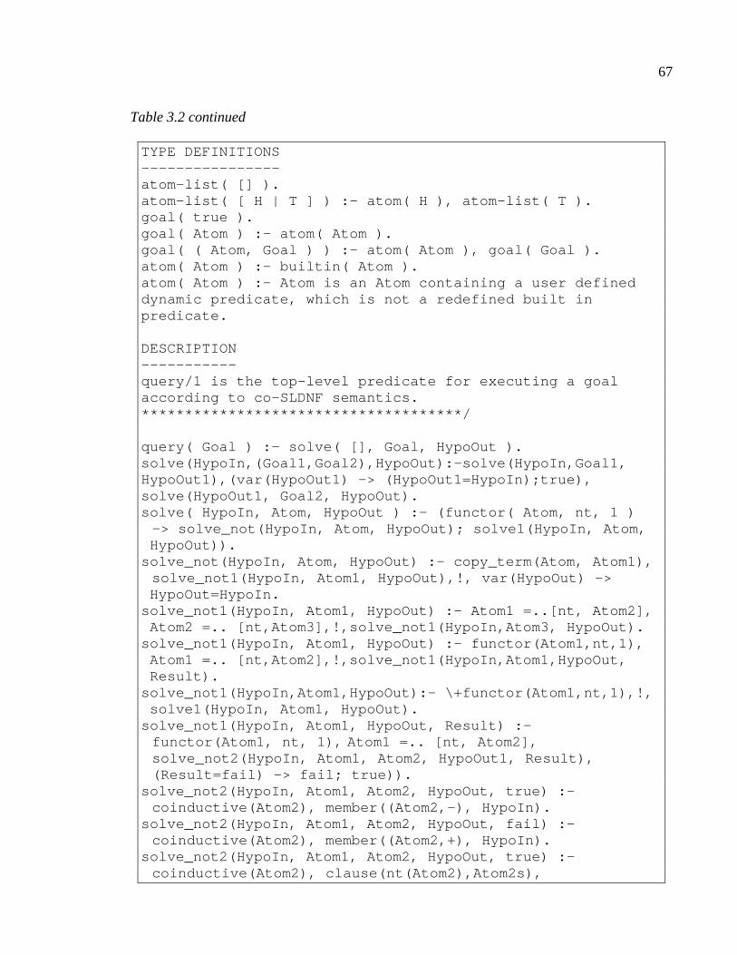
67

Table 3.2 continued

TYPE DEFINITIONS ---------------- atom-list( [] ). atom-list( [ H | T ] ) :- atom( H ), atom-list( T ) . goal( true ). goal( Atom ) :- atom( Atom ). goal( ( Atom, Goal ) ) :- atom( Atom ), goal( Goal ). atom( Atom ) :- builtin( Atom ). atom( Atom ) :- Atom is an Atom containing a user d efined dynamic predicate, which is not a redefined built i n predicate. DESCRIPTION ----------- query/1 is the top-level predicate for executing a goal according to co-SLDNF semantics. *************************************/ query( Goal ) :- solve( [], Goal, HypoOut ). solve(HypoIn,(Goal1,Goal2),HypoOut):-solve(HypoIn,G oal1, HypoOut1),(var(HypoOut1) -> (HypoOut1=HypoIn);true) , solve(HypoOut1, Goal2, HypoOut). solve( HypoIn, Atom, HypoOut ) :- (functor( Atom, n t, 1 ) -> solve_not(HypoIn, Atom, HypoOut); solve1(HypoIn , Atom, HypoOut)). solve_not(HypoIn, Atom, HypoOut) :- copy_term(Atom, Atom1), solve_not1(HypoIn, Atom1, HypoOut),!, var(HypoOut) -> HypoOut=HypoIn. solve_not1(HypoIn, Atom1, HypoOut) :- Atom1 =..[nt, Atom2], Atom2 =.. [nt,Atom3],!,solve_not1(HypoIn,Atom3, Hy poOut). solve_not1(HypoIn, Atom1, HypoOut) :- functor(Atom1 ,nt,1), Atom1 =.. [nt,Atom2],!,solve_not1(HypoIn,Atom1,Hyp oOut, Result). solve_not1(HypoIn,Atom1,HypoOut):- \+functor(Atom1, nt,1),!, solve1(HypoIn, Atom1, HypoOut). solve_not1(HypoIn, Atom1, HypoOut, Result) :- functor(Atom1, nt, 1), Atom1 =.. [nt, Atom2], solve_not2(HypoIn, Atom1, Atom2, HypoOut1, Result) , (Result=fail) -> fail; true)). solve_not2(HypoIn, Atom1, Atom2, HypoOut, true) :- coinductive(Atom2), member((Atom2,-), HypoIn). solve_not2(HypoIn, Atom1, Atom2, HypoOut, fail) :- coinductive(Atom2), member((Atom2,+), HypoIn). solve_not2(HypoIn, Atom1, Atom2, HypoOut, true) :- coinductive(Atom2), clause(nt(Atom2),Atom2s),

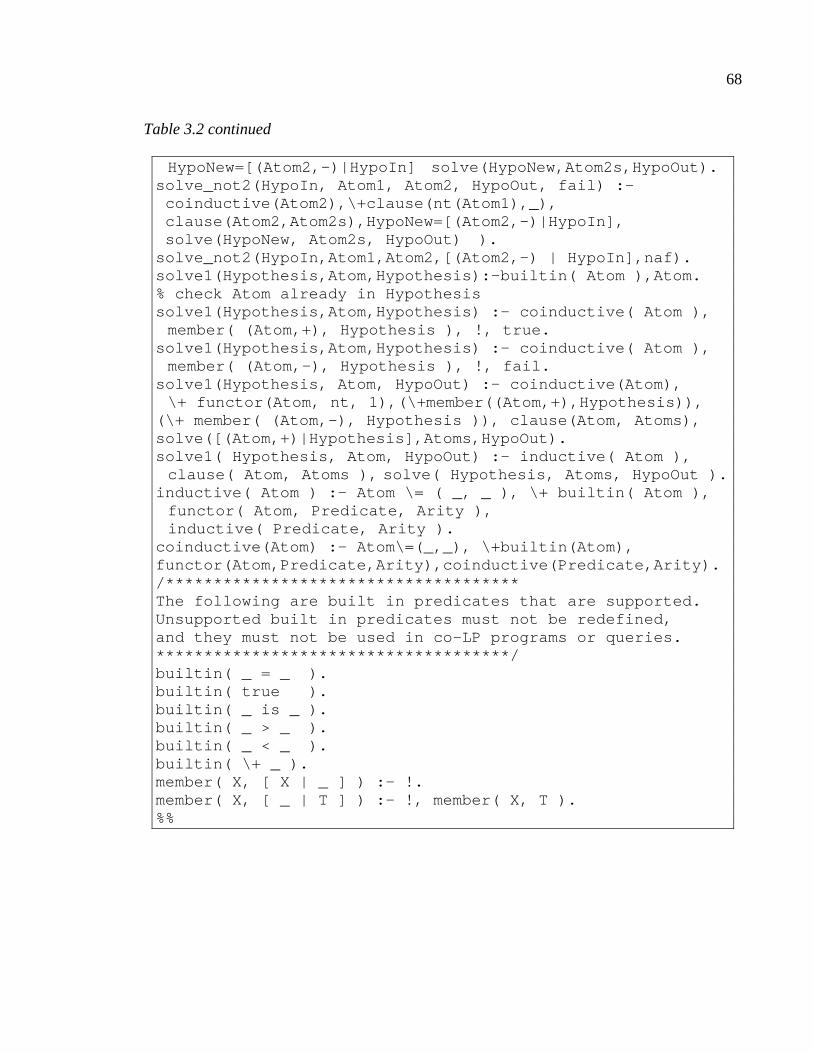
68

Table 3.2 continued

HypoNew=[(Atom2,-)|HypoIn] solve(HypoNew,Atom2s,Hy poOut). solve_not2(HypoIn, Atom1, Atom2, HypoOut, fail) :- coinductive(Atom2),\+clause(nt(Atom1),_), clause(Atom2,Atom2s),HypoNew=[(Atom2,-)|HypoIn], solve(HypoNew, Atom2s, HypoOut) ). solve_not2(HypoIn,Atom1,Atom2,[(Atom2,-) | HypoIn], naf). solve1(Hypothesis,Atom,Hypothesis):-builtin( Atom ) ,Atom. % check Atom already in Hypothesis solve1(Hypothesis,Atom,Hypothesis) :- coinductive( Atom ), member( (Atom,+), Hypothesis ), !, true. solve1(Hypothesis,Atom,Hypothesis) :- coinductive( Atom ), member( (Atom,-), Hypothesis ), !, fail. solve1(Hypothesis, Atom, HypoOut) :- coinductive(At om), \+ functor(Atom, nt, 1),(\+member((Atom,+),Hypothe sis)), (\+ member( (Atom,-), Hypothesis )), clause(Atom, A toms), solve([(Atom,+)|Hypothesis],Atoms,HypoOut). solve1( Hypothesis, Atom, HypoOut) :- inductive( At om ), clause( Atom, Atoms ), solve( Hypothesis, Atoms, H ypoOut ). inductive( Atom ) :- Atom \= ( _, _ ), \+ builtin( Atom ), functor( Atom, Predicate, Arity ), inductive( Predicate, Arity ). coinductive(Atom) :- Atom\=(_,_), \+builtin(Atom), functor(Atom,Predicate,Arity),coinductive(Predicate ,Arity). /************************************* The following are built in predicates that are supp orted. Unsupported built in predicates must not be redefin ed, and they must not be used in co-LP programs or quer ies. *************************************/ builtin( _ = _ ). builtin( true ). builtin( _ is _ ). builtin( _ > _ ). builtin( _ < _ ). builtin( \+ _ ). member( X, [ X | _ ] ) :- !. member( X, [ _ | T ] ) :- !, member( X, T ). %%

69

CHAPTER 4

COINDUCTIVE ANSWER SET PROGRAMMING

4.1 Introduction

As we noted earlier in Chapter 3, one striking observation is that P and P* are equivalent

with respect to co-SLDNF. That is, P |= A iff comp(P) |= A, under a successful co-SLDNF

derivation. This ground-breaking result leads us initially to believe that co-SLDNF

resolution can be a building block in obtaining goal-directed implementation of answer set

programs which many thought to be impossible. This is indeed consistent with many results

concerning comp(P), stable model of comp(P) and ASP, as noted in Fages (1994), and

further it provides a compatible semantics required for ASP solver with co-LP. Current

work is an extension of our previous work discussed for grounded (propositional) ASP

Solver (Gupta et al. 2007).

4.2 ASP Solution Strategy

To solve ASP program in general case (that is, toward predicate ASP) is essentially to

overcome the three-fold restrictions imposed upon current ASP as we noted in Chapter 2.

That is, (a) positive-loop free (for example, not allowing a rule such as { p :- p. }), (b)

range-restricted, and (c) function-free ASP. Overcoming these restrictions, we plan to

achieve the following objectives, which will be elaborated later in this Chapter. First (1), it

is to eliminate the preprocessing requirement of grounding, directly processing the

predicates with variables and function symbols. Second (2), it is therefore to extend current

70

ASP language to be truly predicate normal logic programming language with variables and

function symbols without any restriction. Third (3), further it is not only to provide stable

model semantics with least fixed point (lfp) but also to extend its capability to provide

partial models with maximal fixed point (mfp) or greatest fixed point (gfp) (to provide an

effective and alternative solution even to an incomplete or inconsistent but very-large

KnowledgeBase). Fourth (4), it is to handle vicious cycles and constraint rules effectively

and logically with negation. And finally (5), it is to demonstrate an alternative paradigm of

ASP solver and solution strategy, radically different from current ASP solvers, being top-

down, goal-directed and query-oriented, in addition to provide alternative partial model and

to model infinite objects and processes.

We achieve this novel and elegant ASP solver by coinductive logic programming

(Co-LP) with coinductive SLDNF (co-SLDNF) resolution as a viable and attractive

alternative to (a) current theoretical foundation and its implementation of current ASP

solvers and (b) its language extension to first order logic with function symbols and rational

(infinite) normal logic programming. We term this ASP with co-LP as coinductive Answer

Set Programming (co-ASP), and this ASP solver with co-LP as coinductive ASP Solver (co-

ASP Solver). The (extended) co-ASP language (syntax and semantics) is that of the basic

ASP language syntax (excluding the extended features such as weight, cardinality or choice

rule, etc.) with its stable semantics, of normal logic programming with function symbols and

cycles restricted with the rational domain of rational terms, atoms, and trees. However,

current scope of co-ASP excludes the irrational solutions and the general disjunctive logic

programs, but allows its syntax to construct infinite rational terms and atoms, and to have

positive-loop cycle (for example, { p :- p. }). The solution-strategy of co-ASP Solver is first

71

to transform ASP program into coinductive ASP (co-ASP) program and by following the

solution-strategy as follows: (1) to find a partial model (solution) with co-SLDNF, (2) to

eliminate positive-loop (gfp) solution (for example, “p” for { p :- p. }, thus to be minimal),

(3) to handle constraint rules and its integrity check (with a preprocessing and the completed

definition of program as needed), and (4) to check for a total model (with a preprocessing

and a post-processing). We note that at this early stage of co-ASP Solver with its prototype

we claim an achievement to demonstrate co-ASP Solver with a modest performance.

Current prototype implementation is too premature in performance and benchmark to be

compared with current mainstream ASP solvers, SAT solvers, or Constraint Logic

Programming in solving a practical problem.

However, the prospective of co-ASP Solver even at this stage is very promising as a

milestone and ground-breaking achievement in ASP and co-LP. Our approach possesses the

following advantages. First (1), it works with answer set programs containing first order

predicates with no restrictions placed on them. Second (2), it eliminates the preprocessing

requirement of grounding so that the predicates are executed directly in the manner of

Prolog. Our method constitutes a top-down/goal-directed/query-oriented paradigm for

executing answer set programs, a radically different alternative to current ASP solvers. We

term ASP solver realized via co-induction as coinductive ASP Solver (co-ASP Solver).

4.3 Transforming an ASP Program

First task toward solving ASP program with co-LP is to make an ASP program compatible

with the syntax of co-LP with co-SLDNF resolution. The task of transforming an ASP

program into a co-ASP program is very minimal. The task consists of three steps: (a) to

translate ASP negation (for example, “not A”) into co-LP negation (“nt(A)” or “nnot(A)”)

72

(also to be distinguished with Prolog inductive negation “not” or “\+”), (b) to translate

headless-rules and how to check and handle the ASP constraint and integrity in co-ASP as

we elaborate shortly, and (c) to have negated definition of head-atoms, as needed, for the

completion of program, for the relevancy requirement of LP (Dix 1995b). First we need to

recognize that there are two types of constraint rules created (a) by headless-rule (that is, {

:- body. }) and the constraints potentially created (b) by self-negating predicate in odd-not

cycle (for example, { p :- not p, body. }). The headless rules are obviously recognized

syntactically and relatively easy to transform as follows: For each headless constraint rule,

{ :- Gi. } in a program P, it is replaced by { nt(falsei) :- nt(Gi). }. And for all headless

constraints (1 ≤ i ≤ m) in P, add one rule { falseall :- G1 or … or Gm. }. Let nmr_chk1 be

nt(falseall), then { nmr_chk1 :- nt( G1 or … or Gm). } (that is, { nmr_chk1 ↔ nt(G1), … ,

nt(Gm). }) to be added to P. Thus for each query Q, nmr_chk1 will be augmented to Q so

that, after a successful execution of Q, nmr_chk1 will be triggered to check for the headless-

rule constraints if there is any. If there is no headless-rule in P, then nmr_chk1 is a fact

without any body, that is, { nmr_chk1. }. The task for the second type of self-negating

predicate turns out to be very difficult for a general case. Let us take a closer look at this

type of constraints. First, we can safely ignore all the predicates (or a program P of

predicates) in either positive-loop or even-not cycle, as being termed call-consistent (Fages

1994; Sato 1990) to have a stable model or a consistent comp(P). The difficulty arises when

there is a self-negating predicate (through the derivation or the predicate-relationship of

predicate dependency graph or atom-relationship of atom dependency graph), potentially

causing comp(P) to be inconsistent or P to have no stable model of P. This is not just a

problem of co-LP with co-SLDNF but any other logic programming whether it is monotonic

73

or nonmonotonic with negation as failure. There have been many proposals, solutions and

approaches on how to handle this problem of how to detect a predicate or a clause in self-

negation (and thus ultimately causing the program P to be nonmonotonic, self-contradictory

or inconsistent).

One of the most effective and decidable solution is to check each predicate to be

call-consistent (Fages 1994; Sato 1990). The call-consistency check is taken as a

preprocessing step. The algorithm for call-consistency check is straightforward by

traversing the predicate dependency graph, consisting of the edge of two atoms of head-

atom and atom-in-body, derived from each clause of the program. We select all the

predicates in odd-not cycle (of self-negation) in a set of atoms, Set of Atoms of odd-not cycle

(denoted OddNot). Suppose there are m atoms in OddNot, denoted A1, … Am. Thus for

each atom Ai in OddNot, we make a query = { (Ai or nt(Ai)) } and augment all to be a query

OddNotChk = { nmr_chk2 :- (A1 or nt(A1)), … , (Am or nt(Am)). }, to be run in preprocessing

step. If P is call-consistent, then nmr_chk2 will be a fact (without a body), that is, {

nmr_chk2. }.

If nmr_chk2 has a successful co-SLDNF derivation, then these predicates will not

cause inconsistency (thus no stable model) but there is a call-consistent path in P for each

predicate to be either Ai or nt(Ai). This will assure that there is a Herbrand model for P. The

problem arises when there is no successful co-SLDNF derivation to assign a truth-value to

either Ai or nt(Ai). That is, Ai is the cause to make P to be inconsistent, even though there is

a partial model (or a successful co-SLDNF derivation) satisfying a given query. We can do

this as a preprocessing step to check whether a program does not have a stable model or not,

as well as for each query by augmenting. The sketch of the proof for nmr_chk2 is as

74

follows: Without loss of generality, let p be the only predicate in odd-not cycle with which

there is one clause Cp = { p :- nt(p), body. } to make p to be odd-not (where body is a

conjunction of literals). Note that any co-SLDNF derivation for a subgoal p with Cp will

result in a failed derivation. That is, there must be some Cp′ to make p to be successful.

Then the constraint check, nmr_chk2, will be { nmr_chk2 :- (p or nt(p)). } with a query Q.

This is also clear in GLT that Cp will be crossed out if the current candidate answer set

contains p. Let us assume that there is a successful co-SLDNF derivation for Q. If the

resulting positive hypothesis table contains p, then there is a successful co-SLDNF

derivation for a subgoal p of Q during the derivation, with some other clauses (for example,

Cp′) which is not Cp. Thus if there is a successful co-SLDNF derivation for a subgoal p,

then there is a corresponding GLT with Cp′ with a candidate answer set containing p. This

takes care of the case when p is in an answer set of P.

Next, let us consider p is not in any of answer sets of P. If there is no successful co-

SLDNF derivation for a subgoal p, then there is no other clause but Cp in P which forces p

in odd-not cycle and thus to make a subgoal of p or nt(p) to be failed. Next we have two

cases to consider. For first case (1), there is a successful co-SLDNF derivation with a

subgoal, nt(p). That is, a candidate answer set should not have p in it, in this case. Given

the negative definition of p, there must be a clause Cp′′ whose head-atom is nt(p) having a

successful co-SLDNF derivation for nt(p). Since we have only one clause for p, Cp′′ =

nt(Cp′). That is, Cp′′ = { nt(p) :- (nt(nt(p)) or nt(body)). }. Here, given nt(p) as a subgoal

into coinductive negative table, nt(nt(p)) will not succeed but be failed (as there is no way

to have a successful co-SLDNF derivation for a subgoal of p). That is, nt(body) will have a

successful co-SLDNF derivation. For second case (2), there is no successful co-SLDNF

75

derivation with a subgoal, nt(p). Then nt(body) will not have any successful co-SLDNF

derivation. That is, a subquery, “nt(nt(body))” (or “body”), will have a successful co-

SLDNF derivation (assuming with fairness assumption of finite-termination). That is, GLT

with a candidate answer set will produce p by Cp (as nt(p) will be crossed out as p is not in

the candidate answer set). But next time, since p is in the candidate answer set, the whole

clause Cp will be marked off, to exclude p out of the resulting candidate answer set, and so

on. That is, p is the predicate causing to have an alternating fixed point. Let us take these

cases with respect to GLT as follows:

(C1) p :- nt(p), body. Candidate Answer Set containing { p }.

=> p :- nt(p), body. GLT: To mark off the clause

(C2) p :- nt(p), body. Candidate Answer Set not containing { p }.

=> p :- nt(p), body. GLT: To mark off nt(p).

If { body } is true (that is, empty) with current candidate answer set, then p will be

true to be added to the candidate answer set in iteration. However, this will cause to be C1

to get rid of p from the candidate to make p to be alternating.

(C3) p :- nt(p), body. Candidate Answer Set not containing { p }.

=> p :- nt(p), body. GLT: To mark off nt(p).

If { body } is to be false with current candidate answer set, then p will be false to be

consistent with the candidate answer set in iteration. For each case of C1, C2, or C3, the

subgoal { p. } will be in the negative hypothesis table by the clause { p :- nt(p), body. }

under co-LP with co-SLDNF only (that is, not with co-ASP Solver), unless there is a clause

to make the subgoal { p. } to be successful in P (that is, p in the positive table). This

example illustrates clearly the difference between the monotonic and nonmonotonic

76

meanings of a normal logic program: co-LP program with co-SLDNF on one hand, and co-

ASP program with co-ASP Solver on the other hand. In the following example, we can see

clearly the effectiveness of “nmr_chk2” of { (p or nt(p) }. For the program P = { p :- nt(p).

}, both the query Q1={ p. } and the query Q2={ nt(p). } will be failed as expected. First, the

derivation for Q1 = { p. } is as follows:

({p}, {}, {}, {}) by 5

→ ({nt(p)}, {}, {p},{}) by 4

→ [fail]

Next, the derivation for Q2 = { nt(p). } is as follows:

({nt(p)}, {}, {}, {}) by 6

→ ({nt(nt(p))}, {}, {},{p}) by 3

→ [fail]

Also we note that a call for negative goals in co-SLDNF, similarly for SLDNF as noted in

Lloyd (1987), never results in the binding of its goals, whether it is successful or failed.

That is, it is purely a test even though its successful positive or negative result is kept in the

hypothesis tables throughout the path of the current derivation. This assures the variables of

each clause to be independent from each other as in logic. This is achieved by

implementing nt(p(X)) to copy all the free variables occurring inside of nt(_) for each

evaluation or derivation of it. As a result, the effect of binding of negative literal may not

affect the rest of the remaining query. Similarly Prolog “A; B” operator may have a same

effect (that is, try A first; if A fails then try B; thus the failed result of derivation of A will not

affect the evaluation of B). Note that this is what has been done for co-SLDNF resolution

for the expansion of an atom in negative context (the complete-extension in Definition 3.2,

77

discussed in Chapter 3. The complete-extension G′ of the current query G for A in negative

context is obtained by the conjunction of the extension Gi for each Si where 1 ≤ i ≤ n. If

there is no definition for A in P, then the complete-extension G′ of G for A in negative

context is obtained by replacing A with false. For example, given G = { nt(D1, A, D2) } with

the n-candidate clauses for A where its extended body is Si(xi) where 1 ≤ i ≤ n. Then the

complete-extension G′ of G for A will be: G′ = { (nt(D1, S1(x1)θ1, D2), …, nt(D1, Sn(xn)θn,

D2)) }. Intuitively, the concept of the complete-extension captures the idea of negation as

failure that the proof of A in negative context (for example, ¬A) requires the failure of all

the possibilities of A. That is, ¬A ↔ ¬(H1 ∨ … ∨ Hn) ↔ (¬H1 ∧ … ∧ ¬Hn) where Hi is a

candidate clause of A. Consequently the complete-extension embraces naturally the dual

concepts of (i) the negation of the disjunctive subgoals (the disjunction in negative context)

with (ii) the conjunction of the negated subgoals. For example, { nt(D1, (S1(x1)θ1 ∨ … ∨

Sn(xn)θn), D2) } is equivalent to { (nt(D1, S1(x1)θ1, D2), …, nt(D1, Sn(xn)θn, D2))) }. Next

consider a program clause E1 (a positive definition of a head-atom). We denote E1+ for

positive definition and E1- for negative definition. Then E1+ is as follows:

E1+: p(X) :- q(X), r(X), nt(s(X)), nt(t(X)).

Then its negative definition nt(p(X)) of p(X) (and its simplification) is as follows:

E1-(1): nt(p(X)) :- nt( q(X), r(X), nt(s(X)), nt(t(X)) ).

Let us consider a case if there is more than one positive definition for a head-atom as

follows:

E2+: p(X) : - q(X).

p(X) : - r(X).

That is, it is equivalent to the following clause.

78

E2+(1): p(X) :- q(X); r(X).

Thus its negated definition of nt(p(X)) is then as follows:

E2-(1): nt(p(X)) :- nt( q(X); r(X) ).

Next, let us consider a case if there is more than one negative definition for a head-atom as

follows:

E3+: p(X) : - nt(q(X)).

p(X) : - nt(r(X)).

That is, it is equivalent to the following clause.

E3+(1): p(X) :- nt(q(X)); nt(r(X)).

Thus its negated definition of nt(p(X)) of p(X) in E3+(1) is then as follows:

E3-(1): nt(p(X)) :- nt( nt(q(X)); nt(r(X)) ).

Further, E3-(1) is equivalent to:

E3-(2): nt(p(X)) :- nt(nt(q(X))), nt(nt(r(X))).

We may further simplify E3-(2) but the free variables in the terms should be generated each

time to assure their independence from each other. Otherwise, the following clause (E3-(3))

may result which is not correct unless the predicates in scope are propositional.

E3-(3): nt(p(X)) :- q(X), r(X).

From E3+, p(X) is false if q(X) is true, and p(Y) is false if r(Y) is true, where X in q(X) and

r(Y) can be different. However, in E3-(3), X is meant to be same for q(X) and r(X) , to

make p(X) false. The correct clause is then as follows:

E3-(4): nt(p(X)) :- (q(X), r(Y); q(Y), r(X)).

Another option for E3-(2) is to keep the double negation but using Prolog “not” with co-LP

“nt” as follows:

79

E3-(5): nt(p(X)) :- not( nt(q(X)) ), not( nt(r(X)) ).

This type of double negation (transformation) is very effective, especially for ASP, but there

is also one disadvantage that Prolog “not” discards all the computed results even if it has a

successful derivation (whereas co-SLDNF “nt” keeps the asserted atoms in the positive or

negative tables if it has a successful derivation, and to be used later for coinductive

assertion). For example, let us consider an ASP program E4 as follows:

E4: p :- not n_p.

n_p :- not p.

E4 shows a typical construct for double negation where p (resp. n_p) is a negation of n_p

(resp. p). The co-ASP program for E4 will be as follows:

E4′: p :- not nt(p).

nt(p) :- not p.

And as we note there is no need to introduce an unnecessary literal n_p for the negation of

p. This transformation works similarly for the predicate ASP programs in general. In fact,

the following co-LP program is a “naïve” coinductive SAT solver (co-SAT Solver) for

propositional Boolean formulas, consisting of two clauses (we will discuss further on this

co-SAT Solver later in the examples).

E5: t(X) :- not nt(t(X)).

nt(t(X)) :- not t(X).

The predicate t/1 is a truth-assignment (or a valuation) where X is a propositional Boolean

formula to be checked for satistifiability. From the first clause { t(X) :- not nt(t(X)). }, it

asserts that t(X) is true if there is no case for its counter-case of nt(t(X)) (that is, (nt(t(X))) )

to be false (coinductively), with the assumption that t(X) is true (coinductively). From the

80

second clause { nt(t(X)) :- not t(X). }, it asserts that nt(t(X)) is true if there is no case for its

counter-case of t(X) to be false (coinductively), assuming that nt(t(X)) is true

(coinductively). Next any propositional Boolean formula can be translated into a co-LP

query for co-SAT program (E5), if it is a well-formed formula consisting of (a)

propositional symbols (in lower case), (b) logical operators { ∧, ∨, ¬} and (c) parenthesis.

The procedure is simple as follows: first (1), each propositional symbol p will be

transformed into t(p). Second (2), any negation, that is ¬t(p), will be translated into

nt(t(A)) . Third (3), for the Boolean operators, AND (“,” or “∧”) operator will be translated

into “,” (Prolog AND-operator), and the OR (or “∨”) operator will be “;” (Prolog OR-

operator). Further, we will investigate and elaborate a few more naïve co-SAT solvers in

Chapter 5 including { t(X) :- t(X). }. If ASP rule is propositional (or grounded even if it is

predicated), then we are free to reduce nt(nt(A)) to be A. In this case (propositional), the

negated definition is allowed to use the contrapositive definition of its positive definition

because (p ↔ q) iff (p ← q) and (¬p ← ¬q). As a result, one may express the concept of

comp(P) as the completed definition of co-LP P, unfolding each predicate p (of arity k, for

some k ≥ 0) with { p ↔ G1, . . . , p ↔ Gn } in order to define its negated definition of p as

“nt(p) ↔ nt(G1 or . . . or Gn)”. In summary, the as follows:

(1) For each head p in atom(P) where { p ↔ G1. ... p ↔ Gn. } be all the rules with p in P,

then { p :- G1. ... p :- Gn. } and { nt(p) :- nt(G1 ; ... ; Gn). }) in comp(P). If there is no

rule for p (that is, n = 0), then { p :- false. }.

(2) For each constraint { :- Gi. } in P, { falsei ↔ Gi } in comp(P). Thus { nt(falsei) ↔ nt(Gi)

}. Thus for all constraints (1≤ i ≤ m), { falseall ↔ G1 or … or Gm. }. Let nmr_chk1 be

81

nt(falseall), then { nmr_chk1 ↔ nt(G1 or … or Gm). }, that is, { nmr_chk1 ↔ nt(G1), … ,

nt(Gm). } (that is, { nmr_chk1 :- nt(G1), … , nt(Gm). } in co-SLDNF).

As we showed earlier, “p ↔ Gi” is equivalent to “p :- Gi” in co-LP under a successful co-

SLDNF, and further that “p ↔ G1 or . . . or Gn” implies “nt(p) ↔ nt(G1 or … or Gn)” (that

is, “nt(p) :- nt(G1), … , nt(Gm)”). Moreover, the negated definition of a head atom in

comp(P) is not necessary unless there is a case of self-negating atom (that is, odd-not cycle).

As we noted earlier with program P1 = { p :- not p, s, t. }, its comp(P1) = P1* is required to

give a way to access “s” or “t”.

P1*: p :- nt(p), s, t.

nt(p) :- nt(nt(p)); nt(s); nt(t).

s :- false.

nt(s).

t :- false.

nt(t).

As a result, the negated definition in P1* takes care of the relevancy requirement for atoms

like “s” and “t” which are not accessible with P1 with co-SLDNF. When “p” is false where

“p” is in odd-not cycle as in { p :- not p, s, t. }, the rest of the clause { s, t. } could affect the

outcome of being an answer set. This is why we need the completed definition of program

if there is a self-negating predicate like “p” (in odd-not cycle) with a clause with “p” as its

head-atom, to provide a viable option when “p” is false using its negated definition. Note

that the negated definition is needed only when there is no other definition for “p” to be true

in P1. In other words, there is no need to have a negated definition or to check for

inconsistency (that is, “nmr_chk2”) if a program is free of odd-not cycle (no self-negating

82

predicate). Moreover, almost all of the practical applications in the literatures are found to

be free of odd-not cycle. Most of those practical examples with odd-not cycle are so

obvious to detect its presence easily within a clause. If possible, the headless rules are

preferred. It is our belief that the usage of odd-not cycle (to reason about falsity) for a

practical reason, if imbedded in a myriad of odd-not cycle of a transitive closure of

predicates, is extreme rare in general and very difficult to understand (unless there is a

pedagogical or prototypic reasons). Our conjecture is based on a simple and practical

rationale that it is unlikely for a human ASP programmer to program with a myriad of

extensive odd-not cycles, with an expectation to understand thoroughly the intention of the

program. Otherwise, the program (or its model) becomes very difficult, if not impossible, to

be understood without some aids of the automated tools to check. Of course, some of the

arguments in favor of the complex odd-not cycles could be based on its availability as a

legitimate programming construct, no other alternative to satisfy a complex programming

requirement, or simply to make a program very difficult. However, it is our belief that the

usage of odd-not cycle should be simple enough to be detected, understood, and (cost-)

justified for its presence. One such usage is the simple odd-not cycle easily detectable

visually as in the example of { p :- not p, body. } where “body” is a conjunction of signed

atoms. In this case, if “p” is not in an answer set (AS), then “body” should be false with the

answer set (AS). In Prolog syntax, this can be easily translated into ({ p -> true; not (body).

}). Moreover, if ASP program is odd-not cycle free (for example, call-consistent), then

there is no need for any preprocessing required for constraints and integrity, simply to run

ASP program as it is. Extending our discussion with the program P1, let us consider P1A={

p :- not p, s, t. s. }, P1B={ p :- not p, s, t. s. t. }, and P2={ p :- not p. q. }, and their

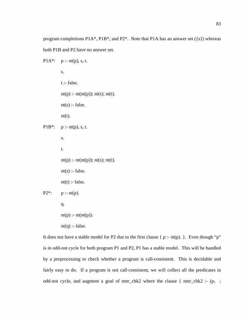
83

program completions P1A*, P1B*, and P2*. Note that P1A has an answer set ({s}) whereas

both P1B and P2 have no answer set.

P1A*: p :- nt(p), s, t.

s.

t :- false.

nt(p) :- nt(nt(p)); nt(s); nt(t).

nt(s) :- false.

nt(t).

P1B*: p :- nt(p), s, t.

s.

t.

nt(p) :- nt(nt(p)); nt(s); nt(t).

nt(s) :- false.

nt(t) :- false.

P2*: p :- nt(p).

q.

nt(p) :- nt(nt(p)).

nt(q) :- false.

It does not have a stable model for P2 due to the first clause { p :- nt(p). }. Even though “p”

is in odd-not cycle for both program P1 and P2, P1 has a stable model. This will be handled

by a preprocessing to check whether a program is call-consistent. This is decidable and

fairly easy to do. If a program is not call-consistent, we will collect all the predicates in

odd-not cycle, and augment a goal of nmr_chk2 where the clause { nmr_chk2 :- (p1 ;

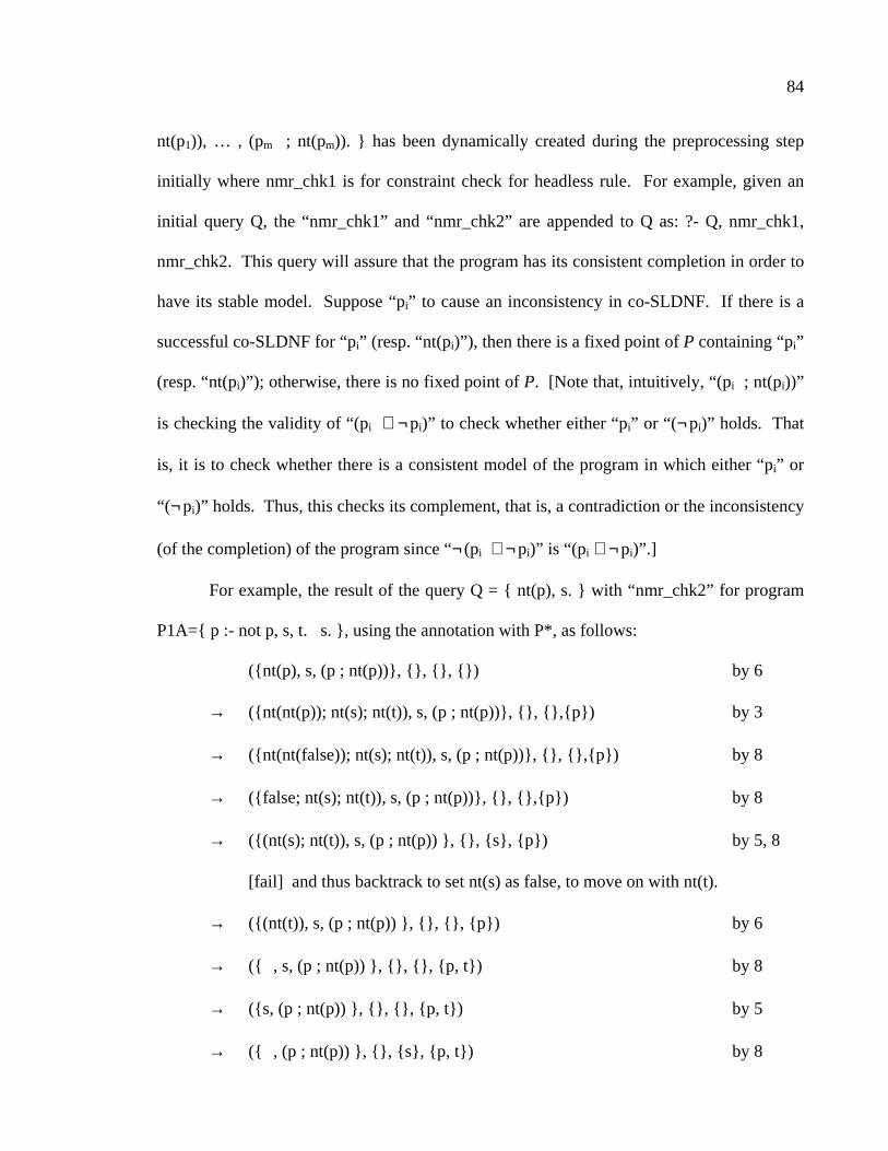
84

nt(p1)), … , (pm ; nt(pm)). } has been dynamically created during the preprocessing step

initially where nmr_chk1 is for constraint check for headless rule. For example, given an

initial query Q, the “nmr_chk1” and “nmr_chk2” are appended to Q as: ?- Q, nmr_chk1,

nmr_chk2. This query will assure that the program has its consistent completion in order to

have its stable model. Suppose “pi” to cause an inconsistency in co-SLDNF. If there is a

successful co-SLDNF for “pi” (resp. “nt(pi)”), then there is a fixed point of P containing “pi”

(resp. “nt(pi)”); otherwise, there is no fixed point of P. [Note that, intuitively, “(pi ; nt(pi))”

is checking the validity of “(pi ∨ ¬pi)” to check whether either “pi” or “(¬pi)” holds. That

is, it is to check whether there is a consistent model of the program in which either “pi” or

“(¬pi)” holds. Thus, this checks its complement, that is, a contradiction or the inconsistency

(of the completion) of the program since “¬(pi ∨ ¬pi)” is “(p i ∧ ¬pi)”.]

For example, the result of the query Q = { nt(p), s. } with “nmr_chk2” for program

P1A={ p :- not p, s, t. s. }, using the annotation with P*, as follows:

({nt(p), s, (p ; nt(p))}, {}, {}, {}) by 6

→ ({nt(nt(p)); nt(s); nt(t)), s, (p ; nt(p))}, {}, {},{p}) by 3

→ ({nt(nt(false)); nt(s); nt(t)), s, (p ; nt(p))}, {}, {},{p}) by 8

→ ({false; nt(s); nt(t)), s, (p ; nt(p))}, {}, {},{p}) by 8

→ ({(nt(s); nt(t)), s, (p ; nt(p)) }, {}, {s}, {p}) by 5, 8

[fail] and thus backtrack to set nt(s) as false, to move on with nt(t).

→ ({(nt(t)), s, (p ; nt(p)) }, {}, {}, {p}) by 6

→ ({����, s, (p ; nt(p)) }, {}, {}, {p, t}) by 8

→ ({s, (p ; nt(p)) }, {}, {}, {p, t}) by 5

→ ({����, (p ; nt(p)) }, {}, {s}, {p, t}) by 8

85

→ ({(p ; nt(p)) }, {}, {s}, {p, t}) by 3

→ ({nt(p)}, {}, {s}, {p, t}) by 2

→ ({}, {}, {s}, {p, t}) by 8

→ [success]

Similarly, the query={ s. } will succeed for P1A, augmented with “nmr_chk2”. However,

the result of the query Q = { nt(p), s. } with “nmr_chk2” for program P1B={ p :- not p, s, t.

s. t. } as follows:

{nt(p), s, (p ; nt(p))}, {}, {}, {}) by 6

→ ({nt(nt(p)); nt(s); nt(t)), s, (p ; nt(p))}, {}, {},{p}) by 3

→ ({nt(nt(false)); nt(s); nt(t)), s, (p ; nt(p))}, {}, {},{p}) by 8

→ ({false; nt(s); nt(t)), s, (p ; nt(p))}, {}, {},{p}) by 8

→ ({(nt(s); nt(t)), s, (p ; nt(p)) }, {}, {s}, {p}) by 6

→ [fail] and thus backtrack to set nt(s) as false, to move on with nt(t).

→ ({nt(t), s, (p ; nt(p)) }, {}, {}, {p}) by 6

→ [fail]

Similarly for P2 = { p :- nt(p). q. }, the query { q.} with “nmr_chk2” will have a failed

derivation.

({q, (p ; nt(p))}, {}, {}, {}) by 5

→ ({(p ; nt(p))}, {}, {q},{}) by 5

→ ({(nt(p) ; nt(p))}, {}, {p, q},{}) by 4

→ ({nt(����) ; nt(p))}, {}, {p, q},{}) by 8

→ ({nt(p))}, {}, {p, q},{}) by 4

86

→ ({nt(����)}, {}, {p, q},{}) by 8

→ [fail]

Further, as noted earlier for P1, there are a few partial models of {s}, {t}, {s, t}, even though

there is no stable model due to the inconsistency caused by p with the clause { p :- not p, s,

t. }. Thus the following query will detect any partial model for the query Q, if exists.

?- Q, nmr_chk1.

Finally, as we noted previously, the difference between the rational Herbrand model of co-

LP and the minimal Herbrand model (lfp) of ASP can be resolved via loop formulas (Lin

and Zhao 2002) as the loop formulas can be easily computed with a co-SLDNF trace at the

end of each successful co-SLDNF derivation given the initial query. Thus the task of

solving ASP programs top-down and goal-directed is four-fold as we noted earlier: (1) to

find a partial model with co-SLDNF, (2) to eliminate loop-positive solution, to be minimal,

(3) to handle constraint rules and its integrity check, and (4) to check for a total model, with

a preprocessing and a post-processing.

4.4 Coinductive ASP Solver

To summarize, the co-ASP solver’s strategy is first to transform an ASP program into a

coinductive ASP (co-ASP) program and use the following solution-strategy:

(1) Compute the completion of the program and then execute the query goal using co-

SLDNF resolution on the completed program (this may yield a partial model).

(2) Avoid loop-positive solution (for example, p derived coinductively from rules such as {

p :- p. }) during co-SLDNF resolution: This is achieved during execution by ensuring

that coinductive success is allowed while exercising the coinductive hypothesis rule only

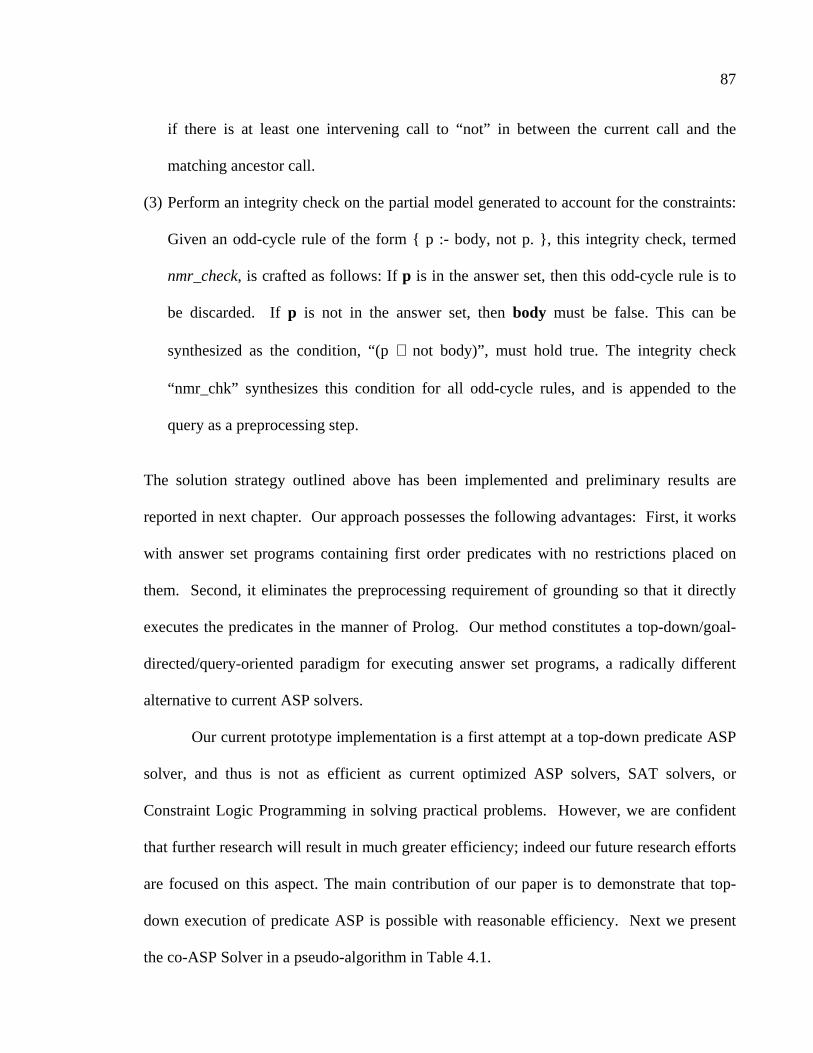
87

if there is at least one intervening call to “not” in between the current call and the

matching ancestor call.

(3) Perform an integrity check on the partial model generated to account for the constraints:

Given an odd-cycle rule of the form { p :- body, not p. }, this integrity check, termed

nmr_check, is crafted as follows: If p is in the answer set, then this odd-cycle rule is to

be discarded. If p is not in the answer set, then body must be false. This can be

synthesized as the condition, “(p ∨ not body)”, must hold true. The integrity check

“nmr_chk” synthesizes this condition for all odd-cycle rules, and is appended to the

query as a preprocessing step.

The solution strategy outlined above has been implemented and preliminary results are

reported in next chapter. Our approach possesses the following advantages: First, it works

with answer set programs containing first order predicates with no restrictions placed on

them. Second, it eliminates the preprocessing requirement of grounding so that it directly

executes the predicates in the manner of Prolog. Our method constitutes a top-down/goal-

directed/query-oriented paradigm for executing answer set programs, a radically different

alternative to current ASP solvers.

Our current prototype implementation is a first attempt at a top-down predicate ASP

solver, and thus is not as efficient as current optimized ASP solvers, SAT solvers, or

Constraint Logic Programming in solving practical problems. However, we are confident

that further research will result in much greater efficiency; indeed our future research efforts

are focused on this aspect. The main contribution of our paper is to demonstrate that top-

down execution of predicate ASP is possible with reasonable efficiency. Next we present

the co-ASP Solver in a pseudo-algorithm in Table 4.1.

88

Table 4.1. Co-ASP Solver (in pseudo-code).

Co-ASP Solver(Input: ASP Program P, query Q; Output: Answer Set AS).

%% Preprocessing Given input program P, Build predicate dependency graph PDP of P. % Note: the algorithm to build a dependency graph and find a path between two % nodes are well-known and standard; thus it is which is skipped here. Find all predicates in odd-not cycle in PDF into a set: OddNot. If OddNot is empty Then set “nmr_chk2.” Set P* to be P. Else Set nmr_chk2_body = empty-string. For each predicate of arity n, p/n, in OddNot Append (p(Xn) ; nt(p(Xn)) to nmr_chk2_body where p(Xn) is predicate p with Xn is n-terms of distinct variables. End-For Set “nmr_chk2 :- nmr_chk2_body.” If (nmr_chk2) Then message “P has a Herbrand model” Else message “P does not have a Herbrand model” End-if Generate negated definition of P, to be augmented with P to be P*. End-if Find all headless rules (G1 or … or Gm) into a set: Headless If Headless is empty, Then set “nmr_chk1.” Else Set nmr_chk1_body = empty-string For each Gi in Headless Set falsei :- Gi. Append nt(falsei ) to nmr_chk1_body. End-for Set “nmr_chk1 :- nmr_chk1_body.” End-if % End of Preprocessing Given input query Q, augment Q with nmr_chk1 and nmr_chk2 to be Q* Given query Q* and program P*, Run co-SLDNF on Query and keeping its path-trace. For each subgoal of Query successful,

89

Table 4.1 continued

If current path-trace is loop-positive Then it is not minimal thus false to be backtracked Else it is minimal and to continue End-For If successful co-SLDNF derivation with X+ and X-, resulting in AS with backtracking Then message “An Answer Set found” output AS. Else message “No (more) Answer Set” End-If % end of ASP Solver

4.5 Correctness of Co-ASP Solver

In this section, the soundness and completeness results for co-ASP Solver are presented.

Theorem 4.1 Completeness of co-ASP Solver for a program with a stable model: If P is a

general ASP program with a stable model M in the rational Herbrand base of P, then a query

Q consistent with M has a successful co-ASP solution (of an answer set). �

Proof. Let P be a general ASP program with a stable model M in the rational Herbrand

base of P. Then by Theorem 3.1 (3), (4), and (7) (Fages 1994: Propositions 4.4 and 4.5,

Corollary 3.6), M is a fixed point and a Herbrand model of comp(P) which also implies that

P has a consistent comp(P). That is, the query Q consistent with M will have a successful

co-SLDNF derivation (D). Further if D, with the atoms p and q, has a positive loop (that is,

a non-empty path from an atom p to q with all edges positive), then by a trace check of the

derivation path, by checking for call-consistent and free of positive loop (that is, loop

formulas of Lin and Zhao (2002)), co-ASP Solver will reject this co-SLDNF derivation

90

whose resulting answer is not minimal (that is, not a stable model). Therefore by

completeness of Theorem 3.4, the query Q consistent with M has a successful co-ASP

solution which has a successful co-SLDNF derivation of a partial model, consistent with M,

that is, a stable model). �

Theorem 4.2 (Soundness of co-ASP Solver for a program which is call-consistent or order-

consistent): Let P be a general ASP program which is call-consistent or order-consistent. If

a query Q has a successful co-ASP solution, then Q is a subset of an answer set. �

Proof. The proof is straightforward from Theorem 3.1 (5)-(7) (Fages 1994: Corollary 3.6,

Theorem 4.6 and 5.4) and that a successful co-ASP solution is free of loop-positive (loop

formulas). �

Note that the assumptions of the completeness and soundness theorems do not

require the nonmonotonic checking of inconsistency (that is, “nmr_chk2” of co-ASP

Solver). Further for the class of propositional (or grounded) ASP programs, it is decidable

to check for each predicate p of a program P for its call-consistency in the predicate

dependency graph of P. The nonmonotonic check (“nmr_chk2” of co-ASP Solver of p’s,

that is, (p or not p)) will assure the program P whether P has a stable model or not. This

check can be done once for all, as a preprocessing. For predicate ASP programs, if a

program P is call-consistent or order-consistent, then Theorem 4.2 assures the soundness.

However, there is still a large class of predicate ASP programs which are not under this

restriction, waiting to be investigated.

We note that the limitation of our current approach in inconsistency-checking is

restricted to the class of predicate ASP programs of call-consistent or order-consistent. Our

91

future works for co-LP include (1) a language specification of co-LP with coinductive built-

in predicates and system libraries, (2) its optimization and tuning, and (3) its extension to

concurrent and parallel processing. Our future works for co-ASP Solver include (1) a fully

automated and optimized co-ASP Solver, (2) a utility to transform a ASP program into a co-

ASP program, (3) a utility to check inconsistency of ASP program extending current

restriction, and (4) extending a range of ASP applications with performance monitoring and

benchmarking.

92

CHAPTER 5

APPLICATIONS OF CO-ASP SOLVER

5.1 Introduction

In this chapter, we present some examples of ASP programs which have been implemented

and solved successfully by co-ASP Solver. These examples are found in the ASP literature

(Baral 2003; Niemelä and Simons. 1996a; Dovier, Formisano, and Pontelli 2005), Internet

sites1, or available to the authors through our personal correspondences. Interestingly, most

of these examples are call-consistent and free of odd-not cycle. As a result, “nmr_chk2” (for

odd-not cycle) is essentially a trivial fact (without a body). All of these examples are

successfully implemented as shown here, tested and verified for ASP Solver. Most of the

ASP examples can run directly under co-ASP Solver almost without any modification or

transformation. For example, all the programs in chapter 3 are the ASP programs that can

run with very minor modification. As noted in chapter 4, there are two cases of ASP

programs which require the additional preprocessing for (1) headless constraint rules and (2)

constraint rules in odd-not cycle, for the relevancy requirement of LP. There are two

implementations of ASP Solver: (1) one fully automated to transform a ground ASP program

(where grounding is done by Lparse) and (2) the other with a predicate ASP (with a few

minor preprocessing steps as noted in the previous section). Note that “nnot(_)” is the body

of a clause is “nt(_)”, and by this we distinguish “nnot(_)” in the body of a clause and “nt(_)”

1 For example, http://www.tcs.hut.fi/Software/index.shtml#benchmarks

93

as the corresponding head-atom of negated definition of it for current implementation (a

meta-interpreter) of ASP Solver, and to distinguish it from “not” (or “\+”, the negation

operator in Prolog). We illustrate our top-down system via some example programs and

queries. Most of the small ASP examples2 and their queries run very fast, usually under

0.0001 CPU seconds. Our test environment is implemented on top of YAP Prolog3 running

under Linux in a shared environment with dual core AMD Opteron Processor 275, with

2GHz with 8GB memory. We elaborate some of the examples for the performance in the

next chapter.

5.2 Simple and Classical ASP Examples

The first three examples are relatively small and to be grounded (via Lparse), to be

transformed into co-ASP programs. The transforming program is implemented in Perl to

read a grounded ASP program to produce co-ASP program to be processed by co-ASP

Solver. The performance of co-ASP Solver is close to ASP Solvers.

Example 5.1 Our first example is “move-win,” a program that computes the winning path

in a simple game, tested successfully with various test queries, as listed in Table 5.1. This is

also an example of the predicate ASP programs which do not require any preprocessing but

can be run directly under co-ASP Solver. For the benefit of the comparison, we list the

propositional co-ASP program of “move-win” in Table 5.2.

2 More examples and performance data can be found from our Technical Report available: http://www.utdallas.edu/~rkm010300/research/co-ASP.pdf

3 http://www.dcc.fc.up.pt/~vsc/Yap/

94

Table 5.1. move-win program

% The original predicate ASP “move-win” program move(a,b). move(b,a). move(a,c). move(c,d). move(d,e). move(c,f). move(e,f). win(X) :- move(X,Y), not win(Y).

The “move-win” program consists of two parts: (a) facts of “move(x,y)” (to allow a move

from x to y), and (b) a rule { win(X) :- move(X,Y), not win(Y). }. The second part infers X

to be a winner if there is a move from X to Y, and Y is not a winner. This is a predicate ASP

program which is not call-consistent but order-consistent. It has two answer sets: (a) {

win(a), win(c), win(e), move(e,f), move(d,e), move(c,f), move(c,d), move(b,a), move(a,c),

move(a,b) } and (b) { win(b), win(c), win(e), move(e,f), move(d,e), move(c,f), move(c,d),

move(b,a), move(a,c), move(a,b) }.

Figure 5.1. Predicate-Dependency Graph of Predicate ASP “move-win”.

The program has an odd-not cycle with respect to the predicate “win/1”. After grounding,

the ground program is free of odd-not cycle. After the grounding, “move-win” co-ASP

program is generated as follows:

not

win(X) move(X,Y)

95

Table 5.2. move-win program - ground

%% Transformed propositional co-ASP “move-win”. :- coinductive(win/1). move(a,b). move(a,c). move(b,a). move(c,d). move(c,f). move(d,e). move(e,f). win(a) :- nnot(win(b)), move(a,b). win(a) :- nnot(win(c)), move(a,c). win(b) :- nnot(win(a)), move(b,a). win(c) :- nnot(win(d)), move(c,d). win(c) :- nnot(win(f)), move(c,f). win(d) :- nnot(win(e)), move(d,e). win(e) :- nnot(win(f)), move(e,f). %% the following is the negated definitions. nt(win(a)) :- ( win(c) ; nnot(move(a,c)) ), ( win(b) ; nnot(move(a,b)) ). nt(win(b)) :- ( win(a) ; nnot(move(b,a)) ). nt(win(c)) :- ( win(f) ; nnot(move(c,f)) ), ( win(d) ; nnot(move(c,d)) ). nt(win(d)) :- ( win(e) ; nnot(move(d,e)) ). nt(win(e)) :- ( win(f) ; nnot(move(e,f)) ). nmr_chk :- nmr_chk1, nmr_chk2. nmr_chk1. nmr_chk2. init:- move(a,b), move(a,c), move(b,a), move(c,d), move(c,f), move(d,e), move(e,f).

There is no body for the headless constraint rule. This makes nmr_chk1 and nmr_chk2 to be

a trivial fact. Further, “init” clause will load all the facts into the positive table, to make the

inference purely coinductive.

96

Figure 5.2. Atom-Dependency Graph of Propositional “move-win”.

Figure 5.2 shows that there is no odd-not cycle in this program which is order-consistent with

respect to {win(c), win(d), win(f), win(e)} and call-consistent with respect to {win(a),

win(b)}. There is no integrity check required. Further since there is no headless rule, the

original ASP predicate program of move-win can run under co-ASP solver with minimum

modification. Further note that “init” clause will load all the facts into the positive table, to

make the inference purely coinductive.

Some of the sample queries for the ground ASP program of this move-win program

are listed in Table 5.3. The clauses of q1a – q9a and q1b – q9b are the test queries where q1a

– q3a and q1b – q3b are the only successful queries. As noted earlier, two stable model

should contain { win(a), win(c), win(e) } or { win(b), win(c), win(e) }, respectively.

Therefore any partial model (partial answer set) will have a successful derivation.

not

not

not

win(a) win(b)

not

win(c)

win(f)

win(d)

not

win(e)

not

not

97

Table 5.3. move-win program – query examples

q1a :- win(a), nmr_chk. q2a :- win(a), win(c), nmr_chk. q3a :- win(a), win(c), win(e), nmr_chk. q4a :- win(a), win(f), nmr_chk. q5a :- win(f), nmr_chk. q6a :- win(a), win(c), win(f), nmr_chk. q7a :- win(d), nmr_chk. q8a :- win(a), win(d), nmr_chk. q9a :- win(a), win(c), win(d), nmr_chk. q1b :- win(b), nmr_chk. q2b :- win(b), win(c), nmr_chk. q3b :- win(b), win(c), win(e), nmr_chk. q4b :- win(b), win(f), nmr_chk. q5b :- win(f), nmr_chk. q6b :- win(b), win(c), win(f), nmr_chk. q7b :- win(b), win(d), nmr_chk. q8b :- win(b), win(d), nmr_chk. q9b :- win(b), win(c), win(d), nmr_chk.

There are two clauses for “win(a)” as head-atom.

win(a) :- nnot(win(b)), move(a,b).

win(a) :- nnot(win(c)), move(a,c).

Its positive definition of “win(a)” in one clause is then:

win(a) :- (nnot(win(b)), move(a,b));

(nnot(win(c)), move(a,c)).

The negated definition of “win(a)” is then:

nt(win(a)) :- nt((nnot(win(b)), move(a,b));

(nnot(win(c)), move(a,c))).

This clause for “nt(win(a))” is simplified further as:

nt(win(a)):- ( win(c) ; nnot(move(a,c)) ),

( win(b) ; nnot(move(a,b)) ).

98

Let us consider the query “q1a” = ?- init, win(a) will generate the following successful co-

SLDNF derivation. The “init” clause will load the coinductive positive table, χ+ =

{ move(a,b),move(a,c),move(b,a),move(c,d),move(c,f),m ove(d,e),m

ove(e,f) }. (Note that we show the co-SLDNF derivations on the lefthand side with “→”

and the annotation using co-SLDNF resolution step on the righthand side (and the following

lines if more annotation or comment is needed.)

→ ({ win(a) }, {}, χ+, {}). by (5) with win(a).

→ ({ ( nnot(win(b)), move(a,b) ); ( nnot(win(c)), move(a,c) ) }, {}, {win(a)} ∪ χ+, {}).

by (5) with nnot(win(b))

→ ({ ( (win(a); nnot(move(b,a)), move(a,b) ); (nnot(win(c)), move(a,c)) },

{}, {win(a)} ∪ χ+, {win(b)}). by (1) coinductive success for win(a)

→ ({ move(a,b); (nnot(win(c)), move(a,c)) }, {}, {move(a,b), win(a)} ∪ χ+, {win(b)}).

by (1) coinductive success for move(a,b)

→ [success]

Next consider the query “q7a” = ?- win(d) will generate the following failed co-SLDNF

derivation.

→ ({ win(d) }, {}, {}, {}). by (5) with win(d).

→ ({ ( nnot(win(e)), move(d,e) ) }, {}, {win(d)}, {}). by (5) with nnot(win(e))

→ ({ ( (win(f); nnot(move(e,f))), move(d,e) ) }, {}, {win(a), win(d)} ∪ χ+, {win(e)}).

by (7) no rule for win(f)

→ ({ nnot(move(e,f)), move(d,e) }, {}, {win(a), win(d)} ∪ χ+, {win(e)}).

by (4) coinductive failure for win(e,f) in χ+.

→ [fail]

99

We have the correct results with the test queries with the predicate “move-win” co-ASP

program.

Table 5.4. move-win as a predicate co-ASP program

% The original predicate ASP “move-win” program move(a,b). move(b,a). move(a,c). move(c,d). move(d, e). move(c,f). move(e,f). win(X) :- move(X,Y), not win(Y).

For example, the derivation for query ?- win(a) is then:

→ ({ win(a) }, {}, χ+, {}). by (5) and the clause: win(a).

win(X) :- move(X,Y), not win(Y).

t1: X’=a

win(a) :- move(a,Y), not win(Y).

→ ({ move(a,Y), not win(Y) }, {t1}, {win(a)}, {}).

by (5) and the clause: move(a,Y) to be unified with move(a,b)

move(a,b).

t2: Y’=b

→ ({ not win(b) }, {t1, t2}, {move(a,b), win(a)}, {}).

by (6) and the clause: win(X) :- move(X,Y), not win(Y).

not( win(X)) => not( move(X,Y), not win(Y). )

t3: X’’=b

not( win(b)) => not( move(b,Y), not win(Y). )

→ ({ not ( move(b,Y), not win(Y) ) }, {t1, t2, t3}, {move(a,b), win(a)}, {}).

by (6) and the clause: move(b,Y)

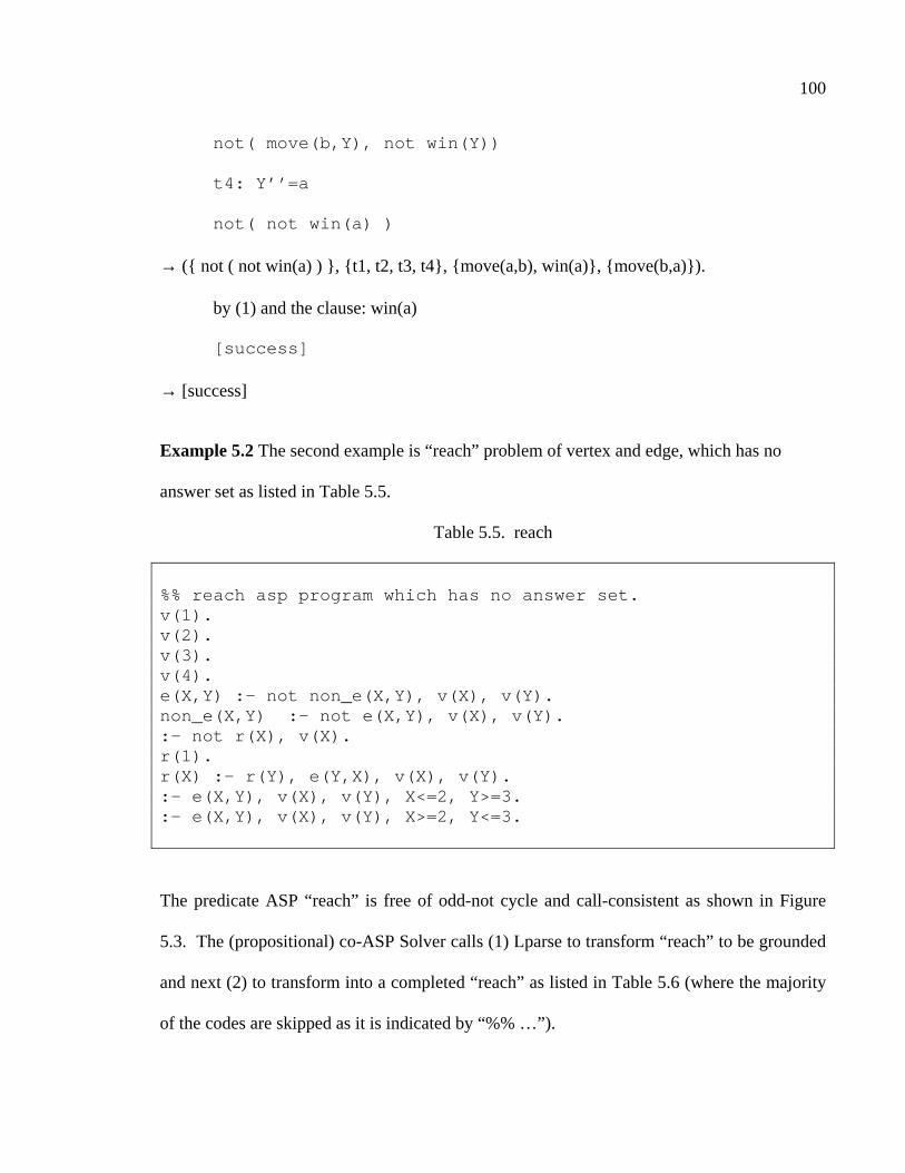
100

not( move(b,Y), not win(Y))

t4: Y’’=a

not( not win(a) )

→ ({ not ( not win(a) ) }, {t1, t2, t3, t4}, {move(a,b), win(a)}, {move(b,a)}).

by (1) and the clause: win(a)

[success]

→ [success]

Example 5.2 The second example is “reach” problem of vertex and edge, which has no

answer set as listed in Table 5.5.

Table 5.5. reach

%% reach asp program which has no answer set. v(1). v(2). v(3). v(4). e(X,Y) :- not non_e(X,Y), v(X), v(Y). non_e(X,Y) :- not e(X,Y), v(X), v(Y). :- not r(X), v(X). r(1). r(X) :- r(Y), e(Y,X), v(X), v(Y). :- e(X,Y), v(X), v(Y), X<=2, Y>=3. :- e(X,Y), v(X), v(Y), X>=2, Y<=3.

The predicate ASP “reach” is free of odd-not cycle and call-consistent as shown in Figure

5.3. The (propositional) co-ASP Solver calls (1) Lparse to transform “reach” to be grounded

and next (2) to transform into a completed “reach” as listed in Table 5.6 (where the majority

of the codes are skipped as it is indicated by “%% …”).

101

Figure 5.3. Predicate-dependency graph of Predicate ASP “reach”

Table 5.6. reach - propositional co-ASP program

:- coinductive(e/2). %% false -- for headless constraint rules :- coinductive(non_e/2). :- coinductive(r/1). :- coinductive(v/1). r(1). v(1). v(2). v(3). v(4). anset :- nnot(r(1)), nnot(r(2)), nnot(r(3)), nnot( r(4)). e(1,1) :- nnot(non_e(1,1)), v(1), v(1). e(1,2) :- nnot(non_e(1,2)), v(1), v(2). e(1,3) :- nnot(non_e(1,3)), v(1), v(3). e(1,4) :- nnot(non_e(1,4)), v(1), v(4). %% ... %% the rest of the code is skipped here. non_e(1,1) :- nnot(e(1,1)), v(1), v(1). non_e(1,2) :- nnot(e(1,2)), v(1), v(2). non_e(1,3) :- nnot(e(1,3)), v(1), v(3). non_e(1,4) :- nnot(e(1,4)), v(1), v(4). %% ... %% the rest of the code is skipped here. r(1) :- r(1), e(1,1), v(1), v(1). r(1) :- r(2), e(2,1), v(1), v(2). r(1) :- r(3), e(3,1), v(1), v(3). r(1) :- r(4), e(4,1), v(1), v(4). %% ... %% the rest of the code is skipped here. nt(e(1,1)) :- ( non_e(1,1) ; nnot(v(1)) ; nnot(v (1)) ). nt(e(1,2)) :- ( non_e(1,2) ; nnot(v(1)) ; nnot(v (2)) ). nt(e(1,3)) :- ( non_e(1,3) ; nnot(v(1)) ; nnot(v (3)) ). nt(e(1,4)) :- ( non_e(1,4) ; nnot(v(1)) ; nnot(v (4)) ). %% ... %% the rest of the code is skipped here. nt(non_e(1,1)) :- ( e(1,1) ; nnot(v(1)) ; nnot(v (1)) ). nt(non_e(1,2)) :- ( e(1,2) ; nnot(v(1)) ; nnot(v (2)) ).

not

e(X) not_e(X,Y)

not

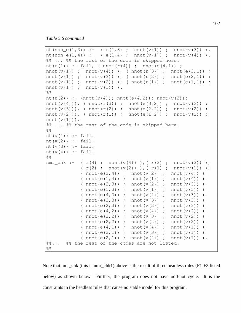
102

Table 5.6 continued

nt(non_e(1,3)) :- ( e(1,3) ; nnot(v(1)) ; nnot(v (3)) ). nt(non_e(1,4)) :- ( e(1,4) ; nnot(v(1)) ; nnot(v (4)) ). %% ... %% the rest of the code is skipped here. nt(r(1)) :- fail, ( nnot(r(4)) ; nnot(e(4,1)) ; nnot(v(1)) ; nnot(v(4)) ), ( nnot(r(3)) ; nnot(e( 3,1)) ; nnot(v(1)) ; nnot(v(3)) ), ( nnot(r(2)) ; nnot(e( 2,1)) ; nnot(v(1)) ; nnot(v(2)) ), ( nnot(r(1)) ; nnot(e( 1,1)) ; nnot(v(1)) ; nnot(v(1)) ). %% nt(r(2)) :- (nnot(r(4)); nnot(e(4,2)); nnot(v(2)); nnot(v(4))), ( nnot(r(3)) ; nnot(e(3,2)) ; nnot(v (2)) ; nnot(v(3))), ( nnot(r(2)) ; nnot(e(2,2)) ; nnot(v (2)) ; nnot(v(2))), ( nnot(r(1)) ; nnot(e(1,2)) ; nnot(v (2)) ; nnot(v(1))). %% ... %% the rest of the code is skipped here. %% nt(v(1)) :- fail. nt(v(2)) :- fail. nt(v(3)) :- fail. nt(v(4)) :- fail. %% nmr_chk :- ( r(4) ; nnot(v(4)) ),( r(3) ; nnot(v (3)) ), ( r(2) ; nnot(v(2)) ),( r(1) ; nnot(v (1)) ), ( nnot(e(2,4)) ; nnot(v(2)) ; nnot(v( 4)) ), ( nnot(e(1,4)) ; nnot(v(1)) ; nnot(v( 4)) ), ( nnot(e(2,3)) ; nnot(v(2)) ; nnot(v( 3)) ), ( nnot(e(1,3)) ; nnot(v(1)) ; nnot(v( 3)) ), ( nnot(e(4,3)) ; nnot(v(4)) ; nnot(v( 3)) ), ( nnot(e(3,3)) ; nnot(v(3)) ; nnot(v( 3)) ), ( nnot(e(2,3)) ; nnot(v(2)) ; nnot(v( 3)) ), ( nnot(e(4,2)) ; nnot(v(4)) ; nnot(v( 2)) ), ( nnot(e(3,2)) ; nnot(v(3)) ; nnot(v( 2)) ), ( nnot(e(2,2)) ; nnot(v(2)) ; nnot(v( 2)) ), ( nnot(e(4,1)) ; nnot(v(4)) ; nnot(v( 1)) ), ( nnot(e(3,1)) ; nnot(v(3)) ; nnot(v( 1)) ), ( nnot(e(2,1)) ; nnot(v(2)) ; nnot(v( 1)) ). %%... %% the rest of the codes are not listed. %%

Note that nmr_chk (this is nmr_chk1) above is the result of three headless rules (F1-F3 listed

below) as shown below. Further, the program does not have odd-not cycle. It is the

constraints in the headless rules that cause no stable model for this program.

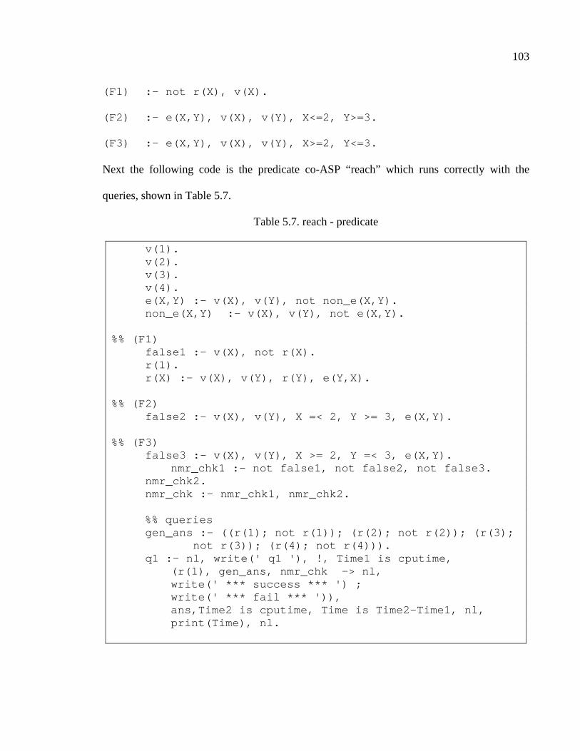
103

(F1) :- not r(X), v(X).

(F2) :- e(X,Y), v(X), v(Y), X<=2, Y>=3.

(F3) :- e(X,Y), v(X), v(Y), X>=2, Y<=3.

Next the following code is the predicate co-ASP “reach” which runs correctly with the

queries, shown in Table 5.7.

Table 5.7. reach - predicate

v(1). v(2). v(3). v(4). e(X,Y) :- v(X), v(Y), not non_e(X,Y). non_e(X,Y) :- v(X), v(Y), not e(X,Y). %% (F1) false1 :- v(X), not r(X). r(1). r(X) :- v(X), v(Y), r(Y), e(Y,X). %% (F2) false2 :- v(X), v(Y), X =< 2, Y >= 3, e(X,Y). %% (F3) false3 :- v(X), v(Y), X >= 2, Y =< 3, e(X,Y).

nmr_chk1 :- not false1, not false2, not false3. nmr_chk2.

nmr_chk :- nmr_chk1, nmr_chk2. %% queries

gen_ans :- ((r(1); not r(1)); (r(2); not r(2)); (r (3); not r(3)); (r(4); not r(4))). q1 :- nl, write(' q1 '), !, Time1 is cputime,

(r(1), gen_ans, nmr_chk -> nl, write(' *** success *** ') ;

write(' *** fail *** ')), ans,Time2 is cputime, Time is Time2-Time1, nl, print(Time), nl.

104

Example 5.3 The third example is a typical case to show the loop formulas and the

difference between lfp and gfp semantics, dealing with positive and negative loops.

Table 5.8. ASP program abc for lfp and gfp

a :- b. b :- a. a :- not c. c :- d. d :- c. c :- not a.

Figure 5.4. Predicate-dependency graph of Predicate ASP abc.

The dependency graph shows that the pairs of { a, b } and { c, d } are in a positive loop

(loop-positive) whereas the pair of (a, c) is in a negative loop (even-not cycle and call-

consistent). This loop-positive condition prevents the pairs ({a, b} or {c, d}) to be contained

in a stable model. Therefore there is no stable model containing either a pair of { a, b } or {

c, d }. However, the pair { a, c } is in even-not cycle (call-consistent). For this reason, the

pair {a, c} is the only stable model for this program. If a Herbrand model which is not

minimal is considered, then {a, b} and {c, d} can be in a Herbrand model (with maximal

fixed point semantics). In this case, we have several Herbrand models including {a, b}, {c,

d}, {a, c} and {a, b, c, d}.

not

b a

not

c d

105

Table 5.9. co-ASP program for abc

:- coinductive(a/0). :- coinductive(b/0). :- coinductive(c/0). :- coinductive(d/0). a :- b. b :- a. a :- nnot(c). c :- d. d :- c. c :- nnot(a). %% The negative definition is provided but not requ ired. nt(a):- c, nnot(b). nt(b):- nnot(a). nt(c):- a, nnot(d). nt(d):- nnot(c).

The following co-SLDNF “trace” history and check shows the result of query ?- a. according

to stable model semantics (by preventing any loop-positive assertion).

?- a.

** check_trace TQ=[ a,b,a] for S=a

Here the first derivation is taking the clause { a :- b. b :- a. }, thus to be failed after detecting

that there is no negation in the path from the goal to current successful end-node (that is, the

path from “a” via “b” to “a”). Then it will fail and backtrack to try the next possibility using

{ a :- not c. c :- not a. }, thus to be successful, as there is a negated atom in the path (of [a,

not c, a]) as shown below.

** check_trace TQ=[ a,nnot(c),a] for S=a

** Succ Trace S2R: [nnot(c)]

yes

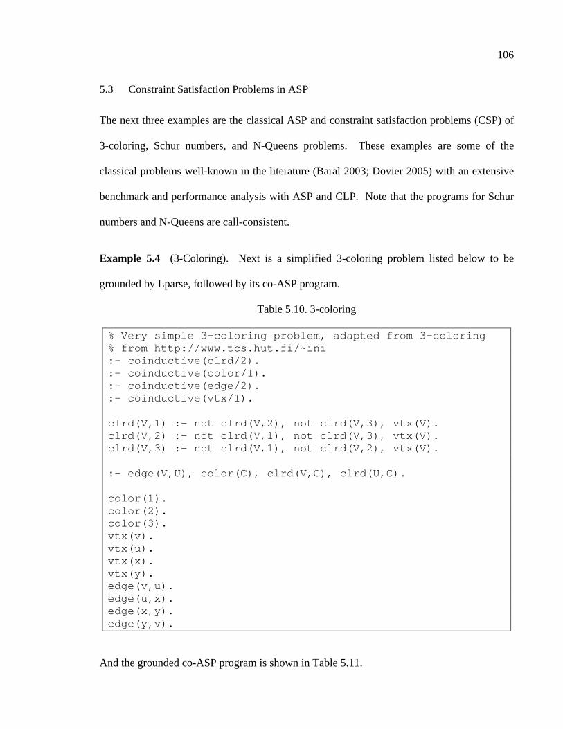
106

5.3 Constraint Satisfaction Problems in ASP

The next three examples are the classical ASP and constraint satisfaction problems (CSP) of

3-coloring, Schur numbers, and N-Queens problems. These examples are some of the

classical problems well-known in the literature (Baral 2003; Dovier 2005) with an extensive

benchmark and performance analysis with ASP and CLP. Note that the programs for Schur

numbers and N-Queens are call-consistent.

Example 5.4 (3-Coloring). Next is a simplified 3-coloring problem listed below to be

grounded by Lparse, followed by its co-ASP program.

Table 5.10. 3-coloring

% Very simple 3-coloring problem, adapted from 3-co loring % from http://www.tcs.hut.fi/~ini :- coinductive(clrd/2). :- coinductive(color/1). :- coinductive(edge/2). :- coinductive(vtx/1). clrd(V,1) :- not clrd(V,2), not clrd(V,3), vtx(V). clrd(V,2) :- not clrd(V,1), not clrd(V,3), vtx(V). clrd(V,3) :- not clrd(V,1), not clrd(V,2), vtx(V). :- edge(V,U), color(C), clrd(V,C), clrd(U,C). color(1). color(2). color(3). vtx(v). vtx(u). vtx(x). vtx(y). edge(v,u). edge(u,x). edge(x,y). edge(y,v).

And the grounded co-ASP program is shown in Table 5.11.

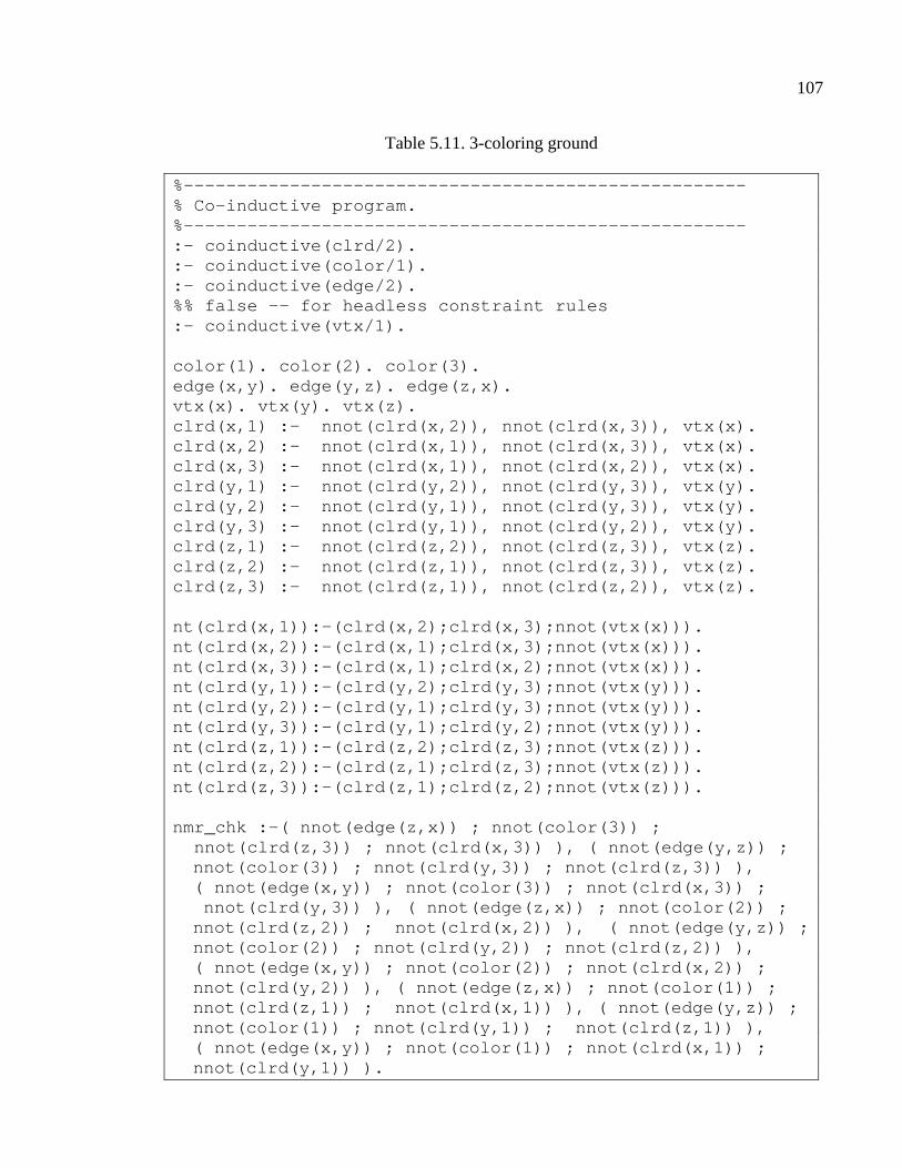
107

Table 5.11. 3-coloring ground

%-------------------------------------------------- --- % Co-inductive program. %-------------------------------------------------- --- :- coinductive(clrd/2). :- coinductive(color/1). :- coinductive(edge/2). %% false -- for headless constraint rules :- coinductive(vtx/1). color(1). color(2). color(3). edge(x,y). edge(y,z). edge(z,x). vtx(x). vtx(y). vtx(z). clrd(x,1) :- nnot(clrd(x,2)), nnot(clrd(x,3)), vtx (x). clrd(x,2) :- nnot(clrd(x,1)), nnot(clrd(x,3)), vtx (x). clrd(x,3) :- nnot(clrd(x,1)), nnot(clrd(x,2)), vtx (x). clrd(y,1) :- nnot(clrd(y,2)), nnot(clrd(y,3)), vtx (y). clrd(y,2) :- nnot(clrd(y,1)), nnot(clrd(y,3)), vtx (y). clrd(y,3) :- nnot(clrd(y,1)), nnot(clrd(y,2)), vtx (y). clrd(z,1) :- nnot(clrd(z,2)), nnot(clrd(z,3)), vtx (z). clrd(z,2) :- nnot(clrd(z,1)), nnot(clrd(z,3)), vtx (z). clrd(z,3) :- nnot(clrd(z,1)), nnot(clrd(z,2)), vtx (z). nt(clrd(x,1)):-(clrd(x,2);clrd(x,3);nnot(vtx(x))). nt(clrd(x,2)):-(clrd(x,1);clrd(x,3);nnot(vtx(x))). nt(clrd(x,3)):-(clrd(x,1);clrd(x,2);nnot(vtx(x))). nt(clrd(y,1)):-(clrd(y,2);clrd(y,3);nnot(vtx(y))). nt(clrd(y,2)):-(clrd(y,1);clrd(y,3);nnot(vtx(y))). nt(clrd(y,3)):-(clrd(y,1);clrd(y,2);nnot(vtx(y))). nt(clrd(z,1)):-(clrd(z,2);clrd(z,3);nnot(vtx(z))). nt(clrd(z,2)):-(clrd(z,1);clrd(z,3);nnot(vtx(z))). nt(clrd(z,3)):-(clrd(z,1);clrd(z,2);nnot(vtx(z))). nmr_chk :-( nnot(edge(z,x)) ; nnot(color(3)) ; nnot(clrd(z,3)) ; nnot(clrd(x,3)) ), ( nnot(edge( y,z)) ;

nnot(color(3)) ; nnot(clrd(y,3)) ; nnot(clrd(z,3)) ), ( nnot(edge(x,y)) ; nnot(color(3)) ; nnot(clrd(x,3) ) ; nnot(clrd(y,3)) ), ( nnot(edge(z,x)) ; nnot(color( 2)) ; nnot(clrd(z,2)) ; nnot(clrd(x,2)) ), ( nnot(edge( y,z)) ; nnot(color(2)) ; nnot(clrd(y,2)) ; nnot(clrd(z,2)) ), ( nnot(edge(x,y)) ; nnot(color(2)) ; nnot(clrd(x,2) ) ; nnot(clrd(y,2)) ), ( nnot(edge(z,x)) ; nnot(color(1 )) ; nnot(clrd(z,1)) ; nnot(clrd(x,1)) ), ( nnot(edge(y ,z)) ; nnot(color(1)) ; nnot(clrd(y,1)) ; nnot(clrd(z,1)) ), ( nnot(edge(x,y)) ; nnot(color(1)) ; nnot(clrd(x,1) ) ; nnot(clrd(y,1)) ).

108

Example 5.5 (Schur Number). Next is Schur NxB (for N numbers with B boxes). The

problem is to find a combination of N numbers (consecutive integers from 1 to N) for B

boxes (consecutive integers from 1 to B) with one rule and two constraints. The first rule is

that a number X should be paired with one and only one box Y. The first constraint is that if

a number X is paired with a box B, then its double-number, X+X, should not be paired with

the box B. The second constraint is that if two numbers, X and Y, are paired with a box B,

then its sum-number, X+Y, should not be paired with the box B.

Table 5.12. Schur NxB

%% The original ASP Schur NxB Program. box(1). box(2). box(3). box(4). box(5). num(1). num(2). num(3). num(4). num(5). num(6). num(7). num(8). num(9). num(10). num(11). num(12). in(X,B) :- num(X), box(B), not not_in(X,B). not_in(X,B) :- num(X),box(B),box(BB),B ≠ BB,in(X,BB). :- num(X), box(B), in(X,B), in(X+X,B). :- num(X), num(Y), box(B), in(X,B), in(Y,B), in(X+Y ,B).

The ASP program is then transformed to co-ASP program, with its completed definition and

the headless rules to be transformed to be nmr_check, and further an answer-set template is

added to speed up the process, shown in Table 5.13. First, Schur 12x5 is tested with query

provided with a partial solution of length I (correct or incorrect). If I = 12, then co-ASP

Solver will check the current query to be a solution or not. If I = 0, then co-ASP Solver will

find a solution from scratch. Second, the general Schur NxB problem is considered with I=0

where N is ranging from 10 to 18 with B=5. The performance data is shown later in Chapter

6.

109

Table 5.13. Schur NxB co-ASP program

%% co-ASP Schur 12x5 Program. %% facts: box(b). num(n). box(1). box(2). box(3). box(4). box(5). num(1). num(2). num(3). num(4). num(5). num(6). num(7). num(8). num(9). num(10). num(11). num(12). %% rules in(X,B) :- num(X), box(B), not not_in(X,B). nt(in(X,B)) :- num(X), box(B), not_in(X,B). not_in(X,B) :- num(X),box(B),box(BB),B\==BB, in(X,B B). nt(not_in(X,B)) :- num(X), box(B), in(X,B). %% constraints nmr_chk :- not nmr_chk1, not nmr_chk2. nmr_chk1 :- num(X), box(B), in(X,B), (Y is X+X), nu m(Y), in(Y,B). nmr_chk2 :- num(X),num(Y),box(B),in(X,B),in(Y,B), (Z is X+Y),num(Z), in(Z,B). %% answer set template answer :- in(1,B1), in(2,B2), in(3,B3), in(4,B4),

in(5,B5), in(6,B6), in(7,B7), in(8,B8), in(9,B9), in(10,B10), in(11,B11), in(12,B12).

%% Sample query: ?- answer, nmr_chk.

Example 5.6 (N-Queens Problem). Next is a N-Queens problem. First, the problem of 8-

Queens is tested with query provided with a partial solution of length I (correct or incorrect).

That is, if I = 8, then co-ASP Solver will check the current query to be a solution or not. If I

= 0, then co-ASP Solver will find a solution. The second case is for a general N-Queens

problems with M=0 where N is ranging from 6 to 11. We also try the same program (v1)

with a minor modification to optimize, and this is labeled as v2. The detailed performance

analysis and data for 8-Queens and N-Queens (where N is 6 to 11) will be presented later in

Chapter 6.

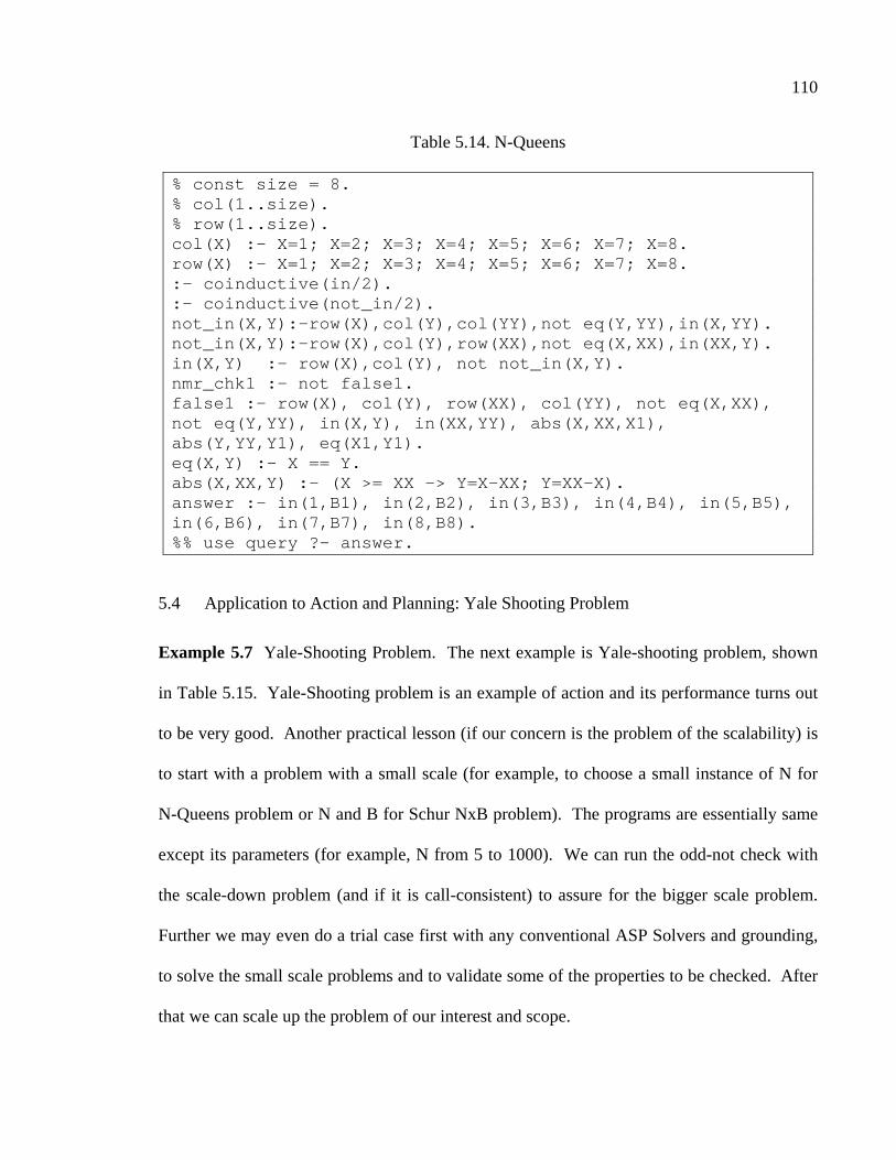
110

Table 5.14. N-Queens

% const size = 8. % col(1..size). % row(1..size). col(X) :- X=1; X=2; X=3; X=4; X=5; X=6; X=7; X=8. row(X) :- X=1; X=2; X=3; X=4; X=5; X=6; X=7; X=8. :- coinductive(in/2). :- coinductive(not_in/2). not_in(X,Y):-row(X),col(Y),col(YY),not eq(Y,YY),in( X,YY). not_in(X,Y):-row(X),col(Y),row(XX),not eq(X,XX),in( XX,Y). in(X,Y) :- row(X),col(Y), not not_in(X,Y). nmr_chk1 :- not false1. false1 :- row(X), col(Y), row(XX), col(YY), not eq( X,XX), not eq(Y,YY), in(X,Y), in(XX,YY), abs(X,XX,X1), abs(Y,YY,Y1), eq(X1,Y1). eq(X,Y) :- X == Y. abs(X,XX,Y) :- (X >= XX -> Y=X-XX; Y=XX-X). answer :- in(1,B1), in(2,B2), in(3,B3), in(4,B4), i n(5,B5), in(6,B6), in(7,B7), in(8,B8). %% use query ?- answer.

5.4 Application to Action and Planning: Yale Shooting Problem

Example 5.7 Yale-Shooting Problem. The next example is Yale-shooting problem, shown

in Table 5.15. Yale-Shooting problem is an example of action and its performance turns out

to be very good. Another practical lesson (if our concern is the problem of the scalability) is

to start with a problem with a small scale (for example, to choose a small instance of N for

N-Queens problem or N and B for Schur NxB problem). The programs are essentially same

except its parameters (for example, N from 5 to 1000). We can run the odd-not check with

the scale-down problem (and if it is call-consistent) to assure for the bigger scale problem.

Further we may even do a trial case first with any conventional ASP Solvers and grounding,

to solve the small scale problems and to validate some of the properties to be checked. After

that we can scale up the problem of our interest and scope.

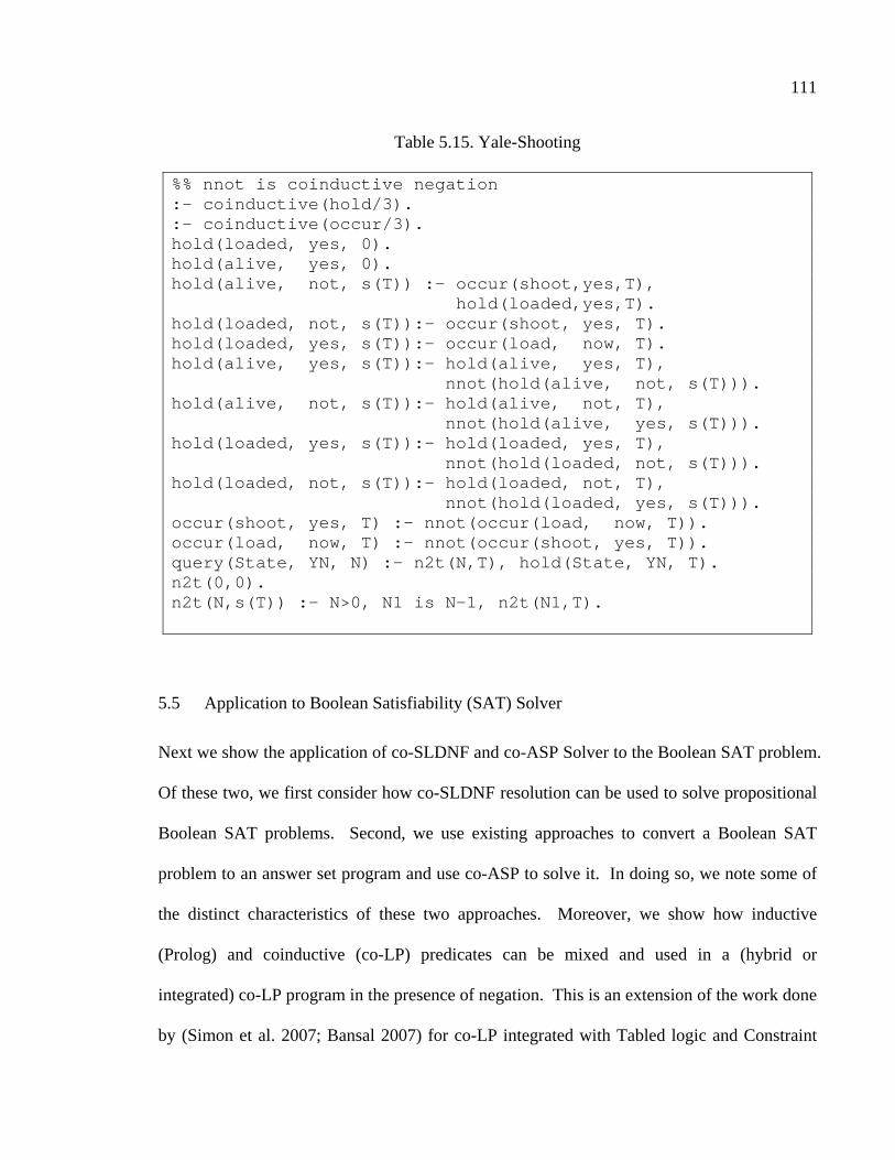
111

Table 5.15. Yale-Shooting

%% nnot is coinductive negation :- coinductive(hold/3). :- coinductive(occur/3). hold(loaded, yes, 0). hold(alive, yes, 0). hold(alive, not, s(T)) :- occur(shoot,yes,T), hold(loaded,yes,T). hold(loaded, not, s(T)):- occur(shoot, yes, T). hold(loaded, yes, s(T)):- occur(load, now, T). hold(alive, yes, s(T)):- hold(alive, yes, T), nnot(hold(alive, not, s( T))). hold(alive, not, s(T)):- hold(alive, not, T), nnot(hold(alive, yes, s( T))). hold(loaded, yes, s(T)):- hold(loaded, yes, T), nnot(hold(loaded, not, s( T))). hold(loaded, not, s(T)):- hold(loaded, not, T), nnot(hold(loaded, yes, s( T))). occur(shoot, yes, T) :- nnot(occur(load, now, T)). occur(load, now, T) :- nnot(occur(shoot, yes, T)). query(State, YN, N) :- n2t(N,T), hold(State, YN, T) . n2t(0,0). n2t(N,s(T)) :- N>0, N1 is N-1, n2t(N1,T).

5.5 Application to Boolean Satisfiability (SAT) Solver

Next we show the application of co-SLDNF and co-ASP Solver to the Boolean SAT problem.

Of these two, we first consider how co-SLDNF resolution can be used to solve propositional

Boolean SAT problems. Second, we use existing approaches to convert a Boolean SAT

problem to an answer set program and use co-ASP to solve it. In doing so, we note some of

the distinct characteristics of these two approaches. Moreover, we show how inductive

(Prolog) and coinductive (co-LP) predicates can be mixed and used in a (hybrid or

integrated) co-LP program in the presence of negation. This is an extension of the work done

by (Simon et al. 2007; Bansal 2007) for co-LP integrated with Tabled logic and Constraint

112

Logic Programming. Note here that (1) we use “not” to denote ASP’s negation as failure, (2)

for coinductive literals we use nt(A) for a negative literal of A in the head of a clause (for

example, { nt(A) :- body. }, and nnot(B) for a negative literal of B occurring in the body of a

clause (for example, { A :- nnot(B), C. }), and (3) for each rule of the form p :- B., its

negated version: nt(p) :- nnot(B) is added during pre-processing. A call nnot( p ) is

evaluated by invoking the procedure for nt(p). Next let us consider the following example of

a simple co-ASP program consisting of two clauses.

Example 5.8 (co-SAT Solver). The following co-LP program is a “naïve” coinductive SAT

solver (co-SAT Solver) for propositional Boolean formulas, consisting of two clauses, as

shown in Table 5.16.

Table 5.16. A naïve Boolean SAT solver BSS1

%% nnot is coinductive negation. :- coinductive(t/1). t(X) :- nnot( neg(t(X)) ). neg(t(X)) :- nnot( t(X) ).

The predicate t/1 is a truth-assignment (or a valuation) where X is a propositional Boolean

formula to be checked for satistifiability. The first clause { t(X) :- nnot( neg(t(X)) ). } asserts

that t(X) is true if there is no counter-case for neg(t(X)) (that is, neg(t(X)) is false

(coinductively), with the assumption that t(X) is true (coinductively)). The second clause {

neg(t(X)) :- nnot( t(X) ). } similarly asserts that neg(t(X)) is true if there is no counter-case

for t(X) . Next, any well-formed propositional Boolean formula constructed from a set of

propositional symbols and logical connectives { ∧, ∨, ¬} and in conjunctive normal form

(CNF) can be translated into a co-LP query for co-SAT program (P1) as follows: First, (1)

113

each propositional symbol p will be transformed into t(p). Second (2), any negated

proposition, that is ¬t(p), will be translated into neg(t(p)). Third (3), for the Boolean

operators, AND (“,” or “∧”) operator will be translated into “,” (Prolog’s AND-operator),

and the OR (or “∨”) operator will be “;” (Prolog’s OR-operator). Note that the “;” operator in

Prolog is syntactic sugar in that “(P ; Q)” is defined as:

P;Q :- P.

P;Q :- Q.

The predicate t(X) determines the truth-assignment of proposition X (if X is true, t(X)

succeeds; else it fails). Note that each query is a Boolean expression whose satistifiability is

to be coinductively determined. Next, we show some of examples of Boolean formulas and

their corresponding co-SAT Boolean queries.

(1) p will be: t(p).

(2) ¬p will be: nnot(t(p)).

(3) p ∧ ¬p will be: t(p) , nnot(t(p)).

(4) p ∨ ¬p will be t(p) ; nnot(t(p)).

(5) p1 ∨ p2 will be: t(p1); t(p2).

(6) p1 ∧ p2 will be: t(p1), t(p2).

(7) ( p1 ∨ p2 ∨ p3 ) ∧ ( p1 ∨ ¬ p3 ) ∧ (¬ p2 ∨ ¬ p4 ) will be: (t(p1); t(p2); t(p3)), (t(p1);

nnot(t(p3))), (nnot(t(p2)); nnot(t(p4))).

Executing the above queries under co-SLDNF will produce a truth assignment in the sets χ+

(positive hypothesis table) and χ- (negative hypothesis table) if the formula is satisfiable.

The above simple SAT solver has been implemented on top of our co-LP system (Gupta et

al. 2007). A built-in called ans has to be added to the end of the query if the user is

114

interested in viewing the truth assignment. Note that we only show the first answer for each

query whereas other models can be found via backtracking.

Table 5.17. Sample Query Results from BSS1

?- t(p1). yes ?- t(p1), neg(t(p1)). no ?- (t(p1); t(p2); t(p3)). yes ?- (t(p1); t(p2); t(p3)),ans. Answer Set: positive_hypo ==> [t(p1)] negative_hypo ==> [ ] yes ?- (t(p), neg(t(p))), ans. no ?- (t(p); neg(t(p))), ans. Answer Set: positive_hypo ==> [t(p)] negative_hypo ==> [ ] yes ?-(t(p1);t(p2);t(p3)),(t(p1); neg(t(p3))), (neg(t(p2)) ; neg(t(p4))), ans. Answer Set: positive_hypo ==> [t(p1)] negative_hypo ==> [t(p2)] yes

The initial performance data of these simple examples is very good and promising toward the

development of a competitive industry-strength co-SAT solver. Next we compare this with

ASP approach and thus how to solve the same problem with co-ASP Solver. Another

115

equivalent but with a minor variation of the “naïve” coinductive SAT solver (co-SAT Solver)

for propositional Boolean formulas is shown in Table 5.18.

Table 5.18. Boolean SAT solver BSS2

pos(X) :- nnot( neg(X) ). neg(X) :- nnot( pos(X) ).

The rules assert that the predicates “pos(X)” and “neg(X)” have mutually exclusive values

(that is, a propositional symbol X cannot be set simultaneously both to true and false).

Thus, the Boolean expression (p1 ∨ p2 ) ∧ ( p1 ∨ ¬ p3 ) ∧ (¬ p2 ∨ ¬ p4 ) will be translated

into the query:

?- (pos(p1);pos(p2)),(pos(p1);neg(p3)),(neg(p2); neg(p4)).

This query can be executed under co-SLDNF resolution to get a consistent assignment for

propositional variables p1 through p4. The assignments will be recorded in the positive and

negative coinductive hypothesis tables (if one were to build an actual SAT solver, then a

primitive will be needed that should be called after the query to print the contents of the two

hypotheses tables). Indeed a meta-interpreter for co-SLDNF resolution has been prototyped

by us and used to implement the naïve SAT solver algorithm. For the query above our system

will print as one of the answers:

positive_hypo ==> [pos(p1), neg(p2)]

negative_hypo ==> [neg(p1), pos(p2)]

The query result outputs the solution where p1 is true and p2 is false. More solutions can be

obtained by backtracking. It is quite interesting to observe how a circular relationship of two

predicates in mutual-negation (for example, pos(X) and neg(X)) could generate a modality

116

with respect to X to be either true or false. Further, it is intellectually stimulating to discover

that even a simpler cyclic program BSS3 shown in Table 5.19.

Table 5.19. Boolean SAT solver BSS3

t(X) :- t(X).

This is yet another Boolean SAT solver with one predicate in a circular relationship of self-

defining or self-referencing. This program would do the same, even more efficiently and

elegantly as the other naïve Boolean SAT solvers could do. In this case, the Boolean

expression (p1 ∨ p2 ) ∧ ( p1 ∨ ¬ p3 ) ∧ (¬ p2 ∨ ¬ p4 ) will be translated into the query:

?- (t(p1); t(p2)), (t(p1); nnot(t(p3))), (nnot(t(p2)); nnot(t(p4))).

Example 5.9 (ASP SAT Solver): As noted in (Baral 2003), propositional logic has been one

of the first languages used for declarative problem solving, specifically for the task of

planning by translating a planning problem into a propositional theory and thus a

satisfiability problem. The following procedure maps a Boolean conjunctive normal form

(CNF) into an answer set program as shown in (Baral 2003).

First (1), for each proposition p in S, let us define p and n_p in P as follows:

p :- not n_p.

n_p :- not p.

Second (2), for each clause ci (that is, i-th clause where 1≤ i ≤ n, for some n clauses in S) and

for each a literal lj (that is, j-th literal occurring in ci), let us define ci as follows:

(2.a) if lj is a positive atom (for example, “a”) then let us define in P: { ci :- lj. }.

(2.b) if lj is a negative atom (for example, “¬a”) then let us define in P: { ci :- n_a. }.

117

Third (3), let us define a headless constraint rule in P for each ci defined in (2) as follows:

:- not ci.

Thus the Boolean CNF formula S of (p1 ∨ p2 ∨ p3 ) ∧ ( p1 ∨ ¬ p3 ) ∧ (¬ p2 ∨ ¬ p4) is

shown in Table 5.20.

Table 5.20. ASP SAT solver of CNF S

%% (p1 ∨ p2 ∨ p3 ) ∧ ( p1 ∨ ¬ p3 ) ∧ ( ¬ p2 ∨ ¬ p4) %% Step (1) p1 :- not n_p1. n_p1 :- not p1. p2 :- not n_p2. n_p2 :- not p2. p3 :- not n_p3. n_p3 :- not p3. p4 :- not n_p4. n_p4 :- not p4. %% Step (2) %% Ste p (3) c1 :- p1. c1 :- p2. c1 :- p3. :- c1. c2 :- p1. c2 :- n_p3. :- c2. c3 :- n_p2. c3 :- n_p4. :- c3.

The corresponding co-ASP P' for the program for P is listed in Table 5.21.

Table 5.21. co-ASP SAT solver of CNF S

%% Step (1) p1 :- nnot n_p1. n_p1 :- nnot p1. p2 :- nnot n_p2. n_p2 :- nnot p2. p3 :- nnot n_p3. n_p3 :- nnot p3. p4 :- nnot n_p4. n_p4 :- nnot p4. %% Step (2) %% Step (3) c1 :- p1. c1 :- p2. c1 :- p3. false1 :- nnot c1 . c2 :- p1. c2 :- n_p3. false2 :- nnot c2. c3 :- n_p2. c3 :- n_p4. false3 :- nnot c3. nmr_chk1 :- nnot false1, nnot false2, nnot false3. %% the query will be ?- nmr_chk1.

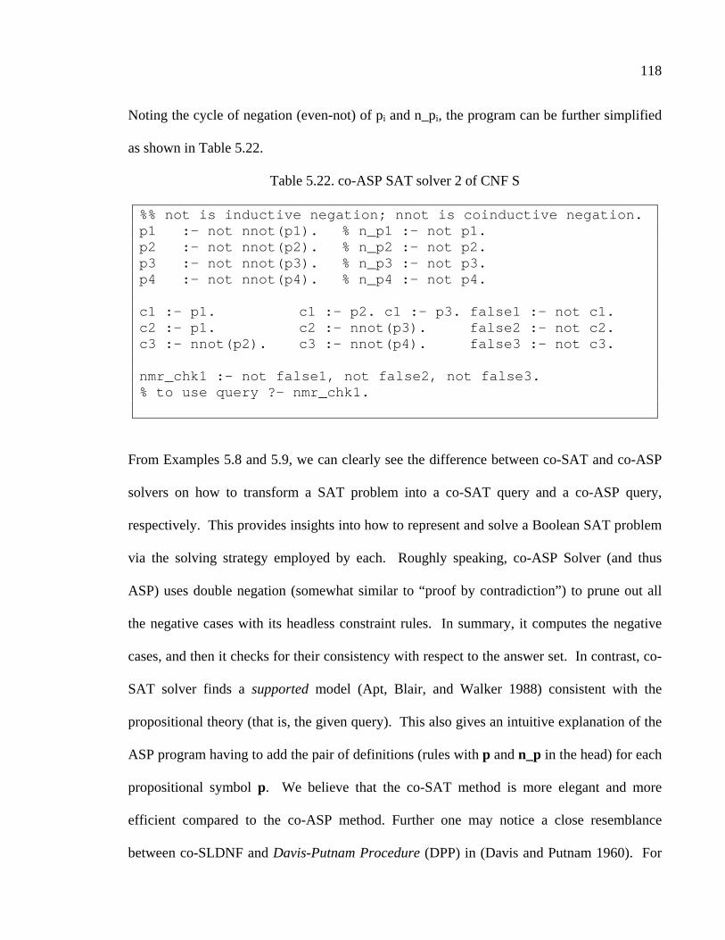
118

Noting the cycle of negation (even-not) of pi and n_pi, the program can be further simplified

as shown in Table 5.22.

Table 5.22. co-ASP SAT solver 2 of CNF S

%% not is inductive negation; nnot is coinductive n egation. p1 :- not nnot(p1). % n_p1 :- not p1. p2 :- not nnot(p2). % n_p2 :- not p2. p3 :- not nnot(p3). % n_p3 :- not p3. p4 :- not nnot(p4). % n_p4 :- not p4. c1 :- p1. c1 :- p2. c1 :- p3. false1 :- not c1. c2 :- p1. c2 :- nnot(p3). false2 :- not c2. c3 :- nnot(p2). c3 :- nnot(p4). false3 :- not c3. nmr_chk1 :- not false1, not false2, not false3. % to use query ?- nmr_chk1.

From Examples 5.8 and 5.9, we can clearly see the difference between co-SAT and co-ASP

solvers on how to transform a SAT problem into a co-SAT query and a co-ASP query,

respectively. This provides insights into how to represent and solve a Boolean SAT problem

via the solving strategy employed by each. Roughly speaking, co-ASP Solver (and thus

ASP) uses double negation (somewhat similar to “proof by contradiction”) to prune out all

the negative cases with its headless constraint rules. In summary, it computes the negative

cases, and then it checks for their consistency with respect to the answer set. In contrast, co-

SAT solver finds a supported model (Apt, Blair, and Walker 1988) consistent with the

propositional theory (that is, the given query). This also gives an intuitive explanation of the

ASP program having to add the pair of definitions (rules with p and n_p in the head) for each

propositional symbol p. We believe that the co-SAT method is more elegant and more

efficient compared to the co-ASP method. Further one may notice a close resemblance

between co-SLDNF and Davis-Putnam Procedure (DPP) in (Davis and Putnam 1960). For

119

example, consider the CNF formula, (p) ∧ (p ∨ q) ∧ (¬ p ∨ r), consisting of three clauses. If

p is true (a stand-alone clause), in DPP, Clauses 1 and 2 will disappear and Clause 3 will be

left with (r) after deleting (¬¬¬¬ p). In co-SAT, p is true; thus Clauses 1 and 2 will be empty

clauses, and Clause 3 will be evaluated for r (as not p is false). DPP has a few more rules

including splitting to check whether p is true or p is false (to try either cases) whereas co-

SAT accomplishes the same with backtracking.

Example 5.10 (Predicate Boolean SAT). In this example, we extend our application of co-

LP to first order queries and quantified (Boolean) formulas as noted in [6]. Note that here we

follow the order of the presentation and the notations found in [6]. First, let us elaborate on

closed first-order queries in ASP, and thus to co-LP and co-ASP Solver. Let F1 and F2 be

closed Boolean formulas and pF1 and pF2 be the corresponding predicates, respectively. The

translation rules are similar to what we note in Example 5.8.

(1) AND: the formula F=(F1 ∧ F2) is translated into the following rule: { pF :- pF1, pF2.}.

(2) OR: the formula F=(F1 ∨ F2) is translated into the following rule: { pF :- pF1; pF2. } or

two following rules: { pF :- pF1. pF :- pF2. }.

(3) NOT: the formula F=(¬F1) is translated into the following rule: { pF :- nt(pF1).}.

(4) Existential Quantifier: the formula F=(∃X.F1(X)) is translated into the following rule: {

pF :- pF1(X). }.

(5) Bounded Existential Quantifier: the formula F=(∃X.(F1(X)→F2(X)) is translated into the

following rule: { pF :- pF1(X), pF1(X).} or the rule using Prolog (if-then): { pF :-

pF1(X) −−−−>>>> pF1(X).}.

120

(6) Universal Quantifier: the formula F=(∀X.(F1(X)) is translated into the following rule: {

pF :- not nt(pF1(X)). }, or two rules: { pF :- nt(n_pF). n_pF :- nt(pF1(X)).}.

(7) Bounded Universal Quantifier: the formula F=(∀X.(F1(X) → F2(X))) is translated into

the following rule: { pF :- not (pF1(X), nt(pF2(X))). }, or two rules: { pF :- nt(n_pF).

n_pF :- pF1(X), nt(pF2(X)).}.

Next, we explore and extend our work on co-LP with co-SLDNF resolution for its

applications to rational sequences, ω-automata, model checking in Linear Temporal Logic

(LTL) and Computation Tree Logic (CTL) (Baier and Katoen 2008; Clarke 1999; Huth and

Ryan 2004). Further we present an implementation of a naïve coinductive LTL solver (co-

LTL solver) and a naïve coinductive CTL solver (co-CTL solver), and correctness results.

First we define the semantics of LTL modeled as a transition system by means of states and

transitions (Huth and Ryan 2004).

5.6 Rational Sequences

A transition system TS (also called a model) is a 4-tuple of <S, T, A, L> where (a) S is a set

of a finite states, (b) T is a set of binary transition relation where if s in S and s′ in S then a

transition t(s, s′) in T defines a transition from s to s′ denoted { s → s′ }, (c) A is a set of

atoms where an atom a (or its negation, ¬a) in A may be associated with a state s in S, (d) via

labeling function L where L maps an atom a to the truth value (true or false) for each state s.

This is a simplified TS without Action or Event or final states, compared to a classical 5-

tuple TS. A sequence I of state-transition of TS is denoted by I = [s1, s2, s3, …] of states

starting from a state s1 in S, and each transition (si, si+1) is well-defined. We denote Ii for the

suffix of I starting at si (for example, I2 = [s2, s3, …].

121

As we noted earlier, a tree can be defined recursively as follows: Let node(A, L) be a

constructor of a tree where A is a node and L is a tree. A rational tree (denotes RT) is a tree

where the set of all of its subtrees is finite. (We may note that this notation of node(A,L) is

equivalent to “(A . L)” or “ . (A, L)” in dot-notation, or “[A | L]” in list-notation. A rational

sequence (denotes RS) is a rational tree where each A of node(A, L) is a leaf of atom. A

rational sequence is formed when L of node(A, L) is one of its preceding nodes. Moreover, a

rational sequence can be represented by its minimal and unique canonical representation of

rational tree. For example, X = [s1, s2 | X] is a rational sequence containing a cyclic sequence

of {s1, s2}. Consider X=[s0], Y=[s1, s2 | Y], and Z=[X, Y]. The canonical representation of

X, Y and Z is then [s0], [{s1, s2}], and [s0, {s1, s2}], respectively. The length of each

canonical representation is the length of its finite prefix-subsequence plus the length of its

suffix cyclic-subsequence. Thus the length of the canonical representation of X, Y, and Z is

1, 2, and 3, respectively. The maximum length of the canonical representation of a rational

sequence is less than or equal to the cardinality of the set of the states S. Thus, given a

rational sequence I = [s1, ..., si, si+1, ..., sm, sm+1, …] where n is the cardinality of S, let sm+1 be

the first repeating state symbol (that is, sm+1=si+1) of a cycle { si+1, ..., sm }. Then recurring

sm+1 signifies the presence of cycle {si+1, ..., sm} along with its finite prefix subsequence of

[s1, ..., si] where i ≤ m ≤ n. Therefore it is sufficient to test at most first (n+1) state symbols

of a rational sequence to decide its canonical representation, to decide its finite-prefix and its

cycle-suffix. Similarly one may also represent a rational tree (a system of equations) with ω-

regular expression of a finite prefix followed by a cyclic-suffix.

An ω-regular expression can be expressed with a set of rational trees. Consider an ω-

regular expression J = E1F1ωE2F2

ω … EnFnω where Ei is a finite prefix string and Fi

ω is a

122

cyclic string (that is, Fiω is a possibly infinite repetition of a finite string Fi) where 1 ≤ i ≤ n.

Further Fi can be divided into two parts of GiHi where Gi is the prefix string to be taken when

a cycle of F1 is not taken. Then J can be expressed with n rational sequences of [E1{F1}],

[E1G1E2{F2}], …, [E1G1E2G2 … En{Fn}] in canonical representation. For example, consider

an example of a ω-automaton and its ω-string J1, shown in Figure 5.5.

Figure 5.5. J2= (ab)(cdef)ω(g)(hijk)ω

Then J1 = E1F1ω where E1 = (ab) and F1 = (cdefgh) and further G1=(cde) and H1=(fgh). The

canonic representation is [ab{cdefgh}]. Consider another example of an ω-automaton and its

ω-string J2, shown in Figure 5.6.

Figure 5.6. J2= (ab)(cdef)ω(g)(hijk)ω

a b c d g

k e f

h i

j

J2= (ab)(cdef)ω(g)(hijk)ω

a b c d e

f g h

J1=(ab)(cdefgh)ω

123

Then J2 = E1F1ω E2F2

ω where E1 = (ab), F1 = (cdef), G1 = (cd), H1 = (ef), E2 = (g), F2 = (hijk),

G2 = (hi), and H2 = (jk). Its canonic representation is [ab{cdef}], [abcdg{hijk}].

Example 5.11 Let us consider an ω-automaton A1, shown in Figure 5.7.

Figure 5.7. Example of ω-Automaton - A1

The ω-automaton A1 consists of 4 states, { s0, s1, s2, s3 }, and 6 events, {bootup, work,

crash/off, shutdown, booterror, reboot}. This example models the operation of a computer.

The corresponding co-LP program code that models the automaton is shown in Table 5.23:

Table 5.23. co-LP for A1

:- coinductive(state/2). state(s0,[s0|T]) :- event(bootup), state(s1,T). state(s1,[s1|T]) :- event(work), state(s1,T). state(s1,[s1|T]) :- event(crash/off), state(s2,T). state(s2,[s2|T]) :- event(shutdown), state(s0,T). state(s0,[s0|T]) :- event(booterror), state(s3,T). state(s3,[s3|T]) :- event(reboot), state(s0,T). event(bootup). event(work). event(crash/off). event(shutdown). event(booterror). event(reboot).

crash/off shutdown

bootup work

bootup reboot

s0 s1

s3 s2

124

The query ?- state(S,T) generates all the possible rational paths in canonical representation,

each ending with a cycle whereas the query ?- state(X,T), X=s0 will narrow the results to

cycles, starting from the initial state s0.

T = [s0,s1,s1,s1,s1,s1,s1,s1,s1,s1,...];

T = [s0,s1,s2,s0,s1,s2,s0,s1,s2,s0,...];

T = [s0,s,s0,s3,s0,s3,s0,s3,s0,s3,...]

As it is shown here, the coding of the automata is intuitively simple and self-explanatory.

The cycle (the states in cycle being repeated) is underlined for the reader. All the infinite

sequences generated are the rational sequences where each has one and only one cycle at the

end of its sequence, in the canonical representation. This is one advantage of co-LP in

dealing with rational sequences, to enable one to generate all the rational sequences in the

canonical representation. These examples demonstrate the generative capability of co-LP

with respect to rational sequence in the canonical representation. Further its capability is not

restricted to the rational sequences in the canonical representation only. Any finite and

rational sequences can be checked by the query. For example, the rational sequence of

[s0,s1,s1,s2,s0,s1,s1,s1,…] can be easily checked by the query ?- X=[s1|X],

Y=[s0,s1,s1,s2,s0,X], state(s0,Y). Next, let us consider the query ?-state(X,T), nt(state(s0,

T)). The query result shows all the cycles that do not start with s0.

T = [s1,s1,s1,s1,s1,s1,s1,s1,s1,s1,...];

T = [s1,s2,s0,s1,s2,s0,s1,s2,s0,s1,...];

T = [s1,s2,s0,s3,s0,s3,s0,s3,s0,s3,...];

T = [s2,s0,s1,s1,s1,s1,s1,s1,s1,s1,...];

T = [s2,s0,s1,s2,s0,s1,s2,s0,s1,s2,...];

125

T = [s2,s0,s3,s0,s3,s0,s3,s0,s3,s0,...];

T = [s3,s0,s1,s1,s1,s1,s1,s1,s1,s1,...];

T = [s3,s0,s1,s2,s0,s1,s2,s0,s1,s2,...];

T = [s3,s0,s3,s0,s3,s0,s3,s0,s3,s0,...]

Thus a query ?- state(S,T) may generate all the possible rational paths in the canonical

representation of a TS defined above, each ending with a cycle (affix-cycle sequence) if it is

a rational sequence, and all via co-SLDNF resolution. Further one may define a set of final

states F as facts so that, when a transition reaches this state, co-SLDNF resolution will

terminate as a successful (finite) derivation. Alternatively one may define a cycle to a state

A to itself so that once a transition reaches this state it terminates as a successful derivation.

For example, consider s2 as a final state defined in two ways:

(a) state(s2,[s2|T]).

(b) state(s2,[s2|T]) :- state(s2,T)

These examples show the applications of co-LP (Simon et al. 2007) to ω-automata and ω-

regular expressions with more examples available in (Min and Gupta 2008b). Next, we

explore the application of co-LP and rational sequences to model checking towards model

checking (Baier and Katoen 2008; Clarke 1999). We present LTL followed by CTL,

modeled as a transition system.

5.7 Coinductive LTL Solver

First we present the syntax of LTL in BNF found in (Huth and Ryan 2004) as follows:

Definition 5.1 (Syntax and semantics of LTL):

φ ::= true | false | p | (¬φ) | (φ ∧ φ) | (φ ∨ φ) | (φ → φ)

126

| (X φ) | (G φ) | (F φ) | (φ U φ) | (φ W φ) | (φ R φ)

where φ is an LTL formula, p is any propositional atom in A of TS with the logical

connectives LC={ ¬, ∧, ∨, → } as defined in propositional logic and the temporal

connectives TC={X, F, G, U, W, R} defined as follows: Let M = <S, T, A, L> be a transition

system and I = [s1, s2, s3, …] be a path in M. Then I satisfies an LTL formula φ is defined by

the satisfaction relation (denoted |=) as follows:

(1) I |= true.

(2) I |≠ false

(3) I |= p iff p ∈ L(s1)

(4) I |= ¬φ iff I |≠ φ

(5) I |= (φ1 ∧ φ2) iff I |= φ1 and I |= φ2

(6) I |= (φ1 ∨ φ2) iff I |= φ1 or I |= φ2

(7) I |= (φ1 → φ2) iff I |= φ2 whenever I |= φ1

(8) I |= (X φ) iff I 2 |= φ

(9) I |= (G φ) iff ∀i ≥ 1, Ii |= φ

(10) I |= (F φ) iff ∃ i ≥ 1, Ii |= φ

(11) I |= (φ U ψ) iff ∃ i ≥ 1, Ii |= ψ and ∀ j = 1, …, i-1, Ij |= φ

(12) I |= (φ W ψ) iff (∃ i ≥ 1, Ii |= ψ and ∀j = 1, …, i-1, Ij |= φ) or (∀k ≥ 1, Ik |= φ)

(13) I |= (φ R ψ) iff (∃ i ≥ 1, Ii |= φ and ∀j = 1, …, i-1, Ij |= ψ) or (∀k ≥ 1, Ik |= ψ).

A naïve co-LTL Solver is defined in Table 5.24. Note that each LTL connective in LC={ ¬,

∧, ∨, → } is coded as { “not”, “,”, “;”, “->” }, respectively and each in the temporal LTL

127

connectives, TC={ X, F, G, U, W, R }, are coded {next, future, global, until, weak-until,

release}, respectively.

Table 5.24. A naïve co-LTL Solver

%% naïve co-LTL solver %% note 1 - valid/2 is coinductive. note 2 - op(S) is atomic_prop(S). valid(Path,true). %% 1 - True valid(Path,false) :- fail. %% 2 - False valid([S|P],L) :- op(S), label(S,L). %% 3 - label valid([S|P],(not L)):- op(S), label(S, L), fail. %% 4 - not valid([S|P],(not L)):- op(S), label(S1,L), not label(S,L). valid([S|P],(not L)):- op(S), not valid([S|P],L). valid([S|P],(L1,L2)):-(valid([S|P],L1), valid([S|P],L2)). %% 5 - and valid([S|P],(L1;L2)):-(valid([S|P],L1); valid([S|P],L2)). %% 6 - or valid([S|P],(L1 -> L2)):-(valid([S|P],L1) -> valid([S|P],L2); true). %% 7 - if valid([S1, S2|P], next(L)) :- valid([S2|P], L). %% 8 - next %% --- 9 global - for every states in Path (cyclic list). valid([S|P], global(L)):-valid([S|P],L), ck_gs(P,L,[S]). ck_gs([],L,H). %% for finite path ck_gs([S|P],L,H) :- member(S, H). ck_gs([S|P],L,H) :- valid([S|P],L), ck_gs(P,L,[S|H]). %% --- 10 future valid([S|P],future(L)) :- (valid([S|P],L) ; ch_fstate(P,L,[S])). ch_fstate([],L,H) :- fail. ch_fstate([S|P],L,H) :- member(S, H) -> fail; (valid([S|P],L); ch_fstate(P,L,[S|H])). %% --- 11 until valid(P,until(A,B)):-valid(P,A), state_list(Sl), length(Sl,N), M is 2*N,get_ns(P, M,Ss),Ss=[S1|P1], ck_u(P1,until(A,B)). ck_u(Path,until(A,B)) :- valid(Path,B). ck_u([],until(A,B)) :- fail. ck_u([S|Path],until(A,B)) :- valid([S|Path],A), ck_u(Path,until(A,B)). get_ns(P,N,Ss) :- get_ns(P, N, [], R), reverse(R,Ss). get_ns(Path,0,Result,Result). get_ns([],N,Result,Result). get_ns(Path,N,States,Result) :- N>0, N1 is (N-1), Path=[S|Path1], get_ns(Path1,N1,[S|States],Result). %% --- 12 weakuntil valid([S|P],weakuntil(A,B)) :- valid([S|P], until(A,B)). valid([S|P],weakuntil(A,B)) :- valid([S|P], global(A)). %% --- 13 release valid([S|P],release(A,B)) :- valid([S|P], weakuntil(B,A)). member(X,[X | _]). member(X,[_ | Y]) :- member(X,Y).

128

As discussed earlier, we use co-LP to enumerate all the (finite and rational) paths in

canonical representation (of the states of the state-transition system). The solver maintains a

list of state for F (future) operator to check whether the current state has been encountered

previously, in order to detect a cycle (of a canonical representation where any rational

sequence has its one and only one cycle as suffix).

Next, we present the correctness of co-LTL solver. The sketch of the proof is based

on the following observations. As noted earlier, there are a finite number of rational

sequences with suffix-cycle of a co-TS, and that a query ?- state(IS,SP) with co-SLDNF

enumerates all of the paths of both finite sequences and rational sequences with suffix-cycle.

Each state s in S will be selected for IS and the query with co-SLDNF resolution traverses

the transition rules to generate a path which is to be terminated when it hits a leaf node (a

fact) or when it detects a cycle (by coinductive proof). Then it does backtracking to pick up

next state or next transition to be explored (similar to a topological ordering of a graph).

Due to co-SLDNF resolution, it keeps track of all the nodes in the current path, to detect a

cycle to be terminated if recurring. As a result, we have the soundness of co-LTL solver.

For the completeness of co-LTL solver, we note that there is no other way to construct LTL

formula other than the well-defined LTL formula recursively defined as in Definition 5.1

where each LTL formula is finite in length and processed recursively (with structural

induction) accordingly by co-LTL solver (and thus this is the proof for completeness of co-

LTL solver). Therefore we have the following correctness results in somewhat informal

manner. First (1), given a co-TS, a query ?- state(S,T) with co-SLDNF resolution will find

and enumerate all the paths of finite sequences and rational sequences with cycle at end.

Moreover the number of all the paths enumerated is finite. Second (2), since each path is

129

either a finite sequence or a rational sequence with cycle at end, the number of the states to

be checked for of each path is finite (that is, n+1 as an upper bound where |S|=n) and the

order of the states in the path is well-defined and deterministic. Third (3), for each state of

each path, to test the satisfaction relation for each of LTL formula φ defined in Definition

5.1 is well-defined and (finitely) decidable by co-LTL solver (Soundness of co-LTL solver).

Finally (4), co-LTL solver solves only a (syntactically) well-defined class of formula φ which

is a well-defined finite LTL formula. That is, there is no other finite LTL formula that co-

LTL solver cannot decide its validity by structural induction. This concludes for the

completeness of co-LTL solver.

Theorem 5.1 (Soundness and Completeness of co-LTL Solver). Given a LTL formula φ,

I |=co-LTL φ iff I |=LTL φ.

Example 5.12 Let us consider another simple example of an automaton A2 shown in Figure

5.8 (Huth and Ryan 2004), consisting of three states {s0, s1, s2} and its internal labeling (or

content) for each state, to illustrate co-LTL solver.

Figure 5.8. An example of ω-Automaton A2

q,r

p,q

r

s0

s1 s2

130

The co-LP implementation of this an ω-automaton is shown in Table 5.25. Co-LP A2.

Table 5.25. Co-LP A2

:- coinductive(state/2). state_list([s0, s1, s2]). state(s0,[s0|T]):-state(s1,T). state(s0,[s0|T]):-state(s2,T). state(s1,[s1|T]):-state(s0,T). state(s1,[s1|T]):-state(s2,T). state(s2,[s2|T]):-state(s2,T). label(s0,p). label(s0,q). label(s1,q). label(s1,r). label(s2,r).

Some of the queries to test the validity of co-LTL Solver for the example are shown in Table

5.26. First query ?- state(s0,P), valid(P, global(p)) checks all the paths starting from the

state s0, for the validity of the formula, global(p).

Table 5.26. Co-LP A2 Sample Queries

?- state(s0,P),valid(P,global(p)). No

?- state(s0,P),valid(P,global(q)). P = [s0,s1,s0,s1,s0,s1,s0,s1,s0,s1,...] ? yes

?- state(s0,P),valid(P,future(p)).

P = [s0,s1,s0,s1,s0,s1,s0,s1,s0,s1,...] ? yes

?- state(s2,P),valid(P,future(p)).

no ?- state(s0,P),valid(P,until(p)).

no ?- state(s0,P),valid(P,until(p,q)).

P = [s0,s1,s0,s1,s0,s1,s0,s1,s0,s1,...] ? yes

131

5.8 Coinductive CTL Solver

First we present the syntax of CTL in BNF found in (Huth and Ryan 2007) as follows:

Definition 5.2 (Syntax and semantics of CTL):

φ ::= true | false | p | (¬φ) | (φ ∧ φ) | (φ ∨ φ) | (φ → φ) | (AX φ) | (EX φ) | (AF φ) | (EF φ)

| (AG φ) | (EG φ) | (A(φ U φ)) | (E(φ U φ))

where φ is a CTL formula, p is any propositional atom in A of TS with the logical

connectives LC={ ¬, ∧, ∨, → } as defined in propositional logic and the temporal

connectives TC={X, F, G, U} with the path Modal operator {A, E} meaning {“along all

paths” , “along at least one path”, respectively. The semantics of CTL is defined as follows:

Let M = <S, T, A, L> be a transition system and s be a state in S, and let I = [s1, s2, s3, …] be

a valid path where s=s1. Then the state s satisfies a CTL formula φ is defined by the

satisfaction relation (denoted |=) as follows:

(1) s |= true.

(2) s |≠ false

(3) s |= p iff p ∈ L(s)

(4) s |= ¬φ iff s |≠ φ

(5) s |= (φ1 ∧ φ2) iff s |= φ1 and s |= φ2

(6) s |= (φ1 ∨ φ2) iff s |= φ1 or s |= φ2

(7) s |= (φ1 → φ2) iff s |= φ2 whenever s |= φ1

(8a) s |= (AX φ) iff for all si such that s → si, si |= φ

(8b) s |= (EX φ) iff for some si such that s → si, si |= φ

132

(9a) s |= (AG φ) iff for all paths s1 → s2 → s3 → …, where s1 = s, and all si along the path,

si |= φ, and (9b) s |= (EG φ) iff there is a path s1 → s2 → s3 → …, where s1 = s, and

some si along the path, si |= φ

(10a) s |= (AF φ) iff for all paths s1 → s2 → s3 → …, where s1 = s, and some si along with

path, si |= φ, and (10b) s |= (EF φ) iff there is a path s1 → s2 → s3 → …, where s1 = s,

and some si along the path, si |= φ

(11a) s |= A(φ U ψ) iff for all paths s1 → s2 → s3 → …, where s1 = s, and that path satisfies φ

U ψ, and (11b) s |= E(φ U ψ) iff there is a path s1 → s2 → s3 → …, where s1 = s, and

that path satisfies φ U ψ.

The implementation of a naïve co-CTL solver is again straightforward and shown in Table

5.27.

Table 5.27. A naïve co-CTL Solver

%% 1 & 2 - True & False valid(State,true) :- label(State,_). valid(State,false):- label(State,_), fail. %% 3 - Literal valid(State,L) :- label(State,L). %% 4 - NOT valid(State, (not L)) :- label(State, L), fail. valid(State, (not L)) :- label(S,L), not label(State, L). valid(State, (not L)) :- not valid(State,(L)). %% 5 - AND valid(State,(L1,L2)) :- (valid(State,L1), valid(State,L2)). %% 6 - OR valid(State,(L1; L2)) :- (valid(State,L1); valid(State,L2)). %% 7 - -> valid(State,(L1 -> L2)) :- (valid(State,L1) -> valid(State,L2)). %% 8 - next valid(State, next(L)):-state(State,[State,S2|Path]), valid(S2,L). %% 9a - allglobal - for every states in all Paths (cyclic list). valid(S,allglobal(L)):-setof(P,state(S,P),Ps),ckgl(S,Ps,L). ckgl(S,[],L).

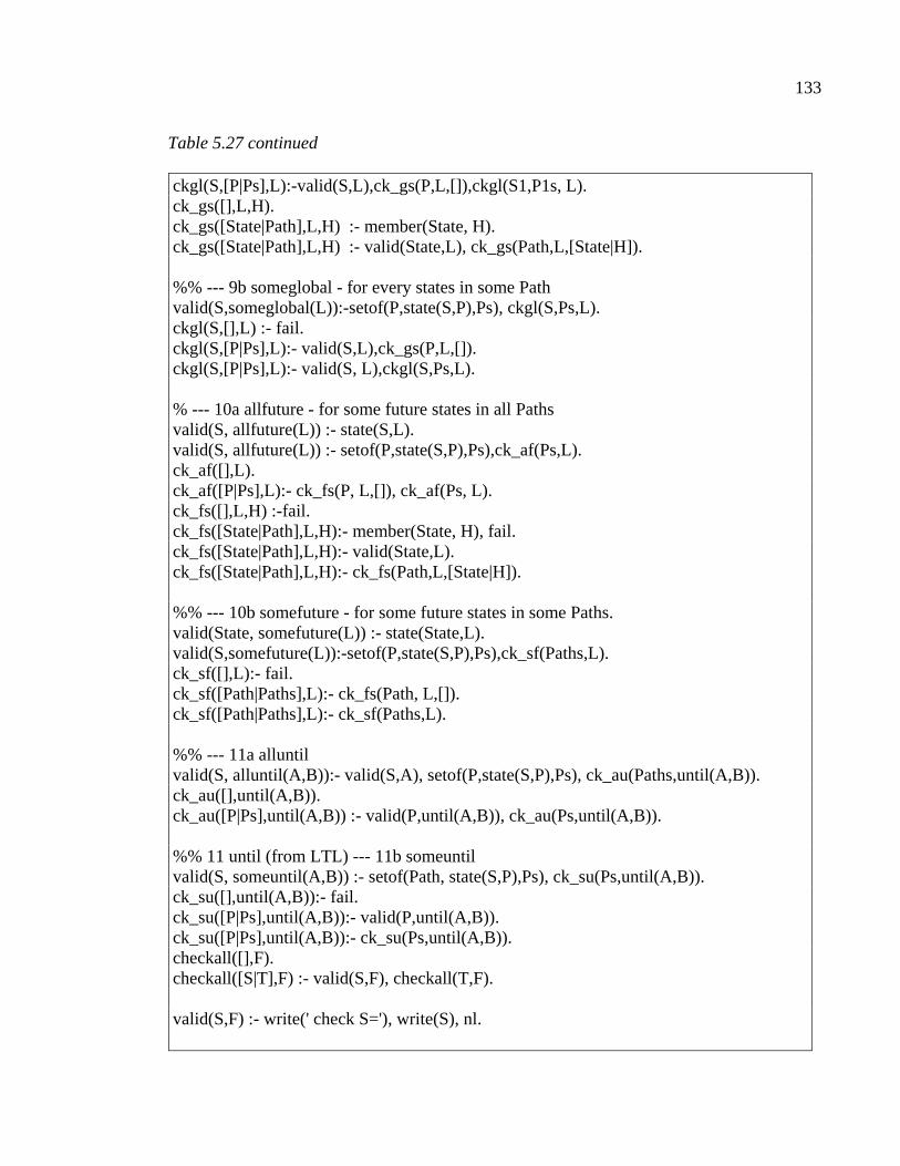
133

Table 5.27 continued

ckgl(S,[P|Ps],L):-valid(S,L),ck_gs(P,L,[]),ckgl(S1,P1s, L). ck_gs([],L,H). ck_gs([State|Path],L,H) :- member(State, H). ck_gs([State|Path],L,H) :- valid(State,L), ck_gs(Path,L,[State|H]). %% --- 9b someglobal - for every states in some Path valid(S,someglobal(L)):-setof(P,state(S,P),Ps), ckgl(S,Ps,L). ckgl(S,[],L) :- fail. ckgl(S,[P|Ps],L):- valid(S,L),ck_gs(P,L,[]). ckgl(S,[P|Ps],L):- valid(S, L),ckgl(S,Ps,L). % --- 10a allfuture - for some future states in all Paths valid(S, allfuture(L)) :- state(S,L). valid(S, allfuture(L)) :- setof(P,state(S,P),Ps),ck_af(Ps,L). ck_af([],L). ck_af([P|Ps],L):- ck_fs(P, L,[]), ck_af(Ps, L). ck_fs([],L,H) :-fail. ck_fs([State|Path],L,H):- member(State, H), fail. ck_fs([State|Path],L,H):- valid(State,L). ck_fs([State|Path],L,H):- ck_fs(Path,L,[State|H]). %% --- 10b somefuture - for some future states in some Paths. valid(State, somefuture(L)) :- state(State,L). valid(S,somefuture(L)):-setof(P,state(S,P),Ps),ck_sf(Paths,L). ck_sf([],L):- fail. ck_sf([Path|Paths],L):- ck_fs(Path, L,[]). ck_sf([Path|Paths],L):- ck_sf(Paths,L). %% --- 11a alluntil valid(S, alluntil(A,B)):- valid(S,A), setof(P,state(S,P),Ps), ck_au(Paths,until(A,B)). ck_au([],until(A,B)). ck_au([P|Ps],until(A,B)) :- valid(P,until(A,B)), ck_au(Ps,until(A,B)). %% 11 until (from LTL) --- 11b someuntil valid(S, someuntil(A,B)) :- setof(Path, state(S,P),Ps), ck_su(Ps,until(A,B)). ck_su([],until(A,B)):- fail. ck_su([P|Ps],until(A,B)):- valid(P,until(A,B)). ck_su([P|Ps],until(A,B)):- ck_su(Ps,until(A,B)). checkall([],F). checkall([S|T],F) :- valid(S,F), checkall(T,F). valid(S,F) :- write(' check S='), write(S), nl.

134

Next we present the correctness of co-CTL solver. The sketch of the proof is very similar to

that of co-LTL solver, as we note that there are a finite number of rational sequences that can

be effectively generated and enumerated for checking of each CTL formulas, and thus the

enumeration of each state within a path to be tested for CTL formula. Second we note that

there is no other way to construct CTL formula other than the well-defined CTL formula,

which is finite in length, recursively defined as in Definition 5.2 where each CTL formula is

processed recursively accordingly by co-LTL solver with structural induction (and this is for

the completeness of co-LTL solver). Thus we have the following proof of the correctness

result.

Given a co-TS M, (1) there is an effective way to enumerate all the states and all the

paths of M. Further the number of all the paths enumerated is finite as well as the number of

the states. (2) Since each path is either a finite sequence or a rational sequence with cycle at

end, the number of the states of each path is finite (that is, n+1 as an upper bound where

|S|=n) and the order of the states in the path is well-defined and deterministic. (3) Thus for

each state of each path, to test the satisfaction relation for each of CTL formula φ defined in

Definition 5.2 is well-defined and finitely decidable by co-CTL solver (Soundness of co-CTL

solver). (4) Further co-CTL solver solves only a (syntactically) well-defined class of formula

φ which is a well-defined finite CTL formula. That is, there is no other finite CTL formula

that co-CTL solver cannot decide its validity with structural induction (Completeness of co-

CTL solver).

Theorem 5.2 (Soundness and Completeness of co-CTL Solver). Given a CTL formula φ,

I |=co-CTL φ iff I |=CTL φ.

135

By combining co-LTL solver for paths and co-CTL solver for states, one may construct

coinductive CTL* (co-CTL*) solver in a straightforward manner. Further one may note that

it is straightforward to extend propositional LTL and CTL to predicate LTL and CTL by

allowing the formula with variables. For example, the property p in the example of ω-

Automaton A2 in Figure 5.8 can be defined as a predicate p(X) where it is defined as a rule

(for example, as a constraint), with a query ?- state(s0,Path), valid(Path, global(p(X))).

label(s0, p(X)) :- p(X).

p(X) :- X >= 0, X < 2**64.

Thus if we consider the number of states (for example, 1020 which can be easily reached with

80 Boolean properties for 280 = 1620 > 1020), the potential of predicate LTL and CTL solvers

is significant in our belief. We note also that the performance of our prototype

implementation is not comparable to those systems of model checking (for example, SMV4,

nuSMV5, and SPIN6). Further, a minor variation in TS can provide a powerful tool for path

analysis of a graph dealing with infinite cycle, for predicate dependency graph and path

analysis. For example, let us consider state/2 predicate (for example, a state transition from

s0 to s1) to be defined as follows:

state(s0, [(s0, sign)|T]) :- state(s1,T).

where sign is “+” if a transition from s0 to s1 is positive or “-” if negative, to express an

answer set program as a predicate dependency graph. The corresponding predicate

dependency relations are defined as follows:

4 http://www.cs.cmu.edu/~modelcheck/

5 http://nusmv.irst.itc.it/

6 http://spinroot.com/spin/whatispin.html

136

state( Lo , [(Lo , +) | T] ) :- state(Li , T).

state( Lo , [(Lo , -) | T] ) :- state(Lj , T).

where 1 ≤ i ≤ m, and m+1 ≤ j ≤ n. As we noted earlier for co-ASP solver, one of the critical

tasks in solving predicate ASP program deals with the integrity check to detect any odd-cycle

rule for consistency (that is, call-consistency).

137

CHAPTER 6

PERFORMANCE AND BENCHMARK

6.1 Introduction

Most of the small ASP examples and their queries run very fast (usually under 0.0001 CPU

Seconds) as we noted earlier on Linux system in a shared environment with Dual Core AMD

Opteron Processor 275, with 2GHz with 8GB memory, running on YAP Prolog1 with a stack

size of 20MB. Thus we selected three well-known programs (Schur, N-Queens and Yale

Shoot problems) for its performance and benchmark (Dovier, Formisano, and Pontelli. 2005;

Bonatti, Pontelli, and Son. 2008) which is available, well-studied in ASP and Constraint

Logic Programming (CLP), and in Prolog, and done with a comparable hardware

configuration that we are using. In general, co-ASP Solver is doing well with simple ASP

programs without the constraint rules and integrity check, comparable to the performance of

ASP Solvers such as Smodel. For constraint satisfaction problems like Schur numbers and

N-Queen problems, ASP solvers are doing much better than co-ASP Solver which is also

getting slower as the problem size gets bigger. We believe that this is due to how the

constraint rules are being handled by co-ASP Solver currently without memory. That is, co-

ASP Solver repeats the same computation over and over for each constraint rule is computed.

In contrast, co-ASP Solver does outperformed for Yale-Shooting problem over ASP Solvers

as the size of the time-duration T gets larger and larger, and finished with 0.0001 CPU

1 http://www.dcc.fc.up.pt/~vsc/Yap/

138

second especially for Alive = No for T=2000, while Smodels is timed out (after 1 CPU hour)

even for T = 100.

As noted earlier, the performance and benchmark of co-ASP Solver is yet premature,

as compared with its counterparts (for example, ASP Solvers, SAT Solvers, and CLP

Solvers). However the results are very promising. Current stage of co-ASP Solver and its

prototype is still at the early stage of experimentation. Thus we believe that current co-ASP

Solver still have a long way for its development cycle, comparing with the matured

mainstream ASP Solvers, SAT Solvers or CLP Solvers in their product and development

cycle. However, the initial performance results are very promising considering a few factors.

First (1), co-ASP Solver is solving predicate ASP program, almost as it is given, without

grounding. And this would be the major advantage of co-ASP Solver, if grounding becomes

a major bottleneck for current ASP Solvers. Second (2), current co-ASP Solver is solving

ASP program in a naïve mode, contrast to current ASP Solvers fully equipped with rich and

intelligent heuristics and problem-solving strategies. Thus there seems a lot of room for co-

ASP Solver to grow and improve itself for its performance and competitive edge, and in

tuning and optimization. Further, co-ASP Solver provides an alternative strategy for current

ASP Solvers or toward the development of a hybrid ASP Solver, combining the best of these

two paradigms (bottom-up and top-down). In addition, co-ASP Solver provides an

alternative semantics of partial/total model and gfp/lfp, extending its language specification

into the fully-functional predicate language including arbitrary function symbols and fixed

point of infinity (for example, X=f(X)). With co-SLDNF, co-ASP programming language is

now powerful enough to compute and model infinite objects and streams within the scope of

rationality.

6.2

Sc

(Table

placed in the 5 boxes and we are merely checking that the constrai

the co

all 12 numbers in the 5 boxes provided subject to constraints). The second case (

Fig

B=5.

6.2 Schur Number

Schur 5x12 is tested with various queries which include partial solutions of various lengths I

(Table 6.1; Figure 6.1

placed in the 5 boxes and we are merely checking that the constrai

the co-ASP Solver searches

all 12 numbers in the 5 boxes provided subject to constraints). The second case (

Figure 5.2) is the gen

B=5.

Schur 5x12

CPU sec.

Schur Number

is tested with various queries which include partial solutions of various lengths I

6.1; Figure 6.1). That is, if I = 12, then the query is a test: all 12 numbers have been

placed in the 5 boxes and we are merely checking that the constrai

ASP Solver searches

all 12 numbers in the 5 boxes provided subject to constraints). The second case (

) is the general Schur

Table 6.1. Schur 5x12 problem (box=1..5, N=1..12). I=Query size

Schur 5x12 I=12

CPU sec. 0.01

Figure

is tested with various queries which include partial solutions of various lengths I

). That is, if I = 12, then the query is a test: all 12 numbers have been

placed in the 5 boxes and we are merely checking that the constrai

ASP Solver searches for solutions from scratch (that is

all 12 numbers in the 5 boxes provided subject to constraints). The second case (

eral Schur BxN

Schur 5x12 problem (box=1..5, N=1..12). I=Query size

I=12 I=11

0.01 0.01

Figure 6.1. Schur 5x12 (I=Size of the query).

is tested with various queries which include partial solutions of various lengths I

). That is, if I = 12, then the query is a test: all 12 numbers have been

placed in the 5 boxes and we are merely checking that the constrai

for solutions from scratch (that is

all 12 numbers in the 5 boxes provided subject to constraints). The second case (

xN problems with I=0 where N ranges from 10 to 18 with

Schur 5x12 problem (box=1..5, N=1..12). I=Query size

I=10 I=9

0.19 0.23

Schur 5x12 (I=Size of the query).

is tested with various queries which include partial solutions of various lengths I

). That is, if I = 12, then the query is a test: all 12 numbers have been

placed in the 5 boxes and we are merely checking that the constrai

for solutions from scratch (that is

all 12 numbers in the 5 boxes provided subject to constraints). The second case (

oblems with I=0 where N ranges from 10 to 18 with

Schur 5x12 problem (box=1..5, N=1..12). I=Query size

I=9 I=8

0.23 0.17

Schur 5x12 (I=Size of the query).

is tested with various queries which include partial solutions of various lengths I

). That is, if I = 12, then the query is a test: all 12 numbers have been

placed in the 5 boxes and we are merely checking that the constraints are met. If I = 0, then

for solutions from scratch (that is, it will guess

all 12 numbers in the 5 boxes provided subject to constraints). The second case (

oblems with I=0 where N ranges from 10 to 18 with

Schur 5x12 problem (box=1..5, N=1..12). I=Query size

I=7 I=6

0.44 0.43

Schur 5x12 (I=Size of the query).

is tested with various queries which include partial solutions of various lengths I

). That is, if I = 12, then the query is a test: all 12 numbers have been

nts are met. If I = 0, then

guess the placement of

all 12 numbers in the 5 boxes provided subject to constraints). The second case (Table 5.2

oblems with I=0 where N ranges from 10 to 18 with

Schur 5x12 problem (box=1..5, N=1..12). I=Query size

I=6 I=5

0.43 0.41

139

is tested with various queries which include partial solutions of various lengths I

). That is, if I = 12, then the query is a test: all 12 numbers have been

nts are met. If I = 0, then

the placement of

Table 5.2;

oblems with I=0 where N ranges from 10 to 18 with

I=4

0.43

6.3

The

various lengths I

Queens

met.

guess

N

Schur BxN

CPU sec.

6.3 N-Queen

The 8-Queen problem

various lengths I

Queens have been placed in the

met. If I = 0, then the co

guess the placement of all

N-Queen problem with I = 0 where N ranges from 6 to 11

Table

Schur BxN 5x10

CPU sec. 0.13

Queen Problem

Queen problem is tested with various queries which include partial solutions of

various lengths I (Table 6.3; Figure 6.3). That is, if I = 8

have been placed in the

If I = 0, then the co

the placement of all

Queen problem with I = 0 where N ranges from 6 to 11

Table 6.2. Schur B

5x11 5x12

0.14 0.75

Figure 6.2

is tested with various queries which include partial solutions of

(Table 6.3; Figure 6.3). That is, if I = 8

have been placed in the board

If I = 0, then the co-ASP Solver searches for solutions from scratch (

the placement of all 8 Queens)

Queen problem with I = 0 where N ranges from 6 to 11

Schur BxN problem (B=box, N=number)

5x12 5x13

0.75 0.80

2. Schur BxN (Query size=0).

is tested with various queries which include partial solutions of

(Table 6.3; Figure 6.3). That is, if I = 8

board and we are merely checking that the constraints are

ASP Solver searches for solutions from scratch (

8 Queens). The second case (

Queen problem with I = 0 where N ranges from 6 to 11

xN problem (B=box, N=number)

5x14 5x15

0.48 4.38

Schur BxN (Query size=0).

is tested with various queries which include partial solutions of

(Table 6.3; Figure 6.3). That is, if I = 8

and we are merely checking that the constraints are

ASP Solver searches for solutions from scratch (

. The second case (Table 5.2;

Queen problem with I = 0 where N ranges from 6 to 11.

xN problem (B=box, N=number)

5x15 5x16

4.38 23.17

Schur BxN (Query size=0).

is tested with various queries which include partial solutions of

(Table 6.3; Figure 6.3). That is, if I = 8, then the query is a test: all 8

and we are merely checking that the constraints are

ASP Solver searches for solutions from scratch (

Table 5.2; Figure 5.3

xN problem (B=box, N=number)

5x16 5x17

23.17 24.31

is tested with various queries which include partial solutions of

then the query is a test: all 8

and we are merely checking that the constraints are

ASP Solver searches for solutions from scratch (that is,

ure 5.3) is the gen

140

5x18

130

is tested with various queries which include partial solutions of

then the query is a test: all 8

and we are merely checking that the constraints are

that is, it will

) is the general

8-Queens

CPU sec.

Table 6

v1 in CPU sec.

v2 in CPU sec.

Table

Queens I=0

CPU sec. 1.47

6.4. N-Queens problem in CPU sec. Query size = 0

N

v1 in CPU sec.

v2 in CPU sec.

Table 6.3. 8-Queens problem. I is the s

I=1 I=2

0.34 0.48

Figure 6.3.

Queens problem in CPU sec. Query size = 0

6

0.06

0.02

Queens problem. I is the s

I=2 I=3

0.48 0.32

. 8-Queens (I=Size of the query)

Queens problem in CPU sec. Query size = 0

7

0.21

0.07

Queens problem. I is the size of the query

I=4 I=5

0.57 0.31

Queens (I=Size of the query)

Queens problem in CPU sec. Query size = 0

8

1.45 4.96

0.40 1.29

ize of the query

I=5 I=6

0.31 0.31

Queens (I=Size of the query)

Queens problem in CPU sec. Query size = 0 (v2 with

9 10

4.96 57.73

1.29 12.27

ize of the query.

I=7 I=8

0.30 0.29

(v2 with minor tuning

10 11

57.73 193.1

12.27 38.64

141

I=8

0.29

tuning)

193.1

38.64

6.4

The following example is Yale Shooting problem which is an example of action and its

performance turns out to be very good,

benchmark results

hardware.

the time (for example, T = 1, 4, 9, …

6.4 Yale-Shooting Problem

The following example is Yale Shooting problem which is an example of action and its

performance turns out to be very good,

benchmark results

hardware. Th

the time (for example, T = 1, 4, 9, …

Alive T=1

Yes 0.000

No 0.000

Shooting Problem

The following example is Yale Shooting problem which is an example of action and its

performance turns out to be very good,

benchmark results (Bonatti, Pontelli, and Son 2008)

The query would be

the time (for example, T = 1, 4, 9, …

Table 6.5.

T=1 T=4

0.000 0.000

0.000 0.000

Figure 6.

Shooting Problem

The following example is Yale Shooting problem which is an example of action and its

performance turns out to be very good,

Bonatti, Pontelli, and Son 2008)

e query would be ?- query(alive, yes, T)

the time (for example, T = 1, 4, 9, …).

. A simple Yale Shooting problem (in CPU Seconds).

T=4 T=9

0.000 0.000

0.000 0.000

.4. N-Queens. Query size=0

The following example is Yale Shooting problem which is an example of action and its

performance turns out to be very good, with an informal analysis,

Bonatti, Pontelli, and Son 2008)

query(alive, yes, T)

).

A simple Yale Shooting problem (in CPU Seconds).

T=10

0.000

0.000

Queens. Query size=0

The following example is Yale Shooting problem which is an example of action and its

with an informal analysis,

Bonatti, Pontelli, and Son 2008) including Smodels with the comparative

query(alive, yes, T) or ?

A simple Yale Shooting problem (in CPU Seconds).

T=100 T=200

0.006 0.390

0.000 0.000

Queens. Query size=0

The following example is Yale Shooting problem which is an example of action and its

with an informal analysis, compared with some of the

including Smodels with the comparative

?- query(alive, no, T)

A simple Yale Shooting problem (in CPU Seconds).

T=200 T=1000

0.390 5.527

0.000 0.000

The following example is Yale Shooting problem which is an example of action and its

compared with some of the

including Smodels with the comparative

query(alive, no, T) where T is

A simple Yale Shooting problem (in CPU Seconds).

T=1000 T=2000

5.527 47.143

0.000 0.001

142

The following example is Yale Shooting problem which is an example of action and its

compared with some of the

including Smodels with the comparative

where T is

T=2000

47.143

0.001

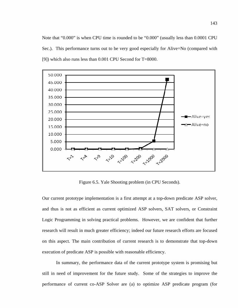
Note that “0.000” is when CPU time is rounded to be “0.000” (usually less than 0.0001 CPU

Sec.). This performance turns out to

[9]) which also runs less than 0.001 CPU Second for T=8000.

Our current prototype implementation is a first attempt at a top

and thus is not as efficient as current optimized ASP solvers, SAT solvers, or Constraint

Logic Programming in solving practical problems. However, we are confiden

research will result in much greater efficiency; indeed our future research efforts are focused

on this aspect. The main contribution of current research is to demonstrate that top

execution of predicate ASP is possible with reasonable

still in need of improvement for the future study. Some of the strategies to improve the

performance of current co

Note that “0.000” is when CPU time is rounded to be “0.000” (usually less than 0.0001 CPU

Sec.). This performance turns out to

[9]) which also runs less than 0.001 CPU Second for T=8000.

Our current prototype implementation is a first attempt at a top

and thus is not as efficient as current optimized ASP solvers, SAT solvers, or Constraint

Logic Programming in solving practical problems. However, we are confiden

research will result in much greater efficiency; indeed our future research efforts are focused

on this aspect. The main contribution of current research is to demonstrate that top

execution of predicate ASP is possible with reasonable

In summary, t

still in need of improvement for the future study. Some of the strategies to improve the

performance of current co

Note that “0.000” is when CPU time is rounded to be “0.000” (usually less than 0.0001 CPU

Sec.). This performance turns out to

[9]) which also runs less than 0.001 CPU Second for T=8000.

Figure

Our current prototype implementation is a first attempt at a top

and thus is not as efficient as current optimized ASP solvers, SAT solvers, or Constraint

Logic Programming in solving practical problems. However, we are confiden

research will result in much greater efficiency; indeed our future research efforts are focused

on this aspect. The main contribution of current research is to demonstrate that top

execution of predicate ASP is possible with reasonable

In summary, the performance data of the current prototype system is promising but

still in need of improvement for the future study. Some of the strategies to improve the

performance of current co

Note that “0.000” is when CPU time is rounded to be “0.000” (usually less than 0.0001 CPU

Sec.). This performance turns out to

[9]) which also runs less than 0.001 CPU Second for T=8000.

Figure 6.5. Yale Shooting problem (in CPU Seconds).

Our current prototype implementation is a first attempt at a top

and thus is not as efficient as current optimized ASP solvers, SAT solvers, or Constraint

Logic Programming in solving practical problems. However, we are confiden

research will result in much greater efficiency; indeed our future research efforts are focused

on this aspect. The main contribution of current research is to demonstrate that top

execution of predicate ASP is possible with reasonable

he performance data of the current prototype system is promising but

still in need of improvement for the future study. Some of the strategies to improve the

performance of current co-ASP Solver are (a) to optimize ASP predicat

Note that “0.000” is when CPU time is rounded to be “0.000” (usually less than 0.0001 CPU

Sec.). This performance turns out to be very good especially for Alive=No (

[9]) which also runs less than 0.001 CPU Second for T=8000.

Yale Shooting problem (in CPU Seconds).

Our current prototype implementation is a first attempt at a top

and thus is not as efficient as current optimized ASP solvers, SAT solvers, or Constraint

Logic Programming in solving practical problems. However, we are confiden

research will result in much greater efficiency; indeed our future research efforts are focused

on this aspect. The main contribution of current research is to demonstrate that top

execution of predicate ASP is possible with reasonable

he performance data of the current prototype system is promising but

still in need of improvement for the future study. Some of the strategies to improve the

ASP Solver are (a) to optimize ASP predicat

Note that “0.000” is when CPU time is rounded to be “0.000” (usually less than 0.0001 CPU

be very good especially for Alive=No (

[9]) which also runs less than 0.001 CPU Second for T=8000.

Yale Shooting problem (in CPU Seconds).

Our current prototype implementation is a first attempt at a top

and thus is not as efficient as current optimized ASP solvers, SAT solvers, or Constraint

Logic Programming in solving practical problems. However, we are confiden

research will result in much greater efficiency; indeed our future research efforts are focused

on this aspect. The main contribution of current research is to demonstrate that top

execution of predicate ASP is possible with reasonable efficiency.

he performance data of the current prototype system is promising but

still in need of improvement for the future study. Some of the strategies to improve the

ASP Solver are (a) to optimize ASP predicat

Note that “0.000” is when CPU time is rounded to be “0.000” (usually less than 0.0001 CPU

be very good especially for Alive=No (

[9]) which also runs less than 0.001 CPU Second for T=8000.

Yale Shooting problem (in CPU Seconds).

Our current prototype implementation is a first attempt at a top-down predicate ASP solver,

and thus is not as efficient as current optimized ASP solvers, SAT solvers, or Constraint

Logic Programming in solving practical problems. However, we are confiden

research will result in much greater efficiency; indeed our future research efforts are focused

on this aspect. The main contribution of current research is to demonstrate that top

efficiency.

he performance data of the current prototype system is promising but

still in need of improvement for the future study. Some of the strategies to improve the

ASP Solver are (a) to optimize ASP predicat

Note that “0.000” is when CPU time is rounded to be “0.000” (usually less than 0.0001 CPU

be very good especially for Alive=No (compared with

Yale Shooting problem (in CPU Seconds).

down predicate ASP solver,

and thus is not as efficient as current optimized ASP solvers, SAT solvers, or Constraint

Logic Programming in solving practical problems. However, we are confident that further

research will result in much greater efficiency; indeed our future research efforts are focused

on this aspect. The main contribution of current research is to demonstrate that top

he performance data of the current prototype system is promising but

still in need of improvement for the future study. Some of the strategies to improve the

ASP Solver are (a) to optimize ASP predicate program (

143

Note that “0.000” is when CPU time is rounded to be “0.000” (usually less than 0.0001 CPU

compared with

down predicate ASP solver,

and thus is not as efficient as current optimized ASP solvers, SAT solvers, or Constraint

t that further

research will result in much greater efficiency; indeed our future research efforts are focused

on this aspect. The main contribution of current research is to demonstrate that top-down

he performance data of the current prototype system is promising but

still in need of improvement for the future study. Some of the strategies to improve the

e program (for

144

example, adding an answer-set template), (b) to take advantage of its underlying Prolog

engine (for example, with constraint, tabling or concurrency), and (c) to use an optimized

look-up table (for example, hash table) whereas current prototype uses a simple list and a

simple list look-up for co-SLDNF positive and negative hypothesis tables.

145

CHAPTER 7

CONCLUSION AND FUTURE WORK

We propose a comprehensive theory of co-LP with co-SLDNF resolution, implemented on

top of YAP Prolog. In doing so, we have proposed a theoretical framework for declarative

semantics of co-SLDNF adapted from Fitting (1985) of Kripke-Kleene semantics with 3-

valued logic) and extended by Fages (1994) for stable model with completion of program.

We have showed the correctness result of co-SLDNF resolution. This provides a concrete

theoretical foundation to handle a cycle of predicates (positive or negative) in ASP. We have

designed and implemented the techniques and algorithms to solve propositional and predicate

ASP programs. We note the limitation of our current approach in inconsistency-checking,

restricted to the class of predicate ASP programs of call-consistent or order-consistent.

Current prototype implementation of co-ASP Solver works for ASP with general

predicates whereas current prototype implementation of ground (propositional) co-ASP

Solver is fully automated and operational. As noted earlier, the performance result of co-

ASP Solver is premature and not competitive, compared with its counterparts. However, we

believe that the perspective and future of co-ASP Solver is very promising. Some of the

advantages and competitive edge achieved by co-ASP Solver are noteworthy. First (1), it

solves predicate ASP program without grounding. If grounding becomes a bottleneck,

current ASP Solvers become helpless. Second (2), it extends ASP language into first order

logic with function symbols and infinite ground (rational) atoms. Its expressive power is

now extended one level up to handle an infinite objects and streams for modeling and

146

verification. Third (3), co-ASP Solver presents an alternative paradigm and ASP-strategy

radically different from current ASP Solvers, to provide a possibility toward the development

of a hybrid ASP Solver, combining the best of these two paradigms (bottom-up and top-

down). Fourth (4), co-ASP Solver provides a rich alternative semantics of partial or total

model and of gfp or lfp. Finally (5), current implementation is built on top of Prolog

environment that co-ASP Solver can utilize and take advantage of all of the existing Prolog

language features, built-in functions and its extensions including tabling and constraint logic

programming. Thus co-ASP Solver is very powerful, not only to solve current ASP

programs but also to extend its power and usability to Predicate ASP programs, on top of

Prolog system and its capability.

Our future works for co-LP include: (1) a language specification of co-LP with

coinductive built-in predicates and system libraries, (2) its optimization and tuning, (3) its

extension to concurrent and parallel processing, and (4) exploring co-LP to new domains of

applications including modeling checking and verification. Another challenging future work

is to extend the rational restriction of co-LP into the irrational domain, possibly using

symbolic formula to represent an irrational terms and atoms and its derivation with delayed

evaluation with limitation of the length (that is, approximation with tolerance or error range).

Our future works for co-ASP Solver include: (1) a fully automated and optimized co-

ASP Solver, (2) a utility to transform a ASP program into a co-ASP program, (3) a utility to

check inconsistency of ASP program extending current restriction, and (4) extending a range

of ASP applications with performance monitoring and benchmarking.

Further, we showed how co-SLDNF resolution can be used to elegantly develop

Boolean SAT solvers. The SAT solvers thus obtained are simpler and more elegant than

147

solvers realized via ASP. Our future work is directed towards making the implementation of

both co-ASP and co-SAT more efficient so as to be competitive with the state-of-the-art

solvers for ASP and SAT. Another significant result is the application of co-LP to the

analysis of rational sequences and model checking. We have showed how co-LP can be

applied to the analysis of rational sequence and state-transition system, and model checking.

We have implemented a naïve co-LTL solver and co-CTL solver, with the correctness

results. Our future work is directed towards making the implementation of both co-LTL and

co-CTL more efficient to be competitive with the state-of-the-art LTL and CTL solvers.

The performance data of the current prototype system is promising but still in need of

improvement if we compare it with performance on other existing solvers (even after taking

the cost of grounding the program into account). Our main strategy for improving the

performance of our current co-ASP solver is to interleave the execution of candidate answer

set generation and “nmr_check”. This generation and testing has to be interleaved in the

manner of constraint logic programming to reduce the search space. Additional

improvements can also be made by improving the representation and look-up of positive and

negative hypothesis tables during co-SLDNF (for example, by using a hash table, or a trie

data-structure).

148

REFERENCES

Aczel, Peter. 1977. An introduction to inductive definitions. In K. Jon Barwise, editor,

Handbook of Mathematical Logic, pages 739–782. North-Holland, Amsterdam. ———. 1988. Non-well-founded Sets, volume 14 of CSLI Lecture Notes. CSLI Publications,

Stanford, CA. Aiello, L. C., and F. Massacci. 2001. Verifying Security Protocols as Planning in Logic

Programming. ACM Transactions on Computational Logic 2(4), pp. 542–580. Aït-Kaci, Hassan. 1991. Warren’s abstract machine: A tutorial reconstruction. MIT Press. Antoniou, Grigoris. 1997. Nonmonotonic reasoning. MIT Press. Apt, Krzysztof. 1990. Logic programming. Handbook of Theoretical Computer Science,

493–574. MIT Press. ———. 2003. Principles of Constraint Programming. Cambridge University Press. Apt, Krzysztof, Howard Blair, and Adrian Walker. 1988. Towards a theory of declarative

knowledge. In Jack Minker, editor, Foundations of Deductive Databases and Logic Programming, pages 89-148. Morgan Kaufmann, San Mateo, CA, 1988.

Apt, Krzysztof, and Ronald Bol. 1994. Logic programming and negation: a survey. Journal

of Logic Programming, 19,20:9–71. Apt, Krzysztof, and M. H. van Emden. 1982. Contributions to the theory of logic

programming. Journal of ACM, 29(3):841–862. Apt, Krzysztof, and Mark Wallace. 2007. Constraint logic programming using Eclipse.

Cambridge University Press. Arbib, Bijan, and Daniel M. Berry. 1987. Operational and denotational semantics of

PROLOG. Journal of Logic Programming, 4:309–329. Aura, T., Bishop, M., Sniegowski, D. 2000. Analyzing Single-Server Network Inhibition. In,

Proceedings of the IEEE Computer Security Foundations Workshop, 108-117. Babovich, Y., Esra Erdem, and Vladimir Lifschitz. 2000. Fages’ theorem and answer set

programming. In Proc. NMR-2000.

149

Baader, F., and W. Snyder. 2001. Unification theory. In A. Robinson and A. Voronkov, editors, Handbook of Automated Reasoning, volume I, chapter 8, pages 445–532. Elsevier Science.

Baader, F., D. Calvanese, D. L. McGuinness, D. Nardi, and P. F. Patel-Schneider. 2003. The

Description Logic Handbook: Theory, Implementation, Applications. Cambridge University Press, Cambridge, UK.

Baier, C., and J. Katoen. 2008. Principles of Model Checking. MIT Press. Bansal, Ajay. 2007. Next Generation Logic Programming Systems. Ph.D. Dissertation. The

University of Texas at Dallas. Baral, Chitta. 2003. Knowledge Representation, Reasoning and Declarative Problem

Solving. Cambridge University Press. Baral, Chitta, and Michael Gelfond. 1994. Logic programming and knowledge

representation. Journal of Logic Programming,19,20:73–148. Barwise, Jon, and Lawrence Moss. 1996. Vicious Circles: On the Mathematics of Non-

Wellfounded Phenomena. CSLI Publications, Stanford, California, 1996. Baselice, S., P. Bonatti, and M. Gelfond. 2005. Towards an Integration of Answer Set and

Constraint Solving. In: ICLP'05, 52–66. Springer. Babovich. Y. 2002. CModels. http://www.cs.utexas.edu/users/tag/cmodels. html. Babovich. Yuliya, and Vladimir Lifschitz. 2003. Computing Answer Sets using program

completion. unpublished draft. www.cs.utexas.edu/users/tag/cmodels/cmodels-1.ps Babovich. Yuliya, Esra Erdem, and Vladimir Lifschitz. 2000. Fages’ theorem and answer set

programming. In Proc. NMR-2000. Belnap, Jr., N. D. 1977. A Useful four-valued logic, In J. Michael Dunn and G. Epstein

(editors), Modern Uses of Multiple-Valued Logic, 8–37. Bibel, W. 1982. Automated Theorem Proving. Vieweg, Braunschweig. Bird, R. 1976. Programs and Machines. Wiley, New York. Bonatti, P., E. Pontelli, and T. C. Son. 2008. Credulous Resolution for Answer Set

Programming. In, AAAI'08. Bratko, Ivan. 2001. PROLOG: Programming for artificial intelligence. 3rd ed. Addison-

Wesley.

150

Brewka, Gerhard. 1991. Nonmonotonic reasoning: Logical foundations of commonsense. Cambridge University Press.

Brewka, Gerhard, Jürgen Dix, and Kurt Konolige. 1997. Nonmonotonic reasoning: An

overview. CSLI Lecture Notes Number 73, CSLI Publications. Stanford, CA. Cavedon, L, and J. W. Lloyd. 1989. A completeness theorem for SLDNF-resolution. In

Journal of Logic Programming, 7(3), pages 177–192. Chan, David. 1988. Constructive negation based on the completed database. In R. Kowalski

and K. Bowen (editors), Proc. of 5th JICSLP, pages 111-125. Chan, David, and Mark Wallace. 1989. A Treatment of Negation during partial evaluation. In

Meta-programming in logic programming, pages 299-317. MIT Press. Chang, Chin-Liang, and Richard Char-Tung Lee. 1973. Symbolic logic and mechanical

theorem proving. Academic Press. New York. Chen, Weidong, Terrance Swift, and David Warren. 1993. Goal-directed evaluation of well-

founded semantics for XSB. In Dale Miller, editor, Proc. ILPS-93, page 679. Chen, Weidong, Terrance Swift, and David Warren. 1995. Efficient top-down computation

of queries under the well-founded semantics. In Journal of Logic Programming, volume 24(3), pages 161–199.

Chen, Weidong, and David Warren. 1996. Tabled Evaluation with Delaying for General

Logic Programs. In Journal of the ACM, volume 43(1), pages 20–74. Springer Verlag.

Clark, K. L. 1978. Negation as Failure. In: Gallaire, H., Minker, J. (eds.) Logic and Data

Bases. 293–322. Plenum Press, New York. Clarke, Edmund M., Orna Grumberg, and Doron A. Peled. Model Checking. The MIT Press,

Cambridge, Massachusetts, 1999. Clocksin, W. F., and C. S. Mellish. 2003. Programming in Prolog: Using the ISO standard.

5th edition. Springer. Colmerauer, Alain. 1978. Prolog and Infinite Trees. In: Clark, K.L., Tarnlund, S.-A. (eds.)

Logic Programming. pp. 293–322. Prenum Press, New York. ———. 1984. Equations and inequations on finite and infinite trees. In FCCS-84

Proceedings International Conference on Fifth Generation Computer Systems, pages 85–99, Tokyo, ICOT.

———. 1990. An introduction to Prolog III. Communications of the ACM, 33(7):69–90.

151

Colmerauer, Alain, and P. Roussel. 1996. The birth of PROLOG. In History of Programming Languages. ACM Press/Addison-Wesley.

Cortesi, A., and G. Filé. 1990. Graph properties for normal logic programs. In Proc. 5th

Conv. Nat. sulla Programmzione Logica GULP’90, Padova. Costa, V. S., an d R. Yang. 1991. Andorra-I: a Parallel Prolog system that transparently

exploits both And- and Or-Parallelism. In (PPoPP), pages 83–93. Costa, Vítor Santos, David H. D. Warren, and Rong Yang. 1991. Andorra I: a parallel Prolog

system that transparently exploits both And-and or-parallelism, ACM SIGPLAN Notices, v.26 n.7, p.83-93.

Courcelle, B. 1983. Fundamental properties of infinite trees. Theoretical Computer Science

25(2):95–169. Davey, B. A., and H. A. Priestley. 2002. Introduction to lattices and order. 2nd ed.

Cambridge University Press. Davis, M. and H. Putnam. 1960. A computing procedure for quantification theory. Journal of

the Association for Computing Machinery, 7:201–215. Dimopoulos, Y., B. Nebel, and J. Koehler. 1997. Encoding Planning Problems in

Nonmonotonic Logic Programs. In: Proceedings of the Fourth European Conference on Planning, 169–181. Springer-Verlag.

Dix, Jürgen, Ulrich Furbach, and Ilkka Niemelä. 2001. Nonmonotonic reasoning: Towards

efficient calculi and implementations. In Andrei Voronkov and Alan Robinson, editors, Handbook of Automated Reasoning. Elsevier-Science-Press.

Dix, Jürgen. 1995a. Semantics of logic programs: Their intuitions and formal properties. An

overview. In Andre Fuhrmann and Hans Rott, editors, Logic, Action and Information – Essays on Logic in Philosophy and Artificial Intelligence, pages 241–327. DeGruyter.

———. 1995b. A Classification Theory of Semantics of Normal Logic Programs: ii. Weak

Properties. Fundamenta Informaticae 22(3), 257–288. Docets, Kees. 1993. Levantionis Laus. In: Journal of Logic Programming 3(5):487–516. ———. 1994. From logic to logic programming. MIT Press. Dovier, A., A. Formisano, and E. Pontelli. 2005. A Comparison of Clp(Fd) and Asp

Solutions to Np-Complete Problems. In: ICLP'05, 67–82. Springer. Doyle, J. 1979. A truth maintenance system. Artificial Intelligence, vol. 12, 231–272.

152

Dung, P. M., and K. Kanchanasut. 1989. A fixpoint approach to declarative semantics of logic programs. In NACLP’89. MIT Press.

———. 1989. On the generalized predicate completion of non-Horn program. In Logic

Programming: Proc. of the North American Conference. MIT Press. pages 587-603. East, D., and M. Truszczyński. 2001. More on Wire Routing with Asp. In, AAAI Spring

2001 Symposium, 39–44. Eiter, Thomas, Nicola Leone, Christinel Mateis, Gerald Pfeifer, and Francesco Scarcello.

1997. A deductive system for non-monotonic reasoning. In Proceedings of the 4th International Conference on Logic Programming and Nonmonotonic Reasoning, pages 363–374. Springer-Verlag.

———. 1998. The KR system DLV: Progress report, comparisons and benchmarks. In

Anthony Cohn, Lenhart Schubert, and Stuart Shapiro, editors, Proc. Sixth Int’l Conf. on Principles of Knowledge Representation and Reasoning, pages 406–417.

Eiter, Thomas, Wolfgang Faber, Nicola Leone, and Gerald Pfeifer. 1999. The diagnosis

frontend of the DLV system. The European Journal on Artificial Intelligence, 12(1–2):99–111.

Emden, Maarten, van Emden, and Robert Kowalski. 1976. The semantics of predicate logic

as a programming language. Journal of the ACM, 23(4):733–742. Enderton, Herbert. 2001. A mathematical introduction to logic. 2nd ed. Academic Press. Erdem, Esra, and Vladimir Lifschitz. 1999. Transformations of logic programs related to

causality and planning. In Logic Programming and Non-monotonic Reasoning: Proc. Fifth Int’l Cotif. (Lecture Notes in Artificial Intelligence 1730), pages 107–116.

———. 2001. Fages’ theorem for programs with nested expressions. In ICLP’01, 242–254. Erdem, Esra, Vladimir Lifschitz, and Martin Wong. 2000. Wire Routing and Satisfiability

Planning. In: Proceedings of the First International Conference on Computational Logic, Automated Deduction: Putting Theory into Practice, 822–836. Springer-Verlag.

Erdem, Esra, and Vladimir Lifschitz. 2001a. Fages’ theorem for programs with nested

expressions. In Proceedings of the Seventeenth International Conference on Logic Programming, pages 242–254.

———. 2001b. Transitive closure, answer sets, and predicate completion. In Working Notes

of the AAAI Spring Symposium on Answer Set Programming.

153

———. 2002. Tight logic programs. To appear in the Special Issue of the Theory and Practice of Logic Programming Journal on Answer Set Programming.

Erdem, Esra, Vladimir Lifschitz, and Martin Wong. 2000. Wire routing and satisfiability

planning. In Proc. CL-2000, pages 822–836. Erdem, Esra, Vladimir Lifschitz, Luay Nakhleh, and Donald Ringe. 2002. Reconstructing the

evolutionary tree of natural languages using answer set programming. Submitted for publication.

Esparza, J., and K. Heljanko. 2001. Implementing Ltl Model Checking with Net Unfoldings.

In: Proceedings of the 8th International SPIN Workshop on Model Checking of Software (SPIN'01), 37–56. Springer-Verlag.

Fages, François. 1990. A new fixpoint semantics for general logic programs compared with

the well-founded and the stable model semantics. Journal of New Gen. Computing, pages 442–458, 1994.

———. 1994. Consistency of Clark’s completion and existence of stable models. Journal of

Methods of Logic in Computer Science, 1:51–60, 1994. Falaschi, M., G. Levi, and C. Palamidessi. 1983. The Formal Semantics of Processes and

Streams in Logic Programming. Colloquia Mathematica Societatis János Bolyai 42, 363–377.

Falaschi, M., G. Levi, C. Palamidessi, and M. Martelli. 1989. Declarative Modeling of the

Operational Behavior of Logic Languages. Theoretical Computer Science 69:289–318.

Falaschi, M., G. Levi, M. Martelli, and C. Palamidessi. 1993. A model-theoretic

reconstruction of the operational semantics of logic programs. Information and Computation 103:86–113.

Ferraris, P., and V. Lifschitz. 2005. Mathematical Foundations of Answer Set Programming.

In: We Will Show Them! Essays in Honour of Dov Gabbay. 615–664. King’s College Publications.

———. 2007. A New Perspective on Stable Models. In: IJCAI'07, 372–379. Fikes, Richard, and Nils Nilsson. 1971. STRIPS: A new approach to the application of

theorem proving to problem solving. Artificial Intelligence, 2(3–4):189–208. Fitting, M. C. 1983. Notes on the Mathematical Aspects of Kripke’s Theory of Truth. Notre

Dame Journal of Formal Logic 27(1): 75–88.

154

———. 1985. A Kripke/Kleene Semantics for Logic Programs. Journal of Logic Programming 2, 295–312.

———. 1988. Logic rogramming on a topological bilattice. Fundamenta Informaticae. 209–

218. ———. 1989a. Negation as refutation. Proceedings Fourth Annual Symposium on Logic in

Comptuer Science, 63–70. IEEE Computer Society Press. ———. 1989b. Billatice and the theory of truth. Journal of Philosophical Logic, vol. 18.

225–256. ———. 1991. Bilattice and the semantics of logic programming. Journal of Logic

Programming 11. 91–106. ———. 1993. The Family of Stable Models. Journal of Logic Programming 17. 197–225. Fitting, M. C., and R. L. Mendelsohn. 1998. First-order modal logic. Synthese Library vol.

277. Kluwer Academic publishers. Gebser, M., and T. Schaub. 2006. Tableau Calculi for Answer Set Programming. In Interna-

tional Conference on Logic Programming (ICLP), pages 11–25. Springer. Gelfond, Michael. 1987. On stratified autoepistemic theories. In Proc. AAAI-87, pages 207–

211, 1987. Gelfond, Michael, and Joel Galloway. 2001. Diagnosing dynamic systems in AProlog. In

Working Notes of the AAAI Spring Symposium on Answer Set Programming. Gelfond, Michael, and Vladimir Lifschitz. 1988. The stable model semantics for logic

programming. In Robert Kowaiski and Kenneth Bowen, editors, Logic Programming: Proc. Fifth Int’l Conf. and Symp., pages 1070–1080.

———. 1990. Logic programs with classical negation. In David Warren and Peter Szeredi,

editors, Logic Programming: Proc. Seventh Int’l Conf., pages 579–597. ———. 1991. Classical negation in logic programs and disjunctive databases. New

Generation Computing, 9:365–385. ———. 1998. Action languages. Electronic Transactions on Al, 3:195–210. Gelfond, Michael, Vladimir Lifschitz, Halina Przymusiñska, and Miroslaw Truszczyñski.

1991. Disjunctive defaults. In James Allen, Richard Fikes, and Erik Sandewall, editors, Principles of Knowledge Representation and Reasoning: Proc. Second Int’l Conf., pages 230–237, 1991.

155

Goldin, D., and D. Keil. 2001. Interaction, Evolution and Intelligence. In, Proc. Congress on Evolutionary Computing.

Golson, W. 1988. Toward a Declarative Semantics for Infinite Objects in Logic

Programming. Journal of Logic Programming 5:151–164. Gordon, A. 1995. A Tutorial on Co-induction and Functional Programming. In Workshops in

Computing (Functional Programming), pages 78–95. Springer, 1995. Gupta, G., A. Bansal, R. Min, L. Simon, and A. Mallya. 2007. Coinductive Logic

Programming and Its Applications. (Tutorial Paper). In: Proc. of ICLP07, 27–44. Gupta, Gopal, and Enrico Pontelli. 1997. A constraint-based approach for specification and

verification of real-time systems. In IEEE Real-Time Systems Symposium, 230–239. Hein, J. 1992. Completions of Perpetual Logic Programs. Theoretical Computer Science 99:

65–78. Heljanko, K. 1999. Using Logic Programs with Stable Model Semantics to Solve Dead-Lock

and Reachability Problems for 1-Safe Petri Nets. Fundamenta Informaticae 37(3), pages 247–268.

Heljanko, K., and I. Niemelä. 2003. Bounded Ltl Model Checking with Stable Models.

Theory and Practice of Logic Programming 3(4&5):519–550. Horn, Alfred. 1951. 1951. On sentences which are true of direct unions of algebras. Journal

of Symbolic Logic 16:14-21. Hoare, C. A. R. 1969. An axiomatic basis for computer programming. Communications of

the ACM 12(10):576-580.

Huth, M., and M. Ryan. 2004. Logic in Computer Science: Modeling and Reasoning About

Systems. Cambridge University Press. Jacobs, B., and J. Rutten. 1997. A Tutorial on (Co)Algebras and (Co)Induction. EATCS

Bulletin 62, 222–259. Jaffar, Joxan, Jean-Louis Lassez, and John Lloyd. 1983. Completeness of the negation as

failure rule. In Proc. IJ CAI’83, pages 500–506. Jaffar, Joxan, Jean-Louis Lassez, and M. J. Maher. 1984. A theory of complete logic

programs with equality. In Proc. Conference on Fifth Generation Computer Systems, Tokyo, 175-184.

———. 1986a. Some issues and trends in the semantics of logic programming. In ICLP’86,

pages 223–241.

156

———. 1986b. A logic programming language Scheme. In Logic programming: Relations, Functions and Equations. D. DeGroot and G. Lindstrom (Eds), Prentice-Hall, 441-467.

———. 1986c. Prolog-II as an instance of the logic programming language scheme. In:

Formal Descriptions of Programming Concepts III. M. Wirsing (ed.), North-Halled, 275-299.

Jaffar, Joxan, A. Santosa, and R. Voicu. 2005. Modeling Systems in Clp with Coinductive

Tabling. ICLP'05, 412–413. ———. 2008. A Coinduction Rule for Entailment of Recursively Defined Properties. CP'08. Jaffar, Jaxon, and Peter J. Stuckey. 1986. Semantics of infinite tree logic programming.

Theoretical Computer Science, 46(2-3):141–158. Janhunen, T., I. Niemelä, D. Seipel, P. Simons, and J.-H. You. 2006. Unfolding Partiality and

Disjunctions in Stable Model Semantics. ACM Transactions on Computational Logic 7(2), 1–37.

Jaume, M. 1998. Logic programming and co-inductive definitions. In P. Clote and H.

Schwichtenberg (Eds.): Computer Science Logic Conference (CSL2000), LNCS 1862, pages 343-355. Springer-Verlag, Berlin.

———. 2002. On Greatest Fixpoint Semantics of Logic Programming. Journal of Logic and

Computation 12(2):321-342. Jacobs, B. 2005. Introduction to Coalgebra: Towards Mathematics of States and Observation.

Draft Manuscript. http://www.cs.ru.nl/B.Jacobs/CLG/JacobsCoalgebraIntro.pdf Kautz, H., and Bart Selman. 1992. Planning as Satisfiability. In Proceedings of European

Conference on Artificial Intelligence (ECAI-92), 359–363. ———. 1996. Pushing the envelope: planning, propositional logic and stochastic search. In

Proc. AAAI-96, pages 1194–1201. Kautz, Henry, David McAllester, and Bart Selman. 1996. Encoding plans in propositional

logic. In Principles of Knowledge Representation and Reasoning: Proc. of the Fifth Int’l Conf., pages 374–384.

Kleene, S. C. 1950. Introduction to Methmathematics. Van Nostrand. ———. 1967. Mathematical Logic. John Wiley. Knight, Kevin. 1989. Unification: a multidisciplinary survey. ACM computing surveys,

March 1989, 21(1):93–124.

157

Kowaiski, Robert A. 1974. Predicate logic as programming language. In Jack L. Rosenfeld, editor, Proceedings of International Federation of Information Processing Conference, pages 569–574, Stockholm, Sweden. North–Holland.

———. 1979. Algorithm = Logic + Control. Communications of ACM 27(7):424–436. Kowaiski, Robert A., and Donald Kuehner. 1971. Linear resolution with selection function.

Journal of Artificial Intelligence,2:22–260. Kripke, Saul. 1975. Outline of a Theory of Truth. Journal of Philosophy 72, pages 690–716. Kunen, K. 1987. Negation in logic Programming. Journal of Logic Programming, 4(4):289–

308. ———. 1989. Signed data dependencies in logic programs. Journal of Logic Programming,

7(3):231–245. Lassez, J.-L., and M. J. Maher. 1984. Closure and fairness in semantics of programming

logic. In Theoretical Computer Science 29:164–184. ———. 1985. Optimal fixedpoints of logic programs. In Theoretical Computer Science

39:15–25. Lassez, J.-L., V. L. Nguyen, and M. J. Maher. 1982. Fixed point theorems and semantics; a

folk tale. In Information Processing Letters 14(3):112–116. Levi, Giorgio, and Catuscia Palamidessi. 1988. Contributions to the semantics of logic

perpetual processes. Acta Informatica 25, 691-711. Lifschitz, Vladimir. 1988. On the declarative semantics of logic programs with negation. In

Jack Minker, editor, Foundations of Deductive Databases and Logic Programming, pages 177–192. Morgan Kaufmann, San Mateo, CA.

———. 1996a. Foundations of logic programming. In Brewka, G. (ed.), Principles of

Knowledge Representation. CLSI Publications. 69-128. ———. 1996b. Two components of an action language. In Working Papers of the Third

Symposium on Logical Formalizations of Cornmonsense Reasoning. ———. 1999a. Action Languages, Answer Sets and Planning. In: The Logic Programming

Paradigm: A 25-Year Perspective. pages 357–373. Springer-Verlag. ———. 1999b. Answer set planning. In Proc. ICLP-99, pages 23–37. ———. 2000. Missionaries and cannibals in the causal calculator. In Principles of

Knowledge Representation and Reasoning:Proc. Seventh Int’l Conf., pages 85–96.

158

———. 2002. Answer set programming and plan generation. Artificial Intelligence 138:39–54.

Lifschitz, Vladimir, and Hudson Thrner. 1994. Splitting a logic program. In Pascal Van

Hentenryck, editor, Proc. Eleventh Int’l Conf. on Logic Programming, pages 23–37. ———. 1999. Representing transition systems by logic programs. In Logic Programming

and Non-monotonic Reasoning: Proc. Fifth Int’l Conf. (Lecture Notes in Artificial Intelligence 1730), pages 92–106.

Lifschitz, Vladimir, and Thomas Woo. 1992. Answer sets in general nonmonotonic

reasoning (preliminary report). In Bernhard Nebel, Charles Rich, and William Swartout, editors, Proc. Third Int’l Conf. on Principles of Knowledge Representation and Reasoning, pages 603–614.

Lifschitz, Vladimir, Lappoon R. Tang, and Hudson Thrner. 1999. Nested expressions in logic

programs. Annals of Mathematics and Artificial Intelligence, 25:369–389. Lifschitz, Vladimir, David Pearce, and Agustin Valverde. 2001. Strongly equivalent logic

programs. ACM Transactions on Computational Logic. Lin, F., and Y. Zhao. 2002. ASSAT: Computing Answer Sets of Logic Programs by SAT

Solvers. In AAAI/IAAA, pages 112–117. AAAI/MIT Press. ———. 2004. Assat: Computing Answer Sets of a Logic Program by Sat Solvers. Artificial

Intellegence 157(1-2), pp. 115–137. Lloyd, J. W. 1987. Foundations of Logic Programming. 2nd Edition. Springer. Lloyd, J. W., and Rodney Topor. 1984. Making Prolog more expressive. Journal of Logic

Programming, 3:225–240. Lloyd, J. W., and J. C. Shepherdson. 1991. Partial evaluation in logic programming. Journal

of Logic Programming 4, 289–308. Loveland, D. W. 1970. A linear format for resolution. In Proceedings of the IRIA Symposium

on Automatic Demonstration, pages 147-162, New York, 1970. Springer-Verlag. ———. 1978. Automated Theorem Proving: A Logical Basis. North Holland, New York. Maher, M. J. 1988a. Complete Axiomatizations of the Algebras of Finite, Rational and

Infinite Trees. In: Proc. 3rd Logic in Computer Science Conference, 348–357. Edinburgh, UK.

159

———. 1988b. Complete Axiomatizations of Finite, Rational and Infinite Trees. IBM Research Report, Thomas J. Watson Research Center, Yorktown Height, NY. available: http://www.cse.unsw.edu.au/~mmaher/pubs/trees/axiomatizations.pdf

Manna, Zohar and Adi Shamir. 1972. Fixpoint Approach to the Theory of Computation. In

Communications of the ACM. 15(7):528–536. ———. 1976a. The optimal fixedpoint of recursive programs, In Proc. Symp. on Theory of

Computing, Albuquerque, N.M.. ———. 1976b. A new approach to recursive programs, In Jones, A. K. (editor), Perspectives

on Computer Science, Academic Press, New York. 103–124. ———. 1976c. The theoretical aspects of the optimal fixedpoint. In SIAM J. Computing

5(3):414–426. ———. 1977. The optimal approach to recursive programs. In Communications of the ACM.

20(11):824–831. Marek, W., and V. S. Subrahmanian. 1989. The relationship between logi program semantics

and non-monotonic reasoning. In Proc. Sixth International Conference on Logic Programming.

Marek, W., and M. Truszczyński. 1999. Stable Models and an Alternative Logic

Programming Paradigm. In The Logic Programming Paradigm: a 25-Year Perspective (NACLP’89). pages 375-398. Springer-Verlag.

Marriott, Kim, and Peter Stuckey. 1998. Programming with Constraints: An Introduction.

The MIT Press, Cambridge, Massachusetts. Martelli, Alberto, and Ugo Montanari. 1982. An efficient unification algorithm. ACM

Transactions on Programming Languages and Systems, 4(2):258 McCarthy, John. 1959. Programs with common sense. In Proc. Teddington Conf. on the

Mechanization of Thought Processes, pages 75–91, London. Her Majesty’s Stationery Office.

———. 1980. Circumscription - A form of non-monotonic reasoning. Artificial Intelligence,

13:27–39. ———. 1986. Applications of circumscription to formalizing common sense knowledge.

Artificial Intelligence, 26(3):89–116. Milne, R. and C. A. Starchey. 1976. Theory of programming language and semantics.

Chapman and Hall, London.

160

Milner, Robin. 1980. A Calculus of Communicating Systems, volume 92 of Lecture Notes in Computer Science. Springer-Verlag, Berlin.

———. 1989. A Communication and Concurrency. Prentice Hall. ———. 1999. Communicating and Mobile Systems: the Pi-Calculus. Cambridge University

Press. Milner, Robin, and Mads Tofte. 1991. Co-induction in relational semantics. Theoretical

Computer Science 87(1):209–220. Min, Richard, Ajay Bansal, and Gopal Gupta. 2009. Towards Predicate Answer Set

Programming via Coinductive Logic Programming. AIAI’09. Min, Richard and Gopal Gupta. 2008a. Negation in Coinductive Logic Programming.

Technical Report UTDCS-34-08. Computer Science Department. The University of Texas at Dallas. http://www.utdallas.edu/~rkm010300/research/co-SLDNF.pdf

———. 2008b. Predicate Answer Set Programming with Coinduction. Technical Report

(Draft). Computer Science Department. The University of Texas at Dallas. http://www.utdallas.edu/~rkm010300/research/co-ASP.pdf

———. 2009. Coinductive Logic Programming and its Application to Boolean SAT. Flairs

2009. Moore, Robert. 1985. Semantical considerations on nonmonotonic logic. Artificial

Intelligence, 25(1):75–94. Muggleton, Stephen. 1992. Inductive Logic Programming. Academic Press, New York. Mycroft, Alan. 1984. Logic programs and many-valued logic. In Proceedings of the

Symposium of Theoretical Aspects of Computer Science 166:274-286. Nait Abdallah, M. A. 1984. On the interpretation of infinite computations in logic

programming. In ICALP’84, pages 358–370, Antwerp, Belgium, Springer-Verlag. Nerode, Anil, and Richard A. Shore. 1997. Logic for applications. 2nd ed. Springer. Niemelä, Ilkka. 1999. Logic Programs with Stable Model Semantics as a Constraint

Programming Paradigm. Annals of Mathematics and Artificial Intelligence 25(3-4), pp. 241–273.

———. 2003. Answer Set Programming: From Model Computation to Problem Solving. In,

Proceedings of CADE-19 Workshop on Model Computation - Principles, Algorithms, Applications.

161

Niemelä, Ilkka, and Patrik Simons. 1996a. Efficient Implementation of the Well-Founded and Stable Model Semantics. In: Maher, M. (ed.) Proceedings of the Joint International Conference and Symposium on Logic Programming, pp. 289–303. The MIT Press.

———. 1996b. Efficient Implementation of the Well-Founded and Stable Model Semantics.

Fachbericht Informatik 7–96. www.uni-koblenz.de/fb4/publikationen/gelbereihe/ ———. 1997. Smodels – an Implementation of the Stable Model and Well-Founded

Semantics for Normal Logic Programs. In: Proceedings of the 4th International Conference on Logic Programming and Non-Monotonic Reasoning, pp. 420–429. Springer-Verlag.

Nilsson, Ulf, and Jan Maluszynski. 1995. Logic, Programming and Prolog. (2nd ed.). John

Wiley & Sons Ltd. Nogueira, M., M. Balduccini, M. Gelfond, R. Watson, and M. Barry. 2001. An a-Prolog

Decision Support System for the Space Shuttle. In: PADL'01, pp. 169–183. Springer-Verlag.

Park, David. 1981. Concurrency and automata on infinite sequences. In Theoretical

Computer Science 104:167–183. Pereira, L. M., and A. M. Pinto. 2005. Revised Stable Models - a Semantics for Logic

Programs. In: Procs. 12th Portuguese Intl.Conf. on Artificial Intelligence (EPIA'05), pp. 29–42. Springer.

Pfeifer, G., N. Leone, and W. Faber. DLV. http: //www.dbai.tuwien.ac.at/proj/dlv Pierce, Benjamin C. 2002. Types and Programming Languages. The MIT Press, Cambridge,

Massachusetts. Pierro, A. Di. 1994. Negation andn infinite computations in logic programming. Ph.D.

Thesis. Università di Pisa-Genova-Udine. Przymusinski, Teodor. 1998. On the declarative semantics of deductive databases and logic

programs. In Jack Minker, editor, Foundations of Deductive Databases and Logic Programming, pages 193–2 16. Morgan Kaufmann, San Mateo, CA, 1988.

Ramakrishna, Y. S., C. R. Ramakrishnan, I. V. Ramakrishnan, Scott A. Smolka, Terrance

Swift, and David Scott Warren. 1997. Efficient model checking using tabled resolution. In CAV, pages 143–154.

Reiter, Raymond. 1978. On Closed World Data Bases. In Jack Minker (editor), Foundations

of Deductive Databases and Logic Programming, pages 55–76. Morgan Kaufmann, San Mateo, CA.

162

———. 1980. A logic for default reasoning. Artificial Intelligence, 13:81–132. ———. 2001. Knowledge in Action: Logical Foundations for Specifying and Implementing

Dynamical Systems. The MIT Press. Robinson, J. A.. 1965. A machine-oriented logic based on the resolution principle. Journal of

the ACM. 12:23–41. ———. 1971. Computational logic: The unification computation. In B. Meltzer and D.

Michie, editors, Machine Intelligence 6, pages 63–72. Edinburgh University Press, Edinburgh.

Roussel, Philippe. 1975. PROLOG, manuel de reference at d’utilisation. Technical report,

Université d’Aix-Marseille II. Sangiorgi, Davide and David Walker. 2001. The π-Calculus: a Theory of Mobile Processes.

Cambridge University Press. Sato, T. 1990. Completed Logic Programs and Their Consistency. Journal of Logic

Programming 9(1), pages 33–44. Schlechta, Karl. 1991. Nonmonotonic logics: Basic concepts, results, and techniques. LNCS

1187, Springer. Schlif, J. S. 1990. The expressive powers of the logic programming semantics with negation,

PODS’90, pages 205-217. Schmidt, David A. 1994. The Structure of Typed Programming Languages. MIT Press. Schuppan, Viktor, and Armin Biere. 2006. Liveness checking as safety checking for infinite

state spaces. Electr. Notes Theor. Comput. Sci, 149(1):79–96. Scott, Michael L. 2006. Programming Language Pragmatics. 2nd edition. Morgan

Kaufmann. Shen, Y.-D., J.-H. You, and L.-Y. Yuan. 2004. Enhancing Global Sls-Resolution with Loop

Cutting and Tabling Mechanisms. Theoretical Computer Science 328(3):271–287. Shepherdson, John C. 1984. Negation as failure: A comparison of Clark’s completed data

base and Reiter’s closed world assumption. Journal of Logic Programming 1(1):51–79.

———. 1985. Negation as failure II. Journal of Logic Programming 2(3):185–202.

163

———. 1988. Negation in logic programming. In Jack Minker, editor, Foundations of Deductive Databases and Logic Programming, pages 19–88. Morgan Kaufmann, San Mateo, CA.

SICS. 2002. SICStus User Manual. Version 3.10.0. Swedish Institute of Computer Science. Simon, Luke. 2006. Extending Logic Programming with Coinduction. Ph.D. Dissertation.

The University of Texas at Dallas, Richardson, Texas. Simon, Luke, Ajay Bansal, Ajay Mallya, and Gopal Gupta. 2007. Co-Logic Programming.

In: Proc. ICALP'07, pp. 472–483. Springer. ———. 2006. Coinductive Logic Programming. In: ICLP'06. LNCS 4079, pp. 330–344.

Springer. Simons, Patrik. 1997. Towards constraint satisfaction through logic programs and the stable

model semantics. Technical Report 47, Helsinki University of Technology. ———. 1999. Extending the stable model semantics with more expressive rules. In Logic

Programming and Non-rnonotonic Reasoning: Proc. Fifth Int’l Conf. (Lecture Notes in Artificial Intelligence 1730), pages 305–316.

———. 2000. Extending and implementing the stable model semantics. Technical Report

58, Helsinki University of Technology. Simons, Patrik, Ilkka Niemelä, and Timo Soininen. 2002. Extending and implementing the

stable model semantics. Artificial Intelligence, 138(1-2):181–234. Simons, Patrik, T. Syrjanen. 2003. Smodels (Version 2.27) and Lparse (Version 1.0.13) - a

Solver and Grounder for Normal Logic Programs. http://www.tcs.hut.fi/Software/smodels/ Soininen, Timo, and Ilkka Niemelä. 1998. Developing a declarative rule language for

applications in product configuration. In Gopal Gupta, editor, Proc. First Int’l Workshop on Practical Aspects of Declarative Languages (Lecture Notes in Computer Science 1551), pages 305–319. Springer-Verlag.

Son, T.C., and J. Lobo. 2001. Reasoning About Policies Using Logic Programs. In: AAAI

Spring 2001 Symposium, pp. 210–216. AAAI Press. Stärk, Robert F. 1992. The proof theory of logic programs with negation. Ph.d. dissertation,

Universität Bern. Sterling, Leon and Ehud Shapiro. 1994. The Art of Prolog. The MIT Press, Cambridge,

Mass., second edition.

164

Stoy, Joseph E. 1977. Denotational Semantics: The Scott-Strachey Approach to Programming Language Semantics. MIT Press.

Subrahmanian, V. S., Dana Nau, and Carlo Vago. 1995. WFS + Branch and Bound = Stable

Models. IEEE Transactions on Knowledge and Data Engineering. vol.7, no. 3. pages 362-377.

Syrjänen, T. 1999. A Rule-Based Formal Model for Software Configuration. Technical

Report A55, Helsinki University of Technology, Laboratory for Theoretical Computer Science, Helsinki, Finland. www.tcs.hut.fi/Publications/tssyrjan/A55.ps.gz

Tarjan, Robert Endre. 1975. Efficiency of a good but not linear set union algorithm. Journal

of the ACM, 22(2):215–225. Tarski, Alfred. 1955. A lattice-theoretical fixpoint theorem and its applications. Pacific

Journal of Mathematics, 5:285–309. ———. 1983. Logic, semantics, meta-mathematics. 2nd ed. edited and translated by

Corcoran, John. Hackett Pub. Company. ———. 1995. Introduction to Logic and the methodology of deductive sciences. Translated

by Olaf Helmer. Dover Publications, Inc., New York. Tiihonen, J., T. Soininen, I. Niemelä, and R. Sulonen. 2003. A Practical Tool for Mass-

Customising Configurable Products. In: Proceedings of the 14th International Conference on Engineering Design, pp. 1290–1299.

Van Emden, M. H., and R. A. Kowalski. 1976. The semantics of predicate logic as a

programming language. Journal of ACM 23(4):733–742. Van Emden, M. H., and M. A. Nait Abdullah. 1985. Top-down semantics of fair

computations of logic programs. Journal of Logic Programming 2(1):67–75. Van Gelder, Allen. 1988. Negation as failure using tight derivations for general logic

programs. In Jack Minker, editor, Foundations of Deductive Databases and Logic Programming, pages 149–176. Morgan Kaufmann, San Mateo, CA.

———. 1991. The well-founded semantics for general logic programs. Journal of ACM,

38(3):620–650. Van Gelder, Allen, A. Ross, and John S. Schlipf. 1988. Unfounded sets and well-founded

semantics for general logic programs. In Proceedings of the Seventh ACM SIGACT-SIGMOD-SIGART Symposium on Principles of Database Systems, pages 221–230. ACM Press.

165

Vardi, Moshe Y. 1987. Verification of concurrent programs: The automata-theoretic framework. In Proceedings, Symposium on Logic in Computer Science, pages 167–176, Ithaca, New York, 22-25 June 1987. The Computer Society of the IEEE.

Winskel, Glynn. 1993. Formal Semantics of Programming Languages. MIT Press. YAP. YAP Prolog. http://www.dcc.fc.up.pt/~vsc/Yap/

VITA

Richard Kyunglib Min was born in Daegu, South Korea in 1957 as the first son of Leo Yoon-

Gee Min and Young-Hee Chang. He came to United States of America in 1976 and became

U.S. citizen in 1983.

He received a Bachelor of Science in Computer Science from the University of

Michigan, Flint, Michigan in 1981, a Master of Science in Computer, Information and

Control Engineering (CICE) from the University of Michigan, Ann Arbor, Michigan in 1983,

a Master of Divinity from Baptist College and Seminary of Washington, Falls Church,

Virginia in 1992, a Master of Divinity from Southwestern Baptist Theological Seminary, Fort

Worth, Texas in 1995, a Master of Sacred Theology in Bible Exposition from Dallas

Theological Seminary, Dallas, Texas in 2001, and a Master of Business Administration in

Management from Dallas Baptist University, Dallas, Texas in 2001. He married Mi Yang

Park in July 4, 2000. He has an extensive industrial, teaching and research experience in

Computer Science, Software Engineering, and IT management since 1977, including

Financial Marketing Expert System development at IBM Thomas J. Watson Research

Center, Structured Programming and Cleanroom technology development and ImagePlus

system development at IBM. He has taught as an adjunct professor at Averrett College,

Dallas Baptist University, Our Lady of the Lake University, and Richland College, for

Computer Science, CIS and MIS, and IT Management.

He was ordained a pastor at First Baptist Church of Farmers Branch, Texas, in 2001.

He has been serving as a chaplain (Major) for USAF Auxiliary Civil Air Patrol since 2001

and for various churches as Bible teacher, Minister, and Pastor, and Mission Pastor for new

church planting. He also taught the Bible (Matthew) at Paul Theological Seminary, Mexico,

as a lecturer. He worked for the Bible software development (Biblical Analysis Research

Tool - BART) at Summer Institute of Linguistics, text-annotation and tagging for the

GRAMCORD Institute, and also served as a simultaneous bilingual translator for churches

and colleges since 1988.

Conference Articles:

1. Min, R., Gupta, G.: Coinductive Logic Programming with Negation. LOPSTR’09. http://www.utdallas.edu/~rkm010300/research/LOPSTR2009Min.pdf

2. Bansal, A., Min, R., Gupta, G.: Goal-Directed Execution of Answer Set Programs.

CICLOPS’09 (Invited Paper). http://www.utdallas.edu/~rkm010300/research/CICLOPS2009Gupta.pdf

3. Min, R., Gupta, G.: Coinductive Logic Programming and its Application to Boolean

SAT. FLAIRS 2009. http://www.utdallas.edu/~rkm010300/research/FLAIRS2009Min.pdf

4. Min, R., Bansal, A., Gupta, G.: Towards Predicate Answer Set Programming via

Coinductive Logic Programming. AIAI 2009. http://www.utdallas.edu/~rkm010300/research/AIAI2009Min.pdf

5. Min, R., Gupta, G.: Predicate Answer Set Programming via Coinductive Logic

Programming. Technical Report (Draft) March 2009. http://www.utdallas.edu/~rkm010300/research/co-ASP.pdf

6. Bansal, A., Min, R., Simon, L., Mallya., A., Gupta, G.: Verification and Planning

based on Coinductive Logic Programming (Extended Abstract). In International Workshop on Logical Frameworks and Meta-Languages: Theory and Practice (LFMTP'08). http://www.utdallas.edu/~rkm010300/research/nasalmf2008min.pdf

7. Gupta, G., Bansal, A., Min, R., Simon, L., Mallya., A.: Coinductive logic

programming and its applications. (tutorial paper). In proc. of ICLP’07, 2007. http://www.utdallas.edu/~rkm010300/research/iclp2007min.pdf

8. Golnabi, K., Min, R., Khan, L., Al-Shaer, E.: Analysis of Firewall Policy Rule Using Data Mining Techniques, In the 10th IEEE/IFIP Network Operations and Management Symposium (NOMS 2006), April 2006. http://www.utdallas.edu/~rkm010300/research/noms2006min.pdf

9. Karnaugh, M., Min, R.: “Mainframe Equipment Planner: A Case of Industrial

Strength Search” IBM Research Paper, also published in IBM ITL ES 1988 Proceedings.

10. Apte, C., Griesmer, J., Hong, S., Karnaugh, M., Kastner, J., Laker, M., Mays, E.,

Dionne, R., Gomez, T., Irwin, G., Min, R., Parzych, J.: “FAME - A consultant for financial marketing expertise”. In IBM ITL 1987 Proceedings, pp.243-249.

11. Apte, C., Griesmer, J., Hong, S., Karnaugh, M., Kastner, J., Laker, M., Mays, E.,

Gomez, T., Hurwitz, S., Min, R., Parzych, J., Surowitz, E.: “Knowledge Based Consultant for Financial Marketing Expert System (FAME)”. In: IBM ITL 1986 Proceedings, pp.244-249.

Journal Articles:

1. Min, R., Bansal, A., Gupta, G.: Towards Predicate Answer Set Programming via Coinductive Logic Programming. Journal Engineering Intelligent Systems (JEIS). Special Issue: Developments in the field of Intelligent Systems Applications. CRL Publishing (Forthcoming).

http://www.utdallas.edu/~rkm010300/research/JEIS2010Min.pdf

Technical Reports:

1. Min, R., Gupta, G.: Negation in Coinductive Logic Programming. Technical Report UTDCS-34-08 Computer Science Department, The University of Texas at Dallas, October 2008. http://www.utdallas.edu/~rkm010300/research/co-SLDNF.pdf

Permanent Address: 10519 Las Brisas Drive Dallas, Texas 75243 U.S.A.