Predatory Incentives and Predation Policy: The American Airlines...
50
Predatory Incentives and Predation Policy: The American Airlines Case Connan Snider y University of Minnesota Job Market Paper November 17, 2008 Abstract Two major issues have led courts and antitrust enforcers to take a highly skeptical view when assessing claims of anticompetitive predation. First, predation is an inherently dynamic and strategic phenomenon but the practical tools available to identify predatory behavior are based on a static, competitive view of markets. Second, there is understandable concern about the potential distortionary implications of punishing rms for competing too intensely. This paper analyzes these problems in the context of the U.S. airline industry, where there have been frequent allegations of predatory conduct. I rst argue, via an explicit dynamic industry model, that certain features of the industry do make it fertile ground for predatory incentives to arise. Specically, di/erences in cost structures between large, hub and spoke carriers and small, low cost carriers give incentives for the large carriers to respond aggressively to low cost carriers. I estimate the model parameters and use it to quantify the welfare and behavioral implications of predation policy for a widely discussed case: U.S. vs. American Airlines (2000). To do this, I solve and simulate the model under a menu of counterfactual antitrust predation policies, similar to those employed in practice. I nd, for the example of the American case, the potential problems of predation policy are not as severe as the problem of predatory behavior itself. JEL Classication Numbers : K2, L1, L4 Keywords: predatory pricing, low cost airlines, airline industry I would like to give special thanks to my advisor Pat Bajari for his guidance and support. I would also like to thank Tom Holmes, Kyoo-il Kim, Minjung Park, Amil Petrin, Bob Town and the participants of the Department of Economics Applied Micro Workshop and Applied Micro Seminar. All remaining errors are my own. Correspondence: [email protected] 1
Transcript of Predatory Incentives and Predation Policy: The American Airlines...

Predatory Incentives and Predation Policy:
The American Airlines Case�
Connan Snidery
University of MinnesotaJob Market Paper
November 17, 2008
Abstract
Two major issues have led courts and antitrust enforcers to take a highly skeptical view
when assessing claims of anticompetitive predation. First, predation is an inherently dynamic
and strategic phenomenon but the practical tools available to identify predatory behavior are
based on a static, competitive view of markets. Second, there is understandable concern about
the potential distortionary implications of punishing �rms for competing too intensely. This
paper analyzes these problems in the context of the U.S. airline industry, where there have
been frequent allegations of predatory conduct. I �rst argue, via an explicit dynamic industry
model, that certain features of the industry do make it fertile ground for predatory incentives
to arise. Speci�cally, di¤erences in cost structures between large, hub and spoke carriers and
small, low cost carriers give incentives for the large carriers to respond aggressively to low cost
carriers. I estimate the model parameters and use it to quantify the welfare and behavioral
implications of predation policy for a widely discussed case: U.S. vs. American Airlines (2000).
To do this, I solve and simulate the model under a menu of counterfactual antitrust predation
policies, similar to those employed in practice. I �nd, for the example of the American case, the
potential problems of predation policy are not as severe as the problem of predatory behavior
itself.
JEL Classi�cation Numbers: K2, L1, L4
Keywords: predatory pricing, low cost airlines, airline industry
�I would like to give special thanks to my advisor Pat Bajari for his guidance and support. I would also like tothank Tom Holmes, Kyoo-il Kim, Minjung Park, Amil Petrin, Bob Town and the participants of the Department ofEconomics Applied Micro Workshop and Applied Micro Seminar. All remaining errors are my own. Correspondence:[email protected]
1

1 Introduction
In May of 2000 the U.S. Department of Justice (DOJ) sued American Airlines alleging it
engaged in anticompetitive, predatory behavior in four markets out of American�s primary hub
at Dallas-Fort Worth International Airport.1 In each of these markets, American had responded
to the entry of a small �low cost� rival with aggressive capacity additions and fare cuts. The
DOJ argued these aggressive responses 1) represented sacri�ces of short run pro�ts that 2) were
to be recouped through increased monopoly power after the rivals had exited the market; the two
necessary elements of proving a predation claim. The court found the DOJ�s sacri�ce argument
unconvincing and dismissed the case.
The ruling in the American case is representative of the prevailing skepticism among courts
and antitrust agencies regarding predation claims.2 This skepticism re�ects, �rst, the high cost of
false positives. Firms are accused of predatory conduct after they are perceived to have o¤ered
consumers deals that were too good in hopes of driving competitors out of business and increasing
markups. The expected welfare loss of uncertain monopolization is mitigated by the current
certain welfare gain. More importantly, any attempt to implement a policy preventing this type
of behavior risks �chilling the very behavior antitrust laws were designed to encourage�.3
The high cost of false positives is compounded by the lack of tests, grounded in appropriate
economic theory, with which to distinguish predatory behavior from legitimate competition. Pre-
dation has long been recognized as a dynamic and strategic phenomenon (Bork 1978) and, while
modern strategic theory has discovered plausible mechanisms for rational predatory behavior, it
has, for the most part, not delivered the tools that would allow these theories to be implemented
in the analysis of real market data ( Bolton, Brodley, and Riorden 2003 is an exception).4 In the
absence of these tools, most courts have been forced to rely on static, competitive, cost-based tests
to decide cases. The most prominent example of such tests is the �Areeda-Turner� rule, which
�nds predatory liability when a �rm is found to have priced below a measure of marginal cost.
This paper quanti�es the behavioral and welfare implications of a menu of typical predation
policies for the American Airlines case. I focus on empirically assessing the impact of policy for
a single market: Dallas-Fort Worth to Wichita, one of the markets in which the DOJ alleged
predation against American. Focusing on a single market allows for more direct comparison with
actual practice. Moreover, analyzing a market from an actual case makes the analysis more
practically relevant since this is a market chosen by the U.S. government as an example of one that
requires intervention. Also, rather than searching for optimal antitrust policy, I instead focus my
analysis on evaluating the e¢ cacy of static cost based tests of liability and the chilling e¤ect of
proposed remedies.
1United States of America v. AMR Corporation, American Airlines, Inc., and American Eagle Holding Corpora-tion. 140 F. Supp. 2d 1141 (2001).
2The ruling was upheld on appeal. United States v. AMR Corp., 335 F. 3d 1109 (10th Cir. 2003)3Matsushita Electric Industrial Co., v. Zenith Radio (1986) 106 S. Ct. 1348-1367.4There is a large literature exploring predation as an equilibrium phenomenon. Examples include Milgrom and
Roberts (1983), Saloner (1989) , Fudenberg and Tirole (1990), Bolton and Scharfstein (1990).
2

To assess the implications of predation policy, I proceed in three steps. First, I introduce
a dynamic model of price and capacity competition in the airline industry. In the model, cost
asymmetries among �rms give rise to behavior that is predatory in the sense that it is motivated,
in part, by incentives to drive a rival from the market. Second I develop an estimation strategy
to recover the parameters of the game for the Dallas Wichita market. To do this, I construct a
sample of Dallas-Fort Worth markets and �rms and assume the data in these markets is generated
by equilibrium of the same game, conditional on observable variables, as the one being played in
Wichita. I then exploit a revealed preference argument to recover the parameters that rationalize
observed behavior as an equilibrium of the game. Third, I use the estimated parameters to solve
and simulate equilibrium in the Wichita market under various predation policy regimes.
Predation is an investment of short run pro�ts, through intensi�ed competition, where the
expected returns come in the form of future increased pricing power, through elimination of com-
petitors. It is therefore a dynamic decision and any account of equilibrium predation requires two
components re�ecting this fact. The �rst is a mechanism through which the �rm may cause the
exit of rivals and earn a return on the investment. If a potential predator is unable to a¤ect the
decisions of its rivals then the marginal value of investment is zero. The second is a mechanism
through which the investment can be made. If periods are not linked over time through �rm
decisions then competing aggressively today can not a¤ect behavior in the future.
In the airline industry, entry of a new �rm into a market is often met with aggressive fare
cutting and capacity expansion by incumbents. This has led to frequent allegations of predation
in the industry. The scenario that has aroused concern among industry regulators and antitrust
enforcers has involved the entry of small a small low cost carrier into a route dominated by a hub
and spoke incumbent, as in the American case. The approach to predation taken in this paper
focuses on how fundamental asymmetries between these two types of carriers a¤ect the dynamics
of competition and lead to predatory incentives. Speci�cally, I focus on di¤erences in marginal and
�xed costs between the two types. Low cost carriers have lower variable and marginal costs because
they o¤er fewer service amenities and have lower labor costs and generally leaner operations. Hub
carriers have lower avoidable �xed costs due to previous sunk investments in building a large route
network and the ability to allocate �xed costs over the large network. I also allow di¤erences in
the costs of moving capacity in and out of a route to play a role. These di¤erences may arise due
to di¤erences in route and network size and di¤erences in �nancial position.
The basic theoretical model I introduce is similar to the models of capacity constrained compe-
tition of Besanko and Doraszelski (2005) and Besanko, Doraszelski, Lu, and Satterthwaite (2008),
which are themselves variants of the Erickson and Pakes (1995) framework. I assume carriers
compete by setting prices for di¤erentiated products, re�ecting the conventional wisdom that low
cost carriers o¤er inferior �ight quality relative to full service hub carriers. Firms face capacity
constraints in the form of marginal costs that increase steeply in the carrier�s load factor, the ratio
of passengers to available seats. The dynamics of the model are then driven by capacity con-
straints, the costs of adjusting capacity, and the avoidable �xed cost of operating. Carriers make
3

capacity and entry/exit decisions, fully internalizing the impact of the decisions on its own and its
opponents future actions and the implications of these actions for pro�tability.
Predatory incentives arise as a result of asymmetries in costs between incumbents and entrants.
Relative to their small low cost rivals, large hub incumbents have lower avoidable �xed costs and
higher marginal costs. Because they have lower marginal costs, competition from low cost carriers
have a large impact on the pro�tability of the incumbents. At the same time, higher avoidable
�xed costs means these low cost carriers are less committed to the market and thus more likely
to exit. The costs of adjusting capacity then provide the means through which carriers can make
predatory investments. Flooding a route with capacity allows a carrier to commit to aggressive
pricing in the future. The feature that di¤erentiates the airline industry from other industries with
capital investment is that capacity adjustment is costly enough to provide a degree of commitment,
but cheap enough that the carrier can reverse course after the exit of the rival.
The incentives of this model are similar to deep pockets/long purse stories of predation (e.g.
Fudenberg and Tirole 1985, Bolton and Scharfstein 1990).5 In these theories, some �rms have
deeper pockets in the sense they are able to tolerate taking larger losses or losses for a longer
period than their rivals due to better cash �ow or credit sources, etc.. One criticism of these
theories is that there is generally not a good story for why we ever actually observe predation.
That is, a carrier that knows it will be preyed upon should not enter the market. In this model
predation is observed along the equilibrium path because whether or not an entrant is preyed upon
is uncertain as is the success of the strategy. Firms weigh these probabilities and enter when
the expected value of doing so is greater than its expected costs, so the frequency of equilibrium
predation and entry are determined jointly in equilibrium.
I exploit revealed preference arguments to estimate the parameters of the model. That is, I
estimate the model by assuming behavior observed in a sample of markets is optimal, in the sense
of Nash equilibrium, and then backing out the parameters that rationalize this assumption. A
primary strength of my empirical approach is the measurement of economic costs. In the airline
industry, routes are usually connected to other routes so production costs for any one product
in any one market depends on production of other products in other markets. This means the
variable, �xed, and total cost functions for a particular product are not well de�ned. In such a
situation, any approach that does not make use of observed behavior to infer costs has not only
the textbook problem arising from the di¤erence between accounting and economic costs but also
necessarily relies on arbitrary �fully allocated�accounting measures. Indeed, in the American case
the judge found the DOJ�s argument, based on American�s complex managerial accounting system,
unconvincing largely due to these issues.
Despite the inherently dynamic nature of predation, in practice the problem is almost always
examined from a static perspective. The best example of this is the use of static cost based tests
of predatory sacri�ce. These tests ask whether a measure of the revenue generated by an action
is greater than a measure of the cost of the action. If the answer is no, this is evidence of an
5See Ordover and Saloner (1989) for a discussion of these types of theories.
4

investment in causing the exit of a rival. In environments with imperfect competition or dynamics
these tests will be, at best, proxies for predatory incentives. For example, the classic Areeda Turner
test, which compares price to marginal cost, is neither necessary nor su¢ cient for predation in such
environments. Firms with market power are, by de�nition, setting prices above marginal cost. A
price above marginal cost, but below the static pro�t maximizing price, can then still represent a
sacri�ce. On the other hand, when dynamics are important, �rms may price below marginal cost
in the absence of predatory incentives. Benkard (2003) provides such an example with competition
in the presence of learning-by-doing in the aircraft industry.
To analyze the implications of these tests I �rst compare American�s behavior in the Dallas-Fort
Worth-Wichita market against two cost-based tests, similar to those commonly used in antitrust
enforcement, an incremental cost test and an avoidable cost test. The incremental cost test
compares the extra revenue generated by an addition of capacity with the cost of the addition.
The avoidable cost test compares the revenue earned at a particular level of production with the
cost savings that could be achieved by taking a di¤erent level, i.e. the avoidable costs. Since
these tests are only proxies, an important question in any given case is how well these tests capture
predatory incentives. To evaluate their performance, I compare the results against a measure of
predatory incentives based on a de�nition of predation proposed by Ordover and Willig (1981) and
operationalized by Cabral and Riorden (1997). They de�ne an act as predatory if it is optimal
when its impact on a rival�s likelihood of exit is taken into account, but suboptimal otherwise. This
de�nition is easily implemented using the model.
Static cost tests also play an important role in the calculation of the damages arising from
a predation violation. Calculating these damages requires constructing a counterfactual for the
market but for the predatory acts. The counterfactual often considered is the market in the absence
of the cost test violation. I therefore also compare the damages implied by the 2 cost tests and
compare them with the damages implied by the de�nition test.
The second important concern in enforcing predation standards is the potential distortionary
impact of trying to punish or prevent predation. To analyze these potential distortions, I use
the model to simulate the impact of the Department of Transportation�s solution to the predation
problem, the Fair Competition Guidelines. These guidelines, drafted in the late 1990�s and ulti-
mately never enacted, proposed restrictions on the responses a dominant incumbent could pursue in
response to the entry of a low cost rival. Here, an explicit equilibrium model of predation is useful
for exploring the full consequences of policy. In equilibrium, the welfare e¤ects of these policies
depend on both the impact of the restrictions as binding constraints on �rms behavior, e.g. actual
predation, as well as their impact as restrictions on potential behavior, e.g. the threat of predation.
The potential problem with these rules is then the fundamental problem of predation policy: Any
one-size-�ts-all standard that prevents predation is also likely to have unintended consequences
possibly including the prevention of or disincentive for legitimate, intense competition.
To preview results, I �nd the model is able to largely match the behavior from the Dallas-
Wichita market using estimated parameters. Using the test of predation based on the Ordover
5

and Willig (1981) de�nition, I �nd evidence of predatory incentives in the market and that this test
is in agreement with the DOJ�s time line for predation. The proposed static cost tests capture these
incentives surprisingly well. In particular, the avoidable cost test is in agreement with the de�nition
test, while the incremental cost test gives a false positive and a false negative. Simulations under
the Fair Competition Guideline type restrictions reveal interesting equilibrium consequences. The
restrictions prevent American from attempting to monopolize the market, however, they also dull
Vanguard�s competitive incentives resulting in reduced probability of intensely competitive market
structures. I also �nd an unintended pro-competitive consequence: the rules reduce the likelihood
of monopoly because, without the threat of being preyed upon, Vanguard is more likely to enter
the market. Overall, the restrictions I examine are welfare improving on net.
This paper represents the �rst attempt to analyze predation by connecting a dynamic equilib-
rium model to real market data. In so doing I contribute to the small number of empirical studies
of predation. Genesove and Mullin (1996) and Scott-Morton (1995) develop tests for predation
and apply them to the late nineteenth and early twentieth century U.S. sugar and British shipping
industries, respectively. This paper also provides a counterpoint to the studies of Bamberger and
Carlton (2007) and Ito and Lee (2004), who examine the impact of large carrier responses to low
cost entry on the likelihood of low cost exit and �nd no evidence of predation at an industry level.
This paper also contributes to the large literature on the economics of the airline industry and
is the �rst that explicitly considers the role of capacity choices in competition. In the paper, I
consider the implications of the model for predation policy, however, it has broader application
to other important industry questions. For example one of the surprises of the post-deregulation
airline industry was the lack of responsiveness of incumbent carriers to the threat of entry. The
theory of contestable markets (Baumol, Panzer and Willig 1981) predicted that incumbent pricing
would be constrained by potential entry because, if it was not, then actual entry would follow.
However, potential entry appears to have little e¤ect on airline pricing. Similarly, Goolsbee and
Syverson (2008) �nd no evidence that incumbents attempt to deter entry. The model presented
here suggests the nature of capacity costs, cheap enough to move quickly but expensive enough
to provide some commitment, make responding to actual entry more e¢ cient than responding to
potential entry. These positive features also have potentially broader normative implications to
merger analysis. The model suggests a merger that changes the cost structure of the merged �rm
will have implications for merged �rm responses to entry as well as the entry behavior of potential
entrants in the markets a¤ected by the merger.
Finally, I contribute to the growing literature applying structural techniques to dynamic game
models. The interest in these applications has been spurred by recently developed techniques
for estimating these models (Aguirregabiria and Mira (2007), Bajari, Benkard, and Levin (2007)
, Pesendorfer and Schmidt-Dengler (2008)). Early contributions by Benkard (2003, aircraft) and
Gowrisankaran and Town (1997, hospitals) required considerable ingenuity and were computation-
ally intensive; estimation required completely solving the game for each candidate parameter vector
or devising alternative identi�cation strategies. The new techniques take a two step approach to
6
estimation that allows parameters to be recovered without solving the game. This feature has al-
lowed the estimation of much richer models with many players and/or many state variables. Recent
applications include Aguirregabiria and Ho (2008, airlines), Bersteneau and Ellickson (2004, retail
stores), Collard-Wexler (2006, concrete), Holmes (2007, discount retailers), Ryan (2006, portland
cement), and Sweeting (2007, radio stations).
The rest of the paper proceeds as follows: Section 2 motivates my approach to predation
with a brief description of competition at Dallas-Fort Worth and the American case Section 3
describes the model of price and capacity competition among airlines. Section 4 discusses the
data, empirical strategy, and estimation. Section 5 introduces price cost tests for predation and
simulates equilibrium in the model under the but-for scenarios, the scenarios in which violation
of the rules are absolutely prohibited, and compares welfare criteria under each alternative rule.
Section 6 concludes.
2 Background: American at Dallas-Fort Worth
Dallas-Fort Worth International Airport (DFW) opened in 1974 after the Civil Aeronautics board,
the regulator of the pre-deregulation industry decided that the existing airport, Love Field in Dallas,
was inadequate for the future travel demands of the Dallas-Fort Worth metroplex market. Soon
after opening all carriers, with the exception of Southwest Airlines, moved their operations from
Love Field to DFW. As of the beginning of 2008 DFW covered 30 square miles, operating 4 main
terminals with 155 gates, serviced by 21 airlines, and providing service to 176 destinations. In
2008, DFW was the sixth largest airport in the world in terms of passenger tra¢ c, serving 167,000
daily, and the third largest in terms of combined passenger and cargo tra¢ c.
Immediately following industry deregulation in 1979, American Airlines moved its head-
quarters from New York to Dallas and began making DFW its primary hub. Also in 1979, in
response to expansion plans by Southwest at Love Field, congressman Jim Wright of Fort Worth
sponsored a bill that restricted service from Love Field so that only markets within Texas and
the 4 contiguous states to be served from that location. The �Wright Amendment� has been
amended several times since 1979, however, Southwest�s operations out of Dallas remain severely
restricted.67 This has allowed American to avoid the �Southwest e¤ect�, the intense price and
quality competition that accompanies entry into a market by Southwest, to a degree at DFW.
By 1993, American�s DFW hub operation accounted for 56 percent of all tra¢ c from Dallas�s
two major airports. Until 2004, when Delta dismantled its DFW hub as part a bankruptcy
reorganization plan, DFW was one of only three major airports to be a hub for 2 major airlines.
In 1993, Delta served 28 percent of tra¢ c in the Dallas Fort Worth area. Delta now �ies to DFW
only from its other domestic hubs and through service from regional a¢ liates.8
6Southwest has declined repeated invitations to move its operations to DFW.
7The Wright Amendment is slated for full repeal in 20148Table 8 summarizes carrier activity at both DFW and Love Field over the period 1993-2000.
7

2.1 Entry and Low Fare Competition at DFW:1993-2000
Like other dominant hub carriers, American has enjoyed a substantial �hub premium�on �ights
originating or terminating at DFW.9 There is also evidence that economies of network density
result in substantially lower operating costs for markets out of a carrier�s hub (Caves, Christensen,
and Treathway 1986, Berry, Carnall, and Spiller 2006 ). These factors contribute to DFW being
a disproportionately important source of pro�ts for American. From 1993-2000, operations out of
DFW have accounted for between 48% and 60% of American�s available seat miles but between
61% and 80% of American�s pro�ts.
Table 1: Hub Carrier Average Fare Per Mile 1995No LCC presence LCC presence
Airport (Hub Carrier) Hub Carrier Other Hub Carrier Other LCC passenger shareDallas (American) .330 .262 .242 .197 .055Atlanta (Delta) .398 .240 .261 .154 .207Detroit (Northwest) .464 .302 .284 .163 .037Houston-Bush (Continental) .351 .218 .193 .157 .033Minneapolis (Northwest) .400 .257 .217 .155 .036Newark (Continental) .461 .291 .220 .175 .087Salt Lake City (Delta) .217 .162 .163 .124 .048Washington-Dulles (United) .312 .277 .205 .164 .193
Calcu lation based on Bureau of Transp ortation statistics� orig in and destination DB1B . O ther category excludes lowcost carriers them selves.
Beginning in the early 90�s, the competitive advantage of hub carriers was being eroded by the
continued growth of Southwest as well as widespread entry of new �low cost�carriers (LCC) . The
business model of these carriers, inspired by the success of Southwest, exploited lower operating
costs than the majors to provide point to point service with low prices. American Vice President of
Marketing and Planning, Michael Gunn, testi�ed that Southwest�s costs were 30% lower (in 2000)
than American�s. For other LCCs that do not o¤er the same quality standards as Southwest,
the di¤erence may be even larger; In 1994 American estimated that LCC Valujet had a cost per
available seat mile of about 4.5 cents compared to American�s cost of around 8.5 cents. These cost
advantages allow LCCs to be pro�table at low fares in the markets they enter, forcing incumbents
to match prices or risk losing substantial share. Table 1 shows the 1995 hub premium, in terms
of average fare per mile, for several dominant hub carriers in markets with and without low cost
presence. The �rst two columns show the average fare per mile for the dominant hub carriers
and other carriers operating at that airport in markets where there has been no LCC presence.
The di¤erence is between these two is the hub premium on routes with no LCC penetration. The
second two columns of the table show the same average fares on routes with LCC presence. The
table clearly shows the impact of low cost entry on the pro�tability of incumbent �rms. Both hub
carriers and other carriers operating at the concentrated hubs are a¤ected. However, since hub
9There is a large literature documenting and analyzing the hub premium. See Borenstein (1995) for an exampleand Borenstein (2007) for a breif literature review.
8

carriers generally serve a disproportionately large share of passengers in these markets, the 30-50
percent price declines represent a much larger decline in pro�ts for the hub carriers.
American took seriously the threat posed by LCC entry to its DFW operations. In 1995
it began investigating the vulnerability of DFW to the LCC threat and potential strategies for
combating it. Special attention was paid to Delta�s experience with Valujet at its Atlanta hub. A
March 1995 internal American report concluded that as a result of Valujet setting up a 22 spoke
hub at Atlanta �Delta has lost $232 million in annual revenues�and �Clearly, we don�t want this
to happen at DFW.� American executives concluded that Delta�s passive response to the Valujet
entry was responsible for this outcome saying, �ceding parts of the market [to Valujet]...was not
the proper way to respond�
Internal documents reveal the �DFW Low Cost Carrier Strategy�designed to address the hub�s
vulnerability, called for aggressive capacity additions and price matching in response to the entry
of a startup LCC. American also would monitor the balance sheets and service capabilities of a
low cost rival to determine break even load factors and �tolerances.� In a May 1995 document
discussing American�s strategy against Midway Airlines in the DFW-Chicago Midway market, it
was observed that �it is very di¢ cult to say exactly what strategy on American�s part translates
into a new entrant�s inability to achieve [break even] share. That strategy would de�nitely be
very expensive in terms of American�s short term pro�tability.� In a February 1996 meeting CEO
Robert Crandall commented on the strategy, �there is no point to diminish pro�t unless you get
them out.�
There is also evidence that low cost carriers consider how incumbents will respond to their entry.
For example, the strategic motto of low cost carrier Access Air was �stay o¤ elephant paths...don�t
eat the elephant�s food...keep the elephants more worried about each other than they are about
you� to avoid aggressive responses from the elephants, the major hub carriers. In accordance
with this motto Access Air entered only large destinations that were not hubs. A variant strategy,
attributed to LCC Morris Air , was adopted by many LCCs, including Vanguard after its experience
with American. The strategy was to enter only large markets with only a very small presence at
�rst, so as to not provoke a response from dominant hub carriers.
This evidence suggests predation, if it occurs, and entry are determined simultaneously by an
equilibrium process. Over the period 1993-2000, DFW experienced entry from 10 low cost carriers
into 17 non-stop markets. Figures 1a and 1b give a snapshot of American�s price and capacity
responses to these episodes of entry. The �gures show market prices and capacities in the quarter
preceding entry on the horizontal axes and the same quantities for 3 quarters after entry (1 year
later). The markets in question in the DOJ�s suit are highlighted. The �gures show a considerable
amount of heterogeneity in American�s price and capacity responses to predation, which further
suggests the importance of the simultaneous determination of entry and the response to entry. The
�gures also show American often responded to low cost entry by lowering fares to compete with the
new entrant. Capacity responses, however, were typically more restrained except in a few cases.
These were the markets singled out by the Justice Department in its case. These are also the cases
9

Figure 1: (a) American Price Response to Non-Stop LCC Entry 1993-2000 (b) American CapacityResponse to LCC Entry 1993-2000.
ATL
ATLATL ATL
ATL
DEN
DEN
DEN
LAS
MCO
MCO
COS
ICT
MCI
MCI
.51
1.5
22.
53
Avg
. Far
e 3
Qua
rters
Afte
r Ent
ry ($
100)
1 1.5 2 2.5Av g. Fare Quarter Preceding Entry ($100)
45 degree line 3 Quarters Af ter Entry
3 Quarters Af ter Entry (Antitrust Markets)
(a)
ATL
ATL
ATL
ATL
ATL
DEN
DEN
DEN
LAS
MCO
MCO
COS
ICT
MCI
MCI
0.0
2.0
4.0
6C
apac
ity P
er C
apita
3 Q
uarte
rs A
fter E
ntry
.02 .03 .04 .05 .06Capacity Per Capita Quarter Preceding Entry
45 degree line 3 Quarters Af ter Entry3 Quarters Af ter Entry (Antitrust Markets)
(b)
that motivate my model.
American responded with large capacity additions only in markets where the value of removing
the LCC rival was high and/or the LCC seemed weak. In the Dallas to Atlanta (ATL) market,
American faced entry from AirTran, which after merging with Valujet had a strong presence at
Atlanta, as discussed above. Furthermore, Delta operated its primary hub at Atlanta and controlled
a large share of passengers in the market, making American�s exposure relatively small. American
responded similarly passively to the entry of Frontier in the Denver (DEN) market. Frontier had
and continues to have a strong hubbing operation at Denver, while competing with major carrier
United, which also operates a hub at Denver. The �gures also show American responded passively
to entry in the Las Vegas (LAS) and Orlando (MCO) markets. Demand in these markets is driven
by low margin leisure customers and the routes, particularly Las Vegas, are famously competitive.
Removing a rival would thus not have much impact on American�s share or margins.
American did respond with large capacity increases to the entry of Western Paci�c into the
Colorado Springs (COS) market in June of 1995. Following a general strategy, due to limited
aircraft availability, Western decreased its capacity in the Dallas to Colorado Springs route and
moved it to the Colorado Springs to Atlanta route in November of 1995. In a low cost carrier
strategy session American executives decided to increase capacity on the route to try to get Western
10

out before it returned the capacity.
American responded aggressively to the entry of Vanguard on 2 routes, Dallas to Kansas City
(MCI) and Dallas to Wichita (ICT). As shown in the �gures, Vanguard actually entered Dallas to
Kansas City twice. On the �rst entry attempt, American responded relatively passively, choosing
to only match fares on a limited basis and follow its standard capacity planning model. Vanguard
entered the route the second time as part of a major DFW expansion plan. American proceeded
to respond by forsaking its �revenue strategy�in favor of a �share strategy�. I discuss Vanguard�s
experience in the Wichita market in detail in the next section.
2.2 The American Case: DFW-Wichita
The Justice Department�s case against American claimed that it engaged in illegal predatory con-
duct against three low cost rivals on routes from its primary hub at DFW : Vanguard, Sunjet
and Western Paci�c. In total the case named 25 markets in which American�s conduct had
anti-competitive consequences, though the behavior was alleged to be illegal in only four of these
markets.10 In each case the Department of Justice argued the pattern of predation was the same:
1) A small �low fare� airline began non-stop service in a spoke market dominated by American.
2) American dramatically lowered fairs, and crucially 3) American dramatically increased capac-
ity/�ight frequency. I focus on American�s competition with Vanguard in the DFW to Wichita
(ICT) market.
Vanguard Airlines began operating in December of 1994. In January of 1995 Vanguard made
its �rst foray into Dallas-Fort Worth when it began operating nonstop jet service from DFW to
Kansas City. Figures 2 and 3 show the time series of average fares and seating capacities for the
DFW to Wichita market. Prior to Vanguard�s entry, the DFW to Wichita market was served by
American and Delta. Before May of 1993, both carriers provided jet service on the route with
American o¤ering 5 non-stop �ights per day. In May of 1993 both carriers began converting their
jet service to turboprop service and by June of 1994 both had removed the last of their jets from the
market. In February of 1994 the Wichita Airport Authority asked American to consider reinstating
jet service to the airport. American o¤ered to return 3 jets per day to the route on the condition
that the Authority would provide a revenue guarantee of $13,500 per round trip. This period is
highlighted by the dashed vertical line in �gure 3. The Authority declined the o¤er and instead
approached Vanguard and asked them to introduce jet service to the DFW to ICT market.
Vanguard noticed the opportunity presented by the lack of jet service and, in April of 1995,
entered the DFW-ICT market with 2 non-stop jet �ights daily, charging $69 for peak unrestricted
one way fares and $39 for o¤-peak. In line with its standard pricing strategy, American responded
to Vanguard�s entry by with one way fares o¤ered at a $20 premium over Vanguard�s one way fares
and round trip fares equal to twice Vanguard�s one way fare. This period is shown by the dashed
line labelled 1 in �gure 2. Vanguard immediately cut deeply into American�s share, garnering 44
percent of origin and destination passengers in its �rst quarter in the market.
10Wichita, Kansas City, Colorado Springs, and Long Beach
11
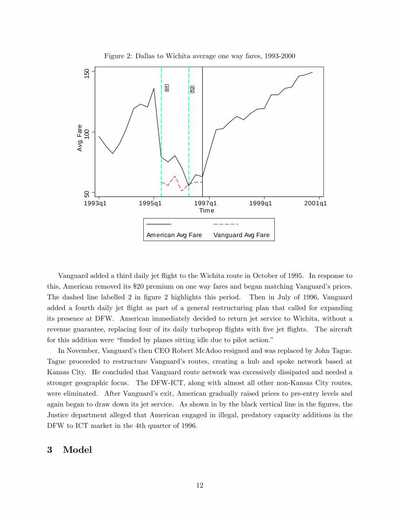
Figure 2: Dallas to Wichita average one way fares, 1993-2000
1 250
100
150
Avg
. Far
e
1993q1 1995q1 1997q1 1999q1 2001q1Time
American Avg Fare Vanguard Avg Fare
Vanguard added a third daily jet �ight to the Wichita route in October of 1995. In response to
this, American removed its $20 premium on one way fares and began matching Vanguard�s prices.
The dashed line labelled 2 in �gure 2 highlights this period. Then in July of 1996, Vanguard
added a fourth daily jet �ight as part of a general restructuring plan that called for expanding
its presence at DFW. American immediately decided to return jet service to Wichita, without a
revenue guarantee, replacing four of its daily turboprop �ights with �ve jet �ights. The aircraft
for this addition were �funded by planes sitting idle due to pilot action.�
In November, Vanguard�s then CEO Robert McAdoo resigned and was replaced by John Tague.
Tague proceeded to restructure Vanguard�s routes, creating a hub and spoke network based at
Kansas City. He concluded that Vanguard route network was excessively dissipated and needed a
stronger geographic focus. The DFW-ICT, along with almost all other non-Kansas City routes,
were eliminated. After Vanguard�s exit, American gradually raised prices to pre-entry levels and
again began to draw down its jet service. As shown in by the black vertical line in the �gures, the
Justice department alleged that American engaged in illegal, predatory capacity additions in the
DFW to ICT market in the 4th quarter of 1996.
3 Model
12

Figure 3: Dallas to Wichita seating capacity, 1993-2000
020
000
4000
060
000
8000
0S
eats
1993q1 1995q1 1997q1 1999q1 2001q1Time
American Turboprops American Jets
American Total Vanguard Capacity
In this section I introduce a dynamic model of price and capacity competition among airlines
competing in a nonstop market. There model has four important components. First, high marginal
cost/high quality, hub carriers and low marginal cost/ low quality, low cost carriers compete for
non-stop passengers by setting prices for their di¤erentiated o¤erings. Second, �rms must allocate
seating capacity to a route to serve passengers because they face capacity constraints in the form
of marginal costs that increase in the ratio of passengers to capacity. Third, moving capacity in
and out of markets is costly and these costs potentially di¤er for hub carriers and low cost carriers.
Finally, �rms face �xed costs of operating that can be avoided only if the �rm exits. These costs
may also di¤er across �rms.
Each �rm makes choices to maximizes its sum discounted sum of pro�ts. The last two features
of the model force rational �rms to be forward looking in the sense that they internalize the future
consequences of capacity, entry and exit decisions. I describe each component of the model and
then discuss equilibrium.
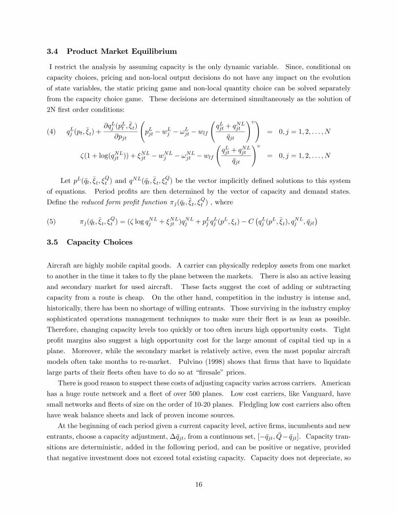
3.1 Local Demand
I assume each �rm produces a di¤erentiated product. Following Berry, Carnall and Spiller (2007), I
assume a nested logit speci�cation with the outside good (no �ight) in a nest and available products
13
in a second nest. The utility of consumer i from purchasing product j at time t is:
uijt = �pjt + �3Opresjt + �4Dpresjt + �5Stopjt + �j +��jt + �(�) + �ijt
Where pjt is the price of product j. The variables Opres and Dpres are a carrier�s total tra¢ c
at the origin and destination airports less the tra¢ c from the current market. They capture the
e¤ect of �airport presence�, as in Berry (1990). Travelers prefer to �y airlines, all else equal,
that o¤er more destinations due to, among others, the impact of frequent �ier miles and travel
agent commission overrides (see Berry 1990, or Borenstein 1990) . �j and ��jt are mean carrier
unobserved product quality and the deviation from this mean, assumed i.i.d across time and carriers.
These variables help account for unobservable factors like �ight frequency, ticket restrictions and
service quality. Berry (1994) and Berry, Levinsohn and Pakes (1995) discuss the usefulness of
these unobservable characteristics in properly accounting for substitution patterns. �ijt and �(�)
are terms capturing consumer speci�c heterogeneity. �(�) is the nesting term, re�ecting the fact
that there is a fundamental di¤erence between choosing whether or not to �y and choosing which
airline to �y. The structure of these two idiosyncratic terms is assumed to be such that the sum of
them is distributed as a type 1 extreme value random variable .
This di¤erentiated product assumption is vital since the goal of the model is to analyze com-
petition between a hub incumbent and a low cost entrant. Berry (1990) and Berry, Carnall and
Spiller (2007) show that passengers value the size of a hub carrier�s network and this superior
quality explains much of the hub premium, the premium a carrier is able to charge on itineraries
originating or terminating at its hub. Moreover, many of the cost reductions that low cost carriers
have been able to achieve, have come from elimination of unobservable service �frills�, presumably
at the expense of quality.
Let carrier j�s local demand state, ��jt, be de�ned as:
��jt = �pjt + �2Opresjt + �3Dpresjt + �4Stopjt + �j +��jt
Then, for a market of size M , the local tra¢ c demand function facing carrier j has the following
familiar form:
(1) qLj (pj ; p�j ; ��j;���j) =M
0B@ exp(�pj+��jt1�� )X
j0exp(
�pj0t+��j0t
1�� )
1CA0BB@
�Xj0exp(
�pj0t+��j0t
1�� )�1��
1 +�X
j0exp(
�pj0t+��j0t
1�� )�1��
1CCAWhich is the market size times the market share equation from the logit model with the outside
good in a nest and all other products in a nest.
14

3.2 Non-Local Demand
A complication arises because any given �ight between Dallas and Wichita transports both local
tra¢ c, passengers who originate at Dallas and whose �nal destination is Wichita, as well as non-
local tra¢ c, passengers traveling between a di¤erent origin and destination connecting over the
Dallas-Wichita route. Capacity decisions on a route depend on both types of traveler, however,
there is no obvious way to allocate the revenues and costs associated with non-local passengers to
the local route. I assume the revenue from non-local passengers is allocated to the route by a
function that depends on the total volume of non-local tra¢ c over the route and an exogenously
evolving state variable.
I assume the total demand for non-local service from carrier j over a route is given by the
inverse demand function pNLj (qNLjt ; �NLjt ), where q
NLjt is quantity of non-local tra¢ c and �NLjt is
carrier j�s non-local demand state. I specify the demand function as a constant elasticity form
pNLj (qNLjt ; �NLjt ) = � log qNLjt + �NLjt
The non-local revenues allocated to the route is then:
(2) pNLjt qNLjt = (� log qNLjt + �NLjt )q
NLjt
3.3 Variable Costs
Given its capacity level, a non-stop carrier faces a constant marginal cost of carrying passengers
plus an increasing �soft�capacity constraint. A nonstop carrier�s variable cost function is:
Cj(qLjt; q
NLjt ; �qjt) = (wLj + !
Ljt)q
Ljt(3)
+(wNLj + !NLjt )qNLjt
+
�wlf1 + �
� qLjt + q
NLjt
�qjt
!�(qLjt + q
NLjt )
!Ljt and !NLjt are mean 0 cost shocks identically and independently distributed over time and
across carriers. The form of the capacity constraint term�!lf1+�
��qLjt+q
NLjt
�qjt
��(qNLjt +q
NLjt ) is almost
identical to that used in Doraszelski and Besanko (2003) and Doraszelski et. al. (2008). The only
di¤erence is these papers set !lf = 1. The constraint is soft in the sense that a carrier is able
to violate the constraint though this cost may be high. A hard constraint would set the cost of
violating the constraint to in�nity. In this case a rationing rule would be required to calculate
equilibrium (if it exists). The parameter � determines how steeply marginal costs rise in a carrier�s
load factor, the ratio of a carrier�s tra¢ c to its capacity.
15
3.4 Product Market Equilibrium
I restrict the analysis by assuming capacity is the only dynamic variable. Since, conditional on
capacity choices, pricing and non-local output decisions do not have any impact on the evolution
of state variables, the static pricing game and non-local quantity choice can be solved separately
from the capacity choice game. These decisions are determined simultaneously as the solution of
2N �rst order conditions:
qLj (pt;��t) +
@qLj (pLt ;��t)
@pjt
pLjt � wLj � !Ljt � wlf
qLjt + q
NLjt
�qjt
!�!= 0; j = 1; 2; : : : ; N(4)
�(1 + log(qNLjt )) + �NLjt � wNLj � !NLjt � wlf
qLjt + q
NLjt
�qjt
!�= 0; j = 1; 2; : : : ; N
Let pL(�qt; ��t; �Qt ) and q
NL(�qt; ��t; �Qt ) be the vector implicitly de�ned solutions to this system
of equations. Period pro�ts are then determined by the vector of capacity and demand states.
De�ne the reduced form pro�t function �j(�qt; ��t; �Qt ) , where
(5) �j(�qt; ��t; �Qt ) = (� log q
NLj + �NLjt )q
NLj + pLj q
Lj (p
L; �t)� C�qLj (p
L; ��t); qNLj ; �qjt
�3.5 Capacity Choices
Aircraft are highly mobile capital goods. A carrier can physically redeploy assets from one market
to another in the time it takes to �y the plane between the markets. There is also an active leasing
and secondary market for used aircraft. These facts suggest the cost of adding or subtracting
capacity from a route is cheap. On the other hand, competition in the industry is intense and,
historically, there has been no shortage of willing entrants. Those surviving in the industry employ
sophisticated operations management techniques to make sure their �eet is as lean as possible.
Therefore, changing capacity levels too quickly or too often incurs high opportunity costs. Tight
pro�t margins also suggest a high opportunity cost for the large amount of capital tied up in a
plane. Moreover, while the secondary market is relatively active, even the most popular aircraft
models often take months to re-market. Pulvino (1998) shows that �rms that have to liquidate
large parts of their �eets often have to do so at ��resale�prices.
There is good reason to suspect these costs of adjusting capacity varies across carriers. American
has a huge route network and a �eet of over 500 planes. Low cost carriers, like Vanguard, have
small networks and �eets of size on the order of 10-20 planes. Fledgling low cost carriers also often
have weak balance sheets and lack of proven income sources.
At the beginning of each period given a current capacity level, active �rms, incumbents and new
entrants, choose a capacity adjustment, ��qjt, from a continuous set, [��qjt; �Q� �qjt]. Capacity tran-sitions are deterministic, added in the following period, and can be positive or negative, provided
that negative investment does not exceed total existing capacity. Capacity does not depreciate, so
16
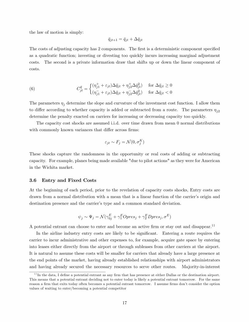
the law of motion is simply:
�qjt+1 = �qjt +��qjt
The costs of adjusting capacity has 2 components. The �rst is a deterministic component speci�ed
as a quadratic function; investing or divesting too quickly incurs increasing marginal adjustment
costs. The second is a private information draw that shifts up or down the linear component of
costs.
(6) C �qjt =
�(�+j1 + "jt)��qjt + �
+j2��q
2jt) for ��qjt � 0
(��j1 + "jt)��qjt + ��j2��q
2jt) for ��qjt < 0
The parameters �j determine the slope and curvature of the investment cost function. I allow them
to di¤er according to whether capacity is added or subtracted from a route. The parameters �j2determine the penalty exacted on carriers for increasing or decreasing capacity too quickly.
The capacity cost shocks are assumed i.i.d. over time drawn from mean 0 normal distributions
with commonly known variances that di¤er across �rms:
"jt � Fj = N (0; �Kj )
These shocks capture the randomness in the opportunity or real costs of adding or subtracting
capacity. For example, planes being made available "due to pilot actions" as they were for American
in the Wichita market.
3.6 Entry and Fixed Costs
At the beginning of each period, prior to the revelation of capacity costs shocks, Entry costs are
drawn from a normal distribution with a mean that is a linear function of the carrier�s origin and
destination presence and the carrier�s type and a common standard deviation.
j � j = N ( E0j + E1 Opresj +
E2 Dpresj ; �
E)
A potential entrant can choose to enter and become an active �rm or stay out and disappear.11
In the airline industry entry costs are likely to be signi�cant. Entering a route requires the
carrier to incur administrative and other expenses to, for example, acquire gate space by entering
into leases either directly from the airport or through subleases from other carriers at the airport.
It is natural to assume these costs will be smaller for carriers that already have a large presence at
the end points of the market, having already established relationships with airport administrators
and having already secured the necessary resources to serve other routes. Majority-in-interest
11 In the data, I de�ne a potential entrant as any �rm that has presence at either Dallas or the destination airport.This means that a potential entrant deciding not to enter today is likely a potential entrant tomorrow. For the samereason a �rm that exits today often becomes a potential entrant tomorrow. I assume �rms don�t consider the optionvalues of waiting to enter/becoming a potential competitor
17

agreements at some airports (including DFW) give the major carrier, e.g. American, a say in
proposed expansion plans, presumably leading to di¤erences in these costs across carriers beyond
even the observable di¤erences in presence. Ciliberto and Williams (2008) give a detailed discussion
of the determinants of these costs.
A �rm can choose to exit by choosing to sell o¤ all of its capacity. A carrier that chooses to
keep a positive level of capacity pays �xed costs in the following period that is the sum of two
terms. The �rst is a �xed cost of continuing operations and the second is proportional to the
amount of capacity the �rm holds
(7) �j + �q�qjt
This speci�cation re�ects the fact that at the route level certain expenses are �xed but avoidable,
i.e. costs that can not be subsumed into sunk entry costs because they can be avoided by exiting
or removing capacity. Also, many system or airport wide expenses, such as executive pay or
operations planning, have to be allocated to individual routes for the purpose of measuring the
performance of routes and making exit and capacity decisions. In its own decision accounting
system, American often allocates such expenses proportionally according to departures or other
tra¢ c measures. Though arguably arbitrary, since American bases decisions on these measures,
they presumably re�ect economic costs fairly well.
3.7 Bellman Equations
I restrict attention to Markov perfect equilibria of the above game. The reason for this is twofold.
First, most of the existing tools for equilibrium computation (e.g. McGuire and Pakes (1995, 2001))
as well as for estimation of structural parameters of the games (e.g. Aguirregabiria and Mira (2007)
, Pesendorfer and Jofre-Bonet (2005) , Bajari, Benkard and Levin (2007)) are designed for this class
of equilibria. Second, Markov perfection imposes some discipline on the analysis by restricting
dynamics to be driven only by fundamental or �payo¤ relevant� variables. This gives a �rmer
foundation to the analysis since belief related variables such as reputation are inherently di¢ cult to
measure and thus inherently more speculative. This restriction helps answer criticisms of the use
of modern strategic theory in the analysis of predation cases (see e.g Bolton, Brodley, and Riorden
2003 and the reply of Elzinga and Mills 2003). The �ip side of this strength is that the model does
not nest any of the theories that rely on asymmetric information as a driving factor.12
Time is discrete and in�nite. Within a period, inactive potential entrants see a random cost
of entry and decide whether to pay the cost and become active or disappear. All active �rms,
including entering �rms see a random shock to the cost of capacity adjustment and make capacity
adjustment decisions that take e¤ect in the following period. A �rm can choose to exit and
12Most theories of equilibrium predation rely on asymmetric information, e.g. Milgrom and Roberts (1983) Saloner(1989) Fudenberg and Tirole (1990) more cites. Cabral and Riorden (1995, 1997) o¤er a rationale, in the same spiritas the one o¤ered here, that does not rely on asymmetric info.
18

disappear by choosing to sell o¤ all its capacity. Firms then compete for passengers and realize
pro�ts for the period.
Each market is described by market states that evolve over time and type states which are time
invariant. In what follows I omit notation that shows the explicit dependence of values on these
type variables. Let S = (�q; ��t; �Qt ) Assuming that �rms follow Markov strategies, the value of a
�rm that has decided to remain active in the next period and has viewed its cost draw, "j , can be
written as the Bellman�s equation:
V Ij (S; "j) = max��qj2[��qj ; �Q��qj ]
�j(S)� �j � �q�qj � C �q(��q; "j) + �CVj(S;��qj)(8)
CVj(S;��qj) =
Z ZV I(S0; "0j) Pr(dS
0jS;��qj)F (d"0j)
Finally, the value of a potential entrant after viewing its sunk cost of entry and prior to seeing
its investment cost can similarly be written:
(9) V Ej (S; j) = max�j2f0;1g
�j
�� j +
ZV Ij (S; "j)F (d"j)
�In a Markov perfect equilibrium �rms policies are functions only of current payo¤ relevant
state variables. These include the market states for all competitor as well as private informa-
tion capacity shocks, entry cost draws for potential entrants, and scrap value draws for incum-
bents. I write these strategies, entry and capacity choice policies for each state as j(S; "j ; j) =
(�j(S; j);��qj(S; "j)).
De�nition 1 A Markov Perfect Equilibrium is: value functions ,V Ij , policy functions, j and
transition functions for all j 2 f1; : : : Ng such that:
V Ij (S; "j) = max��qj2[��qj ; �Q��qj ]
�j(S)� �j � �q�qj � C �q(��q; "j)(10a)
+�
Z ZV I(S0; "0j) Pr(dS
0jS;��qj)F (d"0j)
�j(S; j) = arg max�j2f0;1g
�j
�� j + �
ZV Ij (S; "j)F (d"j)
�(10b)
��qj(S; "j) = arg max��qj2[��qj ; �Q��qj ]
�j(S)� �j � �q�qj � C �q(��q; "j)(10c)
+�
Z ZV I(S0; "0j) Pr(dS
0jS;��qj)F (d"0j)
19

3.8 Discussion: Aggressive Pricing and Capacity Behavior
In the model, the intensity of price competition and period pro�ts are determined by the �closeness�
of �rms in characteristic and capacity space. The more similar �rms are in the characteristics,
including capacity, of their non-stop product, the greater the marginal impact of price changes on
quantity. The capacity constraint induces a similar e¤ect on the cost side. When �rms have
dissimilar capacity levels, the smaller �rms are unable to compete as aggressively on prices because
doing so incurs steeply increasing marginal costs. On the demand side the degree to which this
closeness matters is measured by the parameter �. High values of � correspond to high correlation
in utilities among consumers within a market and accordingly highly correlated choices. On the
cost side, the degree to which closeness matters depends on the parameter �. Higher values of �
correspond to harder capacity constraints and more steeply increasing capacity costs.
Pro�t functions exhibiting these features have been central in the literature of �rm and industry
dynamics (See Athey and Schmultzer (2001) or Doraszelski and Pakes (2007) for a review of these
results in the EP framework). Total industry pro�ts in these environments are greater when 1
�rm is dominant causing market equilibrium to tend to asymmetric structures with a dominant
�rm and occasional periods of intense competition when the laggard tries to become the market
leader. In the present model, with the possibility of exit, a dominant �rm anticipates these periods
of �erce competition and has incentive to preempt them by acting aggressively to cause losses and
potential exit by the laggard. The nature of asymmetries between the �rms determine the precise
nature of these incentives and the corresponding market dynamics.
4 Estimation
I will use the above model to simulate equilibrium in the Dallas to Wichita market under various
antitrust regimes. In this section I discuss how I estimate the game parameters to do these
simulations. The time series of relevant variables from an individual market, e.g DFW-ICT,
represents a single observation of a Markov perfect equilibrium. In order to do estimation and
inference, I need to observe equilibrium in many such markets. To this end, I construct a sample of
81 markets out of Dallas-Fort Worth and argue that these markets represent individual observations
of the same MPE.
4.1 Data and Sample Selection
The primary sources of data are from publicly available databases published by the Bureau of
Transportation Statistics. The �rst is origin and destination DB1B. The DB1B contains a quarterly
10% sample of all domestic origin and destination itineraries including number of connections,
carrier and fare paid. I keep those observations originating at Dallas-Fort Worth. I further keep
only round-trip fares and drop the lowest and highest 2.5% of fares in terms of fare per mile to avoid
20

frequent �ier tickets and possible coding errors. The DB1B lists three types of carrier for each
itinerary, ticking, reporting, and operating. I de�ne the carrier as the ticketing carrier and, when
there is more than one ticketing carrier, I de�ne the carrier as the listed as the ticketing carrier for
the segment out of DFW. I aggregate all remaining fares into passenger weighted, nonstop and
connecting fares for each market carrier quarter.
The second source, also from BTS, is the T100 Origin and Destination database. The domestic
T100 contains monthly data on tra¢ c for all origins and destinations within the U.S. for carriers
with annual revenues greater than $20 million. The variables include: carrier, O&D passengers,
seats, departures performed, departures scheduled, and distance for each route a carrier �ies. I
collect this data for all months from 1993-2000 and aggregate to make it quarterly. As with the
DB1B, I only include routes for which DFW is an origin or destination. I de�ne the capacity state
as the number of scheduled seats for a quarter. I construct the origin presence variable, Opresjt,
by summing all passenger tra¢ c originating at DFW for carrier j in period t less the tra¢ c from the
non-stop market in question. Similarly the destination presence variable, Dpresjtm, is constructed
by summing all of carrier j�s passenger tra¢ c originating at destination m in period t less the
tra¢ c from the non-stop market. Non-local tra¢ c on a route, qNLjt , is the T100 measure of total
tra¢ c over the route minus local tra¢ c. To exclude serial entry-reentry, likely driven by network
or seasonal factors, I de�ne carrier exit as a carrier�s reported DB1B passenger tra¢ c falling below
100 and entry as a carrier�s reported passenger total going above 100.13
Since my focus is on capacity, pricing, and entry/exit decisions in non-stop markets further
sample selection criteria must be used. Airline pricing and capacity decisions re�ect the complicated
network nature of the industry, particularly for hubbing carriers. I want to focus on markets and
�rms within those markets whose decisions are based on the same margins that model decisions
are based to make the same equilibrium assumption plausible. When network considerations are
�rst order relative to within market considerations this will not be true.
In order to concentrate on markets in which non-stop tra¢ c is the primary determinant of
pricing, I push competitors with with-stop service as well as competitors whose share of route
passengers is greater for a with-stop route than a non-stop route, into a competitive fringe and do
not analyze their decisions. By similar reasoning, I also only want to consider markets that are
not marginal with respect to providing any nonstop service. Entry and exit decisions in these,
usually small routes are also driven more by network considerations than by fundamentals in the
non-stop market. To deal with this I exclude markets in the bottom quartile of tra¢ c density.
Also I eliminate any markets that did not have any non-stop service at some point in the sample
period. This leaves 81 markets remaining in the sample. Table 2 shows some summary statistics
for the sample.
13The DB1B is a 10% sample so this corresponds to 1000 passengers on average.
21

Table 2: Summary Statistics (Excluding Southwest)variable mean s.d. min max
mean pop. (mn) 2.81 1.28 .645 6.65distance (miles) 788 552 175) 1660one way fare ($100) 1.74 .81 .34 5.80low cost fare 1.32 .53 .40 3.53AA fare 2.37 .86 .54 4.91nonstop �rms 2.2 1.02 1 5AA share .64 .16 .04 1LC share .18 .16 0 .954AA capacity per capita .028 .016 2.21e-4 .087low cost capacity p.c .0099 .0054 4.69e-5 .028Markets 81AA Non-stop Market-periods 2538Lowcost Nonstop periods 197Obs 12065
4.2 Estimation Strategy
I estimate the model in two stages. First, I estimate the parameters of the discrete choice demand
system. The demand system is a simple version of those expounded in Berry (1994) and Berry,
Levinsohn and Pakes (1995, BLP hereafter) and has been employed in many applications including
applications to air travel demand by Berry, Carnall, and Spiller (2006, BCS hereafter), Berry and
Jia (2008), and Aguirregabiria and Ho (2008). I then use these demand parameters to exploit the
static nature of the pricing game and recover �observed�marginal costs via a traditional markup
equation. Using these imputed costs I estimate the marginal cost function and the non-local price
equation by using the functional form for variable costs and the �rst order conditions from the
static game to form moment conditions.
The steps up to this point allow me to recover the realized variable pro�ts in the data. Es-
timation of the structural model, however, requires knowledge of variable pro�ts for all possible
points in the state space, whether or not they are observed. Being perfectly consistent with the
model would require re-solving the static pro�t game at each point in the state space (or at least
those that are reached with positive probability). This however is computationally demanding.
Instead I parametrize the pro�t function as a function of the state variables and estimate it from
the observed pro�ts, appealing to the assumptions of the model to argue consistency.
The �nal objects I estimate in the �rst stage are the dynamic policy and transitions functions.
Entry and Exit policies are estimated via probits on the market state variables and interaction
terms as well as concentration measures that are functions of the state variables. Capacity choice
policy functions are estimated via regressions of observed capacity choice on state variables and
interactions. The exogenous demand states and the growth rate of market size are assumed to
follow simple AR(1) processes
22
In the second stage I use the forward simulation estimator proposed by Bajari, Benkard and
Levin (2007) to estimate the capacity adjustment, �xed, entry, and exit costs. Starting with an
initial state in the data, I use the policy functions estimated in the �rst stage to simulate the
evolution of the market under the observed policy and a set of alternative policies. Estimation is
based on inequalities implied by the Markov perfect equilibrium assumption, i.e. the assumption
that the observed policies have higher (expected) returns than alternative policies. In the demand
and variable cost estimates, I am able to exploit the panel nature of the data to saturate the model
with �xed e¤ects to deal with unobserved heterogeneity, however the computational burden of the
second stage estimator increases dramatically in the number of parameters to be estimated. To
deal with this, I allow variable pro�ts, policies, transitions and dynamic cost parameters to vary
only according to whether a carrier is one of three types: American, Low Cost, or Other.
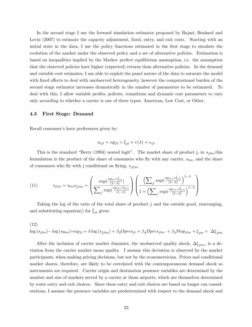
4.3 First Stage: Demand
Recall consumer�s have preferences given by:
uijt = �pjt + ��jt + �(�) + �ijt
This is the standard �Berry (1994) nested logit�. The market share of product j, in sjtm;this
formulation is the product of the share of consumers who �y with any carrier, stm, and the share
of consumers who �y with j conditional on �ying, sjtjm.
(11) sjtm = stmsjjtm =
0B@ exp(�pjt+��jt(1��) )X
j0exp(
�pj0t+�j0t(1��)
1CA0BB@
�Xj0exp(
�pj0t+��j0t
(1��)
�1��1 +
�Xj0exp(
�pj0t+��j0t
(1��)
�1��1CCA
Taking the log of the ratio of the total share of product j and the outside good, rearranging,
and substituting equation() for ��jt gives:
(12)
log (sjtm)� log (s0tm)=�pjt + � log (sjjtm) + �3Opresjt + �4Dpresjtm + �5Stopjtm + �jm + ��jtm
After the inclusion of carrier market dummies, the unobserved quality shock, ��jtm, is a de-
viation from the carrier market mean quality. I assume this deviation is observed by the market
participants, when making pricing decisions, but not by the econometrician. Prices and conditional
market shares, therefore, are likely to be correlated with the contemporaneous demand shock so
instruments are required. Carrier origin and destination presence variables are determined by the
number and size of markets served by a carrier at those airports, which are themselves determined
by route entry and exit choices. Since these entry and exit choices are based on longer run consid-
erations, I assume the presence variables are predetermined with respect to the demand shock and
23

are valid instruments. By similar reasoning, I ignore the potential selection issue arising from the
fact than carriers might condition entry and exit decisions on the demand shocks.
I follow BLP in constructing instruments for prices and conditional shares. They suggest
functions of the exogenous characteristics of competitors as instruments. The logic of identi�cation
is that these variables change the competitive environment, and shift markups accordingly, but are
uncorrelated with the carrier�s demand shock for the same reason that the carrier�s own exogenous
characteristics are uncorrelated with its own shock. I use the means and sums of opponent
origin and destination presences as well as the number of total competitors, number of connecting
competitors and number of low cost competitors as instruments. For comparison, Table 3 reports
utility parameters for the OLS as well as the IV speci�cation.
Table 3: Utility ParametersIV OLS
price($100) -0.6961 -.0488(0.2273) (.0040)
sjjfly 0.7281 .9581(0.1466) (.0025)
stop -0.3287 -.0919(0.4402) (.00913)
Dest. Pres.(millions) 0.0871 .0275(0.021) (.00375)
Origin Pres.(millions 0.0727 .0092(0.0729) (.0006)
Obs. 12065Equation includes carrier and market dumm ies. Instru-m ents: Sum of opponent presence and stop variab les,dummy for opponent entry
Having estimated the demand coe¢ cients, I can calculate residual demand elasticities for each
market, �jmt: Table 9 reports the elasticities implied by the estimates. Mean and median elas-
ticities are slightly higher than those found in previous studies (BCS, Berry and Jia 2008), which
�nd mean elasticities in the range of 1.5 to 2. The di¤erence arises likely because these studies
allow for a two type random coe¢ cient distribution and also do not aggregate fares. They �nd
evidence the two types have very di¤erent price sensitivities. Since my estimates are, in a sense,
averaging over the coe¢ cients of the di¤erent types, it is expected they might be biased toward
the larger group, i.e. price sensitive passengers. The results for Southwest are most troubling; the
average elasticity is below 1 implying negative marginal costs and a signi�cant fraction of markets
consistently display elasticities below 1. For this reason, I exclude Southwest in estimating the
marginal cost and variable pro�t function.
4.4 First Stage: Variable Costs
Combining the elasticities with the assumption that prices don�t in�uence the evolution of state
variables, I can back out marginal cost observations using the standard markup equation.
24

(13) cjtm = pjtm
�1� 1
�jmt
�The variation in the data is insu¢ cient to adequately identify both coe¢ cients in the capacity
cost term separately. Instead, I set � = 5 to re�ect the obvious hard constraint that a carrier can
never �y more passengers than it �ies seats as well as the observation that carriers �y planes at
less than capacity, which suggests increasing marginal costs below the capacity constraint. Also,
without price data for non-local tra¢ c, the constant marginal cost of non-local passengers and the
non-local demand state are not separately identi�ed. I therefore normalize this cost to 0. The
other cost and non-local pro�t parameters are estimated using the moments:
g1N (�C) =
1
T
1
M
TXt=1
MXm=1
1
Nm
NmXj=1
ZCjtm(cjtm � wLjm � wlf
qLjt + q
NLjt
�qjt
!5)(14)
g2N (�NL) =
1
T
1
M
TXt=1
MXm=1
1
Nm
NmXj=1
ZNLjtm(�(1 + log(qNLjt )) + �
NLjm � wlf
qLjt + q
NLjt
�qjt
!5)
Zc and ZNL are vectors of instruments. As with carrier local demand shocks, I assume �rms
know cost and non-local demand shocks when making output and pricing decisions, making load
factors endogenous. It has been documented that load factors correlate positively with the level of
competition in a market. My identi�cation strategy here then mirrors identi�cation of the utility
parameters. Zc and ZNL contain carrier market dummies, sums and means of opponent demand
characteristics, the number of total competitors, number of low cost competitors, and number of
connecting competitors. Within market variation in these variables should be uncorrelated with
deviations from own mean marginal costs since entry and network building decisions are based on
long run considerations, but will shift local quantities by changing the level of competition. These
variables also shift non-local tra¢ c by changing the marginal opportunity cost of non-local tra¢ c
but should not be related to the non-local tra¢ c price. The parameters (�C; �NL) are estimated
by minimize the stacked vector of these two moments. Table 4 shows the estimates excluding the
carrier market dummies.
The di¤erences in variable costs between American and low cost �rms is consistent with the
30-50% di¤erence in operating costs suggested by American�s own estimates over the period. The
estimates imply American�s average variable cost per available seat mile, a common measure of
costs, is around 3 cents. This is roughly 35% of the around 8 cent system wide total cost per
seat mile gleaned from accounting data, suggesting �xed costs are on the order of 65% of total
costs.
It is more di¢ cult to evaluate the plausibility of the non-local price parameters. Non-local
revenues must be allocated among the routes of an itinerary so even with price data evaluation
of the estimates is not feasible. Overall, however, the estimates seem reasonable. The median
25

Table 4: Variable Cost and Non-Local Price Parameters ($100)Coe¤. Standard Error
!lf 1.34 .250� -.180 .011Obs. 4571
Other param. mean std.dev.American !j .921 1.07
!lf
�qjt+Qjt
Kjt
�5.194 .153
Low Cost !j .572 .592
!lf
�qjt+Qjt
Kjt
�5.131 .114
Total !j 1.11 .823
!lf
�qjt+Qjt
Kjt
�5.135 .150
Instrum ents: Number of carriers, number of lowcost carriers, number con-necting products, Sum s and means of opponent demand characteristics
non-local price is $37 for American and $33 for low cost carriers. The distribution of these prices
is also fairly tight with an interquartile range of $30-$44 for American and $25-$38 for low cost
carriers.
4.5 First Stage: Variable Pro�ts
With estimates of variable costs, I can now recover period variable pro�t observations by plugging
the imputed costs into the variable pro�t equation
�jtm = pjtmqLjtm + (� log q
NLjtm + �
NL
jtm)qNLjtm � Cjtm
The mean and median variable pro�ts for American are $1,393,852 and $2,029,134 . For low cost
carriers the corresponding �gures are $718,819 and $895,720. Table 5 shows the statistics from the
distribution of these pro�ts broken out into the 3 component parts.
Table 5: Variable Pro�t BreakdownAmerican Low Cost Other
Mean (Millions) Frac Tot. Rev. Mean Frac. Tot. Rev. Mean Frac. Tot. Rev.Total Rev 4.06 1 1.57 1 1.86 1Local Rev. 2.09 .58 1.10 .74 1.13 .52Non-Local 1.45 .42 .387 .26 .731 .48Var. Cost 1.09 .16 .429 .21 .535 .25
Calcu lations use �tted variab le costs and non-lo cal demand. A ll ca lcu lations exclude Southwest
Ideally the static pro�t function would be recovered by solving the static game for each point
in the state space. This is computationally demanding so I opt to estimate the variable pro�t
function by �tting a �exible function of the state variables. Also, the computational burden of
the second stage estimator does not allow me to estimate di¤erent parameters for each market and
carrier. I therefore only allow pro�t functions to depend on the market state as well as the type
26

of each carrier, one of American, Low Cost, or Other. Speci�cally, I estimate using the following
moments:
(15) g3N (��) =
1
T
1
M
TXt=1
MXm=1
1
Nm
NmXj=1
f�type(Stm)(log(�jtm)� log(poptm)� f�type(Stm)�0)
Where f�type(Sjtm) is a vector of polynomial (quadratic) basis functions in a carrier�s own state
and means and sums of opponent�s states. Identi�cation relies on adequate variation in the state
variables and also relies heavily on the assumption the model is correctly speci�ed.
4.6 First Stage: Policy Functions
In a Markov Perfect equilibrium, equilibrium policies are functions of the �payo¤ relevant� state
variable alone. While, this restriction provides useful guidance, equilibrium policies are rarely
available in closed form. Without knowing the functional form the optimal way to proceed is
estimate the policies non-parametrically. Data limitations, however, preclude this. I choose to
estimate linear functions of the state variables and include relevant interaction terms.
Table 10, in the back of the paper, reports coe¢ cients from entry and exit probits. As found in
previous literature, origin and destination presence are very important predictors of entry likelihood
and to a lesser extent, exit likelihoods. As found by Berry (1990), entry by carriers who have no
presence at either market endpoint is very rare. In a few markets, there are carriers that appear
to repeatedly enter and exit the market. I assume that these are seasonal routes and exclude those
market carrier observations for which there are more than two total entries.
I estimate the capacity adjustment policy functions using a �exible polynomial speci�cation. As
in the variable pro�ts section, I estimate capacity policies for American, Low Cost, and Other type
carriers and treat mean carrier market costs as additional state variables. Formally, I estimate
capacity policies via the moments:
(16) g4N (���q) =
1
T
1
M
TXt=1
MXm=1
1
Nm
NmXj=1
f��qtype(Sjtm)(��qjtm � f��qtype(Sjtm)�
��q0)
Where f��q(Sjtm) is a vector of selected polynomial terms. As with the variable pro�t function
identi�cation rests on there being su¢ cient variation in the observed states and the model being
correctly speci�ed.
The estimation strategy taken here is inconsistent with the model in two ways. First, in the
model, the exit and capacity adjustment decisions are not distinct, a �rm exits by choosing to sell
o¤ all of its capacity. Here I estimate, and below use for simulation, separately estimated capacity
and exit policies. I do this to allow for potential misspeci�cation by allowing factors independent
of capacity costs to a¤ect exit decisions. The second inconsistency is the failure to correct the
capacity policy estimate for the truncation implied by the assumption that carrier�s can not sell o¤
27

more capacity than they currently hold. The consequences of these choices, however, are minimal.
The �tted probability of choosing to move to a negative capacity state is low for states observed in
the data and the probability of exit is high for low levels of capacity. In other words, together the
exit and capacity policy tell a carrier to move up or get out at low levels of capacity.
Finally Table 11, in the back of the paper, shows estimates of the transition functions for
the exogenous state variables. The transition functions are estimated as AR(1) processes. The
evolution of population is assumed to be governed by an AR(1) process on the rate of growth.
These estimates are used in simulation but not reported. The results show American has more
persistent local demand than its rivals but less persistent non-local demand. The lower persistence
in local demand for low cost carriers is likely due to the high seasonality and sensitivity to broader
economic conditions of price sensitive passengers, who compose a disproportionate share passengers
for low cost airlines.
4.7 Second Stage: Fixed,Entry and Capacity Costs
In this section I estimate the dynamic parameters of the game; the parameters describing capacity,
entry and exit costs. I do this by using a forward simulation estimator of the type suggested in
Bajari, Benkard, and Levin (2007). The estimator is based on the inequalities implied by the
above Markov Perfect equilibrium assumptions.
Abusing notation, de�ne the value of an incumbent prior to seeing it�s capacity cost shock and
with all competitors following an arbitrary policy pro�le by:
(17)
V Itype(Sj ) = E"F
��j(S)� �j � �q�qj � C �q(��qj(j); "j) +
ZV Itype(S
0j j) Pr(dS0j��qj(j); S;�j)�
Let � be a Markov perfect equilibrium strategy pro�le. Then for each carrier j, � must satisfy:
V Itype(Sj �j ;��j) � V Itype(Sj j ;��j) 8 j ; 8S
The second stage estimator exploits these inequalities by plugging in the estimated reduced form
policies for the equilibrium strategies
V Itype(Sj �j (�FS);��j(�FS); �SS ; �FS)� V Itype(Sj j ;��j(�FS); �SS ; �FS) � 0 8 j ; 8S
where �FS is the vector of parameters estimated in the �rst stage, �(�FS) denotes the reduced
from estimate of the equilibrium policy pro�le, and �SS is the vector of dynamic cost parameters
including the variance parameter describing the distribution of the linear capacity cost shocks.
From the above discussion, for any strategy pro�le, , the value function is linear function of
these parameters and has 3 terms. The �rst term is the expected discounted value of the �ow
pro�ts accruing to the �rm while it remains an active competitor. The second term is the expected
discounted stream of capacity adjustment costs the �rm incurs will incur. And the third term is
28

the expected discounted scrap value (entry cost) an incumbent (potential entrant) receives (pays)
upon exiting (entering) the market. All expectations are rational in the sense that they are taken
with respect to the true underlying transition functions, denoted � and strategies. Formally, the
value function for an incumbent can be written:
V Itype;m(Sj j ;�j ; �SS ; �FS) = E;��j(S; �FS)� E;�CIj (S; �SS ; �FS)� E;��j(S; �SS ; �FS)
Where,
E;��j(S; �FS)=E;�
" 1Xt==�
�t���(St; �FS)jS� = S
#(18)
E;�CIj (S; �; �FS) = �+1;typeE;�
" 1Xt==�
�t�� max(0;��qj(St; "jt; �FS))jS� = S
#(19)
+ �+2;typeE;�
" 1Xt==�
�t�� max(0;��qj(St; "jt; �FS))2jS� = S
#
+ ��1;typeE;�
" 1Xt==�
�t�� min(0;��qj(St; "jt; �FS))jS� = S
#
+ ��2;typeE;�
" 1Xt==�
�t�� min(0;��qj(St; "jt; �FS))2jS� = S
#
+ �EtypeE;�
" 1Xt==�
�t����qj(St; "jt; �FS)"jtjS� = S
#
E;��j(S; �; �FS)=E;�
" 1Xt==�
�t��If�qjt>0g�j jS� = S
#(20)
+ �qE;�
" 1Xt==�
�t��If�qjt>0g�qjtjS� = S
#(21)
The linear form of the value function makes the forming the simulated minimum distance estima-
tor simple. The terms inside the expectations depend only on the simulations using �rst stage
estimates. Bajari et al (2007) show how to form consistent estimates of these terms. The value
function can then be expressed as the product of the expected discounted value terms and the
vector of second stage parameters:
(22) Vtype(Sj j ;�j ; �SS ; �FS) =Wtype(S;j ;�j ; �FS) � �0SS
The Markov Perfect Equilibrium assumption implies there can are no pro�table deviations from
the observed policy. Here, the pro�tability of a deviant policy can be expressed as:
(23) g(x; �SS) = (Wtype(S;j ;��j ; �FS)�Wtype(S;
�j ;
��j ; �FS))�
0SS
29

The estimator chooses policies that minimize the pro�tability of these deviations. Formally, I
randomly draw a set of states and alternative policies from a distribution H to generate a set of
nk inequalities. The true parameters satisfy:
(24) �SS = argmin
ZIfg(X(k);�SS)>0gg(X
(k); �SS)2dH(X(k))
I follow Bajari et al. and form the sample objective function as:
(25) Qn(�SS) =1
nk
nkXk=1
Ifg(x(k);�SS)>0gg(x(k); �SS)
2
Using the estimated value of incumbency, I can estimate the distribution of sunk entry costs
using the fact that the entry policy satis�es:
(26) Pr(��jt = 1jS) = Pr( jt � V Ij (S; ))
The left hand side of the equation is the �rm�s entry policy, estimated in the �rst stage. I therefore
estimate the distribution by simulating the value function for K di¤erent states and estimating the
mean and standard deviation of j by:
(27) ( E0j ; E1 ;
E2 ; �
E) = �E= argmin
�EK�1
KXn=1
(��j (Sn)�(V Ij (Sn); �E))2
Capacity adjustment costs are identi�ed by comparing the capacity policies to the marginal
value of capacity, recovered in the �rst stage. The estimator asks: Which set of parameters
minimize the implied amount of money left on the table, where money on the table is the di¤erence
between the marginal value of capacity and the marginal cost of capacity. American adjusts
capacity more often and more quickly than its rivals, despite more persistent pro�tability states.
Under the assumption proportional �xed costs are the same across �rms, this implies the marginal
costs and the curvature of the cost function required to rationalize American�s capacity behavior
are lower than its rivals. In practical terms identi�cation is achieved through appropriate choices of
alternative policies for simulation. I choose alternatives by randomly perturbing the coe¢ cients of
the �rst stage capacity estimates to generate policies that respond more quickly or more sluggishly
to changes in the marginal pro�tability of capacity.
Fixed costs are identi�ed by comparing a �rm�s exit policy to the overall the variable pro�tability
of remaining in the market. Here, the amount of money left on the table is the value of the outside
option for a �rm that chooses to continue, normalized to zero, or the value of staying in the market
for a �rm that chooses to exit. Identi�cation of �xed costs is weak due to a small number of
exit observations. For American the problem is worse. Since American never exits, its �xed
costs are not identi�ed without the assumed parametric form of the probit model. Entry costs
30

Table 6: Dynamic Cost ParametersCoe¤.
Entry/Exit(Thousands of Dollars) AA �
LC 481.87Oth. 338.90
Opres(millions) -8.67Dpres(millions) -11.42
� AA 172.91LC 236.06Oth. 213.17
Fixed/Capacity�+1 AA 19.05
LC 26.60Oth. 28.11
��1 AA 18.37LC 24.44Oth. 21.47
�+2 AA 2.36e-4LC 3.10e-4Oth. 5.16e-4
��2 AA 1.51e-4LC 2.66e-4Oth. 1.01e-4
�q 11.596Estim ates based on simulations of 10000 alternative paths for each of 500states. E stim ates of W�s form ed by simulating paths until the averageconverges.
are similarly identi�ed by comparing the value of potential incumbency to the value of staying out
of the market. In the case of entry costs, not even the parametric form can identify American�s
costs. Since American is active in every market in the sample, there are no observations of it as a
potential entrant. Table 6 reports the dynamic cost parameter estimates.
The results imply median net pro�t margin for American is 18%, while for low cost �rms it is
15%. The corresponding mean values are 26% and 19%. Avoidable �xed costs, represent 13%
of median variable pro�ts,$1,393,852 for American and 33% of low cost median variable pro�ts,
$718,898. The �xed capacity costs parameter suggests a 150 seat jet costs a carrier that �ies
it once daily around $200,000 per quarter. In total, �xed capacity costs are around 57% of
median variable pro�ts for American and 50% for low cost carriers. Industry sources suggest
recent system wide margins, though highly cyclical, range around 8% for large network carriers
like American and around 10% for low cost carriers. The estimates are broadly consistent with
this after acknowledging DFW is a disproportionately large source of American pro�ts and local
markets provide higher margins.
Median Sunk Entry costs for low cost carriers are approximately 67% of median variable pro�ts.
This suggests entry costs are high after factoring in the implied sunk capacity costs of entry;
Entering �rms have to make relatively large capacity additions to cover �xed costs.
31

5 Antitrust Policy
In legal settings, the most commonly accepted de�nition of predation is the sacri�ce of short
run pro�ts that leads to the exit of competitors and, in so doing, leads to an increase in long
run pro�ts through enhanced market power. The current, Brooke Group, standard of predation
operationalizes this de�nition by employing a two part test. The �rst test requires evidence that
an alleged predator has priced below �a relevant measure of cost�. The second part requires a
plausible scenario of expected �recoupment through monopoly power, generally this is evidence of
(re)entry barriers, su¢ ciently high market concentration etc..
The origins of the cost based tests endorsed by Brooke Group14 is the rule and rationale proposed
by Areeda and Turner (1975). They argue a rational �rm will never set price below marginal cost
in the absence of predatory motives and therefore suggest this cost as the relevant standard. In
the absence of acceptable measures of marginal costs, they suggest using average variable costs as
a proxy for this ideal standard. The failure of the Brooke Group to take a stand on exactly which
measure of cost is relevant is indicative of the measurement issues acknowledged by Areeda and
Turner as well as the ensuing debate as to which if any justi�ed by a coherent economic theory.
Average variable costs, average total costs, average avoidable costs and incremental costs have all
been suggested as theoretically appropriate rules.
In this section, I use the estimated model to evaluate American�s liability in the Wichita market
according to various cost tests that have been suggested and applied since Areeda and Turner
(1975). These are average cost based tests, average avoidable cost, average total cost, and average
incremental cost, suitably reformulated to the non-price competition of the model I �nd that
American violates all of the proposed cost based tests in the Wichita market. I evaluate the
e¢ cacy of these tests by introducing a de�nition, following Ordover and Willig (1981) of predatory
incentives. In their de�nition, an act is predatory if it is optimal when its e¤ect on rival exit
behavior is considered but suboptimal otherwise.
After determining liability, I evaluate how the welfare consequences of predation, as de�ned,
compare to the welfare consequences of various remedies. While the American case was dismissed
prior to the consideration of appropriate remedy, I consider two possible remedies.15 The �rst
remedies I look at the proposed by the Department of Transportation Fair Competition Guidelines,
drafted at the height of policy concern about airline predation but never enacted. These rules
amount to limitations on the amount of capacity incumbent carriers can add in response to a rival
entry and I recalculate equilibrium under these restrictions to understand how these change the
distribution of market structures over time. Second, I calculate the treble damages implied by
each of the cost test violations by using the �tted residual capacity costs, recovered in estimation,
to simulate the model under the �but-for�that American was unable to violate the tests.14Brooke Group Ltd. V. Brown & Williamson Tobacco Corp. (1992) 509 U.S. 209-258.15See American�s Submission Regarding Remedy. The submission requested that the liability and remedy deter-
mination by conducted jointly. The court opted to take the government�s position and separate the two.
32

Figure 4: Dallas-Wichita 1993-2000: Model vs. Actual Prices
1993Q3 1994Q3 1995Q3 1996Q3 1997Q3 1998Q3 1999Q3 2000Q30
0.2
0.4
0.6
0.8
1
1.2
1.4
1.6
1.8
Time
Fare
($10
0)
AA ModelVanguard ModelAA actualVanguard Actual
5.1 Benchmark Model
To analyze the implications of predation policy in the Dallas-Wichita market, I �rst solve the model
in the absence of policy interventions. I assume there are 2 potential competitors, American and
a low cost competitor. I make this restriction because the data predict a low likelihood of entry
from any of the �rms with presence at Dallas or Wichita and the market is small.16
To solve the model I discretize the state space. I split each �rms capacity state into 21
equispaced intervals from 0 to 135,000. Each increment (6500 seats) is approximately equivalent
to �ying a small jet (150 seats) 3-4 times per week for a quarter. I discretize the local demand
state into 5 bins from -4.3 to -3.9, the range over which they vary in the data. I set the non-local
demand state to 2.04 for American and 1.80 for the low cost carrier. Constant marginal costs are
set to $54 for American and $34 for the low cost carrier.
I calculate the reduced form pro�t functions for each state by explicitly solving the system of �rst
order conditions (4) conditional on the state vector. Markov Perfect equilibrium, policy and value
functions for each player, is then computed using a Gauss-Seidel algorithm similar to that described
in Erickson and Pakes (1995). The capacity policy functions give the probability distribution over
16Experiments allowing for 3 competitors show a third �rm very rarely enters the market. Moreover, entry of twolow cost carriers into this market is unlikely and the estimation results for Other type carriers are implausible.
33

Figure 5: Dallas-Wichita 1993-2000: Model vs. Actual Capacities
1993Q3 1994Q3 1995Q3 1996Q3 1997Q3 1998Q3 1999Q3 2000Q30
1
2
3
4
5
6
7
8x 10⁴
Time
Sea
ts
AA ModelVanguard ModelAA ActualVanguard Actual
Figure 6:
next period states, where the underlying random variable is the private information capacity cost
shock. Similarly the entry policy for a potential entrant is a probability distribution over the
binary enter stay out choice. The underlying random variable is the sunk entry cost draw.
To simulate the model, I take draws from the estimated distributions of the private informations
and plug them into the computed policy functions. Figures 4 and 5 show the model time series
for prices and capacities using the observed values of exogenous shocks versus the actual series.
5.2 Assessing the E¢ cacy of Cost Based Liability Tests
The uncertainty in the model induces outcomes that will, ex-post, violate some cost test regardless
of the presence of predatory incentives. The appropriate formulations of tests therefore are based
on ex-ante beliefs and the information a carrier has when making its decision. The �rst rule I
consider, arguably the most stringent, is the average incremental cost test. From the perspective
of a �rm with �qj units of capacity the adjustment cost of increasing capacity is avoidable, however,
in periods subsequent to the increase pro�ts accrue to this decision. I assume the current period
cost of adjustment is the cost of adjustment amortized to the in�nite horizon. This test asks
34
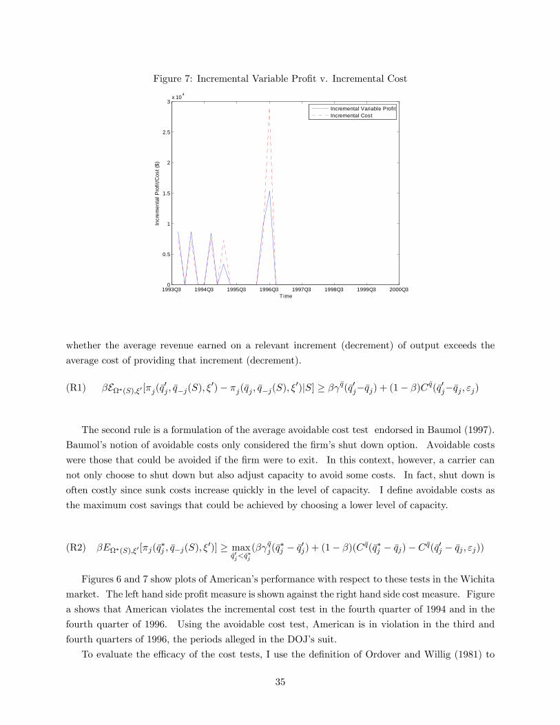
Figure 7: Incremental Variable Pro�t v. Incremental Cost
1993Q3 1994Q3 1995Q3 1996Q3 1997Q3 1998Q3 1999Q3 2000Q30
0.5
1
1.5
2
2.5
3x 10
4
Time
Incr
emen
tal P
rofit
/Cos
t ($)
Incremental Variable ProfitIncremental Cost
whether the average revenue earned on a relevant increment (decrement) of output exceeds the
average cost of providing that increment (decrement).
(R1) �E�(S);�0 [�j(�q0j ; �q�j(S); �
0)� �j(�qj ; �q�j(S); �0)jS] � � �q(�q0j��qj) + (1� �)C
�q(�q0j��qj ; "j)
The second rule is a formulation of the average avoidable cost test endorsed in Baumol (1997).
Baumol�s notion of avoidable costs only considered the �rm�s shut down option. Avoidable costs
were those that could be avoided if the �rm were to exit. In this context, however, a carrier can
not only choose to shut down but also adjust capacity to avoid some costs. In fact, shut down is
often costly since sunk costs increase quickly in the level of capacity. I de�ne avoidable costs as
the maximum cost savings that could be achieved by choosing a lower level of capacity.
(R2) �E�(S);�0 [�j(�q�j ; �q�j(S); �
0)] � max�q0j<�q
�j
(� �qj(�q�j � �q0j) + (1� �)(C �q(�q�j � �qj)� C �q(�q0j � �qj ; "j))
Figures 6 and 7 show plots of American�s performance with respect to these tests in the Wichita
market. The left hand side pro�t measure is shown against the right hand side cost measure. Figure
a shows that American violates the incremental cost test in the fourth quarter of 1994 and in the
fourth quarter of 1996. Using the avoidable cost test, American is in violation in the third and
fourth quarters of 1996, the periods alleged in the DOJ�s suit.
To evaluate the e¢ cacy of the cost tests, I use the de�nition of Ordover and Willig (1981) to
35

Figure 8: Variable Pro�t v. Avoidable Cost
1993Q3 1994Q3 1995Q3 1996Q3 1997Q3 1998Q3 1999Q3 2000Q30
2
4
6
8
10
12
14x 10
5
Time
Pro
fit/A
void
able
Cos
t ($)
Variable ProfitAvoidable Cost
measure predatory incentives. An act is predatory if it is optimal when its impact on its rivals exit
probabilities is considered but suboptimal otherwise. To formalize this, I follow Cabral and Riorden
(1997) and ask what behavior would be expected if American did not internalize the marginal impact
of capacity additions on Vanguard�s exit probability. To implement this I recalculate American�s
policy under the assumption that Vanguard�s exit probability remains constant across American�s
capacity states and assumes Vanguard�s actual behavior is exactly its observed behavior. Figure 8
shows the resulting capacity series plotted with the actual (benchmark model) series. The �gure
shows that predatory incentives were present throughout Vanguard�s tenure in the market. The
incremental cost test draws a false positive in the early period prior to Vanguard�s entry, and a
false negative in the 3rd quarter of 1996.
5.3 Remedies: Damages
Calculating damages, the lost pro�ts and consumer welfare resulting from illegal predatory acts,
requires constructing a counterfactual scenario for the market but for the predatory acts. I calculate
this counterfactual in 2 ways, both of which assume liability is determined by one of the two cost
tests and the relevant counterfactual is the market but for a violation of the test. In the �rst
approach, I consider equilibrium policies from the benchmark, unconstrained model and allow
American to re-optimize given it is prohibited from violating a given cost test. In the second
approach, I recalculate equilibrium under the restriction that American is unable to violate the
cost test in any period. Conceptually, the di¤erence between approaches is that in the former
the �rms behave as if the restriction is a one o¤ policy, i.e. they behave as if the probability of
36

Figure 9: A Measure of Predatory Incentives
1993Q3 1994Q3 1995Q3 1996Q3 1997Q3 1998Q3 1999Q3 2000Q32
2.5
3
3.5
4
4.5
5
5.5
6
6.5
7x 10⁴
Time
Sea
ts
NormalWithout "Pred.Incentive"
detection and punishment is 0, whereas in the latter, �rms behave as if violations of the test are
certain to be detected and punished. These can be seen as bounding cases of reality in which the
probability of detection and punishment is small but not 0.
The particulars of the American case are such that this distinction turns out to be a major one.
In the period of Vanguard�s exit it was hit with a large negative capacity cost shock, this is seen in
the steep decline in capacity in the period preceding its exit and in the same period as American�s
steep increase in capacity, and subsequent violation of the cost tests.17 The model predicts that
Vanguard continues to exit most of the time in the one o¤ scenario. In the recalculated equilibrium,
however, Vanguard�s behavior is much di¤erent exiting far less often.
Table 7 shows the results of these simulations. Overall the numbers are modest. In the one o¤
scenario, the incremental cost test gives a large improvement in Vanguard�s pro�ts but a decrease
in consumer welfare. This is because when Vanguard does not exit competition among the �rms is
quite dull. Vanguard�s exit probability is not a¤ected enough to o¤set the negative welfare impact
under the rule in the cases where Vanguard continues to exit. Vanguard�s exit policy is materially
17 It is likely that this is partially an artifact of the assumption that decisions are made simultaneously at thebeginning of a period. However, recall the exit decision was precipitated by a management change and overallrestructuring at Vanguard.
37

Table 7: Damages (Thousands of Dollars)"One O¤" Complete Enforcement
Incremental (R1) Avoidable(R2) Incremental AvoidableVanguard Pro�t Loss 45.67 29.79 123.52 103.80Consumer Welfare Loss -94.64 34.10 43.03 85.59Total Change -49.03 63.887 166.55 189.393xTotal Change -147.09 191.66 499.65 568.17
Figures are averages of 10000 simulated runs w ith cost sho cks drawn conditional on observed b ehavior. "One o¤"means that �rm s fo llow b enchmark equ ilibrium except in a p eriod w ith a cost test v io lation . "Complete Enforcem ent"m eans equ ilibrium probabilities are recalcu lated under the restriction that the cost test can not b e vio lated . Welfarechange is m easured ascompensating variation .
a¤ected under the complete enforcement scenario. The di¤erence in the damages �gures highlights
the subtleties of constructing an appropriate counterfactual.
5.4 Remedies: �Fair Competition Guidelines�
During the early 1990s entry and growth of the low cost segment was particularly rapid. By 1995,
they had, together, achieved a 20 percent share of the market.18 In the second half of the 1990s,
however, this growth began to slow, leading policy makers and the customers who had bene�ted
from the steeply falling fares to look for reasons why. One popular answer to the question was
predatory responses to low cost entry by big incumbents.
From late 1993 to late 1999 there were over 30 complaints of exclusionary, predatory conduct
�led by low cost carriers and investigated by the Department of Transportation. The problem was
considered severe enough that in April of 1998 the Department of Transportation circulated a draft
of proposed �Fair Competition Guidelines�for the industry, stating:
�We have concluded that unfair exclusionary practices have been a key reason that
competition from new low fair carriers has not been able to penetrate concentrated
hubs.�19
The FCG addressed what was perceived to be the typical �predatory�pattern: 1) A low cost
carrier enters a non-stop hub route of a dominant incumbent 2) The incumbent responds with steep
fare cuts and capacity increases. The Guidelines would initiate enforcement proceedings whenever
one of 3 rules, stated in terms of the incumbent�s passenger and capacity response relative to the
entrant�s capacity, was violated:
1. The major carrier adds capacity and sells such a large number of seats at very low fares that
the ensuing self-diversion of revenue results in lower local revenue than would a reasonable
alternative response,
2. The number of local passengers that the major carrier carries at the new entrant�s low fares
(or at similar fares that are substantially below the major carrier�s previous fares) exceeds
18Market share is de�ned as share of passenger revenue miles from Bureau of Transportation Statistics T1 database.19DOT Fair Competion Guidelines proposal p.7
38

the new entrant�s total seat capacity, resulting, through self-diversion, in lower local revenue
than would a reasonable alternative response, or
3. The number of local passengers that the major carrier carries at the new entrant�s low fares
(or at similar fares that are substantially below the major carrier�s previous fares) exceeds the
number of low-fare passengers carried by the new entrant, resulting, through self-diversion,
in lower local revenue than would a reasonable alternative response
In the context of the model these remedies amount to restrictions on the amount of capacity
that can be added to a route by the hub incumbent. Figures 9 and 10 show the time series plots for
model predicted prices and capacities and the predicted time series under the original benchmark
model as well as the counterfactual equilibrium with American able to add no more than 6500
seats in each period. Table 8 shows price, capacity and consumer welfare statistics under various
alternative restrictions. The FCG type remedies trade o¤ the increased consumer utility during
the predation period with the harm to consumer welfare if the monopolization is successful. As
evidenced by Table 8, the model predicts a net gain in consumer welfare would have been realized
had FCG type remedies been in place at the time of Vanguard�s entry.
Table 8: Actual and Expected Pro�t Changes Under FCG type Remedies(Thousands of Dollars)Compensating Variation LCC Pro�ts
Description Actual Change Expected Change Actual Change Expected ChangeCapacity Cap = 6500 152.12 25.09 219.64 211.11Capacity Cap =13000 160.70 79.93 134.62 115.94Capacity Cap = �q�j 177.14 87.14 9.88 66.89Figures are m eans of 10000 simulated runs of the model. Actual change: S imulated cost sho cks drawn conditional on b ehavior actuallyobserved . Exp ected change: S imulated cost sho cks drawn unconditionally. P ro�ts and calcu lated by the 12 quarter d iscounted sumof the p eriod values.
There are several problems with such retrospective analysis, however. First, the rules must
be enforced without knowledge of the ex post realizations of uncertainty, the capacity costs in the
model. If di¤erent realizations lead to di¤erent market outcomes than these alternative outcomes
have to be weighed. Second, if provisions are intended to protect e¢ cient, small, and �nancially
weak entrants like Vanguard, either selective enforcement is required or there is a risk that the
remedies can be exploited by �rms they are not intended to protect.
To address the ex ante uncertainty issue I use equilibrium policy functions to simulate the
distribution of market structures over time following the entry of Vanguard in the absence of the
remedies. Figure 11a-11c displays this distribution for two, eight, and 20 periods following entry
for the benchmark equilibrium. While there is a high probability that the incumbent responds
aggressively and drives the entrant out of the market, there is also a high probability that the
aggressive response is unsuccessful and the �rms compete vigorously for customers. Figures 12a-
12c show the same distributions under the assumption that American is restricted to 1 unit increases
in capacity. Clearly the restriction prevents American from monopolizing the market but it also
dulls competition in the intervening periods. The �Expected�columns of table 8 show the welfare
39

e¤ects of the FCG remedies from this, ex-ante, perspective. In this market, the chilling e¤ect of
predation policy is outweighed by the diminished likelihood of monopolization by driving a rival
out, as well as the increased likelihood of rival entry.
6 Conclusion
Since the U.S. airline industry was deregulated in 1978, one of the most important changes in
the industry has been the rise of the so-called low cost carriers. The growth of these carriers
has brought signi�cant bene�ts to customers, through steeply lower fares, in the markets they have
entered. Low cost has been equally damaging to the pro�tability of incumbent carriers, particularly
the large, hub and spoke carriers. These carriers, in the absence of low cost competition, enjoy
substantial markups on �ights to and from their hubs. Paradoxically, antitrust enforcers and
industry regulators have worried that low cost entry has stimulated too much competition in the
sense that incumbent responses in the sense that incumbent responses to that entry have been
predatory.
This paper has shown that this concern may be well founded. I propose a dynamic model of
airline competition, in which predatory behavior arises in the equilibrium of the game. Di¤erences
in cost structures between large, hub incumbents and small, low cost entrants cause these predatory
incentives to arise. Low cost carriers, with low marginal costs, set low prices and cut into the
pro�tability of the hub carriers. These hub carriers however have lower avoidable �xed costs, due
to prior sunk cost investments in their network, and are thus more committed to the market. Hub
carriers are then able to prey on their low cost rivals by making costly commitments of capacity to
a route.
While ruling out several interesting theories of predation, the structure of the model confers
some important advantages. Most important among these is its usefulness in interpreting real
market data. An incumbent�s principal tool for implementing a predatory strategy, capacity, is
easily measured using reliable, publicly available data. The Markov Perfect structure of the model
does not allow for predation based on reputation or other belief related phenomenon but provides
discipline by forcing predatory incentives to only rely on fundamental features of competition. It
also makes to model amenable to techniques for estimating the structural parameters.
Enforcement of predation standards in the airline industry, as in other industries, is di¢ cult.
This di¢ culty stems from the fact that predation is, by de�nition, a dynamic and strategic phe-
nomenon but there is a dearth of tools to think about it as such. Caution, therefore, generally
has to win out, as authorities fear attempting to prevent an ill-de�ned behavior risks distorting
incentives for vigorous competition. Applying the estimated model to a market from the Depart-
ment of Justice�s 2000 case against American Airlines, I �nd these problems are less severe than
the problem of predatory behavior itself. Commonly used static cost tests, which test for preda-
tory liability by comparing static revenue measures to static cost measures, are shown to capture
predatory incentives well when compared against a precise measure of predatory incentives. Also,
40

the results indicate, though predation remedies give rise to competition dulling incentives, they
also give rise to pro-competitive distortions, namely increased likelihood of low cost entry. I �nd,
on net, there is substantial scope for welfare improving policy.
This paper has explored only a few of the potential implications of the dynamic model. I
have used a single market to demonstrate the model, however, more complete answers to the
predation question require deeper analysis. For example predation policy must consider how
its impact changes with changing market conditions or across heterogeneous markets. Joskow
and Klevorcic (1979) propose a 2 part test for predation in which a court �rst determines if the
structural characteristics of a market make predatory behavior ex-ante plausible and then moves
on to apply liability tests. In the airline setting, relevant structural characteristics might include,
Business/Leisure traveller mix, market size, market distance, etc. Understanding how changes in
these variables a¤ect predatory incentives is important for understanding the potential consequences
of antitrust predation policy.
The economics highlighted here also have potential implications for other antitrust and industry
problems. For example, there are potential applications to analysis of airline mergers. In the
standard analysis, mergers that involve �rms that have limited route overlap, �end-to-end�mergers
such as the 2004 �barbell� merger of U.S. Airways and America West or the 2008 Delta and
Northwest merger, are considered fairly innocuous.20 The model I have presented casts doubt
on this assumption. It implies the such mergers may have implication for market entry through
changes in the cost structure of the merged �rm. I leave these questions for future research.
20The U.S. Airways-America West merger was refered to by the �rms as "operation barbell" because it mergedU.S. Airways considerable presence on the U.S. east coast with America West�s presence in the west.
41

References
[1] Aguirregabiria, V. and P. Mira �Sequential Estimation of Dynamic Discrete Games.�Econo-
metrica. 75(1). 2007: 1-53.
[2] Aguirregabiria, V and C. Ho �A Dynamic Oligopoly Game of the US Airline Industry: Esti-
mation and Policy Experiments�Working Paper, University of Toronto. 2008
[3] Areeda, P and D. Turner �Predatory Pricing and Related Practices Under Section 2 of the
Sherman Act.�Harvard Law Review. 88(4). 1975: 697-733.
[4] Athey, S. and P. Schmultzer. "Investment and Market Dominance." Rand Journal of Eco-
nomics. 32(1). 2001. 1-26.
[5] Bajari, P., L. Benkard, and J.Levin �Estimating Dynamic Models of Imperfect Competition.�
Econometrica. 75(5). 2007: 1331-1370.
[6] Bamberger, G. and D. Carleton. �Predation and the entry and exit of low-fare carriers.� in
Advances in Airline Economics: Competition Policy and Antitrust. D. Lee ed.. 2007
[7] Baumol, W. Panzar and R. Willig. Contestable markets and the theory of industry structure.
Harcourt Brace Jovanovic. New York. 1982.
[8] Baumol, W. �Predation and the Logic of the Average Variable Cost Test.�Journal of Law and
Economics. 39(1). 1996 49-72
[9] Benkard, L. "A Dynamic Analysis of the Market for Wide-Bodied Commercial Aircraft."
Review of Economic Studies. 71(3) 2003. 581 - 611
[10] Berry, S. "Estimation of a Model of Entry in the Airline Industry." Econometrica. 60(4). 1992
889-917
[11] Berry, S. "Estimating Discrete Choice Models of Product Di¤erentiation." Rand Journal of
Economics. 25(2). 1994 242-262.
[12] Berry, S., J. Levinsohn, and A. Pakes �Automobile Prices in Market Equilibrium�Economet-
rica. 63(4). 1995 841-890.
[13] Berry, S., P. Carnall, and M. Spiller �Airline hubs, costs, mark-ups and the implication of
customer heterogeneity.� in Advances in Airline Economics: Competition Policy and An-
titrust. D. Lee ed.. 2007. 183-214.
[14] Berry, S. and P. Jia. "Tracing the Woes: An Empirical Analysis of the Airline Industry." MIT
Working paper. 2008.
[15] Bersteneau, A. and P. Ellickson �Dynamics of Retail Oligopoly.� Duke University Working
Paper. 2004.
[16] Besanko, D. and U. Doraszelski. �Capacity Dynamics and Endogenous Asymmetries in Firm
Size.�Rand Journal of Economics. 35. 2004: 23-49.
42

[17] Besanko, D, U. Doraszelski, L. Lu, and M. Satterthwaite. �Lumpy Capacity Investment and
Disinvestment Dynamics.�Working Paper, Harvard University.2008
[18] Bolton, P.,J.F Bradley and M.H. Riorden �Predatory Policy: Strategic Theory and Legal
Policy.� Georgetown Law Journal. 88. 2000. 2239.
[19] Bolton, P. and J. Scharfstein. �A Theory of Predation Based on Agency Problems in Financial
Contracting.�American Economic Review. 80(1). 1990: 93-107
[20] Borenstein, S. �Hubs and High Fares: Dominance and Market Power in the US Airline Indus-
try.�RAND Journal of Economics. 20: 1989. 344-365.
[21] Borenstein, S. �Airline Mergers, Airport Dominance, and Market Power.�American Economic
Review Papers and Proceedings. 80: 1990. 400-404.
[22] Borenstein, S. �The Evolution of Airline Competition.� Journal of Economic Perspectives.
6(2). 1992: 45-73.
[23] Borenstein, S. �Hubs and High Fares: Dominance and Market Power in the U.S. Airline
Industry.�Rand Journal of Economics. 20(3). 1989: 344-365.
[24] Borenstein, S. and N.. Rose. �Competition and Price Dispersion in the US Airline Industry.�
Journal of Political Economy. 102: 1994. 653-683.
[25] Borenstein S. and N. Rose �How Do Airline Markets Work...Or Do They? Regulatory Reform
in the Airline Industry." NBER Working Paper #13452. 2007.
[26] Bork, R. The Antitrust Paradox. Basic Books. New York.1978.
[27] Cabral, L.M.B and M.H. Riorden. �The Learning Curve, Market Dominance and Predatory
Pricing.�Econometrica. 62(5). 1994: 1115-1140.
[28] Ciliberto, F. and J. Williams. �Limited Access to Airport Facilities and Market Power in the
Airline Industry.�University of Virginia Working Paper. 2008.
[29] Collard-Wexler, A. �Demand Fluctuations and Plant Turnover in the Ready Made Concrete
Industry�
[30] Doraszelski. U. and A. Pakes. �A Framework for Applied Dynamic Analysis in IO.�Harvard
University Working Paper. 2006.
[31] Edlin, A and J. Farrell. �The American Airlines Case: A Chance to Clarify Predation Policy.�
in J. Kwoka and L. White eds., The Antitrust Revolution: Economics, Competition, and
Policy. 2004. 502-531.
[32] Elzinga, K. and D. Mills. �Predatory Pricing and Strategic Theory.�Georgetown Law Journal.
89. 2001. 2475
[33] Erickson, R. and A. Pakes. �Markov-Perfect Industry Dynamics: A Framework for Empirical
Work�, Review of Economic Studies. 62. 1995. 53-82 .
43

[34] Fudenberg, D. and J. Tirole. �A Signal Jamming Theory of Predation.� Rand Journal of
Economics 17(3). 1986: 366-37.
[35] Genesove, D. and W. Mullin. �Predation and its rate of return: the sugar industry, 1887�
1914.�37(1). 2006. 47-69
[36] Goolsbee, A. and C. Syverson. �How Do Incumbents Respond to the Threat of Entry: Evidence
from the Major Airlines.�Quarterly Journal of Economics. Forthcoming.
[37] Gowrisankaran, G. and R. Town. �Dynamic Equilbrium in the Hospital Industry.�Journal of
Economics and Management Strategy. 6(1). 2004. 45 - 74
[38] Holmes, T. �The Di¤usion of Wal-Mart and the Economies of Density.� NBERWorking Paper
#13783, February 2008
[39] Ito, H. and D. Lee. �Incumbent Responses to Lower Cost Entry: Evidence From the U.S.
Airline Industry.�Working Paper. 2004.
[40] Joskow, P. and P. Klevorcic. �A Framework for Analyzing Predatory Pricing Policy.� Yale
Law Journal. 1979.
[41] Milgrom, P. and D.J. Roberts. �Predation, Reputation, and Entry Deterrence.� Journal of
Economic Theory. 27. 1982: 280-312.
[42] McGuire, P. and A. Pakes. �Computing Markov-Perfect Nash Equilibria: Numerical Implica-
tions of a Dynamic Di¤erentiated Product Model.�RAND Journal of Economics. 25. 1996.
555 589.
[43] McGuire, P. and A. Pakes �Stochastic Algorithms, Symmetric Markov Perfect Equilibrium,
and the �curse�of Dimensionality.�Econometrica. 69(5). 2001. 1261- 281.
[44] Ordover, J. and G. Saloner. �Predation, Monopolization, and Antitrust.� in R. Schmalensee
and R. Willig, eds., The Handbook of Industrial Organization, Amsterdam: North Holland.
1989. 537-596.
[45] Ordover, J. and Willig, R. �An Economic De�nition of Predation:Pricing and Product Inno-
vation�, Yale Law Journal, 91. 1981. 8-53.
[46] Pesendorfer, M. and P. Schmidt-Dengler. �Asymtotic Least Squares Estimators for Dynamic
Games.�The Review of Economic Studies. 75. 2008:901-928.
[47] Pulvino, T. �Do Asset Firesales Exist? An Empirical Investigation of Commercial Aircraft
Transactions.�The Journal of Finance. 53(3). 1998.
[48] Ryan, S. �The Costs of Environmental Regulation in a Concentrated Industry.�MIT Working
paper (2006)
[49] Saloner, G. �Predation, Mergers, and Incomplete Information.�Rand Journal of Economics.
18(2). 1987: 165-186.
[50] Scott-Morton, F. �Entry and Predation: British Shipping Cartels 1879-1929� Journal of
Economics and Management Strategy. 6(4). 1997. 679-724.
44
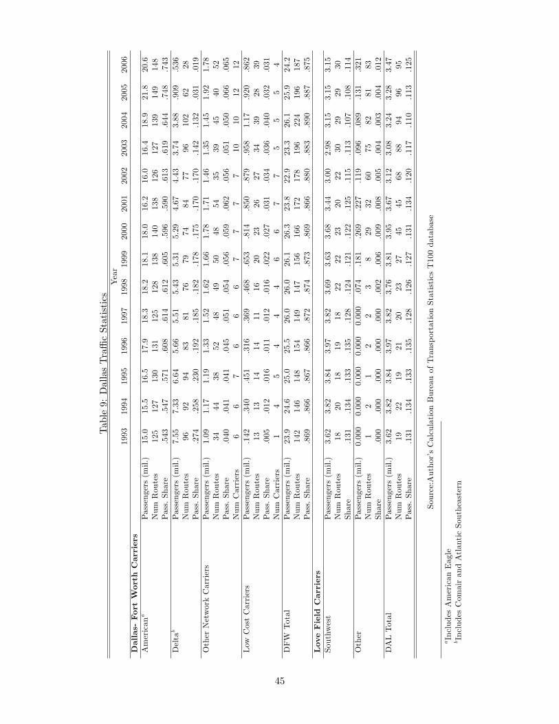
Table9:DallasTra¢cStatistics
Year
1993
1994
1995
1996
1997
1998
1999
2000
2001
2002
2003
2004
2005
2006
Dallas-FortWorth
Carriers
American
aPassengers(mil.)
15.0
15.5
16.5
17.9
18.3
18.2
18.1
18.0
16.2
16.0
16.4
18.9
21.8
20.6
Num
Routes
125
127
130
131
125
128
138
140
138
126
127
139
149
148
Pass.Share
.543
.547
.571
.608
.614
.612
.605
.596
.590
.613
.619
.644
.748
.743
Deltab
Passengers(mil.)
7.55
7.33
6.64
5.66
5.51
5.43
5.31
5.29
4.67
4.43
3.74
3.88
.909
.536
Num
Routes
9692
9483
8176
7974
8477
96102
6228
Pass.Share
.274
.258
.230
.192
.185
.182
.178
.175
.170
.170
.142
.132
.031
.019
OtherNetworkCarriers
Passengers(mil.)
1.09
1.17
1.19
1.33
1.52
1.62
1.66
1.78
1.71
1.46
1.35
1.45
1.92
1.78
Num
Routes
3444
3852
4849
5048
5435
3945
4052
Pass.Share
.040
.041
.041
.045
.051
.054
.056
.059
.062
.056
.051
.050
.066
.065
Num
Carriers
66
76
66
77
77
1010
1212
Low
CostCarriers
Passengers(mil.)
.142
.340
.451
.316
.369
.468
.653
.814
.850
.879
.958
1.17
.920
.862
Num
Routes
1313
1414
1116
2023
2627
3439
2839
Pass.Share
.005
.012
.016
.011
.012
.016
.022
.027
.031
.034
.036
.040
.032
.031
Num
Carriers
14
54
44
66
77
55
54
DFWTotal
Passengers(mil.)
23.9
24.6
25.0
25.5
26.0
26.0
26.1
26.3
23.8
22.9
23.3
26.1
25.9
24.2
Num
Routes
142
146
148
154
149
147
156
166
172
178
196
224
196
187
Pass.Share
.869
.866
.867
.866
.872
.874
.873
.869
.866
.880
.883
.890
.887
.875
LoveFieldCarriers
Southwest
Passengers(mil.)
3.62
3.82
3.84
3.97
3.82
3.69
3.63
3.68
3.44
3.00
2.98
3.15
3.15
3.15
Num
Routes
1820
1819
1822
2223
2022
3029
2930
Share
.131
.134
.133
.135
.128
.124
.121
.122
.125
.115
.113
.107
.108
.114
Other
Passengers(mil.)
0.000
0.000
0.000
0.000
0.000
.074
.181
.269
.227
.119
.096
.089
.131
.321
Num
Routes
12
12
23
829
3260
7582
8183
Share
.000
.000
.000
.000
.000
.002
.006
.009
.008
.005
.004
.003
.004
.012
DALTotal
Passengers(mil.)
3.62
3.82
3.84
3.97
3.82
3.76
3.81
3.95
3.67
3.12
3.08
3.24
3.28
3.47
Num
Routes
1922
1921
2023
2745
4568
8894
9695
Pass.Share
.131
.134
.133
.135
.128
.126
.127
.131
.134
.120
.117
.110
.113
.125
Source:Author�sCalculationBureauofTransportationStatisticsT100database
aIncludesAmericanEagle
bIncludesComairandAtlanticSoutheastern
45

1993Q3 1994Q3 1995Q3 1996Q3 1997Q3 1998Q3 1999Q3 2000Q30
0.5
1
1.5
2
2.5Figure Model Predicted Prices:FCG Ty pe Remedies
Time
Fare
($)
AmericanVanguard
Figure 9: Dallas-Wichita Model Predicted Price Series Capacity Cap = 6500 seats. 1993-2000
1993Q3 1994Q3 1995Q3 1996Q3 1997Q3 1998Q3 1999Q3 2000Q30
6500
13000
19500
26000
32500
39000
45500
56000Figure Model Predicted Capacities: FCG Ty pe Remedies
Time
Cap
acity
Uni
ts
AmericanVanguard
Figure 10: Dallas-Wichita Model Predicted Capacity Series. Capacity Cap = 6500 seats. 1993-2000
46

032500
6500097500
130000162500
032500
6500097500
130000162500
0
500
1000
1500
2000
2500
3000
Entrant Seats
Figure : Distribution of Capacities T=2 Periods After Entry
Incumbent Seats
Freq
uenc
y
032500
6500097500
130000162500
032500
6500097500
130000162500
0
500
1000
1500
2000
2500
Entrant Seats
Figure : Distribution of Capacities T=8 Periods After Entry
Incumbent Seats
Freq
uenc
y
032500
6500097500
130000162500
032500
6500097500
130000162500
0
1000
2000
3000
4000
5000
Entrant Seats
Figure: Distribution of Capacities T=20 Periods After Entry
Incumbent Seats
Freq
uenc
y
Figures 11a-11c: Benchmark (Unconstrained) Simulated distribution of market
capacity states. (a) 2 periods after entry. (b) 8 periods after entry. (c) 20
periods after entry.
47
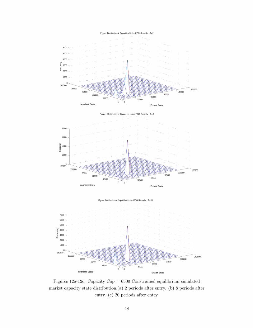
032500
6500097500
130000162500
032500
6500097500
130000162500
0
1000
2000
3000
4000
5000
6000
Entrant Seats
Figure: Distribution of Capacities Under FCG Remedy , T=2
Incumbent Seats
Freq
uenc
y
032500
6500097500
130000162500
032500
6500097500
130000162500
0
2000
4000
6000
8000
Entrant Seats
Figure : Distribution of Capacities Under FCG Remedy , T=8
Incumbent Seats
Freq
uenc
y
039000
6500097500
120000162500
039000
6800097500
120000162500
0
1000
2000
3000
4000
5000
6000
7000
Entrant Seats
Figure: Distribution of Capacities Under FCG Remedy , T=20
Incumbent Seats
Freq
uenc
y
Figures 12a-12c: Capacity Cap = 6500 Constrained equilibrium simulated
market capacity state distribution.(a) 2 periods after entry. (b) 8 periods after
entry. (c) 20 periods after entry.
48

Table 10: ElasticitiesCarrier Type mean s.d. perc.10 . perc.25 perc.50 perc.75 perc.90American Non-Stop -2.31 1.21 -3.94 -3.11 -2.30 -1.24 -.936
Connecting -6.08 2.44 -8.50 -7.36 -6.08 -4.66 -3.49Low Cost Non Stop -2.21 .926 -3.51 -2.82 -2.09 -1.57 -1.21
Connecting -3.48 1.13 -4.87 -4.09 -3.39 -2.67 -2.23Delta Non-Stop -2.88 1.48 -4.73 -3.80 -2.76 -1.65 -1.23
Connecting -4.81 1.22 -6.47 -5.55 -4.70 -3.95 -3.40Southwest Non-Stop -.669 .223 -1.01 -.793 -.615 -.514 -.415
Connecting -2.40 1.73 -4.89 -3.37 -2.00 -1.09 -.594Other Non-Stop -2.45 1.39 -4.27 -3.35 -2.36 -1.30 -.97
Connecting -4.14 1.82 -6.24 -4.99 -3.96 -3.05 -2.13
49
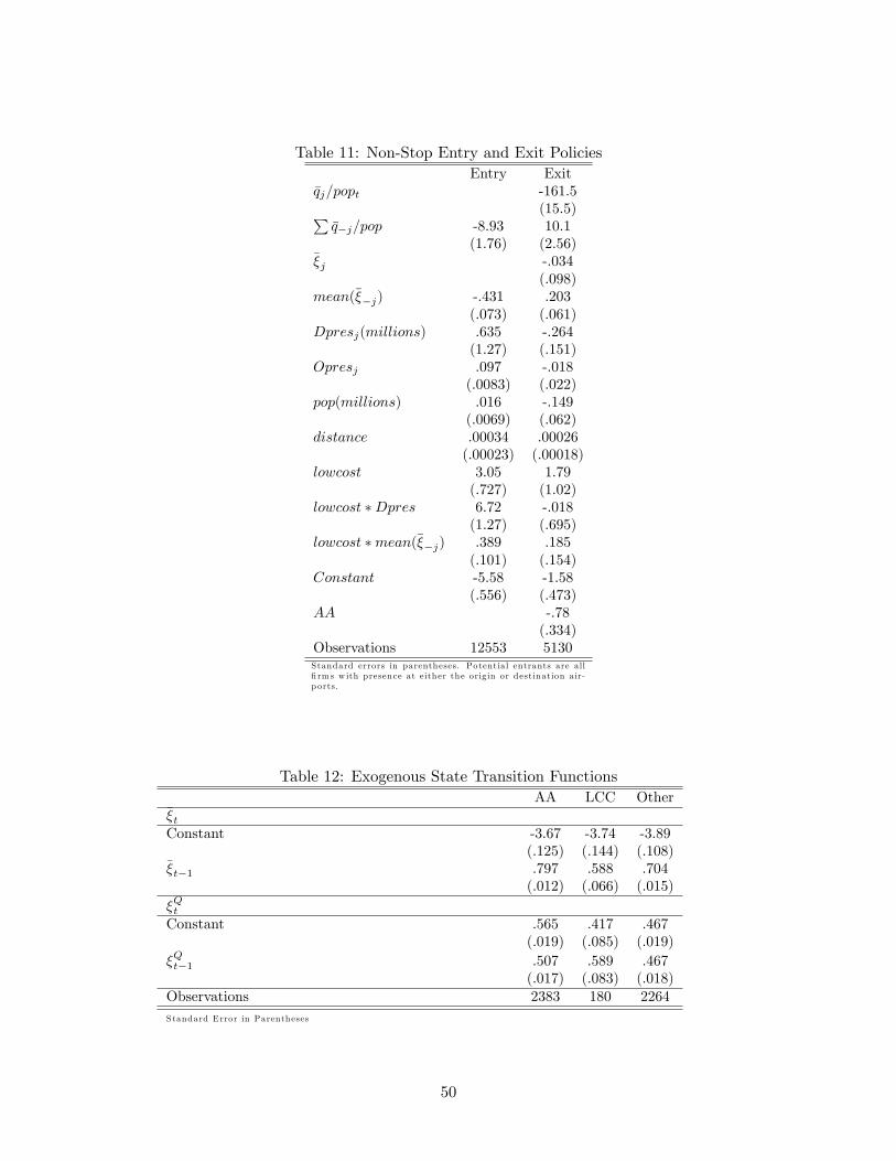
Table 11: Non-Stop Entry and Exit PoliciesEntry Exit
�qj=popt -161.5(15.5)P
�q�j=pop -8.93 10.1(1.76) (2.56)
��j -.034(.098)
mean(���j) -.431 .203(.073) (.061)
Dpresj(millions) .635 -.264(1.27) (.151)
Opresj .097 -.018(.0083) (.022)
pop(millions) .016 -.149(.0069) (.062)
distance .00034 .00026(.00023) (.00018)
lowcost 3.05 1.79(.727) (1.02)
lowcost �Dpres 6.72 -.018(1.27) (.695)
lowcost �mean(���j) .389 .185(.101) (.154)
Constant -5.58 -1.58(.556) (.473)
AA -.78(.334)
Observations 12553 5130Standard errors in parentheses. Potentia l entrants are all�rm s w ith presence at either the orig in or destination air-p orts.
Table 12: Exogenous State Transition FunctionsAA LCC Other
��tConstant -3.67 -3.74 -3.89
(.125) (.144) (.108)��t�1 .797 .588 .704
(.012) (.066) (.015)�QtConstant .565 .417 .467
(.019) (.085) (.019)�Qt�1 .507 .589 .467
(.017) (.083) (.018)Observations 2383 180 2264Standard Error in Parentheses
50