PREDATORY FISH POPULATION DYNAMICS AND DIET IN A

TRADITIONAL HAWAIIAN FISHPOND

A THESIS SUBMITTED TO THE GRADUATE DIVISION OF THE

UNIVERSITY OF HAWAIʻI AT MĀNOA IN PARTIAL FULFILLMENT

OF THE REQUIREMENTS FOR THE DEGREE OF

MASTER OF SCIENCE

IN

MARINE BIOLOGY

AUGUST 2018

By

Anela K. Akiona

Thesis Committee:

Erik C. Franklin, Chairperson

Brian N. Popp

Rob Toonen

Keywords: fishpond, population dynamics, diet, stable isotopes, barcoding

2

ABSTRACT

Overfishing and anthropogenic stressors have decimated Hawaiʻi’s coastal fisheries.

Traditional Hawaiian fishponds, or loko iʻa, are a low-impact and culturally significant food

source in the face of climate change and increased concerns over food security. Heʻeia fishpond,

on the windward side of Oʻahu, is currently trying to raise herbivorous fish as a local and

sustainable food source. It is therefore crucial to understand the population dynamics and diet of

predatory fish to assess their potential impact on the food production species. A mark-recapture

experiment (the Lincoln-Petersen closed population estimator with Chapman correction) was

conducted to estimate the population of predatory fish in the pond, and visual, genetic barcoding,

and stable isotope analyses were used to assess their diet. Catch-per-unit-effort data from

community fishing days were also utilized to examine trends in the relative abundance of

predator fishes. Sphyraena barracuda had the largest population in Heʻeia fishpond at 189

individuals, follwed by Caranx ignobilis (89) and C. melampygus (19), which reflects trends in

the CPUE from September 2016 – September 2017. Diets of the three species consisted mainly

of nearshore, estuarine fishes and crustaceans. We did not find evidence that the predators

consumed the herbivorous fishes typically raised as food, suggesting that they are either not

specifically targeted by the dominant predators in the fisphond or are such low population sizes

that they are not part of the predator’s diet. Based on these findings, we recommend maintaining

current strategies for management of Heʻeia Fishpond’s top predatory species.

3

ACKNOWLEDGMENTS

This work was supported by funding from the Hauʻoli Mau Loa Foundation, National

Science Foundation Graduate Research Fellowship Program, Kamehameha Schools ʻImi

Naʻauao Scholarship, Fernando Gabriel Leonida Memorial Scholarship Fund, and the Heʻeia

NERR (NOAA-NOS-OCM-2017-2005226).

I am extremely grateful to my advisor, Dr. Erik Franklin, for his support, encouragement,

and guidance throughout this project and my time at UH Mānoa. I am also grateful to my other

committee members, Drs. Brian Popp and Rob Toonen, for their expertise and feedback. I

would not have been able to complete such an ambitious project with my committe’s support at

every stage.

None of this would have been possible without the support of Paepae o Heʻeia. Thanks

especially to Hiʻilei Kawelo, Keliʻi Kotubetey, Loea Morgan, and Kanaloa Bishop for their

assistance in sample collection and coordination of volunteers for the tagging days. Many thanks

to the fishers that volunteered for my project and who let me measure their fish at Lā Holoholo.

I am also very grateful to Maia Kapur, Zack Oyafuso, and Dr. Megsie Siple for their

guidance and assistance with coding. Thanks as well to the Franklin Lab for all their support and

feedback over the last two years.

Mahalo nui loa to my family for their constant love, support, and encouragement.

Special thanks to my parents for assisting with every aspect of this project that they could, and

for always supporting me in everything I do; aloha au iā ʻoe.

4

TABLE OF CONTENTS

ABSTRACT .................................................................................................................................... 2

ACKNOWLEDGMENTS .............................................................................................................. 3

TABLE OF CONTENTS ................................................................................................................ 4

FIGURE LEGENDS ....................................................................................................................... 6

TABLE LEGENDS ........................................................................................................................ 7

INTRODUCTION .......................................................................................................................... 8

History of Hawaiian Fishponds .................................................................................................. 8

Approach ................................................................................................................................... 11

Chapter 1: Fishing for Science: Assessing predatory fish populations in Heʻeia Fishpond

....................................................................................................................................................... 13

ABSTRACT .................................................................................................................................. 13

INTRODUCTION ........................................................................................................................ 13

MATERIALS AND METHODS .................................................................................................. 15

Study site and species ............................................................................................................... 15

Catch-per-unit-effort ................................................................................................................. 16

Mark-release-recapture ............................................................................................................. 17

RESULTS ..................................................................................................................................... 19

Catch-per-unit-effort ................................................................................................................. 19

Mark-release-recapture ............................................................................................................. 24

DISCUSSION ............................................................................................................................... 26

Chapter 2: Diets of the predatory fish of Heʻeia Fishpond: Insights from stomach content

and stable isotope analyses ........................................................................................................ 29

ABSTRACT .................................................................................................................................. 29

INTRODUCTION ........................................................................................................................ 30

MATERIALS AND METHODS .................................................................................................. 32

Study site and sample collection ............................................................................................... 32

Stomach content analyses ......................................................................................................... 33

Bulk stable isotope analysis ...................................................................................................... 36

RESULTS ..................................................................................................................................... 39

Stomach content analyses ......................................................................................................... 39

Bulk stable isotope analysis ...................................................................................................... 46

DISCUSSION ............................................................................................................................... 50

5

LITERATURE CITED ................................................................................................................. 54

APPENDIX ................................................................................................................................... 59

6

FIGURE LEGENDS

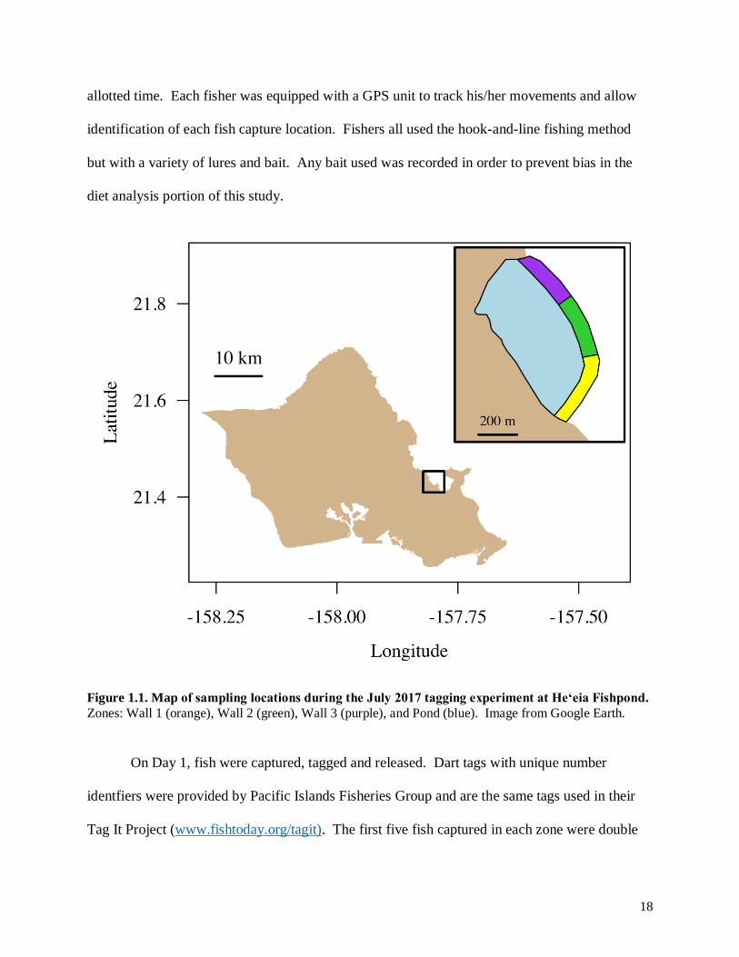
Figure 1.1. Map of sampling locations during the July 2017 tagging experiment at Heʻeia

Fishpond. ....................................................................................................................................... 18

Figure 1.2. Boxplots of fork length (mm) for each species caught at Lā Holoholo. .................... 21

Figure 1.3. Boxplots of mass for each species caught Lā Holoholo. ............................................ 22

Figure 1.4. Monthly mean predatory fish CPUE (pounds of fish per pole per hour) for each Lā

Holoholo with standard error bars shown. .................................................................................... 23

Figure 1.5. Monthly mean CPUE (pounds of fish per pole per hour) for each Lā Holoholo by

species. .......................................................................................................................................... 24

Figure 2.2. Collection locations of stable isotope samples from 2010 to 2011. .......................... 36

Figure 2.3. 𝛿15N and 𝛿13C values of all samples collected grouped by location. ...................... 39

Figure 2.4. Stacked barplots of numerically important prey (%N) for C. ignobilis (CAIG, n = 11)

and S. barracuda (SPBA, n = 29). ................................................................................................ 44

Figure 2.5. Stacked barplots of gravimetrically important prey (%W) C. ignobilis (CAIG, n =

11) and S. barracuda (SPBA, n = 29). .......................................................................................... 46

Figure 2.6. Modified Costello diagram showing the most important prey items in terms of prey

biomass (%W) and numerical importance (%N) for Sphyraena barracuda. ............................... 45

Figure 2.7. Modified Costello diagram showing the most important prey items in terms of prey

biomass (%W) and numerical importance (%N) for Caranx ignobilis. ....................................... 46

Figure 2.8. 𝛿15N and 𝛿13C values of all samples collected. ....................................................... 48

Figure 2.9. Isotopic niche breadth similarity of Caranx ignobilis (black ellipse) and Sphyraena

barracuda (green ellipse) in Heʻeia Fishpond. .............................................................................. 49

Figure 2.10. Estimated median contibution of prey taxa to the diet of Caranx ignobilis (white

papio) and Sphyraena barracuda(barracuda) in Heʻeia Fishpond. .............................................. 50

7

TABLE LEGENDS

Table 1.1. Catch number (n) and mean fork length (FL) and standard deviation (SD) of the top

three species caught at Lā Holoholo and by Paepae o Heʻeia staff from December 2015 to

January 2017. ................................................................................................................................ 16

Table 1.2. Summary of information collected at Lā Holoholo from September 2016 to September

2017............................................................................................................................................... 20

Table 1.3. Total numbers of fish marked on Day 1 (M), fish marked and unmarked caught on

Day 2 (n), and fish recaptured on Day 2 (m) for each species across the entire fishpond. ........... 25

Table 1.4. Number of fish marked on Day 1 (M), number of fish marked and unmarked caught

on Day 2 (n), and number of marked fish caught on Day 2 (m) by species for each zone. .......... 25

Table 2.1. Summary table of predatory fish species examined for stomach contents in Heʻeia

Fishpond. ....................................................................................................................................... 40

Table 2.2. Asymptotic species richness estimates with 95% confidence intervals. .................... 41

Table 2.3. Prey table for Caranx ignobilis (CAIG) and Sphyraena barracuda (SPBA)................ 41

Table 2.4. Summary of prey found in Caranx melampygus individuals as prey numbers and

weights. ......................................................................................................................................... 42

Table 2.5. Mean and standard deviation (SD) of Caranx ignobilis and Sphyraena barracuda bulk

𝛿15𝑁 and 𝛿13𝐶. .......................................................................................................................... 47

Table A1. Stable isotope values for all prey taxa collected in Heʻeia Fishpond from 2010-2017.

....................................................................................................................................................... 59

Table A2. Sequence identifications, length, and percent similarities from the BOLD and

GenBank (with ACCN) databases. ............................................................................................... 67

Table A3. Fork length (mm), total length (mm), weight (g), and stomach fullness (g) of all fish

utilized for diet analyses. .............................................................................................................. 70

Table A4. Prey taxa, digestion state, length (mm), weight (g), and total weight (g) of all prey

items found.................................................................................................................................... 73

8

INTRODUCTION

The State of Hawaiʻi, the most isolated archipelago on the planet, is home to nearly 1.43

million people. Because of this extreme isolation, the State imports nearly 90% of its food and

energy resources from the mainland USA and other parts of the world (Keffer et al. 2009). The

nearshore fisheries face not only overexploitation, but many anthropogenic stressors as well

(Friedlander and DeMartini 2002).

Rising regional and global demand for fish and fishery products may fall short of wild

fishery production capabilities. Aquaculture may be able to meet some of these demands while

alleviating pressure on wild stocks (Naomasa et al. 2013). Local aquaculture production

provides access to fresh seafood while avoiding high import costs and without diminishing

freshness or quality. The local market in Hawaiʻi exhibits favorable signs for increased

aquaculture production. Hawaii consumers demonstrate an increasing demand for seafood with

consumption rates that are double the national average (Loke et al. 2012).

The aquaculture industry in Hawaiʻi is fast-growing and has been viewed as an important

replacement for imported seafood. In 2010 it was a $30 million industry, doubling its value over

the previous 10 years (USDA 2011). Aquaculture grew an additional 250% 2010 to $76 million

in 2015 (USDA 2016). However, only 12% of the aquaculture farms in 2007 were classified as

efficient (Kim et al. 2015), showing ample opportunity for additions to the aquaculture industry

in Hawaiʻi.

History of Hawaiian Fishponds

Traditional Hawaiian fishponds, or loko iʻa, are an example of ancient aquaculture that

can provide a sustainable and pragmatic solution to sustainability challenges and biosecurity

9

concerns in the face of climate change. Since before the 13th century, loko iʻa served as a living

food pantry that could be harvested from year round during food shortages or periods of poor

fishing (Farber 1997, Sato and Lee 2007). Loko iʻa were typically built along the shore where a

freshwater stream emptied into the ocean. The brackish water and shallow depths of these

estuarine environments produced optimal conditions for the cultivation of algae (Apple and

Kikuchi 1975, Kelly 1994). The combination of rich algae growth, along with the right species

of herbivorous fish, gave Hawaiians a protein source that was 100 times more efficient than in

the natural estuarine food chain (Kelly 1994).

Fishpond management focused on the cultivation of herbivorous fish such as (in order of

importance): Mugil cephalus (mullet or ʻamaʻama), Chanos chanos (milkfish or awa), and

Polydactylus sexfilis (threadfin or moi) (Vockeroth 1981). Occasionally predators entered the

pond, but as long as their numbers were kept low they could not significantly impact the

population of herbivores (Sato and Lee 2007).

Building a fishpond was a community undertaking—large loko iʻa required upwards of

10,000 men to complete construction (Kamakau 1976, Farber 1997); similarly, maintaining a

fishpond required the help of many hands. However, Hawaiʻi’s rapidly changing socioeconomic

climate in the 1800’s led to a decline in the number of operated fishponds. With the advent of

more lucrative trades, such as sandalwood trading and whaling, the Great Māhele land division

of 1848, and depopulation from diseases, loko iʻa maintenance declined (Farber 1997). Lower

labor costs made it cheaper to import fish than to raise them, and short-term gains from ocean

fishing became more enticing than the long-term investment of operating the loko iʻa (Farber

1997).

10

Out of 488 loko iʻa statewide, 178 were located on Oʻahu. Around 1900, fishponds

accounted for almost 10% (682,484 pounds) of the fish caught in Hawaiʻi, of which 560,283

pounds were from Oʻahu alone (Cobb 1902). In 1994, only 6 were still operating commercially

statewide, with a yield of just 31,639 pounds valued at $68,911 (Farber 1997). The Hawaiian

Renaissance of the 1960s and 70s saw a renewed interest in loko iʻa, including at Heʻeia

fishpond, located in Kāneʻohe Bay. A 1972 proposal to develop Heʻeia Fishpond into a boat

harbor was met with strong protest (Farber 1997), and this community interest helped to lay the

foundation for the pond’s current restoration and the founding of Paepae o Heʻeia, the fishpond’s

managing organization.

Heʻeia Fishpond is one of only a handful of traditional Hawaiian fishponds that are still

operational and working towards (or currently) commercially producing fish. Fishponds are

grossly understudied even though they represent integrated multi-trophic aquaculture that is

culturally significant, relatively low-cost, and low-impact. Estimates of loko iʻa yields vary from

175 to 275 pounds per acre per year (Wyban 1992, Farber 1997) up to 350 pounds per acre per

year (Apple and Kikuchi 1975). This has the potential to provide a substantial amount of food to

Hawaiʻi residents.

It will take several years before the native herbivores at Heʻeia Fishpond are ready to be

harvested, but in the meantime it is important to understand how predators might be affecting

their populations. This raises some questions about the population dynamics of the dominant

predatory fish species in the loko iʻa: Caranx melampygus (ʻomilu), C. ignobilis (white papio),

Sphyraena barracuda (kākū).

11

Approach

The objective of this thesis is to assess the population dynamics and dietary preferences

of the three main predatory fish species in Heʻeia Fishpond, with a focus on their interactions

with and potential impact upon the herbivorous fish traditionally raised in these systems. The

results could have implications for how the fishpond in managed, and has potential to be utilized

by fishponds throughout Hawaiʻi.

Chapter 1: Fishing for Science: Assessing predatory fish populations in Heʻeia Fishpond

directly and indirectly estimates the abundance of predatory fish in the pond using conventional

mark-release-recapture methods and CPUE from community fishing events. Our findings

indicate that the predatory fish population in Heʻeia Fishpond is relatively low, when spread out

over the pond’s 88 acres. We estimate the total population of the three dominant predatory fish

to be less than 300 individuals, with evidence for seasonal changes in population numbers. This

demonstrates that fishing effort may be best directed during warmer summer months, when fish

catches are generally higher, although current management policies seem to be sufficient to keep

population sizes low.

Chapter 2: Diets of the predatory fish of Heʻeia Fishpond: Insights from stomach content

and stable isotope analyses utilizes visual gut content techniques, genetic barcoding, and stable

isotope analyses to determine whether the dominant fishpond predators are targeting the

herbivorous fish traditionally raised and harvested for consumption. Genetic barcoding greatly

improved the identification of prey taxa, many of which were greatly digested. The

incorporation of bulk tissue stable isotope methods and Bayesian mixed modeling allowed for a

more holistic picture of the predators’s dietary preferences, in addition to the ‘snapshot’ picture

12

provided by more traditional methods. We did not identify any of the herbivorous fish species of

interest in any stomachs, which suggests that the predatory fish impact upon these species is

minimal. This study has implications for the management of traditional Hawaiian fishponds

around the State.

13

Chapter 1: Fishing for Science: Assessing predatory fish populations in

Heʻeia Fishpond

ABSTRACT

Mark-recapture and catch-per-unit-effort (CPUE) methods are fundamental tools of

fisheries management. We used both methods to assess the population of predatory fish in

Heʻeia Fishpond, which is a traditional Hawaiian fishpond that is working towards producing

herbivorous fish. CPUE (# fish/pole/hour) was calculated from monthly community fishing

events that were held from September 2016 to September 2017. Caranx ignobilis was caught

most frequently during these events, with overall catches appearing to be higher during warmer,

summer months, although this relationship was not statistically significant. Additionally, a

mark-recapture experiment was conducted in July 2017 to directly estimate the number of

predatory fish in the pond. Sphyraena barracuda was the most abundant (190 individuals),

followed by C. ignobilis (89), and C. melampygus (19). It is likely that the most abundant

species changes throughout the year. All individiuals captured for all three species were smaller

than mean length at maturity, indicating that the predatory fish populations are largely immature.

Continued research and additional mark-recapture studies will greatly improve our understanding

of the population dynamics of the dominant fishpond predators.

INTRODUCTION

Making unbaised abundance estimates is a critical part of successful fisheries

management. Mark-recapture studies are used to make estimates of population size, survival and

rectuitment, to learn about a population’s response to management protocols, and to validate

14

population indices used for long-term monitoring (Gwinn et al. 2011, Peterson et al. 2015, Ruetz

et al. 2015). These methods have been used most successfully to estimate the abundance of

terrestrial animals or of fishes in enclosed lakes, but they can be used for marine species in

confined areas (Jennings et al. 2001). Mark-recapture methods for two sampling periods rely on

marks being applied to a subset of the target population during the first sampling event, then

using the ratio of marked to unmarked fish captured during the second sampling event to

estimate abundance (Seber 1973).

One such model is the Lincoln-Petersen mark-recapture model with Chapman correction,

which is unbiased at low sample sizes, particularly when the number of recaptures = 0 (Chapman

1951, Seber 1973). Capture probability (q) refers to the likelihood that a fish is captured during

a sampling event, and we consider the case where sampling is conducted via hook-and-line

fishing in a fishpond. This model has several assumptions that must be met (Pine et al. 2012):

(1) The population is closed both physically (i.e. no immgration or emigration) and

demographically (i.e. no recruitment or mortality);

(2) q is the same for marked and unmarked fish;

(3) Marks are not lost or undetected;

(4) Marked fish mix randomly with the population when released; and

(5) Marking does not affect fish behavior or vulnerability.

Oftentimes, it is not possible to directly estimate fish populations, and therefore relative

abundance is a widely used tool in fisheries stock assessment and management. An abundance

index is used to monitor stock status for conservation to fine-tune population dynamics models

(Geromont and Butterworth 2015, Tu et al. 2015). Since much of the data available is fishery-

dependent, catch-per-unit-effor (CPUE) is calculated by accounting for various factors (such as

15

time) that are not constant between samples (Maunder and Punt 2004). While mark-recapture

models provide direct estimates of population size, CPUE only demonstrates trends in catches

which may or may not be related to population abundance (Stenseth 2002).

Traditional Hawaiian fishponds are estuarine environments enclosed by a rock wall,

where herbivorous fish such as Mugil cephalus, Chanos chanos, and Polydactylus sexfilis were

raised for consumption by the local community. In 1965, a large flood destroyed a 200 ft.

portion of Heʻeia Fishpond’s wall, allowing fish to transit freely in and out of the pond. The

hole was repaired in 2015, but after 50 years of being open to the ocean, it is unclear how many

predatory fish remain in the pond. As the fishpond managers work to cultivate the herbivorous

fish, it is important to understand what local factors may be affecting their populations.

In the present study, we estimated the population sizes of the three dominant predatory

species in Heʻeia Fishpond using the Lincoln-Peterson model with Chapman correction. Our

research objective is to provide meaningful scientific results to managers of Hawaiian fishponds

that support sustainable food production through the utilization of mark-release-recapture

methods and catch per unit effort (CPUE) data. These results will specifically benefit the

community of fishers, seafood consumers, and caretakers of Heʻeia Fishpond, with potential

application to fishponds throughout the islands.

MATERIALS AND METHODS

Study site and species

This study was conducted at Heʻeia Fishpond, an 88 acre traditional Hawaiian

aquaculture system located in Kāneʻohe Bay on the windard side of Oʻahu (21°26'8.33"N,

157°48'27.28"W). The 88 acre pond is surrounded by a 1.3 mile stone wall, or kuapā, built of

16

basalt boulders and filled with coral rubble. Built into the kuapā are mākāhā, or sluice gates,

which control the flow of water and fish into and out of the pond (Farber 1997). Fishponds are

traditionally built on shallow reef flats no more than 10-15 ft deep where algae, or limu, can

easily grow. Heʻeia Fishpond is a brackish water environment with freshwater input coming

from nearby Heʻeia stream and submarine groundwater discharge (Leta et al. 2016).

The study species were determined from previous hook-and-line catch records from the

fishpond from December 2015 to January 2017. Caranx ignobilis, C. melampygus, and

Sphyraena barracuda had the three highest catch numbers (Table 1.1). The next highest

predatory species captured was Lutjanus fulvus (35 individuals).

Table 1.1. Catch number (n) and mean fork length (FL) and standard deviation (SD) of the top

three species caught at Lā Holoholo and by Paepae o Heʻeia staff from December 2015 to January

2017.

Catch-per-unit-effort

Heʻeia Fishpond hosts a monthly fishing event where community members are allowed to

fish for predatory fish inside and outside the pond using conventional hook-and-line methods.

After a brief orientation, fishing started at approximately 9:30am and continued as late as

2:30pm. Fishers were allowed to use any type of bait and line setup they preferred and could

fish from anywhere along the wall. While most fishing was done inside of the pond, fish were

also allowed to be caught outside provided they adhered to State regulations. Any predatory fish

caught inside the pond could be kept by the fisher or released outside of the pond.

Species n Mean FL (mm) ± SD

Caranx ignobilis 276 280.3 ± 47.5

Caranx melampygus 249 303.8 ± 141.9

Sphyraena barracuda 78 349.3 ± 80.3

17

We attended each of these events from September 2016 to September 2017 and collected

data on the number of fishing poles per group, length of time fished, number of fish caught per

group, fish species, fish length (to the nearest 0.1 mm), and fish weight (to the nearest g) when

possible. When fish could not be weighed directly, body mass was calculated from available

length-weight relationships for each species (Sudekum et al. 1991, Williams and Ma 2013).

Number of poles and number of fish caught were consolidated by group because fishing

participation often varied amongst group members (i.e. families with children), or there were

more poles than there were group members. These data were used to calculate CPUE for each

group and across fishing days in units of number fish per pole per hour, and weight of fish per

pole per hour. Overall length and weight frequencies were also compared for each species, but

there were insufficient data to make such comparisons between months. Using water

temperature data from the University of Hawaiʻi Project OTIS (Oceanographic Technological

Innovations and Solutions), I used a linear model to determine if there was a significant

relationship between montly mean water temperature and CPUE. All analyses were performed

in R version 3.4.3 (R Development Core Team; www.r-project.org).

Mark-release-recapture

The tagging experiment was conducted over two different days set two weeks apart in

July 2017. Each day had two shifts, morning and afternoon. Sampling days and shifts were

chosen so that tidal and lunar cycles were as similar as possible across tagging and recapture.

The fishpond was divided into four zones to ensure the entire pond was sampled; wall zones

were fished from on the kuapā and the interior of the pond was fished from a boat (Fig. 1.1).

Every zone had two fishers who were free to move anywhere within their zone during the

18

allotted time. Each fisher was equipped with a GPS unit to track his/her movements and allow

identification of each fish capture location. Fishers all used the hook-and-line fishing method

but with a variety of lures and bait. Any bait used was recorded in order to prevent bias in the

diet analysis portion of this study.

Figure 1.1. Map of sampling locations during the July 2017 tagging experiment at Heʻeia Fishpond.

Zones: Wall 1 (orange), Wall 2 (green), Wall 3 (purple), and Pond (blue). Image from Google Earth.

On Day 1, fish were captured, tagged and released. Dart tags with unique number

identfiers were provided by Pacific Islands Fisheries Group and are the same tags used in their

Tag It Project (www.fishtoday.org/tagit). The first five fish captured in each zone were double

19

tagged to determine tag shedding rates. Length and weight measurements were taken for each

fish, and all fish swam off immediately upon release. On Day 2, fish were captured, measured

for length and weight, and sacrificed for the diet portion of this study. Fish were given unique

identification numbers after capture and then immediately placed on ice to stop digestion, then

frozen whole until analysis.

The mark-recapture abundance estimator (�̂�) was calculated as (Chapman 1951)

�̂� =(𝑀 + 1)(𝑛 + 1)

(𝑚 + 1)− 1

where 𝑀is the number of fish captured, marked, and released on day 1; 𝑛 is the number of

marked and unmarked fish captured on day 2; and 𝑚 is the number of marked fish captured on

day 2 (i.e. recaptured). The Lincoln-Petersen model with Chapman modification is an unbiased

estimator of the population size 𝑁 when (𝑀 + 𝑛) ≥ 𝑁, or is nearly unbiased when 𝑚 > 7 (Krebs

1999).

RESULTS

Catch-per-unit-effort

Over the one-year sampling period, 298 predatory fish were caught over 2385.7 hours of

fishing effort, of which 274 were kept by the fisher (Table 1.2). This resulted in a yield of 187.6

pounds of predatory fish being harvested from the fishpond. Sphyraena barracuda had the

longest mean fork length, with the majority of individuals longer than 350 mm (Fig. 1.2).

Caranx ignobilis and C. melampygus both had fork lengths around 300 mm. By weight, C.

melampygus was the heaviest overall, although all three species had almost identical ranges for

mass (Fig. 1.3). Monthly mean CPUE (# pounds/pole/hour) varied by almost 20-fold (Fig. 1.4),

20

with a similar pattern for weight. Warmer months appear to generally have a CPUE higher than

the yearly average (Fig. 1.4), although no significant relationship was found between water

temperature and CPUE for either number of fish or total fish weight. CPUE by species also

varied throughout the year, but no clear pattern was observed (Fig. 1.5).

Table 1.2. Summary of information collected at Lā Holoholo from September 2016 to September

2017.

Date Total # fish

caught

Total # fish

kept

Total lbs of

fish kept

Total #

poles

Total hours

fished

Mean CPUE

± SD

(# fish/pole/hr)

Mean CPUE

± SD

(lbs/pole/hr)

Sep-16 46 37 40.2 46 210.9 0.21 ± 0.26 0.22 ± 0.28

Oct-16 11 6 2.3 31 123.5 0.07 ± 0.17 0.06 ± 0.19

Nov-16 6 6 2.2 108 415.9 0.01 ± 0.04 0.003 ± 0.02

Feb-17 19 18 2.9 38 139.1 0.12 ± 0.23 0.03 ± 0.06

Mar-17 3 4 3.7 52 189.3 0.04 ± 0.12 0.03 ± 0.14

Apr-17 35 30 13.6 54 230.1 0.10 ± 0.19 0.06 ± 0.11

May-17 26 26 21.6 42 180 0.18 ± 0.24 0.19 ± 0.32

Jun-17 31 31 28.7 42 191.2 0.21 ± 0.35 0.19 ± 0.33

Jul-17 20 17 11.8 42 201.4 0.08 ± 0.15 0.07 ± 0.16

Aug-17 40 40 26 56 260.6 0.16 ± 0.19 0.11 ± 0.20

Sep-17 60 59 34.8 55 243.7 0.18 ± 0.19 0.11 ± 0.13

Totals 298 274 187.6 566 2385.7 - -

21

Figure 1.2. Boxplots of fork length (mm) for each species caught at Lā Holoholo. Species codes are:

CAIG, Caranx ignobilis; CAME, C. melampygus; and SPBA, Sphyraena barracuda.

22

Figure 1.3. Boxplots of mass for each species caught Lā Holoholo. Species codes are: CAIG, Caranx

ignobilis; CAME, C. melampygus; and SPBA, Sphyraena barracuda.

23

Figure 1.4. Monthly mean predatory fish CPUE (pounds of fish per pole per hour) for each Lā

Holoholo with standard error bars shown. Dashed line represents the yearly mean CPUE of 0.09

pounds of fish per pole per hour.

24

Figure 1.5. Monthly mean CPUE (pounds of fish per pole per hour) for each Lā Holoholo by

species. A) Caranx ignobilis, B) C. melampygus, C) Sphyraena barracuda.

25

Mark-release-recapture

The majority of fish captured during the tagging experiment were Sphyraena barracuda,

followed by Caranx ignobilis and C. melampygus; there were only recaptures for S. barracuda

(Table 1.3). The Lincoln-Petersen model with Chapman correction estimates that there were less

than 300 individuals for all three species combined when this study was conducted in July 2017.

Most fish were caught in Wall 2, with the second highest number of catches inside the pond

(Table 1.4). Caranx ignobilis was caught almost exclusively inside the pond, and S. barracuda

were caught mostly in Wall 2 but had similar catches for the other three zones. Catch numbers

of C. melampygus were much lower than the other two species. Mean length of each species

captured during the tagging experiment was slightly larger than mean length from Lā Holoholo,

but still spanned a similar size range (Table 1.5).

Table 1.3. Total numbers of fish marked on Day 1 (M), fish marked and unmarked caught on Day 2

(n), and fish recaptured on Day 2 (m) for each species across the entire fishpond. Estimates (N)

given from the Lincoln-Petersen model with Chapman correction are rounded to the nearest integer.

Species M n m N

Caranx ignobilis 8 9 0 89

Caranx melampygus 4 3 0 19

Sphyraena barracuda 21 51 5 190

Total 33 63 5 298

Table 1.4. Number of fish marked on Day 1 (M), number of fish marked and unmarked caught on

Day 2 (n), and number of marked fish caught on Day 2 (m) by species for each zone. Species codes

are: CAIG, Caranx ignobilis; CAME, C. melampygus; and SPBA, Sphyraena barracuda.

Zone M n m Total

CAIG CAME SPBA CAIG CAME SPBA CAIG CAME SPBA CAIG CAME SPBA

Pond 5 1 4 7 1 11 0 0 1 12 2 15

Wall

1 1 2 1 0 2 15 0 0 0 1 4 16

Wall

2 0 1 8 0 0 21 0 0 4 0 1 29

Wall

3 2 0 8 2 0 4 0 0 0 4 0 12

26

Table 1.5. Sample size, mean fork length (FL), mass, and standard deviations (SD) for each species

captured during the July 2017 mark-release-recapture experiment.

Species n Mean FL (mm) ± SD Mass (g) ± SD

Caranx ignobilis 17 281.6 ± 80.1 439.9 ± 270.0

Caranx melampygus 7 341.7 ± 39.9 693.9 ± 265.2

Sphyraena barracuda 71 360.5 ± 52.6 310.2 ± 127.4

DISCUSSION

To my knowledge, this is the first in-depth study done on predatory fishes in Hawaiian

fishponds, and the first study on these fishes in over 70 years (Hiatt 1947). While the mean

length of each species were fairly similar between Lā Holoholo days and the mark-recapture

experiment, there were individuals observed to be much smaller and larger than the mean size.

This suggests that these fishes may have a minimum size where they enter the fishpond fishery,

and a maximum size where they are no longer susceptible to capture. This is likely due to the

method of fishing used, which could exclude individuals based on hook size. Minimum

estimates of age at maturity are approximately 350 mm for C. melampygus, 600 mm for C.

ignobilis, and 500 mm (males) to 660 mm (females) for S. barracuda (De Sylva 1963, Sudekum

et al. 1991). All individuals captured were well under these sizes, suggesting that the

populations of these predatory species are dominated by immature individuals.

Sphyraena barracuda were caught most frequently during the tagging experiment, but

Caranx ignobilis and C. melampygus both outnumbered barracuda catches for Lā Holoholo.

Given that the tagging only occurred in July, compared to a year of data for Lā Holoholo, it is

unlikely that each species’ population remains constant relative to one another. The differences

in catches for each species could be due to environmental conditions, changes in fish behavior,

27

or it could be related to spawning season, which is roughly spring through fall for all three

species (Sudekum et al. 1991, Kadison et al. 2010).

During the tagging experiment, most individuals were captured in zone Wall 2 or inside

the Pond. Wall 2 includes the spot where the wall was destroyed by the 1965 flood, and during

the 50-year period it was open the increased water flow through this area resulted in a deeper

channel, which may attract the fish to this area. Inside the pond, most captures were near Egret

Island, which is a small mangrove island in the northwest part of the pond. The increased

nutrient input from the bird droppings may indirectly increase the numbers of prey fish, which

could attract the predatory fish to this area.

The CPUE from the July Lā Holoholo appears small relative to June and August, which

was right before the tagging experiment. There may have been some environmental factors that

caused the predatory fish catches to decline, which also could have caused the mark-recapture

catches to be lower than expected for that time of year. In previous years, July has had the

highest number of catches at Lā Holoholo. While there was not a significant relationship

between CPUE and water temperature, the p-value was just over 0.05 (p = 0.058), it is possible

that with a longer time series this would become significant. However, many other factors that

could influence fish catch such as tide and moon phase, were not held constant between each

sampling and therefore could confound any potential relationship. The monthly CPUE could

also have been influenced by events during the rest of the month such as outside fishing events,

large tidal fluctuations, or flooding over the wall. There were no such events observed in

between the two sampling days for the tagging experiment.

It is likely that catches for the mark-recapture experiment could have been improved if

the fishing method and bait were the same for all fishers. Because these were volunteers and

28

each person had his/her own preferred fishing methods, this was not something that was feasible

to coordinate. Additionally, the estimation would be much improved by the addition of a second

round of tagging and another boat to sample inside the pond, but logistical constraints prevented

this from happening. The estimates for the two Carangids are guidelines at best because there

were no recaptures for these species.

This study provides the foundation for continued work on the predatory fish in Heʻeia

Fishpond. With the inclusion of the suggestions outlined above, future estimates can be made to

directly track the predatory fish populations over time. I was unable to sample the herbivorous

fish populations given the time constraints of this project, but any future studies on the predatory

fishes would be greatly enhanced by the addition of herbivorous fish data. With the recent

designation of Heʻeia as a NERR (National Estuarine Research Reserve), there will surely be an

increase in research at Heʻeia Fishpond, which will greatly contribute to the aquaculture

production of this system and in turn, the food security of the State.

29

Chapter 2: Diets of the predatory fish of Heʻeia Fishpond: Insights from

stomach content and stable isotope analyses

ABSTRACT

Knowledge of a predator’s diet is a crucial part of understanding its ecological role and

predator-prey dynamics. In Heʻeia Fishpond, it is common practice to remove predatory fish that

could prey on the native species of herbivorous fish traditionally raised for food. Here we use a

combination of visual gut content analysis and metabarcoding, in conjunction with bulk tissue

stable isotope analysis, to determine whether these predatory fish feed on the native herbivores.

Of the 11 juvenile Caranx ignobilis and 29 juvenile Sphyraena barracuda stomachs that

contained food, none of them included any of the herbivore species that are being raised in the

fishpond. The two species fed primarily on Portunid crabs, Palaemon shrimp, Gobiids, and

Carangids. Taxonomic resolution was greatly improved by the use of the metabarcoding

approach since most fish prey were too degraded to be visually identified. Trophic level

calculations and isotopic niche breadth analyses indicate that C. ignobilis and S. barracuda

occupy similar ecological niches in the fishpond, and stable isotope mixing models reveal that

their long-term diet is not comprised of the anticipated prey fish found in the pond. While the

native herbivores are observed regularly in the pond, their populations are likely too low to be a

large portion of the predatory fish’s diets. These findings improve understanding of food web

dynamics in Hawaiian fishponds, and highlight the need for continued research in these systems.

30

INTRODUCTION

Predator-prey interactions are one of the primary processes controlling change in animal

populations (Symondson 2002). Detailed knowledge of a predator’s diet is a key part of

understanding its ecological function (Leray et al. 2015). Predator-prey interactions have

traditionally been investigated through visual gut content analyses (Hyslop 1980). This method

provides a “snapshot” of the individual’s diet at the particular moment it was captured. Stomach

content analysis is a direct method of investigating predator diet and feeding preferences, and

provides valuable insight on prey species and trophic overlap (Orlov 2004, Sturdevant et al.

2012).

While visual stomach content analyses are useful, there are drawbacks to the method.

One major limitation is that easily digested prey items can prevent high-resolution taxonomic

identification (Baker et al. 2014, Leray et al. 2015). Furthermore, the degree of visual

identification can be influenced by predator digestion rates, temperature, prey morphology, and

time between animal capture and stomach processing (Folkvord 1993, Legler et al. 2010,

Carreon-Martinez et al. 2011).

One of the most powerful tools available to characterize a predator’s diet is PCR-based

molecular analysis of gut contents (Symondson 2002). This method is a useful tool in

characterizing the diet of predators through stomach content analysis (Leray et al. 2015, Oyafuso

et al. 2016, Gimenez et al. 2017). Metabarcoding of a predator’s gut contents improves the

taxonomic resolution of prey identification and consequently allows for a better understanding of

dietary preferences and food webs (Leray et al. 2013).

Carbon (C) and nitrogen (N) stable isotope techniques have been utilized in both aquatic

and terrestrial systems as a complement to traditional stomach content analyses in order to

31

determine trophic position and to trace energy flows (Dale et al. 2011, Choy et al. 2012,

Gimenez et al. 2017, McClain-Counts et al. 2017). This method is based on the principle that the

ratio of nitrogen isotopes (15N/14N) is preferentially incorporated into consumer tissues at

predictable rates relative to their prey, and can indicate the trophic level of the consumer over

months to years, depending on growth dynamics and tissue turnover rates (Post 2002,

Vanderklift and Ponsard 2003). Stable isotope analysis can be especially helpful in the cases

where there are empty stomachs or unidentifiable prey. However, this method requires sampling

across trophic levels, and it can be difficult logistically to fully capture the dietary breadth of a

top predator.

Mixing models are a useful tool for estimating contributions of various food sources to

the consumer’s diet (McClain-Counts et al. 2017). MixSIAR is a Bayesian mixing model that

allows for the inclusion of other potential food sources as well as informative priors (e.g.

stomach contents) to estimate diet composition based on stable isotope data (Stock et al. 2018).

Combining dietary reconstruction techniques can provide a more holistic picture of top predator

diets and different insights into their dietary preferences (McClain-Counts et al. 2017).

Heʻeia Fishpond is a traditional Hawaiian aquaculture system that relies upon the growth

of herbivorous fish such as striped mullet (Mugil cephalus), milkfish (Chanos chanos), and

sixfinger threadfin (Polydactylus sexfilis) for food production. Once subject to extreme

mangrove overgrowth, large flooding events, and high rates of sedimentation, the fishpond is

now approaching a state where it can begin to produce fish once again. However, the dietary

preferences of the top predators in these systems is poorly understood. Traditionally, it was

common practice to actively remove these predators from the fishpond. According to previous

32

fishing events at Heʻeia Fishpond, the dominant predatory fish are barracuda (Sphyraena

barracuda), giant trevally (Caranx ignobilis), and bluefin trevally (C. melampygus).

A previous study found that C. ignobilis were predominantly piscivorous, feeding

primarily on Scaridae, Labridae, Priacanthidae, and Carangidae, with some predation of

crustaceans and cephalopods (Sudekum et al. 1991). Caranx melampygus was also

predominantly piscivorous, with the most important taxa being Labridae, Mullidae, and

Monacanthidae. Crustaceans were also found frequently in smaller C. melampygus stomachs

(<350mm SL), with a shift to a more fish-based diet at larger sizes (Sudekum et al. 1991). A

study on S. barracuda in the Equatorial Eastern Atlantic Ocean found that they mainly prey upon

teleost fish species (mostly Clupeidae, Sphyraenidae, Carangidae, and Engraulidae), with some

predation upon cephalopods and crustaceans (Akadje et al. 2013).

In the present study, we utilize visual diet analyses, metabarcoding of the mitochondrial

Cytochrome c Oxidase subunit I gene (COI), and stable isotope analyses in order to characterize

the dietary preferences of the three dominant predatory fish species in Heʻeia Fishpond. Our

primary goal was to determine whether these predators appear to be specifically targeting the

traditional food production species, and thus attempt to determine whether they are likely to be

greatly impacting the herbivorous fish populations.

MATERIALS AND METHODS

Study site and sample collection

Predatory fishes were collected from Heʻeia Fishpond, an 88-acre brackish water pond in

Kāneʻohe, HI. The majority of samples were taken during a mark-release-recapture experiment

conducted in July 2017 (see Chapter 1), but additional individuals were collected

33

opportunistically throughout the remainder of 2017. Fishes were collected using traditional

hook-and-line fishing from fishing zones on the fishpond wall and interior (Fig. 1.1) with a

variety of lures and bait. All bait was excluded from diet analyses. Upon collection, the whole

fish was immediately placed in ice in order to halt the digestion process, then frozen whole until

analysis.

Stomach content analyses

In the laboratory, fish were defrosted whole in water for 1 to 2 hours before processing.

The weight and length of each fish were recorded, after which the stomach was removed. Whole

stomach weight was recorded, the food bolus removed, and the weight of the cleaned stomach

recorded. A qualitative estimate of stomach fullness was taken based on the volumetric fraction

of the stomach containing food: 1 = empty or only containing bait, 2 = less than half full, 3 =

more than half full.

Prey items were sorted and identified to the lowest possible taxon. The digestion state of

the prey was classified similar to (Olson and Galvan-Magana 2002): 1 = intact with some or

most of skin on, 2 = relatively intact with some soft parts digested, 3 = soft parts mostly digested,

but skeleton or remains whole or mostly whole, 4 = individuals not identifiable, mostly hard

parts remaining (e.g. bones, fish otoliths, cephalopod beaks). Each taxon per digestive state was

weighed to the nearest 0.1g, and the number(s) of individual prey types were recorded. Length

measurements were taken to the nearest 0.1mm: standard or total length (SL or TL) for fishes,

TL or carapace length (CL) for crustaceans, and TL for other organisms. Approximate length

(AP) was recorded for prey items that were less intact.

34

Pieces of muscle or mantle tissue from prey items that could not be identified from

taxonomic keys were excised and stored in salt-saturated 20% DMSO. Scalpels and forceps

were cleaned with 95% ethanol between excisions to prevent DNA cross-contamination of

samples. When prey items were large enough, samples of muscle tissue were excised and frozen

in Whirl-Paks for bulk stable isotope analysis (Letourneur et al. 2013). DNA was extracted via

the hot sodium hydroxide and Tris method (HotSHOT; (Meeker et al. 2007). All prey fish were

too degraded to be visually identified and therefore were only identified using genetic barcoding.

For prey item tissue samples, the COI region of the mitochondrial genome was amplified

using primers FishF2 and FishR1 (Ward et al. 2005) for fish, or primers LCO1490 and

HCO2198 (Folmer et al. 1994). Each 10µL reaction included: 3.85µL of nanopure H2O, 5.0µL

of BioMix Red (2X; Bioline; www.bioline.com), 0.1µL of each primer (10µM), and 1.0µL of

DNA (5-50ng/µL). The thermocycling regime was as follows: 94°C for 4 min, 35 cycles

consisting of 94°C for 1 min, 50°C for 30 s, and 72°C for 45s, and then a final extension period

of 72°C for 10 min.

The PCR product was run on a 1.5% agarose gel and amplification success was defined

as a single intense band around 700 bp. The post-PCR cleanup process consisted of 3.5µL of

PCR product and 1µL ExoSAP-It (Affymetrix; www.affymetrix.com) heated to 37°C for 30 min

and then 85°C for 15 min. All PCR product preparations were conducted in the ToBo

Laboratory at the Hawaiʻi Institute of Marine Biology, University of Hawaiʻi. Cleaned PCR

products were sent to the Advanced Studies in Genomic, Proteomics, and Bioinformatics

Genomic Laboratory at the University of Hawaiʻi for single-direction sequencing. Sequences

were compared to BOLD (Ratnasingham and Hebert 2007) and GenBank (Benson et al. 2017)

databases to determine taxonomic identity using a threshold of ≥ 97% nucleotide similarity. All

35

barcoded prey identifications and their nucleotide similarities to BOLD and GenBank databases

are provided in Table A1 (Appendix).

The contribution of each prey item to the diet of C. ignobilis, C. melampygus, and S.

barracuda was quantified with several metrics of dietary composition: importance as proportions

of total prey weights (%W), numerical importance as proportions of total counts (%N), and

frequency of occurrence as proportions of predator stomachs containing said prey item (%F).

Individual metrics were also combined into a composite metric, the index of relative importance

(IRI):

𝐼𝑅𝐼 = (%𝑁 + %𝑊) × %𝐹

IRI values were expressed as a percentage (%IRI) to facilitate comparisons between prey taxon

(Cortes 1997).

Estimates of asymptotic species richness with 95% confidence intervals were calculated

using the ‘chao1984’ function from the ‘SPECIES’ package (Wang 2011) in the R statistical

software version 3.4.3 (R Development Core Team; www.r-project.org) based on the methods

described by (Chao 1984). Modified Costello diagrams (Costello 1990) plotting %W against

%N were used to identify important prey items. Diagrams include the prey items by %W and

%N. Prey points positioned closest to 100% by weight and 100% by count are considered the

dominant prey taxa. All data analysis and statistics were performed using R version 3.4.3 (R

Development Core Team; www.r-project.org).

36

Bulk tissue stable isotope analysis

A previous unpublished study conducted from 2010-2011 determined the stable isotope

values of the base of the food chain in Heʻeia Fishpond (pers. comm. M. Siple). Samples were

collected from four locations within the pond (Fig. 2). Crabs, shrimp, microphytobenthos

(MPB), phytoplankton, Gracilaria salicornia, and epiphytes were collected during the summer

of 2011. MPB was collected by hand and separated from sediment using modified methods from

(Melville and Connolly 2003). Sediments were run through a 53µm mesh and filtrate was then

rinsed on a 5µm polycarbonate filter to remove bacteria and viruses. The rinsed material was

spun in 15 mL colloidal silica (LUDOX AM 30, density = 1.21) at 10,000rpm for 10 minutes.

Supernatant was rised again with filtered seawater on a GF/F filter and frozen until analysis.

Figure 2.2. Collection locations of stable isotope samples from 2010 to 2011. Groups collected were

crabs, shrimp, microphytobenthos (MPB), phytoplankton, Gracilaria salicornia, and epiphytes. Map

courtesy Dr. Margaret Siple.

37

Phytoplankton were collected in water samples in light-sensitive bottles and filtered with

GF/F filters. G. salicornia thalli were shaken in Whirl-Pak bags for 3 minutes to remove

epiphytes, rinsed again, and frozen until analysis. Epiphyte samples were filtered through 500

µm mesh, then spun in colloidal silica to removed sediment and filtered on GF/F filters. Small

invertebrates were removed with forceps under a dissecting microscope before freezing.

Epiphytes, MPB, and phytoplankton were acidified using an aqueous solution of 9.0% SO2 prior

to being dried at 60°C and ground. Macroalgae were dried at 60°C, groud, and vapor acidified

as described by (Brodie et al. 2011), then dried again before analysis.

Swimming crabs (Thalamita crenata) and glass shrimp (Palaemon sp.) were collected

using seines and traps. Muscle tissue was dissected from chelae of crabs and from abdominal

muscles of shrimp. Ten individual shrimp were used for one sample in order to ensure there was

enough material for analysis. Samples were dried at 60°C and ground using a mortar and pestle.

Prey fish (Mugil cephalus, Moolgarda engeli, Gambusia affinis, and tilapia) were

collected with nets from locations around the fishpond and frozen until analysis. These species

were chosen based on what the fishpond managers suspected the predatory fish might be eating.

In the lab, scales and skin of prey and predatory fish were removed and dorsal white muscle

tissue dissected from each individual. Samples were freeze-dried at -88°C and ground to a fine

powder with a mortar and pestle, the packaged into tin capsules for bulk tissue stable isotope

analysis. The 𝛿13C and 𝛿15N values of all samples were determined with a carbon-nitrogen

analyzer coupled with an isotope ratio mass spectrometer (ThermoFinnigan MAT Conflo

IV/ThermoFinnigan Delta XP). Isotope values are reported as 𝛿-values (as ‰) relative to

Vienna PeeDee Belemnite (VPDB) and atmospheric N2, respectively. Average accuracy and

precision of all stable isotopic analyses determined by 10% replication of samples was < 0.2‰.

38

Trophic positions for each species were calculated with the following equation:

𝑇𝑃𝑏𝑢𝑙𝑘 =𝛿15𝑁𝑐𝑜𝑛𝑠𝑢𝑚𝑒𝑟 − 𝛿15𝑁𝑝ℎ𝑦𝑡𝑜𝑝𝑙𝑎𝑛𝑘𝑡𝑜𝑛

3+ 1

where 3‰ is the assumed trophic enrichment factor (TEF), a value well within the range of

reported variation (Vanderklift and Ponsard 2003). The average 𝛿15𝑁𝑝ℎ𝑦𝑡𝑜𝑝𝑙𝑎𝑛𝑘𝑡𝑜𝑛 measured

from the fishpond was 2.9. Since there were not samples of each taxa collected from every

location, and since the 𝛿15N and 𝛿13C values did not seem to be clustered by location (Fig. 2.3),

the locations were pooled for all comparisons. Bayesian mixing models were constructed to

estimate the contribution of prey to consumer diets using the ‘MixSIAR’ package (Stock and

Semmens 2016) in R statistical software version 3.4.3 (R Development Core Team; www.r-

project.org). Microphytobenthos, G. salicornia, epiphytes, and phytoplankton were removed

from this portion of the analysis to reduce the number of sources and help the model converge.

39

Figure 2.3. 𝛿15N and 𝛿13C values of all samples collected grouped by location. Locations refer to

areas of the pond shown in Fig. 2.1 (Northeast (NE), Northwest (NW), Southeast (SE), and Southwest

(SW)). Two S. barracuda captured opportunistically did not have a location reported and thus are listed

as NA.

RESULTS

Stomach content analyses

A total of 73 stomachs of Sphyraena barracuda, Caranx ignobilis, and C. melampygus

were sampled from Heʻeia Fishpond, 42 of which contained food (Table 2.1). The percentage of

empty stomachs varied greatly between species, with the greatest percentage occurring in C.

ignobilis (91.7%), followed by S. barracuda (53.7%), and C. melampygus (28.5%).

40

Table 2.1. Summary table of predatory fish species examined for stomach contents in Heʻeia

Fishpond. Most samples were captured during July 2017, with some opportunistic captures through the

end of the year. Also included are the predator species codes, total number of stomachs examined (N)

and number of those containing food, mean predator fork length (mm), and mean whole body mass (g) for

all individuals examined.

Species Species

code N

Stomachs

with food

Fork length (mm) Mean mass

(g ± SD) Min. Max. Mean ± SD

Caranx ignobilis CAIG 12 11 162 433 314.6 ± 89.4 861.3 ± 613.0

Caranx melampygus CAME 2 2 335 349 342.0 ± 9.9 870.0 ± 70.7

Sphyraena barracuda SPBA 54 29 135 507 336.3 ± 59.1 294.6 ± 130.1

From these stomachs, 21 different prey types of varying taxonomic resolution were

identified, including nine fish and two crustacean families (Table 2.3). Of the 21 different prey

types, only one was found in all three species (Palaemon sp.). One species of goby was found in

both S. barracuda and C. melampygus, but there were no additional similarities between C.

ignobilis and S. barracuda. The utilization of genetic barcoding was crucial in identifying many

prey items, particularly the fishes. Fish prey were often degraded beyond recognition (body

condition 2.98 ± 0.93), and as such could not be identified to a high resolution with visual

techniques alone. Approximately 70% of fish prey items were positively identified using the

molecular approach.

The number of prey taxa identified in the stomach contents does not fall within the 95%

confidence interval for species richness estimates, which indicates that sample sizes for S.

barracuda and C. ignobilis were inadequate to fully describe the taxonomic breadth of their diet

composition (Table 2.2). The data for C. melampygus were not included in the diet analyses due

to low sample size (n = 2). A summary of the stomach contents from the two C. melampygus

individuals with prey items is presented in Table 2.4.

41

Table 2.2. Asymptotic species richness estimates with 95% confidence intervals. The number of

prey taxa identified in stomach contents is listed under N. Estimates of species richness (𝑁), with

standard error and 95% confidence interval bounds (Lower CI, Upper CI) were calculated based on

methods from (Chao 1984).

Species N 𝑁 Standard

error Lower CI Upper CI

Caranx ignobilis 6 9 1.9 8 19

Sphyraena barracuda 17 37 8.3 31 71

Table 2.3. Prey table for Caranx ignobilis (CAIG) and Sphyraena barracuda (SPBA). Included for

each prey item are the percentage of the total number of prey (%N), the percentage of the total weight of

the prey (%W), the percent frequency of occurrence (%F), and the percent index of relative importance

(%IRI) for both predator species. Totals denote the total number and weight (g) of all prey items for each

species.

CAIG SPBA

%N %W %F %IRI %N %W %F %IRI

CRUSTACEANS

Palaemonidae – Palaemon

sp.

34.48 1.63 36.36 21.79 20.99 12.43 34.48 30.36

Portunidae – Thalamita

crenata

10.34 13.61 18.18 7.23

Unidentified crustacea 31.03 74.75 36.36 63.83

FISH

Albulidae – Albula

glossodonta

1.23 0.89 3.45 0.19

Apogonidae – Foa

brachygramma

4.94 2.65 6.90 1.38

Atherinidae –

Atherinomorus

insularum

1.23 1.62 3.45 0.26

Carangidae

Caranx ignobilis 10.34 2.90 18.18 4.00

Caranx melampygus 3.45 0.13 9.09 0.54

Caranx sexfasciatus 1.23 0.03 3.45 0.12

Clupeidae – Sardinella

marquesensis

1.23 4.58 3.45 0.53

Gobiidae

Asterropteryx

semipunctata

7.41 3.69 13.79 4.77

Oxyurichthys lonchotus 20.99 13.38 27.59 24.98

Psilogobius mainlandi 3.70 1.00 6.90 0.85

Mugilidae – Osteomugil

engeli

3.70 38.51 6.90 7.67

42

Mullidae – Mulloidichthys

flavolineatus

1.23 6.56 3.45 0.71

Synodontidae – Saurida

nebulosa

1.23 0.02 3.45 0.11

Unidentified fish 10.34 6.99 9.09 2.62 12.35 12.25 34.48 22.34

MOLLUSKS 1.23 0.16 3.45 0.13

OTHER ORGANICS

Algae 8.64 1.23 13.79 3.59

Unidentified organic

material

4.94 0.61 13.79 2.02

ANTHROPOGENIC

DEBRIS

3.70 0.38 6.90 0.67

Totals 42 58.26 - - 240 135.36 - -

Table 2.4. Summary of prey found in Caranx melampygus individuals as prey numbers and

weights. A total of two C. melampygus individuals were examined, both of which contained prey.

Prey identification Numbers(s) Weights(s) (g)

Crustacea

Palaemon sp. 65 3.96

Thalamita crenata 1 2.99

Unidentified crab 1 0.97

Teleostei

Asterropteryx semipunctata 4 2.70

Psilogobius mainland 1 0.21

Unidentified fish 4 0.51

Unidentified organic material 1 0.15

Prey types were assigned to two broad categories: crustaceans and fishes. Since all

individuals for each species were of a similar in size, a size class-specific analysis could not be

counducted. Of the identified prey items, crustaceans, represented by glass shrimp (Palaemon

sp.) and mangrove swimming crabs (Thalamita crenata) were the most important prey group for

C. ignobilis (21.79% and 7.23%, respectively). Palaemon sp. was also important for S.

barracuda (27.28%), along with the goby oxyurichthys lonchotus (22.44%, Table 2.3).

43

Palaemon sp. was the only crustacean prey found in any barracuda stomachs. Interestingly, the

only fishes identified in C. ignobilis stomachs were other Carangids, including three instances of

cannibalism. Both predators preyed most frequently upon Palaemon sp. (C. ignobilis 36.36%; S.

barracuda 34.48%).

Numerical diet composition of C. ignobilis was dominated by Palaemon sp. (Fig. 2.4) but

dominated gravimetrically by unidentified crabs (Fig. 2.4). Conversely, Palaemon sp. and the

speartail mudgoby Oxyurichthys lonchotus had the same numerical importance (20.99%) for S.

barracuda (Fig. 2.4). By weight, barracuda fed primarily on various unidentified fishes

(26.55%) and secondarily on Osteomugil engeli (Fig. 2.4).

Costello diagrams illustrating the numeric and gravimetric importance of individual prey

items indicate which prey items contributed the most to dissimilar diets between the predators

(Fig. 2.5, 2.6). Australian mullet (Osteomugil engeli), speartail mudgoby (Oxyurichthys

lonchotus), and unidentified fishes all emerge as predominant prey items for S. barracuda (Fig.

2.5). Conversely, unidentified crabs are clearly the most important food source for C. ignobilis

(Fig. 2.5).

44

Figure 2.4. Stacked barplots of A) gravimetrically important prey (%N), and B) numerically

important prey for C. ignobilis (CAIG, n = 11) and S. barracuda (SPBA, n = 29).

A

B

45

Figure 2.5. Modified Costello diagram showing the most important prey items in terms of prey

biomass (%W) and numerical importance (%N) for Sphyraena barracuda.

46

Figure 2.6. Modified Costello diagram showing the most important prey items in terms of prey

biomass (%W) and numerical importance (%N) for Caranx ignobilis.

Bulk stable isotope analysis

White muscle tissue from 9 C. ignobilis and 59 S. barracuda collected from Heʻeia

Fishpond were analyzed for bulk carbon and nitrogen isotopic compositions. These fishes were

all individuals analyzed for stomach content analyses. Trophic position of both predators was

nearly identical (Table 2.5). This is reflected in Figure 2.8, showing both C. ignobilis and S.

barracuda having the highest values of 𝛿15𝑁 of all species and very similar dietary niche

breadths (Fig. 2.9).

47

The Bayesian mixing model identified the non-native Australian mullet Osteomugil

engeli as the main contributor to S. barracuda diets and second largest contributor to C. ignobilis

diets (62.8% and 53.2% median prey contribution, respectively). Palaemon sp. was estimated to

be most important for C. ignobilis (53.2%), and second most important for S. barracuda (36.2%)

(Fig. 2.10). The mangrove swimming crab Thalamita crenata was also a minor contributor for

(C. ignobilis 3.7%).

Table 2.5. Mean and standard deviation (SD) of Caranx ignobilis and Sphyraena barracuda bulk

𝛿15𝑁 and 𝛿13𝐶. Trophic position estimates for all individuals combined provided.

Species 𝛿13𝐶 SD 𝛿15𝑁 SD Trophic position

Caranx ignobilis -12.62 1.13 9.23 0.75 3.2

Sphyraena barracuda -13.66 0.83 9.63 0.84 3.1

48

Figure 2.8. 𝛿15N and 𝛿13C values of all samples collected. Colors indicate taxa collected from Heʻeia

Fishpond during 2010, 2011, and 2017.

49

Figure 2.9. Isotopic niche breadth similarity of Caranx ignobilis (black ellipse) and Sphyraena

barracuda (green ellipse) in Heʻeia Fishpond. Plot was created using package ‘SIBER’ in R Statistical

Software (Jackson et al. 2011).

50

Figure 2.10. Estimated median contibution of prey taxa to the diet of Caranx ignobilis (white papio)

and Sphyraena barracuda(barracuda) in Heʻeia Fishpond. Estimates was calculated using informative

Bayesian mixing models in the ‘MixSIAR’ package in R statistical software (Stock and Semmens 2016).

DISCUSSION

To our knowledge, this is the first characterization of the diet of predatory species in a

Hawaiian fishpond. Overall, the results obtained in the present study are similar to the studies

performed elsewhere on these species, indicating that they feed broadly on crustaceans and fishes

(Blaber and Cyrus 1983, Sudekum et al. 1991, Brewer et al. 1995, Smith and Parrish 2002,

Akadje et al. 2013). All predatory fish examined in this study were juveniles (De Sylva 1963,

51

Sudekum et al. 1991), which is representative of the overall predatory fish population in the

fishpond (see Ch. 1).

There were stark differences between the diets of Caranx ignobilis and Sphyraena

barracuda. Barracuda fed almost exclusively on fish, whereas C. ignobilis fed primarly on

crustaceans. It is likely the high %IRI of Palaemon sp. for barracuda is the result of a few

individuals which had eaten 20 or more glass shrimp, which greatly contributed to the high %N.

Most of the fish found in C. ignobilis and C. melampygus were unidentifiable, but a previous

study found that they both also feed on Gobiods (Smith and Parrish 2002).

The most striking finding was that there were no instances of predation upon Mugil

cephalus, Chanos chanos, or Polydactylus sexfilis, the primary species raised in Hawaiian

fishponds. While genetic barcoding helped identify prey items in advanced digestion stages,

some fish remained unidentified and may include the three herbivorous fish species. However,

by incorporating Bayesian mixing models of bulk stable isotopes, we were able to show that it is

very unlikely that Mugil cephalus comprises a large part of the diet of Caranx ignobilis, C.

melampygus, or Sphyraena barracuda (Fig. 2.10). Given the logistical difficulties of capturing

large herbivores such as Chanos chanos and Polydactylus sexfilis, it was only possible to obtain

juvenile Mugil cephalus, which school in the outer edges of the fishpond, for bulk tissue stable

isotope analysis.

Interestingly, the anticipated prey fish were shown to contribute very little, if at all, to the

predators’ overall 𝛿15𝑁 values. Ghost shrimp and mangrove swimming crabs were estimated to

contribute greatly to all three species’ diets, with barracuda also feeding on Australian mullet.

Australian mullet is a non-native fish that directly competes with the native striped mullet Mugil

cephalus. While predation by barracuda on Australian mullet could be beneficial for the native

52

mullet population, it is unlikely that there is no predation upon Mugil cephalus, which has been

observed in the pond. What is likely happening is that the native herbivore populations are too

low to greatly contribute to the predators’ diet. Sampling of the Gobiids and other fish taxa that

were found in the stomachs would greatly improve the ability of the model to determine which

prey contribute to the predatory species’ isotopic composition. Additionally, the samples that

formed the base of the isotopic food web were collected in 2010 and 2011. It would be useful to

resample those materials, including fish samples from locations that span the entirety of the

pond, so that location can be included as a factor in the mixing model.

A previous study in Kāneʻohe Bay analyzed the trophic position of the brown stingray,

Dasyatis lata, finding that they occupy a trophic position of 3.3-3.6, depending on disk width

size (Dale et al. 2011). This is similar to this study’s estimated trophic positions of C. ignobilis,

C. melampygus, and S. barracuda, although slightly different values were used for the average

nitrogen isotopic value at the base of the food web (3.3‰ vs. 2.9‰ used in this study) and the

trophic enrichment factor (2.7‰ vs. 3‰ used in this study).

While this study provides a first look at the dietary preferences of the dominant predatory

fish in Heʻeia Fishpond, the sample size was insufficient to characterize the full breadth of prey

species (Table 2.2). This is largely due to a high index of vacuity and sampling challenges

outlined in Ch. 1. Sampling occurred mainly during July 2017, which prevents any

determination of temporal changes in dietary preferences or feeding success (Ley and Halliday

2007). Furthermore, these species have been found to primarily hunt at night, with some feeding

during the day (Varghese et al. 2014). This likely impacted not only the sampling success of this

study as well as the vacuity index and the amount of prey items present. Many of the prey items

could not be identified visually or genetically, which would potentially be masking predation

53

upon the three herbivorous fish species. Collecting samples at night may provide more intact

prey items and increase the number of prey species identified.

This study provides the first characterization of predatory fish diets in traditional

Hawaiian fishponds. Our findings that these predators do not prey primarily upon the traditional

food production species has implications for fishponds throughout the State of Hawaiʻi. Caranx

ignobilis, C. melampygus, and S. barracuda generally feed on a variety of fishes and crustaceans

that are primarily demersal. Based on our results, we recommend maintaining current strategies

for management of Heʻeia Fishpond’s top predatory species. Further research on these species to

fill in data gaps will help to fully characterize their dietary preferences.

54

LITERATURE CITED

Akadje, C., M. Diaby, F. Le Loc'h, J. K. Konan, and K. N'da. 2013. Diet of the barracuda

Sphyraena guachancho in Cote d'Ivoire (Equatorial Eastern Atlantic Ocean).

Cybium 37:285-293.

Apple, R. A., and W. K. Kikuchi. 1975. Ancient Hawaiʻi Shore Zone Fishponds: An Evaluation of Survivors for Historic Preservation. U.S. Department of the Interior,

Honolulu.

Baker, R., A. Buckland, and M. Sheaves. 2014. Fish gut content analysis: robust

measures of diet composition. Fish and Fisheries 15:170-177.

Benson, D. A., M. Cavanaugh, K. Clark, I. Karsch-Mizrachi, D. J. Lipman, J. Ostell, and E. W. Sayers. 2017. GenBank. Nucleic Acids Research 45:D37-D42.

Blaber, S. J. M., and D. P. Cyrus. 1983. THE BIOLOGY OF CARANGIDAE

(TELEOSTEI) IN NATAL ESTUARIES. Journal of Fish Biology 22:173-188.

Brewer, D. T., S. J. M. Blaber, J. P. Salini, and M. J. Farmer. 1995. FEEDING

ECOLOGY OF PREDATORY FISHES FROM GROOTE-EYLANDT IN THE GULF OF CARPENTARIA, AUSTRALIA, WITH SPECIAL REFERENCE TO

PREDATION ON PENAEID PRAWNS. Estuarine Coastal and Shelf Science

40:577-600.

Brodie, C. R., J. S. L. Casford, J. M. Lloyd, M. J. Leng, T. H. E. Heaton, C. P. Kendrick, and Y. Q. Zong. 2011. Evidence for bias in C/N, delta C-13 and delta N-15 values

of bulk organic matter, and on environmental interpretation, from a lake

sedimentary sequence by pre-analysis acid treatment methods. Quaternary Science

Reviews 30:3076-3087.

Carreon-Martinez, L., T. B. Johnson, S. A. Ludsin, and D. D. Heath. 2011. Utilization of stomach content DNA to determine diet diversity in piscivorous fishes. Journal of

Fish Biology 78:1170-1182.

Chao, A. 1984. NONPARAMETRIC-ESTIMATION OF THE NUMBER OF CLASSES

IN A POPULATION. Scandinavian Journal of Statistics 11:265-270.

Chapman, D. G. 1951. Some properties of the hypergeometric distribution with applications to zoological sample censuses. University of California Press,

Berkeley, CA.

Choy, C. A., P. C. Davison, J. C. Drazen, A. Flynn, E. J. Gier, J. C. Hoffman, J. P.

McClain-Counts, T. W. Miller, B. N. Popp, S. W. Ross, and T. T. Sutton. 2012.

Global Trophic Position Comparison of Two Dominant Mesopelagic Fish

Families (Myctophidae, Stomiidae) Using Amino Acid Nitrogen Isotopic

Analyses. Plos One 7.

Cobb, J. N. 1902. Commercial Fisheries of the Hawaiian Islands. Washington, D.C.

Cortes, E. 1997. A critical review of methods of studying fish feeding based on analysis

of stomach contents: Application to elasmobranch fishes. Canadian Journal of

Fisheries and Aquatic Sciences 54:726-738.

Costello, M. J. 1990. PREDATOR FEEDING STRATEGY AND PREY IMPORTANCE

- A NEW GRAPHICAL ANALYSIS. Journal of Fish Biology 36:261-263.

55

Dale, J. J., C. G. Meyer, and C. E. Clark. 2011. The Ecology of Coral Reef Top Predators

in the Papahānaumokuākea Marine National Monument. Journal of Marine Biology 2011:1-14.

De Sylva, D. P. 1963. Systematics and Life History of the Great Barracuda, Sphyraena

barracuda (Walbaum). University of Miami Press.

Farber, J. M. 1997. Ancient Hawaiian Fishponds: Can Restoration Succeed on Molokaʻi?

Neptune House Publications, Encinitas, CA. Folkvord, A. 1993. PREY RECOGNITION IN STOMACHS OF CANNIBALISTIC

JUVENILE COD (GADUS-MORHUA L). Sarsia 78:97-100.

Folmer, O., M. Black, W. Hoeh, R. Lutz, and R. Vrijenhoek. 1994. DNA primers for

amplification of mitochondrial cytochrome c oxidase subunit I from diverse

metazoan invertebrates. Molecular Marine Biology and Biotechnology 3:294-299. Friedlander, A. M., and E. E. DeMartini. 2002. Contrasts in density, size, and biomass of

reef fishes between the northwestern and the main Hawaiian islands: the effects of

fishing down apex predators. Marine Ecology Progress Series 230:253-264.

Geromont, H. F., and D. S. Butterworth. 2015. Generic management procedures for data-

poor fisheries: forecasting with few data. Ices Journal of Marine Science 72:251-261.

Gimenez, J., A. Marcalo, F. Ramirez, P. Verborgh, P. Gauffier, R. Esteban, L. Nicolau,

E. Gonzalez-Ortegon, F. Baldo, C. Vilas, J. Vingada, M. G. Forero, and R. de

Stephanis. 2017. Diet of bottlenose dolphins (Tursiops truncatus) from the Gulf of Cadiz: Insights from stomach content and stable isotope analyses. Plos One 12:14.

Gwinn, D. C., P. Brown, J. C. Tetzlaff, and M. S. Allen. 2011. Evaluating mark-recapture

sampling designs for fish in an open riverine system. Marine and Freshwater

Research 62:835-840.

Hiatt, R. W. 1947. Food-chains and the food cycle in Hawaiian fish ponds, Albany, etc. Hyslop, E. J. 1980. STOMACH CONTENTS ANALYSIS - A REVIEW OF METHODS

AND THEIR APPLICATION. Journal of Fish Biology 17:411-429.

Jackson, A. L., R. Inger, A. C. Parnell, and S. Bearhop. 2011. Comparing isotopic niche

widths among and within communities: SIBER - Stable Isotope Bayesian Ellipses

in R. Journal of Animal Ecology 80:595-602. Jennings, S., M. J. Kaiser, and J. D. Reynolds. 2001. Marine Fisheries Ecology.

Blackwell Science Ltd, Oxford, UK.

Kadison, E., E. K. D'Alessandro, G. O. Davis, and P. B. Hood. 2010. AGE, GROWTH,

AND REPRODUCTIVE PATTERNS OF THE GREAT BARRACUDA,

SPHYRAENA BARRACUDA, FROM THE FLORIDA KEYS. Bulletin of Marine Science 86:773-784.

Kamakau, S. M. 1976. The works of the People of Old, Na Hana a ka Poʻe Kahiko.

Bishop Museum Press, Honolulu.

Keffer, V. I., S. Q. Turn, C. M. Kinoshita, and D. E. Evans. 2009. Ethanol technical

potential in Hawaii based on sugarcane, banagrass, Eucalyptus, and Leucaena. Biomass & Bioenergy 33:247-254.

56

Kelly, M. 1994. The Impact of Missionaries and Other Foreigners on Hawaiians and their

Culture.in U. Hasager and J. Friedman, editors. Hawaiʻi: Return to Nationhood. International Work Group for Indigenous Affairs (IWGIA), Copenhagen,

Denmark.

Kim, K., K. Burnett, and J. Ghimire. 2015. Assessing the potential for food and energy

self-sufficiency on the island of Kauai, Hawaii. Food Policy 54:44-51.

Krebs, C. J. 1999. Ecological Methodology. Second edition. Addison-Welsey Educational Publishing, Menlo Park, CA.

Legler, N. D., T. B. Johnson, D. D. Heath, and S. A. Ludsin. 2010. Water Temperature

and Prey Size Effects on the Rate of Digestion of Larval and Early Juvenile Fish.

Transactions of the American Fisheries Society 139:868-875.

Leray, M., C. P. Meyer, and S. C. Mills. 2015. Metabarcoding dietary analysis of coral dwelling predatory fish demonstrates the minor contribution of coral mutualists to

their highly partitioned, generalist diet. Peerj 3:19.

Leray, M., J. Y. Yang, C. P. Meyer, S. C. Mills, N. Agudelo, V. Ranwez, J. T. Boehm,

and R. J. Machida. 2013. A new versatile primer set targeting a short fragment of

the mitochondrial COI region for metabarcoding metazoan diversity: application for characterizing coral reef fish gut contents. Frontiers in Zoology 10:14.

Leta, O. T., A. I. El-Kadi, H. Dulai, and K. A. Ghazal. 2016. Assessment of climate

change impacts on water balance components of Heeia watershed in Hawaii.

Journal of Hydrology-Regional Studies 8:182-197. Letourneur, Y., T. L. de Loma, P. Richard, M. L. Harmelin-Vivien, P. Cresson, D.

Banaru, M. F. Fontaine, T. Gref, and S. Planes. 2013. Identifying carbon sources

and trophic position of coral reef fishes using diet and stable isotope (delta N-15

and delta C-13) analyses in two contrasted bays in Moorea, French Polynesia.

Coral Reefs 32:1091-1102. Ley, J. A., and I. A. Halliday. 2007. Diel variation in mangrove fish abundances and

trophic guilds of northeastern Australian estuaries with a proposed trophodynamic

model. Bulletin of Marine Science 80:681-720.

Loke, M. W., C. Geslani, B. Takenaka, and P. Leung. 2012. Seafood consumption and

supply sources in Hawaii, 2000-2009. Marine Fisheries Review 74:44-51. Maunder, M. N., and A. E. Punt. 2004. Standardizing catch and effort data: a review of

recent approaches. Fisheries Research 70:141-159.

McClain-Counts, J. P., A. W. J. Demopoulos, and S. W. Ross. 2017. Trophic structure of

mesopelagic fishes in the Gulf of Mexico revealed by gut content and stable

isotope analyses. Marine Ecology-an Evolutionary Perspective 38:23. Meeker, N. D., S. A. Hutchinson, L. Ho, and N. S. Trede. 2007. Method for isolation of

PCR-ready genomic DNA from zebrafish tissues. BioTechniques 43:610-614.

Melville, A. J., and R. M. Connolly. 2003. Spatial analysis of stable isotope data to

determine primary sources of nutrition for fish. Oecologia 136:499-507.

Naomasa, E., S. Arita, C. Tamaru, and P. Leung. 2013. ASSESSING HAWAII'S AQUACULTURE FARM AND INDUSTRY PERFORMANCE. Aquaculture

Economics & Management 17:184-207.

57

Olson, R. J., and F. Galvan-Magana. 2002. Food habits and consumption rates of

common dolphinfish (Coryphaena hippurus) in the eastern Pacific Ocean. Fishery Bulletin 100:279-298.

Orlov, A. M. 2004. Trophic interrelations in predatory fishes of Pacific waters

circumambient the northern Kuril Islands and southeastern Kamchatka.

Hydrobiological Journal 40:106-124.

Oyafuso, Z. S., R. J. Toonen, and E. C. Franklin. 2016. Temporal and spatial trends in prey composition of wahoo Acanthocybium solandri: a diet analysis from the

central North Pacific Ocean using visual and DNA bar-coding techniques. Journal

of Fish Biology 88:1501-1523.

Peterson, J. T., P. D. Scheerer, and S. Clements. 2015. An Evaluation of the Efficiency of

Minnow Traps for Estimating the Abundance of Minnows in Desert Spring Systems. North American Journal of Fisheries Management 35:491-502.

Pine, W. E., J. E. Hightower, L. G. Coggins, M. V. Lauretta, and K. H. Pollock. 2012.

Design and analysis of tagging studies. Pages 521-572 in A. V. Zale, D. L. Parrish,

and T. M. Sutton, editors. Fisheries Techniques. American Fisheries Society,

Bethesda, MD. Post, D. M. 2002. Using stable isotopes to estimate trophic position: Models, methods,

and assumptions. Ecology 83:703-718.

Ratnasingham, S., and P. D. N. Hebert. 2007. BOLD: The Barcode of Life Data System

(www.barcodinglife.org). Molecular Ecology Notes 7:355-364. Ruetz, C. R., B. S. Harris, J. N. McNair, and J. J. Homola. 2015. Removal and Mark-

Recapture Methods for Estimating Abundance: Empirical and Simulation Results

for Mottled Sculpin in Streams. North American Journal of Fisheries Management

35:62-74.

Sato, V. T., and C.-S. Lee. 2007. Keeper of Mōliʻi Pond: An Informal Account of George Uyemura and His Amazing Hawaiian Fishpond. The Oceanic Institute,

Waimanalo.

Seber, G. A. F. 1973. The estimation of animal abundance and related parameters.

Charles Griffin & Company Ltd, London.

Smith, G. C., and J. D. Parrish. 2002. Estuaries as nurseries for the jacks Caranx ignobilis and Caranx melampygus (Carangidae) in Hawaii. Estuarine Coastal and Shelf

Science 55:347-359.

Stenseth, N. C. 2002. Analysis and management of animal populations - Modeling,

estimation, and decision making. Science 298:367-368.

Stock, B. C., A. L. Jackson, E. J. Ward, A. C. Parnell, D. L. Phillips, and B. X. Semmens. 2018. Analyzing mixing model systems using a new generation of Bayesian tracer

mixing models. PeerJ Preprints.

Stock, B. C., and B. X. Semmens. 2016. MixSIAR GUI User Manual.

Sturdevant, M. V., J. A. Orsi, and E. A. Fergusson. 2012. Diets and Trophic Linkages of

Epipelagic Fish Predators in Coastal Southeast Alaska during a Period of Warm and Cold Climate Years, 1997-2011. Marine and Coastal Fisheries 4:526-545.

58

Sudekum, A. E., J. D. Parrish, R. L. Radtke, and S. Ralston. 1991. LIFE-HISTORY AND

ECOLOGY OF LARGE JACKS IN UNDISTURBED, SHALLOW, OCEANIC COMMUNITIES. Fishery Bulletin 89:493-513.

Symondson, W. O. C. 2002. Molecular identification of prey in predator diets. Molecular

Ecology 11:627-641.

Tu, C. Y., Y. J. Tian, and C. H. Hsieh. 2015. Effects of climate on temporal variation in

the abundance and distribution of the demersal fish assemblage in the Tsushima Warm Current region of the Japan Sea. Fisheries Oceanography 24:177-189.

USDA. 2016. Hawaii Aquaculture. United States Department of Agriculture, Honolulu,

HI.

USDA, N. 2011. Hawaii farm facts. USDS, NASS, Hawaii Field Office, Honolulu.

Vanderklift, M. A., and S. Ponsard. 2003. Sources of variation in consumer-diet delta(15)N enrichment: a meta-analysis. Oecologia 136:169-182.

Varghese, S. P., V. S. Somvanshi, and R. S. Dalvi. 2014. Diet composition, feeding niche

partitioning and trophic organisation of large pelagic predatory fishes in the

eastern Arabian Sea. Hydrobiologia 736:99-114.

Vockeroth, D. 1981. The Hawaiian Fishpond (Loko Kuapa); Past and Present. Wang, J. P. 2011. SPECIES: An R Package for Species Richness Estimation. Journal of

Statistical Software 40:1-15.

Ward, R. D., T. S. Zemlak, B. H. Innes, P. R. Last, and P. D. N. Hebert. 2005. DNA

barcoding Australia's fish species. Philosophical Transactions of the Royal Society B-Biological Sciences 360:1847-1857.

Williams, I., and H. Ma. 2013. Estimating Catch Weight of Reef Fish Species Using

Estimation and Intercept Data from the Hawaii Marine Recreational Fishing

Survey. H-13-04, Pacific Islands Fisheries Science Center, National Marine

Fisheries Service, NOAA, Honolulu, HI. Wyban, C. A. 1992. Tide and Current: Fishponds of Hawaiʻi. University of Hawaii Press,

Honolulu.

59

APPENDIX

Table A1. Stable isotope values for all prey taxa collected in Heʻeia Fishpond from 2010-2017. Data

from 2010 and 2011 provided by Megsie Siple.

Species Year d15N (‰) d13C (‰)

Gracilaria salicornia 2010 2.2 -15.0

Gracilaria salicornia 2010 2.9 -14.0

Gracilaria salicornia 2010 5.8 -14.3

Gracilaria salicornia 2010 3.1 -14.4

Gracilaria salicornia 2010 9.4 -13.9

Gracilaria salicornia 2010 1.3 -16.2

Gracilaria salicornia 2010 -0.1 -14.7

Gracilaria salicornia 2010 1.7 -15.5

Gracilaria salicornia 2010 1.5 -15.1

Gracilaria salicornia 2010 1.8 -15.0

Gracilaria salicornia 2010 2.5 -15.5

Gracilaria salicornia 2010 1.3 -15.9

Gracilaria salicornia 2010 3.1 -15.5

Gracilaria salicornia 2010 2.2 -15.0

Gracilaria salicornia 2010 2.6 -15.3

Gracilaria salicornia 2010 1.5 -16.2

Gracilaria salicornia 2010 1.0 -16.4

Gracilaria salicornia 2010 2.4 -16.9

Gracilaria salicornia 2010 1.3 -16.4

Gracilaria salicornia 2010 2.2 -16.0

Gracilaria salicornia 2010 2.4 -15.8

Gracilaria salicornia 2010 1.3 -16.4

Gracilaria salicornia 2010 1.2 -15.7

Gracilaria salicornia 2010 2.0 -16.8

Gracilaria salicornia 2010 2.0 -16.0

Gracilaria salicornia 2010 2.9 -18.1

Gracilaria salicornia 2010 3.0 -18.3

Gracilaria salicornia 2010 0.8 -17.6

Microphytobenthos 2010 -0.4 -6.5

Microphytobenthos 2010 -0.3 -6.6

Microphytobenthos 2010 -0.4 -6.5

Microphytobenthos 2010 -0.5 -5.2

Microphytobenthos 2010 -0.3 -6.8

Microphytobenthos 2010 -0.5 -7.2

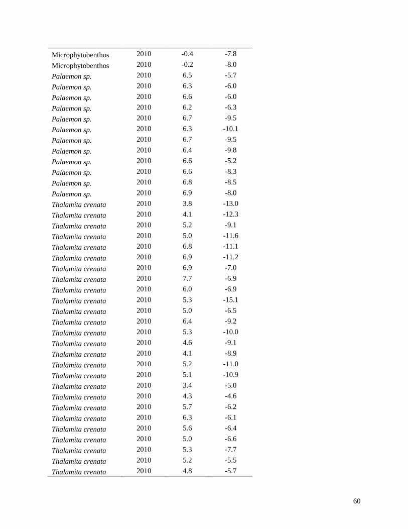
60

Microphytobenthos 2010 -0.4 -7.8

Microphytobenthos 2010 -0.2 -8.0

Palaemon sp. 2010 6.5 -5.7

Palaemon sp. 2010 6.3 -6.0

Palaemon sp. 2010 6.6 -6.0

Palaemon sp. 2010 6.2 -6.3

Palaemon sp. 2010 6.7 -9.5

Palaemon sp. 2010 6.3 -10.1

Palaemon sp. 2010 6.7 -9.5

Palaemon sp. 2010 6.4 -9.8

Palaemon sp. 2010 6.6 -5.2

Palaemon sp. 2010 6.6 -8.3

Palaemon sp. 2010 6.8 -8.5

Palaemon sp. 2010 6.9 -8.0

Thalamita crenata 2010 3.8 -13.0

Thalamita crenata 2010 4.1 -12.3

Thalamita crenata 2010 5.2 -9.1

Thalamita crenata 2010 5.0 -11.6

Thalamita crenata 2010 6.8 -11.1

Thalamita crenata 2010 6.9 -11.2

Thalamita crenata 2010 6.9 -7.0

Thalamita crenata 2010 7.7 -6.9

Thalamita crenata 2010 6.0 -6.9

Thalamita crenata 2010 5.3 -15.1

Thalamita crenata 2010 5.0 -6.5

Thalamita crenata 2010 6.4 -9.2

Thalamita crenata 2010 5.3 -10.0

Thalamita crenata 2010 4.6 -9.1

Thalamita crenata 2010 4.1 -8.9

Thalamita crenata 2010 5.2 -11.0

Thalamita crenata 2010 5.1 -10.9

Thalamita crenata 2010 3.4 -5.0

Thalamita crenata 2010 4.3 -4.6

Thalamita crenata 2010 5.7 -6.2

Thalamita crenata 2010 6.3 -6.1

Thalamita crenata 2010 5.6 -6.4

Thalamita crenata 2010 5.0 -6.6

Thalamita crenata 2010 5.3 -7.7

Thalamita crenata 2010 5.2 -5.5

Thalamita crenata 2010 4.8 -5.7

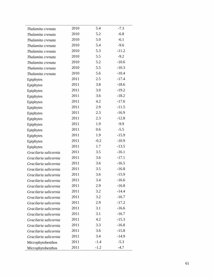
61

Thalamita crenata 2010 5.4 -7.3

Thalamita crenata 2010 5.2 -6.8

Thalamita crenata 2010 5.0 -6.1

Thalamita crenata 2010 5.4 -9.6

Thalamita crenata 2010 5.3 -11.2

Thalamita crenata 2010 5.5 -9.2

Thalamita crenata 2010 5.2 -10.6

Thalamita crenata 2010 5.5 -10.3

Thalamita crenata 2010 5.6 -10.4

Epiphytes 2011 2.5 -17.4

Epiphytes 2011 3.8 -18.6

Epiphytes 2011 3.0 -19.2

Epiphytes 2011 3.6 -18.2

Epiphytes 2011 4.2 -17.6

Epiphytes 2011 2.9 -11.5

Epiphytes 2011 2.3 -16.9

Epiphytes 2011 2.3 -12.8

Epiphytes 2011 1.9 -9.9

Epiphytes 2011 0.6 -5.5

Epiphytes 2011 1.9 -15.9

Epiphytes 2011 -0.2 -10.9

Epiphytes 2011 1.7 -13.5

Gracilaria salicornia 2011 3.5 -16.1

Gracilaria salicornia 2011 3.6 -17.1

Gracilaria salicornia 2011 3.6 -16.5

Gracilaria salicornia 2011 3.5 -16.8

Gracilaria salicornia 2011 3.6 -15.9

Gracilaria salicornia 2011 3.4 -16.6

Gracilaria salicornia 2011 2.9 -16.8

Gracilaria salicornia 2011 3.2 -14.4

Gracilaria salicornia 2011 3.2 -16.7

Gracilaria salicornia 2011 2.9 -17.2

Gracilaria salicornia 2011 3.1 -16.6

Gracilaria salicornia 2011 3.1 -16.7

Gracilaria salicornia 2011 4.2 -15.3

Gracilaria salicornia 2011 3.3 -16.8

Gracilaria salicornia 2011 3.6 -15.8

Gracilaria salicornia 2011 3.4 -14.9

Microphytobenthos 2011 -1.4 -5.3

Microphytobenthos 2011 -1.2 -4.7

62

Microphytobenthos 2011 -0.1 -4.8

Microphytobenthos 2011 -0.6 -4.7

Microphytobenthos 2011 1.1 -5.0

Microphytobenthos 2011 0.1 -6.1

Microphytobenthos 2011 -0.6 -4.9

Palaemon sp. 2011 7.5 -11.0

Palaemon sp. 2011 7.3 -11.5

Palaemon sp. 2011 6.0 -9.4

Palaemon sp. 2011 7.3 -10.7

Palaemon sp. 2011 7.1 -13.8

Palaemon sp. 2011 6.9 -13.2

Palaemon sp. 2011 7.1 -13.8

Palaemon sp. 2011 6.9 -13.6

Palaemon sp. 2011 6.9 -11.1

Palaemon sp. 2011 6.2 -10.0

Palaemon sp. 2011 6.0 -9.9

Palaemon sp. 2011 7.3 -11.3

Palaemon sp. 2011 6.2 -9.5

Phytoplankton 2011 3.2 -20.7

Phytoplankton 2011 2.8 -19.8

Phytoplankton 2011 3.0 -20.5

Phytoplankton 2011 3.1 -18.7

Phytoplankton 2011 3.5 -20.5

Phytoplankton 2011 3.2 -20.3

Phytoplankton 2011 3.3 -21.4

Phytoplankton 2011 3.5 -20.8

Phytoplankton 2011 2.8 -16.2

Phytoplankton 2011 3.0 -15.6

Phytoplankton 2011 2.0 -15.7

Phytoplankton 2011 2.1 -15.8

Phytoplankton 2011 4.0 -20.3

Phytoplankton 2011 2.1 -21.0

Phytoplankton 2011 3.0 -21.1

Phytoplankton 2011 1.9 -21.2

Thalamita crenata 2011 5.8 -11.9

Thalamita crenata 2011 6.2 -11.5

Thalamita crenata 2011 7.2 -12.2

Thalamita crenata 2011 6.0 -12.1

Thalamita crenata 2011 6.1 -12.7

Thalamita crenata 2011 6.3 -13.5

63

Thalamita crenata 2011 6.0 -11.2

Thalamita crenata 2011 5.4 -14.1

Thalamita crenata 2011 5.5 -8.3

Thalamita crenata 2011 5.7 -7.5

Thalamita crenata 2011 4.5 -5.9

Thalamita crenata 2011 4.2 -5.1

Thalamita crenata 2011 4.6 -10.7

Thalamita crenata 2011 4.1 -6.5

Thalamita crenata 2011 4.5 -8.7

Thalamita crenata 2011 4.7 -8.1

Sphyraena barracuda 2017 9.3 -12.7

Sphyraena barracuda 2017 9.6 -12.9

Sphyraena barracuda 2017 9.1 -12.2

Sphyraena barracuda 2017 10.8 -13.5

Sphyraena barracuda 2017 10.5 -13.8

Sphyraena barracuda 2017 10.1 -13.9

Sphyraena barracuda 2017 9.6 -13.6

Sphyraena barracuda 2017 9.5 -13.5

Sphyraena barracuda 2017 9.9 -13.1

Sphyraena barracuda 2017 9.0 -15.5

Sphyraena barracuda 2017 9.6 -12.9

Sphyraena barracuda 2017 9.7 -13.5

Sphyraena barracuda 2017 8.3 -14.3

Sphyraena barracuda 2017 10.1 -13.2

Osteomugil engeli 2017 5.3 -16.4

Sphyraena barracuda 2017 9.9 -13.0

Sphyraena barracuda 2017 10.8 -13.8

Sphyraena barracuda 2017 10.5 -14.3

Sphyraena barracuda 2017 10.5 -15.4

Sphyraena barracuda 2017 8.6 -14.3

Sphyraena barracuda 2017 9.6 -13.7

Sphyraena barracuda 2017 9.7 -13.6

Sphyraena barracuda 2017 10.6 -13.9

Caranx melampygus 2017 11.0 -13.0

Sphyraena barracuda 2017 10.4 -13.9

Sphyraena barracuda 2017 10.5 -14.5

Sphyraena barracuda 2017 9.8 -14.3

Sphyraena barracuda 2017 9.9 -14.3

Sphyraena barracuda 2017 10.4 -13.5

Sphyraena barracuda 2017 10.1 -15.4

64

Sphyraena barracuda 2017 10.6 -14.0

Sphyraena barracuda 2017 9.0 -12.7

Sphyraena barracuda 2017 10.7 -14.4

Sphyraena barracuda 2017 10.5 -13.3

Sphyraena barracuda 2017 8.4 -12.8

Sphyraena barracuda 2017 9.9 -13.6

Sphyraena barracuda 2017 10.9 -13.6

Sphyraena barracuda 2017 10.6 -13.9

Sphyraena barracuda 2017 10.0 -14.0

Sphyraena barracuda 2017 9.9 -13.8

Sphyraena barracuda 2017 9.9 -13.3

Caranx ignobilis 2017 10.1 -13.4

Caranx ignobilis 2017 9.7 -12.2

Sphyraena barracuda 2017 9.5 -14.7

Caranx ignobilis 2017 9.7 -11.6

Sphyraena barracuda 2017 9.6 -13.8

Sphyraena barracuda 2017 8.2 -13.5

Caranx ignobilis 2017 10.1 -14.9

Sphyraena barracuda 2017 10.3 -15.4

Sphyraena barracuda 2017 8.3 -14.1

Sphyraena barracuda 2017 9.4 -12.8

Sphyraena barracuda 2017 9.5 -12.8

Sphyraena barracuda 2017 8.1 -12.9

Caranx ignobilis 2017 9.5 -12.1

Sphyraena barracuda 2017 9.9 -12.6

Caranx melampygus 2017 9.9 -11.7

Caranx melampygus 2017 10.1 -11.6

Sphyraena barracuda 2017 10.9 -14.4

Sphyraena barracuda 2017 7.5 -12.0

Sphyraena barracuda 2017 7.5 -11.9

Caranx ignobilis 2017 8.6 -11.4

Sphyraena barracuda 2017 8.8 -14.5

Sphyraena barracuda 2017 9.3 -14.5

Sphyraena barracuda 2017 9.3 -14.5

Caranx ignobilis 2017 8.4 -11.8

Caranx ignobilis 2017 8.9 -12.7

Sphyraena barracuda 2017 9.2 -13.7

Caranx ignobilis 2017 8.1 -13.5

Sphyraena barracuda 2017 9.2 -12.9

Sphyraena barracuda 2017 9.1 -13.2

65

Sphyraena barracuda 2017 8.8 -13.5

Sphyraena barracuda 2017 8.7 -12.1

Osteomugil engeli 2017 6.4 -17.2

Osteomugil engeli 2017 6.3 -16.4

Osteomugil engeli 2017 6.3 -15.5

Osteomugil engeli 2017 6.3 -15.5

Osteomugil engeli 2017 5.8 -16.2

Osteomugil engeli 2017 6.1 -15.6

Osteomugil engeli 2017 6.2 -16.1

Osteomugil engeli 2017 6.3 -15.9

Osteomugil engeli 2017 6.1 -14.9

Osteomugil engeli 2017 5.5 -13.7

Osteomugil engeli 2017 6.0 -15.0

Osteomugil engeli 2017 7.8 -15.8

Osteomugil engeli 2017 6.4 -14.8

Osteomugil engeli 2017 6.9 -14.9

Osteomugil engeli 2017 6.5 -14.3

Osteomugil engeli 2017 6.2 -14.8

Osteomugil engeli 2017 6.4 -15.0

Osteomugil engeli 2017 6.8 -14.5

Thalamita crenata 2017 6.7 -16.9

Kuhlia sp. 2017 8.8 -16.6

Kuhlia sp. 2017 9.0 -17.5

Kuhlia sp. 2017 8.9 -15.9

Kuhlia sp. 2017 9.2 -16.3

Kuhlia sp. 2017 9.1 -17.2

Gambusia affinis 2017 5.9 -16.5

Gambusia affinis 2017 5.9 -18.6

Gambusia affinis 2017 6.0 -15.3

Gambusia affinis 2017 6.9 -15.7

Gambusia affinis 2017 5.3 -15.3

Gambusia affinis 2017 6.0 -15.8

Gambusia affinis 2017 5.8 -15.5

Gambusia affinis 2017 6.3 -15.7

Mugil cephalus 2017 5.6 -14.2

Mugil cephalus 2017 5.5 -14.2

Mugil cephalus 2017 5.5 -13.8

Mugil cephalus 2017 5.5 -13.8

Mugil cephalus 2017 5.9 -14.5

Mugil cephalus 2017 5.6 -13.2

66

Mugil cephalus 2017 5.5 -14.3

Palaemon sp. 2017 6.5 -14.1

Palaemon sp. 2017 6.7 -14.8

Palaemon sp. 2017 6.2 -14.6

Palaemon sp. 2017 6.5 -14.2

Tilapia 2017 8.1 -16.8

Tilapia 2017 8.2 -17.4

Tilapia 2017 8.2 -17.4

Tilapia 2017 8.1 -16.7

67

Table A2. Sequence identifications, length, and percent similarities from the BOLD and GenBank (with ACCN) databases.

Species identification

(BOLD)

% similarity

(BOLD)

Species identification

(GenBank)

% similarity

(GenBank)

ACCN

(GenBank)

Sequence

length

Saurida nebulosa 99.46 Halichoeres biocellatus 85 KU944629 591

Oxyurichthys lonchotus 99.28 Oxyurichthys petersi 87.6 KY176548 588

Oxyurichthys lonchotus 99.35 Oxyurichthys petersi 88.4 KY176548 630

Oxyurichthys lonchotus 99.47 Oxyurichthys petersi 88.7 KY176548 585

Oxyurichthys lonchotus 99.47 Oxyurichthys petersi 88.7 KY176548 586

Oxyurichthys lonchotus 99.47 Oxyurichthys petersi 88.7 KY176548 589

Oxyurichthys lonchotus 99.47 Oxyurichthys petersi 88.7 KY176548 587

Oxyurichthys lonchotus 99.47 Oxyurichthys petersi 88.7 KY176548 587

Oxyurichthys lonchotus 99.47 Oxyurichthys petersi 88.7 KY176548 588

Oxyurichthys lonchotus 99.47 Oxyurichthys petersi 88.7 KY176548 588

Oxyurichthys lonchotus 99.47 Oxyurichthys petersi 88.7 KY176548 575

Oxyurichthys lonchotus 99.47 Oxyurichthys petersi 88.7 KY176548 579

Oxyurichthys lonchotus 99.47 Oxyurichthys petersi 88.7 KY176548 586

Oxyurichthys lonchotus 99.29 Oxyurichthys petersi 88.8 KY176548 587

Oxyurichthys lonchotus 99.64 Oxyurichthys petersi 88.9 KY176548 588

Oxyurichthys lonchotus 99.35 Oxyurichthys petersi 89.1 KY176548 631

Oxyurichthys lonchotus 99.35 Oxyurichthys petersi 89.1 KY176548 631

Oxyurichthys lonchotus 99.47 Oxyurichthys petersi 89.1 KY176548 575

Psilogobius mainlandi 99.07 Gobiidae sp. 92.3 MG816687 554

Psilogobius mainlandi 100 Gobiidae sp. 93.3 KY675582 587

68

No match Mulloidichthys flavolineatus 97 KU944161 589

Osteomugil engeli 99.32 Osteomugil engeli 98.4 MG816711 448

Psilogobius mainlandi 99.42 Psilogobius mainlandi 98.7 MG816721 520

Mulloidichthys flavolineatus 100 Mulloidichthys flavolineatus 99.2 KY371760 543

Asterropteryx semipunctata 100 Asterropteryx semipunctata 99.2 KR059871 633

Caranx sexfasciatus 100 Caranx sexfasciatus 99.2 HQ560966 643

Thalamita crenata 99.46 Thalamita crenata 99.2 JX398104 570

Asterropteryx semipunctata 99.83 Asterropteryx semipunctata 99.3 KR059871 589

Asterropteryx semipunctata 100 Asterropteryx semipunctata 99.4 KR059871 630

Asterropteryx semipunctata 100 Asterropteryx semipunctata 99.4 KR059871 631

Psilogobius mainlandi 99.81 Psilogobius mainlandi 99.4 MG816721 556

Thalamita crenata 99.83 Thalamita crenata 99.4 JX398104 587

Foa brachygramma 99.52 Foa brachygramma 99.5 MG816687 631

Caranx ignobilis 100 Caranx ignobilis 99.5 KF649842 623

Foa brachygramma 99.51 Foa brachygramma 99.5 MG816687 632

No match Osteomugil engeli 99.6 JQ431913 590

Caranx melampygus 100 Caranx melampygus 99.6 KY371310 480

Thalamita crenata 99.81 Thalamita crenata 99.6 KT365763 538

Caranx ignobilis 100 Caranx ignobilis 99.7 FJ347936 635

Asterropteryx semipunctata 100 Asterropteryx semipunctata 99.8 KR059871 630

Albula glossodonta 99.84 Albula glossodonta 99.8 JQ431400 631

Asterropteryx semipunctata 100 Asterropteryx semipunctata 99.8 KR059871 578

Osteomugil engeli 99.82 Osteomugil engeli 99.8 JQ060502 574

Asterropteryx semipunctata 100 Asterropteryx semipunctata 99.8 KR059871 632

69

Asterropteryx semipunctata 100 Asterropteryx semipunctata 99.8 KR059871 630

Foa brachygramma 99.84 Foa brachygramma 99.8 KJ967855 634

Caranx ignobilis 100 Caranx ignobilis 99.8 KU943739 588

Foa brachygramma 99.84 Foa brachygramma 99.8 MG816687 636

Thalamita crenata 100 Thalamita crenata 99.8 JX398104 589

Atherinomorus insularum 100 Atherinomorus insularum 100 MG816654 633

Sardinella marquesensis 100 Sardinella marquesensis 100 MG816723 587

Asterropteryx semipunctata 100 Asterropteryx semipunctata 100 KR059872 577

Asterropteryx semipunctata 100 Asterropteryx semipunctata 100 KR059872 581

Thalamita crenata 99.66 Thalamita crenata 100 KT365763 599

Thalamita crenata 100 Thalamita crenata 100 JX398104 583

70

Table A3. Fork length (mm), total length (mm), weight (g), and stomach fullness (g) of all fish utilized for diet analyses.

Capture

date

Capture

time

Predator

ID Tag 1 Tag 2 Species

Fork

length

(mm)

Total

length

(mm)

Weight

(g)

Stomach

mass - full

(g)

Stomach

mass -

empty (g)

Fullness

coefficient

7/29/17 15:30 LD01

Caranx melampygus 349 415 920 17.91 8.88 3

7/29/17 17:50 LD02

Sphyraena barracuda 332 371 263.14 1.69 1.19 1

7/29/17 9:10 DA06

Sphyraena barracuda 296 346 204.8 12.72 1.05 3

7/29/17 9:15 DA07

Sphyraena barracuda 272 308 162.25 18.66 1.21 3

7/29/17 8:15 AA01

Sphyraena barracuda 355 396 299.66 4.74 1.67 2

7/29/17 8:25 DA01

Sphyraena barracuda 327 369 240.95 2.55 1.83 1

7/29/17 10:00 DA12

Sphyraena barracuda 320 282 166.5 1.25 0.93 1

7/29/17 10:40 DA15

Sphyraena barracuda 298 333 204.92 8.99 1.31 3

7/29/17 9:43 DA09

Sphyraena barracuda 280 321 166.35 1.24 0.95 1

8/11/17 2:30 KB01

Caranx ignobilis 401 480 1520 25.33 20.65 2

7/29/17 15:22 AA04

Sphyraena barracuda 507 554 800 5.14 3.98 2

7/29/17 16:07 AA18

Sphyraena barracuda 379 434 347.86 2.57 1.81 2

7/29/17 16:18 AA09

Sphyraena barracuda 350 403 343.85 4.41 2.16 2

7/29/17 16:24 AA11

Sphyraena barracuda 330 383 269.37 2.10 1.57 2

7/29/17 16:21 AA10

Sphyraena barracuda 308 350 198.38 1.33 1.08 1

7/29/17 8:20 LT01

Sphyraena barracuda 292 331 184.2 1.28 0.92 1

7/29/17 16:37 AA13

Sphyraena barracuda 318 365 258.01 1.73 1.33 1

7/29/17 16:39 AA14

Sphyraena barracuda 345 389 289.63 9.11 1.70 1

7/29/17 10:30 AA03

Sphyraena barracuda 352 394 313.18 1.72 1.24 1

7/29/17 9:40 LT02

Sphyraena barracuda 135 162 49.49 0.62 0.45 2

7/29/17 10:25 DA13

Sphyraena barracuda 282 321 182.39 2.81 1.31 2

7/29/17 15:46 AA06

Sphyraena barracuda 421 462 466.04 3.10 2.45 2

71

7/29/17 8:53 DA03

Sphyraena barracuda 317 361 221.11 6.63 2.03 3

7/29/17 9:48 DA10

Sphyraena barracuda 326 362 241.6 7.43 1.83 3

7/29/17 9:23 DA08

Sphyraena barracuda 343 380 268.16 14.24 2.37 2

7/29/17 9:05 DA05

Sphyraena barracuda 261 302 139.43 8.10 0.89 2

7/29/17 15:53 AA07

Sphyraena barracuda 438 514 536.22 10.95 3.49 1

7/29/17 15:29 AA05

Sphyraena barracuda 380 441 413.59 4.19 2.61 2

7/29/17 8:12 LM03

Sphyraena barracuda 302 337 212.27 5.32 1.53 3

7/29/17 8:52 LM06

Caranx ignobilis 243 284 286.96 6.76 2.56 3

7/29/17 10:24 LM08

Caranx ignobilis 162 196 102.33 2.33 0.98 3

7/29/17 16:12 KK05

Caranx ignobilis 212 250 206.88 2.43 2.35 2

7/29/17 10:43 LM09

Sphyraena barracuda 300 348 198.05 3.37 1.47 2

7/29/17 7:56 LM01

Sphyraena barracuda 301 344 228.14 1.46 1.24 1

7/29/17 8:30 LM05

Caranx ignobilis 252 311 414.82 4.89 4.41 2

7/29/17 8:18 LM04

Sphyraena barracuda 305 345 225.39 1.53 1.19 1

7/29/17 16:20 KK06

Sphyraena barracuda 213 252 218.48 2.86 2.00 2

7/29/17 16:54 KK09

Sphyraena barracuda 334 375 283.02 3.77 1.61 2

7/29/17 16:28 KK07

Sphyraena barracuda 316 354 239.92 2.82 1.59 2

7/29/17 15:10 KK01

Sphyraena barracuda 295 341 185.53 1.94 1.35 2

7/29/17 16:08 KK04

Sphyraena barracuda 384 428 433.26 5.73 2.40 3

7/29/17

NT01

Sphyraena barracuda 346 394 280.58 2.15 1.76 2

7/29/17 16:04 KK03 A7142 A7143 Sphyraena barracuda 332 374 263.6 5.23 1.85 3

7/29/17 18:37 KK08

Sphyraena barracuda 307 348 231.27 1.38 1.11 1

7/29/17 9:50 LM07

Sphyraena barracuda 369 406 373.63 8.68 2.92 3

7/29/17 8:05 LM02

Caranx ignobilis 275 332 473.34 5.83 4.79 2

7/29/17 16:10 AA08

Sphyraena barracuda 440 489 560.5 22.23 4.71 1

7/29/17 17:28 ER02

Sphyraena barracuda 431 484 552.44 32.86 4.49 3

7/29/17 17:07 AA15

Sphyraena barracuda 386 457 458.22 28.36 3.33 3

72

7/29/17 16:26 AA12

Sphyraena barracuda 364 407 350.83 4.43 3.00 2

7/29/17 16:01 ER01

Sphyraena barracuda 355 399 328.58 1.99 1.77 1

7/29/17 9:27 AA02

Sphyraena barracuda 325 380 284.55 4.05 1.84 2

7/29/17 10:03 DA11

Sphyraena barracuda 296 337 187.88 4.66 1.78 3

7/29/17 10:30 DA14

Sphyraena barracuda 330 371 244.34 8.33 1.71 3

7/29/17 9:00 DA04

Sphyraena barracuda 311 351 219.38 13.79 1.75 2

7/29/17 19:00 ER04

Caranx ignobilis 405 481 1580 43.70 26.82 3

7/29/17 16:59 KK10

Caranx ignobilis 275 335 451.58 7.59 7.35 2

7/29/17 15:12 KK02

Caranx ignobilis 395 477 1460 23.01 22.86 1

9/30/17

KP01

Sphyraena barracuda 353 391 280.89 2.50 1.93 2

7/29/17 18:06 AA16

Sphyraena barracuda 330 383 266.33 1.99 1.57 2

7/29/17 8:50 DA02

Caranx melampygus 335 392 820 17.99 8.69 3

7/29/17 18:31 AA17

Sphyraena barracuda 339 375 259.8 3.05 1.73 2

7/29/17 19:05 ER03

Sphyraena barracuda 389 435 379.32 3.48 2.67 2

7/29/17 16:30 AA20 A7128 A7129 Sphyraena barracuda 443 486 491.13 7.85 4.23 2

7/29/17 16:05 AA19

Sphyraena barracuda 398 451 441.27 4.67 3.99 2

12/18/17

KB02

Caranx ignobilis 433 518 1780 51.51 25.78 3

12/18/17

KB03

Caranx ignobilis 333 396 840 20.94 13.16 3

12/18/17

KB04

Caranx ignobilis 389 466 1220 28.84 19.36 2

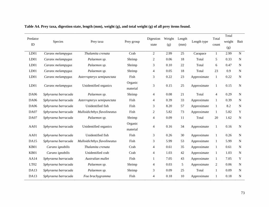
73

Table A4. Prey taxa, digestion state, length (mm), weight (g), and total weight (g) of all prey items found.

Predator

ID Species Prey taxa Prey group

Digestion

state

Weight

(g)

Length

(mm) Length type

Total

count

Total

weight

(g)

Bait

LD01 Caranx melampygus Thalamita crenata Crab 2 2.99 25 Carapace 1 2.99 N

LD01 Caranx melampygus Palaemon sp. Shrimp 2 0.06 18 Total 5 0.33 N

LD01 Caranx melampygus Palaemon sp. Shrimp 3 0.10 22 Total 6 0.47 N

LD01 Caranx melampygus Palaemon sp. Shrimp 4 0.05 18 Total 23 0.9 N

LD01 Caranx melampygus Asterropteryx semipunctata Fish 3 0.22 23 Approximate 1 0.22 N

LD01 Caranx melampygus Unidentified organics Organic

material 3 0.15 25 Approximate 1 0.15 N

DA06 Sphyraena barracuda Palaemon sp. Shrimp 4 0.08 21 Total 4 0.29 N

DA06 Sphyraena barracuda Asterropteryx semipunctata Fish 4 0.39 33 Approximate 1 0.39 N

DA06 Sphyraena barracuda Unidentified fish Fish 3 8.20 57 Approximate 1 8.2 N

DA07 Sphyraena barracuda Mulloidichthys flavolineatus Fish 2 5.82 73 Approximate 1 5.82 Y

DA07 Sphyraena barracuda Palaemon sp. Shrimp 4 0.09 11 Total 20 1.62 N

AA01 Sphyraena barracuda Unidentified organics Organic

material 4 0.16 34 Approximate 1 0.16 N

AA01 Sphyraena barracuda Unidentified fish Fish 3 0.26 30 Approximate 1 0.26 N

DA15 Sphyraena barracuda Mulloidichthys flavolineatus Fish 3 5.99 53 Approximate 1 5.99 N

KB01 Caranx ignobilis Thalamita crenata Crab 4 0.61 35 Approximate 1 0.61 N

KB01 Caranx ignobilis Unidentified crab Crab 4 1.03 42 Approximate 1 1.03 N

AA14 Sphyraena barracuda Australian mullet Fish 1 7.05 43 Approximate 1 7.05 Y

LT02 Sphyraena barracuda Palaemon sp. Shrimp 4 0.03 5 Approximate 2 0.06 N

DA13 Sphyraena barracuda Palaemon sp. Shrimp 3 0.09 25 Total 1 0.09 N

DA13 Sphyraena barracuda Foa brachygramma Fish 4 0.18 10 Approximate 1 0.18 N

74

DA13 Sphyraena barracuda Foa brachygramma Fish 4 0.08 16 Approximate 1 0.08 N

DA03 Sphyraena barracuda Unidentified fish Fish 2 0.55 29 Approximate 1 0.55 N

DA03 Sphyraena barracuda Oxyurichthys lonchotus Fish 2 0.56 28 Approximate 1 0.56 N

DA03 Sphyraena barracuda Oxyurichthys lonchotus Fish 3 0.15 17 Approximate 1 0.15 N

DA03 Sphyraena barracuda Asterropteryx semipunctata Fish 3 0.08 13 Approximate 1 0.08 N

DA03 Sphyraena barracuda Asterropteryx semipunctata Fish 3 0.07 12 Approximate 1 0.07 N

DA03 Sphyraena barracuda Asterropteryx semipunctata Fish 4 0.03 9 Approximate 1 0.03 N

DA03 Sphyraena barracuda Palaemon sp. Shrimp 2 0.13 20 Total 8 0.77 N

DA03 Sphyraena barracuda Palaemon sp. Shrimp 3 0.05 18 Approximate 6 0.29 N

DA10 Sphyraena barracuda Sardinella marquesensis Fish 2 4.18 59 Approximate 1 4.18 N

DA08 Sphyraena barracuda Unidentified fish Fish 2 1.13 41 Total 1 1.13 N

DA08 Sphyraena barracuda Psilogobius mainlandi Fish 2 0.33 34 Total 1 0.33 N

DA08 Sphyraena barracuda Psilogobius mainlandi Fish 2 0.16 22 Total 1 0.16 N

DA08 Sphyraena barracuda Palaemon sp. Shrimp 1 0.21 22 Total 1 0.21 N

DA08 Sphyraena barracuda Palaemon sp. Shrimp 2 0.03 16 Total 33 2.91 N

DA05 Sphyraena barracuda Foa brachygramma Fish 2 1.38 25 Approximate 1 1.38 N

DA05 Sphyraena barracuda Foa brachygramma Fish 3 0.78 28 Approximate 1 0.78 N

AA07 Sphyraena barracuda Australian mullet Fish 1 6.68 73 Approximate 1 6.68 Y

LM03 Sphyraena barracuda Oxyurichthys lonchotus Fish 2 2.20 70 Total 1 2.20 N

LM03 Sphyraena barracuda Oxyurichthys lonchotus Fish 4 0.21 23 Approximate 1 0.21 N

LM03 Sphyraena barracuda Oxyurichthys lonchotus Fish 4 0.07 11 Approximate 1 0.07 N

LM06 Caranx ignobilis Unidentified fish Fish 3 0.41 35 Standard 1 0.41 N

LM06 Caranx ignobilis Unidentified fish Fish 2 1.89 75 Total 1 1.89 N

LM06 Caranx ignobilis Unidentified fish Fish 3 0.45 42 Standard 1 0.45 N

LM06 Caranx ignobilis Caranx melampygus Fish 4 0.05 15 Approximate 1 0.05 N

LM06 Caranx ignobilis Palaemon sp. Shrimp 2 0.08 21 Total 1 0.08 N

LM06 Caranx ignobilis Palaemon sp. Shrimp 2 0.08 21 Total 1 0.08 N

75

LM06 Caranx ignobilis Palaemon sp. Shrimp 2 0.09 20 Total 1 0.09 N

LM06 Caranx ignobilis Palaemon sp. Shrimp 3 0.04 16 Total 1 0.04 N

LM06 Caranx ignobilis Palaemon sp. Shrimp 3 0.08 22 Total 1 0.08 N

LM06 Caranx ignobilis Palaemon sp. Shrimp 4 0.02 7 Approximate 1 0.02 N

LM06 Caranx ignobilis Palaemon sp. Shrimp 4 0.02 10 Approximate 1 0.02 N

LM08 Caranx ignobilis Caranx ignobilis Fish 2 1.04 47 Total 1 1.04 N

KK05 Caranx ignobilis Palaemon sp. Shrimp 4 0.01 6 Approximate 1 0.01 N

LM09 Sphyraena barracuda Otolith Fish 4 1 NA N

LM09 Sphyraena barracuda Oxyurichthys lonchotus Fish 4 0.23 40 Approximate 1 0.23 N

LM09 Sphyraena barracuda Palaemon sp. Shrimp 2 0.11 24 Total 1 0.11 N

LM09 Sphyraena barracuda Palaemon sp. Shrimp 4 0.05 16 Approximate 4 0.35 N

LM05 Caranx ignobilis Palaemon sp. Shrimp 4 0.02 7 Approximate 2 0.06 N

KK06 Sphyraena barracuda Caranx sexfasciatus Fish 4 0.03 23 Approximate 1 0.03 N

KK09 Sphyraena barracuda Algae Algae 2 0.31 67 Total 1 0.31 N

KK09 Sphyraena barracuda Oxyurichthys lonchotus Fish 4 0.03 10 Total 1 0.03 N

KK09 Sphyraena barracuda Oxyurichthys lonchotus Fish 4 0.06 15 Total 1 0.06 N

KK09 Sphyraena barracuda Oxyurichthys lonchotus Fish 4 0.01 14 Total 1 0.01 N

KK09 Sphyraena barracuda Otolith Fish 4 2 NA N

KK07 Sphyraena barracuda Unidentified fish Fish 2 0.07 12 Approximate 1 0.07 N

KK07 Sphyraena barracuda Oxyurichthys lonchotus Fish 4 0.05 18 Total 1 0.05 N

KK01 Sphyraena barracuda Palaemon sp. Shrimp 4 0.02 8 Approximate 1 0.02 N

KK01 Sphyraena barracuda Unidentified organics Organic

material 3 0.07 25 Total 1 0.07 N

KK04 Sphyraena barracuda Oxyurichthys lonchotus Fish 3 0.33 28 Approximate 1 0.33 N

KK04 Sphyraena barracuda Oxyurichthys lonchotus Fish 3 0.94 45 Approximate 1 0.94 N

KK04 Sphyraena barracuda Unidentified fish Fish 3 0.64 42 Approximate 1 0.64 N

KK04 Sphyraena barracuda Algae Algae 2 0.16 25 Total 1 0.16 N

76

KK04 Sphyraena barracuda Algae Algae 2 0.18 23 Total 1 0.18 N

NT01 Sphyraena barracuda Unidentified fish Fish 3 0.18 21 Approximate 1 0.18 N

KK03 Sphyraena barracuda Oxyurichthys lonchotus Fish 2 1.91 62 Total 1 1.91 N

KK03 Sphyraena barracuda Oxyurichthys lonchotus Fish 3 0.78 30 Approximate 1 0.78 N

KK03 Sphyraena barracuda Algae Algae 2 0.07 30 Total 1 0.07 N

KK03 Sphyraena barracuda Algae Algae 2 0.04 18 Total 1 0.04 N

LM07 Sphyraena barracuda Oxyurichthys lonchotus Fish 2 2.36 78 Total 1 2.36 N

LM07 Sphyraena barracuda Oxyurichthys lonchotus Fish 2 2.10 67 Total 1 2.10 N

LM07 Sphyraena barracuda Oxyurichthys lonchotus Fish 4 0.23 36 Approximate 1 0.23 N

LM02 Caranx ignobilis Caranx ignobilis Fish 4 0.05 10 Approximate 1 0.05 N

LM02 Caranx ignobilis Caranx ignobilis Fish 4 0.05 18 Approximate 1 0.05 N

AA08 Sphyraena barracuda Gobiid Fish 1 8.04 90 Total 1 8.04 Y

AA08 Sphyraena barracuda Gobiid Fish 1 7.98 89 Total 1 7.98 Y

ER02 Sphyraena barracuda Mulloidichthys flavolineatus Fish 1 7.88 74 Approximate 1 7.88 Y

ER02 Sphyraena barracuda Osteomugil engeli Fish 1 14.61 67 Approximate 1 14.61 N

ER02 Sphyraena barracuda Unidentified organics Organic

material 4 0.10 10 Approximate 1 0.10 N

ER02 Sphyraena barracuda Mulloidichthys flavolineatus Fish 1 0.61 40 Approximate 1 0.61 Y

AA15 Sphyraena barracuda Osteomugil engeli Fish 2 13.06 62 Approximate 1 13.06 N

AA15 Sphyraena barracuda Osteomugil engeli Fish 1 7.49 87 Total 1 7.49 N

AA15 Sphyraena barracuda Saurida nebulosa Fish 4 0.02 21 Approximate 1 0.02 N

AA12 Sphyraena barracuda Albula glossodonta Fish 4 0.81 48 Approximate 1 0.81 N

AA12 Sphyraena barracuda Unidentified organics Organic

material 4 0.23 17 Approximate 1 0.23 N

AA02 Sphyraena barracuda Atherinomorus insularum Fish 3 1.48 57 Approximate 1 1.48 N

AA02 Sphyraena barracuda Anthropogenic debris Anthropogenic

debris 0 0.21 16L x 15W 1 0.21 N

77

DA11 Sphyraena barracuda Asterropteryx semipunctata Fish 3 2.54 60 Approximate 1 2.54 N

DA14 Sphyraena barracuda Palaemon sp. Shrimp 2 0.05 19 Total 12 1.01 N

DA14 Sphyraena barracuda Palaemon sp. Shrimp 3 0.08 21 Total 35 2.65 N

DA14 Sphyraena barracuda Palaemon sp. Shrimp 4 0.04 17 Total 14 0.45 N

DA14 Sphyraena barracuda Algae Algae 1 0.17 28 Longest 5 0.17 N

DA14 Sphyraena barracuda Algae Algae 3 0.19 22 Longest 9 0.19 N

DA14 Sphyraena barracuda Asterropteryx semipunctata Fish 3 0.26 33 Total 1 0.26 N

DA04 Sphyraena barracuda Psilogobius mainlandi Fish 2 0.42 33 Total 1 0.42 N

DA04 Sphyraena barracuda Unidentified fish Fish 3 0.09 24 Total 1 0.09 N

DA04 Sphyraena barracuda Palaemon sp. Shrimp 2 0.12 21 Total 6 0.47 N

DA04 Sphyraena barracuda Palaemon sp. Shrimp 4 0.04 18 Total 1 0.04 N

DA04 Sphyraena barracuda Palaemon sp. Shrimp 4 0.01 9 Approximate 1 0.01 N

ER04 Caranx ignobilis Thalamita crenata Crab 2 2.00 21 Shell width 1 2.00 N

ER04 Caranx ignobilis Thalamita crenata Crab 3 1.16 19 Shell width 1 1.16 N

ER04 Caranx ignobilis Unidentified crab Crab 3 3.34 24 Shell width 1 3.34 N

ER04 Caranx ignobilis Unidentified crab Crab 3 1.27 21 Shell width 1 1.27 N

ER04 Caranx ignobilis Unidentified crab Crab 4 1.07 17 Shell width 1 1.07 N

ER04 Caranx ignobilis Thalamita crenata Crab 4 0.37 12 Shell width 1 2.74 N

KK10 Caranx ignobilis Palaemon sp. Shrimp 2 0.16 21 Total 1 0.16 N

DA02 Caranx melampygus Asterropteryx semipunctata Fish 1 1.19 46 Total 1 1.19 N

DA02 Caranx melampygus Asterropteryx semipunctata Fish 1 1.15 45 Total 1 1.15 N

DA02 Caranx melampygus Unidentified fish Fish 3 0.21 30 Approximate 1 0.21 N

DA02 Caranx melampygus Unidentified fish Fish 3 0.07 22 Approximate 1 0.07 N

DA02 Caranx melampygus Asterropteryx semipunctata Fish 3 0.14 17 Approximate 1 0.14 N

DA02 Caranx melampygus Psilogobius mainlandi Fish 4 0.21 33 Approximate 1 0.21 N

DA02 Caranx melampygus Unidentified fish Fish 4 0.16 27 Approximate 1 0.16 N

DA02 Caranx melampygus Unidentified fish Fish 4 0.07 14 Approximate 1 0.07 N

78

DA02 Caranx melampygus Thalamita crenata Crab 1 0.97 10 Shell width 1 0.97 N

DA02 Caranx melampygus Palaemon sp. Shrimp 2 0.10 22 Total 11 0.82 N

DA02 Caranx melampygus Palaemon sp. Shrimp 3 0.28 29 Total 13 1.07 N

DA02 Caranx melampygus Palaemon sp. Shrimp 4 0.05 21 Total 7 0.37 N

AA17 Sphyraena barracuda Unidentified fish Fish 4 0.02 17 Approximate 1 0.02 N

AA17 Sphyraena barracuda Unidentified fish Fish 4 0.04 16 Approximate 1 0.04 N

ER03 Sphyraena barracuda Bivalve shell Mollusk 4 0.15 10 Total 1 0.15 N

ER03 Sphyraena barracuda Otoliths Fish 4 4 NA N

ER03 Sphyraena barracuda Anthropogenic debris Anthropogenic

debris 4 0.06 8 Total 1 0.06 N

ER03 Sphyraena barracuda Anthropogenic debris Anthropogenic

debris 4 0.08 8 Total 1 0.08 N

KB02 Caranx ignobilis Unidentified crab Crab 2 7.43 28 Carapace 1 7.43 N

KB02 Caranx ignobilis Unidentified crab Crab 3 5.42 25 Carapace 1 5.42 N

KB02 Caranx ignobilis Unidentified crab Crab 3 5.09 13 Approximate 1 5.09 N

KB02 Caranx ignobilis Unidentified crab Crab 3 3.58 13 Approximate 1 3.58 N

KB02 Caranx ignobilis Crab mush Crab 4 2.34 NA NA NA 2.34 N

KB03 Caranx ignobilis Unidentified crab Crab 3 3.80 NA NA 6 3.80 N

KB03 Caranx ignobilis Unidentified crab Crab 4 2.72 NA NA 1 2.72 N

KB03 Caranx ignobilis Crab mush Crab 4 1.00 NA NA 1 1.00 N

KB04 Caranx ignobilis Unidentified crab Crab 3 5.27 NA NA 3 5.27 N

KB04 Caranx ignobilis Unidentified crab Crab 4 3.81 NA NA 1 3.81 N