Precision Measurement of the Proton Electric to

Magnetic Form Factor Ratio with BLAST

by

Christopher Blair Crawford

Submitted to the Department of Physicsin partial fulfillment of the requirements for the degree of

Doctor of Philosophy in Physics

at the

MASSACHUSETTS INSTITUTE OF TECHNOLOGY

May 2005

c© Massachusetts Institute of Technology 2005. All rights reserved.

Author . . . . . . . . . . . . . . . . . . . . . . . . . . . . . . . . . . . . . . . . . . . . . . . . . . . . . . . . . . . . . .Department of Physics

May 19, 2005

Certified by. . . . . . . . . . . . . . . . . . . . . . . . . . . . . . . . . . . . . . . . . . . . . . . . . . . . . . . . . .Haiyan Gao

Associate Professor of PhysicsThesis Supervisor

Accepted by . . . . . . . . . . . . . . . . . . . . . . . . . . . . . . . . . . . . . . . . . . . . . . . . . . . . . . . . .Thomas J. Greytak

Chairman, Department Committee on Graduate Students

2

Precision Measurement of the Proton Electric to Magnetic

Form Factor Ratio with BLAST

by

Christopher Blair Crawford

Submitted to the Department of Physicson May 19, 2005, in partial fulfillment of the

requirements for the degree ofDoctor of Philosophy in Physics

Abstract

We have measured GpE/Gp

M at Q2 = 0.15–0.65 (GeV/c)2 in the South Hall Ring ofthe MIT-Bates Linear Accelerator Facility. This experiment used a polarized electronbeam, a pure hydrogen internal polarized target, and the symmetric Bates Large Ac-ceptance Spectrometer Toroid (BLAST) detector. By measuring the spin-dependent

elastic ~H(~e, e′p) asymmetry in both sectors simultaneously, we could extract the formfactor ratio independent of beam and target polarization. This was the first experi-ment to measure Gp

E/GpM using a polarized target, which is complementary to recoil

polarimetry experiments.

Thesis Supervisor: Haiyan GaoTitle: Associate Professor of Physics

3

4

Acknowledgments

I would like to express gratitude to my advisor, Haiyan Gao, for giving me interest-

ing, challenging problems to work on, and making sure that I had the resources to

be successful in my endeavors. She has been a strong advocate, and her optimistic

attitude has motivated me to improve. I also thank my thesis committee members,

Bob Redwine and Ernie Moniz, for their thoughtful comments and suggestions. I

acknowledge Professors Ricardo Alarcon, Bill Bertozzi, John Calarco, Haiyan Gao,

June Matthews, Richard Milner, and Bob Redwine for their vital role in the devel-

opment and guidance of the BLAST physics program. This work was supported by

a grant from the U.S. Department of Energy.

I was very privileged to work on this experiment with the exceptionally talented

and friendly staff at Bates Linear Accelerator Center and MIT including Taylan

Akdogan, Tancredi Botto, Karen Dow, Manouch Farkhondeh, Bill Franklin, Doug

Hasell, Ernie Ihloff, Jim Kelsey, Michael Kohl, Hauke Kolster, Tim Smith, Stan

Sobczynski, Chris Tschalar, Genya Tsentalovich, Bill Turichnetz, Townsend Zwart,

the accelerator operators, and radiation protection officers. They were always willing

to go out of their way to help me with problems. Their creative ideas, stimulating

conversions, and encouragement have helped to make Bates a wonderful learning

environment that I will remember with fondness. The engineers and technicians at

Bates did an outstanding job designing and building the BLAST detector, solving

problems with the experiment, and keeping it running smoothly. Thanks to Ernie

Bisson for maintaining our computers, for his immediate response and quick solutions

when anything went wrong.

I would like to acknowledge the tireless efforts of my fellow graduate students work-

ing on BLAST: Ben Clasie, Adam Degrush, Tavi Filoti, Eugene Geis, Pete Karpius,

Aaron Maschinot, Nikolas Meitanis, Jason Seely, Adrian Sindile, Yuan Xiao, Chi

Zhang, and Vitaliy Ziskin. Each person made major contributions to the experiment,

and spent countless hours on shift commissioning the detector and taking production

data. I learned a lot by working together with Chi Zhang and Tim Smith on the

5

BLAST reconstruction software and benefited from many enlightening conversations

with them.

Thanks to Vitaliy Ziskin, Aaron Maschinot, Ben Clasie, Jason Seely, Taylan Ak-

dogan, Akihisa Shinozaki, Tim Smith, Haiyan Gao, John Calarco, and Joy Gurrie for

contributing figures in this thesis, and to Karen Dow and Haiyan Gao, Michael Kohl

for the many helpful comments while reviewing it.

Thanks to Ernie Ihloff for bringing me up to speed in construction of the laser-

driven target, for helping with the many problems we faced with the target, and

for his helpful advice in general. Michael Grossman machined most of the custom

components of the target, always promptly and accommodating last minute changes.

George Sechen provided valuable assistance in the lab. Our research group, Tim

Black, Ben Clasie, Jason Seely, Dipankar Dutta, Feng Xiong, and Wang Xu made

valuable contributions to the target. Ben and Jason took over the target and made

dramatic improvements to get the high figure of merit quoted herein. Thanks, Ben

and Jason, for being such good friends, and for all you have done for me.

I feel the deepest gratitude for my wife Kimberly, for her unwavering support

and faith in me during our extended time in graduate school. She has given me the

strength and encouragement I needed to complete this work. Thanks, Curtis, Nicole,

and Elizabeth, for being understanding while I have been been away for such long

hours finishing this thesis. Curtis has inspired me by writing his own book at the

same time I was writing. I thank our parents for their encouragement and support.

This has truly been an accomplishment of our whole family, and I could not have

done it without them.

6

Contents

1 Physics Overview 17

1.1 Formalism . . . . . . . . . . . . . . . . . . . . . . . . . . . . . . . . . 20

1.1.1 Kinematics . . . . . . . . . . . . . . . . . . . . . . . . . . . . 22

1.1.2 Form Factors . . . . . . . . . . . . . . . . . . . . . . . . . . . 24

1.1.3 Dynamics . . . . . . . . . . . . . . . . . . . . . . . . . . . . . 26

1.2 Existing Data . . . . . . . . . . . . . . . . . . . . . . . . . . . . . . . 28

1.2.1 Rosenbluth Separation . . . . . . . . . . . . . . . . . . . . . . 29

1.2.2 Proton RMS Radius . . . . . . . . . . . . . . . . . . . . . . . 30

1.2.3 Higher Q2 Unpolarized Data . . . . . . . . . . . . . . . . . . . 33

1.2.4 Polarized Data . . . . . . . . . . . . . . . . . . . . . . . . . . 36

1.2.5 Global Analysis . . . . . . . . . . . . . . . . . . . . . . . . . . 38

1.2.6 Two-photon Contribution . . . . . . . . . . . . . . . . . . . . 42

1.3 Theoretical Descriptions of the Nucleon Form Factors . . . . . . . . . 47

1.3.1 Perturbative QCD . . . . . . . . . . . . . . . . . . . . . . . . 48

1.3.2 Constituent Quark Models . . . . . . . . . . . . . . . . . . . . 48

1.3.3 VMD Models . . . . . . . . . . . . . . . . . . . . . . . . . . . 51

1.3.4 Lattice QCD . . . . . . . . . . . . . . . . . . . . . . . . . . . 53

1.4 Current Experiment . . . . . . . . . . . . . . . . . . . . . . . . . . . 56

1.4.1 Experimental Overview . . . . . . . . . . . . . . . . . . . . . . 56

1.4.2 Physics Impact . . . . . . . . . . . . . . . . . . . . . . . . . . 57

2 Experimental Setup 59

2.1 Polarized Beam . . . . . . . . . . . . . . . . . . . . . . . . . . . . . . 59

7

2.1.1 Polarized Source . . . . . . . . . . . . . . . . . . . . . . . . . 59

2.1.2 Storage Ring . . . . . . . . . . . . . . . . . . . . . . . . . . . 60

2.1.3 Compton Polarimeter . . . . . . . . . . . . . . . . . . . . . . . 64

2.2 Polarized Targets . . . . . . . . . . . . . . . . . . . . . . . . . . . . . 66

2.2.1 Atomic Beam Source . . . . . . . . . . . . . . . . . . . . . . . 68

2.2.2 Laser Driven Source . . . . . . . . . . . . . . . . . . . . . . . 73

2.3 The BLAST Detector Package . . . . . . . . . . . . . . . . . . . . . . 86

2.3.1 BLAST Toroid . . . . . . . . . . . . . . . . . . . . . . . . . . 91

2.3.2 Drift Chambers . . . . . . . . . . . . . . . . . . . . . . . . . . 93

2.3.3 TOF Scintillators . . . . . . . . . . . . . . . . . . . . . . . . . 98

2.3.4 Cerenkov Detectors . . . . . . . . . . . . . . . . . . . . . . . . 102

2.4 Electronics and Software . . . . . . . . . . . . . . . . . . . . . . . . . 104

2.4.1 Trigger . . . . . . . . . . . . . . . . . . . . . . . . . . . . . . . 104

2.4.2 Data Acquisition . . . . . . . . . . . . . . . . . . . . . . . . . 106

2.4.3 Online Monitor . . . . . . . . . . . . . . . . . . . . . . . . . . 108

2.4.4 Reconstruction Library . . . . . . . . . . . . . . . . . . . . . . 109

3 Data Analysis 113

3.1 Event Selection . . . . . . . . . . . . . . . . . . . . . . . . . . . . . . 114

3.1.1 Elastic TOF Cuts . . . . . . . . . . . . . . . . . . . . . . . . . 115

3.1.2 Elastic WC Cuts . . . . . . . . . . . . . . . . . . . . . . . . . 116

3.1.3 Q2 Determination . . . . . . . . . . . . . . . . . . . . . . . . . 119

3.1.4 Yields . . . . . . . . . . . . . . . . . . . . . . . . . . . . . . . 119

3.1.5 Luminosity . . . . . . . . . . . . . . . . . . . . . . . . . . . . 121

3.2 Asymmetry . . . . . . . . . . . . . . . . . . . . . . . . . . . . . . . . 123

3.2.1 Raw Asymmetry . . . . . . . . . . . . . . . . . . . . . . . . . 125

3.2.2 Background Correction . . . . . . . . . . . . . . . . . . . . . . 128

3.2.3 Radiative Correction . . . . . . . . . . . . . . . . . . . . . . . 129

3.3 Form Factor Ratio . . . . . . . . . . . . . . . . . . . . . . . . . . . . 130

3.3.1 Single Asymmetry Extraction . . . . . . . . . . . . . . . . . . 131

8

3.3.2 Super-ratio Extraction . . . . . . . . . . . . . . . . . . . . . . 133

3.3.3 Global Fit Extraction . . . . . . . . . . . . . . . . . . . . . . . 134

3.4 Systematic Errors . . . . . . . . . . . . . . . . . . . . . . . . . . . . . 135

3.4.1 Drift Chamber Q2 Determination . . . . . . . . . . . . . . . . 136

3.4.2 TOF Q2 Determination . . . . . . . . . . . . . . . . . . . . . . 137

3.4.3 Target Spin Angle . . . . . . . . . . . . . . . . . . . . . . . . 139

3.4.4 Monte Carlo Simulation . . . . . . . . . . . . . . . . . . . . . 140

3.4.5 Binning and Cuts . . . . . . . . . . . . . . . . . . . . . . . . . 143

3.4.6 False Asymmetry . . . . . . . . . . . . . . . . . . . . . . . . . 143

3.4.7 Pion Contamination . . . . . . . . . . . . . . . . . . . . . . . 147

4 Results and Discussion 149

4.1 Form Factor Ratio . . . . . . . . . . . . . . . . . . . . . . . . . . . . 149

4.2 Individual Form Factors . . . . . . . . . . . . . . . . . . . . . . . . . 151

4.3 Discussion of Errors . . . . . . . . . . . . . . . . . . . . . . . . . . . . 156

4.4 Outlook . . . . . . . . . . . . . . . . . . . . . . . . . . . . . . . . . . 157

A Linear Calibrations 161

A.1 Least Squares Fit . . . . . . . . . . . . . . . . . . . . . . . . . . . . . 161

A.1.1 Generalizations of the Linear Fit . . . . . . . . . . . . . . . . 163

A.1.2 Minimum χ2 from a Least Squares Fit . . . . . . . . . . . . . 166

A.2 TOF Scintillator Offsets . . . . . . . . . . . . . . . . . . . . . . . . . 168

A.2.1 Cosmic Coincidences . . . . . . . . . . . . . . . . . . . . . . . 169

A.2.2 Elastic Coplanarity . . . . . . . . . . . . . . . . . . . . . . . . 172

A.3 Drift Chamber Time-to-Distance Function . . . . . . . . . . . . . . . 173

A.3.1 Garfield Simulation . . . . . . . . . . . . . . . . . . . . . . . . 173

A.3.2 Iterative Relaxation Method . . . . . . . . . . . . . . . . . . . 174

A.3.3 Least Squares Linear Calibration . . . . . . . . . . . . . . . . 175

B Cross Section Data 181

9

10

List of Figures

1-1 Diagrams of the lowest-order ep scattering amplitudes. . . . . . . . . 21

1-2 Kinematics of the polarized elastic scattering OPE amplitude. . . . . 22

1-3 The ep-helicity asymmetry for different target spin angles. . . . . . . 28

1-4 The GE and GM world unpolarized data. . . . . . . . . . . . . . . . . 31

1-5 The first measurement of the ~H(~e, e′p) asymmetry. . . . . . . . . . . 37

1-6 The µGE/GM world data on the proton. . . . . . . . . . . . . . . . . 39

1-7 Phenomenological fits to the µGE/GM world data. . . . . . . . . . . . 42

1-8 Scaling of the Dirac and Pauli form factors at large Q2. . . . . . . . . 49

1-9 Diagram of the Vector Meson Dominance (VMD) amplitude. . . . . . 51

1-10 Models of µGE/GM based on dispersion theory and VMD. . . . . . . 54

2-1 Plan of the BATES Linear Accelerator Center. . . . . . . . . . . . . . 61

2-2 Yield and asymmetry results of the Compton polarimeter. . . . . . . 64

2-3 Time-dependence of the beam polarization. . . . . . . . . . . . . . . . 65

2-4 Compton measurements in conjunction with the spin flipper. . . . . . 66

2-5 Schematic of the Bates Atomic Beam Source (ABS). . . . . . . . . . . 69

2-6 Polarization-dependent simulation of the ABS magnetic optics. . . . . 70

2-7 Hyperfine structure of hydrogen and deuterium. . . . . . . . . . . . . 71

2-8 Optical pumping cycle with an intermediary alkali species. . . . . . . 74

2-9 Optical pumping of the potassium D1 line. . . . . . . . . . . . . . . . 75

2-10 Laser-Driven Source (LDS) Schematic. . . . . . . . . . . . . . . . . . 76

2-11 LDS Components. . . . . . . . . . . . . . . . . . . . . . . . . . . . . . 80

2-12 Spin-cell, oven, and vacuum seal mount to the chamber. . . . . . . . . 81

11

2-13 Stand-alone dissociator performance. . . . . . . . . . . . . . . . . . . 82

2-14 Drawing of the complete LDS apparatus. . . . . . . . . . . . . . . . . 85

2-15 Temperature dependence of LDS dissociation. . . . . . . . . . . . . . 87

2-16 Laser wavelength scan of the potassium D1 resonance. . . . . . . . . 87

2-17 The BLAST detector package. . . . . . . . . . . . . . . . . . . . . . . 90

2-18 Magnetic field map of BLAST. . . . . . . . . . . . . . . . . . . . . . . 92

2-19 Steps of track reconstruction from hits in the drift chambers. . . . . . 96

2-20 An application of the Newton-Rhapson method to track fitting. . . . 97

2-21 Drift chamber tracking efficiency. . . . . . . . . . . . . . . . . . . . . 98

2-22 Timing vs. coplanarity for TOF paddle L9B. . . . . . . . . . . . . . . 101

2-23 TOF efficiency. . . . . . . . . . . . . . . . . . . . . . . . . . . . . . . 102

2-24 Schematic of the trigger logic. . . . . . . . . . . . . . . . . . . . . . . 105

2-25 Integration of online display (NSED) with ROOT analysis package. . 109

3-1 TOF scintillator timing and coplanarity cuts. . . . . . . . . . . . . . 116

3-2 Drift chamber offsets and cuts based on redundant track parameters. 118

3-3 Invariant mass (W ) and missing mass squared (M2X) spectra. . . . . . 119

3-4 Yield for each run normalized by charge. . . . . . . . . . . . . . . . . 120

3-5 The normalized yield in each Q2 bin. . . . . . . . . . . . . . . . . . . 121

3-6 Pressure in the UGBS as a function of time. . . . . . . . . . . . . . . 123

3-7 Comparison of the ABS yield with a Monte Carlo (MC) simulation. . 124

3-8 Raw experimental asymmetries in each sector. . . . . . . . . . . . . . 126

3-9 Comparison of three methods of extracting µGE/GM . . . . . . . . . . 130

3-10 Single-asymmetry extraction of µGE/GM . . . . . . . . . . . . . . . . 132

3-11 Extraction of the target spin angle from a fit of AL and AR. . . . . . 133

3-12 The P and β-dependence of the χ2 fit function. . . . . . . . . . . . . 136

3-13 Discrepancy in Q2 between electron and proton kinematics. . . . . . . 138

3-14 Comparison of Q2 from the TOFs and the drift chambers. . . . . . . 139

3-15 Analysis of Monte Carlo data. . . . . . . . . . . . . . . . . . . . . . . 142

3-16 Asymmetry and form factor ratio analyzed in fine bins. . . . . . . . . 144

12

3-17 Analysis of data divided into six sequential run periods. . . . . . . . . 145

3-18 Beam and target single spin asymmetries. . . . . . . . . . . . . . . . 146

3-19 Pion yields as a function of M2X and W . . . . . . . . . . . . . . . . . 147

4-1 BLAST results of µGE/GM based on Q2WC . . . . . . . . . . . . . . . 150

4-2 Rosenbluth separation of GE and GM constrained by R = GE/GM . . 153

4-3 BLAST extraction of GE and GM from the world unpolarized data. . 154

4-4 Recent results of GnE from polarization experiments. . . . . . . . . . . 155

4-5 BLAST results of µGE/GM based on TOF corrections to Q2WC . . . . 158

A-1 Robust fit by separation of slope and offset . . . . . . . . . . . . . . . 165

A-2 Timing peaks of cosmic coincidences in each paddle combination. . . 171

A-3 Widths and residuals of cosmic coincidence timing peaks. . . . . . . . 172

A-4 Garfield simulation of time-to-distance function. . . . . . . . . . . . . 174

A-5 Hyperbolic parametrization of the time-to-distance function. . . . . . 176

A-6 Stub types used in linear calibration of the T2D function. . . . . . . . 177

A-7 Fit to the vertex of a stub crossing the wire. . . . . . . . . . . . . . . 178

A-8 Test of the hyperbolic T2D functions. . . . . . . . . . . . . . . . . . . 179

13

14

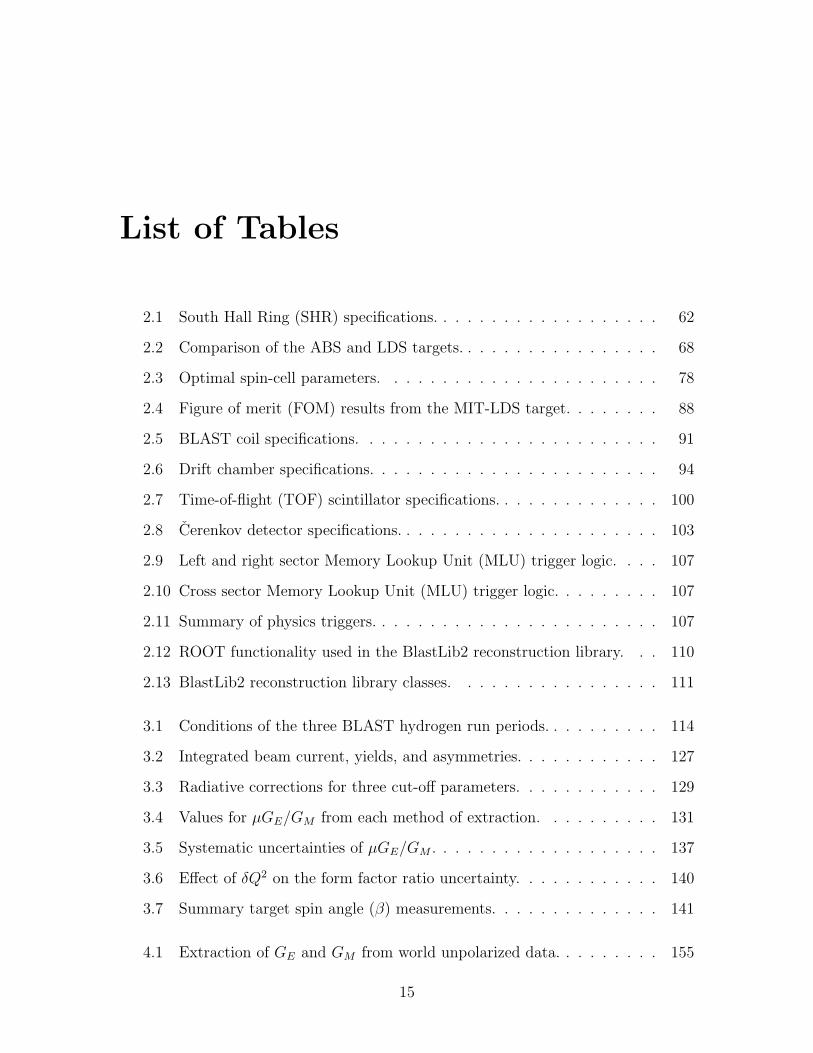
List of Tables

2.1 South Hall Ring (SHR) specifications. . . . . . . . . . . . . . . . . . . 62

2.2 Comparison of the ABS and LDS targets. . . . . . . . . . . . . . . . . 68

2.3 Optimal spin-cell parameters. . . . . . . . . . . . . . . . . . . . . . . 78

2.4 Figure of merit (FOM) results from the MIT-LDS target. . . . . . . . 88

2.5 BLAST coil specifications. . . . . . . . . . . . . . . . . . . . . . . . . 91

2.6 Drift chamber specifications. . . . . . . . . . . . . . . . . . . . . . . . 94

2.7 Time-of-flight (TOF) scintillator specifications. . . . . . . . . . . . . . 100

2.8 Cerenkov detector specifications. . . . . . . . . . . . . . . . . . . . . . 103

2.9 Left and right sector Memory Lookup Unit (MLU) trigger logic. . . . 107

2.10 Cross sector Memory Lookup Unit (MLU) trigger logic. . . . . . . . . 107

2.11 Summary of physics triggers. . . . . . . . . . . . . . . . . . . . . . . . 107

2.12 ROOT functionality used in the BlastLib2 reconstruction library. . . 110

2.13 BlastLib2 reconstruction library classes. . . . . . . . . . . . . . . . . 111

3.1 Conditions of the three BLAST hydrogen run periods. . . . . . . . . . 114

3.2 Integrated beam current, yields, and asymmetries. . . . . . . . . . . . 127

3.3 Radiative corrections for three cut-off parameters. . . . . . . . . . . . 129

3.4 Values for µGE/GM from each method of extraction. . . . . . . . . . 131

3.5 Systematic uncertainties of µGE/GM . . . . . . . . . . . . . . . . . . . 137

3.6 Effect of δQ2 on the form factor ratio uncertainty. . . . . . . . . . . . 140

3.7 Summary target spin angle (β) measurements. . . . . . . . . . . . . . 141

4.1 Extraction of GE and GM from world unpolarized data. . . . . . . . . 155

15

A.1 Statistical measures of central tendency. . . . . . . . . . . . . . . . . 164

B.1 World data used for the extraction of GE and GM . . . . . . . . . . . 181

16

Chapter 1

Physics Overview

Although the atomic constituents, the electron and nucleons, are all spin 12

particles

of charge −e, +e, and 0, they are fundamentally different. In the standard model,

the electron is a point Dirac particle which interacts electromagnetically by exchang-

ing virtual photons, as described by Quantum Electrodynamics (QED). The weak

coupling to the photon, α ≈ 1/137, guarantees that interaction amplitudes can be

calculated perturbatively. As a result, QED is very well understood and has been

tested to 3 ppb [1] in experiments like the hydrogen Lamb shift.

In contrast, the proton is 1836 times more massive than the electron and has

internal structure, first observed through its anomalous magnetic moment. In a sim-

plistic picture, it is composed of three bound valence quarks which interact through

Quantum Chromodynamics (QCD) by the exchange of virtual gluons. Unlike QED,

the coupling to gluons αS ≈ 1 is strong and increases as the energy decreases. In fact,

the gluons interact among themselves further enhancing the nonperturbative nature

of QCD. Quarks and gluons cannot exist in isolation, but only in bound states as

mesons and baryons, a property known as confinement.

Due to confinement, the proton and neutron are the only stable hadronic states.

But even in a simplistic picture, these states have the complex structure of three va-

lence quarks mediating gluons in a sea of quark-antiquark pairs and gluon loops. The

valence quarks only account for a small part of the proton’s spin and charge distribu-

tions. The strong coupling of QCD at low energy prevents perturbative expansions as

17

done in QED, and no exact analytic solution of QCD is known, so the nonlinear field

equations must be solved numerically on a discrete lattice of space-time. Thus, the

very force responsible for complex structure of the nucleon eludes our understanding

of it.

But a detailed understanding of the nucleon is essential. The nucleon form factors

provide a stringent test of QCD in the nonperturbative region which has not been

experimentally verified to the same extent as the asymptotically free high energy

region. The low energy region is important for the structure of baryons and mesons,

and also for the nucleon-nucleon potential, which is used to calculate the properties of

nuclei. Finally, precision data on the proton are important for physics input to other

atomic and nuclear processes such as the QED calculation of the hydrogen Lamb shift

and parity violating (PV) experiments on the proton.

Experimentally, electron scattering is a very clean probe of the structure of the

nucleon. The electromagnetic interaction is well known and is sufficiently weak that

the interaction is dominated by the one-photon-exchange (OPE) amplitude. While

the QCD details of the proton structure are not well understood, the ep cross sec-

tion can be parametrized by only two structure functions of the proton in the OPE

approximation. For elastic scattering these are the form factors GE and GM , which

are functions of a single variable, the momentum transfer squared Q2 of the virtual

photon. Electron scattering experiments have had a rich history over the past half

century, progressing from measurements of the charge radius of the proton to a de-

tailed mapping of the elastic form factors over a wide range of Q2. Inelastic scattering

has been used to measure the properties of nucleon resonances and culminated in ex-

perimental evidence of the partonic (quark and gluon) structure of the nucleon in

Deep Inelastic Scattering (DIS).

In the last two decades, advances in the technology of intense polarized beams, po-

larized targets, and polarimetry have ushered a new generation of electron scattering

experiments relying on spin degrees of freedom. Although these experiments measure

the same nucleon form factors as unpolarized experiments, they have several distinct

advantages over traditional cross section measurements. First, they have increased

18

sensitivity to small effects by observing the interference between a large amplitude

and the small amplitude of interest. For example, the polarized cross section for

ep-scattering contains a mixed term proportional to GEGM , which is absent in the

unpolarized cross section. Second, spin-dependent experiments involve the measure-

ment of polarizations or helicity asymmetries, both of which are independent of the

cross section normalization. To first order, this eliminates the effect of luminosity,

acceptance, and detector efficiency. Other systematics such as beam and target po-

larization or polarimeter analyzing power can be canceled by measuring a ratio of

polarization observables.

The form factors GE(Q2) and GM(Q2) can be extracted from the elastic ep cross

section at fixed Q2 by observing the change in the cross section as a function of

other kinematic variables. The unpolarized elastic cross section depends on only

two parameters: the beam energy and electron scattering angle, which must both be

varied under the constraint of fixed Q2 to extract GE and GM . But variation of the

beam energy is problematic, both in determining the energy-dependent spectrometer

acceptance, and accounting for variations in the cross section, which can be several

orders of magnitude. At high Q2 the unpolarized cross section is dominated by the

magnetic contribution, making the extraction of GE difficult; at low Q2 it is dominated

by the electric part, making the extraction of GM difficult. In contrast, polarized

experiments have the leverage of spin degrees of freedom which can be varied instead

of beam energy, avoiding difficulties of the latter. The longitudinal and transverse

terms of the polarized cross section containing GEGM and G2M , respectively, can

be completely isolated by tuning the target spin orientation or by observing the

corresponding component of the recoil polarization. Also note that the deuteron, a

spin-1 particle, has three elastic form factors, two of which can only be extracted from

spin observables in conjunction with the unpolarized cross section.

Recent measurements of the form factor ratio µGE/GM using recoil polarimetry

at Jefferson Lab (JLab) [2, 3], which are of higher precision than the corresponding

unpolarized extractions, deviated dramatically from the unpolarized data. This has

prompted intense theoretical and experimental activity to resolve the discrepancy.

19

The validity of analyzing data in the OPE approximation has been questioned, and

higher order amplitudes are now thought to have greater significance. Even if the

polarized data are more reliable than the unpolarized data, the discrepancy must be

understood in order to extract GE and GM individually. If higher order corrections

are significant, they must be applied to all electron nuclear scattering cross sections.

Toward this resolution, the first double helicity asymmetry measurement of the

of the proton form factor ratio has been conducted in the South Hall Ring (SHR) of

the MIT-Bates Linear Accelerator Center. The experiment used an intense polarized

stored electron beam, an internal polarized gas target, and the Bates Large Angle

Spectrometer Toroid (BLAST) detector package. The experiment takes advantages

of many unique features of this setup to minimize systematic errors. Furthermore,

the systematic errors are different from those of recoil polarization experiments. Thus

it is an important cross check of recoil polarimetry. The results from this experiment

are presented herein.

1.1 Formalism

The utility of electron scattering lies in the ability to separate the interaction mech-

anism from the underlying hadronic structure. The latter, represented by form fac-

tors, is the ideal meeting point between experiment and theory. Consider the non-

relativistic scattering of plane waves from an extended charge distribution ρ(x) with

electrostatic potential φ(x), where ρ = −∇2φ. The cross section is proportional to

the square of the transition amplitude

〈k′|H|k〉 =

∫d3x e−i(k−k′)·x∇−2ρ(x) =

F (q2)

q2, (1.1)

where q = k − k′ is the three-momentum transfer and ∇−2ρ is the solution of ρ =

−∇2φ. The form factor

F (q2) ≡∫

d3x e−iq·xρ(x) = 1− 16〈r2〉q2 +O(q4) (1.2)

20

is the Fourier transform of ρ(x) normalized such that F (0) =∫

d3xρ = 1. The Taylor

expansion in Eq. 1.2 relates the root-mean square (RMS) charge radius rp =√〈r2〉

to the slope of F (q2) at q2 = 0.

The proton is a spin-12

particle and therefore has two independent form factors,

GE and GM , representing the charge and magnetic distributions. They are defined in

terms of the nucleon transition current in Sec. 1.1.2. Given that the hydrogen nucleus

is a single proton, the formalism for extracting GE and GM from the elastic H(e, e′p)

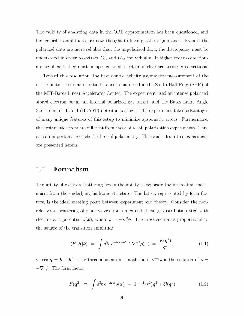
cross section is straightforward. The lowest order amplitudes of the QED perturbative

expansion of the ep-cross section are shown in Fig. 1-1. The form factors are defined

in Sec. 1.1.2 in terms of the nucleon current of the OPE amplitude (a). In an electron

scattering experiment, one needs to take into account radiative corrections in addition

to the OPE. The electron radiative corrections of the next four amplitudes (b)–(e)

are model-independent and can be calculated exactly in terms of GE and GM . The

proton radiative corrections (f)–(h) are suppressed by the mass of the proton, and

the two-photon box (i) and cross (j) amplitudes are suppressed by α2. However, the

model-dependent amplitudes are now being actively re-investigated in an attempt to

reconcile the form factor ratio extraction between polarized and unpolarized data.

(a) Bornamplitude

(b) electronrad. s-peak

(c) electronrad. p-peak

(d) vertexcorrection

(e) vacuumpolarization

(f) vertexcorrection

(g) protonradiation

(h) protonradiation

(i) 2γ boxamplitude

(j) 2γ crossamplitude

Figure 1-1: Diagrams of the lowest-order ep scattering amplitudes.

21

1.1.1 Kinematics

PSfrag replacements

x ∗

x∗y∗

z ∗z∗

θ

θ

φφ

θ∗φ∗

k1k1

k2

k2

p1p1

p2p2

h = ±1

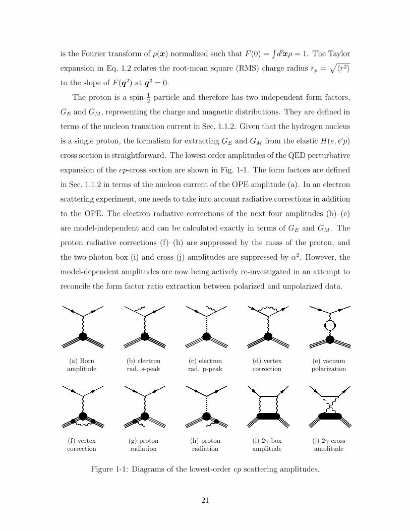
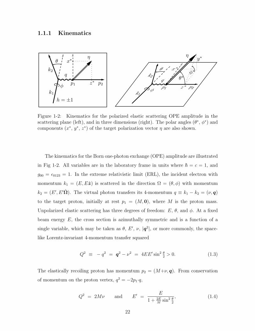
ηη

qq

Figure 1-2: Kinematics for the polarized elastic scattering OPE amplitude in thescattering plane (left), and in three dimensions (right). The polar angles (θ∗, φ∗) andcomponents (x∗, y∗, z∗) of the target polarization vector η are also shown.

The kinematics for the Born one-photon exchange (OPE) amplitude are illustrated

in Fig 1-2. All variables are in the laboratory frame in units where ~ = c = 1, and

g00 = ε0123 = 1. In the extreme relativistic limit (ERL), the incident electron with

momentum k1 = (E, Ez) is scattered in the direction Ω = (θ, φ) with momentum

k2 = (E ′, E ′Ω). The virtual photon transfers its 4-momentum q ≡ k1 − k2 = (ν, q)

to the target proton, initially at rest p1 = (M,0), where M is the proton mass.

Unpolarized elastic scattering has three degrees of freedom: E, θ, and φ. At a fixed

beam energy E, the cross section is azimuthally symmetric and is a function of a

single variable, which may be taken as θ, E ′, ν, |q2|, or more commonly, the space-

like Lorentz-invariant 4-momentum transfer squared

Q2 ≡ − q2 = q2 − ν2 = 4EE ′ sin2 θ2

> 0. (1.3)

The elastically recoiling proton has momentum p2 = (M+ν, q). From conservation

of momentum on the proton vertex, q2 = −2p1·q,

Q2 = 2Mν and E ′ =E

1 + 2EM

sin2 θ2

, (1.4)

22

or in terms of the dimensionless quantity τ ≡ Q2/4M2,

ν2 = τQ2 and q2 = (1 + τ)Q2. (1.5)

The longitudinal polarization of the virtual photon is

ε =(1 + 2(1 + τ) tan2 θ

2

)−1. (1.6)

We also define K ≡ k1 + k2 and P ≡ p1 + p2, and note that K·q = P ·q = 0.

The polarized cross section has additional spin degrees of freedom. We only con-

sider longitudinally polarized electrons with helicity h = ±1, which is equal to the

helicity of the scattered electron in the ERL. The target polarization vector η = (0, η)

is most conveniently represented in the coordinate system of the scattering plane

(x∗, y∗, z∗), where z∗ is in the direction of q, y∗ is in the direction of k1×k2, perpen-

dicular to the scattering plane, and x∗ is in the scattering plane, perpendicular to

z∗, forming a right-handed system. The spin orientation in the polar coordinates is

(θ∗, φ∗), where

x∗ = sin θ∗ cos φ∗, y∗ = sin θ∗ sin φ∗, and z∗ = cos θ∗. (1.7)

The spin of the recoil proton is fixed by conservation of angular momentum. In

the Born approximation, the cross section vanishes for a target polarized along y∗

(Sec. 1.2.6). In the laboratory, the target polarization angle β is defined with respect

to the beam in the scattering plane and positive in the left sector (Sec. 2.3).

The radiative kinematics of Fig. 1-1 (c) and (d) have three additional degrees of

freedom for the outgoing momentum k of the radiated photon. Consequently, the

experimental determination of Q2 from the leptonic vertex Q2l = −(k1−k2)

2 differers

with that from the hadronic vertex Q2h = t = −(p2 − p1)

2. In the following we

use the leptonic vertex for our analysis, Q2 ≡ Q2l . The photon 3-momentum k is

parametrized by the inelasticity v = (k + p2)2 −M2 = 2k·p2, the projection of the

photon momentum along q, τk = k·q/q·p1, and the azimuthal angle φk. The elastic

23

condition Q2 = 2Mν becomes Q2 +v = 2Mν. In terms of these variables, the photon

phase space is [4]

∫d3k

2k0

=

∫ vm

0

dv

4√

λq

∫ τmax

τmin

dτk v

(1 + τk)2

∫ 2π

0

dφk (1.8)

with limits

vm =

√λs

√λm − 2m2Q2 −Q2S

2m2≈ S −Q2 − M2Q2

S, (1.9)

τmaxmin =

v + Q2 ±√

λq

2M2, (1.10)

where

λq = S2x + 4M2Q2, λs = S2 − 4m2M2, λm = Q2(Q2 + 4M2). (1.11)

In terms of R = 2k1·p1 = 2Mk (used interchangeably with v), Rτk = 2k·q. The

Lorentz invariants S = 2k1·p1 and X = 2k2·p2 are the same as those of the OPE

amplitude, and Sx ≡ S −X = Q2 + v.

1.1.2 Form Factors

The Born invariant amplitude contains the transition currents of the electron jµ and

proton Jν joined by the photon propagator gµν/q2,

M = jµ1

q2Jµ, where jµ = −e uk2γ

µuk1 , Jµ = e up2Γµup1 , (1.12)

and u = (√

E+M, σ·p/√

E+M)T χ. Here, σ are the Pauli matrices, and χ a two-

component spinor. The electron has pure Dirac coupling, while the proton vertex is

parametrized by the most general non-parity-violating, Lorentz-invariant conserved

current,

Γµ = F1γµ + κ

2MF2iσ

µνqν . (1.13)

24

The Dirac form factor F1(Q2) describes an extended Dirac particle of which the spin is

preserved in the ERL. The Pauli form factor F2 accounts for the anomalous magnetic

moment of the proton κ = µ− 1 associated with a spin flip.

While F1 and F2 are preferred in Vector Meson Dominance (VMD) models (Sec. 1.3.3)

and in describing the perturbative QCD high Q2 limit of proton structure (Sec. 1.3.1),

the Sachs form factors

GE = F1 − τ κF2 and GM = F1 + κF2 (1.14)

are a more natural description of the nucleon current densities and their coupling to

the virtual photon. Using the Gordon decomposition Γ = γGM + κF2P/2M in the

Breit frame, defined by PB ≡ p1 + p2 = (2EB,0) so that νB = 0,

ΓµB = γµGM + δµ

0MEB

(GE −GM), (1.15)

JB = e χ†p2

(2M GE, iσ×q GM) χp1 . (1.16)

Thus the proton transition current JB(Q2) in the Breit frame corresponds to the

charge and magnetic moment distributions in the proton [5]. The Sachs form factors

GE and GM are the C0 and M1 multipole form factors [6] which couple to longitudinal

and transverse polarization of virtual photon respectively. Accordingly, they normal-

ize to the charge and magnetic moments of the proton, GE(0) = 1 and GM(0) = µ in

units of e and µN , respectively. In contrast to the Dirac and Pauli form factors, the

cross term GEGM vanishes in the unpolarized cross section.

Although the transition current takes on such a simple form in the Breit frame,

the Sachs form factors cannot be rigorously identified as Fourier transforms of spatial

charge and magnetization densities in the proton because the Breit frame varies with

Q2. However, at Q2 M2 the energy transfer is negligible and the identification

of GE(Q2) with the Fourier transform of the charge distribution is valid. Thus the

charge and magnetic radius of the proton can still be extracted from the derivative

of GE and GM at Q2 = 0. Kelly [7] has investigated the use of relativistic inversion

25

to extract spatial densities from the form factors at higher Q2.

1.1.3 Dynamics

The unpolarized elastic p(e, e′)p cross section was first derived by Rosenbluth [8], who

used an effective charge e′(q2) and an effective anomalous magnetic moment µ′(q2)

for F1 and (1+κ)F2, respectively. Dombey [9] and Alkezier [10] did early calculations

of the polarized cross section, which is also given in [11, 6, 4]. From Eq. 1.12, the

Born cross section factorizes into leptonic and hadronic tensors

dσ

dΩ=

σM

L2M

LµνWµν , where σM =

α2 cos2 θ2

4E2 sin4 θ2

E ′

E(1.17)

is the Mott (non-structure) cross section including the recoil factor with corresponding

L2M = LM

µνLµνM = 16M2EE ′ cos2 θ

2. The leptonic and hadronic tensors are

Lµν =∑

h′jµ∗jν =

(2k

(µ1 k

ν)2 + q2gµν

)− ih

[εµν

αβkα1 kβ

2

], (1.18)

W µν =∑

η′Jµ∗Jν =

(G2

MLµνp + κF2(2F1 − (1−τ)κF2)P

µP ν)

(1.19)

−iηα

[2MG2

Mεµναβqβ − 1M

κF2GMεµαβ[γP ν]qβp1γ

],

where a(αbβ)≡aαbβ+aβbα, a[αbβ]≡aαbβ−aβbα, Lµνp = 2p

(µ1 p

ν)2 + q2gµν , and εαβγδ is the

completely antisymmetric tensor.

Both tensors have symmetric (in µ, ν) unpolarized terms and antisymmetric po-

larized terms. Therefore in the Born approximation, dσdΩ

= Σ + h∆, there are no

single-spin asymmetries. The polarized cross section is proportional to the product

P=PbPt of beam and target polarizations and changes sign with either electron or

target spin reversal. From the four different combinations of beam and target spin

configuration, one may extract the polarized and unpolarized cross sections and two

independent false asymmetries.

The unpolarized part of the cross section is

Σ = σM

[(F 2

1 + τ(κF2)2)

+ 2τ(F1 + κF2)2 tan2 θ

2

](1.20)

26

= σM

(G2

E + τG2M

1 + τ+ 2τG2

M tan2 θ2

)(1.21)

= σMτG2

M + εG2E

ε(1 + τ), (1.22)

The transverse and longitudinal response functions are G2M and G2

E, and ε is the

longitudinal polarization of the virtual photon. The polarized cross section is

∆ = −σMvpp1

M·(Kq G2

M + (PK−Kq) GEGM

)· η (1.23)

= σMvp

(K0qG2

M + 1νq×(K×q)GEGM

)· η (1.24)

= σM

(vzz

∗G2M + vxx

∗GEGM

), (1.25)

where

vp = − tan2 θ2/[2M2(1 + τ)],

vz = vp K0|q| = −2τ tan θ2

√1

1+τ+ tan2 θ

2,

vx = vp2M |K|(1 + τ) = −2 tan θ2

√τ

1+τ,

(1.26)

and z∗ and x∗ are the longitudinal and transverse components of the target spin unit

vector with respect to q in the scattering plane. The asymmetry is zero for the normal

component (y∗). This formula is consistent with Donnelly and Raskin [6] except their

response functions lack the factor q2/Q2 = 1 + τ , which is the exact correction to a

relativistic approximation used throughout their derivation, following the method of

Carlson and Gross [11]. Afanasev et al. [4, Eqs. 9–13,17–21] use a simpler form for

the hadronic tensor which gives the same cross section.

The physics asymmetry is

A ≡ σ+ − σ−σ+ + σ−

=∆

Σ=

vzz∗G2

M + vxx∗GEGM

(τG2M + εG2

E) /[ε(1 + τ)](1.27)

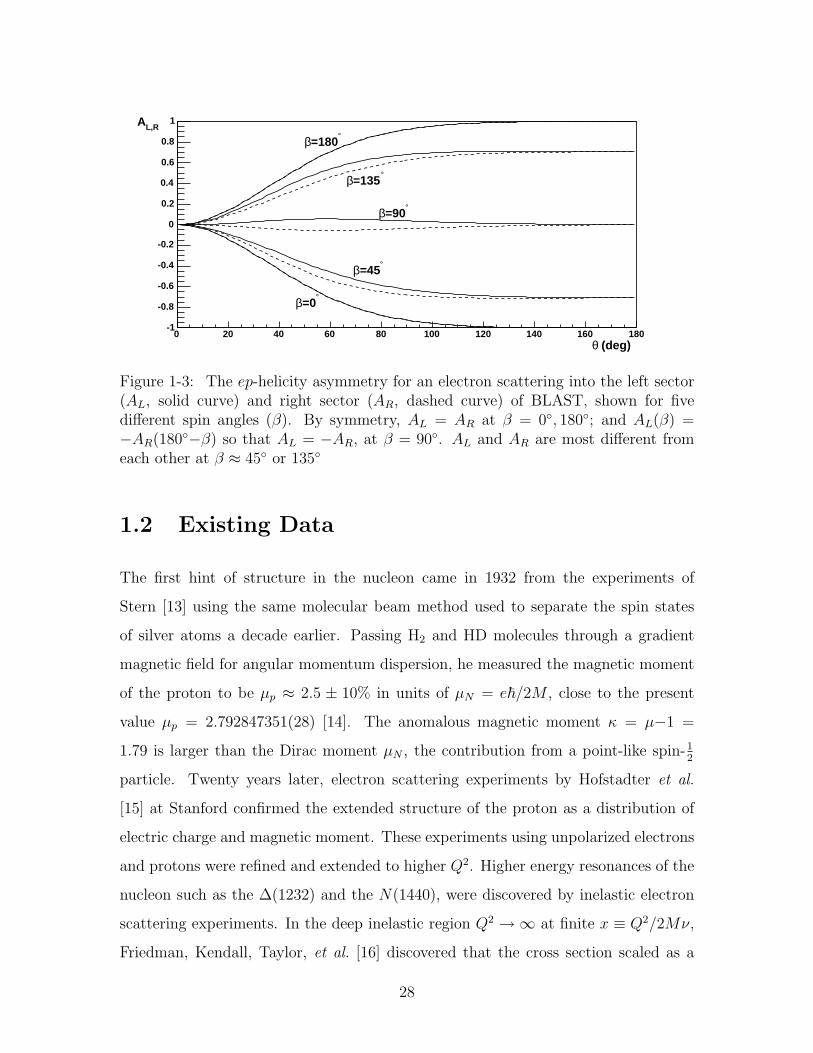
where σh is indexed by the beam helicity h = ±1, and σ+(−η) = σ−(+η). Figure 1-3

shows the asymmetry as a function of θ and the target spin angle β using the Hohler

form factor parametrization [12] as input. The asymmetry goes from 0 at θ = 0

(purely longitudinal) to 100% at θ = 180, confirming that the spin of the electron is

preserved in the ERL.

27

0 20 40 60 80 100 120 140 160 180-1

-0.8

-0.6

-0.4

-0.2

0

0.2

0.4

0.6

0.8

1L,RA

(deg)θ

°=0β

°=45β

°=90β

°=135β

°=180β

Figure 1-3: The ep-helicity asymmetry for an electron scattering into the left sector(AL, solid curve) and right sector (AR, dashed curve) of BLAST, shown for fivedifferent spin angles (β). By symmetry, AL = AR at β = 0, 180; and AL(β) =−AR(180−β) so that AL = −AR, at β = 90. AL and AR are most different fromeach other at β ≈ 45 or 135

1.2 Existing Data

The first hint of structure in the nucleon came in 1932 from the experiments of

Stern [13] using the same molecular beam method used to separate the spin states

of silver atoms a decade earlier. Passing H2 and HD molecules through a gradient

magnetic field for angular momentum dispersion, he measured the magnetic moment

of the proton to be µp ≈ 2.5 ± 10% in units of µN = e~/2M , close to the present

value µp = 2.792847351(28) [14]. The anomalous magnetic moment κ = µ−1 =

1.79 is larger than the Dirac moment µN , the contribution from a point-like spin-12

particle. Twenty years later, electron scattering experiments by Hofstadter et al.

[15] at Stanford confirmed the extended structure of the proton as a distribution of

electric charge and magnetic moment. These experiments using unpolarized electrons

and protons were refined and extended to higher Q2. Higher energy resonances of the

nucleon such as the ∆(1232) and the N(1440), were discovered by inelastic electron

scattering experiments. In the deep inelastic region Q2 →∞ at finite x ≡ Q2/2Mν,

Friedman, Kendall, Taylor, et al. [16] discovered that the cross section scaled as a

28

function of the momentum fraction of the struck parton x, independent of Q2. This

confirmed the partonic structure of the nucleon and the existence of quarks.

In the last decade, a new generation of polarization experiments have measured

µGE/GM to higher precision; however the results are in conflict with the unpolarized

data. There has been a considerable effort to reconcile these two sets of data. This

section provides a summary of the different experiments used to measure the form

factors of the proton.

1.2.1 Rosenbluth Separation

The standard method of extracting GE(Q2) and GM(Q2) from the unpolarized elastic

p(e, e′) cross section is by a Rosenbluth separation. At a given Q2, the cross section

must be measured at different kinematics in order to separate GE from GM . The only

other parameter to vary is the beam energy E. In terms of the Dirac and Pauli form

factors F1 and F2, the cross section of Eq. 1.20 has the from aF 21 +bF1F2 +cF 2

2 . Early

extractions were done using the “ellipse method,” by plotting the elliptical constraints

on F1 and F2 of cross section measurements at different energies. The form factors F1

and F2 were extracted from the intersection of all ellipses, although the same result

could have been obtained algebraically.

A practical advantage of the Sachs form factors GE and GM is the disappearance

of this cross term. The reduced cross section

dσ

dΩ

ε(1 + τ)

σM

≡ σR = τG2M + εG2

E (1.28)

is linear in ε, so τGM and GE are the intercept and slope, respectively, of σR as

a function of ε. Early separations also fit reduced cross sections as a function of

tan2( θ2) or cot2( θ

2), which are also linear. Assuming that GE and GM are of the same

order of magnitude, the factor τ = Q2/4M2 implies that the reduced cross section is

dominated by GE at low Q2 and by GM at high Q2, making Rosenbluth separations

difficult at these extremes. This is reflected in the unpolarized data.

Initial measurements of the Dirac and Pauli form factors performed at the Stanford

29

Linear Accelerator by Hofstadter [15] confirmed the extended structure of the proton.

Their results of both F1 and F2 were consistent with dipole form factors, which

correspond to exponential charge and magnetic distributions,

ρ(r) = e−r/r0 , (1.29)

each with an RMS radius of 0.75 fm. Subsequent separations of GE and GM [17, 18, 19]

confirmed the dipole form

GE(Q2) = 1µGM(Q2) = GD(Q2) ≡ 1

(1 + Q2/Λ2)2, (1.30)

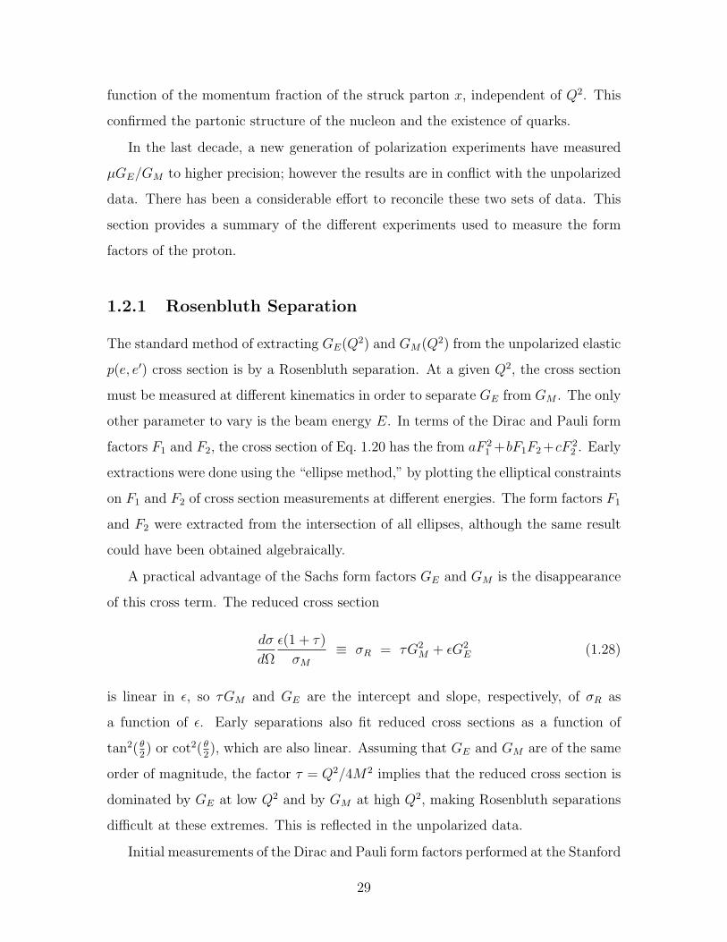
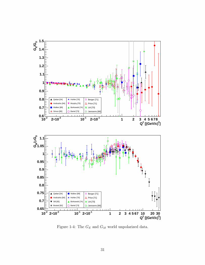
with Λ2 = 0.71 (GeV/c)2. Usually GE and GM are quoted in units of GD. The world

unpolarized data of GE and GM , normalized to GD are shown in Fig. 1-4

1.2.2 Proton RMS Radius

An early physics goal of elastic scattering since the first measurements of Hofstadter

was to determine the RMS charge radius rp of the proton. This is a fundamental

static property of the nucleon as is its magnetic moment. It is also an important

physics input into the QED calculation of the hydrogen Lamb Shift, a precision test

of QED. The importance of rp is further discussed in [20].

The ideal method of extracting rp from unpolarized data is to do a Rosenbluth

separation of GE and GM , and fit for the slope of GE at Q2 = 0 to get rp. However

because the cross section is dominated by GE at low Q2, one must make the assump-

tion that µGE/GM ≈ 1. Also, rp is determined strictly by the behavior of GE near

Q2 = 0 regardless of the shape of form factors at higher Q2, and the slope must be

measured at Q2 (~c/rp)2 ≈ 0.05 (GeV/c)2, well below any structure due to the

shape of the proton. From the dipole form factor, rp =√

12/Λ2 = 0.811 fm, a little

short of the currently accepted value of rp = 0.8750(68) fm [14].

Early unpolarized data were taken mostly at low Q2 and were sensitive to rp.

Hand et al. [21] reanalyzed the results of eight early experiments at Q2 < 1.8 (GeV/c)2

30

]2

[(GeV/c)2Q

-210 -210×2 -110 -110×2 1 2 3 4 5 6 78

D/G

EG

0.6

0.7

0.8

0.9

1

1.1

1.2

1.3

1.4

1.5

Qattan [04]

Andivahis [94]

Walker [89]

Simon [80]

Hohler [76]

Murphy [75]

Borkowski [74]

Bartel [73]

Berger [71]

Price [71]

Litt [70]

Janssens [66]

]2

[(GeV/c)2Q

-210 -210×2 -110 -110×2 1 2 3 4 5 67 10 20 30

DGµ/

MG

0.65

0.7

0.75

0.8

0.85

0.9

0.95

1

1.05

1.1

Qattan [04]

Andivahis [94]

Sill [93]

Bosted [92]

Walker [89]

Hohler [76]

Borkowski [74]

Bartel [73]

Berger [71]

Price [71]

Litt [70]

Janssens [66]

Figure 1-4: The GE and GM world unpolarized data.

31

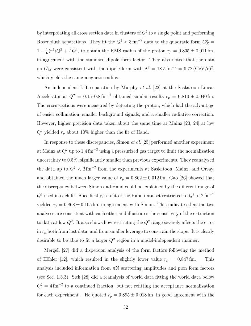
by interpolating all cross section data in clusters of Q2 to a single point and performing

Rosenbluth separations. They fit the Q2 < 3 fm−2 data to the quadratic form GpE =

1 − 16〈r2〉Q2 + AQ4, to obtain the RMS radius of the proton rp = 0.805 ± 0.011 fm,

in agreement with the standard dipole form factor. They also noted that the data

on GM were consistent with the dipole form with Λ2 = 18.5 fm−2 = 0.72 (GeV/c)2,

which yields the same magnetic radius.

An independent L-T separation by Murphy et al. [22] at the Saskatoon Linear

Accelerator at Q2 = 0.15–0.8 fm−2 obtained similar results rp = 0.810 ± 0.040 fm.

The cross sections were measured by detecting the proton, which had the advantage

of easier collimation, smaller background signals, and a smaller radiative correction.

However, higher precision data taken about the same time at Mainz [23, 24] at low

Q2 yielded rp about 10% higher than the fit of Hand.

In response to these discrepancies, Simon et al. [25] performed another experiment

at Mainz at Q2 up to 1.4 fm−2 using a pressurized gas target to limit the normalization

uncertainty to 0.5%, significantly smaller than previous experiments. They reanalyzed

the data up to Q2 < 2 fm−2 from the experiments at Saskatoon, Mainz, and Orsay,

and obtained the much larger value of rp = 0.862 ± 0.012 fm. Gao [26] showed that

the discrepancy between Simon and Hand could be explained by the different range of

Q2 used in each fit. Specifically, a refit of the Hand data set restricted to Q2 < 2 fm−2

yielded rp = 0.868± 0.105 fm, in agreement with Simon. This indicates that the two

analyses are consistent with each other and illustrates the sensitivity of the extraction

to data at low Q2. It also shows how restricting the Q2 range severely affects the error

in rp both from lost data, and from smaller leverage to constrain the slope. It is clearly

desirable to be able to fit a larger Q2 region in a model-independent manner.

Mergell [27] did a dispersion analysis of the form factors following the method

of Hohler [12], which resulted in the slightly lower value rp = 0.847 fm. This

analysis included information from πN scattering amplitudes and pion form factors

(see Sec. 1.3.3). Sick [28] did a reanalysis of world data fitting the world data below

Q2 = 4 fm−2 to a continued fraction, but not refitting the acceptance normalization

for each experiment. He quoted rp = 0.895± 0.018 fm, in good agreement with the

32

most recent atomic physics extraction [20]. His analysis included Coulomb distortion

effects, arising from multiple soft photons transfered along with the hard virtual

photon of momentum transfer q. This effect was shown to increase the radius by about

0.01 fm. The current standard accepted value of the proton RMS radius, influenced

by these fits, is rp = 0.8750(68) fm [14].

There are new proposals for precision measurements of rp. RpEX, [26] the sister

experiment of this experiment was proposed to measure both the form factor ratio

and relative cross section at 22 points between 0.13 < Q2 < 2.26 fm−2. These

would be used in conjunction with polarization data measured in the same range to

extract GE(Q2), normalized by GE(0) = 1. The proposal projected an increase in the

precision of rp by a factor of 3, compared to the combined world data.

Another experiment, Exp. R-98-003 [29], is being carried out at the Paul Scherrer

Institute (PSI) to measure the 2S Lamb shift from muonic hydrogen (µp). The muon

is more massive than the electron, and its wave function has more overlap with the

proton. Therefore, the muonic Lamb shift is more sensitive to the proton radius, and

the extraction of rp has a projected uncertainty of 0.1%, a factor of 20 increase in

precision.

1.2.3 Higher Q2 Unpolarized Data

Subsequent unpolarized experiments focused on extending the measurements of GE

and GM to higher Q2 and higher precision, with higher beam energy and more sophis-

ticated detectors. Two physics motivations of these experiments were: a) the investi-

gation whether µGE/GM ≈ 1 scaling continues to higher Q2, and b) the asymptotic

dependence of F1 and F2 as predicted by perturbative QCD.

Some dedicated L-T separation experiments measured cross sections at many val-

ues of ε for each Q2 point, while other data were taken simply as calibration mea-

surements for other electron scattering experiments. For data at Q2 > 10 (GeV/c)2,

the electric contribution to the cross section is so small that GM could be extracted

without performing a Rosenbluth separation. Other experiments assumed scaling

(GE = GM/µ) to extract GE and GM . Some experiments combined their data with

33

earlier experiments in order to perform separations. Thus although some experi-

ments can be presented as independent measurements, a more meaningful picture

comes from global analyses such as those of Walker et al. [30] and Arrington [31].

The following is a description of the data used in those references.

Two experiments carried out at the Cambridge Electron Accelerator (CEA), one

by Goitein et al. [32] at forward angles, and the other by Price et al. [18] at backward

angles, were combined to extract GE and GM at Q2 = 7–45 fm−2, in the same range

as the analysis of Hand [21]. From the d(e, e′p) data of Hanson [33], the ratio of the

deuteron quasielastic to proton elastic cross section was 0.80–0.95 depending on Q2.

An independent L-T separation was performed at the 2.5 (GeV/c) Bonn syn-

chrotron by Berger et al. [34] in approximately the same Q2 range. They measured

cross sections at multiple energies for each Q2 value, most notably 15 energies at

Q2 = 0.58 (GeV/c)2, and found good linear dependence. They reported µGE/GM to

drop significantly below 1.

Another independent L-T separation was also done at DESY by Bartel et al.

[35] at Q2 = 0.67–3.0 (GeV/c)2. Cross sections were taken with one spectrometer at

forward angles and the other one at 86. These data also showed a significant drop

in µGE/GM . In addition, the proton was detected at forward angles for some Q2

values. This was also compared with d(e, e′p) to show that deuteron binding effects

in the quasielastic cross section were small. Earlier experiments at DESY [36, 17, 37]

measured cross section data up to Q2 = 9 (GeV/c)2, but at only a single beam energy.

The bulk of the proton unpolarized cross section data has come from SLAC.

Janssens et al. [38] did an extensive set of L-T separations in the range Q2 = 4–30 fm−2

using the 1 (GeV/c) spectrometer. Litt et al. [39] also did independent L-T separa-

tions at higher Q2 values (1.0–3.75 (GeV/c)2), and the results were consistent with

scaling (µGE/GM ≈ 1). In the same experiment, Kirk et al. [19] measured GM to

Q2 = 25 (GeV/c)2 under the assumption of continued scaling (µGE/GM ≈ 1).

There are four other cross section sets with insufficient data for independent L-T

separations. Stein et al. [40] measured the cross section at Q2 = 0.1–1.8 (GeV/c)2 with

beam energy up to 20 GeV as part of a comprehensive DIS program with a 20 GeV

34

electron spectrometer fixed at θ = 4. Rock et al. [41] measured the cross section at

Q2 = 2.5–10 (GeV/c)2 as calibration for d(e, e′n) cross section measurements. Bosted

et al. [42] measured the same, but using a θ = 180 spectrometer, for which kinematics

the cross section only depends on GM . Sill et al. [43] repeated the measurements of

Kirk et al. up to even higher Q2 (31 (GeV/c)2) in search of scaling predicted by pQCD.

Two more recent L-T separations have been performed at SLAC. Andivahis et

al. [44] doubled the Q2 range of Rosenbluth separations to 8.8 (GeV/c)2, taking

data with both the 1.6 and 8 GeV spectrometers. The spectrometers were cross-

normalized with a simultaneous measurement at the same kinematics. The world

data for Q2 > 3 (GeV/c)2 is dominated by this single experiment. An earlier exper-

iment by Walker et al. [30] measured GE and GM at the four points Q2 = 1.0, 2.0,

2.5, and 3.0 (GeV/c)2 with a single detector, the 8 GeV spectrometer, avoiding the

problems of normalization. However Ref. [31] claims the data for θ < 20 did not

have the proper corrections applied, as was done in Ref. [44].

The latest unpolarized data have been taken at Jefferson Lab. Dutta et al. [45]

(JLab Exp. E91-013) measured hydrogen cross sections as part of an investigation

of nuclear transparency and the nuclear spectral functions of carbon, iron, and gold

nuclei. Experiment E94-110 [46, 47] measured the elastic hydrogen cross section

at 28 points in the range 0.4 < Q2 < 5.5 (GeV/c)2 as part of a program to measure

R = σL/σT in the resonance region. Finally, experiment E01-001 [48] was a dedicated

high precision Rosenbluth separation of the hydrogen form factors at Q2 = 2.64, 3.20,

and 4.10 (GeV/c)2. In this experiment, the proton was detected instead of the elec-

tron to minimize systematic errors. At fixed Q2, the recoil proton has the same

momentum regardless of the beam energy, thus avoiding uncertainty due to momen-

tum dependence of the spectrometer acceptance. Also, the cross section dσ/dΩp for

detecting protons is much larger and slower-varying than that of the electron dσ/dΩe

because the proton angle does not change as rapidly. The experiment used the second

spectrometer to simultaneously measure the cross section at Q2 = 0.5 (GeV/c)2 for

normalization purposes, although these data were not reported in Ref. [48].

35

1.2.4 Polarized Data

Recent advances in polarized beams, polarized targets, and polarimetry have made

possible a new generation of precision measurements of µGE/GM . Such experiments

benefit from interference terms between GE and GM in the polarized response func-

tions. The extra spin degree of freedom allows for direct measurement of µGE/GM

at a single beam energy.

In the extreme relativistic limit (ERL), the electron helicity is conserved, and it

is much easier to prepare polarized beams than to detect the scattered electron po-

larization. Furthermore, in the OPE approximation, single polarization asymmetries

with either polarized beam and unpolarized target or vice versa are parity-violating

and very small. This leaves two double-polarization measurements from ep-elastic

scattering: ~p(~e, e′p) and p(~e, e′~p).

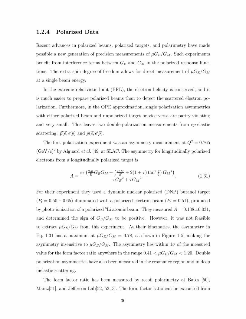
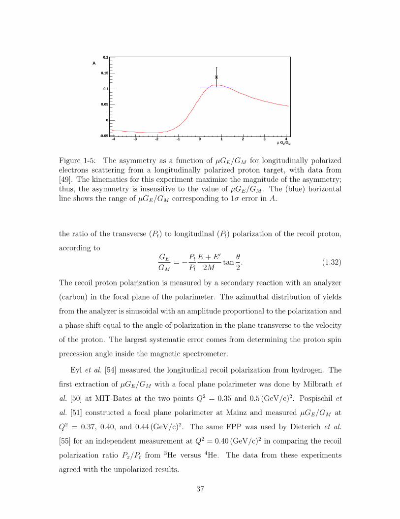
The first polarization experiment was an asymmetry measurement at Q2 = 0.765

(GeV/c)2 by Alguard et al. [49] at SLAC. The asymmetry for longitudinally polarized

electrons from a longitudinally polarized target is

A =ετ(

2ME

GEGM +(

2τME

+ 2(1 + τ) tan2 θ2

)GM

2)

εGE2 + τGM

2 . (1.31)

For their experiment they used a dynamic nuclear polarized (DNP) butanol target

(Pt = 0.50 – 0.65) illuminated with a polarized electron beam (Pe = 0.51), produced

by photo-ionization of a polarized 6Li atomic beam. They measured A = 0.138±0.031,

and determined the sign of GE/GM to be positive. However, it was not feasible

to extract µGE/GM from this experiment. At their kinematics, the asymmetry in

Eq. 1.31 has a maximum at µGE/GM = 0.78, as shown in Figure 1-5, making the

asymmetry insensitive to µGE/GM . The asymmetry lies within 1σ of the measured

value for the form factor ratio anywhere in the range 0.41 < µGE/GM < 1.20. Double

polarization asymmetries have also been measured in the resonance region and in deep

inelastic scattering.

The form factor ratio has been measured by recoil polarimetry at Bates [50],

Mainz[51], and Jefferson Lab[52, 53, 3]. The form factor ratio can be extracted from

36

M/GE Gµ-4 -3 -2 -1 0 1 2 3 4

-0.05

0

0.05

0.1

0.15

0.2

A

Figure 1-5: The asymmetry as a function of µGE/GM for longitudinally polarizedelectrons scattering from a longitudinally polarized proton target, with data from[49]. The kinematics for this experiment maximize the magnitude of the asymmetry;thus, the asymmetry is insensitive to the value of µGE/GM . The (blue) horizontalline shows the range of µGE/GM corresponding to 1σ error in A.

the ratio of the transverse (Pt) to longitudinal (Pl) polarization of the recoil proton,

according toGE

GM

= −Pt

Pl

E + E ′

2Mtan

θ

2. (1.32)

The recoil proton polarization is measured by a secondary reaction with an analyzer

(carbon) in the focal plane of the polarimeter. The azimuthal distribution of yields

from the analyzer is sinusoidal with an amplitude proportional to the polarization and

a phase shift equal to the angle of polarization in the plane transverse to the velocity

of the proton. The largest systematic error comes from determining the proton spin

precession angle inside the magnetic spectrometer.

Eyl et al. [54] measured the longitudinal recoil polarization from hydrogen. The

first extraction of µGE/GM with a focal plane polarimeter was done by Milbrath et

al. [50] at MIT-Bates at the two points Q2 = 0.35 and 0.5 (GeV/c)2. Pospischil et

al. [51] constructed a focal plane polarimeter at Mainz and measured µGE/GM at

Q2 = 0.37, 0.40, and 0.44 (GeV/c)2. The same FPP was used by Dieterich et al.

[55] for an independent measurement at Q2 = 0.40 (GeV/c)2 in comparing the recoil

polarization ratio Px/Pt from 3He versus 4He. The data from these experiments

agreed with the unpolarized results.

37

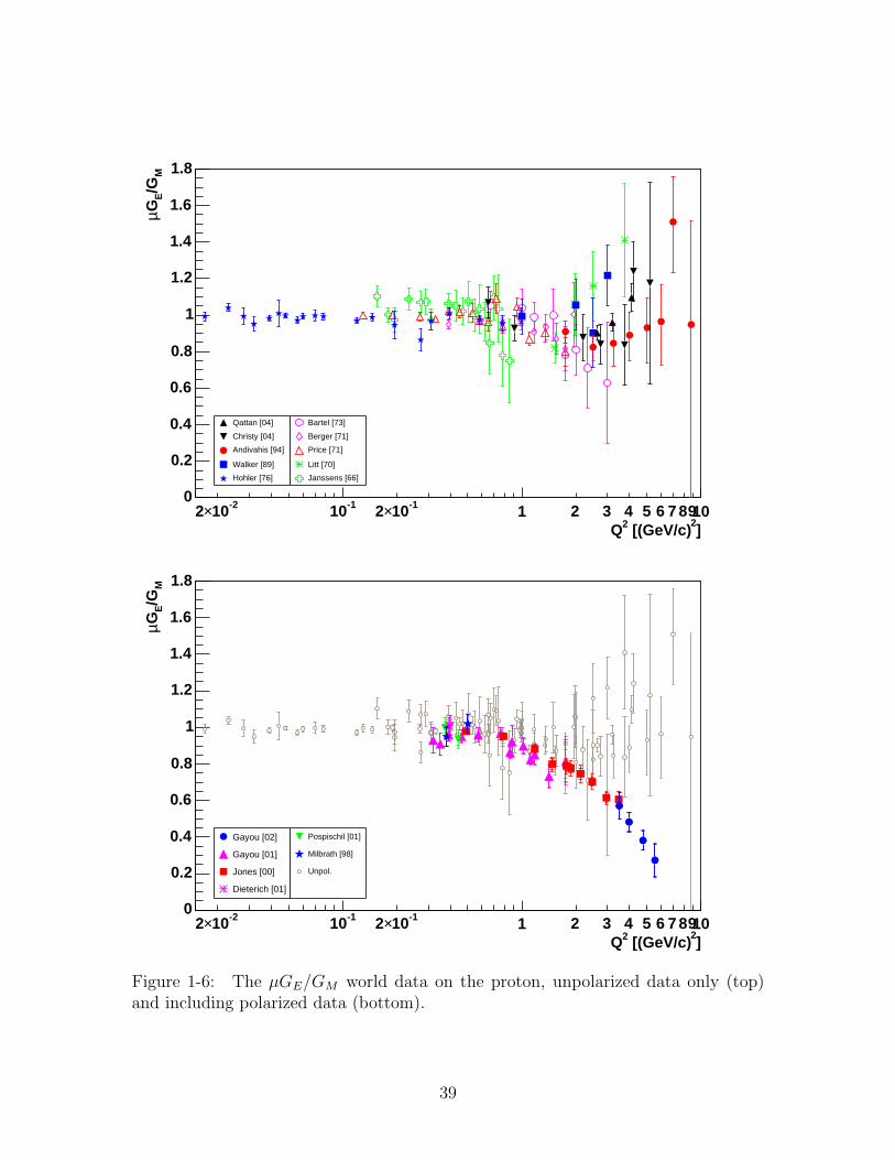
The FPP measurements were extended to higher Q2 at Jefferson Lab Hall A

by Jones et al. [2] with the unexpected result of a dramatic linear decrease in the

form factor ratio down to µGE/GM = 0.6 at Q2 = 3.5 (GeV/c)2. These results

were reproduced in a subsequent calibration of the FPP [53] for two other exper-

iments on D(~γ, ~p)n and H(~γ, ~p)π0. Gayou et al. [3] extended the measurement to

Q2 = 5.5 (GeV/c)2, and observed the same trend. The form factor ratio continued to

decrease linearly down to 0.27 at Q2 = 5.5 (GeV/c)2. There is another experiment

approved for JLab Hall C to extend the range to Q2 = 9 (GeV/c)2. The world data

of the form factor ratio are shown in Fig. 1-6

The discrepancy between FPP and unpolarized data has renewed interest in the

proton form factors. It prompted considerable theoretical activity, both to reconcile

the polarized and unpolarized data (Sect. 1.2.6), and to understand the intriguing

Q2 dependence of µGE/GM (Sect. 1.3). Experiment E01-001 [48] was performed

at Jefferson Lab to test for possible systematic effects in the previous unpolarized

experiments, but the results were consistent with the unpolarized world data. A

whole new set of experiments have been proposed to test for higher-order processes

which may contribute to this discrepancy.

1.2.5 Global Analysis

Many global fits to the world data have been performed [21, 18, 34, 25, 30, 56, 57, 31,

58, 59]. In addition, there are fits to theoretical models which will be discussed in the

next section. We consider here the most recent fits. Walker et al. [30] extracted GE

and GM at 17 values of Q2 from the world data with improved radiative corrections.

They also fit a normalization constant for each of the 11 experiments. Bosted [56] fit

this global analysis to an inverse polynomial in Q =√

Q2, and obtained the results

GE(Q2) =1

1 + 0.62Q + 0.68Q2 + 2.80Q3 + 0.83Q4, (1.33)

GM(Q2)

µ=

1

1 + 0.35Q + 2.44Q2 + 0.50Q3 + 1.04Q4 + 0.34Q4(1.34)

38

]2

[(GeV/c)2Q

-210×2 -110 -110×2 1 2 3 4 5 6 7 8910

M/G

EGµ

0

0.2

0.4

0.6

0.8

1

1.2

1.4

1.6

1.8

Qattan [04]

Christy [04]

Andivahis [94]

Walker [89]

Hohler [76]

Bartel [73]

Berger [71]

Price [71]

Litt [70]

Janssens [66]

]2

[(GeV/c)2Q

-210×2 -110 -110×2 1 2 3 4 5 6 7 8910

M/G

EGµ

0

0.2

0.4

0.6

0.8

1

1.2

1.4

1.6

1.8

Gayou [02]

Gayou [01]

Jones [00]

Dieterich [01]

Pospischil [01]

Milbrath [98]

Unpol.

Figure 1-6: The µGE/GM world data on the proton, unpolarized data only (top)and including polarized data (bottom).

39

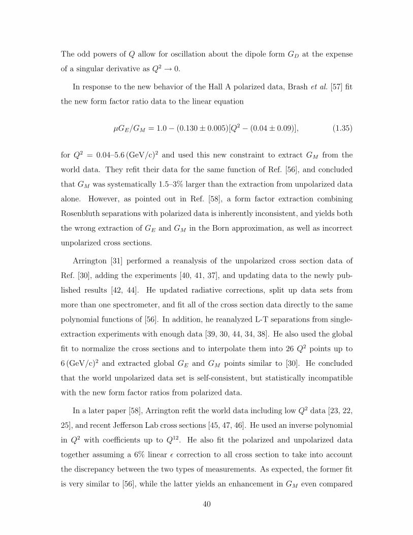
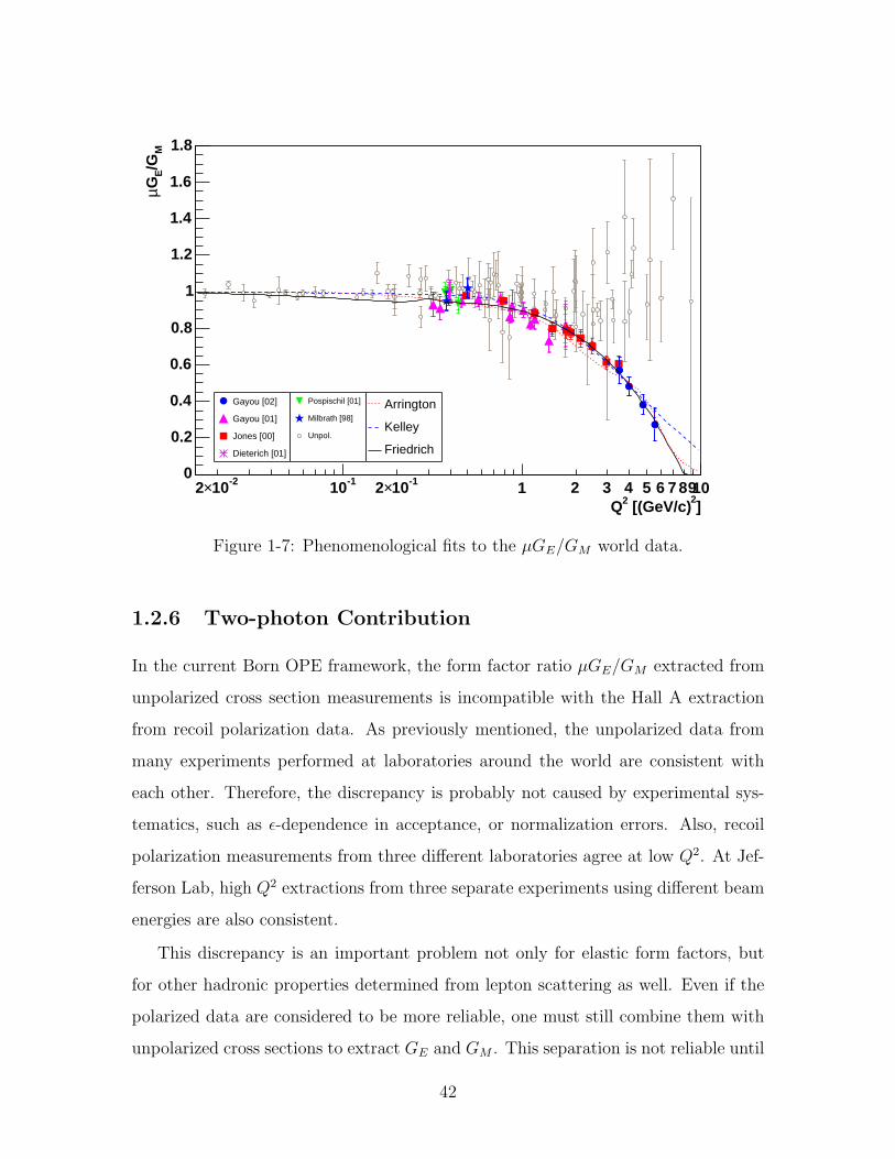
The odd powers of Q allow for oscillation about the dipole form GD at the expense

of a singular derivative as Q2 → 0.

In response to the new behavior of the Hall A polarized data, Brash et al. [57] fit

the new form factor ratio data to the linear equation

µGE/GM = 1.0− (0.130± 0.005)[Q2 − (0.04± 0.09)], (1.35)

for Q2 = 0.04–5.6 (GeV/c)2 and used this new constraint to extract GM from the

world data. They refit their data for the same function of Ref. [56], and concluded

that GM was systematically 1.5–3% larger than the extraction from unpolarized data

alone. However, as pointed out in Ref. [58], a form factor extraction combining

Rosenbluth separations with polarized data is inherently inconsistent, and yields both

the wrong extraction of GE and GM in the Born approximation, as well as incorrect

unpolarized cross sections.

Arrington [31] performed a reanalysis of the unpolarized cross section data of

Ref. [30], adding the experiments [40, 41, 37], and updating data to the newly pub-

lished results [42, 44]. He updated radiative corrections, split up data sets from

more than one spectrometer, and fit all of the cross section data directly to the same

polynomial functions of [56]. In addition, he reanalyzed L-T separations from single-

extraction experiments with enough data [39, 30, 44, 34, 38]. He also used the global

fit to normalize the cross sections and to interpolate them into 26 Q2 points up to

6 (GeV/c)2 and extracted global GE and GM points similar to [30]. He concluded

that the world unpolarized data set is self-consistent, but statistically incompatible

with the new form factor ratios from polarized data.

In a later paper [58], Arrington refit the world data including low Q2 data [23, 22,

25], and recent Jefferson Lab cross sections [45, 47, 46]. He used an inverse polynomial

in Q2 with coefficients up to Q12. He also fit the polarized and unpolarized data

together assuming a 6% linear ε correction to all cross section to take into account

the discrepancy between the two types of measurements. As expected, the former fit

is very similar to [56], while the latter yields an enhancement in GM even compared

40

to [57].

Kelly [59] fit both polarized and unpolarized data to the simple form

GE(Q2) =1− (0.24± 0.12)

1 + (10.98± 0.19)τ + (12.82± 1.1)τ 2 + (21.97± 6.8)τ 3(1.36)

GM(Q2)

µ=

1 + (0.12± 0.04)

1 + (10.97± 0.11)τ + (18.86± 0.28)τ 2 + (6.55± 1.2)τ 3(1.37)

This gives the correct 1/Q4 dependence at high Q2, is well behaved as Q2 → 0, and

gives the RMS proton radius rp = 0.863 ± 0.004 in agreement with the currently

accepted value.

Motivated by a bump structure at Q2 ≈ 0.2–0.3 (GeV/c)2 in the neutron electric

form factor, Friedrich and Walcher [60] have put forth a phenomenological model of

the form factors

GN(Q2) = Gs(Q2) + abQ

2Gb(Q2). (1.38)

The model parametrizes the smooth high Q2 dependence with a pair of dipoles,

Gs(Q2) =

a10

(1 + Q2/a20)2+

a11

(1 + Q2/a21)2, (1.39)

and adds a Gaussian bump at low Q2,

Gb(Q2) = e

−12

“Q−Qb

σb

”2

+ e−1

2

“Q+Qb

σb

”2

, (1.40)

where Q =√

Q2. The second exponential is small and restores the analyticity of

G(Q2) as Q2 → 0. Two dipoles were needed in order to get the right asymptotic Q2

dependence of the form factors, but their amplitudes are related by the normalization

at Q2 = 0, satisfying a10 + a11 = GN(0). They discovered that not only GnE, but also

the “standard” form factors GpE, Gp

M , and GnM fit well to this ansatz. Noting that the

bump has the effect of shifting charge to the outside of the nucleon, they give it the

physical interpretation of a pion cloud. The fits of Arrington, Kelley, and Friedrich

and Walcher are shown in Fig. 1-7.

41

]2

[(GeV/c)2Q

-210×2 -110 -110×2 1 2 3 4 5 6 7 8910

M/G

EGµ

0

0.2

0.4

0.6

0.8

1

1.2

1.4

1.6

1.8

Gayou [02]

Gayou [01]

Jones [00]

Dieterich [01]

Pospischil [01]

Milbrath [98]

Unpol.

Arrington

Kelley

Friedrich

Figure 1-7: Phenomenological fits to the µGE/GM world data.

1.2.6 Two-photon Contribution

In the current Born OPE framework, the form factor ratio µGE/GM extracted from

unpolarized cross section measurements is incompatible with the Hall A extraction

from recoil polarization data. As previously mentioned, the unpolarized data from

many experiments performed at laboratories around the world are consistent with

each other. Therefore, the discrepancy is probably not caused by experimental sys-

tematics, such as ε-dependence in acceptance, or normalization errors. Also, recoil

polarization measurements from three different laboratories agree at low Q2. At Jef-

ferson Lab, high Q2 extractions from three separate experiments using different beam

energies are also consistent.

This discrepancy is an important problem not only for elastic form factors, but

for other hadronic properties determined from lepton scattering as well. Even if the

polarized data are considered to be more reliable, one must still combine them with

unpolarized cross sections to extract GE and GM . This separation is not reliable until

42

the form factor contributions to the cross section are known well enough to reconcile

the two methods [58]. While the current Rosenbluth separations give an adequate

parameterization of the cross section data, it is not meaningful to compare the ex-

tracted form factors with theoretical predictions. Another unresolved question is why

the systematic deviation of the unpolarized cross sections is linear in ε, conspiring to

give false confidence in the Rosenbluth extraction.

The most likely candidate to resolve this discrepancy is the two photon exchange

contribution from the box and cross diagrams of Fig. 1-1. This effect along with the

other radiative effects must be corrected for in the extraction of the form factors,

which are defined as matrix elements in the OPE approximation. However, the two

photon effect is model-dependent and difficult to calculate. Although these effects

had been considered as early as in the 1960’s [61], most unpolarized experiments

were radiatively corrected within the famework of Mo & Tsai [62], in which peaking

approximations were used for q → 0 for one of the photons. The non-infrared diver-

gent parts of the two-photon-exchange were even recently thought to be less than 1%

[30, 63]. It has been shown that Coulomb distortion effects, arising from higher order

diagrams with a hard virtual photon of momentum q and one or more soft virtual

photons, have little effect on Rosenbluth separations [64].

The two-photon exchange term is equivalent to double virtual Compton scattering,

with the virtual photons coupled to the scattered electron. This is complicated by the

fact that the intermediate nucleon can be in any excited state, so that the amplitude

is not just a function of the nucleon form factors. There have been many recent

attempts to describe the effect qualitatively and quantitatively. They have had some

success in reconciling the two methods. However, there are still conflicting statements

among the authors, and a full calculation using realistic structure functions has yet

to be done.

Guichon and Vanderhaeghen [65] developed a framework for the comparison of two

photon effects between polarized and unpolarized experiments. Factoring all higher

order scattering amplitudes into the nuclear current Γ, the most general current

respecting Lorentz, parity, and charge conjugation invariance for a spin 1/2 particle

43

is

Γµ = GMγµ − F2P µ

M+ F3

γ·K P µ

M2, (1.41)

where GM , F2, and F3 are complex functions of Q2 and ε, which equal GM , F2,

and 0 respectively in the Born approximation. GE is defined analogous to Eq. 1.14.

Using standard techniques, they computed both the unpolarized cross section and

recoil polarization from this nucleon current. The form factor ratios, as extracted

from the unpolarized and polarized cross sections, both had corrections containing

the dimensionless two-photon exchange characterization

Y2γ(Q2, ε) = R

(K·PF3

M2|GM |

). (1.42)

Using the difference between polarized and unpolarized extraction of µGE/GM , they

were able to extract Y2γ and the corrected Born OPE form factor ratio. Y2γ turned

out to be a small correction (2–4% depending on Q2) with very little ε dependence,

and the actual µGE/GM was a little higher than, but very close to the polarized

results. Thus the two-photon effects were shown not to alter the linearity of the

Rosenbluth separation. A similar analysis also using e−p and e+p data to separate

GE and GM has also been done [66]. The Y2γ contribution is expected to change sign

when switching between e−p and e+p scattering.

In a general analysis of model-independent properties of two-photon exchange,

Rekalo and Tomasi-Gustafsson [67] started with the same nucleon current as Eq. 1.41.

However, taking into account C-invariance of the electromagnetic interaction of had-

rons, they showed that the first two terms could only involve an odd number of

photons, while the third term involved only an even number of photons. Thus the

phases of GM and F2 were of order α2 and so these were essentially the elastic form

factors. They also confirmed that the amplitudes of GM , F2, and F3 should be the

same for both e−p and e+p scattering. In addition, applying crossing symmetry

between the s-channel (e+e− → pp) and the t-channel (ep → ep), they concluded

that the 1γ-2γ interference contribution should be nonlinear in ε and depend on the

44

variable x =√

(1 + ε)/(1− ε) to first order at least.

The first model-dependent calculation of the two photon effect, by Blunden, Mel-

nitchouk, and Tjon [68] assumed the intermediate nucleon state to stay in the ground

state, with both γp interactions described by the standard proton current operator

of Eq. 1.13. They used monopole form factors GE = GM/µ = G ≡ (1 + Q2/Λ2)−1 in

their calculation. The resulting correction was about 2% in addition to the approxi-

mations of Mo and Tsai [62]. It was almost linear in ε, with slope increasing slightly

with Q2. Thus this calculation was able to explain half of the discrepancy between

polarized and unpolarized form factor ratios.

Chen et al. [69] evaluated the two photon exchange contribution in a partonic

model. The intermediate nucleon included excited states and was modeled with

generalized parton distributions (GPD), which are also useful for describing Virtual

Compton Scattering (VCS). Using input of µGE/GM from the polarized JLab data,

they were able to reproduce the approximate ε-dependence of the unpolarized cross

sections of Ref. [44]. The two-photon exchange contribution increased the slope of

µGE/GM(ε) as desired, but also introduced nonlinearities into the ε dependence.

They also predict the cross section e+/e- ratio for 2 < Q2 < 5 (GeV/c) to be 0.98 at

large ε, crossing 1 at about ε = 0.35. While a full extraction of GE and GM within

this model still needs to be done, this work appears to resolve most of the discrepancy

between the form factor ratio extracted from unpolarized and polarized data.

Experimentally, the effects of the two photon exchange diagram are accessible

through its possible nonlinear ε-dependence, or its C-odd and T -odd (parity con-

serving) properties [70]. Experiments of all three types have been carried out in the

past with limited precision, and new precision measurements of each have been pro-

posed. Although there have been many single-experiment Rosenbluth separations,

the ε ranges were typically insufficient for a conclusive test of linearity. There is

a Jefferson Lab proposal to do a high precision test of linearity at Q2 = 1.12 and

2.56 (GeV/c)2 of the Rosenbluth cross section [71], and also in the recoil polariza-

tions Px and Py [72].

The e± cross sections are identical except for a sign change in the interference

45

between the one and two-photon exchange amplitudes (C-odd). Therefore, the ratio

R = σ(e+p)/σ(e−p) is highly sensitive to the two-photon effect. Previous measure-

ments of R have been done in the 1960’s, but either at low statistics or at a large

value of ε where the sensitivity is much smaller [73]. Precision measurements of R

have been proposed at VEPP-3 [74] and at Jefferson Lab Hall B [75]. The latter

experiment uses two radiators: the first to create real photons which are converted

into e+/e− pairs in the second. These pairs are focused by a 4-dipole chicane magnet

around a photon barrier and back to the beam line, where the cross sections of each

on an unpolarized LH2 target are measured in the CLAS detector. By measuring

both cross sections simultaneously and switching the polarity of the chicane magnets,

the systematic normalization uncertainty can be greatly reduced.

The parity conserving T -odd symmetry is manifest in the single-spin asymmetry

Ay from ~p(e, e′p), or as an induced polarization Py from p(e, e′~p), which are equiva-

lent by time reversal invariance. These measurements probe the imaginary part of the

two-photon exchange amplitude, while second order corrections to the linear Rosen-

bluth equation and C-odd effects depend on the real part of the amplitude. Early

experiments [70] were only able to place upper bounds on this effect at the 1% level,

but their kinematics were in an insensitive region. Recently parity conserving single

beam asymmetries p(~e, e′p) have been observed in SAMPLE [76] and the Mainz A4

Parity Violation [77] experiments. New experiments are being proposed at Jefferson

Lab to study Ay [78] and Py [72, 79, 80], and the transverse beam asymmetry [80].

In conclusion, the discrepancy in extractions of µGE/GM between unpolarized and

polarized experiments have motivated intense theoretical and experimental activity.

The difference is believed to be caused by interferences between the two-photon (box

and cross diagrams) and Born amplitudes, confirmed by preliminary model-dependent

calculations. Although there are no compelling experimental data in favor of two-

photon effects, many new experiments have been proposed or approved to search for

this effect.

46

1.3 Theoretical Descriptions of the Nucleon Form

Factors

As confirmed by deep inelastic scattering (DIS), the nucleon is composed of point-like

partons: three valence quarks in a sea of quark-antiquark pairs and gluons. The most

naive model in which the electromagnetic properties of the nucleon are determined by

its valence quarks was ruled out by DIS experiments of the Spin Muon Collaboration

(SMC) at CERN [81], which showed that the valence quarks were responsible for only

25% of the spin of the nucleon, giving rise to the nucleon “spin crisis” of the 1980’s.

Since the magnetic moment of the nucleon is not just the sum of the static moments

of its constituent point charges, there is no reason to expect identical distributions

of charge and magnetization. This illustrates the important contributions of the sea

quarks and gluons to the structure of the nucleon. In contrast to the QED dynamics

of the leptonic probe, the QCD running coupling constant

αs(Q2) =

αs(0)

1 + αs(0)16π2

(11− 2

3Nf

)ln(

Q2

Λ2QCD

) (1.43)

is strongest at low energy (confinement), and decreases at higher energy (asymptotic

freedom). The energy scale associated with this shift is ΛQCD ≈ 200 MeV. Thus

perturbative QCD (pQCD) expansions are only valid at very high Q2. The low

energy (M = 0.938 (GeV/c2)) static properties of the nucleon are determined by

QCD in the nonperturbative region. There are no exact analytical solutions to QCD,

and the only alternative is numerical calculations of lattice QCD, which is limited

by present computing power. However, predictions of the asymptotic behavior of the

form factors can be derived from pQCD.

There are many effective theories and models of the nucleon describing the form

factors in different Q2 regions. Some examples are, increasing in Q2: Chiral Pertur-

bation Theory (χPT), dispersion relations, Vector Meson Dominance (VMD) models,

and Constituent Quark Models (CQM). However, these models require form factor

data as input and thus have little predictive power. Also, each is valid in a limited

47

Q2 range consistent with the modeled degrees of freedom. Many of these models have

been reviewed in [20]. In this section, we will briefly discuss general properties and

few examples of each type, with emphasis on low-Q2 models relevant to the current

experiment.

1.3.1 Perturbative QCD

The asymptotic behavior of GE and GM as Q → ∞ can be deduced from general

properties of QCD. Based on dimensional scaling and the assumption of hard scat-

tering from point-like quarks, Brodsky and Farrar [82] proposed that exclusive cross

sections should scale as dσ/dQ2 ∼ (Q2)2−n at large Q2, where n is the number of

point-like particles (n = 8 for ep scattering). Thus the asymptotic behavior of the

form factors should be

F1(Q2) ∼ (Q2)−2, F2(Q

2) ∼ F1

Q2, and

µGE

GM

∼ const, (1.44)

where F2 is suppressed by helicity conservation. The same prediction was confirmed

by two independent pQCD analyses [83, 84], the former showing only logarithmic

deviations from the dimensional scaling law. While this scaling law predicted the pre-

viously available data very well, the new polarized data appear to scale as√

Q2F2/F1

as shown in Fig. 1-8. In response, to the new data, Brodsky, Hwang, and Hill have

reproduced this trend by adding higher twist contributions while maintaining hadron

helicity conservation. Other possible explanations include taking into account the or-

bital angular momentum of the quarks Lz [84, 85], or simply that the scaling has not

set in yet in this range of Q2. The relativistic formalism of Light-Front Constituent

Quark Model (LFCQM) calculations (Sec. 1.3.2) [86, 87] also implies components of

the quark wave function with Lz 6= 0.

1.3.2 Constituent Quark Models

At large momentum transfer, the electron scatters from individual partons in the

nucleon, and effective models must address these degrees of freedom. For elastic scat-

48

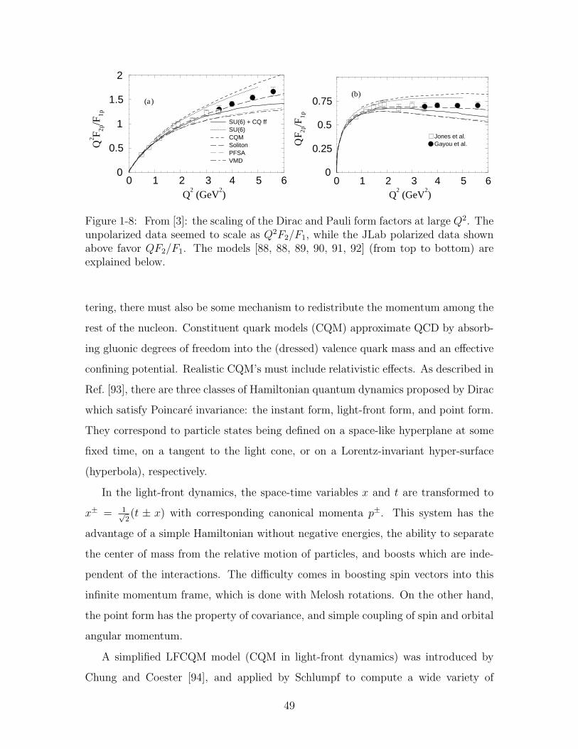
0 1 2 3 4 5 6Q

2 (GeV

2)

0

0.5

1

1.5

2

Q2 F 2p

/F1p

SU(6) + CQ ffSU(6) CQMSolitonPFSAVMD

(a )

0 1 2 3 4 5 6Q

2 (GeV

2)

0

0.25

0.5

0.75

QF 2p

/F1p

Jones et al.Gayou et al.

(b)

Figure 1-8: From [3]: the scaling of the Dirac and Pauli form factors at large Q2. Theunpolarized data seemed to scale as Q2F2/F1, while the JLab polarized data shownabove favor QF2/F1. The models [88, 88, 89, 90, 91, 92] (from top to bottom) areexplained below.

tering, there must also be some mechanism to redistribute the momentum among the

rest of the nucleon. Constituent quark models (CQM) approximate QCD by absorb-

ing gluonic degrees of freedom into the (dressed) valence quark mass and an effective

confining potential. Realistic CQM’s must include relativistic effects. As described in

Ref. [93], there are three classes of Hamiltonian quantum dynamics proposed by Dirac

which satisfy Poincare invariance: the instant form, light-front form, and point form.

They correspond to particle states being defined on a space-like hyperplane at some

fixed time, on a tangent to the light cone, or on a Lorentz-invariant hyper-surface

(hyperbola), respectively.

In the light-front dynamics, the space-time variables x and t are transformed to

x± = 1√2(t ± x) with corresponding canonical momenta p±. This system has the

advantage of a simple Hamiltonian without negative energies, the ability to separate

the center of mass from the relative motion of particles, and boosts which are inde-

pendent of the interactions. The difficulty comes in boosting spin vectors into this

infinite momentum frame, which is done with Melosh rotations. On the other hand,

the point form has the property of covariance, and simple coupling of spin and orbital

angular momentum.

A simplified LFCQM model (CQM in light-front dynamics) was introduced by

Chung and Coester [94], and applied by Schlumpf to compute a wide variety of

49

hadronic properties [95]. These models reproduced the form factor scaling of the

unpolarized data, failing to describe the polarized data. However, another calculation

by Frank, Jennings, and Miller [89] using the model of Schlumpf agrees well with

the complete polarized data set. Agreement was attributed to the limiting QF2/F1

dependence caused by imposing Poincare invariance [96], in potential violation of

the quark helicity conservation rule. Calculations by Cardarelli et al. [88] were also

carried out in light-front dynamics with a one-gluon exchange potential to study

SU(6) symmetry breaking. Their predictions for GE and GM with and without form

factors for the constituent quarks, also agree well with the polarized data.

A variant of the CQM model is the diquark model of Kroll et al. [97]. Two of the

constituent quarks are tightly-bound into a spin-0 or 1 diquark with a phenomeno-

logical form factor which allows the diquark to behave as free quarks at high Q2. The

electron may scatter from either the quark or diquark, and helicity-flip amplitudes

are generated by scattering from the spin-1 diquark. Ma, Qing, and Schmidt [98]

did calculations of a quark spectator-diquark model in light-front dynamics. Wa-

genbrunn et al. [91, 99] constructed a model in point form dynamics, following the

point form spectator approximation (PFSA) of Klink [100]. This model also uses a

Goldstone boson exchange potential, and is in good agreement with the form factors

from polarized data.

Another class of quark models based on the MIT Bag Model has three valence

quarks confined to a finite spherical well. Historically, these models were not able to

reproduce the static properties of the nucleon. Lu and Thomas [101] included a pion

field in the model to restore chiral symmetry and reproduce the low-Q2 properties of

the form factors with agreement up to Q2 < 1 (GeV/c)2. Miller applied the relativistic

dynamics of the quarks in the LFCQM to the pion cloud of the Cloudy Bag Model

(CBM) to create the so-called hybrid LFCBM [86]. The model describes all four

nucleon form factors using only four tunable parameters. It also has the correct low

Q2 behavior as required by chiral perturbation theory and therefore is very useful for

chiral extrapolations in lattice QCD (see Sec. 1.3.4). This model is one of the most

complete in terms of its incorporation of both meson and quark degrees of freedom,

50

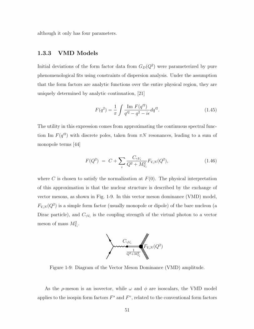
although it only has four parameters.

1.3.3 VMD Models

Initial deviations of the form factor data from GD(Q2) were parameterized by pure

phenomenological fits using constraints of dispersion analysis. Under the assumption

that the form factors are analytic functions over the entire physical region, they are

uniquely determined by analytic continuation, [21]

F (q2) =1

π

∫Im F (q′2)

q′2 − q2 − iεdq′2. (1.45)

The utility in this expression comes from approximating the continuous spectral func-

tion Im F (q′2) with discrete poles, taken from πN resonances, leading to a sum of

monopole terms [44]

F (Q2) = C +∑

i

CγVi

Q2 + M2Vi

FViN(Q2), (1.46)

where C is chosen to satisfy the normalization at F (0). The physical interpretation

of this approximation is that the nuclear structure is described by the exchange of

vector mesons, as shown in Fig. 1-9. In this vector meson dominance (VMD) model,

FViN(Q2) is a simple form factor (usually monopole or dipole) of the bare nucleon (a

Dirac particle), and CγViis the coupling strength of the virtual photon to a vector

meson of mass M2Vi

.

1Q2+M2

Vi

CγVi

FViN(Q2)

Figure 1-9: Diagram of the Vector Meson Dominance (VMD) amplitude.

As the ρ-meson is an isovector, while ω and φ are isoscalars, the VMD model

applies to the isospin form factors F s and F v, related to the conventional form factors

51

by

F p = F s + F v and F n = F s − F v. (1.47)

As F1 and F2, or GE and GM , cannot all satisfy Eq. 1.46, a choice must be made of

which pair to model, and the Dirac and Pauli form factors are preferred in the litera-

ture. Early data, e.g. [38, 21], were fit to the three resonance poles with considerable

improvement over the simple dipole fit. The dipole form comes naturally from two

resonances of similar mass and equal but opposite strengths, i.e. the derivative.

Later fits have included the width Γ = 150 MeV of the ρ meson through dispersion

relations and have include higher mass poles such as ω(1420) and ρ(1450). In addition

to the large width of ρ, there is a substantial non-resonance contribution to the

isovector dispersion spectrum between the two pion threshold and the ρ peak, which

is strong enough to affect the low Q2 behavior of the form factors and consequently

rp [25, 27].

Iachello et al. [102] fit all four nucleon form factors with a VMD model includ-

ing the width of ρ. They also modeled the bare nucleon with dipole, eikonal, and

monopole intrinsic form factors and included photon interaction with the bare nu-

cleon. Hohler et al. [12] calculated the ρ contribution using an analytic continuation

of πN scattering amplitudes and π form factor data instead of fitting the nucleon form

factor data with a single pole. They also introduced the isovector meson ρ′(1250 MeV)

much below its physical mass. This model was improved by Mergell et al. [27], updat-

ing the π form factors to account for ρ–ω mixing. They also matched the asymptotic

Q2 dependence to pQCD by constraining the free parameters with a set of super-

convergence relations.

The basic VMD model was also extended by Gari and Krumpelmann [103, 104]

with an additional term to guarantee the correct pQCD behavior at large Q2. Lomon

[92] updated this model with the width of ρ and the additional meson ρ′(1450). Later,

in order to explain the Hall A data, he extended the model [105] to include ω′(1419),

and excluded unpolarized data which was in conflict with the new polarized data to

get reasonable agreement. Hammer et al. [106] did a dispersion fit including form

52

factor data from the time-like region, and Kubis et al. [107] included vector mesons

in a fit using chiral perturbation theory, but neither of these calculations reproduce

the data at high Q2.

With the exception of Refs. [12] and [27] at low Q2, these VMD models are phe-

nomenological fits to the form factors with physics-inspired functions and constraints.

Therefore comparisons with new experimental data have limited meaning, since the

parameters must be returned to explain new data.

Holzwarth [90] investigated a topological soliton model of the nucleon based on

an effective nonlinear Lagrangian with mesonic degrees of freedom. Like the LFCBM

[86], this model was constructed as simple as possible from the essential elements

required to gain a physical understanding of the nuclear structure and make mean-

ingful comparisons with the data. The first of three important parts of this model

is a pionic soliton created from a standard Skyrme term in the Lagrangian. A single

vector meson pole ρ is coupled to both the isovector and isoscalar form factors with

an interpolation parameter λ ranging from 0 for pure Skyrme to 1 for pure VMD.

The third essential component is a relativistic boost to the Breit frame, which is also

important in constituent quark models. The resulting spectral function shows the

same behavior as Refs. [12, 27] between the two-pion threshold and ρ pole. This

model reproduces GpE and Gp

M including the form factor ratio very well, although it

underestimates GnE and overestimates Gn

M above Q2 = 1 (GeV/c)2. This model has

been updated [108] to include loop corrections.

1.3.4 Lattice QCD

Lattice QCD promises pure numerical calculations of the form factors straight from

the QCD Lagrangian without effective theories, models, or assumptions. Indeed the

hadron mass spectrum has been calculated on the lattice with success [109]. However,

these calculations are limited by computing power, and many approximations must be

made [110]. First, calculations are done on a discrete space-time with lattice spacing

a, and must be extrapolated to the continuum limit a → 0. This limit is under control

with improved actions such that O(a) errors are eliminated, and lattice spacings up

53

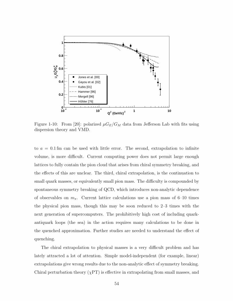
2 (GeV/c)2Q10

-210

-11 10

p M/G

p EG

pµ

0

0.2

0.4

0.6

0.8

1

Jones et al. [00]

Gayou et al. [02]

Kubis [01]

Hammer [96]

Mergell [96]

hler [76]oH

Figure 1-10: From [20]: polarized µGE/GM data from Jefferson Lab with fits usingdispersion theory and VMD.

to a = 0.1 fm can be used with little error. The second, extrapolation to infinite

volume, is more difficult. Current computing power does not permit large enough

lattices to fully contain the pion cloud that arises from chiral symmetry breaking, and

the effects of this are unclear. The third, chiral extrapolation, is the continuation to

small quark masses, or equivalently small pion mass. The difficulty is compounded by

spontaneous symmetry breaking of QCD, which introduces non-analytic dependence

of observables on mπ. Current lattice calculations use a pion mass of 6–10 times

the physical pion mass, though this may be soon reduced to 2–3 times with the

next generation of supercomputers. The prohibitively high cost of including quark-

antiquark loops (the sea) in the action requires many calculations to be done in

the quenched approximation. Further studies are needed to understand the effect of

quenching.

The chiral extrapolation to physical masses is a very difficult problem and has

lately attracted a lot of attention. Simple model-independent (for example, linear)

extrapolations give wrong results due to the non-analytic effect of symmetry breaking.

Chiral perturbation theory (χPT) is effective in extrapolating from small masses, and

54

captures the leading non-analytic behavior of QCD; however the radius of convergence

for χPT expansions is small compared to the calculated mass scale. Thus model-

dependent extrapolations are needed to respect the chiral symmetry for the current

range of m2π imposed by state-of-the-art lattice calculations. Such a model must have

a tunable m2π and satisfy the leading non-analytic (LNA) behavior and other formal

constraints of QCD. One suitable model, the CBM, is discussed below.

The QCDSF collaboration performed a quenched calculation [111] in 2003 of the

nucleon form factors up to Q2 ≈ 2 (GeV/c)2 at 3 different lattices from 163 × 32 to

323 × 48 and different spacings. They used O(a) improved Wilson fermions (clover)

with mass scale in the range 0.4 < m2π < 1.3 GeV2. Previous lattice QCD calculations

of the nucleon [112] had focused on the magnetic moments and charge radii.

Ashley et al. [113] have reported a chiral extrapolation of these new calculations

which satisfies the LNA behavior and other formal constraints of QCD. As the

calculations are not precise enough to distinguish between the Q2 dependence of

different models, they fit the calculations to isoscalar and isovector dipole form factors

with the mass scale Λ a continuous function of m2π. In the case of the isoscalar form

factors, with no LNA behavior, they did linear extrapolations of Λ(m2π), while for the

isovector case the functional form of the extrapolation was inspired from studies of

the CBM.

Thomas and collaborators [114] have successfully used the light-front cloudy bag

model (LFCBM) [86] for chiral extrapolation. The model was constructed to both

respect chiral symmetry through the pion cloud and Lorentz invariance through the

use of light-front dynamics. It was able to reproduce the m2π and also Q2 dependence of

the lattice calculations, and also has the proper LNA behavior QCD. They found that

the pion cloud was not important at the mass range of the lattice calculations, but very

significant near the chiral limit. Their extrapolation agrees well with experimental

form factors, and through a severe extrapolation of Q2 > 2 (GeV/c)2, they predict

that µGE/GM crosses 0 at about Q2 ≈ 6 (GeV/c)2. While these results are promising,

there is clearly a need to test extrapolation with other suitable models to investigate

the model dependence.

55

The Lattice Hadron Physics Collaboration (LHPC) has performed an unquenched

calculation [115] of the hadron form-factors using a hybrid scheme with staggered sea

quarks and domain wall valence quarks. Their calculation was done on a 203 × 64

lattice with spacing a = 0.125 fm using a PC cluster at JLab. The results were in

agreement with the QCDSF calculation.

Rapid progress in lattice QCD has been made in the use of sophisticated actions,

extrapolation techniques, and also in sheer computing power. In the near future

Lattice QCD calculations will progress to the point where they can be tested with

precision form factor measurements in the Q2 region of the current experiment.

1.4 Current Experiment

We have measured double-spin asymmetries of the elastic ~p(~e, e′p) channel at 0.15 <

Q2 < 0.65 (GeV/c)2. These high-precision asymmetries have been used to extract the

form factor ratio µGE/GM of the proton for the first time from this reaction. The

only prior measurement of this asymmetry [49] was performed at the single point

Q2 = 0.765 (GeV/c)2 and with large statistical uncertainty. The kinematics of that

experiment maximized the asymmetry, but minimized its sensitivity to µGE/GM .

However, the sign of GE/GM was determined to be positive.

1.4.1 Experimental Overview

From Eq. 1.27, the experimental double-spin asymmetry for elastic ~p(~e, e′p) scattering

is the product of the beam and target polarization, Pb and Pt, and the ratio of the

polarized over the unpolarized hydrogen elastic cross section [6]

Aexp = PbPtzGM

2 + xGEGM

τGM2 + εGE

2 , (1.48)

where τ = Q2/4M2, and ε = 1/(1 + 2(1+τ) tan2 θ2) is the longitudinal polarization of

the virtual photon. The terms including the kinematic factors z and x are proportional

to the longitudinal and transverse components of the proton polarization z∗ and x∗

56

with respect to the momentum transfer, q.

By simultaneously measuring the asymmetry for two different spin orientations

at fixed Q2, one can form a super-ratio RA of the asymmetries in which the beam

and target polarization and the unpolarized cross section cancel. Given a symmet-

ric detector, both asymmetries can be measured at the same time by orienting the

target spin at the angle β = 45 to the left of the beam, so that the asymmetry AL

(AR) for electrons scattering into the left (right) sector is predominantly transverse

(longitudinal). The super-ratio of these two independent asymmetries is

RA ≡ AL

AR

=zL + xLR

zR + xRR. (1.49)

The form factor ratio R = GE/GM can be extracted from the solution of Eq. 1.49.

From the two asymmetries AL and AR at each Q2 point, one may also extract

the product of beam and target polarization P = PbPt. A comparison of the values

of P at each Q2 point gives a measure of data quality. By constraining each P to

be the same, one may effectively apply extra statistics toward the form factor ratio,

the quantity of physical interest. By using some model of µGE/GM at the lowest Q2

point to fix the polarization, one may also extract µGE/GM from a single asymmetry

measurement, although with lower statistical precision. The experimental setup and

detailed analysis are described in the following chapters.

1.4.2 Physics Impact

The purpose of this experiment was to map out the form factors in the low-Q2 region

of the pion cloud. These data may be used to test the various form factor models

which are applicable in this region, or may be used to tune their low Q2 dependence.

Particularly important will be the test of ab-initio lattice QCD calculations once

they are precise enough for comparison. Precise measurements of GE and GM are

also important as physics input for parity violating experiments on the proton [76,

116, 117, 118, 77].

In light of the discrepancy between unpolarized extractions of µGE/GM and the

57

FPP results from JLab, this experiment is an independent verification of the validity

of form factor extraction from the polarized asymmetry. Although formally both

experiments measure the same observable, the systematic uncertainties from each

method are very different. The FPP analysis hinges on a careful determination of the

spin precession of the recoil proton through the optics of the spectrometer, while our

data are most sensitive to the determination of the momentum transfer ~q and the spin

angle of the polarized target. There are high statistics FPP data from MIT-Bates,

Mainz, and JLab in the region of this measurement allowing for a rigorous cross-check

of the FPP results at low Q2.

This experiment also includes data up to Q2 = 0.9 (GeV/c)2 from the backward

angle TOFs, which are not included in this thesis. This is at the threshold where the

JLab data depart from µGE/GM ≈ 1 scaling. With data from backward angle TOFs,

not included in this thesis, the BLAST measurement of µGE/GM extends to Q2 =

0.9 (GeV/c)2, high enough in Q2 that the JLab measurement of µGE/GM at the same

value of Q2 has dropped significantly below 1. There is a deferred proposal to measure

µGE/GM from elastic ~p(~e, e′p) at JLab in Hall C [119]. Just as FPP measurements of

µGE/GM were pioneered at MIT-Bates and then repeated at JLab, our experiment

may provide valuable input into future polarized target JLab measurement, which

can be done to much higher Q2. Finally, as higher order radiative corrections are

developed to reconcile the polarized and unpolarized data, our measurements at low

Q2 can constrain the theory at the point where the corrections are small.

58

Chapter 2

Experimental Setup

The measurement of µGE/GM was performed in the South Hall Ring (SHR) of the

Bates Linear Accelerator Center, using the Atomic Beam Source (ABS) and the

BLAST detector package. These three key components (the polarized beam, polarized

target, and detectors) are described below.

2.1 Polarized Beam

2.1.1 Polarized Source

The polarized electron source [120] uses a strained GaAs crystal photo-cathode illumi-

nated by a circularly polarized laser, similar to polarized sources at JLab and SLAC.

The strain in the GaAs crystal removes the degeneracy in energy levels, increasing the

maximum polarization from 50% to 100% at the expense of low quantum efficiency.

In practice, the polarization is limited to about 80% by electron depolarization during

diffusing to the surface and by strain relaxation. Therefore the active layer must be

very thin, on the order of 100 nm. The work function of the crystal is decreased by

mono-layer coating of cesium, which must be restored about once a week.

The high polarization is gained at the expense of low quantum efficiency, about

0.1%. Thus it is necessary to illuminate the photocathode with an intense laser beam.

The Bates polarized source uses a commercially available 150 W fiber-coupled diode

59

array laser system at the fixed wavelength of 808 nm. Special GaAs crystals optimized

for this higher wavelength have been grown by Bandwidth Semiconductor and a group

in St. Petersburg, and crystals from both groups generate a polarization in excess of

75%. Also a pre-prebuncher was installed to increased the electron capture efficiency

from 30% to 50%. With these improvements, the source was able to inject 6 mA into

the accelerator.

The laser beam is passed through a linear polarizer and a λ/4 wave-plate before

being focused on the photo-cathode. The beam helicity is reversed by the mechanical

insertion of a λ/2 wave-plate into the beam. This is controlled automatically by the

beam-fill software. A Wien filter in the polarized source selects the spin direction

such that after acceleration, recirculation, and transport, the beam is longitudinally

polarized in the region of the internal target.

The beam polarization at the source is periodically measured with a transmis-

sion polarimeter [121], consisting of a bremsstrahlung radiator followed by a 6′′ steel

core absorber magnet. The longitudinal polarization of the beam is transfered to

the bremsstrahlung photons, which are monitored before and after the absorber with

scintillators. The beam polarization is extracted from the asymmetry in the helic-

ity dependent transmission of bremsstrahlung photons through the absorber. The

transmission polarimeter was cross-calibrated against the S-Line Møller polarimeter

during the SAMPLE experiment [122].

2.1.2 Storage Ring

The polarized electrons are accelerated up to 1 GeV by the linear accelerator and

injected into the South Hall Ring (SHR). The linac has 190 m of RF cavities with

a duty factor of 1%, capable of energies up to 540 MeV. A recirculator transports

the beam back to the beginning of the accelerator for a second pass through the RF

cavities, nearly doubling the beam energy. Figure 2-1 shows a plan of the MIT-Bates

Linear Accelerator Facility with the accelerator, SHR, and experimental halls.

The SHR [123] may either be operated in pulse stretcher mode for external targets

or as a storage ring for internal targets. The ring specifications during this experiment

60

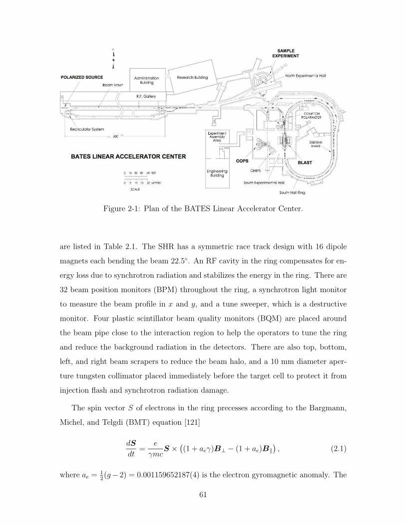
Figure 2-1: Plan of the BATES Linear Accelerator Center.

are listed in Table 2.1. The SHR has a symmetric race track design with 16 dipole

magnets each bending the beam 22.5. An RF cavity in the ring compensates for en-

ergy loss due to synchrotron radiation and stabilizes the energy in the ring. There are

32 beam position monitors (BPM) throughout the ring, a synchrotron light monitor

to measure the beam profile in x and y, and a tune sweeper, which is a destructive

monitor. Four plastic scintillator beam quality monitors (BQM) are placed around

the beam pipe close to the interaction region to help the operators to tune the ring

and reduce the background radiation in the detectors. There are also top, bottom,

left, and right beam scrapers to reduce the beam halo, and a 10 mm diameter aper-

ture tungsten collimator placed immediately before the target cell to protect it from

injection flash and synchrotron radiation damage.

The spin vector S of electrons in the ring precesses according to the Bargmann,

Michel, and Telgdi (BMT) equation [121]

dS

dt=

e

γmcS ×

((1 + aeγ)B⊥ − (1 + ae)B‖

), (2.1)

where ae = 12(g− 2) = 0.001159652187(4) is the electron gyromagnetic anomaly. The

61

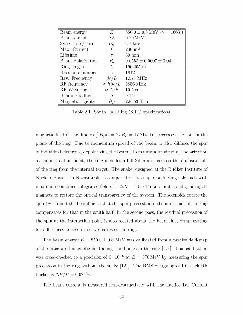
Beam energy E 850.0± 0.8 MeV (γ = 1663.)Beam spread ∆E 0.20 MeVSync. Loss/Turn U0 5.1 keVMax. Current I 230 mALifetime τ 30 minBeam Polarization Pb 0.6558± 0.0007± 0.04Ring length L 190.205 mHarmonic number h 1812Rev. Frequency βc/L 1.577 MHzRF frequency ≈ hβc/L 2856 MHzRF Wavelength ≈ L/h 10.5 cmBending radius ρ 9.144Magnetic rigidity Bρ 2.8353 T m

Table 2.1: South Hall Ring (SHR) specifications.

magnetic field of the dipoles∫

Byds = 2πBρ = 17.814 Tm precesses the spin in the

plane of the ring. Due to momentum spread of the beam, it also diffuses the spin

of individual electrons, depolarizing the beam. To maintain longitudinal polarization

at the interaction point, the ring includes a full Siberian snake on the opposite side

of the ring from the internal target. The snake, designed at the Budker Institute of

Nuclear Physics in Novosibirsk, is composed of two superconducting solenoids with

maximum combined integrated field of∫

dsB‖ = 10.5 Tm and additional quadrupole

magnets to restore the optical transparency of the system. The solenoids rotate the

spin 180 about the beamline so that the spin precession in the north half of the ring

compensates for that in the south half. In the second pass, the residual precession of

the spin at the interaction point is also rotated about the beam line, compensating

for differences between the two halves of the ring.

The beam energy E = 850.0 ± 0.8 MeV was calibrated from a precise field-map

of the integrated magnetic field along the dipoles in the ring [124]. This calibration

was cross-checked to a precision of 6×10−6 at E = 370 MeV by measuring the spin

precession in the ring without the snake [121]. The RMS energy spread in each RF

bucket is ∆E/E = 0.024%.

The beam current is measured non-destructively with the Lattice DC Current

62

Transformer (LDCCT), a parametric current transformer developed by Unser [125].

The technology used to measure DC currents is a saturatable core primary winding

around the beam with a nonlinear magnetic response to current. It is coupled to a

secondary winding which is driven with a fixed signal. Pickup electronics measure

the second harmonic generated by the nonlinear response, which is proportional to

the absolute beam current passing through the coil with absolute accuracy of 0.05%.

The LDCCT signal is output to both a 16 bit ADC, which is read as an EPICS

variable (Sec. 2.4.2), and to a voltage-to-frequency (V2F) converter. The number of

oscillations of the V2F, proportional to the integrated beam current, are counted in

two scaler channels, DCCT and BDCCT. The latter is gated by the trigger supervisor

inhibit signal when the data acquisition is busy, when the target is in a transition

between well-defined states, or when the high voltage trips or is put to standby. Thus

the BDCCT scaler measures the actual charge passing through the target while the

experiment is taking data, which eliminates the need to be correct the yields for

deadtime. This is important in the case where correctable false asymmetries prevent

applying an overall deadtime dilution factor to the physics asymmetry. The DAQ

deadtime fraction, 1− BDCCT/DCCT, is determined from these two scalers.

The LDCCT is monitored regularly with current injected into a calibration loop

and measured with an ammeter with 1 pA resolution, also output to EPICS. The

beam scalers were calibrated during fake runs in which the beam was turned off and

currents ranging from 0–200 mA in steps of 5 mA were injected in the calibration

loop. The calibration from this data, good to 0.5% for currents over 20 mA, is

Q =(2.90027 + 3.01409×10−4 S + 6.18094×10−10 S2

)mC, (2.2)

where S is the DCCT or BDCCT scalers value after a pedestal subtraction of 2400

counts. Currents up to 300 mA have been stored in the ring, but to prevent radiation

damage to windows and to the target cell, our experiment was limited to 195 mA in

the ring until the last few days, when it was increased to 225 mA.

63

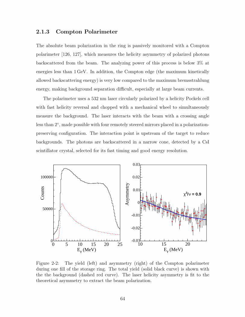
2.1.3 Compton Polarimeter

The absolute beam polarization in the ring is passively monitored with a Compton

polarimeter [126, 127], which measures the helicity asymmetry of polarized photons

backscattered from the beam. The analyzing power of this process is below 3% at

energies less than 1 GeV. In addition, the Compton edge (the maximum kinetically

allowed backscattering energy) is very low compared to the maximum bremsstrahlung

energy, making background separation difficult, especially at large beam currents.

The polarimeter uses a 532 nm laser circularly polarized by a helicity Pockels cell

with fast helicity reversal and chopped with a mechanical wheel to simultaneously

measure the background. The laser interacts with the beam with a crossing angle

less than 2, made possible with four remotely steered mirrors placed in a polarization-

preserving configuration. The interaction point is upstream of the target to reduce

backgrounds. The photons are backscattered in a narrow cone, detected by a CsI

scintillator crystal, selected for its fast timing and good energy resolution.

(MeV)γE0 5 10 15 20 25

C

ount

s

0

50000

100000

(MeV)γE10 15 20

Asy

mm

etry

-0.03

-0.02

-0.01

0

0.01

0.02

0.03

= 0.9ν/2χ

Figure 2-2: The yield (left) and asymmetry (right) of the Compton polarimeterduring one fill of the storage ring. The total yield (solid black curve) is shown withthe the background (dashed red curve). The laser helicity asymmetry is fit to thetheoretical asymmetry to extract the beam polarization.

64

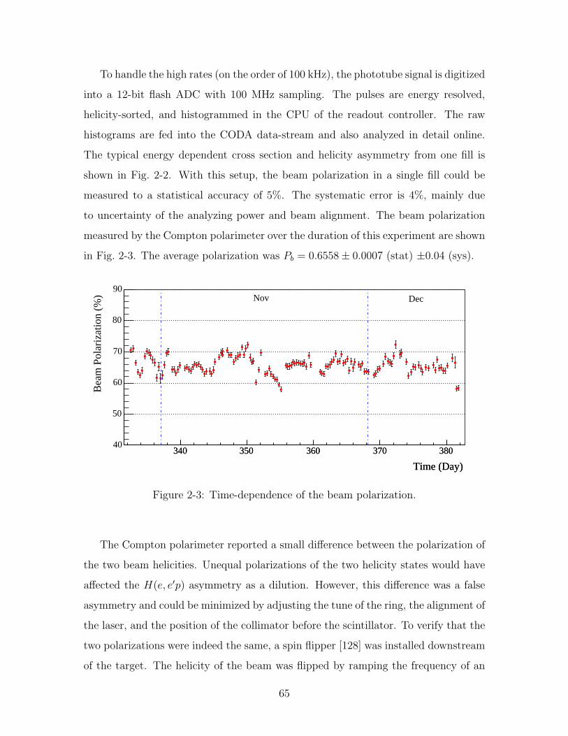
To handle the high rates (on the order of 100 kHz), the phototube signal is digitized

into a 12-bit flash ADC with 100 MHz sampling. The pulses are energy resolved,

helicity-sorted, and histogrammed in the CPU of the readout controller. The raw

histograms are fed into the CODA data-stream and also analyzed in detail online.

The typical energy dependent cross section and helicity asymmetry from one fill is

shown in Fig. 2-2. With this setup, the beam polarization in a single fill could be

measured to a statistical accuracy of 5%. The systematic error is 4%, mainly due

to uncertainty of the analyzing power and beam alignment. The beam polarization

measured by the Compton polarimeter over the duration of this experiment are shown

in Fig. 2-3. The average polarization was Pb = 0.6558± 0.0007 (stat) ±0.04 (sys).

Time (Day)

340 350 360 370 380

Time (Day)

340 350 360 370 380

Bea

m P

olar

izat

ion

(%)

40

50

60

70

80

90Nov Dec

Figure 2-3: Time-dependence of the beam polarization.

The Compton polarimeter reported a small difference between the polarization of

the two beam helicities. Unequal polarizations of the two helicity states would have

affected the H(e, e′p) asymmetry as a dilution. However, this difference was a false

asymmetry and could be minimized by adjusting the tune of the ring, the alignment of

the laser, and the position of the collimator before the scintillator. To verify that the

two polarizations were indeed the same, a spin flipper [128] was installed downstream

of the target. The helicity of the beam was flipped by ramping the frequency of an

65

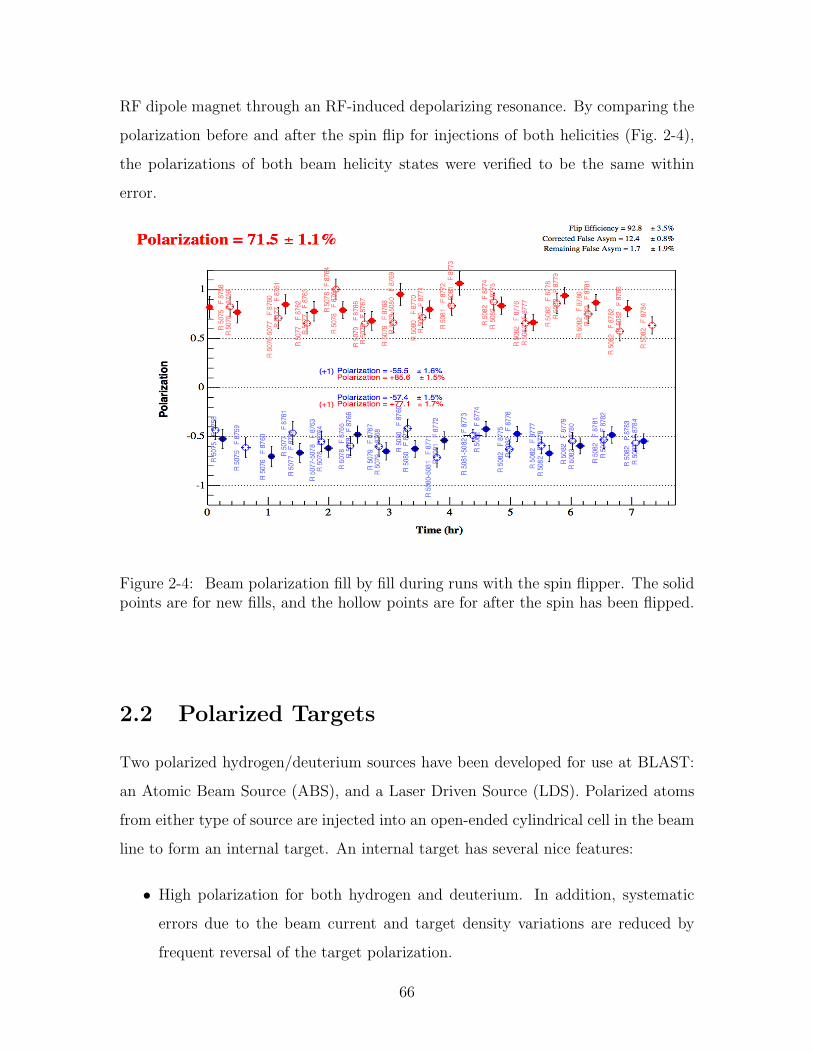
RF dipole magnet through an RF-induced depolarizing resonance. By comparing the

polarization before and after the spin flip for injections of both helicities (Fig. 2-4),

the polarizations of both beam helicity states were verified to be the same within

error.

Figure 2-4: Beam polarization fill by fill during runs with the spin flipper. The solidpoints are for new fills, and the hollow points are for after the spin has been flipped.

2.2 Polarized Targets

Two polarized hydrogen/deuterium sources have been developed for use at BLAST:

an Atomic Beam Source (ABS), and a Laser Driven Source (LDS). Polarized atoms

from either type of source are injected into an open-ended cylindrical cell in the beam

line to form an internal target. An internal target has several nice features:

• High polarization for both hydrogen and deuterium. In addition, systematic

errors due to the beam current and target density variations are reduced by

frequent reversal of the target polarization.

66

• Low backgrounds as the target is a pure atomic species. Also, there are no

beam entrance or exit windows.

However, the thickness of internal targets is limited and must be compensated by an

intense electron beam and a large acceptance spectrometer in order to attain practical

event rates.

The ABS is based on standard technology and has been used in numerous nuclear

and high energy physics laboratories, including NIKHEF (AmPS), DESY (HERMES),

IUCF, BNL (RHIC), and COSY. An intense atomic beam is formed of dissociated

hydrogen/deuterium directed through a cryogenic nozzle, skimmer, and collimator.

The atoms are nuclear polarized passively by a series of Stern-Gerlach type spin filters

and RF transitions before being injected into the storage cell. This source produces

very high target nuclear polarization Pt, but with limited target thickness ρ.

The LDS is a novel source which actively polarizes hydrogen/deuterium atoms via

the transfer of angular momentum from a circularly polarized laser. There is no need

for spin filtering and all of the gas passes through to the target cell. As a result, the

polarization is lower, but the target thickness is substantially greater, allowing for a

higher overall figure of merit. An LDS was used at IUCF for polarized pd scattering

[129]. Although not as common for polarized hydrogen/deuterium targets, optical

pumping is the standard method of polarizing the noble gasses He and Xe.

A comparison of the performance of both types of targets is shown in Table 2.2.

The figure of merit (FOM) F = ρ·P 2t is a measure of the statistical precision obtained

from a given experimental run time. Only the atomic polarization Pe was measured

in our LDS, but the nuclear polarization Pt is related by

Pt =Pefα

fα +√

2(1− fα)(2.3)

under the assumption of spin temperature equilibrium (STE), which has been estab-

lished by experiments at Erlangen [130] and IUCF [129]. We assume the worst case,

that hydrogen atoms are completely depolarized after recombining into molecules.

67

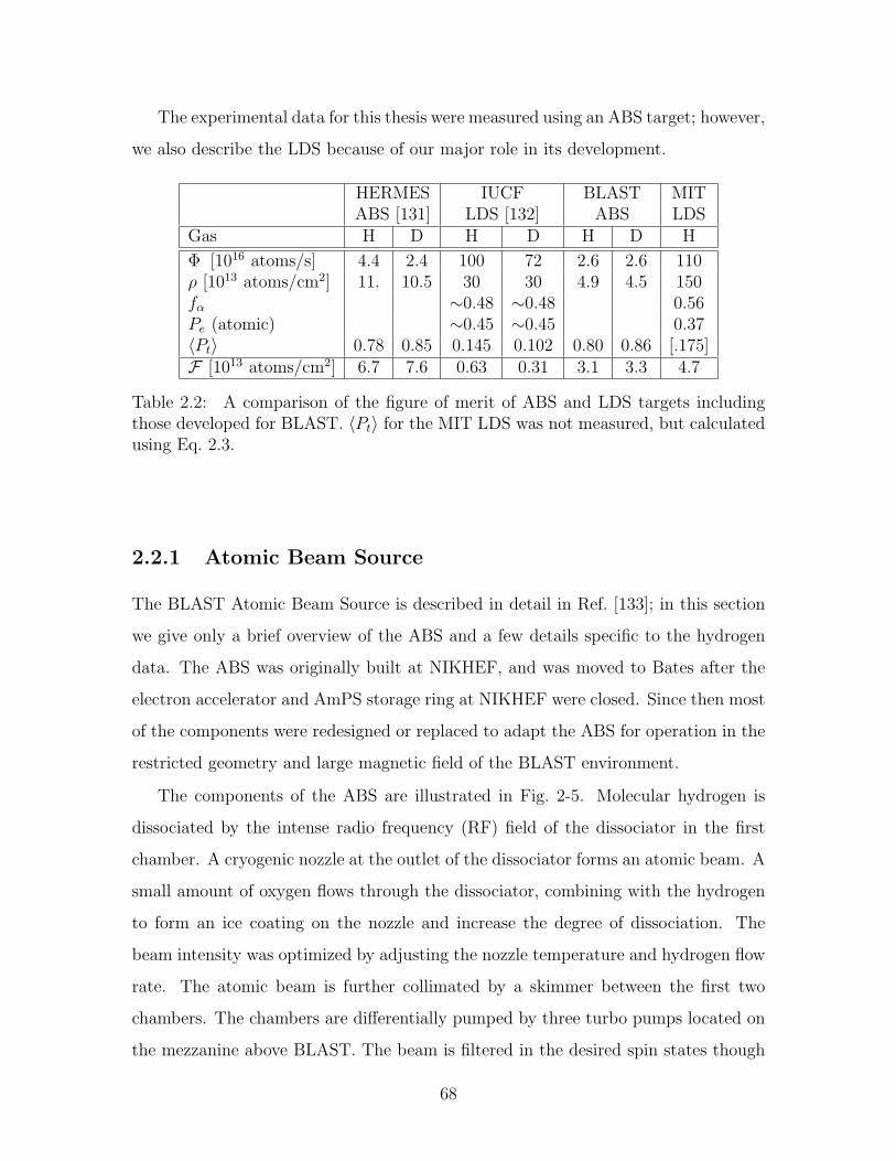
The experimental data for this thesis were measured using an ABS target; however,

we also describe the LDS because of our major role in its development.

HERMES IUCF BLAST MITABS [131] LDS [132] ABS LDS

Gas H D H D H D H

Φ [1016 atoms/s] 4.4 2.4 100 72 2.6 2.6 110ρ [1013 atoms/cm2] 11. 10.5 30 30 4.9 4.5 150fα ∼0.48 ∼0.48 0.56Pe (atomic) ∼0.45 ∼0.45 0.37〈Pt〉 0.78 0.85 0.145 0.102 0.80 0.86 [.175]F [1013 atoms/cm2] 6.7 7.6 0.63 0.31 3.1 3.3 4.7

Table 2.2: A comparison of the figure of merit of ABS and LDS targets includingthose developed for BLAST. 〈Pt〉 for the MIT LDS was not measured, but calculatedusing Eq. 2.3.

2.2.1 Atomic Beam Source

The BLAST Atomic Beam Source is described in detail in Ref. [133]; in this section

we give only a brief overview of the ABS and a few details specific to the hydrogen

data. The ABS was originally built at NIKHEF, and was moved to Bates after the

electron accelerator and AmPS storage ring at NIKHEF were closed. Since then most

of the components were redesigned or replaced to adapt the ABS for operation in the

restricted geometry and large magnetic field of the BLAST environment.

The components of the ABS are illustrated in Fig. 2-5. Molecular hydrogen is

dissociated by the intense radio frequency (RF) field of the dissociator in the first

chamber. A cryogenic nozzle at the outlet of the dissociator forms an atomic beam. A

small amount of oxygen flows through the dissociator, combining with the hydrogen

to form an ice coating on the nozzle and increase the degree of dissociation. The

beam intensity was optimized by adjusting the nozzle temperature and hydrogen flow

rate. The atomic beam is further collimated by a skimmer between the first two

chambers. The chambers are differentially pumped by three turbo pumps located on

the mezzanine above BLAST. The beam is filtered in the desired spin states though

68

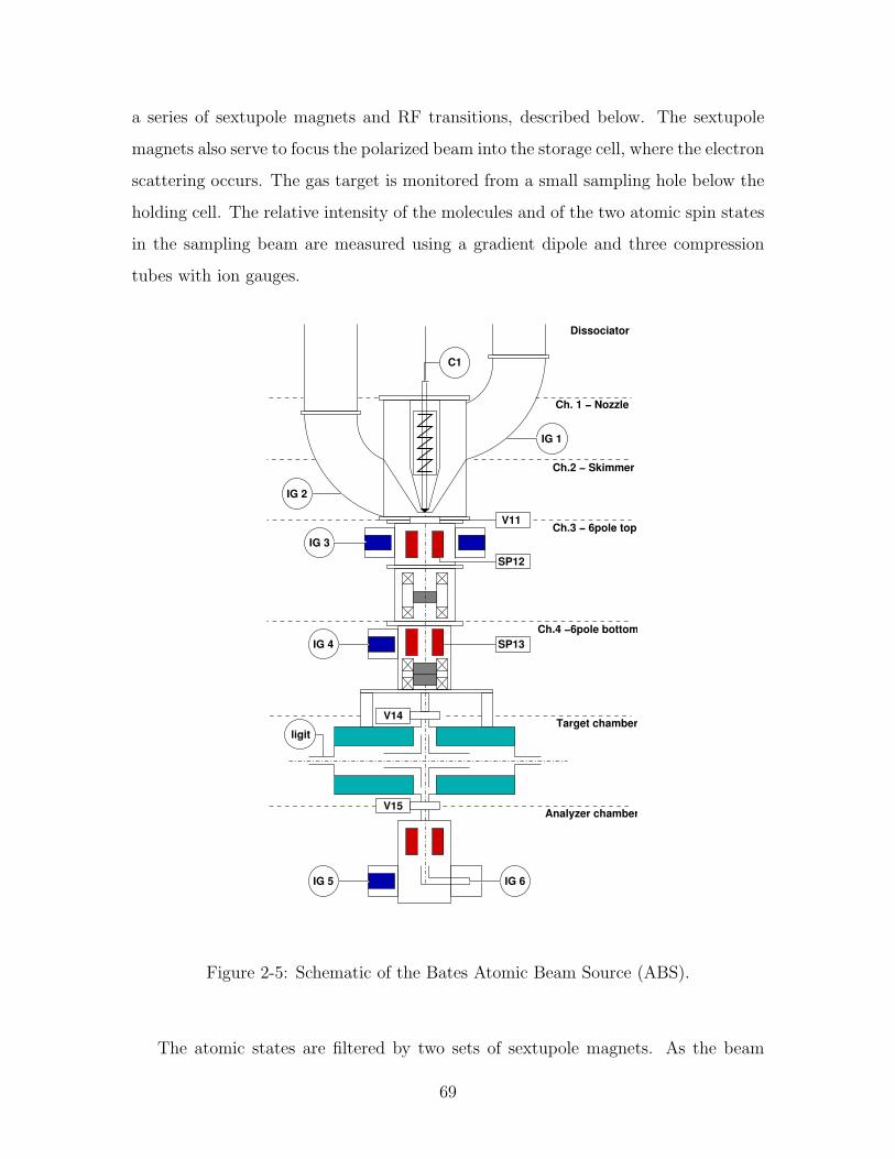
a series of sextupole magnets and RF transitions, described below. The sextupole

magnets also serve to focus the polarized beam into the storage cell, where the electron

scattering occurs. The gas target is monitored from a small sampling hole below the

holding cell. The relative intensity of the molecules and of the two atomic spin states

in the sampling beam are measured using a gradient dipole and three compression

tubes with ion gauges.

IG 1

V14

V15

IG 3

IG 4

IG 5 IG 6

C1

V11

SP12

SP13

Ch.3 − 6pole top

ligitTarget chamber

Analyzer chamber

Ch.4 −6pole bottom

Ch.2 − Skimmer

IG 2

Ch. 1 − Nozzle

Dissociator

Figure 2-5: Schematic of the Bates Atomic Beam Source (ABS).

The atomic states are filtered by two sets of sextupole magnets. As the beam

69

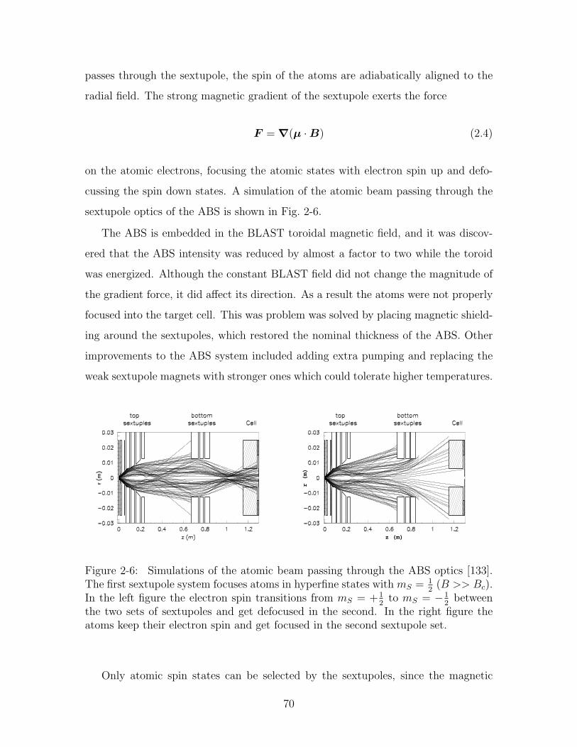
passes through the sextupole, the spin of the atoms are adiabatically aligned to the

radial field. The strong magnetic gradient of the sextupole exerts the force

F = ∇(µ ·B) (2.4)

on the atomic electrons, focusing the atomic states with electron spin up and defo-

cussing the spin down states. A simulation of the atomic beam passing through the

sextupole optics of the ABS is shown in Fig. 2-6.

The ABS is embedded in the BLAST toroidal magnetic field, and it was discov-

ered that the ABS intensity was reduced by almost a factor to two while the toroid

was energized. Although the constant BLAST field did not change the magnitude of

the gradient force, it did affect its direction. As a result the atoms were not properly

focused into the target cell. This was problem was solved by placing magnetic shield-

ing around the sextupoles, which restored the nominal thickness of the ABS. Other

improvements to the ABS system included adding extra pumping and replacing the

weak sextupole magnets with stronger ones which could tolerate higher temperatures.

z (m)

r (m)

Figure 2-6: Simulations of the atomic beam passing through the ABS optics [133].The first sextupole system focuses atoms in hyperfine states with mS = 1

2(B >> Bc).

In the left figure the electron spin transitions from mS = +12

to mS = −12

betweenthe two sets of sextupoles and get defocused in the second. In the right figure theatoms keep their electron spin and get focused in the second sextupole set.

Only atomic spin states can be selected by the sextupoles, since the magnetic

70

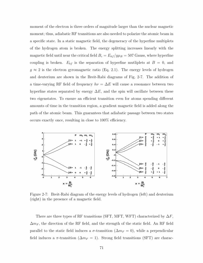
moment of the electron is three orders of magnitude larger than the nuclear magnetic

moment; thus, adiabatic RF transitions are also needed to polarize the atomic beam in

a specific state. In a static magnetic field, the degeneracy of the hyperfine multiplets

of the hydrogen atom is broken. The energy splitting increases linearly with the

magnetic field until near the critical field Bc = Ehf/gµB = 507 Gauss, where hyperfine

coupling is broken. Ehf is the separation of hyperfine mutliplets at B = 0, and

g ≈ 2 is the electron gyromagnetic ratio (Eq. 2.1). The energy levels of hydrogen

and deuterium are shown in the Breit-Rabi diagrams of Fig. 2-7. The addition of

a time-varying RF field of frequency hν = ∆E will cause a resonance between two

hyperfine states separated by energy ∆E, and the spin will oscillate between these

two eigenstates. To ensure an efficient transition even for atoms spending different

amounts of time in the transition region, a gradient magnetic field is added along the

path of the atomic beam. This guarantees that adiabatic passage between two states

occurs exactly once, resulting in close to 100% efficiency.

0 1 2 3 4 5 6

-3

-2

-1

0

1

2

3

4F Fm Im Sm

|1> 1 +121+

21+

|2> 1 021-

21+

|3> 1 -1 21- 2

1-

|4> 0 021+

21-

cHB

B x =

(GHz

)HFH ν

0 1 2 3 4 5 6 7-0.8

-0.6

-0.4

-0.2

-0

0.2

0.4

0.6

0.8 F Fm Im Sm|1>

23

23+ + 1

21+

|2> 23

21+ 0 2

1+

|3>23

21- - 1

21+

|4>23

23- - 1

21-

|5> 21

21- 0 2

1-

|6>21

21+ + 1

21-

cDB

B x =

(GHz

)HFD ν

Figure 2-7: Breit-Rabi diagram of the energy levels of hydrogen (left) and deuterium(right) in the presence of a magnetic field.

There are three types of RF transitions (SFT, MFT, WFT) characterized by ∆F ,

∆mF , the direction of the RF field, and the strength of the static field. An RF field

parallel to the static field induces a σ-transition (∆mF = 0), while a perpendicular

field induces a π-transition (∆mF = 1). Strong field transitions (SFT) are charac-

71

terized by ∆F = 1, while medium and weak field transitions (MFT, WFT) exchange

states among the same hyperfine multiplet (∆F = 0). Only the MFT and WFT are

used to polarize hydrogen.

In strong magnetic fields where B Bc, the nuclear and electronic spin states

decouple, and the nuclear spin is a good quantum number: mI = 12

for states |1〉, |4〉,

and mI = −12

for states |2〉, |3〉. However if the holding field is not strong enough,

there is a residual hyperfine interaction which lowers the polarization of states |2〉

and |4〉. Therefore, our experiment was carried out using single state injection of the

pure states |1〉 and |3〉, which do not mix via the hyperfine interaction. State |3〉 is

prepared through the series of sextupole filters and RF transitionsn1

n2

n3

n4

6−pol−→

n1

n2

0

0

MFT π23−→

n1

0

n2

0

6−pol−→

n1

0

0

0

WFT π13−→

0

0

n1

0

, (2.5)

where ni are the initial population density of each state. For state |1〉 injection, the

last transition (π13) is omitted; this is the only difference between the preparation of

the two target polarization states. The WFT requires a lower gradient field, improving

the transition efficiency; therefore asymmetry in the intensity and polarization of the

two target states is expected to be small. Indeed this was observed in measurements

of the target false asymmetry (Sec. 3.4.6).

The atomic beam is injected into a cylindrical storage cell, which increases the

target thickness in comparison to a pure atomic beam. The inlet of the storage cell is

also a cylinder with approximately the same conductance as either half of the storage

cell. The cell is cooled to about 100 K. The experiment was commissioned with a

40 cm long storage cell, while the the production data were taken with a 60 cm cell.

There are transverse and longitudinal coils wound around iron yokes above and

below the scattering chamber to create a holding field of arbitrary direction. The spin

orientation of the target is adjusted by varying the current in each set of coils. Data

were taken at two spin angles, β = 47.2 and β = 31.4. After the production run, the

72

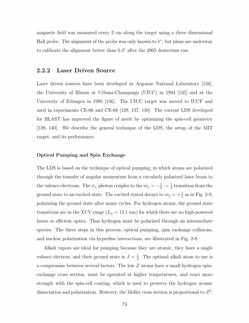
magnetic field was measured every 2 cm along the target using a three dimensional

Hall probe. The alignment of the probe was only known to 1, but plans are underway

to calibrate the alignment better than 0.3 after the 2005 deuterium run.

2.2.2 Laser Driven Source

Laser driven sources have been developed at Argonne National Laboratory [134],

the University of Illinois at Urbana-Champaign (UIUC) in 1994 [135] and at the

University of Erlangen in 1995 [136]. The UIUC target was moved to IUCF and

used in experiments CE-66 and CE-68 [129, 137, 138]. The current LDS developed

for BLAST has improved the figure of merit by optimizing the spin-cell geometry

[139, 140]. We describe the general technique of the LDS, the setup of the MIT

target, and its performance.

Optical Pumping and Spin Exchange

The LDS is based on the technique of optical pumping, in which atoms are polarized

through the transfer of angular momentum from a circularly polarized laser beam to

the valence electrons. The σ+ photon couples to the mj = −12→ 1

2transition from the

ground state to an excited state. The excited stated decays to mj = +12

as in Fig. 2-9,

polarizing the ground state after many cycles. For hydrogen atoms, the ground state

transitions are in the XUV range (Lα = 12.1 nm) for which there are no high-powered

lasers or efficient optics. Thus hydrogen must be polarized through an intermediate

species. The three steps in this process, optical pumping, spin exchange collisions,

and nuclear polarization via hyperfine interactions, are illustrated in Fig. 2-8.

Alkali vapors are ideal for pumping because they are atomic, they have a single

valence electron, and their ground state is J = 12. The optimal alkali atom to use is

a compromise between several factors. The low Z atoms have a small hydrogen spin-

exchange cross section, must be operated at higher temperatures, and react more

strongly with the spin-cell coating, which is used to preserve the hydrogen atomic

dissociation and polarization. However, the Møller cross section is proportional to Z2.

73

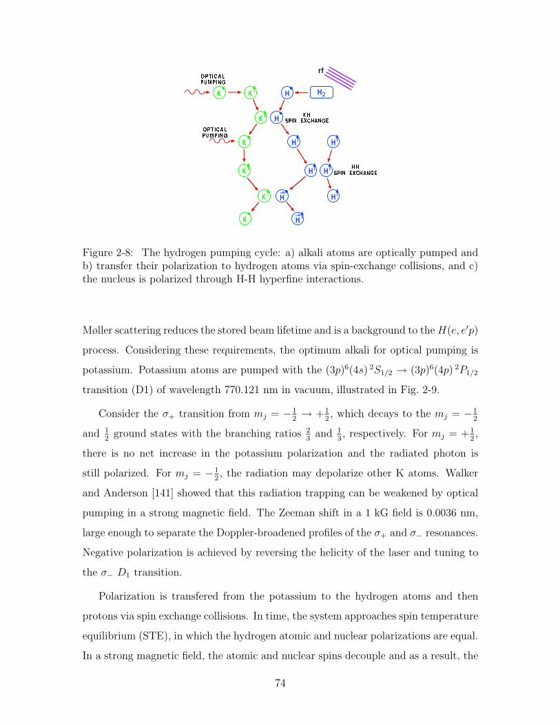
K K

K

K

K

K

K

U

U

K

Figure 2-8: The hydrogen pumping cycle: a) alkali atoms are optically pumped andb) transfer their polarization to hydrogen atoms via spin-exchange collisions, and c)the nucleus is polarized through H-H hyperfine interactions.

Møller scattering reduces the stored beam lifetime and is a background to the H(e, e′p)

process. Considering these requirements, the optimum alkali for optical pumping is

potassium. Potassium atoms are pumped with the (3p)6(4s) 2S1/2 → (3p)6(4p) 2P1/2

transition (D1) of wavelength 770.121 nm in vacuum, illustrated in Fig. 2-9.

Consider the σ+ transition from mj = −12→ +1

2, which decays to the mj = −1

2

and 12

ground states with the branching ratios 23

and 13, respectively. For mj = +1

2,

there is no net increase in the potassium polarization and the radiated photon is

still polarized. For mj = −12, the radiation may depolarize other K atoms. Walker

and Anderson [141] showed that this radiation trapping can be weakened by optical

pumping in a strong magnetic field. The Zeeman shift in a 1 kG field is 0.0036 nm,

large enough to separate the Doppler-broadened profiles of the σ+ and σ− resonances.

Negative polarization is achieved by reversing the helicity of the laser and tuning to

the σ− D1 transition.

Polarization is transfered from the potassium to the hydrogen atoms and then

protons via spin exchange collisions. In time, the system approaches spin temperature

equilibrium (STE), in which the hydrogen atomic and nuclear polarizations are equal.

In a strong magnetic field, the atomic and nuclear spins decouple and as a result, the

74

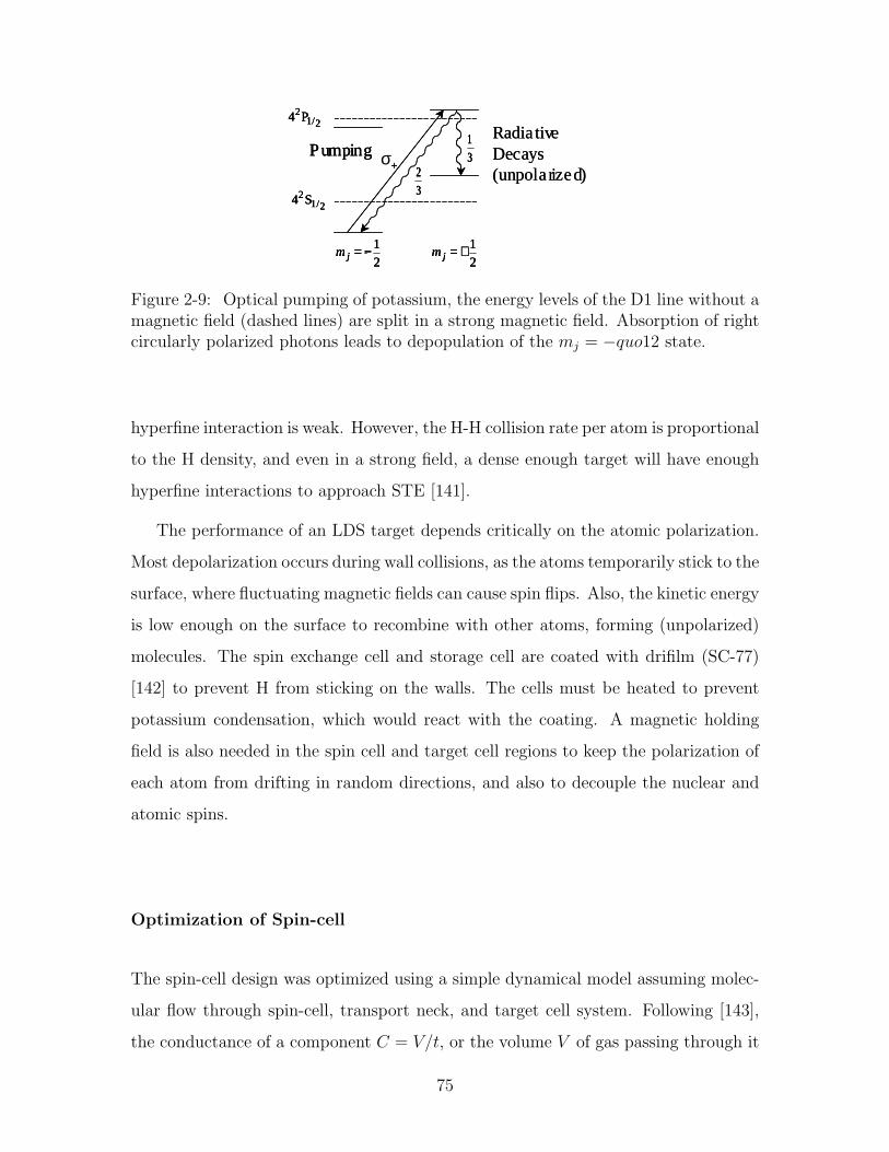
Radia tiveDecays(unpolarized)

σ+31

32

2

1+=jm2

1−=jm

2/12S4

2/12P4

PumpingRadia tiveDecays(unpolarized)

+31

32

2

1+=jm2

1−=jm

2/12S4

2/12P4

Pumping+

31

32

2

1+=jm2

1−=jm

2/12S4

2/12P4

Pumping

-

Figure 2-9: Optical pumping of potassium, the energy levels of the D1 line without amagnetic field (dashed lines) are split in a strong magnetic field. Absorption of rightcircularly polarized photons leads to depopulation of the mj = −quo12 state.

hyperfine interaction is weak. However, the H-H collision rate per atom is proportional

to the H density, and even in a strong field, a dense enough target will have enough

hyperfine interactions to approach STE [141].

The performance of an LDS target depends critically on the atomic polarization.

Most depolarization occurs during wall collisions, as the atoms temporarily stick to the

surface, where fluctuating magnetic fields can cause spin flips. Also, the kinetic energy

is low enough on the surface to recombine with other atoms, forming (unpolarized)

molecules. The spin exchange cell and storage cell are coated with drifilm (SC-77)

[142] to prevent H from sticking on the walls. The cells must be heated to prevent

potassium condensation, which would react with the coating. A magnetic holding

field is also needed in the spin cell and target cell regions to keep the polarization of

each atom from drifting in random directions, and also to decouple the nuclear and

atomic spins.

Optimization of Spin-cell

The spin-cell design was optimized using a simple dynamical model assuming molec-

ular flow through spin-cell, transport neck, and target cell system. Following [143],

the conductance of a component C = V/t, or the volume V of gas passing through it

75

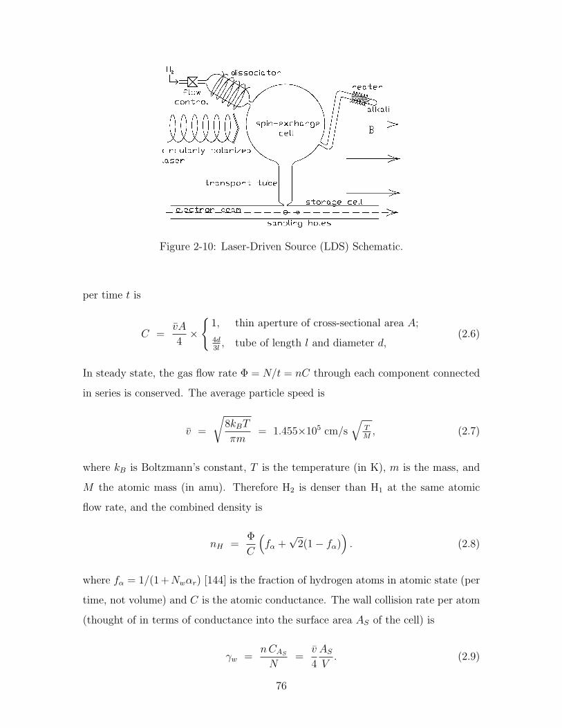
Figure 2-10: Laser-Driven Source (LDS) Schematic.

per time t is

C =vA

4×

1, thin aperture of cross-sectional area A;

4d3l

, tube of length l and diameter d,(2.6)

In steady state, the gas flow rate Φ = N/t = nC through each component connected

in series is conserved. The average particle speed is

v =

√8kBT

πm= 1.455×105 cm/s

√TM

, (2.7)

where kB is Boltzmann’s constant, T is the temperature (in K), m is the mass, and

M the atomic mass (in amu). Therefore H2 is denser than H1 at the same atomic

flow rate, and the combined density is

nH =Φ

C

(fα +

√2(1− fα)

). (2.8)

where fα = 1/(1+Nwαr) [144] is the fraction of hydrogen atoms in atomic state (per

time, not volume) and C is the atomic conductance. The wall collision rate per atom

(thought of in terms of conductance into the surface area AS of the cell) is

γw =n CAS

N=

v

4

AS

V. (2.9)

76

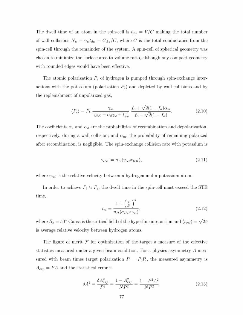
The dwell time of an atom in the spin-cell is tdw = V/C making the total number

of wall collisions Nw = γwtdw = CAS/C, where C is the total conductance from the

spin-cell through the remainder of the system. A spin-cell of spherical geometry was

chosen to minimize the surface area to volume ratio, although any compact geometry

with rounded edges would have been effective.

The atomic polarization Pe of hydrogen is pumped through spin-exchange inter-

actions with the potassium (polarization Pk) and depleted by wall collisions and by

the replenishment of unpolarized gas,

〈Pe〉 = Pkγse

γHK + αdγw + t−1dw

fα +√

2(1− fα)αm

fα +√

2(1− fα). (2.10)

The coefficients αr and αd are the probabilities of recombination and depolarization,

respectively, during a wall collision; and αm, the probability of remaining polarized

after recombination, is negligible. The spin-exchange collision rate with potassium is

γHK = nK〈vrelσHK〉, (2.11)

where vrel is the relative velocity between a hydrogen and a potassium atom.

In order to achieve Pt ≈ Pe, the dwell time in the spin-cell must exceed the STE

time,

tst =1 +

(BBc

)2

nH〈σHHvrel〉, (2.12)

where Bc = 507 Gauss is the critical field of the hyperfine interaction and 〈vrel〉 =√

2v

is average relative velocity between hydrogen atoms.

The figure of merit F for optimization of the target a measure of the effective

statistics measured under a given beam condition. For a physics asymmetry A mea-

sured with beam times target polarization P = PbPt, the measured asymmetry is

Aexp = PA and the statistical error is

δA2 =δA2

exp

P 2=

1− A2exp

NP 2=

1− P 2A2

NP 2. (2.13)

77

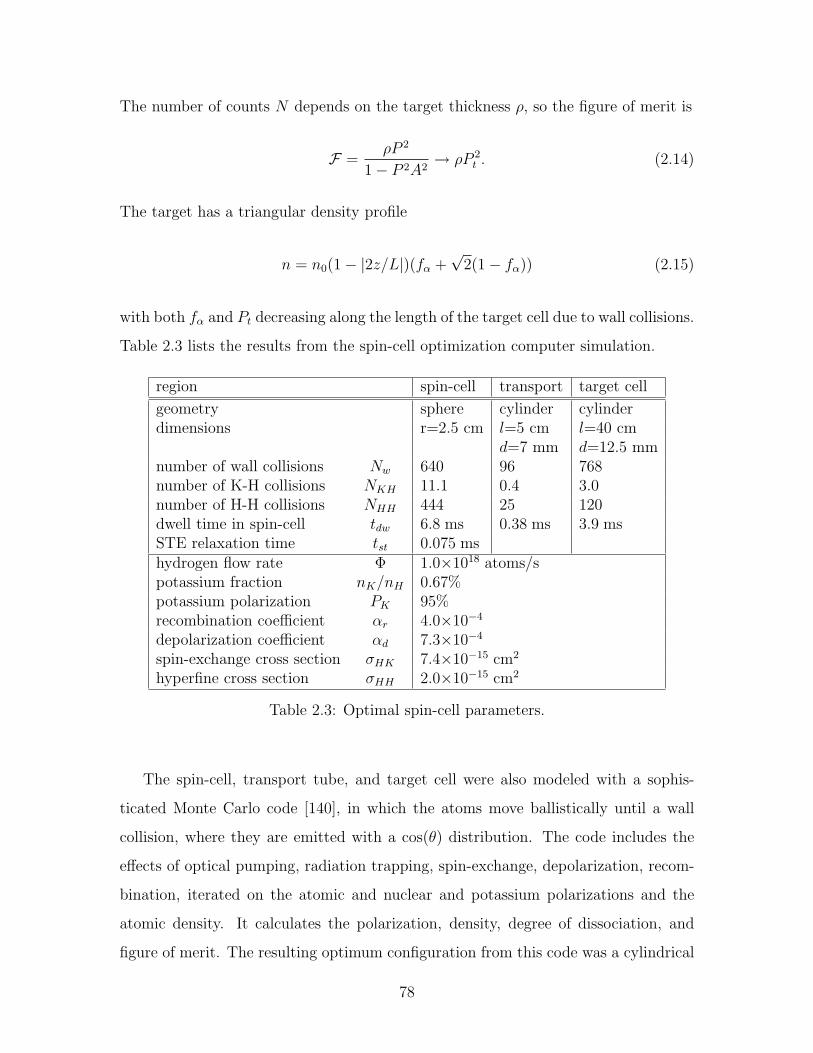
The number of counts N depends on the target thickness ρ, so the figure of merit is

F =ρP 2

1− P 2A2→ ρP 2

t . (2.14)

The target has a triangular density profile

n = n0(1− |2z/L|)(fα +√

2(1− fα)) (2.15)

with both fα and Pt decreasing along the length of the target cell due to wall collisions.

Table 2.3 lists the results from the spin-cell optimization computer simulation.

region spin-cell transport target cell

geometry sphere cylinder cylinderdimensions r=2.5 cm l=5 cm l=40 cm

d=7 mm d=12.5 mmnumber of wall collisions Nw 640 96 768number of K-H collisions NKH 11.1 0.4 3.0number of H-H collisions NHH 444 25 120dwell time in spin-cell tdw 6.8 ms 0.38 ms 3.9 msSTE relaxation time tst 0.075 mshydrogen flow rate Φ 1.0×1018 atoms/spotassium fraction nK/nH 0.67%potassium polarization PK 95%recombination coefficient αr 4.0×10−4

depolarization coefficient αd 7.3×10−4

spin-exchange cross section σHK 7.4×10−15 cm2

hyperfine cross section σHH 2.0×10−15 cm2

Table 2.3: Optimal spin-cell parameters.

The spin-cell, transport tube, and target cell were also modeled with a sophis-

ticated Monte Carlo code [140], in which the atoms move ballistically until a wall

collision, where they are emitted with a cos(θ) distribution. The code includes the

effects of optical pumping, radiation trapping, spin-exchange, depolarization, recom-

bination, iterated on the atomic and nuclear and potassium polarizations and the

atomic density. It calculates the polarization, density, degree of dissociation, and

figure of merit. The resulting optimum configuration from this code was a cylindrical

78

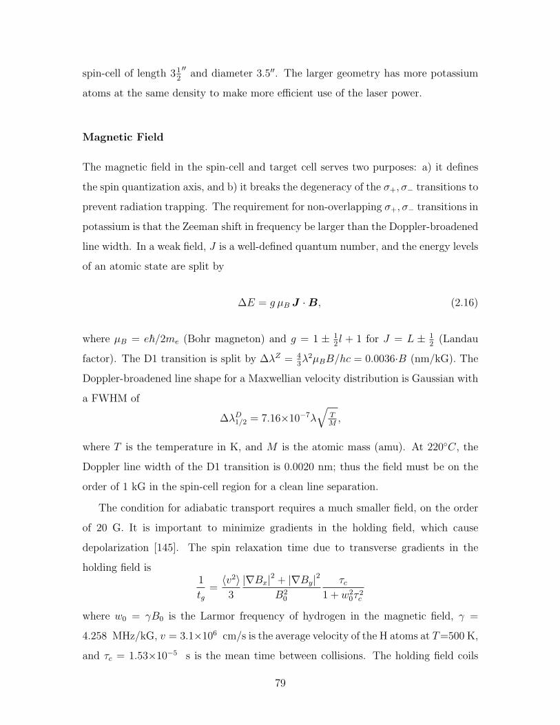
spin-cell of length 312

′′and diameter 3.5′′. The larger geometry has more potassium

atoms at the same density to make more efficient use of the laser power.

Magnetic Field

The magnetic field in the spin-cell and target cell serves two purposes: a) it defines

the spin quantization axis, and b) it breaks the degeneracy of the σ+, σ− transitions to

prevent radiation trapping. The requirement for non-overlapping σ+, σ− transitions in

potassium is that the Zeeman shift in frequency be larger than the Doppler-broadened

line width. In a weak field, J is a well-defined quantum number, and the energy levels

of an atomic state are split by

∆E = g µB J ·B, (2.16)

where µB = e~/2me (Bohr magneton) and g = 1 ± 12l + 1 for J = L ± 1

2(Landau

factor). The D1 transition is split by ∆λZ = 43λ2µBB/hc = 0.0036·B (nm/kG). The

Doppler-broadened line shape for a Maxwellian velocity distribution is Gaussian with

a FWHM of

∆λD1/2 = 7.16×10−7λ

√TM

,

where T is the temperature in K, and M is the atomic mass (amu). At 220C, the

Doppler line width of the D1 transition is 0.0020 nm; thus the field must be on the

order of 1 kG in the spin-cell region for a clean line separation.

The condition for adiabatic transport requires a much smaller field, on the order

of 20 G. It is important to minimize gradients in the holding field, which cause

depolarization [145]. The spin relaxation time due to transverse gradients in the

holding field is1

tg=〈v2〉3

|∇Bx|2 + |∇By|2

B20

τc

1 + w20τ

2c

where w0 = γB0 is the Larmor frequency of hydrogen in the magnetic field, γ =

4.258 MHz/kG, v = 3.1×106 cm/s is the average velocity of the H atoms at T=500 K,

and τc = 1.53×10−5 s is the mean time between collisions. The holding field coils

79

were designed to have gradients less than 13 G/cm, in which case the spin relaxation

time is tg = 0.26 s. This is much longer than the dwell time in the target, 3.9 ms.

Hardware Setup

The components of the LDS are shown in Fig. 2-11.

Figure 2-11: LDS Components: a) dissociator, b) potassium ampule, c) spin-cell(oven not shown), d) target cell, e) blank gasket apertures, f) permanent sextupolemagnet, g) chopper, h) quadrupole mass analyzer, i) 0.1T holding field coils, j) laserbeam for Faraday monitor, k) 3W Ti:Sapphire laser beam for optical pumping, l)beam expanding optics. The laser and magnetic field are are shown in the plane ofthe page for illustration purposes, but are actually rotated by 90 so as to extend outof the page.

The Pyrex spin-cell has two inlets, one for hydrogen, and the second for potassium.

It is connected to the target cell via a transport tube (neck). The end of the transport

tube is shaped to fit tightly against the storage cell. The spin-cell and target cells are

coated with a organosilane (SC-77 Drifilm) to prevent recombination and depolariza-

tion on the cell walls. The entire spin-cell and target cell must be uniformly heated

80

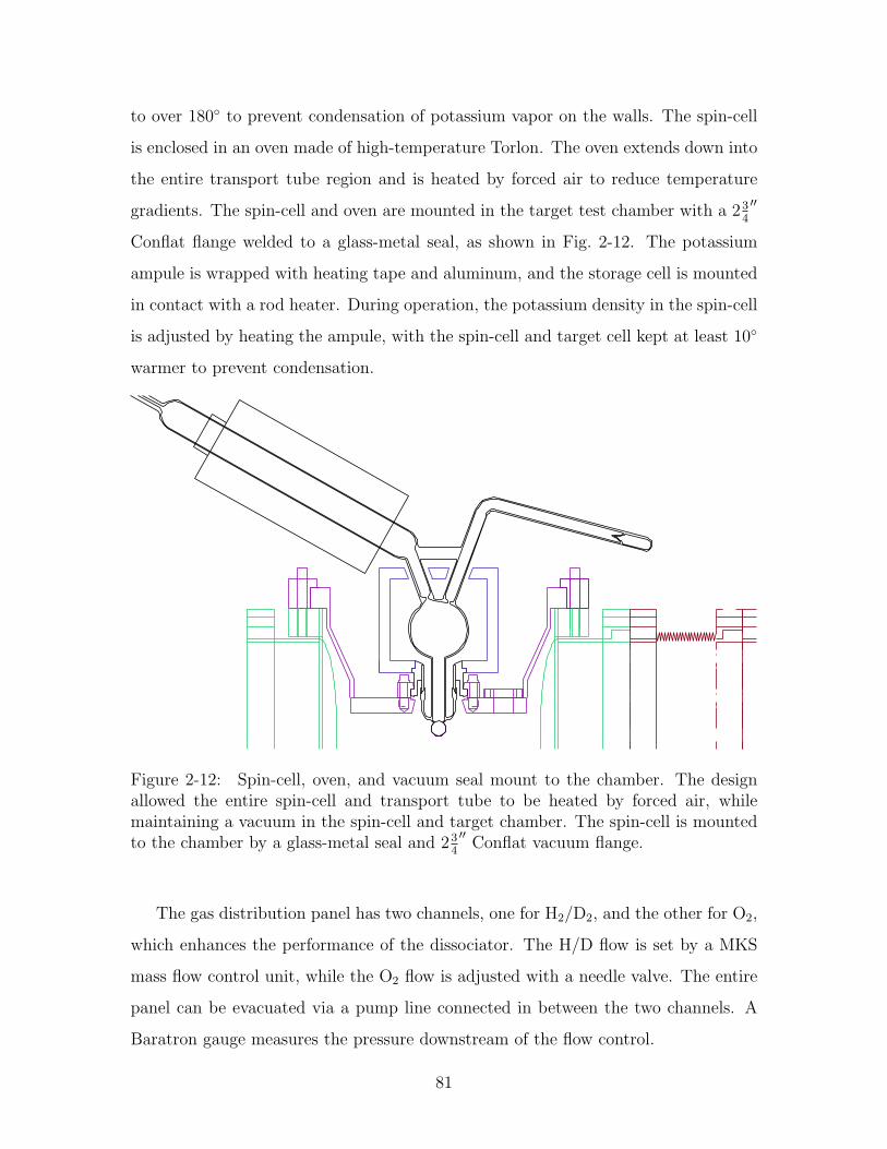
to over 180 to prevent condensation of potassium vapor on the walls. The spin-cell

is enclosed in an oven made of high-temperature Torlon. The oven extends down into

the entire transport tube region and is heated by forced air to reduce temperature

gradients. The spin-cell and oven are mounted in the target test chamber with a 234

′′

Conflat flange welded to a glass-metal seal, as shown in Fig. 2-12. The potassium

ampule is wrapped with heating tape and aluminum, and the storage cell is mounted

in contact with a rod heater. During operation, the potassium density in the spin-cell

is adjusted by heating the ampule, with the spin-cell and target cell kept at least 10

warmer to prevent condensation.

Figure 2-12: Spin-cell, oven, and vacuum seal mount to the chamber. The designallowed the entire spin-cell and transport tube to be heated by forced air, whilemaintaining a vacuum in the spin-cell and target chamber. The spin-cell is mountedto the chamber by a glass-metal seal and 23

4

′′Conflat vacuum flange.

The gas distribution panel has two channels, one for H2/D2, and the other for O2,

which enhances the performance of the dissociator. The H/D flow is set by a MKS

mass flow control unit, while the O2 flow is adjusted with a needle valve. The entire

panel can be evacuated via a pump line connected in between the two channels. A

Baratron gauge measures the pressure downstream of the flow control.

81

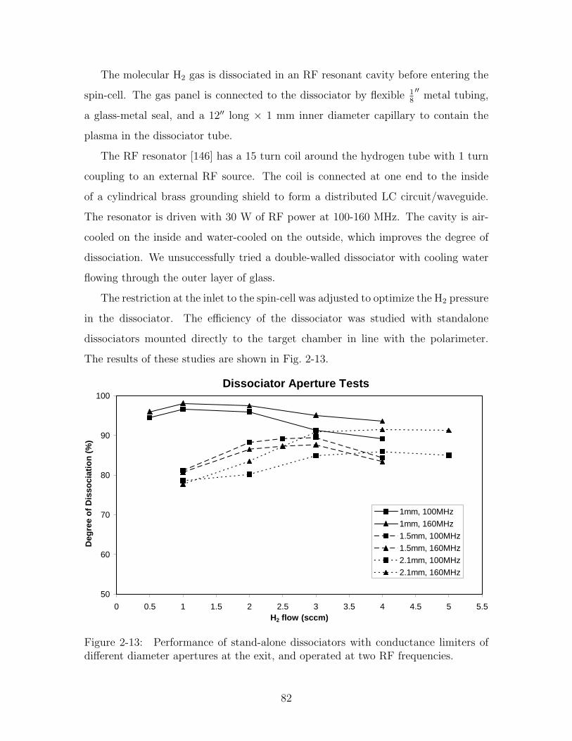
The molecular H2 gas is dissociated in an RF resonant cavity before entering the

spin-cell. The gas panel is connected to the dissociator by flexible 18

′′metal tubing,

a glass-metal seal, and a 12′′ long × 1 mm inner diameter capillary to contain the

plasma in the dissociator tube.

The RF resonator [146] has a 15 turn coil around the hydrogen tube with 1 turn

coupling to an external RF source. The coil is connected at one end to the inside

of a cylindrical brass grounding shield to form a distributed LC circuit/waveguide.

The resonator is driven with 30 W of RF power at 100-160 MHz. The cavity is air-

cooled on the inside and water-cooled on the outside, which improves the degree of

dissociation. We unsuccessfully tried a double-walled dissociator with cooling water

flowing through the outer layer of glass.

The restriction at the inlet to the spin-cell was adjusted to optimize the H2 pressure

in the dissociator. The efficiency of the dissociator was studied with standalone

dissociators mounted directly to the target chamber in line with the polarimeter.

The results of these studies are shown in Fig. 2-13.

Dissociator Aperture Tests

50

60

70

80

90

100

0 0.5 1 1.5 2 2.5 3 3.5 4 4.5 5 5.5H2 flow (sccm)

Deg

ree

of

Dis

soci

atio

n (

%)

1mm, 100MHz

1mm, 160MHz

1.5mm, 100MHz

1.5mm, 160MHz

2.1mm, 100MHz

2.1mm, 160MHz

Figure 2-13: Performance of stand-alone dissociators with conductance limiters ofdifferent diameter apertures at the exit, and operated at two RF frequencies.

82

The target chamber was designed for flexibility to accommodate various configu-

rations. The vacuum chamber a six way cross with 10′′ Conflat (CF) flanges on the

top and bottom, and 8′′ CF flanges on each side. The rear port is connected to a

Varian 1000HT turbo pump separated from the chamber and magnetic field by a 1 m

extension pipe. The port on the right side couples to the polarimeter, and the other

two side ports are used for feed-throughs and access to the chamber. The chamber is

equipped with Granville-Phillips thermocouple and Stabil-Ion pressure gauges, and

power and thermocouple feed-throughs for control of the target cell temperature. The

spin-cell is mounted to an inverted cone on the top, recessing down into the chamber.

The turbo pump and polarimeter are isolated by MDC 8′′ gate valves. The entire sys-

tem of gas valves, vacuum gauges and valves, pumps, shutters, and Quadrupole Mass

Analyzer (QMA) are automated by a custom electronic interface to LabVIEW with

hardwired interlock circuits to protect the components in the case of power failure or

software errors.

The LDS has two Helmholtz-like coils 12′′ apart with an 18′′ inner diameter. Each

of the two coils is composed of 144 turns of 38

′′hollow water-cooled copper conductor.

The coils draw 286 A at 50 V for a 1 kG field in the center of the spin-cell.

The laser system comprises a Spectra Physics 3900 Ti:Sapphire laser pumped

with a 20 W Argon laser. The Ti:Sapphire laser has three elements for tuning the

wavelength: a birefringent filter for coarse tuning, a thin etalon, and a thick etalon

for fine tuning. The thick etalon is heated in an oven to control the wavelength up

to 0.001 nm, and has line spacing of 0.040 nm. The oven temperature controller

electronics were modified to accept an analog control signal from the computer. Thus

the wavelength can be scanned through the σ+ and σ− D1 resonance lines. The thin

etalon has a line thickness of 0.040 nm and has a manual threaded adjustment to

select the range of the thick etalon. Similarly the birefringent filter angle is adjusted

by hand to select the range of thin etalon line. A small fraction of the beam is split

into a power meter and a wave-meter which is accurate to 0.001 nm. The line width

is also monitored with a spectrum analyzer. All three diagnostics are recorded in

LabVIEW.

83

The laser beam is passed through a Conoptics M360-50 Electrical-Optic Modulator

(EOM) to broaden the narrow line-width to match the Doppler-broadened profile of

the potassium absorption line. The EOM contains two crystals of Lithium Tantalate

(LiTaO3) with a diameter of 1.25 mm and combined length of 40 mm. It can handle

up to 2.5 W of beam which must be focused fine enough to pass through the crystal,

but diffuse enough not to burn the crystal. The modulator is driven by 20-450 MHz

white noise from an Accu-Noise generator amplified to 20 W by a Minicircuits LZY-

1 amplifier. The resulting line-width is about 1 GHz FWHM, which enhances the

absorption of laser power by about 30%.

The beam is expanded to a diameter of 5 cm to fill the cross sectional area of the

spin-cell. It passes through a linear polarizer and a λ/4 wave-plate to achieve circular

polarization. The beam is periscoped down into the sunken spin-cell with two 45

polarization preserving mirrors, as there is no room for a polarization compensating

optical setup. The transmitted beam through the spin-cell is monitored on the other

end with a power monitor.

Both the dissociation fraction fα and atomic polarization Pe are measured with

a Stern-Gerlach type polarimeter. The polarimeter has two chambers separated by

blank Conflat gaskets with a 3 mm hole in the center of each to collimate the atoms

which escape from the sampling holes in the target cell. The apertures also serve

as conductance limiters, and the polarimeter is differentially pumped with a Varian

300 L/s ion pump in each chamber and a NEG pump in the final chamber. The

polarimeter is coupled to the target chamber by a 6′′ metal bellows section for two

way alignment. The polarimeter is supported by a gimbal connected around the

bellows to the target chamber, and balances on two load-bearing frictionless pads.

The first chamber has a shutter and a sextupole for filtering spin-states. The

sextupole is 10 cm long with an outer diameter of 25 mm and a 5 mm tapered bore.

The field strength at the pole tips is about 1.5 T. Simulations were done to determine

the optimum distance of the sextupole from the detector.

The second chamber contains a chopper and Quadrupole Mass Analyzer (QMA)

for measurement of the beam intensity. The chopper is a 3/8′′ steel rod with a slot

84

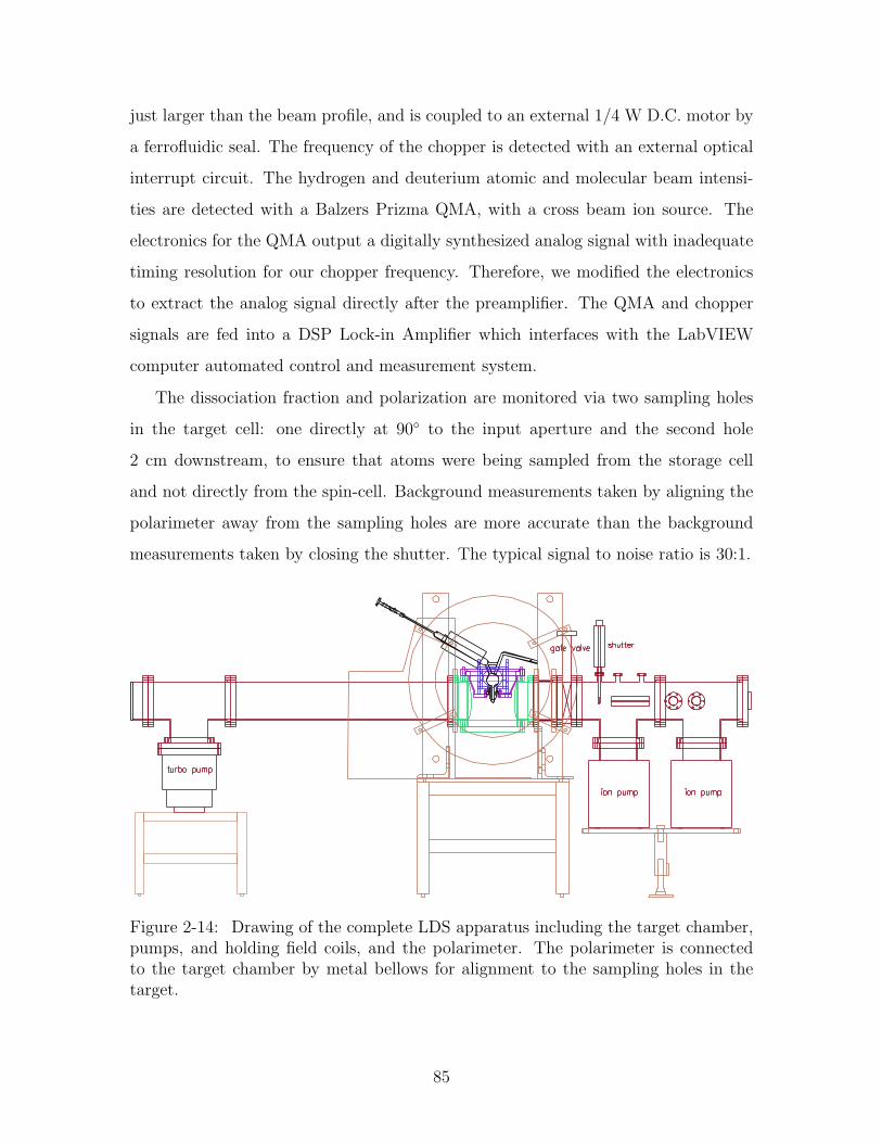
just larger than the beam profile, and is coupled to an external 1/4 W D.C. motor by

a ferrofluidic seal. The frequency of the chopper is detected with an external optical

interrupt circuit. The hydrogen and deuterium atomic and molecular beam intensi-

ties are detected with a Balzers Prizma QMA, with a cross beam ion source. The

electronics for the QMA output a digitally synthesized analog signal with inadequate

timing resolution for our chopper frequency. Therefore, we modified the electronics

to extract the analog signal directly after the preamplifier. The QMA and chopper

signals are fed into a DSP Lock-in Amplifier which interfaces with the LabVIEW

computer automated control and measurement system.

The dissociation fraction and polarization are monitored via two sampling holes

in the target cell: one directly at 90 to the input aperture and the second hole

2 cm downstream, to ensure that atoms were being sampled from the storage cell

and not directly from the spin-cell. Background measurements taken by aligning the

polarimeter away from the sampling holes are more accurate than the background

measurements taken by closing the shutter. The typical signal to noise ratio is 30:1.

Figure 2-14: Drawing of the complete LDS apparatus including the target chamber,pumps, and holding field coils, and the polarimeter. The polarimeter is connectedto the target chamber by metal bellows for alignment to the sampling holes in thetarget.

85

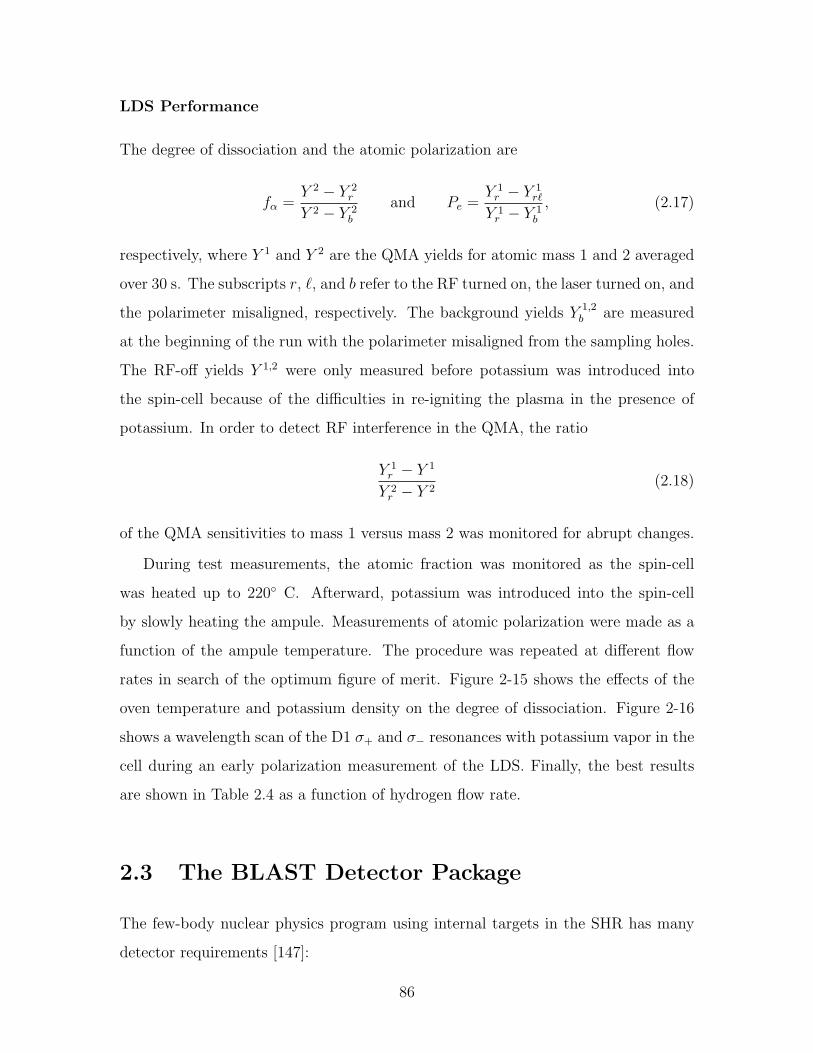
LDS Performance

The degree of dissociation and the atomic polarization are

fα =Y 2 − Y 2

r

Y 2 − Y 2b

and Pe =Y 1

r − Y 1r`

Y 1r − Y 1

b

, (2.17)

respectively, where Y 1 and Y 2 are the QMA yields for atomic mass 1 and 2 averaged

over 30 s. The subscripts r, `, and b refer to the RF turned on, the laser turned on, and

the polarimeter misaligned, respectively. The background yields Y 1,2b are measured

at the beginning of the run with the polarimeter misaligned from the sampling holes.

The RF-off yields Y 1,2 were only measured before potassium was introduced into

the spin-cell because of the difficulties in re-igniting the plasma in the presence of

potassium. In order to detect RF interference in the QMA, the ratio

Y 1r − Y 1

Y 2r − Y 2

(2.18)

of the QMA sensitivities to mass 1 versus mass 2 was monitored for abrupt changes.

During test measurements, the atomic fraction was monitored as the spin-cell

was heated up to 220 C. Afterward, potassium was introduced into the spin-cell

by slowly heating the ampule. Measurements of atomic polarization were made as a

function of the ampule temperature. The procedure was repeated at different flow

rates in search of the optimum figure of merit. Figure 2-15 shows the effects of the

oven temperature and potassium density on the degree of dissociation. Figure 2-16

shows a wavelength scan of the D1 σ+ and σ− resonances with potassium vapor in the

cell during an early polarization measurement of the LDS. Finally, the best results

are shown in Table 2.4 as a function of hydrogen flow rate.

2.3 The BLAST Detector Package

The few-body nuclear physics program using internal targets in the SHR has many

detector requirements [147]:

86

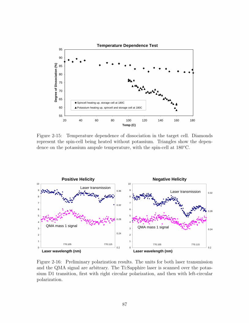
Temperature Dependence Test

55

60

65

70

75

80

85

90

95

20 40 60 80 100 120 140 160 180

Temp (C)

Deg

ree

of

Dis

soci

atio

n (

%)

Spincell heating up, storage cell at 180C

Potassium heating up, spincell and storage cell at 180C

Figure 2-15: Temperature dependence of dissociation in the target cell. Diamondsrepresent the spin-cell being heated without potassium. Triangles show the depen-dence on the potassium ampule temperature, with the spin-cell at 180C.

Positive Helicity

0

1

2

3

4

5

6

7

8

9

10

Laser wavelength (nm)0.2

0.24

0.28

0.32

0.36Laser transmission

QMA mass 1 signal

770.105 770.115

Negative Helicity

0

1

2

3

4

5

6

7

8

9

10

Laser wavelength (nm)0.2

0.24

0.28

0.32Laser transmission

QMA mass 1 signal

770.105 770.115

Figure 2-16: Preliminary polarization results. The units for both laser transmissionand the QMA signal are arbitrary. The Ti:Sapphire laser is scanned over the potas-sium D1 transition, first with right circular polarization, and then with left-circularpolarization.

87

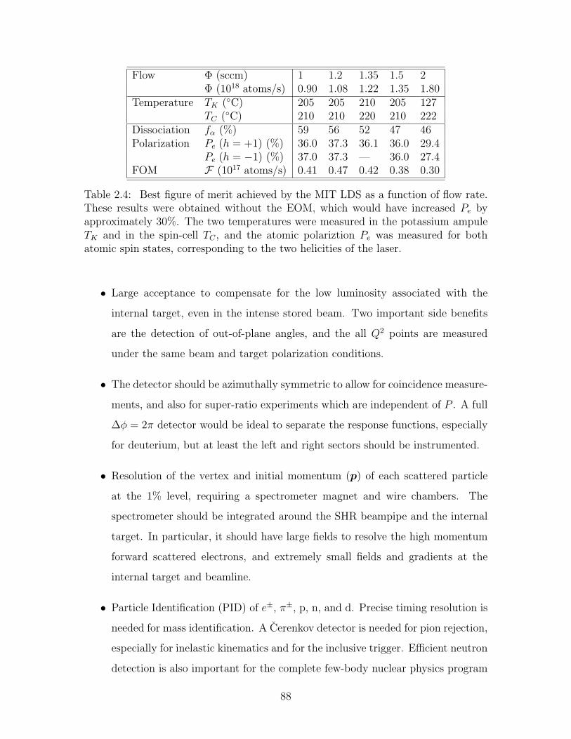
Flow Φ (sccm) 1 1.2 1.35 1.5 2Φ (1018 atoms/s) 0.90 1.08 1.22 1.35 1.80

Temperature TK (C) 205 205 210 205 127TC (C) 210 210 220 210 222

Dissociation fα (%) 59 56 52 47 46Polarization Pe (h = +1) (%) 36.0 37.3 36.1 36.0 29.4

Pe (h = −1) (%) 37.0 37.3 — 36.0 27.4FOM F (1017 atoms/s) 0.41 0.47 0.42 0.38 0.30

Table 2.4: Best figure of merit achieved by the MIT LDS as a function of flow rate.These results were obtained without the EOM, which would have increased Pe byapproximately 30%. The two temperatures were measured in the potassium ampuleTK and in the spin-cell TC , and the atomic polariztion Pe was measured for bothatomic spin states, corresponding to the two helicities of the laser.

• Large acceptance to compensate for the low luminosity associated with the

internal target, even in the intense stored beam. Two important side benefits

are the detection of out-of-plane angles, and the all Q2 points are measured

under the same beam and target polarization conditions.

• The detector should be azimuthally symmetric to allow for coincidence measure-

ments, and also for super-ratio experiments which are independent of P . A full

∆φ = 2π detector would be ideal to separate the response functions, especially

for deuterium, but at least the left and right sectors should be instrumented.

• Resolution of the vertex and initial momentum (p) of each scattered particle

at the 1% level, requiring a spectrometer magnet and wire chambers. The

spectrometer should be integrated around the SHR beampipe and the internal

target. In particular, it should have large fields to resolve the high momentum

forward scattered electrons, and extremely small fields and gradients at the

internal target and beamline.

• Particle Identification (PID) of e±, π±, p, n, and d. Precise timing resolution is

needed for mass identification. A Cerenkov detector is needed for pion rejection,

especially for inelastic kinematics and for the inclusive trigger. Efficient neutron

detection is also important for the complete few-body nuclear physics program

88

including neutron form factors.

In conformance with these requirements, the detector package was designed around

eight coils of the Bates Large Acceptance Spectrometer Toroid (BLAST) magnet.

The two horizontal sectors are instrumented with, from the beam line radially out-

ward: drift chambers, Cerenkov detectors, time-of-flight (TOF) scintillators, and two

sets of neutron scintillators. The top and bottom sectors contain the ABS and di-

agnostics. To minimize costs the other four sectors are left open. Both the BLAST

coils and detector sub-packages are installed on rails to open for maintenance. The

spectrometer toroid and each of these detectors are shown in Fig. 2-17. Each detector

except the neutron scintillators [133] is explained in further detail in this section.

The BLAST detector was built using conventional technology for cost reduction

and reliability. The scintillators, Cerenkov detectors, and wire chambers were all

based on standard designs. The trigger was based on the trigger for Hall A at JLab.

The data acquisition software CODA was written at JLab and most of the trigger

and readout electronics were based on the VME and FASTBUS hardware also used

at JLab. All computing power was based on inexpensive PCs running Linux, includ-

ing the 40 CPU analysis cluster. The slow control system is based on the industry

standard EPICS used elsewhere throughout the lab. Finally, the simulation, recon-

struction, and analysis software is based on the CERN packages GEANT and ROOT.

The BLAST coordinate system is defined with the origin at the center of the in-

ternal target, the z-axis pointing downstream along the beamline, the y-axis pointing

straight up, and the x-axis in the horizontal plane outward in the left sector (looking

downstream). Spherical and cylindrical coordinates in the BLAST frame are defined

as usual:

x = ρ sin φ, y = ρ cos φ, z = r cos θ, and ρ = r sin θ. (2.19)

Each detector element also has its own coordinate system with the origin in the center

of the detector, the x′-axis running horizontally along the face of the detector in the

direction of increasing θ, the y′-axis pointing either up or down in the direction of

89

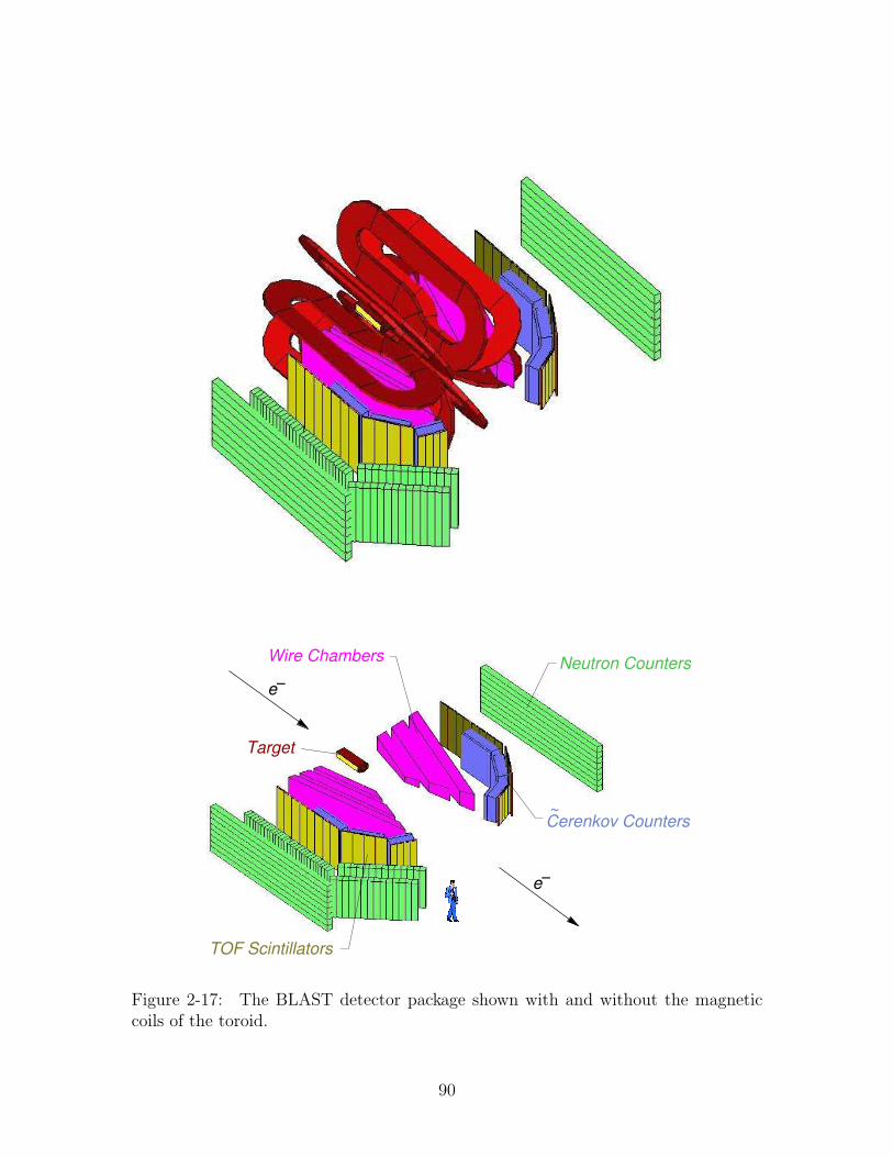
e−

e−

Wire Chambers

Cerenkov Counters~

Target

TOF Scintillators

Neutron Counters

Figure 2-17: The BLAST detector package shown with and without the magneticcoils of the toroid.

90

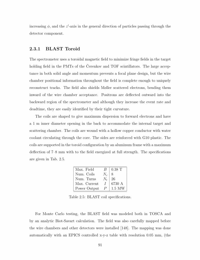
increasing φ, and the z′-axis in the general direction of particles passing through the

detector component.

2.3.1 BLAST Toroid

The spectrometer uses a toroidal magnetic field to minimize fringe fields in the target

holding field in the PMTs of the Cerenkov and TOF scintillators. The large accep-

tance in both solid angle and momentum prevents a focal plane design, but the wire

chamber positional information throughout the field is complete enough to uniquely

reconstruct tracks. The field also shields Møller scattered electrons, bending them

inward of the wire chamber acceptance. Positrons are deflected outward into the

backward region of the spectrometer and although they increase the event rate and

deadtime, they are easily identified by their tight curvature.

The coils are shaped to give maximum dispersion to forward electrons and have

a 1 m inner diameter opening in the back to accommodate the internal target and

scattering chamber. The coils are wound with a hollow copper conductor with water

coolant circulating through the core. The sides are reinforced with G10 plastic. The

coils are supported in the toroid configuration by an aluminum frame with a maximum

deflection of 7–8 mm with to the field energized at full strength. The specifications

are given in Tab. 2.5.

Max. Field B 0.38 TNum. Coils Nc 8Num. Turns Nt 26Max. Current I 6730 APower Output P 1.5 MW

Table 2.5: BLAST coil specifications.

For Monte Carlo testing, the BLAST field was modeled both in TOSCA and

by an analytic Biot-Savart calculation. The field was also carefully mapped before

the wire chambers and other detectors were installed [148]. The mapping was done

automatically with an EPICS controlled x-y-z table with resolution 0.05 mm, (the

91

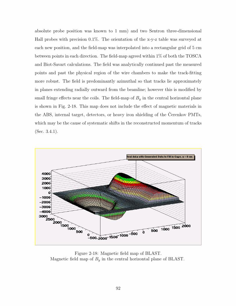
absolute probe position was known to 1 mm) and two Sentron three-dimensional

Hall probes with precision 0.1%. The orientation of the x-y-z table was surveyed at

each new position, and the field-map was interpolated into a rectangular grid of 5 cm

between points in each direction. The field-map agreed within 1% of both the TOSCA

and Biot-Savart calculations. The field was analytically continued past the measured

points and past the physical region of the wire chambers to make the track-fitting

more robust. The field is predominantly azimuthal so that tracks lie approximately

in planes extending radially outward from the beamline; however this is modified by

small fringe effects near the coils. The field-map of By in the central horizontal plane

is shown in Fig. 2-18. This map does not include the effect of magnetic materials in

the ABS, internal target, detectors, or heavy iron shielding of the Cerenkov PMTs,

which may be the cause of systematic shifts in the reconstructed momentum of tracks

(Sec. 3.4.1).

Figure 2-18: Magnetic field map of BLAST.Magnetic field map of By in the central horizontal plane of BLAST.

92

2.3.2 Drift Chambers

The drift chambers (WC) are embedded in the φ = ±22.5 horizontal sectors between

the toroid coils and were designed to maximize the acceptance within these con-

straints. The three chambers in each sector were constructed of one-piece aluminum

frames joined together with spacers to form a single airtight chamber. A mixture of

helium and isobutane flows through the chambers at just above atmospheric pressure.

This single-chamber aluminum construction was chosen over lower-cost G10 layered

frames because of its strength against deformation from the wire tension. Multiple

scattering is reduced by the elimination of windows between each chamber, by the

use of field and guard wires instead of foil cathodes, and the use of helium instead

of air as the quenching gas. The chambers are planar at an angle of α = 16.5 with

respect to the beam-line, and the frame has a trapezoidal shape on all 6 faces.

In general, a particle track through the spectrometer has 5 degrees of freedom: its

momentum p = (p, θ, φ) and position x = (x, y, z) at a fixed point along the trajectory

modulo one free parameter along the length of the track. We use the interaction vertex

parameters (p, θ, φ, z, d) for physics analysis and the trajectory at the wire chamber

entrance plane (pw, θw, φw, xw, yw) for reconstruction purposes. The parameter z is

the location of the interaction vertex in BLAST coordinates, calculated as the closest

point to the track along the beamline. The distance d of closest approach to the

z-axis (beam line) is fixed at d = 0, since the beam position is known much better

than the wire chamber resolution. Likewise, there is a constraint between φw and

yw. Therefore the wire chambers must determine four independent track parameters.

Hits are required in each of the three chambers for momentum resolution. In practice,

at least 12 hits are required for adequate track reconstruction. In the wire chamber

(WC) coordinates, xw is along the face of the wire chamber in the horizontal plane

and increases with θ (toward upstream), yw points straight up or down and increases

with φ, and zw is perpendicular to the wire planes directed away from the beamline.

Each chamber contains two superlayers of cells rotated about the zw-axis by the

stereo angles +5 (inner) and −5 (outer) for two dimensional track coordinates in

93

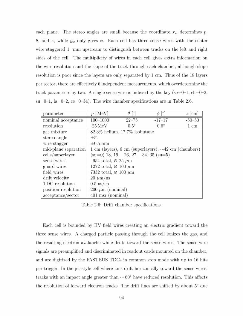
each plane. The stereo angles are small because the coordinate xw determines p,

θ, and z, while yw only gives φ. Each cell has three sense wires with the center

wire staggered 1 mm upstream to distinguish between tracks on the left and right

sides of the cell. The multiplicity of wires in each cell gives extra information on

the wire resolution and the slope of the track through each chamber, although slope

resolution is poor since the layers are only separated by 1 cm. Thus of the 18 layers

per sector, there are effectively 6 independent measurements, which overdetermine the

track parameters by two. A single sense wire is indexed by the key (se=0–1, ch=0–2,

su=0–1, la=0–2, ce=0–34). The wire chamber specifications are in Table 2.6.

parameter p [ MeV] θ [] φ [] z [cm]

nominal acceptance 100–1000 22–75 -17–17 -50–50resolution 25 MeV 0.5 0.6 1 cmgas mixture 82.3% helium, 17.7% isobutanestereo angle ±5

wire stagger ±0.5 mmmid-plane separation 1 cm (layers), 6 cm (superlayers), ∼42 cm (chambers)cells/superlayer (su=0) 18, 19, 26, 27, 34, 35 (su=5)sense wires 954 total, ∅ 25 µmguard wires 1272 total, ∅ 100 µmfield wires 7332 total, ∅ 100 µmdrift velocity 20 µm/nsTDC resolution 0.5 ns/chposition resolution 200 µm (nominal)acceptance/sector 401 msr (nominal)

Table 2.6: Drift chamber specifications.

Each cell is bounded by HV field wires creating an electric gradient toward the

three sense wires. A charged particle passing through the cell ionizes the gas, and

the resulting electron avalanche while drifts toward the sense wires. The sense wire

signals are preamplified and discriminated in readout cards mounted on the chamber,

and are digitized by the FASTBUS TDCs in common stop mode with up to 16 hits

per trigger. In the jet-style cell where ions drift horizontally toward the sense wires,

tracks with an impact angle greater than ∼ 60 have reduced resolution. This affects

the resolution of forward electron tracks. The drift lines are shifted by about 5 due

94

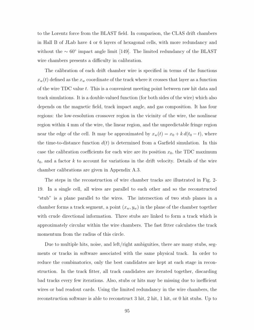
to the Lorentz force from the BLAST field. In comparison, the CLAS drift chambers

in Hall B of JLab have 4 or 6 layers of hexagonal cells, with more redundancy and

without the ∼ 60 impact angle limit [149]. The limited redundancy of the BLAST

wire chambers presents a difficulty in calibration.

The calibration of each drift chamber wire is specified in terms of the functions

xw(t) defined as the xw coordinate of the track where it crosses that layer as a function

of the wire TDC value t. This is a convenient meeting point between raw hit data and

track simulations. It is a double-valued function (for both sides of the wire) which also

depends on the magnetic field, track impact angle, and gas composition. It has four

regions: the low-resolution crossover region in the vicinity of the wire, the nonlinear

region within 4 mm of the wire, the linear region, and the unpredictable fringe region

near the edge of the cell. It may be approximated by xw(t) = x0 + k d(t0 − t), where

the time-to-distance function d(t) is determined from a Garfield simulation. In this

case the calibration coefficients for each wire are its position x0, the TDC maximum

t0, and a factor k to account for variations in the drift velocity. Details of the wire

chamber calibrations are given in Appendix A.3.

The steps in the reconstruction of wire chamber tracks are illustrated in Fig. 2-

19. In a single cell, all wires are parallel to each other and so the reconstructed

“stub” is a plane parallel to the wires. The intersection of two stub planes in a

chamber forms a track segment, a point (xw, yw) in the plane of the chamber together

with crude directional information. Three stubs are linked to form a track which is

approximately circular within the wire chambers. The fast fitter calculates the track

momentum from the radius of this circle.

Due to multiple hits, noise, and left/right ambiguities, there are many stubs, seg-

ments or tracks in software associated with the same physical track. In order to

reduce the combinatorics, only the best candidates are kept at each stage in recon-

struction. In the track fitter, all track candidates are iterated together, discarding

bad tracks every few iterations. Also, stubs or hits may be missing due to inefficient

wires or bad readout cards. Using the limited redundancy in the wire chambers, the

reconstruction software is able to reconstruct 3 hit, 2 hit, 1 hit, or 0 hit stubs. Up to

95

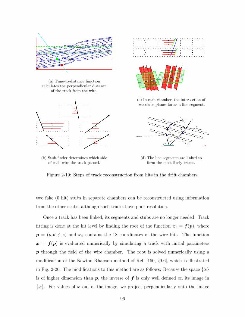
(a) Time-to-distance functioncalculates the perpendicular distance

of the track from the wire.

(b) Stub-finder determines which sideof each wire the track passed.

(c) In each chamber, the intersection oftwo stubs planes forms a line segment.

(d) The line segments are linked toform the most likely tracks.

Figure 2-19: Steps of track reconstruction from hits in the drift chambers.

two fake (0 hit) stubs in separate chambers can be reconstructed using information

from the other stubs, although such tracks have poor resolution.

Once a track has been linked, its segments and stubs are no longer needed. Track

fitting is done at the hit level by finding the root of the function x0 = f(p), where

p = (p, θ, φ, z) and x0 contains the 18 coordinates of the wire hits. The function

x = f(p) is evaluated numerically by simulating a track with initial parameters

p through the field of the wire chamber. The root is solved numerically using a

modification of the Newton-Rhapson method of Ref. [150, §9.6], which is illustrated

in Fig. 2-20. The modifications to this method are as follows: Because the space x

is of higher dimension than p, the inverse of f is only well defined on its image in

x. For values of x out of the image, we project perpendicularly onto the image

96

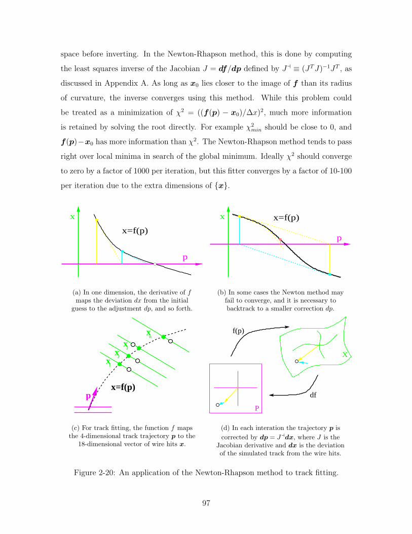
space before inverting. In the Newton-Rhapson method, this is done by computing

the least squares inverse of the Jacobian J = df/dp defined by Ja ≡ (JT J)−1JT , as

discussed in Appendix A. As long as x0 lies closer to the image of f than its radius

of curvature, the inverse converges using this method. While this problem could

be treated as a minimization of χ2 = ((f(p) − x0)/∆x)2, much more information

is retained by solving the root directly. For example χ2min should be close to 0, and

f(p)−x0 has more information than χ2. The Newton-Rhapson method tends to pass

right over local minima in search of the global minimum. Ideally χ2 should converge

to zero by a factor of 1000 per iteration, but this fitter converges by a factor of 10-100

per iteration due to the extra dimensions of x.

p

x

x=f(p)

(a) In one dimension, the derivative of fmaps the deviation dx from the initial

guess to the adjustment dp, and so forth.

x x=f(p)

p

(b) In some cases the Newton method mayfail to converge, and it is necessary tobacktrack to a smaller correction dp.

x2

x3

xn

p

x1

x=f(p)

(c) For track fitting, the function f mapsthe 4-dimensional track trajectory p to the

18-dimensional vector of wire hits x.

df

X

P

f(p)

(d) In each interation the trajectory p iscorrected by dp = Jadx, where J is the

Jacobian derivative and dx is the deviationof the simulated track from the wire hits.

Figure 2-20: An application of the Newton-Rhapson method to track fitting.

97

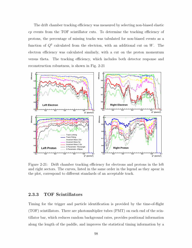
The drift chamber tracking efficiency was measured by selecting non-biased elastic

ep events from the TOF scintillator cuts. To determine the tracking efficiency of

protons, the percentage of missing tracks was tabulated for non-biased events as a

function of Q2 calculated from the electrion, with an additional cut on W . The

electron efficiency was calculated similarly, with a cut on the proton momentum

versus theta. The tracking efficiency, which includes both detector response and

reconstruction robustness, is shown in Fig. 2-21

]2 [(GeV/c)2Q0.1 0.2 0.3 0.4 0.5 0.6 0.7

Eff

icie

ncy

0.5

0.6

0.7

0.8

0.9

1

Left Electron

]2 [(GeV/c)2Q0.1 0.2 0.3 0.4 0.5 0.6 0.7

Eff

icie

ncy

0.5

0.6

0.7

0.8

0.9

1

Right Electron

]2 [(GeV/c)2Q0.1 0.2 0.3 0.4 0.5 0.6 0.7

Eff

icie

ncy

0.5

0.6

0.7

0.8

0.9

1

Left Proton

Track LinkingTrack Fitting

σInvariant Mass 10σInvariant Mass 5

σInvariant Mass 2.55 Parameter--Rectangle5 Parameter--Ellipse

]2 [(GeV/c)2Q0.1 0.2 0.3 0.4 0.5 0.6 0.7

Eff

icie

ncy

0.5

0.6

0.7

0.8

0.9

1

Right Proton

Figure 2-21: Drift chamber tracking efficiency for electrons and protons in the leftand right sectors. The curves, listed in the same order in the legend as they apear inthe plot, correspond to different standards of an acceptable track.

2.3.3 TOF Scintillators

Timing for the trigger and particle identification is provided by the time-of-flight

(TOF) scintillators. There are photomultiplier tubes (PMT) on each end of the scin-

tillator bar, which reduces random background rates, provides positional information

along the length of the paddle, and improves the statistical timing information by a

98

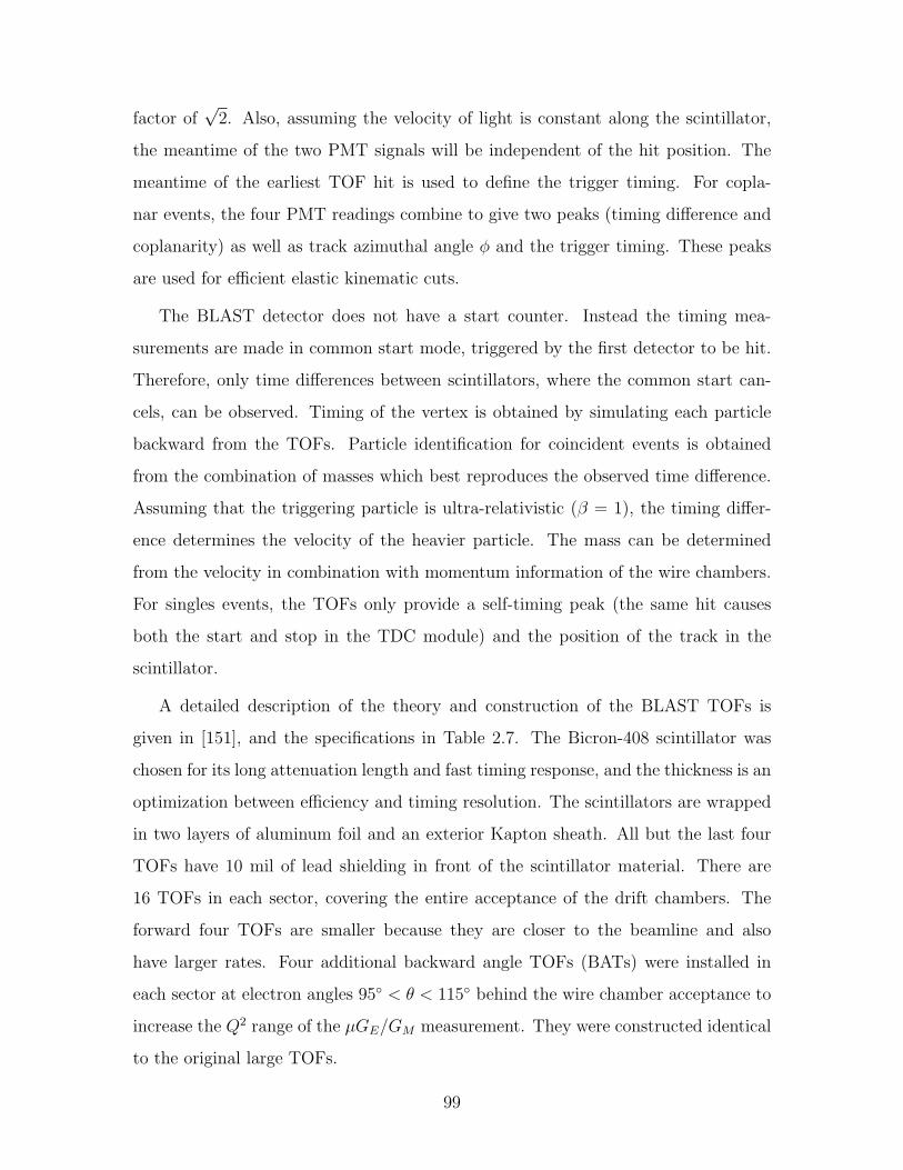
factor of√

2. Also, assuming the velocity of light is constant along the scintillator,

the meantime of the two PMT signals will be independent of the hit position. The

meantime of the earliest TOF hit is used to define the trigger timing. For copla-

nar events, the four PMT readings combine to give two peaks (timing difference and

coplanarity) as well as track azimuthal angle φ and the trigger timing. These peaks

are used for efficient elastic kinematic cuts.

The BLAST detector does not have a start counter. Instead the timing mea-

surements are made in common start mode, triggered by the first detector to be hit.

Therefore, only time differences between scintillators, where the common start can-

cels, can be observed. Timing of the vertex is obtained by simulating each particle

backward from the TOFs. Particle identification for coincident events is obtained

from the combination of masses which best reproduces the observed time difference.

Assuming that the triggering particle is ultra-relativistic (β = 1), the timing differ-

ence determines the velocity of the heavier particle. The mass can be determined

from the velocity in combination with momentum information of the wire chambers.

For singles events, the TOFs only provide a self-timing peak (the same hit causes

both the start and stop in the TDC module) and the position of the track in the

scintillator.

A detailed description of the theory and construction of the BLAST TOFs is

given in [151], and the specifications in Table 2.7. The Bicron-408 scintillator was

chosen for its long attenuation length and fast timing response, and the thickness is an

optimization between efficiency and timing resolution. The scintillators are wrapped

in two layers of aluminum foil and an exterior Kapton sheath. All but the last four

TOFs have 10 mil of lead shielding in front of the scintillator material. There are

16 TOFs in each sector, covering the entire acceptance of the drift chambers. The

forward four TOFs are smaller because they are closer to the beamline and also

have larger rates. Four additional backward angle TOFs (BATs) were installed in

each sector at electron angles 95 < θ < 115 behind the wire chamber acceptance to

increase the Q2 range of the µGE/GM measurement. They were constructed identical

to the original large TOFs.

99

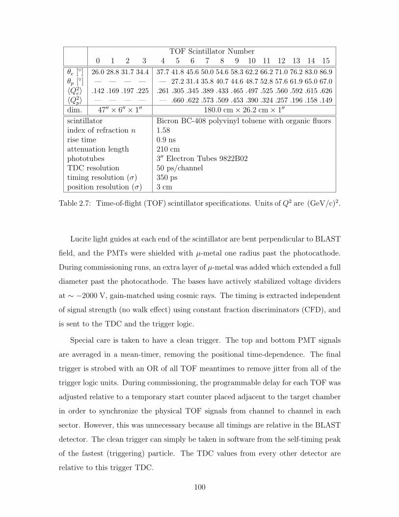
TOF Scintillator Number0 1 2 3 4 5 6 7 8 9 10 11 12 13 14 15

θe [] 26.0 28.8 31.7 34.4 37.7 41.8 45.6 50.0 54.6 58.3 62.2 66.2 71.0 76.2 83.0 86.9θp [] — — — — — 27.2 31.4 35.8 40.7 44.6 48.7 52.8 57.6 61.9 65.0 67.0〈Q2

e〉 .142 .169 .197 .225 .261 .305 .345 .389 .433 .465 .497 .525 .560 .592 .615 .626〈Q2

p〉 — — — — — .660 .622 .573 .509 .453 .390 .324 .257 .196 .158 .149dim. 47′′ × 6′′ × 1′′ 180.0 cm× 26.2 cm× 1′′

scintillator Bicron BC-408 polyvinyl toluene with organic fluorsindex of refraction n 1.58rise time 0.9 nsattenuation length 210 cmphototubes 3′′ Electron Tubes 9822B02TDC resolution 50 ps/channeltiming resolution (σ) 350 psposition resolution (σ) 3 cm

Table 2.7: Time-of-flight (TOF) scintillator specifications. Units of Q2 are (GeV/c)2.

Lucite light guides at each end of the scintillator are bent perpendicular to BLAST

field, and the PMTs were shielded with µ-metal one radius past the photocathode.

During commissioning runs, an extra layer of µ-metal was added which extended a full

diameter past the photocathode. The bases have actively stabilized voltage dividers

at ∼ −2000 V, gain-matched using cosmic rays. The timing is extracted independent

of signal strength (no walk effect) using constant fraction discriminators (CFD), and

is sent to the TDC and the trigger logic.

Special care is taken to have a clean trigger. The top and bottom PMT signals

are averaged in a mean-timer, removing the positional time-dependence. The final

trigger is strobed with an OR of all TOF meantimes to remove jitter from all of the

trigger logic units. During commissioning, the programmable delay for each TOF was

adjusted relative to a temporary start counter placed adjacent to the target chamber

in order to synchronize the physical TOF signals from channel to channel in each

sector. However, this was unnecessary because all timings are relative in the BLAST

detector. The clean trigger can simply be taken in software from the self-timing peak

of the fastest (triggering) particle. The TDC values from every other detector are

relative to this trigger TDC.

100

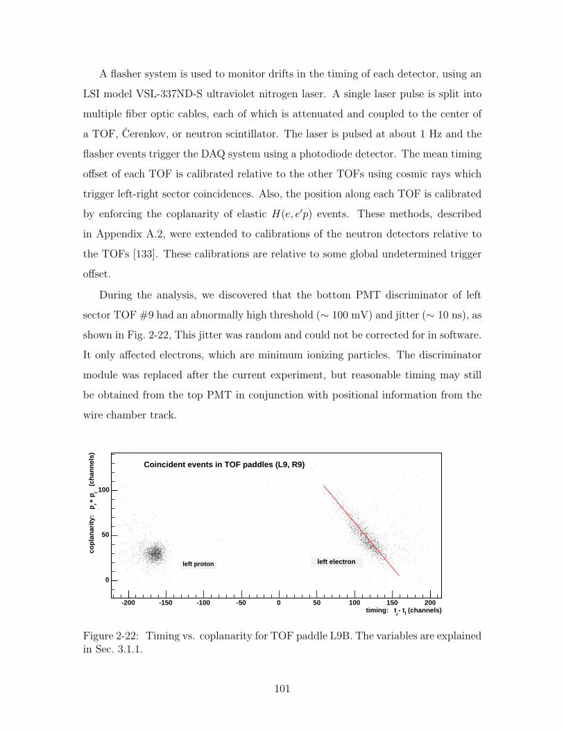
A flasher system is used to monitor drifts in the timing of each detector, using an

LSI model VSL-337ND-S ultraviolet nitrogen laser. A single laser pulse is split into

multiple fiber optic cables, each of which is attenuated and coupled to the center of

a TOF, Cerenkov, or neutron scintillator. The laser is pulsed at about 1 Hz and the

flasher events trigger the DAQ system using a photodiode detector. The mean timing

offset of each TOF is calibrated relative to the other TOFs using cosmic rays which

trigger left-right sector coincidences. Also, the position along each TOF is calibrated

by enforcing the coplanarity of elastic H(e, e′p) events. These methods, described

in Appendix A.2, were extended to calibrations of the neutron detectors relative to

the TOFs [133]. These calibrations are relative to some global undetermined trigger

offset.

During the analysis, we discovered that the bottom PMT discriminator of left

sector TOF #9 had an abnormally high threshold (∼ 100 mV) and jitter (∼ 10 ns), as

shown in Fig. 2-22, This jitter was random and could not be corrected for in software.

It only affected electrons, which are minimum ionizing particles. The discriminator

module was replaced after the current experiment, but reasonable timing may still

be obtained from the top PMT in conjunction with positional information from the

wire chamber track.

(channels)l- tr

timing: t-200 -150 -100 -50 0 50 100 150 200

(c

han

nel

s)l

+ p

rco

pla

nar

ity:

p

0

50

100

Coincident events in TOF paddles (L9, R9)

left proton left electron

Figure 2-22: Timing vs. coplanarity for TOF paddle L9B. The variables are explainedin Sec. 3.1.1.

101

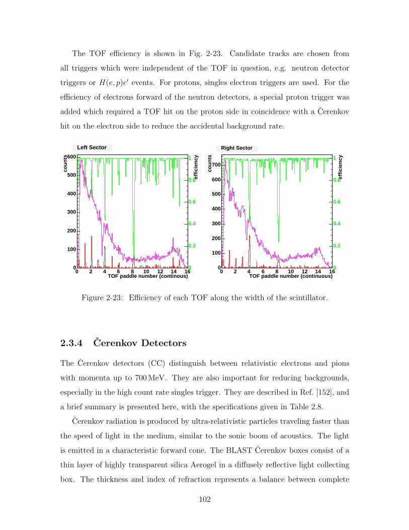
The TOF efficiency is shown in Fig. 2-23. Candidate tracks are chosen from

all triggers which were independent of the TOF in question, e.g. neutron detector

triggers or H(e, p)e′ events. For protons, singles electron triggers are used. For the

efficiency of electrons forward of the neutron detectors, a special proton trigger was

added which required a TOF hit on the proton side in coincidence with a Cerenkov

hit on the electron side to reduce the accidental background rate.

TOF paddle number (continous)0 2 4 6 8 10 12 14 16

cou

nts

0

100

200

300

400

500

600

Left Sector

effi

cien

cy

0

0.2

0.4

0.6

0.8

1

TOF paddle number (continuous)0 2 4 6 8 10 12 14 16

cou

nts

0

100

200

300

400

500

600

700

Right Sector

effi

cien

cy

0

0.2

0.4

0.6

0.8

1

Figure 2-23: Efficiency of each TOF along the width of the scintillator.

2.3.4 Cerenkov Detectors

The Cerenkov detectors (CC) distinguish between relativistic electrons and pions

with momenta up to 700 MeV. They are also important for reducing backgrounds,

especially in the high count rate singles trigger. They are described in Ref. [152], and

a brief summary is presented here, with the specifications given in Table 2.8.

Cerenkov radiation is produced by ultra-relativistic particles traveling faster than

the speed of light in the medium, similar to the sonic boom of acoustics. The light

is emitted in a characteristic forward cone. The BLAST Cerenkov boxes consist of a

thin layer of highly transparent silica Aerogel in a diffusely reflective light collecting

box. The thickness and index of refraction represents a balance between complete

102

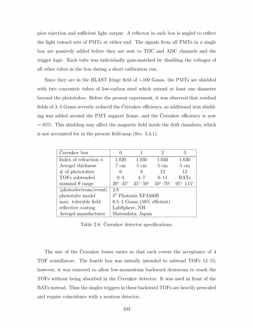
pion rejection and sufficient light output. A reflector in each box is angled to reflect

the light toward sets of PMTs at either end. The signals from all PMTs in a single

box are passively added before they are sent to TDC and ADC channels and the

trigger logic. Each tube was individually gain-matched by disabling the voltages of

all other tubes in the box during a short calibration run.

Since they are in the BLAST fringe field of ∼100 Gauss, the PMTs are shielded

with two concentric tubes of low-carbon steel which extend at least one diameter

beyond the phototubes. Before the present experiment, it was observed that residual

fields of 3–5 Gauss severely reduced the Cerenkov efficiency, so additional iron shield-

ing was added around the PMT support frame, and the Cerenkov efficiency is now

∼ 85%. This shielding may affect the magnetic field inside the drift chambers, which

is not accounted for in the present field-map (Sec. 3.4.1).

Cerenkov box 0 1 2 3

Index of refraction n 1.020 1.030 1.030 1.030Aerogel thickness 7 cm 5 cm 5 cm 5 cm# of phototubes 6 8 12 12TOFs subtended 0–3 4–7 8–11 BATsnominal θ range 20–35 35–50 50–70 95–115

〈photoelectrons/event〉 2.8phototube model 5′′ Photonis XP4500Bmax. tolerable field 0.5–1 Gauss (50% efficient)reflective coating LabSphere, NHAerogel manufacturer Matsushita, Japan

Table 2.8: Cerenkov detector specifications.

The size of the Cerenkov boxes varies so that each covers the acceptance of 4

TOF scintillators. The fourth box was initially intended to subtend TOFs 12–15;

however, it was removed to allow low-momentum backward deuterons to reach the

TOFs without being absorbed in the Cerenkov detector. It was used in front of the

BATs instead. Thus the singles triggers in these backward TOFs are heavily prescaled

and require coincidence with a neutron detector.

103

2.4 Electronics and Software

2.4.1 Trigger

The BLAST trigger is versatile, programmable, and can accept the multiple physics

channels present in a large-angle spectrometer. The trigger software and design were

developed in conjunction with JLab Hall A and tested there prior to their use in

BLAST. Software improvements for BLAST were also sent back to Hall A. Figure 2-

24 is a schematic of the electronic components. The raw signals from each detector

are split off to the ADC channels, and to the timing components (discriminators,

programmable delays, mean-timers). The latter signal is sent to the TDC modules

and also to input bits of the trigger logic. All except for the 4 most forward TOFs are

paired, and the entire Cerenkov and neutron sub-detectors are each combined into

one input bit per sector. The programmable logic is implemented with LeCroy 2373

Memory Lookup Units (MLUs). The MLU is a real-time look up table with multiple

output bits for each combination of input bits (signals). There are too many input

signals for one 16-bit MLU so the logic is split into left and right sector MLUs. The

output bits of both sector MLUs are combined in the cross MLU, which defines the

eight separate trigger types listed in Table 2.11. Each trigger type can be individually

prescaled. Multiple physics channels can be assigned to the same trigger bit, but they

will have the same prescale factor.

There is a second level wire chamber trigger which is too slow to start the TDCs

and ADCs, but instead accepts or rejects readout. This reduces the deadtime of noise

events from 835 µs for read out down to 5 µs for a start trigger and fast clear. The

second-level trigger, implemented in a custom designed electronics module, requires

at least one hit in each of the three wire chambers in one sector. Midway through

our experiment, the DAQ deadtime was further decreased by enhancing the logic to

require the above wire chamber pattern in each sector with a TOF hit.

The trigger distribution, common strobe, prescaling, external inhibit, internal

busy inhibit, event synchronization, and up to three levels of triggers are all man-

aged by the trigger supervisor (TS) module. The TS was developed at JLab and is

104

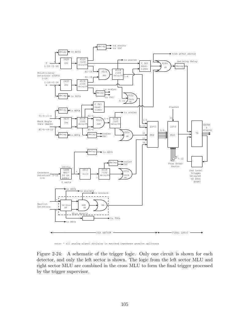
CFD

CFD

AND

Back AngleTOFs (BATS)

ScintillatorDetectors (TOFs) 1-16

T1-16->1-16

1-16->1-16 B

PER SECTOR

GATES &STARTS

MLU

FINAL LOGIC

delay/FO

delay/FO

to scalerto TDC

3420

3420

4518 /100

4518 /100

4516A1-16

B1-16

AND

4516 CFD

delay/FO delay/FO

3420 4518 /100

4518 /100

A1-4

B1-4

T1-4->1-4

B1-4->9-12

1-4

2373

MLU

2373

From Other Sector

delay/FO

4518 /100

OR

4564

1-4

5-16

Retiming Delay

Delay

to ADCs

to ADCs

to ADCs

to ADCs

PAIROR

4532

OR

4564

to scaler

Flasher

1-4

5-10

11

12

16

1-6

7-12

15

C 561mean-timer

delay

delay

*

*

*

*

note: * all analog signal division in matched impedance passive splitters

LE Disc X8

to ADCs

to ADCs

*

*

AND X8

OR

to scalers

Miro Module

TS

to scalers

to TDCs

NeutronDetectors

2nd Level Trigger(diagram on next page)

from other sector

scalerTDC

delay

C 561mean-timer

to scaler

to TDC

discrCerenkovDetectors 1-4

3412

1-12 delay/FO

4518 /100

to ADCs

CAEN N40724 chadder

4 units

2X10ns

delay

PAIROR

4532

scalerTDC

delay

*

to scaler

delay

delay

delay

delay

Figure 2-24: A schematic of the trigger logic. Only one circuit is shown for eachdetector, and only the left sector is shown. The logic from the left sector MLU andright sector MLU are combined in the cross MLU to form the final trigger processedby the trigger supervisor.

105

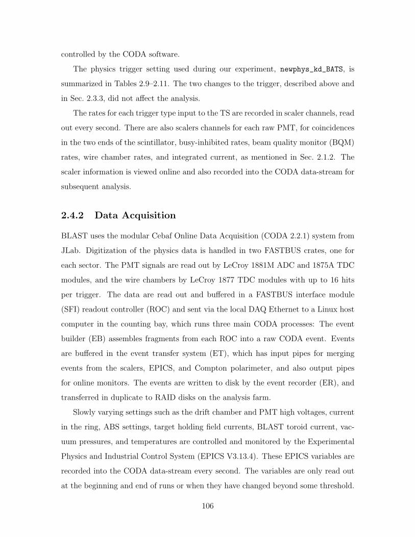
controlled by the CODA software.

The physics trigger setting used during our experiment, newphys_kd_BATS, is

summarized in Tables 2.9–2.11. The two changes to the trigger, described above and

in Sec. 2.3.3, did not affect the analysis.

The rates for each trigger type input to the TS are recorded in scaler channels, read

out every second. There are also scalers channels for each raw PMT, for coincidences

in the two ends of the scintillator, busy-inhibited rates, beam quality monitor (BQM)

rates, wire chamber rates, and integrated current, as mentioned in Sec. 2.1.2. The

scaler information is viewed online and also recorded into the CODA data-stream for

subsequent analysis.

2.4.2 Data Acquisition

BLAST uses the modular Cebaf Online Data Acquisition (CODA 2.2.1) system from

JLab. Digitization of the physics data is handled in two FASTBUS crates, one for

each sector. The PMT signals are read out by LeCroy 1881M ADC and 1875A TDC

modules, and the wire chambers by LeCroy 1877 TDC modules with up to 16 hits

per trigger. The data are read out and buffered in a FASTBUS interface module

(SFI) readout controller (ROC) and sent via the local DAQ Ethernet to a Linux host

computer in the counting bay, which runs three main CODA processes: The event

builder (EB) assembles fragments from each ROC into a raw CODA event. Events

are buffered in the event transfer system (ET), which has input pipes for merging

events from the scalers, EPICS, and Compton polarimeter, and also output pipes

for online monitors. The events are written to disk by the event recorder (ER), and

transferred in duplicate to RAID disks on the analysis farm.

Slowly varying settings such as the drift chamber and PMT high voltages, current

in the ring, ABS settings, target holding field currents, BLAST toroid current, vac-

uum pressures, and temperatures are controlled and monitored by the Experimental

Physics and Industrial Control System (EPICS V3.13.4). These EPICS variables are

recorded into the CODA data-stream every second. The variables are only read out

at the beginning and end of runs or when they have changed beyond some threshold.

106

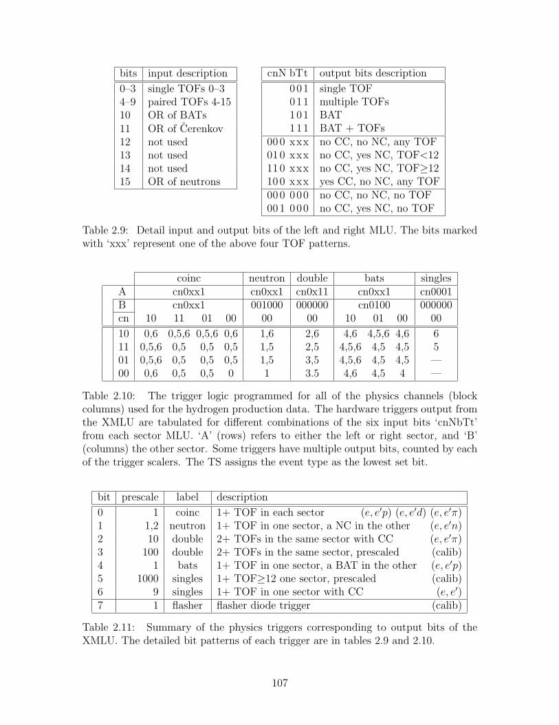
bits input description

0–3 single TOFs 0–34–9 paired TOFs 4-1510 OR of BATs11 OR of Cerenkov12 not used13 not used14 not used15 OR of neutrons

cnN bTt output bits description

001 single TOF011 multiple TOFs101 BAT111 BAT + TOFs

00 0 xxx no CC, no NC, any TOF010 xxx no CC, yes NC, TOF<1211 0 xxx no CC, yes NC, TOF≥1210 0 xxx yes CC, no NC, any TOF000 000 no CC, no NC, no TOF001 000 no CC, yes NC, no TOF

Table 2.9: Detail input and output bits of the left and right MLU. The bits markedwith ‘xxx’ represent one of the above four TOF patterns.

coinc neutron double bats singlesA cn0xx1 cn0xx1 cn0x11 cn0xx1 cn0001B cn0xx1 001000 000000 cn0100 000000cn 10 11 01 00 00 00 10 01 00 00

10 0,6 0,5,6 0,5,6 0,6 1,6 2,6 4,6 4,5,6 4,6 611 0,5,6 0,5 0,5 0,5 1,5 2,5 4,5,6 4,5 4,5 501 0,5,6 0,5 0,5 0,5 1,5 3,5 4,5,6 4,5 4,5 —00 0,6 0,5 0,5 0 1 3.5 4,6 4,5 4 —

Table 2.10: The trigger logic programmed for all of the physics channels (blockcolumns) used for the hydrogen production data. The hardware triggers output fromthe XMLU are tabulated for different combinations of the six input bits ‘cnNbTt’from each sector MLU. ‘A’ (rows) refers to either the left or right sector, and ‘B’(columns) the other sector. Some triggers have multiple output bits, counted by eachof the trigger scalers. The TS assigns the event type as the lowest set bit.

bit prescale label description

0 1 coinc 1+ TOF in each sector (e, e′p) (e, e′d) (e, e′π)1 1,2 neutron 1+ TOF in one sector, a NC in the other (e, e′n)2 10 double 2+ TOFs in the same sector with CC (e, e′π)3 100 double 2+ TOFs in the same sector, prescaled (calib)4 1 bats 1+ TOF in one sector, a BAT in the other (e, e′p)5 1000 singles 1+ TOF≥12 one sector, prescaled (calib)6 9 singles 1+ TOF in one sector with CC (e, e′)7 1 flasher flasher diode trigger (calib)

Table 2.11: Summary of the physics triggers corresponding to output bits of theXMLU. The detailed bit patterns of each trigger are in tables 2.9 and 2.10.

107

Physics events must be sandwiched by both EPICS and scalers events to be valid.

All events are timestamped by the ROCs, which are synchronized to the CODA host

computer dblast07 every minute by a fast Network Time Protocol (NTP) with 40

time samples. The overall synchronization is better than 10 ms, typically 5 ms. The

same protocol is used to synchronize the scaler readout times. The EPICS server and

dblast7 are synchronized using a common server at bates (locus).

Each CODA run is automatically logged in the electronic logbook (elog), which

was modified from the Jefferson Lab Hall A logbook to include a MySQL database

of entries. Run parameters such as the run number, target gas, holding field, data

quality, and trigger, electronics, epics and scaler maps are recorded in a searchable

RUN table in the database. The logbook also has manual entries including special

shift summary report forms.

2.4.3 Online Monitor

There were several online monitors to ensure data quality. All EPICS variables were

guarded by the AlarmHandler program. The DataAlarm script checked every 10

seconds that physics, scalers, EPICS, and Compton events in the CODA data-stream

were being recorded to disk. The raw rates were also monitored with online scalers,

including the BQM and wire chamber scalers, which were used to improve the beam

tune and reduce backgrounds.

The TDC and ADC spectra from each detector were monitored directly from

the CODA ET data-stream with the program onlineGui. This root-based graphical

monitor is based on the reconstruction library, and also histograms wire chamber

track parameters p, θ, φ, z, q, W , and pX for a subset of the events. In addition, the

data were fully reconstructed into ntuples by the offline farm within about 8 hours.

These ntuples were analyzed daily for preliminary physics results, including the target

polarization.

The event display utility nsed has been particularly useful for visually inspecting

the quality of online data and for debugging the reconstruction code. It is used for

verification of the electronics map by making sure all hits in a track line up. It

108

is based on the same reconstruction library the ntuples are generated from. It can

display events selected by a graphical cut in an arbitrary histogram, and mark the

current event with a triangle in all histograms that are currently being displayed, as

illustrated in Fig. 2-25.

(deg)Rθ20 30 40 50 60 70 80

(d

eg)

Lθ

20

30

40

50

60

70

80twl:twr qwl*qwr==-1

Figure 2-25: Integration of online display (NSED) with ROOT analysis package.

2.4.4 Reconstruction Library

All reconstruction software (lrn, lrd, nsed, onlineGui, analysis scripts) is based

on the common library, BlastLib2, which provides uniformity and efficiency. Recon-

structed ntuple values can be verified in the online display, and all programs recognize

the same options and settings. The open-source library is written in C++ using stan-

dard UNIX utilities autoconf, make, and gcc. The current version v3.4.4 contains

37500 lines of code and is maintained in the BLAST CVS repository. It is built on

the framework of ROOT and uses many of its basic features, listed in Table 2.12.

The key functions of the library and its corresponding classes are listed in Ta-

ble 2.13. The library decodes raw CODA data-files into detector hits using an elec-

tronics map configuration file, which maps the ROC addresses, crate slots, and module

channels into physical detector components. The data for each individual detector are

109

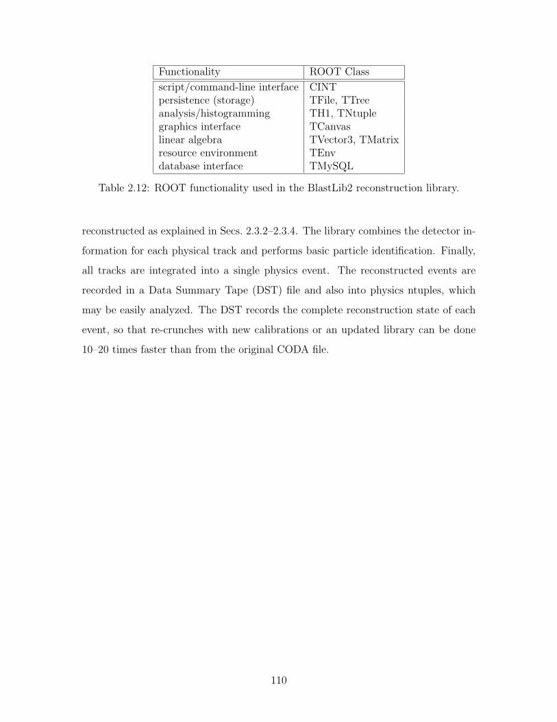
Functionality ROOT Class

script/command-line interface CINTpersistence (storage) TFile, TTreeanalysis/histogramming TH1, TNtuplegraphics interface TCanvaslinear algebra TVector3, TMatrixresource environment TEnvdatabase interface TMySQL

Table 2.12: ROOT functionality used in the BlastLib2 reconstruction library.

reconstructed as explained in Secs. 2.3.2–2.3.4. The library combines the detector in-

formation for each physical track and performs basic particle identification. Finally,

all tracks are integrated into a single physics event. The reconstructed events are

recorded in a Data Summary Tape (DST) file and also into physics ntuples, which

may be easily analyzed. The DST records the complete reconstruction state of each

event, so that re-crunches with new calibrations or an updated library can be done

10–20 times faster than from the original CODA file.

110

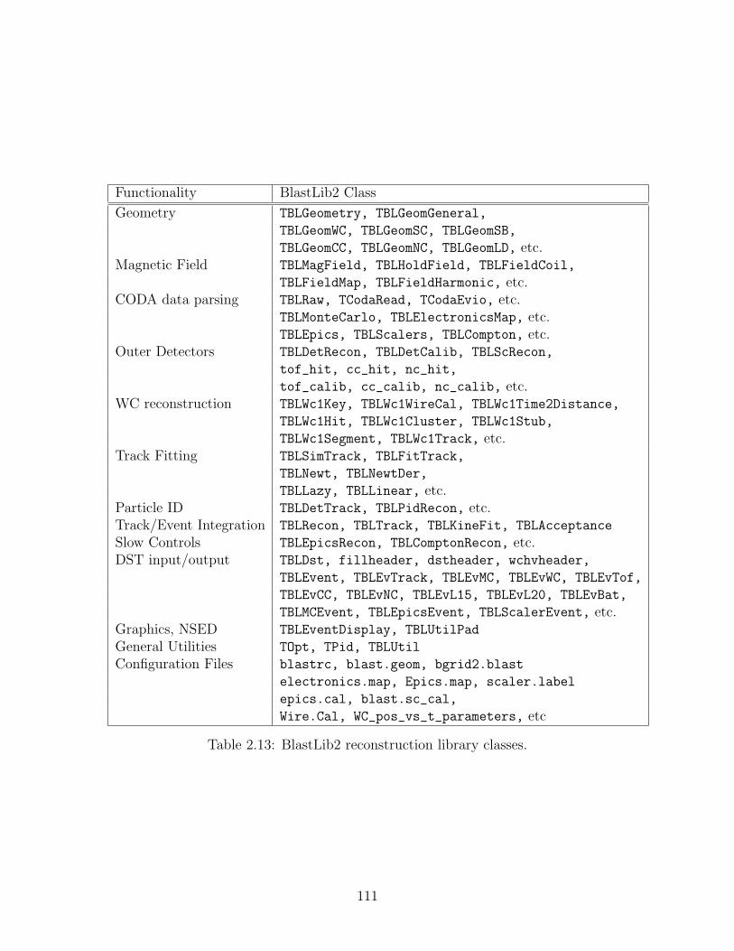
Functionality BlastLib2 Class

Geometry TBLGeometry, TBLGeomGeneral,

TBLGeomWC, TBLGeomSC, TBLGeomSB,

TBLGeomCC, TBLGeomNC, TBLGeomLD, etc.Magnetic Field TBLMagField, TBLHoldField, TBLFieldCoil,

TBLFieldMap, TBLFieldHarmonic, etc.CODA data parsing TBLRaw, TCodaRead, TCodaEvio, etc.

TBLMonteCarlo, TBLElectronicsMap, etc.TBLEpics, TBLScalers, TBLCompton, etc.

Outer Detectors TBLDetRecon, TBLDetCalib, TBLScRecon,

tof_hit, cc_hit, nc_hit,

tof_calib, cc_calib, nc_calib, etc.WC reconstruction TBLWc1Key, TBLWc1WireCal, TBLWc1Time2Distance,

TBLWc1Hit, TBLWc1Cluster, TBLWc1Stub,

TBLWc1Segment, TBLWc1Track, etc.Track Fitting TBLSimTrack, TBLFitTrack,

TBLNewt, TBLNewtDer,

TBLLazy, TBLLinear, etc.Particle ID TBLDetTrack, TBLPidRecon, etc.Track/Event Integration TBLRecon, TBLTrack, TBLKineFit, TBLAcceptance

Slow Controls TBLEpicsRecon, TBLComptonRecon, etc.DST input/output TBLDst, fillheader, dstheader, wchvheader,

TBLEvent, TBLEvTrack, TBLEvMC, TBLEvWC, TBLEvTof,

TBLEvCC, TBLEvNC, TBLEvL15, TBLEvL20, TBLEvBat,

TBLMCEvent, TBLEpicsEvent, TBLScalerEvent, etc.Graphics, NSED TBLEventDisplay, TBLUtilPad

General Utilities TOpt, TPid, TBLUtil

Configuration Files blastrc, blast.geom, bgrid2.blast

electronics.map, Epics.map, scaler.label

epics.cal, blast.sc_cal,

Wire.Cal, WC_pos_vs_t_parameters, etc

Table 2.13: BlastLib2 reconstruction library classes.

111

112

Chapter 3

Data Analysis

Data for this experiment were taken during three run periods, listed in Table 3.1. The

first run was taken with the BLAST magnetic field reversed (electrons out-bending)

to extend the acceptance to lower Q2. The rates are higher at lower Q2, allowing an

accurate measurement of the target polarization in less time. Data were taken with

the ABS target. Between the second and third run periods, the ABS performance was

greatly improved, which affected both the target thickness and polarization. Also, the

40 cm long cell was replaced with a 60 cm long cell (cell #3) of the same diameter. As

a result the third run period yielded over 13 times the effective statistics of the first

two run periods combined. The majority of the data in the third run were taken with

the magnetic holding field oriented at 47 with respect to the beam line. Between the

second and third run periods, deuterium data with 450 kC of accumulated charge were

also taken, and even more deuterium data are being taken in the 2005 deuterium run.

One can also extract the proton form factor ratio from quasi-elastic scattering from

deuterium, although it is complicated by nuclear effects such the deuteron structure

and final state interactions (FSI). However, for the scope of this thesis, only the results

of the hydrogen data from run 3 with the holding field at 47 are presented.

113

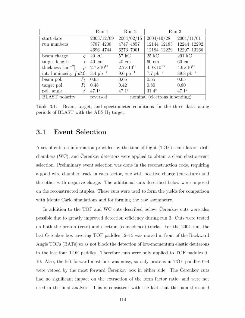
Run 1 Run 2 Run 3

start date 2003/12/09 2004/02/15 2004/10/28 2004/11/01run numbers 3787–4208 4747–4857 12144–12183 12244–12292

4696–4744 6273–7001 12184–12229 12297–13266beam charge q 20 kC 57 kC 25 kC 291 kCtarget length l 40 cm 40 cm 60 cm 60 cmthickness [cm−2] ρ 2.7×1013 2.7×1013 4.9×1013 4.9×1013

int. luminosity∫

dtL 3.4 pb−1 9.6 pb−1 7.7 pb−1 89.8 pb−1

beam pol. Pb 0.65 0.65 0.65 0.65target pol. Pt 0.48 0.42 0.80 0.80pol. angle β 47.1 47.1 31.4 47.1

BLAST polarity reversed nominal (electrons inbending)

Table 3.1: Beam, target, and spectrometer conditions for the three data-takingperiods of BLAST with the ABS H2 target.

3.1 Event Selection

A set of cuts on information provided by the time-of-flight (TOF) scintillators, drift

chambers (WC), and Cerenkov detectors were applied to obtain a clean elastic event

selection. Preliminary event selection was done in the reconstruction code, requiring

a good wire chamber track in each sector, one with positive charge (curvature) and

the other with negative charge. The additional cuts described below were imposed

on the reconstructed ntuples. These cuts were used to form the yields for comparison

with Monte Carlo simulations and for forming the raw asymmetry.

In addition to the TOF and WC cuts described below, Cerenkov cuts were also

possible due to greatly improved detection efficiency during run 3. Cuts were tested

on both the proton (veto) and electron (coincidence) tracks. For the 2004 run, the

last Cerenkov box covering TOF paddles 12–15 was moved in front of the Backward

Angle TOFs (BATs) so as not block the detection of low-momentum elastic deuterons

in the last four TOF paddles. Therefore cuts were only applied to TOF paddles 0–

10. Also, the left forward-most box was noisy, so only protons in TOF paddles 0–4

were vetoed by the most forward Cerenkov box in either side. The Cerenkov cuts

had no significant impact on the extraction of the form factor ratio, and were not

used in the final analysis. This is consistent with the fact that the pion threshold

114

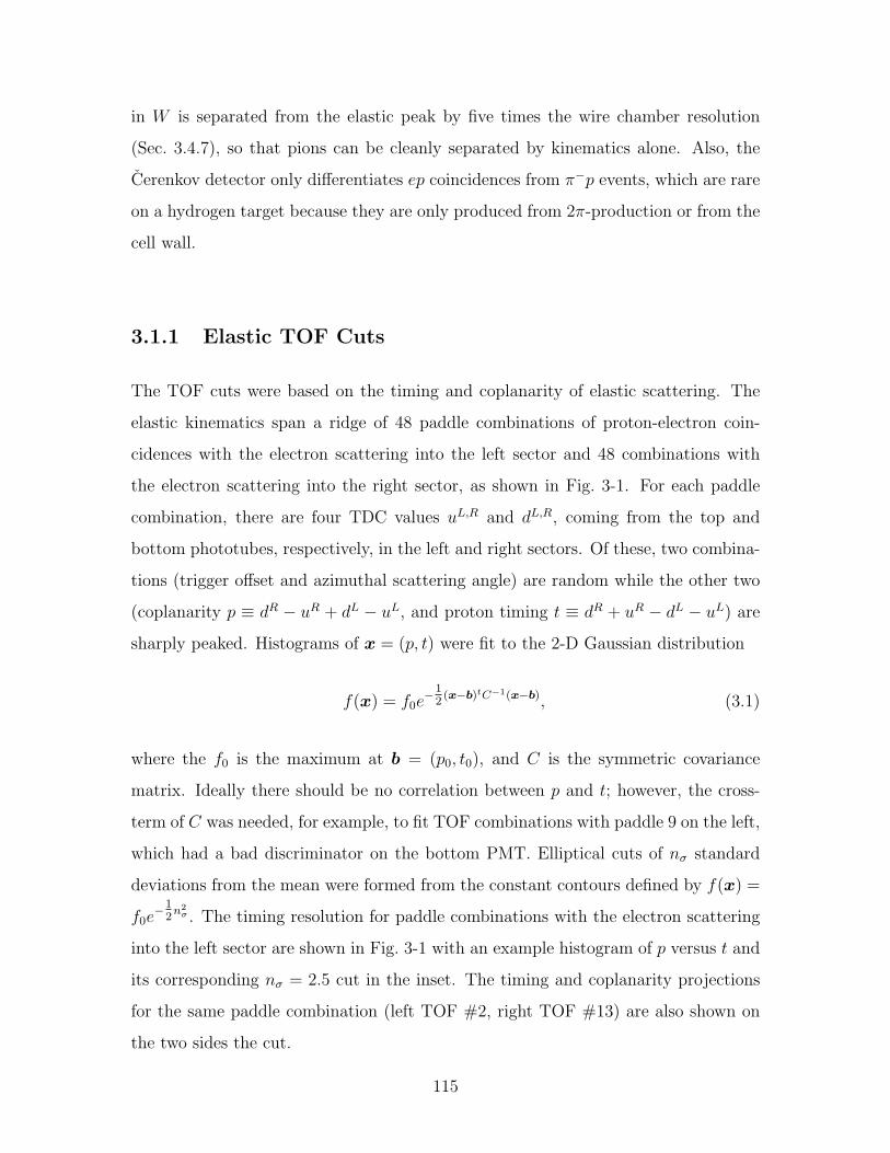
in W is separated from the elastic peak by five times the wire chamber resolution

(Sec. 3.4.7), so that pions can be cleanly separated by kinematics alone. Also, the

Cerenkov detector only differentiates ep coincidences from π−p events, which are rare

on a hydrogen target because they are only produced from 2π-production or from the

cell wall.

3.1.1 Elastic TOF Cuts

The TOF cuts were based on the timing and coplanarity of elastic scattering. The

elastic kinematics span a ridge of 48 paddle combinations of proton-electron coin-

cidences with the electron scattering into the left sector and 48 combinations with

the electron scattering into the right sector, as shown in Fig. 3-1. For each paddle

combination, there are four TDC values uL,R and dL,R, coming from the top and

bottom phototubes, respectively, in the left and right sectors. Of these, two combina-

tions (trigger offset and azimuthal scattering angle) are random while the other two

(coplanarity p ≡ dR − uR + dL − uL, and proton timing t ≡ dR + uR − dL − uL) are

sharply peaked. Histograms of x = (p, t) were fit to the 2-D Gaussian distribution

f(x) = f0e−1

2(x−b)tC−1(x−b), (3.1)

where the f0 is the maximum at b = (p0, t0), and C is the symmetric covariance

matrix. Ideally there should be no correlation between p and t; however, the cross-

term of C was needed, for example, to fit TOF combinations with paddle 9 on the left,

which had a bad discriminator on the bottom PMT. Elliptical cuts of nσ standard

deviations from the mean were formed from the constant contours defined by f(x) =

f0e−1

2n2

σ . The timing resolution for paddle combinations with the electron scattering

into the left sector are shown in Fig. 3-1 with an example histogram of p versus t and

its corresponding nσ = 2.5 cut in the inset. The timing and coplanarity projections

for the same paddle combination (left TOF #2, right TOF #13) are also shown on

the two sides the cut.

115

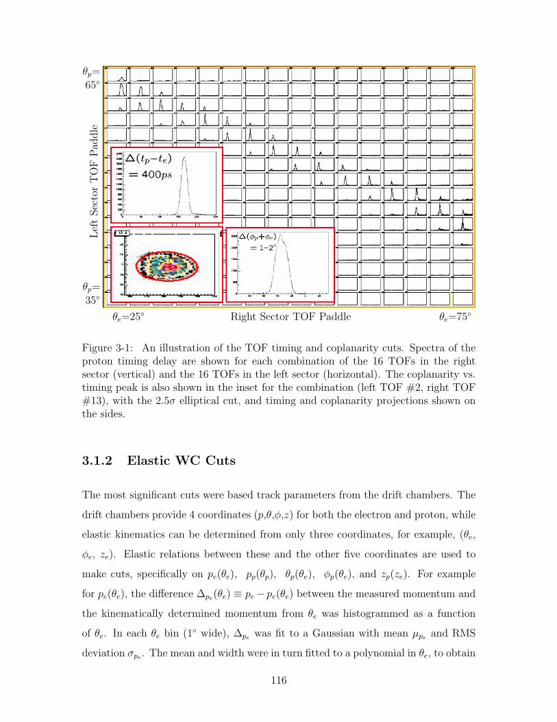
θp=65

θp=35

θe=25 θe=75Right Sector TOF Paddle

Lef

tSec

tor

TO

FPad

dle

Figure 3-1: An illustration of the TOF timing and coplanarity cuts. Spectra of theproton timing delay are shown for each combination of the 16 TOFs in the rightsector (vertical) and the 16 TOFs in the left sector (horizontal). The coplanarity vs.timing peak is also shown in the inset for the combination (left TOF #2, right TOF#13), with the 2.5σ elliptical cut, and timing and coplanarity projections shown onthe sides.

3.1.2 Elastic WC Cuts

The most significant cuts were based track parameters from the drift chambers. The

drift chambers provide 4 coordinates (p,θ,φ,z) for both the electron and proton, while

elastic kinematics can be determined from only three coordinates, for example, (θe,

φe, ze). Elastic relations between these and the other five coordinates are used to

make cuts, specifically on pe(θe), pp(θp), θp(θe), φp(θe), and zp(ze). For example

for pe(θe), the difference ∆pe(θe) ≡ pe− pe(θe) between the measured momentum and

the kinematically determined momentum from θe was histogrammed as a function

of θe. In each θe bin (1 wide), ∆pe was fit to a Gaussian with mean µpe and RMS

deviation σpe . The mean and width were in turn fitted to a polynomial in θe, to obtain

116

the momentum offset µpe(θe) ≡ 〈∆pe〉 and the relative deviation χp(θe) ≡ (∆pe −

µpe)/σpe of each event from elastic kinematics, with the associated cut |χp| < nσ. We

investigated the dependence of the asymmetry and polarization on the width of the

cut nσ, and found very little variation. We chose to use independent 2.5σ cuts on

each of the five redundant wire chamber variables. The distributions of ∆ for each

relation are shown in Fig. 3-2 with curves for the average, 1σ resolution, and the 2.5σ

cuts.

The cut on pe(θe) is equivalent to a cut on invariant mass W 2 ≡ (q + p2)2 =

M2 + 2Mν −Q2, except that it varies along with the width of the peak as a function

of θe. For radiative corrections (Sec. 3.2.3), it was necessary to use a cut on inelasticity

v = W 2 − M2. In order to obtain a clean cut on W , the electron momentum was

corrected by the offset −µpe . Likewise, the three cuts on pp(θp), θp(θe), φp(θe) are

equivalent to cuts on the missing 4-momentum pX ≡ k1−k2 + p1−p2 which has three

independent components when constrained by W . In elastic scattering pX should be

zero. The invariant mass (W ) and missing mass squared (M2X ≡ p2

X) spectra are

shown in Fig. 3-3. After the above corrections, pX is centered exactly about the

origin. The widths of the two components of the scattering plane δpxX = 27 MeV and

δpzX = 29 MeV are much wider than δpy

X = 6.7 MeV due their stronger dependence

on the reconstructed momentum resolution. Also, the former two are smeared by the

s- and p-peaks of the radiative tail in the scattering plane (Fig. 1-2b,c). The final

cut on zp(ze) is not an elastic cut, but rather a cut on reconstruction. It reduces

accidental coincidences by ensuring that tracks originate from the same vertex.

Additional boundaries were imposed on the range of each variable. The electron

and proton angles were restricted to 23 < θe < 76, 28 < θp < 69, and −14 <

φ < 14 to reduce the effect of wire chamber mis-reconstruction, especially at forward

angles of the measured acceptance. A vertex cut of −20 cm < z < 20 cm was also

used. Even though data were taken with a 60 cm long target cell, the holding field

was only constant in the region of the cell included in the cut. However, the target is

thickest in the center and only 1/16th of the events are come from the last 10 cm at

either end of the target.

117

[deg]eθ30 40 50 60 70

) [G

eV

]eθ(

e -

pe

p

-0.15

-0.1

-0.05

0

0.05

0.1

0.15 Electron Momentum vs. Scattering Angle LEFT sector

[deg]eθ30 40 50 60 70

) [G

eV

]eθ(

e -

pe

p

-0.15

-0.1

-0.05

0

0.05

0.1

0.15 Electron Momentum vs. Scattering Angle RIGHT sector

[deg]pθ30 35 40 45 50 55 60 65

) [G

eV

]pθ(

p -

pp

p

-0.15

-0.1

-0.05

0

0.05

0.1

0.15Proton Momentum vs. Recoil Angle

[deg]pθ30 35 40 45 50 55 60 65

) [G

eV

]pθ(

p -

pp

p

-0.15

-0.1

-0.05

0

0.05

0.1

0.15Proton Momentum vs. Recoil Angle

[deg]eθ30 40 50 60 70

) [d

eg

]eθ(

pθ -

pθ

-1.5

-1

-0.5

0

0.5

1

1.5Proton Recoil Angle vs. Electron Scattering Angle

[deg]eθ30 40 50 60 70

) [d

eg

]eθ(

pθ -

pθ

-1.5

-1

-0.5

0

0.5

1

1.5Proton Recoil Angle vs. Electron Scattering Angle

[deg]e

φ-10 -5 0 5 10

) [d

eg

]eφ(

eφ -

pφ

-3

-2

-1

0

1

2

3Proton vs. Electron Azimuthal Angle (Coplanarity)

[deg]e

φ-10 -5 0 5 10

) [d

eg

]eφ(

eφ -

pφ

-3

-2

-1

0

1

2

3Proton vs. Electron Azimuthal Angle (Coplanarity)

(cm)ez-20 -15 -10 -5 0 5 10 15 20

) [c

m]

e(z

e -

zpz

-4

-2

0

2

4

Proton vs. Electron Vertex Position

(cm)ez-20 -15 -10 -5 0 5 10 15 20

) [c

m]

e(z

e -

zpz

-4

-2

0

2

4

Proton vs. Electron Vertex Position

Figure 3-2: Drift Chamber cuts based on the five overdetermined track parameters:pe, pp, θp, φp, and zp. Each plot is a histogram of the difference between one ofthese variables and the same, calculated from another track parameter using elastickinematics. The left [right] panels correspond to electrons scattering into the left[right] sector. For example, in the top left panel, the electron momentum pe in the leftsector is calculated as a function pe(θe) of its scattering angle θe, and the difference ishistogrammed against θe. The five curves correspond to fits to the average kinematiccorrection, and 1σ and 2.5σ resolution. The 2.5σ band was used for drift chambercuts.

118

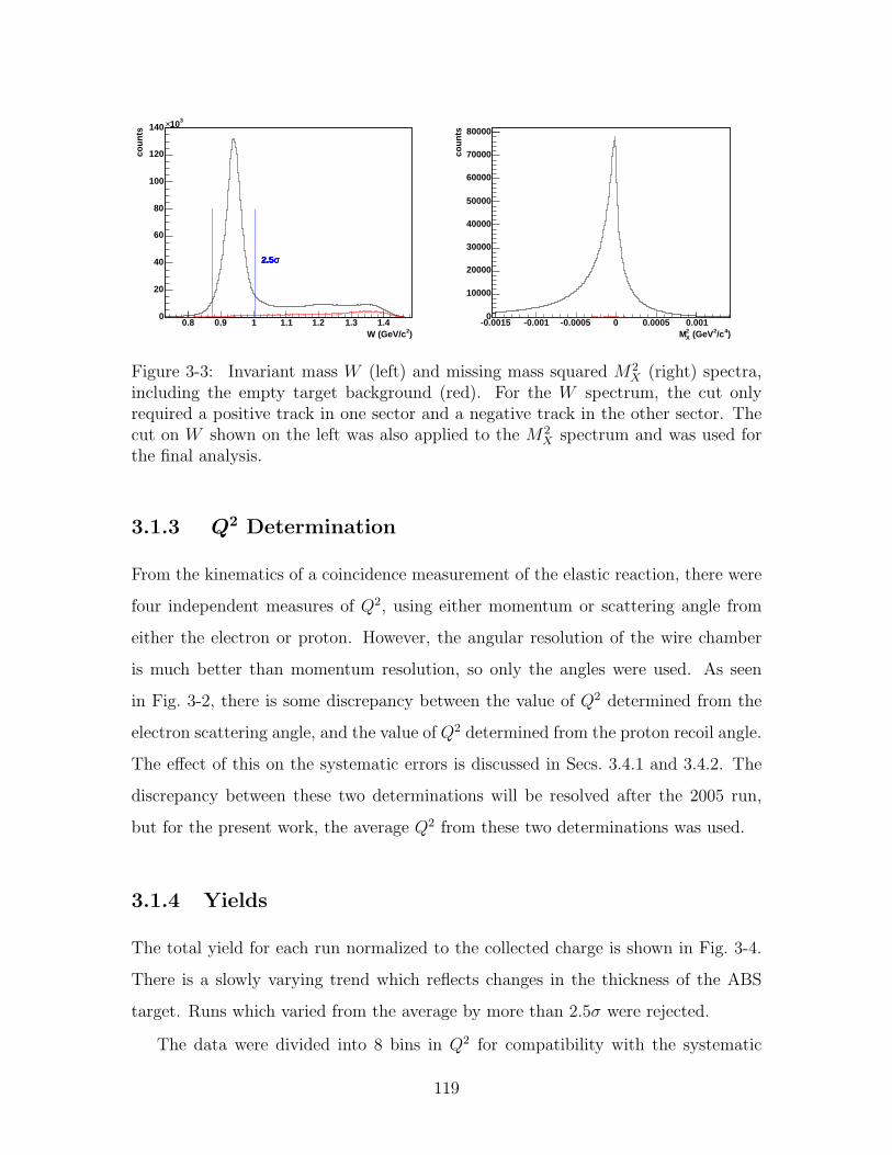
)2W (GeV/c0.8 0.9 1 1.1 1.2 1.3 1.4

cou

nts

0

20

40

60

80

100

120

140310×

σ2.5σ2.5σ2.5σ2.5

)4/c2 (GeV2XM

-0.0015 -0.001 -0.0005 0 0.0005 0.001

cou

nts

0

10000

20000

30000

40000

50000

60000

70000

80000

Figure 3-3: Invariant mass W (left) and missing mass squared M2X (right) spectra,

including the empty target background (red). For the W spectrum, the cut onlyrequired a positive track in one sector and a negative track in the other sector. Thecut on W shown on the left was also applied to the M2

X spectrum and was used forthe final analysis.

3.1.3 Q2 Determination

From the kinematics of a coincidence measurement of the elastic reaction, there were

four independent measures of Q2, using either momentum or scattering angle from

either the electron or proton. However, the angular resolution of the wire chamber

is much better than momentum resolution, so only the angles were used. As seen

in Fig. 3-2, there is some discrepancy between the value of Q2 determined from the

electron scattering angle, and the value of Q2 determined from the proton recoil angle.

The effect of this on the systematic errors is discussed in Secs. 3.4.1 and 3.4.2. The

discrepancy between these two determinations will be resolved after the 2005 run,

but for the present work, the average Q2 from these two determinations was used.

3.1.4 Yields

The total yield for each run normalized to the collected charge is shown in Fig. 3-4.

There is a slowly varying trend which reflects changes in the thickness of the ABS

target. Runs which varied from the average by more than 2.5σ were rejected.

The data were divided into 8 bins in Q2 for compatibility with the systematic

119

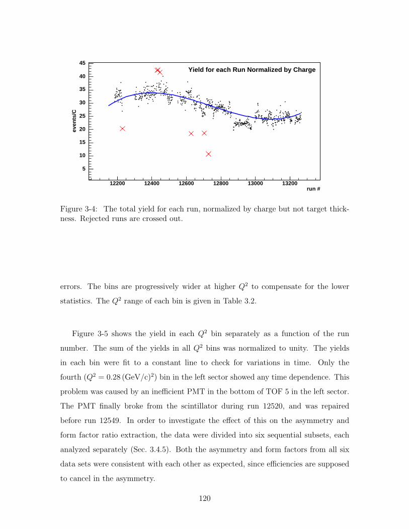
run #12200 12400 12600 12800 13000 13200

even

ts/C

5

10

15

20

25

30

35

40

45Yield for each Run Normalized by Charge

Figure 3-4: The total yield for each run, normalized by charge but not target thick-ness. Rejected runs are crossed out.

errors. The bins are progressively wider at higher Q2 to compensate for the lower

statistics. The Q2 range of each bin is given in Table 3.2.

Figure 3-5 shows the yield in each Q2 bin separately as a function of the run

number. The sum of the yields in all Q2 bins was normalized to unity. The yields

in each bin were fit to a constant line to check for variations in time. Only the

fourth (Q2 = 0.28 (GeV/c)2) bin in the left sector showed any time dependence. This

problem was caused by an inefficient PMT in the bottom of TOF 5 in the left sector.

The PMT finally broke from the scintillator during run 12520, and was repaired

before run 12549. In order to investigate the effect of this on the asymmetry and

form factor ratio extraction, the data were divided into six sequential subsets, each

analyzed separately (Sec. 3.4.5). Both the asymmetry and form factors from all six

data sets were consistent with each other as expected, since efficiencies are supposed

to cancel in the asymmetry.

120

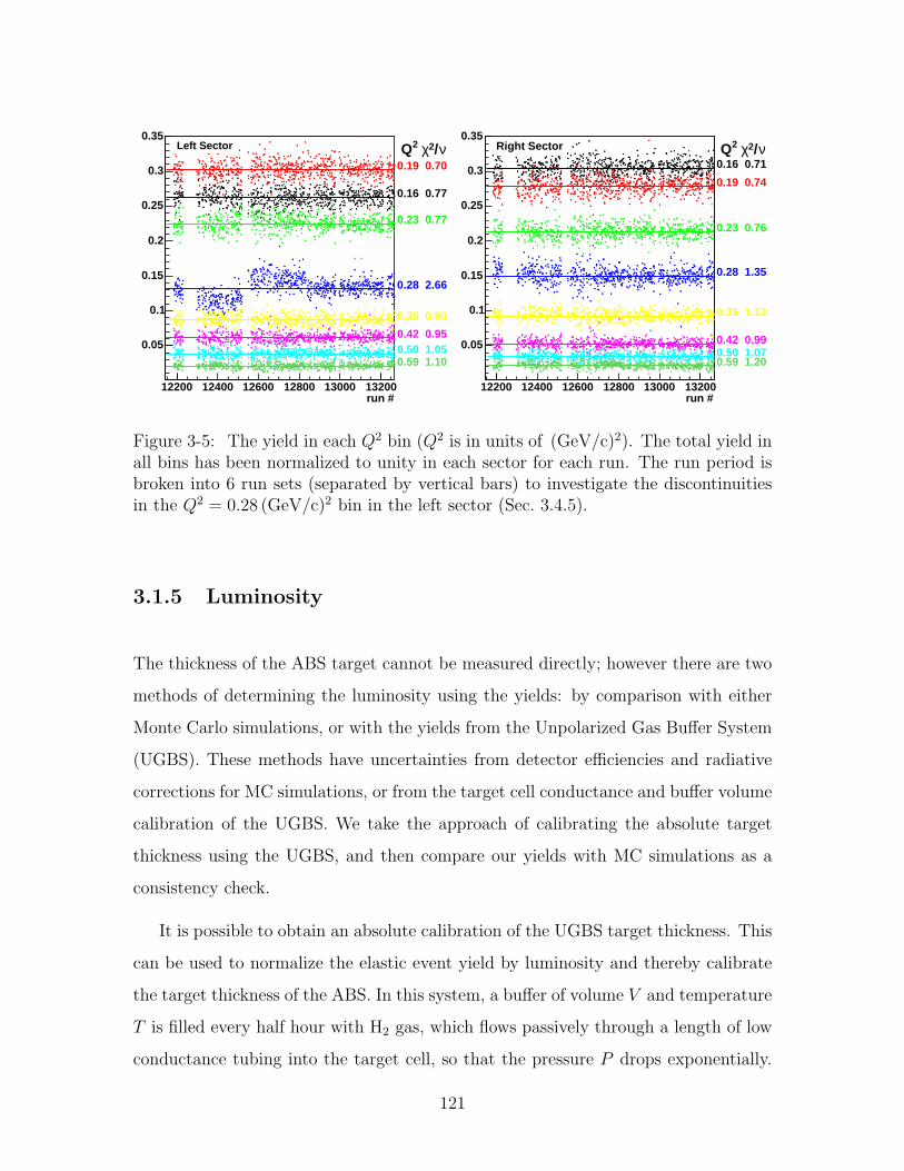
run #12200 12400 12600 12800 13000 13200

0.05

0.1

0.15

0.2

0.25

0.3

0.35

0.16 0.77

0.19 0.70

0.23 0.77

0.28 2.66

0.35 0.90

0.42 0.950.50 1.050.59 1.10

ν/2χ 2 QLeft Sector

run #12200 12400 12600 12800 13000 13200

0.05

0.1

0.15

0.2

0.25

0.3

0.35

0.16 0.71

0.19 0.74

0.23 0.76

0.28 1.35

0.35 1.13

0.42 0.990.50 1.070.59 1.20

ν/2χ 2 QRight Sector

Figure 3-5: The yield in each Q2 bin (Q2 is in units of (GeV/c)2). The total yield inall bins has been normalized to unity in each sector for each run. The run period isbroken into 6 run sets (separated by vertical bars) to investigate the discontinuitiesin the Q2 = 0.28 (GeV/c)2 bin in the left sector (Sec. 3.4.5).

3.1.5 Luminosity

The thickness of the ABS target cannot be measured directly; however there are two

methods of determining the luminosity using the yields: by comparison with either

Monte Carlo simulations, or with the yields from the Unpolarized Gas Buffer System

(UGBS). These methods have uncertainties from detector efficiencies and radiative

corrections for MC simulations, or from the target cell conductance and buffer volume

calibration of the UGBS. We take the approach of calibrating the absolute target

thickness using the UGBS, and then compare our yields with MC simulations as a

consistency check.

It is possible to obtain an absolute calibration of the UGBS target thickness. This

can be used to normalize the elastic event yield by luminosity and thereby calibrate

the target thickness of the ABS. In this system, a buffer of volume V and temperature

T is filled every half hour with H2 gas, which flows passively through a length of low

conductance tubing into the target cell, so that the pressure P drops exponentially.

121

The UGBS flow rate Φ can be accurately determined using the ideal gas law,

Φ = − V

kBT

dP

dt, (3.2)

where kB is the Boltzmann constant. In Fig. 3-6, the buffer pressure during runs

11870–11873 was fit to an exponential function of time to extract the average flow rate,

Φ = (8.11 ± 0.34)×1015 molecules/s. The density of gas in the cell was determined

from the conductance of the target cell as in Sec. 2.2.2. The target cell used for

production data for this experiment was a 60 cm long cylinder of diameter 1.5 cm,

connected in the center to a cylindrical feeding tube 15 cm long with a diameter of

1.27 cm. The unpolarized gas was injected into the center of the cell, and saw the

conductance of three cylinders in parallel with total conductance C = 8.03 L/s. The

areal density (target thickness) of the UGBS, ρ = 5.33×1013 cm−2, was obtained by

integration of the triangular density profile from z = −20 cm to z = 20 cm, the

region of the target used for the analysis of data. The integrated luminosity for these

UGBS runs was LUGBS =∫

dtρI/e = 0.163 pb−1, where∫

dtI = 4.91 kC was the

integrated beam current. Multiplying by the normalization YABS/YUGBS = 550.9, the

ABS integrated luminosity was LABS = 89.8 pb−1 for 294.2 kC of beam used in the

analysis of the form factor ratio, which corresponds to an average target thickness of

ρ = 4.89×1013 cm−2.

The error in the luminosity calibration is approximately 3%. The main errors

include the buffer pressure (2%) and the buffer volume (2%), which will be remeasured

to 1% accuracy at the end of the 2005 run. Other uncertainties include the calculation

of the conductance (which could be significant but at the moment is not known

conclusively), temperature variations (less than 0.3% because the hall temperature

was included in the calculation), and a systematic shift in the detector efficiency

between the UGBS and ABS runs, which were taken close together.

Using the luminosity from the UGBS, the normalized yield from the ABS target

was compared with MC simulations (Sec. 3.4.4) in Fig. 3-7. The Monte Carlo events

were generated from the elastic cross section with radiative corrections applied as

122

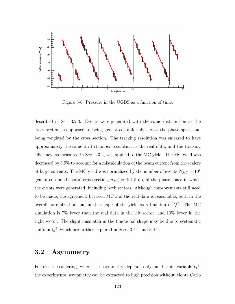
time (hours)0 0.5 1 1.5 2 2.5

bu

ffer

pre

ssu

re (

To

rr)

1.44

1.46

1.48

1.5

1.52

1.54

1.56

Figure 3-6: Pressure in the UGBS as a function of time.

described in Sec. 3.2.3. Events were generated with the same distribution as the

cross section, as opposed to being generated uniformly across the phase space and

being weighted by the cross section. The tracking resolution was smeared to have

approximately the same drift chamber resolution as the real data, and the tracking

efficiency, as measured in Sec. 2.3.2, was applied to the MC yield. The MC yield was

decreased by 3.5% to account for a miscalculation of the beam current from the scalers

at large currents. The MC yield was normalized by the number of events NMC = 107

generated and the total cross section, σMC = 161.5 nb, of the phase space in which

the events were generated, including both sectors. Although improvements still need

to be made, the agreement between MC and the real data is reasonable, both in the

overall normalization and in the shape of the yield as a function of Q2. The MC

simulation is 7% lower than the real data in the left sector, and 13% lower in the

right sector. The slight mismatch in the functional shape may be due to systematic

shifts in Q2, which are further explored in Secs. 3.4.1 and 3.4.2.

3.2 Asymmetry

For elastic scattering, where the asymmetry depends only on the bin variable Q2,

the experimental asymmetry can be extracted to high precision without Monte Carlo

123

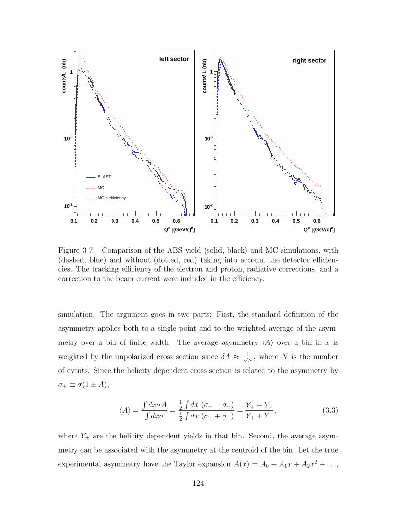
]2 [(GeV/c)2Q

0.1 0.2 0.3 0.4 0.5 0.6

cou

nts

/L (

nb

)

-210

-110

1

left sector

BLAST

MC

efficiency×MC

]2 [(GeV/c)2Q

0.1 0.2 0.3 0.4 0.5 0.6

cou

nts

/ L (

nb

)

-210

-110

1

right sector

Figure 3-7: Comparison of the ABS yield (solid, black) and MC simulations, with(dashed, blue) and without (dotted, red) taking into account the detector efficien-cies. The tracking efficiency of the electron and proton, radiative corrections, and acorrection to the beam current were included in the efficiency.

simulation. The argument goes in two parts: First, the standard definition of the

asymmetry applies both to a single point and to the weighted average of the asym-

metry over a bin of finite width. The average asymmetry 〈A〉 over a bin in x is

weighted by the unpolarized cross section since δA ≈ 1√N

, where N is the number

of events. Since the helicity dependent cross section is related to the asymmetry by

σ± ≡ σ(1± A),

〈A〉 =

∫dxσA∫dxσ

=12

∫dx (σ+ − σ−)

12

∫dx (σ+ + σ−)

=Y+ − Y−Y+ + Y−

, (3.3)

where Y± are the helicity dependent yields in that bin. Second, the average asym-

metry can be associated with the asymmetry at the centroid of the bin. Let the true

experimental asymmetry have the Taylor expansion A(x) = A0 + A1x + A2x2 + . . .,

124

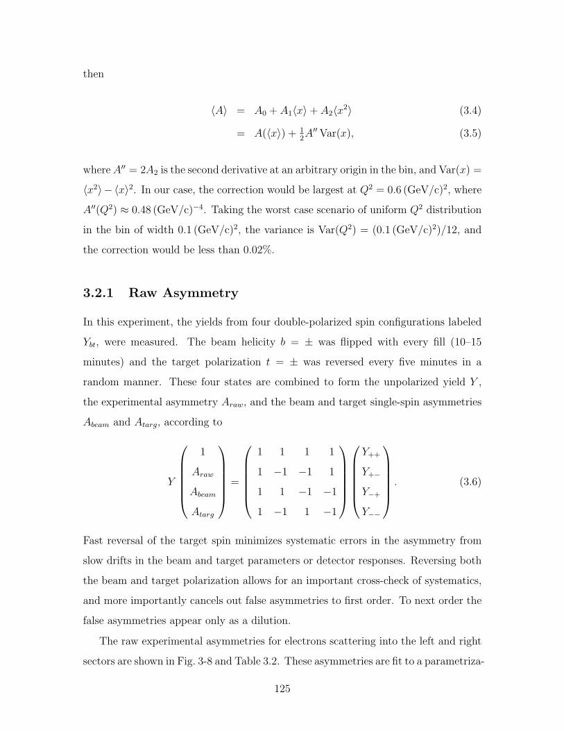
then

〈A〉 = A0 + A1〈x〉+ A2〈x2〉 (3.4)

= A(〈x〉) + 12A′′ Var(x), (3.5)

where A′′ = 2A2 is the second derivative at an arbitrary origin in the bin, and Var(x) =

〈x2〉− 〈x〉2. In our case, the correction would be largest at Q2 = 0.6 (GeV/c)2, where

A′′(Q2) ≈ 0.48 (GeV/c)−4. Taking the worst case scenario of uniform Q2 distribution

in the bin of width 0.1 (GeV/c)2, the variance is Var(Q2) = (0.1 (GeV/c)2)/12, and

the correction would be less than 0.02%.

3.2.1 Raw Asymmetry

In this experiment, the yields from four double-polarized spin configurations labeled

Ybt, were measured. The beam helicity b = ± was flipped with every fill (10–15

minutes) and the target polarization t = ± was reversed every five minutes in a

random manner. These four states are combined to form the unpolarized yield Y ,

the experimental asymmetry Araw, and the beam and target single-spin asymmetries

Abeam and Atarg, according to

Y

1

Araw

Abeam

Atarg

=

1 1 1 1

1 −1 −1 1

1 1 −1 −1

1 −1 1 −1

Y++

Y+−

Y−+

Y−−

. (3.6)

Fast reversal of the target spin minimizes systematic errors in the asymmetry from

slow drifts in the beam and target parameters or detector responses. Reversing both

the beam and target polarization allows for an important cross-check of systematics,

and more importantly cancels out false asymmetries to first order. To next order the

false asymmetries appear only as a dilution.

The raw experimental asymmetries for electrons scattering into the left and right

sectors are shown in Fig. 3-8 and Table 3.2. These asymmetries are fit to a parametriza-

125

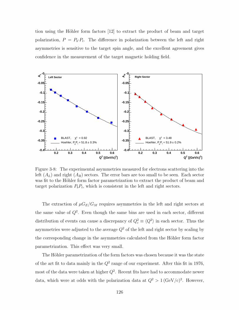
tion using the Hohler form factors [12] to extract the product of beam and target

polarization, P = Pb·Pt. The difference in polarization between the left and right

asymmetries is sensitive to the target spin angle, and the excellent agreement gives

confidence in the measurement of the target magnetic holding field.

]2 [(GeV/c)2Q

0.2 0.3 0.4 0.5 0.6

LA

-0.4

-0.35

-0.3

-0.25

-0.2

-0.15

-0.1

-0.05

-0

= 0.922χBLAST,

0.3%± = 51.8 tPb

Hoehler, P

Left Sector

]2 [(GeV/c)2Q

0.2 0.3 0.4 0.5 0.6

RA

-0.4

-0.35

-0.3

-0.25

-0.2

-0.15

-0.1

-0.05

-0

= 3.482χBLAST,

0.2%± = 51.9 tPb

Hoehler, P

Right Sector

Figure 3-8: The experimental asymmetries measured for electrons scattering into theleft (AL) and right (AR) sectors. The error bars are too small to be seen. Each sectorwas fit to the Hohler form factor parametrization to extract the product of beam andtarget polarization PbPt, which is consistent in the left and right sectors.

The extraction of µGE/GM requires asymmetries in the left and right sectors at

the same value of Q2. Even though the same bins are used in each sector, different

distribution of events can cause a discrepancy of Q2c ≡ 〈Q2〉 in each sector. Thus the

asymmetries were adjusted to the average Q2 of the left and right sector by scaling by

the corresponding change in the asymmetries calculated from the Hohler form factor

parametrization. This effect was very small.

The Hohler parametrization of the form factors was chosen because it was the state

of the art fit to data mainly in the Q2 range of our experiment. After this fit in 1976,

most of the data were taken at higher Q2. Recent fits have had to accommodate newer

data, which were at odds with the polarization data at Q2 > 1 (GeV/c)2. However,

126

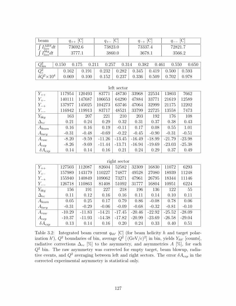
beam q++ [C] q+− [C] q−+ [C] q−− [C]∫IABSlive dt 73692.6 73823.0 73337.4 72821.7∫

Ibkglivedt 3777.1 3860.0 3678.1 3566.2

Q2bin 0.150 0.175 0.211 0.257 0.314 0.382 0.461 0.550 0.650

Q2c 0.162 0.191 0.232 0.282 0.345 0.419 0.500 0.593

δQ2×104 0.069 0.100 0.152 0.237 0.336 0.509 0.702 0.978

left sectorY++ 117954 120493 83771 48730 33968 22534 13803 7662Y+− 140111 147687 106653 64290 47884 33771 21619 12589Y−+ 137977 145025 104273 63746 47064 32999 21175 12202Y−− 116942 119913 83717 48521 33799 22725 13558 7473Ybkg 163 207 221 210 203 192 176 108∆rc 0.21 0.24 0.29 0.32 0.31 0.37 0.38 0.43Abeam 0.16 0.16 0.19 -0.11 0.17 0.08 0.55 1.01Atarg -0.31 -0.48 -0.69 -0.22 -0.45 -0.90 -0.31 -0.51Araw -8.20 -9.59 -11.26 -13.45 -16.49 -18.99 -21.79 -23.98Aexp -8.26 -9.69 -11.44 -13.71 -16.94 -19.69 -23.03 -25.38δAexp 0.14 0.14 0.16 0.21 0.24 0.29 0.37 0.49

right sectorY++ 127503 112087 82604 52582 32309 16830 11072 6293Y+− 157989 143179 110227 74877 49528 27080 18939 11248Y−+ 155940 140849 109062 73271 47961 26795 18344 11146Y−− 126718 110863 81408 51092 31777 16804 10951 6224Ybkg 156 191 227 218 196 136 122 55∆rc 0.11 0.12 0.16 0.16 0.11 0.14 0.10 0.11Abeam 0.05 0.25 0.17 0.79 0.86 -0.08 0.78 0.06Atarg -0.31 -0.29 -0.06 -0.09 -0.68 -0.32 -0.81 -0.10Araw -10.29 -11.83 -14.21 -17.45 -20.46 -22.92 -25.52 -28.09Aexp -10.37 -11.93 -14.38 -17.82 -20.99 -23.69 -26.58 -29.04δAexp 0.13 0.14 0.16 0.20 0.24 0.33 0.40 0.51

Table 3.2: Integrated beam current qhh′ [C] (for beam helicity h and target polar-ization h′), Q2 boundaries of bin, average Q2 [ (GeV/c)2] in bin, yields Yhh′ [counts],radiative corrections ∆rc [%] to the asymmetry, and asymmetries A [%], for eachQ2 bin. The raw asymmetry was corrected for empty target, beam blowup, radia-tive events, and Q2 averaging between left and right sectors. The error δAexp in thecorrected experimental asymmetry is statistical only.

127

these form factors are only used as systematic checks of the data and to bin center

Q2, so their impact on the analysis is minimal.

3.2.2 Background Correction

There is a small contribution to the raw yields from quasi-elastic scattering from the

aluminum target cell wall, and shower events from the collimator upstream of the

target. However, almost all events from the collimator are reconstructed upstream

of the vertex cut, and can be differentiated by their low momentum. In addition,

the collimator reduces the background from the cell wall to less than 0.5% in all

Q2 bins with a 2.5σ cut on the elastic peak in the invariant mass (W ) spectrum.

Both of these processes are helicity independent and can be corrected as a dilution to

the asymmetry. The only background from the hydrogen target is radiative events,

discussed below. The elastic peak is separated from the pion production threshold

by 5 times the resolution of W , so the contribution to the asymmetry from inelastic

scattering is insignificant.

The background was measured under the same conditions as the hydrogen data,

but with the ABS gas flow turned off, and scaled by the ratio of integrated charge

between the two datasets. However, gas in the target can affect the beam profile,

possibly increasing the background rates at the same beam current [153]. This beam

blowup effect was quantified in BLAST [133] through the (e, e′n) quasi-elastic channel.

Since there are no neutrons in the hydrogen target, this channel measures strictly the

background, even in the presence of the hydrogen target. The ratio of (e, e′n) yields

from hydrogen Y nH versus empty target Y n

bkg was fbeam ≡ Y nH/Y n

bkg ≈ 1.05. With

the low backgrounds of BLAST, the beam blowup effect was insignificant. The raw

asymmetry was corrected by

A =Araw

1− fbeamYbkg/YH

, (3.7)

where YH is the unpolarized elastic yield from the ABS hydrogen target and Ybkg

is the same from an empty target. The background distribution is shown with the

128

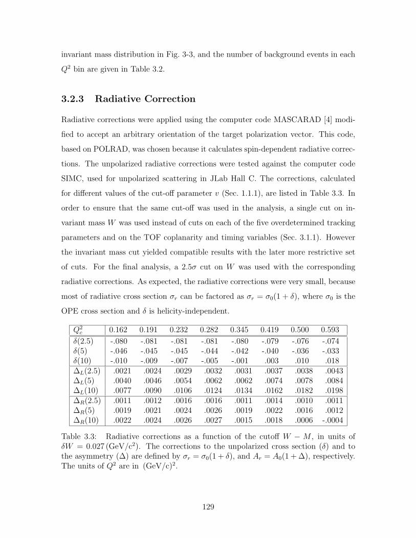
invariant mass distribution in Fig. 3-3, and the number of background events in each

Q2 bin are given in Table 3.2.

3.2.3 Radiative Correction

Radiative corrections were applied using the computer code MASCARAD [4] modi-

fied to accept an arbitrary orientation of the target polarization vector. This code,

based on POLRAD, was chosen because it calculates spin-dependent radiative correc-

tions. The unpolarized radiative corrections were tested against the computer code

SIMC, used for unpolarized scattering in JLab Hall C. The corrections, calculated

for different values of the cut-off parameter v (Sec. 1.1.1), are listed in Table 3.3. In

order to ensure that the same cut-off was used in the analysis, a single cut on in-

variant mass W was used instead of cuts on each of the five overdetermined tracking

parameters and on the TOF coplanarity and timing variables (Sec. 3.1.1). However

the invariant mass cut yielded compatible results with the later more restrictive set

of cuts. For the final analysis, a 2.5σ cut on W was used with the corresponding

radiative corrections. As expected, the radiative corrections were very small, because

most of radiative cross section σr can be factored as σr = σ0(1 + δ), where σ0 is the

OPE cross section and δ is helicity-independent.

Q2c 0.162 0.191 0.232 0.282 0.345 0.419 0.500 0.593

δ(2.5) -.080 -.081 -.081 -.081 -.080 -.079 -.076 -.074δ(5) -.046 -.045 -.045 -.044 -.042 -.040 -.036 -.033δ(10) -.010 -.009 -.007 -.005 -.001 .003 .010 .018∆L(2.5) .0021 .0024 .0029 .0032 .0031 .0037 .0038 .0043∆L(5) .0040 .0046 .0054 .0062 .0062 .0074 .0078 .0084∆L(10) .0077 .0090 .0106 .0124 .0134 .0162 .0182 .0198∆R(2.5) .0011 .0012 .0016 .0016 .0011 .0014 .0010 .0011∆R(5) .0019 .0021 .0024 .0026 .0019 .0022 .0016 .0012∆R(10) .0022 .0024 .0026 .0027 .0015 .0018 .0006 -.0004

Table 3.3: Radiative corrections as a function of the cutoff W − M , in units ofδW = 0.027 (GeV/c2). The corrections to the unpolarized cross section (δ) and tothe asymmetry (∆) are defined by σr = σ0(1 + δ), and Ar = A0(1 + ∆), respectively.The units of Q2 are in (GeV/c)2.

129

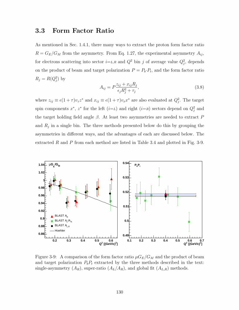
3.3 Form Factor Ratio

As mentioned in Sec. 1.4.1, there many ways to extract the proton form factor ratio

R = GE/GM from the asymmetry. From Eq. 1.27, the experimental asymmetry Aij,

for electrons scattering into sector i=L,R and Q2 bin j of average value Q2j , depends

on the product of beam and target polarization P = Pb·Pt, and the form factor ratio

Rj = R(Q2j) by

Aij = Pzij + xijRj

εjR2j + τj

, (3.8)

where zij ≡ ε(1 + τ)vzz∗ and xij ≡ ε(1 + τ)vxx

∗ are also evaluated at Q2j . The target

spin components x∗, z∗ for the left (i=L) and right (i=R) sectors depend on Q2j and

the target holding field angle β. At least two asymmetries are needed to extract P

and Rj in a single bin. The three methods presented below do this by grouping the

asymmetries in different ways, and the advantages of each are discussed below. The

extracted R and P from each method are listed in Table 3.4 and plotted in Fig. 3-9.

]2 [(GeV/c)2Q0.2 0.3 0.4 0.5 0.6

0.86

0.88

0.9

0.92

0.94

0.96

0.98

1

1.02

1.04

RBLAST A

R/ALBLAST A

L,RBLAST A

Hoehler

M/GE

Gµ

]2 [(GeV/c)2Q0.1 0.2 0.3 0.4 0.5 0.6 0.7

0.49

0.5

0.51

0.52

0.53

0.54tPbP

Figure 3-9: A comparison of the form factor ratio µGE/GM and the product of beamand target polarization PbPt extracted by the three methods described in the text:single-asymmetry (AR), super-ratio (AL/AR), and global fit (AL,R) methods.

130

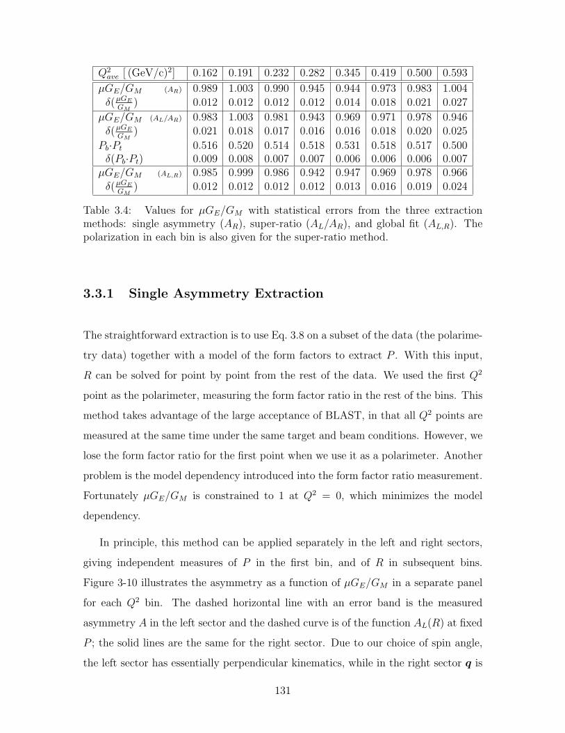
Q2ave [ (GeV/c)2] 0.162 0.191 0.232 0.282 0.345 0.419 0.500 0.593

µGE/GM (AR) 0.989 1.003 0.990 0.945 0.944 0.973 0.983 1.004

δ(µGE

GM) 0.012 0.012 0.012 0.012 0.014 0.018 0.021 0.027

µGE/GM (AL/AR) 0.983 1.003 0.981 0.943 0.969 0.971 0.978 0.946

δ(µGE

GM) 0.021 0.018 0.017 0.016 0.016 0.018 0.020 0.025

Pb·Pt 0.516 0.520 0.514 0.518 0.531 0.518 0.517 0.500δ(Pb·Pt) 0.009 0.008 0.007 0.007 0.006 0.006 0.006 0.007

µGE/GM (AL,R) 0.985 0.999 0.986 0.942 0.947 0.969 0.978 0.966

δ(µGE

GM) 0.012 0.012 0.012 0.012 0.013 0.016 0.019 0.024

Table 3.4: Values for µGE/GM with statistical errors from the three extractionmethods: single asymmetry (AR), super-ratio (AL/AR), and global fit (AL,R). Thepolarization in each bin is also given for the super-ratio method.

3.3.1 Single Asymmetry Extraction

The straightforward extraction is to use Eq. 3.8 on a subset of the data (the polarime-

try data) together with a model of the form factors to extract P . With this input,

R can be solved for point by point from the rest of the data. We used the first Q2

point as the polarimeter, measuring the form factor ratio in the rest of the bins. This

method takes advantage of the large acceptance of BLAST, in that all Q2 points are

measured at the same time under the same target and beam conditions. However, we

lose the form factor ratio for the first point when we use it as a polarimeter. Another

problem is the model dependency introduced into the form factor ratio measurement.

Fortunately µGE/GM is constrained to 1 at Q2 = 0, which minimizes the model

dependency.

In principle, this method can be applied separately in the left and right sectors,

giving independent measures of P in the first bin, and of R in subsequent bins.

Figure 3-10 illustrates the asymmetry as a function of µGE/GM in a separate panel

for each Q2 bin. The dashed horizontal line with an error band is the measured

asymmetry A in the left sector and the dashed curve is of the function AL(R) at fixed

P ; the solid lines are the same for the right sector. Due to our choice of spin angle,

the left sector has essentially perpendicular kinematics, while in the right sector q is

131

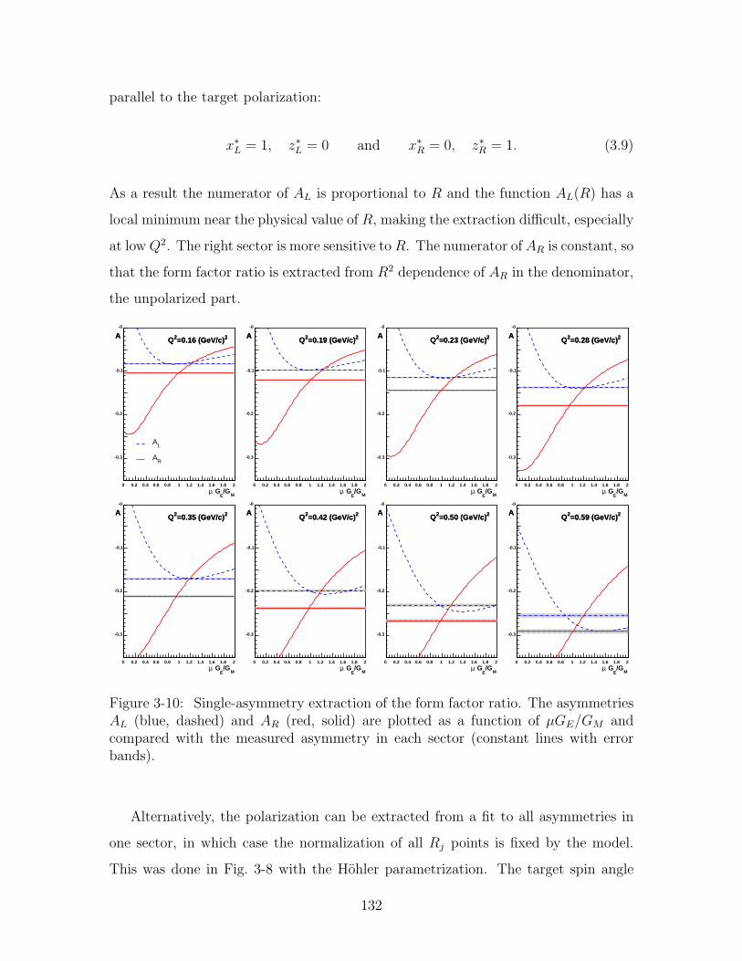
parallel to the target polarization:

x∗L = 1, z∗L = 0 and x∗R = 0, z∗R = 1. (3.9)

As a result the numerator of AL is proportional to R and the function AL(R) has a

local minimum near the physical value of R, making the extraction difficult, especially

at low Q2. The right sector is more sensitive to R. The numerator of AR is constant, so

that the form factor ratio is extracted from R2 dependence of AR in the denominator,

the unpolarized part.

M/G

E Gµ

0 0.2 0.4 0.6 0.8 1 1.2 1.4 1.6 1.8 2

-0.3

-0.2

-0.1

-0

2=0.16 (GeV/c)2QA 2=0.16 (GeV/c)2QA

L A

R A

M/G

E Gµ

0 0.2 0.4 0.6 0.8 1 1.2 1.4 1.6 1.8 2

-0.3

-0.2

-0.1

-0

2=0.19 (GeV/c)2QA 2=0.19 (GeV/c)2QA

M/G

E Gµ

0 0.2 0.4 0.6 0.8 1 1.2 1.4 1.6 1.8 2

-0.3

-0.2

-0.1

-0

2=0.23 (GeV/c)2QA 2=0.23 (GeV/c)2QA

M/G

E Gµ

0 0.2 0.4 0.6 0.8 1 1.2 1.4 1.6 1.8 2

-0.3

-0.2

-0.1

-0

2=0.28 (GeV/c)2QA 2=0.28 (GeV/c)2QA

M/G

E Gµ

0 0.2 0.4 0.6 0.8 1 1.2 1.4 1.6 1.8 2

-0.3

-0.2

-0.1

-0

2=0.35 (GeV/c)2QA 2=0.35 (GeV/c)2QA

M/G

E Gµ

0 0.2 0.4 0.6 0.8 1 1.2 1.4 1.6 1.8 2

-0.3

-0.2

-0.1

-0

2=0.42 (GeV/c)2QA 2=0.42 (GeV/c)2QA

M/G

E Gµ

0 0.2 0.4 0.6 0.8 1 1.2 1.4 1.6 1.8 2

-0.3

-0.2

-0.1

-0

2=0.50 (GeV/c)2QA 2=0.50 (GeV/c)2QA

M/G

E Gµ

0 0.2 0.4 0.6 0.8 1 1.2 1.4 1.6 1.8 2

-0.3

-0.2

-0.1

-0

2=0.59 (GeV/c)2QA 2=0.59 (GeV/c)2QA

Figure 3-10: Single-asymmetry extraction of the form factor ratio. The asymmetriesAL (blue, dashed) and AR (red, solid) are plotted as a function of µGE/GM andcompared with the measured asymmetry in each sector (constant lines with errorbands).

Alternatively, the polarization can be extracted from a fit to all asymmetries in

one sector, in which case the normalization of all Rj points is fixed by the model.

This was done in Fig. 3-8 with the Hohler parametrization. The target spin angle

132

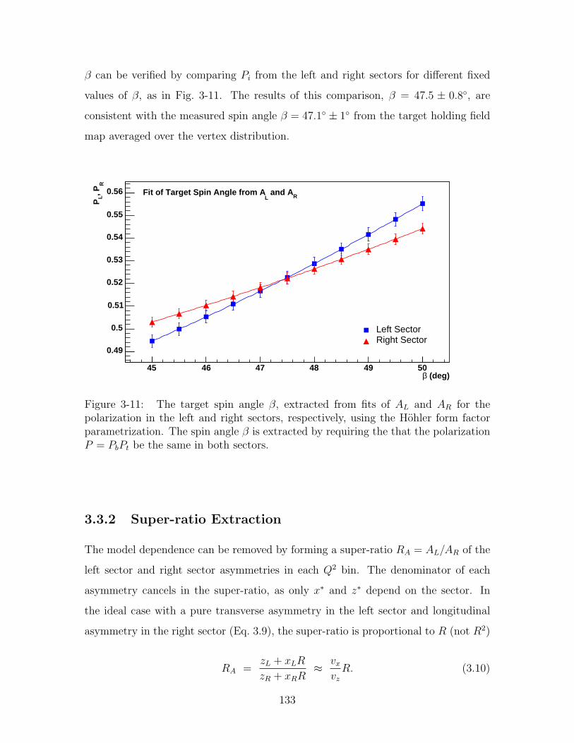
β can be verified by comparing Pi from the left and right sectors for different fixed

values of β, as in Fig. 3-11. The results of this comparison, β = 47.5 ± 0.8, are

consistent with the measured spin angle β = 47.1 ± 1 from the target holding field

map averaged over the vertex distribution.

(deg)β45 46 47 48 49 50

R, P L

P

0.49

0.5

0.51

0.52

0.53

0.54

0.55

0.56

Left SectorRight Sector

R and AL

Fit of Target Spin Angle from A

Figure 3-11: The target spin angle β, extracted from fits of AL and AR for thepolarization in the left and right sectors, respectively, using the Hohler form factorparametrization. The spin angle β is extracted by requiring the that the polarizationP = PbPt be the same in both sectors.

3.3.2 Super-ratio Extraction

The model dependence can be removed by forming a super-ratio RA = AL/AR of the

left sector and right sector asymmetries in each Q2 bin. The denominator of each

asymmetry cancels in the super-ratio, as only x∗ and z∗ depend on the sector. In

the ideal case with a pure transverse asymmetry in the left sector and longitudinal

asymmetry in the right sector (Eq. 3.9), the super-ratio is proportional to R (not R2)

RA =zL + xLR

zR + xRR≈ vx

vz

R. (3.10)

133

R can be substituted back into Eq. 3.8 for either the left or right sector to extract

the polarization.

Instead of directly forming the super-ratio as above, both R and P can be solved

from AL, AR by transforming Eq. 3.8 for AL and AR into the linear equation(−x∗L AL

−x∗R AR

)(vxRvz

εR2+τε(1+τ)vzP

)=

(z∗L

z∗R

)(3.11)

with the solution

R = −vz

vx

· z∗LAR − z∗RAL

x∗LAR − x∗RAL

(3.12)

and

P =εR2 + τ

ε(1+τ)vz

· x∗LAR − x∗RAL

x∗Lz∗R − x∗Rz∗L. (3.13)

Another advantage of the super-ratio method beside model independency is that

an independent polarization Pj can be extracted in each Q2 bin. This is an important

check on systematic errors. Also, if an unanticipated dilution is the same in both

sectors and depends only on Q2 (not the spin angle), then it can be absorbed into

Pj. In this case the extracted form factor ratio will still be accurate. However, from

Eq. 3.13 it is apparent that one cannot compare polarizations from the left and right

sector using this method. In Fig. 3-9, the polarization in all bins except possibly the

last are consistent with each other.

3.3.3 Global Fit Extraction

The third extraction combines the strengths of the two previous methods by fitting

both the left and right sector asymmetries for P . Instead of relying on a model

for the form factors Rj in the fit, they are included as free parameters, extracted

simultaneously with P . This method takes advantage of both the symmetric left and

right sectors and the large acceptance of BLAST.

The fit makes optimal use of the asymmetry information in extracting P and Rj,

and has the lowest statistical uncertainty in Rj of the three methods. Compared

to the single asymmetry method, the fits of P in each sector are combined into a

134

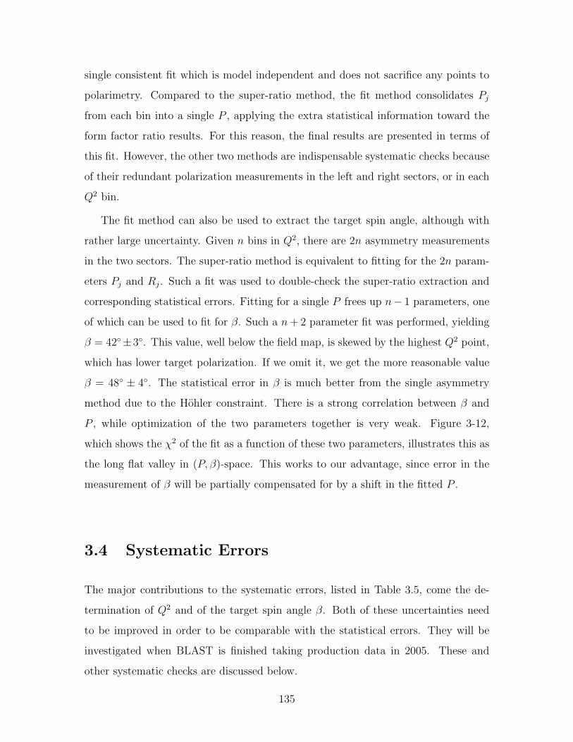
single consistent fit which is model independent and does not sacrifice any points to

polarimetry. Compared to the super-ratio method, the fit method consolidates Pj

from each bin into a single P , applying the extra statistical information toward the

form factor ratio results. For this reason, the final results are presented in terms of

this fit. However, the other two methods are indispensable systematic checks because

of their redundant polarization measurements in the left and right sectors, or in each

Q2 bin.

The fit method can also be used to extract the target spin angle, although with

rather large uncertainty. Given n bins in Q2, there are 2n asymmetry measurements

in the two sectors. The super-ratio method is equivalent to fitting for the 2n param-

eters Pj and Rj. Such a fit was used to double-check the super-ratio extraction and

corresponding statistical errors. Fitting for a single P frees up n− 1 parameters, one

of which can be used to fit for β. Such a n + 2 parameter fit was performed, yielding

β = 42±3. This value, well below the field map, is skewed by the highest Q2 point,

which has lower target polarization. If we omit it, we get the more reasonable value

β = 48 ± 4. The statistical error in β is much better from the single asymmetry

method due to the Hohler constraint. There is a strong correlation between β and

P , while optimization of the two parameters together is very weak. Figure 3-12,

which shows the χ2 of the fit as a function of these two parameters, illustrates this as

the long flat valley in (P, β)-space. This works to our advantage, since error in the

measurement of β will be partially compensated for by a shift in the fitted P .

3.4 Systematic Errors

The major contributions to the systematic errors, listed in Table 3.5, come the de-

termination of Q2 and of the target spin angle β. Both of these uncertainties need

to be improved in order to be comparable with the statistical errors. They will be

investigated when BLAST is finished taking production data in 2005. These and

other systematic checks are discussed below.

135

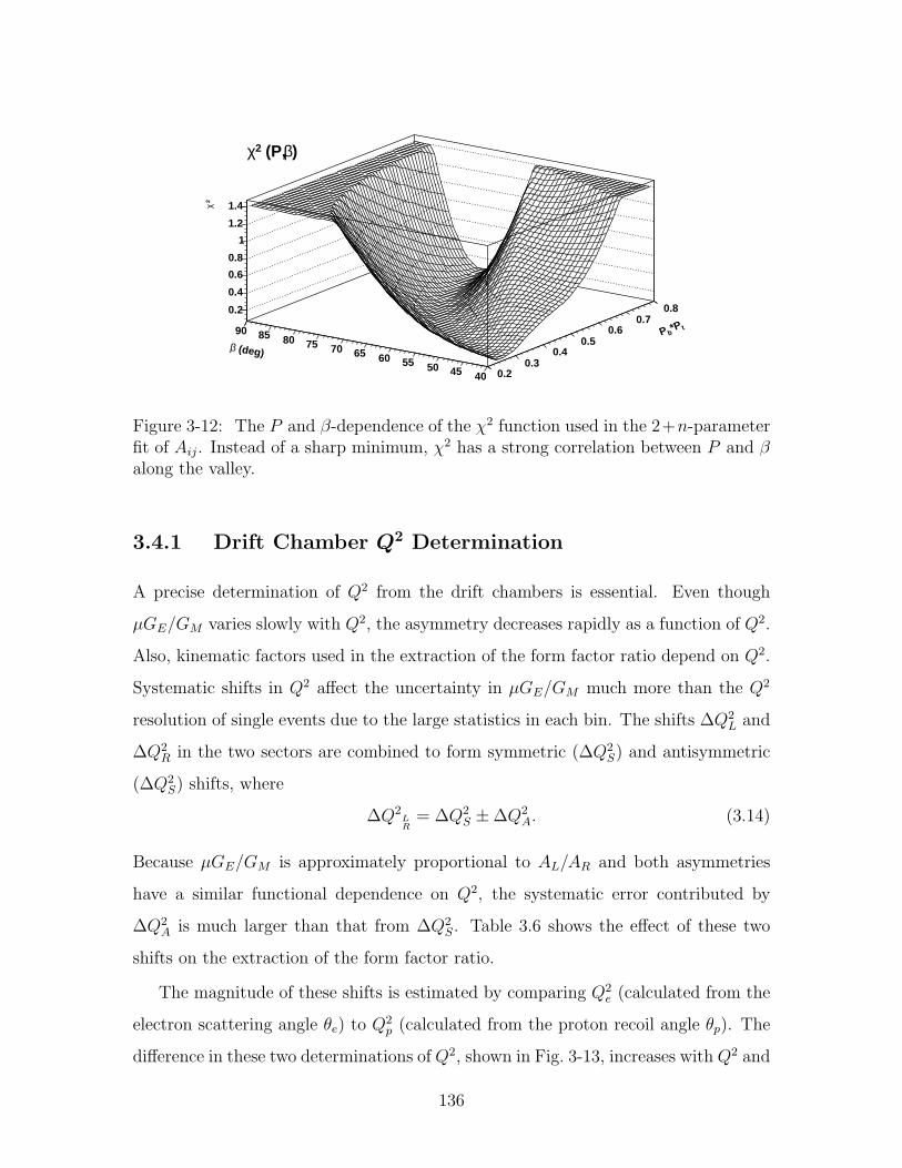
t*PbP

0.20.3

0.40.5

0.60.7

0.8

(deg)β

4045505560657075808590

2χ

0.2

0.4

0.6

0.8

1

1.2

1.4

)β (P,2χ

Figure 3-12: The P and β-dependence of the χ2 function used in the 2+n-parameterfit of Aij. Instead of a sharp minimum, χ2 has a strong correlation between P and βalong the valley.

3.4.1 Drift Chamber Q2 Determination

A precise determination of Q2 from the drift chambers is essential. Even though

µGE/GM varies slowly with Q2, the asymmetry decreases rapidly as a function of Q2.

Also, kinematic factors used in the extraction of the form factor ratio depend on Q2.

Systematic shifts in Q2 affect the uncertainty in µGE/GM much more than the Q2

resolution of single events due to the large statistics in each bin. The shifts ∆Q2L and

∆Q2R in the two sectors are combined to form symmetric (∆Q2

S) and antisymmetric

(∆Q2S) shifts, where

∆Q2LR

= ∆Q2S ±∆Q2

A. (3.14)

Because µGE/GM is approximately proportional to AL/AR and both asymmetries

have a similar functional dependence on Q2, the systematic error contributed by

∆Q2A is much larger than that from ∆Q2

S. Table 3.6 shows the effect of these two

shifts on the extraction of the form factor ratio.

The magnitude of these shifts is estimated by comparing Q2e (calculated from the

electron scattering angle θe) to Q2p (calculated from the proton recoil angle θp). The

difference in these two determinations of Q2, shown in Fig. 3-13, increases with Q2 and

136

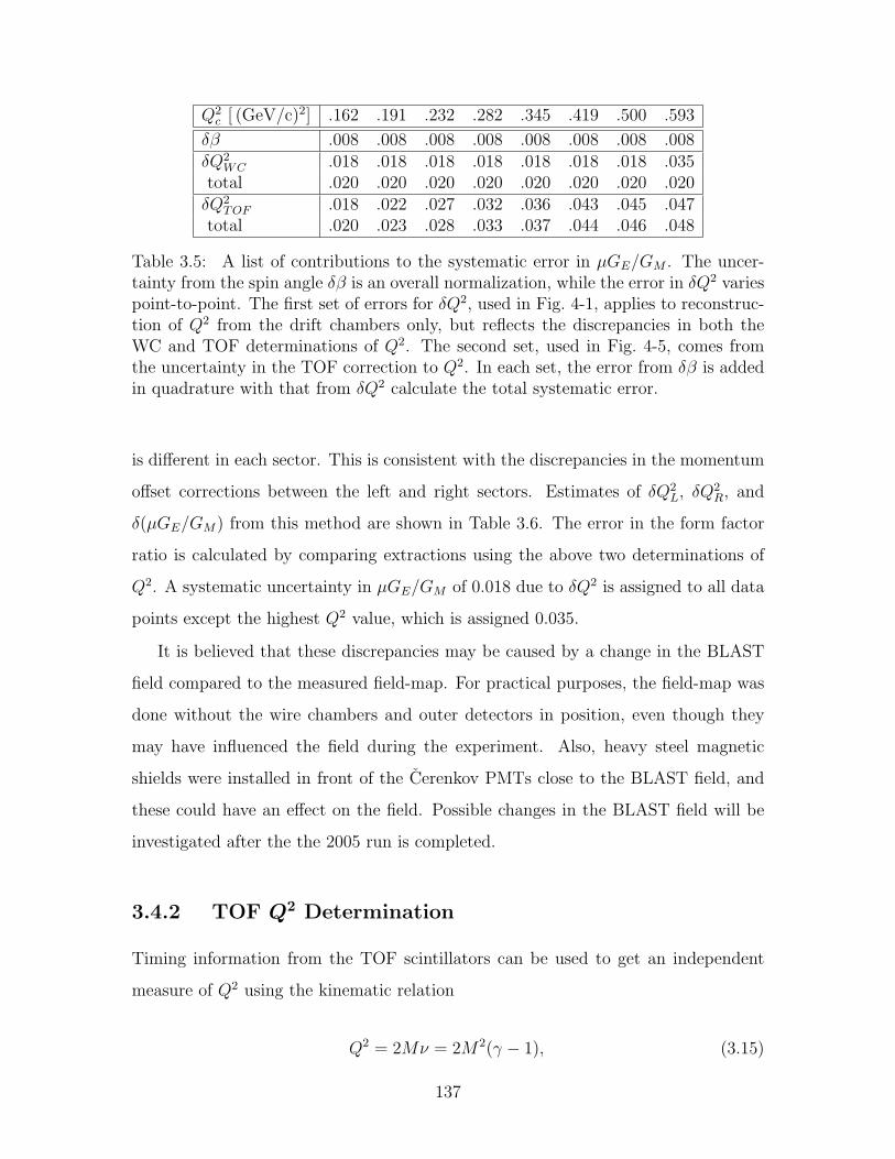
Q2c [ (GeV/c)2] .162 .191 .232 .282 .345 .419 .500 .593

δβ .008 .008 .008 .008 .008 .008 .008 .008δQ2

WC .018 .018 .018 .018 .018 .018 .018 .035total .020 .020 .020 .020 .020 .020 .020 .020δQ2

TOF .018 .022 .027 .032 .036 .043 .045 .047total .020 .023 .028 .033 .037 .044 .046 .048

Table 3.5: A list of contributions to the systematic error in µGE/GM . The uncer-tainty from the spin angle δβ is an overall normalization, while the error in δQ2 variespoint-to-point. The first set of errors for δQ2, used in Fig. 4-1, applies to reconstruc-tion of Q2 from the drift chambers only, but reflects the discrepancies in both theWC and TOF determinations of Q2. The second set, used in Fig. 4-5, comes fromthe uncertainty in the TOF correction to Q2. In each set, the error from δβ is addedin quadrature with that from δQ2 calculate the total systematic error.

is different in each sector. This is consistent with the discrepancies in the momentum

offset corrections between the left and right sectors. Estimates of δQ2L, δQ2

R, and

δ(µGE/GM) from this method are shown in Table 3.6. The error in the form factor

ratio is calculated by comparing extractions using the above two determinations of

Q2. A systematic uncertainty in µGE/GM of 0.018 due to δQ2 is assigned to all data

points except the highest Q2 value, which is assigned 0.035.

It is believed that these discrepancies may be caused by a change in the BLAST

field compared to the measured field-map. For practical purposes, the field-map was

done without the wire chambers and outer detectors in position, even though they

may have influenced the field during the experiment. Also, heavy steel magnetic

shields were installed in front of the Cerenkov PMTs close to the BLAST field, and

these could have an effect on the field. Possible changes in the BLAST field will be

investigated after the the 2005 run is completed.

3.4.2 TOF Q2 Determination

Timing information from the TOF scintillators can be used to get an independent

measure of Q2 using the kinematic relation

Q2 = 2Mν = 2M2(γ − 1), (3.15)

137

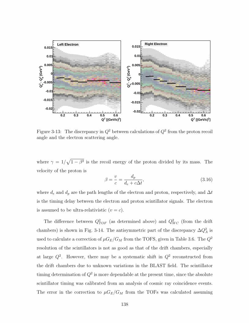
Left Electron

]2 [(GeV/c)2Q0.2 0.3 0.4 0.5 0.6

)2 (

GeV

p2 -

Qe2

Q

-0.02

-0.015

-0.01

-0.005

0

0.005

0.01

0.015Right Electron

]2 [(GeV/c)2Q0.2 0.3 0.4 0.5 0.6

)2 (

GeV

p2 -

Qe2

Q

-0.02

-0.015

-0.01

-0.005

0

0.005

0.01

0.015

Figure 3-13: The discrepancy in Q2 between calculations of Q2 from the proton recoilangle and the electron scattering angle.

where γ = 1/√

1− β2 is the recoil energy of the proton divided by its mass. The

velocity of the proton is

β =v

c=

dp

de + c∆t, (3.16)

where de and dp are the path lengths of the electron and proton, respectively, and ∆t

is the timing delay between the electron and proton scintillator signals. The electron

is assumed to be ultra-relativistic (v = c).

The difference between Q2TOF (as determined above) and Q2

WC (from the drift

chambers) is shown in Fig. 3-14. The antisymmetric part of the discrepancy ∆Q2A is

used to calculate a correction of µGE/GM from the TOFS, given in Table 3.6. The Q2

resolution of the scintillators is not as good as that of the drift chambers, especially

at large Q2. However, there may be a systematic shift in Q2 reconstructed from

the drift chambers due to unknown variations in the BLAST field. The scintillator

timing determination of Q2 is more dependable at the present time, since the absolute

scintillator timing was calibrated from an analysis of cosmic ray coincidence events.

The error in the correction to µGE/GM from the TOFs was calculated assuming

138

]2 [(GeV/c)WC2Q

0.2 0.3 0.4 0.5 0.6

)2 (

GeV

WC

2-

QT

OF

2

Q

-0.06

-0.04

-0.02

0

0.02

0.04

0.06 left electron

]2 [(GeV/c)WC2Q

0.2 0.3 0.4 0.5 0.6

)2 (

GeV

WC

2-

QT

OF

2

Q

-0.06

-0.04

-0.02

0

0.02

0.04

0.06 right electron

Figure 3-14: Comparison of Q2 from the TOF scintillators and the drift chambers.The two vertical bands are caused by the omission of TOF 9 in the left and rightsector.

150 ps systematic errors in timing. Work is being done to push this error down to 1

channel (50 ps) with a more thorough calibration of the timing offsets with cosmic

rays.

There are plans to investigate the difference between TOF and drift chamber

reconstruction after the 2005 run. After the cause of the discrepancies is understood

and corrected, the systematics will be further reduced by performing a kinematic

fit for Q2 of each event with combined data from both the drift chamber and TOF

scintillator hits.

3.4.3 Target Spin Angle

Precise knowledge of the target holding field angle is also important. After the hy-

drogen production run, a careful map of the holding field was done using a 3-D Hall

probe and a special jig to align the probe with respect to the scattering chamber.

The alignment of the Hall probe was measured by inserting it in a uniform dipole

field. However, geometric restrictions prevented a precise measurement of one of the

orientation angles of the Hall probe, which was unfortunately in the same direction as

139

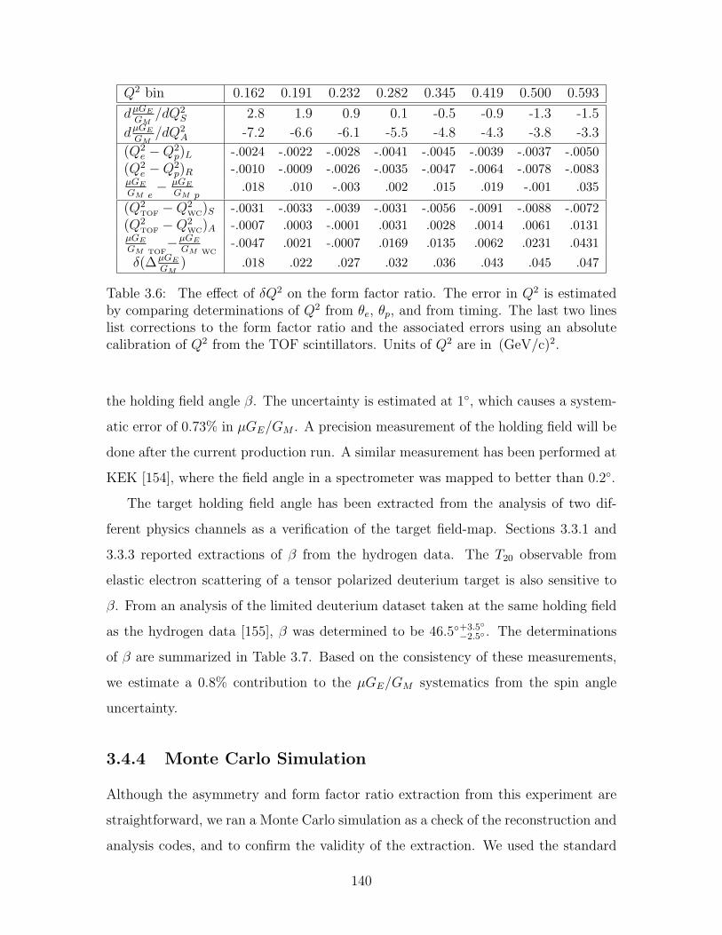
Q2 bin 0.162 0.191 0.232 0.282 0.345 0.419 0.500 0.593

dµGE

GM/dQ2

S 2.8 1.9 0.9 0.1 -0.5 -0.9 -1.3 -1.5

dµGE

GM/dQ2

A -7.2 -6.6 -6.1 -5.5 -4.8 -4.3 -3.8 -3.3

(Q2e −Q2

p)L -.0024 -.0022 -.0028 -.0041 -.0045 -.0039 -.0037 -.0050(Q2

e −Q2p)R -.0010 -.0009 -.0026 -.0035 -.0047 -.0064 -.0078 -.0083

µGE

GM e− µGE

GM p.018 .010 -.003 .002 .015 .019 -.001 .035

(Q2TOF −Q2

WC)S -.0031 -.0033 -.0039 -.0031 -.0056 -.0091 -.0088 -.0072(Q2

TOF −Q2WC)A -.0007 .0003 -.0001 .0031 .0028 .0014 .0061 .0131

µGE

GM TOF−µGE

GM WC-.0047 .0021 -.0007 .0169 .0135 .0062 .0231 .0431

δ(∆µGE

GM) .018 .022 .027 .032 .036 .043 .045 .047

Table 3.6: The effect of δQ2 on the form factor ratio. The error in Q2 is estimatedby comparing determinations of Q2 from θe, θp, and from timing. The last two lineslist corrections to the form factor ratio and the associated errors using an absolutecalibration of Q2 from the TOF scintillators. Units of Q2 are in (GeV/c)2.

the holding field angle β. The uncertainty is estimated at 1, which causes a system-

atic error of 0.73% in µGE/GM . A precision measurement of the holding field will be

done after the current production run. A similar measurement has been performed at

KEK [154], where the field angle in a spectrometer was mapped to better than 0.2.

The target holding field angle has been extracted from the analysis of two dif-

ferent physics channels as a verification of the target field-map. Sections 3.3.1 and

3.3.3 reported extractions of β from the hydrogen data. The T20 observable from

elastic electron scattering of a tensor polarized deuterium target is also sensitive to

β. From an analysis of the limited deuterium dataset taken at the same holding field

as the hydrogen data [155], β was determined to be 46.5+3.5

−2.5 . The determinations

of β are summarized in Table 3.7. Based on the consistency of these measurements,

we estimate a 0.8% contribution to the µGE/GM systematics from the spin angle

uncertainty.

3.4.4 Monte Carlo Simulation

Although the asymmetry and form factor ratio extraction from this experiment are

straightforward, we ran a Monte Carlo simulation as a check of the reconstruction and

analysis codes, and to confirm the validity of the extraction. We used the standard

140

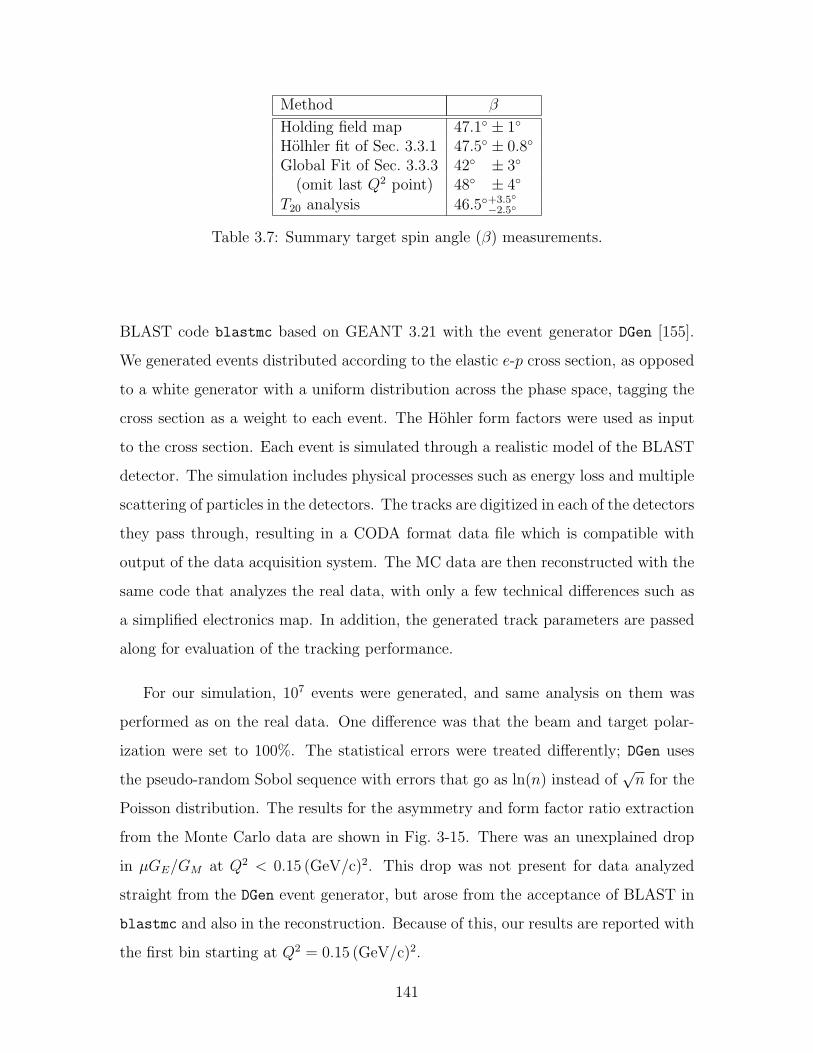
Method β

Holding field map 47.1 ± 1

Holhler fit of Sec. 3.3.1 47.5 ± 0.8

Global Fit of Sec. 3.3.3 42 ± 3

(omit last Q2 point) 48 ± 4

T20 analysis 46.5+3.5

−2.5

Table 3.7: Summary target spin angle (β) measurements.

BLAST code blastmc based on GEANT 3.21 with the event generator DGen [155].

We generated events distributed according to the elastic e-p cross section, as opposed

to a white generator with a uniform distribution across the phase space, tagging the

cross section as a weight to each event. The Hohler form factors were used as input

to the cross section. Each event is simulated through a realistic model of the BLAST

detector. The simulation includes physical processes such as energy loss and multiple

scattering of particles in the detectors. The tracks are digitized in each of the detectors

they pass through, resulting in a CODA format data file which is compatible with

output of the data acquisition system. The MC data are then reconstructed with the

same code that analyzes the real data, with only a few technical differences such as

a simplified electronics map. In addition, the generated track parameters are passed

along for evaluation of the tracking performance.

For our simulation, 107 events were generated, and same analysis on them was

performed as on the real data. One difference was that the beam and target polar-

ization were set to 100%. The statistical errors were treated differently; DGen uses

the pseudo-random Sobol sequence with errors that go as ln(n) instead of√

n for the

Poisson distribution. The results for the asymmetry and form factor ratio extraction

from the Monte Carlo data are shown in Fig. 3-15. There was an unexplained drop

in µGE/GM at Q2 < 0.15 (GeV/c)2. This drop was not present for data analyzed

straight from the DGen event generator, but arose from the acceptance of BLAST in

blastmc and also in the reconstruction. Because of this, our results are reported with

the first bin starting at Q2 = 0.15 (GeV/c)2.

141

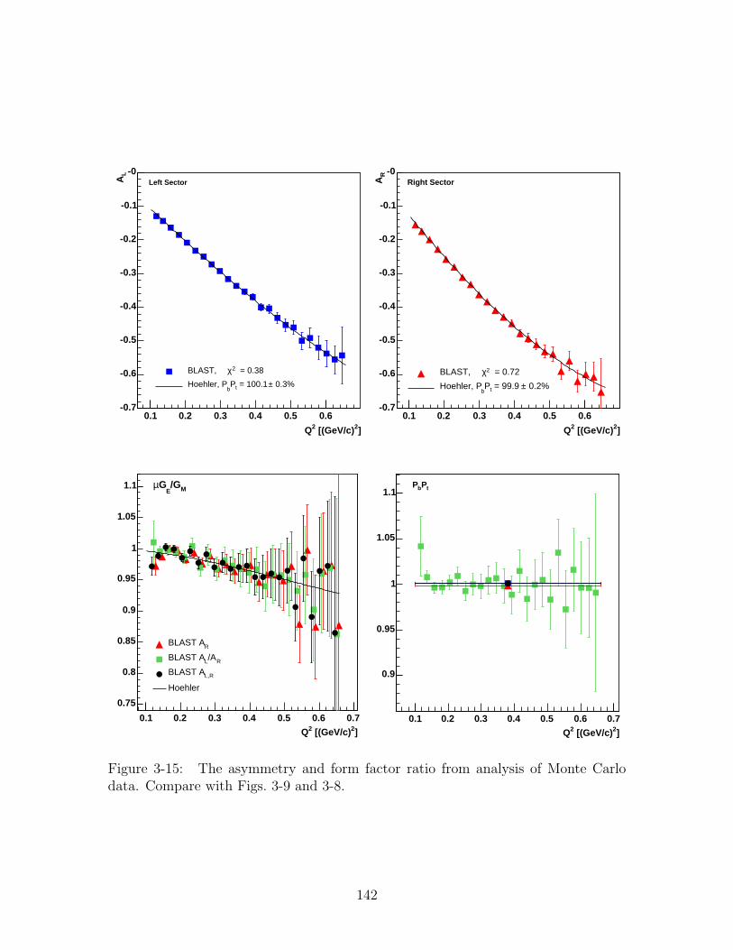
]2 [(GeV/c)2Q

0.1 0.2 0.3 0.4 0.5 0.6

LA

-0.7

-0.6

-0.5

-0.4

-0.3

-0.2

-0.1

-0

= 0.382χBLAST,

0.3%± = 100.1 tPb

Hoehler, P

Left Sector

]2 [(GeV/c)2Q

0.1 0.2 0.3 0.4 0.5 0.6

RA

-0.7

-0.6

-0.5

-0.4

-0.3

-0.2

-0.1

-0

= 0.722χBLAST,

0.2%± = 99.9 tPb

Hoehler, P

Right Sector

]2 [(GeV/c)2Q

0.1 0.2 0.3 0.4 0.5 0.6 0.7

0.75

0.8

0.85

0.9

0.95

1

1.05

1.1

RBLAST A

R/ALBLAST A

L,RBLAST A

Hoehler

M/GE

Gµ

]2 [(GeV/c)2Q

0.1 0.2 0.3 0.4 0.5 0.6 0.7

0.9

0.95

1

1.05

1.1 tPbP

Figure 3-15: The asymmetry and form factor ratio from analysis of Monte Carlodata. Compare with Figs. 3-9 and 3-8.

142

3.4.5 Binning and Cuts

In order to check for binning effects, the analysis was repeated with 24 bins in Q2,

as shown in Fig. 3-16. The discontinuities in the yield of the Q2 = 0.29 (GeV/c)2

bin (Fig. 3-5) were also investigated. As mentioned in Sec. 3.1.4, the whole dataset

was broken into six sets, the first three sets separated by the above discontinuities,

and the last three sets divided equally. The analysis was performed independently on

each data set (Fig. 3-17), and the results of all sets were consistent with each other.

The choice of cuts also had a negligible effect on the asymmetry and extracted

form factor ratio. The analysis was repeated for different combinations of TOF,

Cerenkov , and drift chamber cuts, and the results from each combination were con-

sistent with each other. Cuts on all five redundant tracking parameters from the drift

chambers were compared with a single cut on invariant mass W . There was also little

dependence of the width of cuts. A 2.5σ cut on W was used for the final analysis.

3.4.6 False Asymmetry

There are two independent measures of false asymmetries: the beam helicity asym-

metry averaged over the two target spin states, and vice versa (Eq. 3.6). These

measurements can detect asymmetries in the intensity or polarization between the

two beam or target polarizations or asymmetries in the integrated beam current of

each spin combination. The beam asymmetry Ab is negligible, but there is a small

0.4% target asymmetry At (Fig. 3-18). It is likely due to a difference in the inten-

sity of the two ABS polarization states, as opposed to a true false asymmetry, since

the beam asymmetry is small. There are a number of possible causes: an inefficient

WFT in the ABS, spin-dependence of the target cell temperature due to interference

of readout electronics with the WFT, or random intervals in which the ABS was

temporarily unpolarized. The target asymmetry cancels to first order in the physics

asymmetry by combining all four spin states, and has negligible systematic error.

143

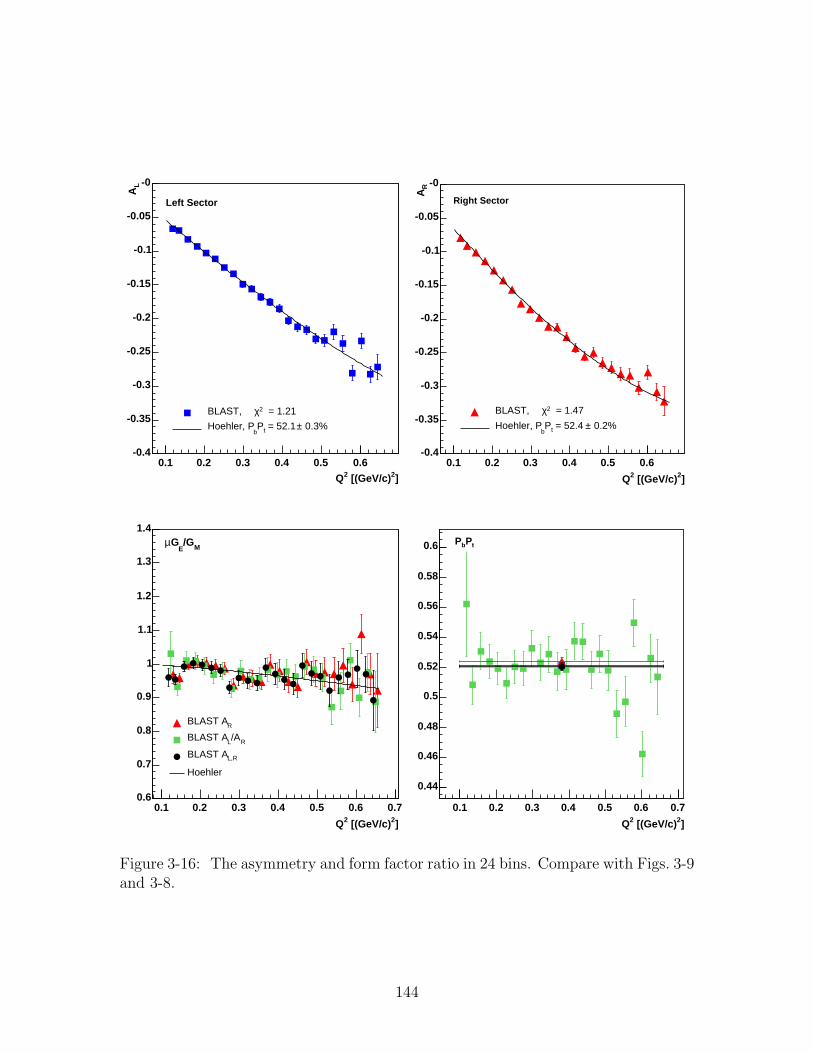
]2 [(GeV/c)2Q

0.1 0.2 0.3 0.4 0.5 0.6

LA

-0.4

-0.35

-0.3

-0.25

-0.2

-0.15

-0.1

-0.05

-0

= 1.212χBLAST,

0.3%± = 52.1 tPb

Hoehler, P

Left Sector

]2 [(GeV/c)2Q

0.1 0.2 0.3 0.4 0.5 0.6

RA

-0.4

-0.35

-0.3

-0.25

-0.2

-0.15

-0.1

-0.05

-0

= 1.472χBLAST,

0.2%± = 52.4 tPb

Hoehler, P

Right Sector

]2 [(GeV/c)2Q

0.1 0.2 0.3 0.4 0.5 0.6 0.70.6

0.7

0.8

0.9

1

1.1

1.2

1.3

1.4

RBLAST A

R/ALBLAST A

L,RBLAST A

Hoehler

M/GE

Gµ

]2 [(GeV/c)2Q

0.1 0.2 0.3 0.4 0.5 0.6 0.7

0.44

0.46

0.48

0.5

0.52

0.54

0.56

0.58

0.6 tPbP

Figure 3-16: The asymmetry and form factor ratio in 24 bins. Compare with Figs. 3-9and 3-8.

144

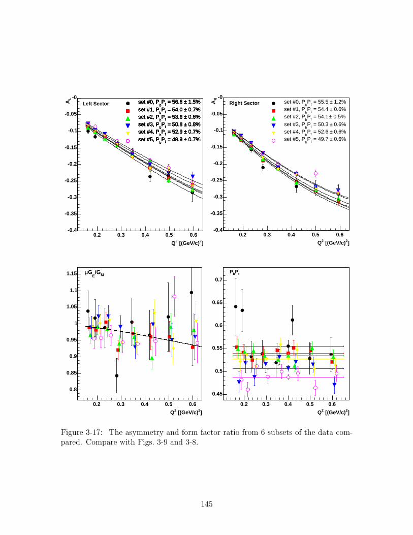
]2 [(GeV/c)2Q

0.2 0.3 0.4 0.5 0.6

LA

-0.4

-0.35

-0.3

-0.25

-0.2

-0.15

-0.1

-0.05

-0 1.5%± = 56.6 tP

bset #0, P

0.7%± = 54.0 tPb

set #1, P 0.6%± = 53.6 tP

bset #2, P

0.8%± = 50.8 tPb

set #3, P 0.7%± = 52.9 tP

bset #4, P

0.7%± = 48.9 tPb

set #5, P

1.5%± = 56.6 tPb

set #0, P

0.7%± = 54.0 tPb

set #1, P 0.6%± = 53.6 tP

bset #2, P

0.8%± = 50.8 tPb

set #3, P 0.7%± = 52.9 tP

bset #4, P

0.7%± = 48.9 tPb

set #5, P

1.5%± = 56.6 tPb

set #0, P

0.7%± = 54.0 tPb

set #1, P 0.6%± = 53.6 tP

bset #2, P

0.8%± = 50.8 tPb

set #3, P 0.7%± = 52.9 tP

bset #4, P

0.7%± = 48.9 tPb

set #5, P

1.5%± = 56.6 tPb

set #0, P

0.7%± = 54.0 tPb

set #1, P 0.6%± = 53.6 tP

bset #2, P

0.8%± = 50.8 tPb

set #3, P 0.7%± = 52.9 tP

bset #4, P

0.7%± = 48.9 tPb

set #5, P

1.5%± = 56.6 tPb

set #0, P

0.7%± = 54.0 tPb

set #1, P 0.6%± = 53.6 tP

bset #2, P

0.8%± = 50.8 tPb

set #3, P 0.7%± = 52.9 tP

bset #4, P

0.7%± = 48.9 tPb

set #5, P

1.5%± = 56.6 tPb

set #0, P

0.7%± = 54.0 tPb

set #1, P 0.6%± = 53.6 tP

bset #2, P

0.8%± = 50.8 tPb

set #3, P 0.7%± = 52.9 tP

bset #4, P

0.7%± = 48.9 tPb

set #5, P

Left Sector

]2 [(GeV/c)2Q

0.2 0.3 0.4 0.5 0.6

RA

-0.4

-0.35

-0.3

-0.25

-0.2

-0.15

-0.1

-0.05

-0 1.2%± = 55.5 tP

bset #0, P

0.6%± = 54.4 tPb

set #1, P 0.5%± = 54.1 tP

bset #2, P

0.6%± = 50.3 tPb

set #3, P 0.6%± = 52.6 tP

bset #4, P

0.6%± = 49.7 tPb

set #5, P

1.2%± = 55.5 tPb

set #0, P 0.6%± = 54.4 tP

bset #1, P

0.5%± = 54.1 tPb

set #2, P

0.6%± = 50.3 tPb

set #3, P 0.6%± = 52.6 tP

bset #4, P

0.6%± = 49.7 tPb

set #5, P

1.2%± = 55.5 tPb

set #0, P 0.6%± = 54.4 tP

bset #1, P

0.5%± = 54.1 tPb

set #2, P

0.6%± = 50.3 tPb

set #3, P 0.6%± = 52.6 tP

bset #4, P

0.6%± = 49.7 tPb

set #5, P

1.2%± = 55.5 tPb

set #0, P 0.6%± = 54.4 tP

bset #1, P

0.5%± = 54.1 tPb

set #2, P

0.6%± = 50.3 tPb

set #3, P 0.6%± = 52.6 tP

bset #4, P

0.6%± = 49.7 tPb

set #5, P

1.2%± = 55.5 tPb

set #0, P 0.6%± = 54.4 tP

bset #1, P

0.5%± = 54.1 tPb

set #2, P

0.6%± = 50.3 tPb

set #3, P 0.6%± = 52.6 tP

bset #4, P

0.6%± = 49.7 tPb

set #5, P

1.2%± = 55.5 tPb

set #0, P 0.6%± = 54.4 tP

bset #1, P

0.5%± = 54.1 tPb

set #2, P

0.6%± = 50.3 tPb

set #3, P 0.6%± = 52.6 tP

bset #4, P

0.6%± = 49.7 tPb

set #5, P

Right Sector

]2 [(GeV/c)2Q

0.2 0.3 0.4 0.5 0.6

0.8

0.85

0.9

0.95

1

1.05

1.1

1.15 M/GE

Gµ

]2 [(GeV/c)2Q

0.2 0.3 0.4 0.5 0.6

0.45

0.5

0.55

0.6

0.65

0.7tPbP

Figure 3-17: The asymmetry and form factor ratio from 6 subsets of the data com-pared. Compare with Figs. 3-9 and 3-8.

145

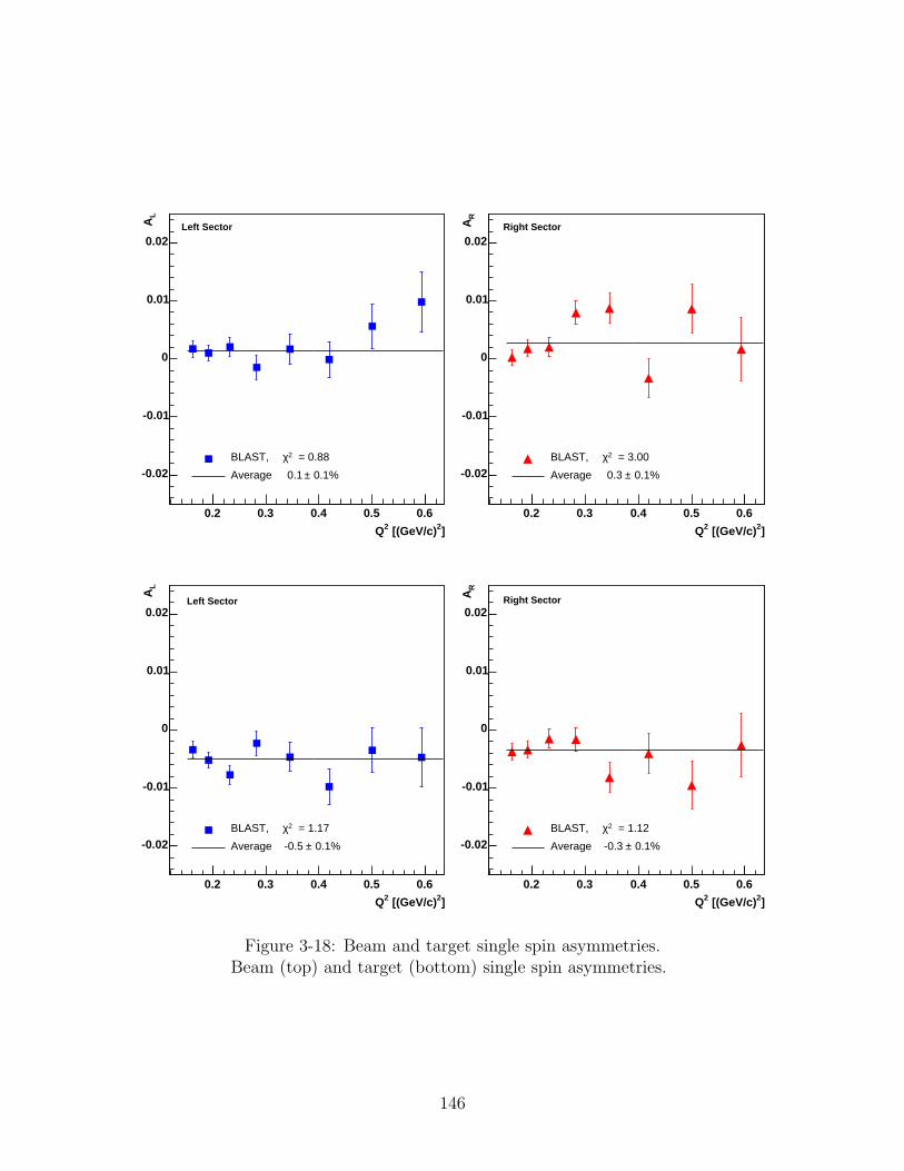
]2 [(GeV/c)2Q

0.2 0.3 0.4 0.5 0.6

LA

-0.02

-0.01

0

0.01

0.02

= 0.882χBLAST,

0.1%±Average 0.1

Left Sector

]2 [(GeV/c)2Q

0.2 0.3 0.4 0.5 0.6

RA

-0.02

-0.01

0

0.01

0.02

= 3.002χBLAST,

0.1%±Average 0.3

Right Sector

]2 [(GeV/c)2Q

0.2 0.3 0.4 0.5 0.6

LA

-0.02

-0.01

0

0.01

0.02

= 1.172χBLAST,

0.1%±Average -0.5

Left Sector

]2 [(GeV/c)2Q

0.2 0.3 0.4 0.5 0.6

RA

-0.02

-0.01

0

0.01

0.02

= 1.122χBLAST,

0.1%±Average -0.3

Right Sector

Figure 3-18: Beam and target single spin asymmetries.Beam (top) and target (bottom) single spin asymmetries.

146

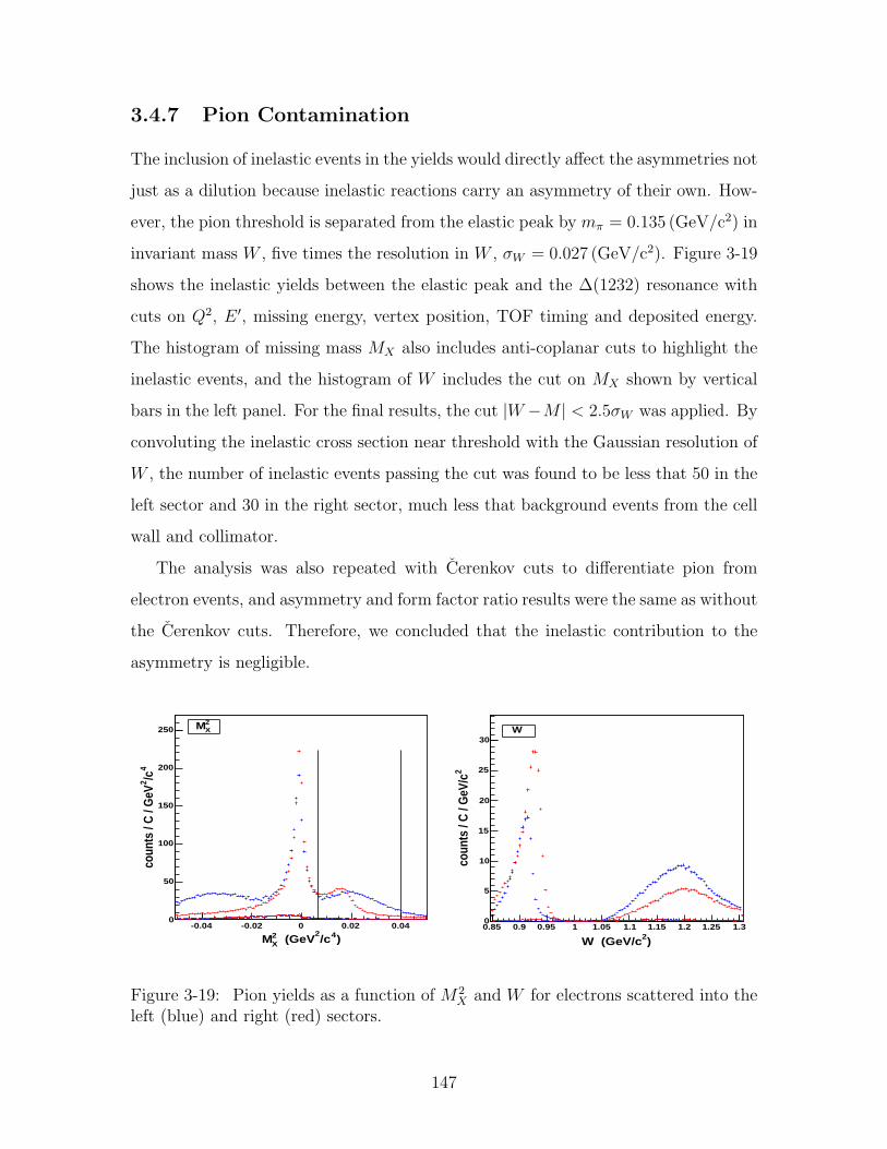
3.4.7 Pion Contamination

The inclusion of inelastic events in the yields would directly affect the asymmetries not

just as a dilution because inelastic reactions carry an asymmetry of their own. How-

ever, the pion threshold is separated from the elastic peak by mπ = 0.135 (GeV/c2) in

invariant mass W , five times the resolution in W , σW = 0.027 (GeV/c2). Figure 3-19

shows the inelastic yields between the elastic peak and the ∆(1232) resonance with

cuts on Q2, E ′, missing energy, vertex position, TOF timing and deposited energy.

The histogram of missing mass MX also includes anti-coplanar cuts to highlight the

inelastic events, and the histogram of W includes the cut on MX shown by vertical

bars in the left panel. For the final results, the cut |W −M | < 2.5σW was applied. By

convoluting the inelastic cross section near threshold with the Gaussian resolution of

W , the number of inelastic events passing the cut was found to be less that 50 in the

left sector and 30 in the right sector, much less that background events from the cell

wall and collimator.

The analysis was also repeated with Cerenkov cuts to differentiate pion from

electron events, and asymmetry and form factor ratio results were the same as without

the Cerenkov cuts. Therefore, we concluded that the inelastic contribution to the

asymmetry is negligible.

)4/c2

(GeV2XM

-0.04 -0.02 0 0.02 0.04

4/c2

coun

ts /

C /

GeV

0

50

100

150

200

2502XM

)2W (GeV/c0.85 0.9 0.95 1 1.05 1.1 1.15 1.2 1.25 1.3

2co

unts

/ C

/ G

eV/c

0

5

10

15

20

25

30W

Figure 3-19: Pion yields as a function of M2X and W for electrons scattered into the

left (blue) and right (red) sectors.

147

148

Chapter 4

Results and Discussion

4.1 Form Factor Ratio

The results of µGE/GM from this experiment are shown with the world polarization

data in Fig. 4-1. For these results Q2 was reconstructed solely from the drift chambers

without any corrections from the Time-of-Flight scintillators. The relatively large

systematic errors reflect the discrepancy between Q2 as determined from the drift

chambers and from the timing scintillators (Sec. 3.4.2), the discussion of which is

deferred to Sec. 4.3.

The new results are consistent with both the unpolarized and polarized world

data. They complement the mapping of µGE/GM from Q2 = 0.5–5.6 (GeV/c)2 at

JLab with measurements down to Q2 = 0.1 (GeV/c)2 of comparable precision. As

shown in Table 4.1, the statistical uncertainty in µGE/GM has been reduced from

that of the unpolarized world data by roughly a factor of 2 in the lowest five Q2 data

points.

A narrow dip is observed in the form factor ratio around Q2 = 0.3 (GeV/c)2,

which would correspond to structure in the proton on the order of ~c/Q ≈ 0.36 fm.

Many systematic checks have been performed to determine whether this feature is

an artifact of the analysis. This issue will not be completely resolved until final

calibrations of the drift chambers and magnetic field map are completed at the end

of the 2005 deuterium run. However such a dip is consistent with the previous data.

149

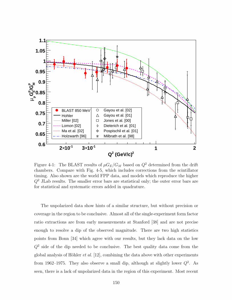
2 (GeV/c)2Q

-110×2 -110×3 1 2

p M/G

p EG

pµ

0.6

0.65

0.7

0.75

0.8

0.85

0.9

0.95

1

1.05

1.1

BLAST 850 MeVHohlerMiller [02]Lomon [02]Ma et al. [02]Holzwarth [96]

Gayou et al. [02]Gayou et al. [01]Jones et al. [00]Dieterich et al. [01]Pospischil et al. [01]Milbrath et al. [98]

Figure 4-1: The BLAST results of µGE/GM based on Q2 determined from the driftchambers. Compare with Fig. 4-5, which includes corrections from the scintillatortiming. Also shown are the world FPP data, and models which reproduce the higherQ2 JLab results. The smaller error bars are statistical only; the outer error bars arefor statistical and systematic errors added in quadrature.

The unpolarized data show hints of a similar structure, but without precision or

coverage in the region to be conclusive. Almost all of the single-experiment form factor

ratio extractions are from early measurements at Stanford [38] and are not precise

enough to resolve a dip of the observed magnitude. There are two high statistics

points from Bonn [34] which agree with our results, but they lack data on the low

Q2 side of the dip needed to be conclusive. The best quality data come from the

global analysis of Hohler et al. [12], combining the data above with other experiments

from 1962–1975. They also observe a small dip, although at slightly lower Q2. As

seen, there is a lack of unpolarized data in the region of this experiment. Most recent

150

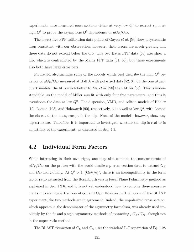
experiments have measured cross sections either at very low Q2 to extract rp or at

high Q2 to probe the asymptotic Q2 dependence of µGE/GM .

The lowest five FPP calibration data points of Gayou et al. [53] show a systematic

drop consistent with our observation; however, their errors are much greater, and

these data do not extend below the dip. The two Bates FPP data [50] also show a

dip, which is contradicted by the Mainz FPP data [51, 55], but these experiments

also both have large error bars.

Figure 4-1 also includes some of the models which best describe the high Q2 be-

havior of µGE/GM measured at Hall A with polarized data [52, 3]. Of the constituent

quark models, the fit is much better to Ma et al. [98] than Miller [86]. This is under-

standable, as the model of Miller was fit with only four free parameters, and thus it

overshoots the data at low Q2. The dispersion, VMD, and soliton models of Hohler

[12], Lomon [105], and Holzwarth [90], respectively, all do well at low Q2, with Lomon

the closest to the data, except in the dip. None of the models, however, show any

dip structure. Therefore, it is important to investigate whether the dip is real or is

an artifact of the experiment, as discussed in Sec. 4.3.

4.2 Individual Form Factors

While interesting in their own right, one may also combine the measurements of

µGE/GM on the proton with the world elastic e-p cross section data to extract GE

and GM individually. At Q2 > 1 (GeV/c)2, there is an incompatibility in the form

factor ratio extracted from the Rosenbluth versus Focal Plane Polarimetry method as

explained in Sec. 1.2.6, and it is not yet understood how to combine these measure-

ments into a single extraction of GE and GM . However, in the region of the BLAST

experiment, the two methods are in agreement. Indeed, the unpolarized cross section,

which appears in the denominator of the asymmetry formalism, was already used im-

plicitly by the fit and single-asymmetry methods of extracting µGE/GM , though not

in the super-ratio method.

The BLAST extraction of GE and GM uses the standard L-T separation of Eq. 1.28

151

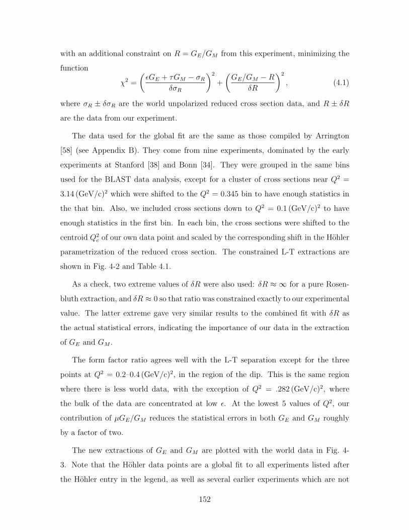
with an additional constraint on R = GE/GM from this experiment, minimizing the

function

χ2 =

(εGE + τGM − σR

δσR

)2

+

(GE/GM −R

δR

)2

, (4.1)

where σR ± δσR are the world unpolarized reduced cross section data, and R ± δR

are the data from our experiment.

The data used for the global fit are the same as those compiled by Arrington

[58] (see Appendix B). They come from nine experiments, dominated by the early

experiments at Stanford [38] and Bonn [34]. They were grouped in the same bins

used for the BLAST data analysis, except for a cluster of cross sections near Q2 =

3.14 (GeV/c)2 which were shifted to the Q2 = 0.345 bin to have enough statistics in

the that bin. Also, we included cross sections down to Q2 = 0.1 (GeV/c)2 to have

enough statistics in the first bin. In each bin, the cross sections were shifted to the

centroid Q2c of our own data point and scaled by the corresponding shift in the Hohler

parametrization of the reduced cross section. The constrained L-T extractions are

shown in Fig. 4-2 and Table 4.1.

As a check, two extreme values of δR were also used: δR ≈ ∞ for a pure Rosen-

bluth extraction, and δR ≈ 0 so that ratio was constrained exactly to our experimental

value. The latter extreme gave very similar results to the combined fit with δR as

the actual statistical errors, indicating the importance of our data in the extraction

of GE and GM .

The form factor ratio agrees well with the L-T separation except for the three

points at Q2 = 0.2–0.4 (GeV/c)2, in the region of the dip. This is the same region

where there is less world data, with the exception of Q2 = .282 (GeV/c)2, where

the bulk of the data are concentrated at low ε. At the lowest 5 values of Q2, our

contribution of µGE/GM reduces the statistical errors in both GE and GM roughly

by a factor of two.

The new extractions of GE and GM are plotted with the world data in Fig. 4-

3. Note that the Hohler data points are a global fit to all experiments listed after

the Hohler entry in the legend, as well as several earlier experiments which are not

152

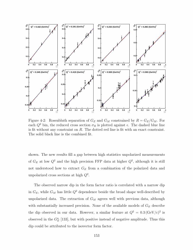
∈0 0.2 0.4 0.6 0.8 1

Rσ

0.2

0.3

0.4

0.5

2 = 0.162 (GeV/c)2Q

∈0 0.2 0.4 0.6 0.8 1

Rσ

0.2

0.3

0.4

0.5

2 = 0.191 (GeV/c)2Q

∈0 0.2 0.4 0.6 0.8 1

Rσ

0.2

0.3

0.4

0.5

2 = 0.232 (GeV/c)2Q

∈0 0.2 0.4 0.6 0.8 1

Rσ

0.2

0.3

0.4

2 = 0.282 (GeV/c)2Q

∈0 0.2 0.4 0.6 0.8 1

Rσ

0.15

0.2

0.25

0.3

2 = 0.345 (GeV/c)2Q

∈0 0.2 0.4 0.6 0.8 1

Rσ

0.15

0.2

0.25

0.3

2 = 0.419 (GeV/c)2Q

∈0 0.2 0.4 0.6 0.8 1

Rσ0.15

0.2

0.25

2 = 0.500 (GeV/c)2Q

∈0 0.2 0.4 0.6 0.8 1

Rσ

0.1

0.15

0.2

2 = 0.593 (GeV/c)2Q

Figure 4-2: Rosenbluth separation of GE and GM constrained by R = GE/GM . Foreach Q2 bin, the reduced cross section σR is plotted against ε. The dashed blue lineis fit without any constraint on R. The dotted red line is fit with an exact constraint.The solid black line is the combined fit.

shown. The new results fill a gap between high statistics unpolarized measurements

of GE at low Q2 and the high precision FFP data at higher Q2, although it is still

not understood how to extract GE from a combination of the polarized data and

unpolarized cross sections at high Q2.

The observed narrow dip in the form factor ratio is correlated with a narrow dip

in GE, while GM has little Q2 dependence beside the broad shape well-described by

unpolarized data. The extraction of GM agrees well with previous data, although

with substantially increased precision. None of the available models of GE describe

the dip observed in our data. However, a similar feature at Q2 = 0.3 (GeV/c)2 is

observed in the GnE [133], but with positive instead of negative amplitude. Thus this

dip could be attributed to the isovector form factor.

153

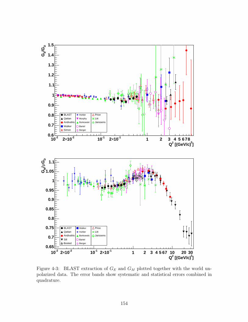
]2

[(GeV/c)2Q

-210 -210×2 -110 -110×2 1 2 3 4 5 6 78

D/G

EG

0.6

0.7

0.8

0.9

1

1.1

1.2

1.3

1.4

1.5

BLAST

Qattan

Andivahis

Walker

Simon

Hohler

Murphy

Borkowski

Bartel

Berger

Price

Litt

Janssens

]2

[(GeV/c)2Q

-210 -210×2 -110 -110×2 1 2 3 4 5 67 10 20 30

DGµ/

MG

0.65

0.7

0.75

0.8

0.85

0.9

0.95

1

1.05

1.1

BLAST

Qattan

Andivahis

Sill

Bosted

Walker

Hohler

Borkowski

Bartel

Berger

Price

Litt

Janssens

Figure 4-3: BLAST extraction of GE and GM plotted together with the world un-polarized data. The error bands show systematic and statistical errors combined inquadrature.

154

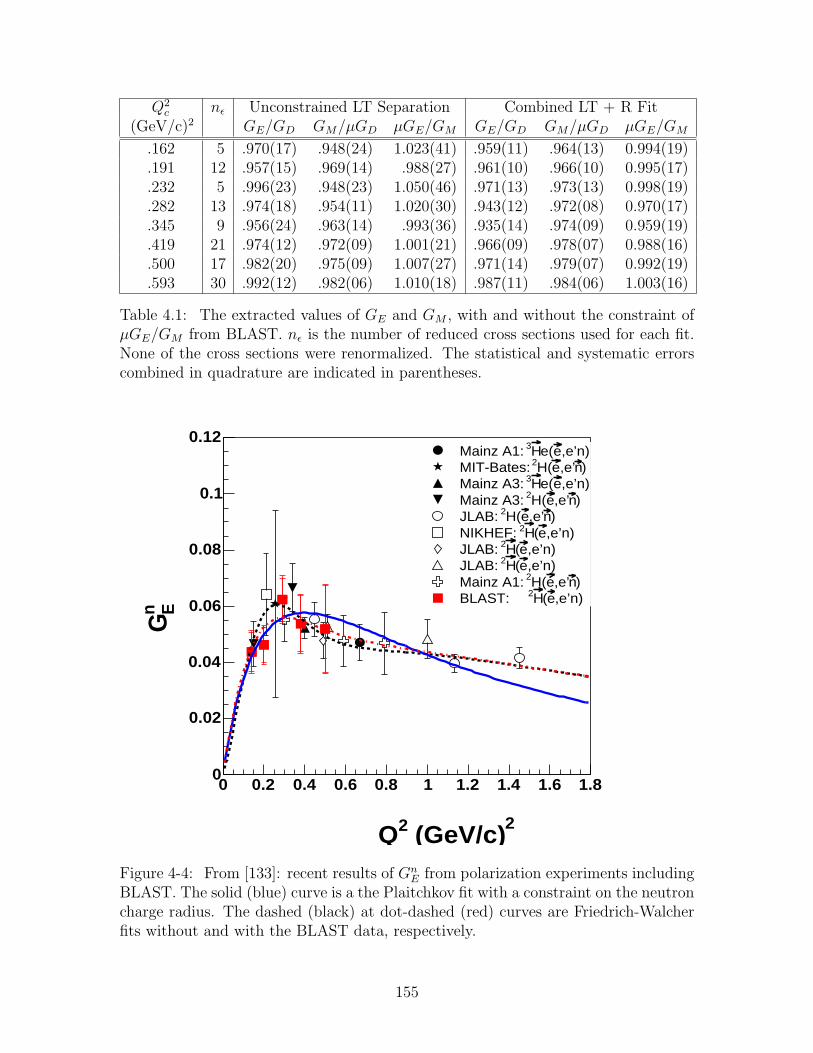
Q2c nε Unconstrained LT Separation Combined LT + R Fit

(GeV/c)2 GE/GD GM/µGD µGE/GM GE/GD GM/µGD µGE/GM

.162 5 .970(17) .948(24) 1.023(41) .959(11) .964(13) 0.994(19)

.191 12 .957(15) .969(14) .988(27) .961(10) .966(10) 0.995(17)

.232 5 .996(23) .948(23) 1.050(46) .971(13) .973(13) 0.998(19)

.282 13 .974(18) .954(11) 1.020(30) .943(12) .972(08) 0.970(17)

.345 9 .956(24) .963(14) .993(36) .935(14) .974(09) 0.959(19)

.419 21 .974(12) .972(09) 1.001(21) .966(09) .978(07) 0.988(16)

.500 17 .982(20) .975(09) 1.007(27) .971(14) .979(07) 0.992(19)

.593 30 .992(12) .982(06) 1.010(18) .987(11) .984(06) 1.003(16)

Table 4.1: The extracted values of GE and GM , with and without the constraint ofµGE/GM from BLAST. nε is the number of reduced cross sections used for each fit.None of the cross sections were renormalized. The statistical and systematic errorscombined in quadrature are indicated in parentheses.

0 0.2 0.4 0.6 0.8 1 1.2 1.4 1.6 1.80

0.02

0.04

0.06

0.08

0.1

0.12,e’n)ee(H3Mainz A1:

)n,e’eH(2MIT-Bates: ,e’n)ee(H3Mainz A3:

)n,e’eH(2Mainz A3: )n,e’eH(2JLAB:

,e’n)e(H2NIKHEF: ,e’n)e(H2JLAB: ,e’n)e(H2JLAB:

)n,e’eH(2Mainz A1: ,e’n)e(H2BLAST:

2 (GeV/c)2Q

EnG

Figure 4-4: From [133]: recent results of GnE from polarization experiments including

BLAST. The solid (blue) curve is a the Plaitchkov fit with a constraint on the neutroncharge radius. The dashed (black) at dot-dashed (red) curves are Friedrich-Walcherfits without and with the BLAST data, respectively.

155

4.3 Discussion of Errors

We now return to the question of whether the observed dip is physical or is an artifact

of the experiment. First consider statistical errors from drift chamber reconstruction

only. We group the data in three sets: the first three points before the dip, the next

two points in the dip, and the last three points after the dip. The average form factor

ratio in these sets is µGE/GM = 0.9887±0.0069, 0.9429±0.0088, and 0.9708±0.0110

respectively. The weighted difference between the average form factor ratio of the two

middle points and the rest of the data is 0.0407±0.0106. Thus without consideration

of systematic errors the dip is a 4σ effect.

A few checks were performed to ensure that the data were normally distributed

and the the dip was not an anomaly. All three methods of the extracting the form

factor ratio reproduce the dip. The single-asymmetry extraction and the global fit

extraction are very close to each other at all Q2 points. The super-ratio method

extraction differs from the other two methods by 1.5σ at Q2 = 0.345 and 0.592. The

extracted polarization also differs by the same amount at those points, indicating

that there is a discrepancy between the left and right asymmetries at these points.

But the super-ratio extraction of µGE/GM is in agreement with the other methods

at Q2 = 0.282, the first point of the dip.

As discussed in Sec. 3.1.4, the efficiency of the left sector TOF paddle 9 changed

twice during the experiment, potentially affecting the asymmetry at Q2 = 0.282.

However, the asymmetry and form factor ratio were analyzed in six sequential run

periods (Fig. 3-17), and all periods were consistent with each other. The data were

also analyzed in finer Q2 bins in Fig. 3-16, and a dip was still observed in four bins.

There we concluded that statistically, the dip is real.

Some of the systematic errors are overall normalization uncertainties, affecting

µGE/GM at each Q2 by the same amount. These have no effect on the presence

of a dip. For example, a one degree overestimation of the average target spin angle

would raise µGE/GM by 0.0073. False asymmetries due to improper beam current

integration, or asymmetries in beam or target helicity states would also have the same

156

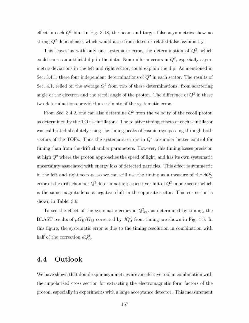
effect in each Q2 bin. In Fig. 3-18, the beam and target false asymmetries show no

strong Q2 dependence, which would arise from detector-related false asymmetry.

This leaves us with only one systematic error, the determination of Q2, which

could cause an artificial dip in the data. Non-uniform errors in Q2, especially asym-

metric deviations in the left and right sector, could explain the dip. As mentioned in

Sec. 3.4.1, there four independent determinations of Q2 in each sector. The results of

Sec. 4.1, relied on the average Q2 from two of these determinations: from scattering

angle of the electron and the recoil angle of the proton. The difference of Q2 in these

two determinations provided an estimate of the systematic error.

From Sec. 3.4.2, one can also determine Q2 from the velocity of the recoil proton

as determined by the TOF scintillators. The relative timing offsets of each scintillator

was calibrated absolutely using the timing peaks of cosmic rays passing through both

sectors of the TOFs. Thus the systematic errors in Q2 are under better control for

timing than from the drift chamber parameters. However, this timing losses precision

at high Q2 where the proton approaches the speed of light, and has its own systematic

uncertainty associated with energy loss of detected particles. This effect is symmetric

in the left and right sectors, so we can still use the timing as a measure of the dQ2A

error of the drift chamber Q2 determination; a positive shift of Q2 in one sector which

is the same magnitude as a negative shift in the opposite sector. This correction is

shown in Table. 3.6.

To see the effect of the systematic errors in Q2WC as determined by timing, the

BLAST results of µGE/GM corrected by dQ2A from timing are shown in Fig. 4-5. In

this figure, the systematic error is due to the timing resolution in combination with

half of the correction dQ2A.

4.4 Outlook

We have shown that double spin-asymmetries are an effective tool in combination with

the unpolarized cross section for extracting the electromagnetic form factors of the

proton, especially in experiments with a large acceptance detector. This measurement

157

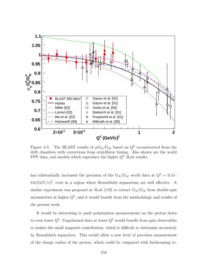
2 (GeV/c)2Q

-110×2 -110×3 1 2

p M/G

p EG

pµ

0.6

0.65

0.7

0.75

0.8

0.85

0.9

0.95

1

1.05

1.1

BLAST 850 MeVHohlerMiller [02]Lomon [02]Ma et al. [02]Holzwarth [96]

Gayou et al. [02]Gayou et al. [01]Jones et al. [00]Dieterich et al. [01]Pospischil et al. [01]Milbrath et al. [98]

Figure 4-5: The BLAST results of µGE/GM based on Q2 reconstructed from thedrift chambers with corrections from scintillator timing. Also shown are the worldFPP data, and models which reproduce the higher Q2 JLab results.

has substantially increased the precision of the GE/GM world data at Q2 = 0.15–

0.6 (GeV/c)2, even in a region where Rosenbluth separations are still effective. A

similar experiment was proposed at JLab [119] to extract GE/GM from double-spin

asymmetries at higher Q2, and it would benefit from the methodology and results of

the present work.

It would be interesting to push polarization measurements on the proton down

to even lower Q2. Unpolarized data at lower Q2 would benefit from spin observables

to isolate the small magnetic contribution, which is difficult to determine accurately

by Rosenbluth separation. This would allow a new level of precision measurement

of the charge radius of the proton, which could be compared with forthcoming re-

158

sults of the muonic hydrogen Lamb shift experiment [29]. One could also perform a

quality extraction of the magnetic radius of the proton, which is poorly known with

unpolarized data alone.

The significance of this measurement is still limited by systematic errors mainly in

the determination of Q2 and the holding field angle β. Reduction of the uncertainty

of Q2 is important, since this is the only systematic error which could be responsible

for the observed dip in µGE/GM if it is unphysical. The extraction process is highly

sensitive to Q2 even though the form factors are fairly constant in Q2. There are con-

tributions from both the Q2 dependence of the asymmetry, and from the uncertainty

in θ∗ and kinematic factors. The first contribution is most serious, especially if the left

and right sectors of BLAST are asymmetric such that the error in Q2 is different in

both sectors. There are indications from comparisons of independent measurements

of Q2 in each sector that this is indeed the case.

In order to resolve the discrepancy of Q2, an absolute calibration of the wire

chambers is needed. All available information from the experimental data, cosmic

rays, and detector surveys must be used to get a consistent calibration of the drift

chambers. After the current physics run, the BLAST magnetic field will be measured

with the target and all of the outer detectors in place and compared with the previous

field map and TOSCA calculations. Extra cosmic ray data will also be taken at this

time with zero magnetic field. These straight tracks will be useful for investigating

the relative alignment of the three chambers within a sector and of one sector relative

to the other. There may even be sufficient cosmic events in the existing physics data,

although the wire chamber requirements in the trigger may be too restrictive.

After the most recent map of target holding field, the target polarization angle is

reasonably well-known, and agrees well with the angle extracted from the data. Work

is underway to increase the precision of the field map to less than 0.5 at the end of

the current run, which will make the uncertainty in θ∗ insignificant. By accomplishing

the above tasks, it will be possible to reduce the systematic errors to the level of the

statistical errors of this experiment.

While there is a great push to understand the recently discovered drop in GE

159

at high Q2 in terms of the dynamics of constituent quarks, and also to reconcile

Rosenbluth and Focal Plane Polarimeter extractions of µGE/GM in terms of higher

order radiative corrections, there are also interesting features in the Q2 range of this

work. The first steps have been taken by Friedrich and Walcher [60] to parametrize

the meson cloud of the nucleon by phenomenological fits of the low Q2 dependence

of the form factors. There is an opportunity to extend this investigation with more

physical models.

If the observed dip in µGE/GM turns out to be physical after reducing the system-

atic error in Q2 and comparing the results with an analysis of the BLAST deuterium

data, it would be a signature which could be tested against new models of the nucleon

and direct calculations of Lattice QCD. This region is too high in Q2 for effective field

theories, but it would be interesting if they could reproduce similar features. Its effect

on the nucleon-nucleon potential would also be interesting. These results are another

piece of the puzzle in understanding hadronic structure in terms of the underlying

quark and gluon degrees of freedom.

160

Appendix A

Linear Calibrations

Although some calibrations of the BLAST detector can be done with single measure-

ments, for example using the flashers, additional information is available by consider-

ing physically motivated correlations between detector signals. In this appendix, we

use such correlations to calibrate the TOF scintillator timing offsets and the time-

to-distance function for wires in the drift chambers. Many of the correlations are

linear or can be approximated by a linear function in the region of the calibration,

which greatly simplifies the solution. We first review the formalism of linear least

squares fitting based on the treatment in Numerical Recipes [150, §15], and discuss

the robust fitting of multivariate correlations. This is applied to calibrations in the

following sections.

A.1 Least Squares Fit

The least squares fit of data points (xi, yi) to the straight line y = mx+ b is obtained

by minimizing the sum of squared deviations

χ2 =∑

i

(yi −mxi − b)2 = (Y −Xa)2, (A.1)

161

where the data and parameters are represented by the matrices

Y =

y1

y2

...

, X =

x1 1

x2 1...

...

, a =

(m

b

). (A.2)

The design matrix X is composed of rows of the coefficients of m and b for each data

point. This can be generalized to any fit function which is linear in the fit parameters,

y =∑

j Xj(x)aj, in which case the design matrix has components Xij = Xj(xi). The

domain xi is arbitrary (discrete, continuous, vector space, or manifold). The range

yi must be continuous, and if it is a vector space, X and Y are segmented into

block rows containing the vector components of each data point. The minimum of χ2

with respect to the parameters a has the solution

dχ2|min = 2 daT XT (Y −Xa) = 0, (A.3)

XT Y = XT Xa, (A.4)

a = XaY where Xa ≡ (XT X)−1XT . (A.5)

The matrix Xa is defined as the least squares left sided inverse of X.

If the data points have Gaussian errors yi±∆yi, then the maximum likelihood fit

is obtained by minimizing the chi-squared variable

χ2 =∑

i

(yi −mxi − b

∆yi

)2

= (Y −Xa)2. (A.6)

Each row of X and Y is divided by ∆yi, and the solution has the same form. The

covariance matrix C of a has components

Cij = Cov(ai, aj) =∑

k

(∆yk

2 ∂ai

∂yk

∂aj

∂yk

= XaikX

ajk

)= (XT X)−1

ij. (A.7)

The design matrix does not have to be constructed from a single fit function of

homogeneous data, but can be formed of arbitrary linear (or linearized) equations in

162

the fit parameters. Thus one can fit subsets of the data separately using individualized

techniques and combine the results into a global linear fit, weighted by the errors in

each subset of the data. The resulting system of weighted linear equations, Y = Xa,

has the same form as above with the same least squares solution. This is the technique

used in calibrating the TOF offsets (Sec. A.2) and the drift chamber wire time-to-

distance functions (Sec. A.3.3).

Singular Value Decomposition (SVD)

Alternatively, one can compute the least squares inverse robustly by calculating the

SVD [150, §2.6]. The matrix X can be decomposed as X = RPS into a rota-

tion R, a projection P , and a symmetric matrix S, which has the further decom-

position S = V WV T with eigenvalues W = diag(w1, w2, . . . , wn) and eigenvectors

V = (V1|V2| . . . |Vn). Setting U = RPV (with the same dimensions as X and P ),

X = UWV T and Xa = V W−1UT , (A.8)

where U is orthonormal, V is a rotation, and W is diagonal. The least squares fit has

the solution

a = XaY =∑

k

VkUk · Y ± 1

wk

, (A.9)

where ±1 indicates the uncertainty in a with each term added in quadrature, since C

is diagonal in the basis Vk. In the case of a linear fit with x = 0, the two columns

of X are already orthogonal and V = 1. For large datasets where is it impractical to

tabulate X, one can calculate the SVD of XT X instead.

A.1.1 Generalizations of the Linear Fit

Consider multiple data points at a single of value x, and note that individual rows of

X and Y can be added separately to XTX and XTY , weighted by ∆y−2i . Therefore, it

is equivalent to replace these rows with a single row of the average y where y/∆y2 ≡∑i yi/∆y2

i , weighted by ∆y−2 ≡∑

i ∆y−2i . The importance of this observation is that

163

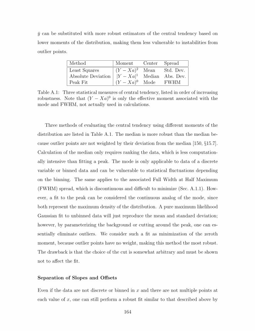
y can be substituted with more robust estimators of the central tendency based on

lower moments of the distribution, making them less vulnerable to instabilities from

outlier points.

Method Moment Center Spread

Least Squares (Y −Xa)2 Mean Std. Dev.Absolute Deviation |Y −Xa|1 Median Abs. Dev.Peak Fit (Y −Xa)0 Mode FWHM

Table A.1: Three statistical measures of central tendency, listed in order of increasingrobustness. Note that (Y − Xa)0 is only the effective moment associated with themode and FWHM, not actually used in calculations.

Three methods of evaluating the central tendency using different moments of the

distribution are listed in Table A.1. The median is more robust than the median be-

cause outlier points are not weighted by their deviation from the median [150, §15.7].

Calculation of the median only requires ranking the data, which is less computation-

ally intensive than fitting a peak. The mode is only applicable to data of a discrete

variable or binned data and can be vulnerable to statistical fluctuations depending

on the binning. The same applies to the associated Full Width at Half Maximum

(FWHM) spread, which is discontinuous and difficult to minimize (Sec. A.1.1). How-

ever, a fit to the peak can be considered the continuous analog of the mode, since

both represent the maximum density of the distribution. A pure maximum likelihood

Gaussian fit to unbinned data will just reproduce the mean and standard deviation;

however, by parameterizing the background or cutting around the peak, one can es-

sentially eliminate outliers. We consider such a fit as minimization of the zeroth

moment, because outlier points have no weight, making this method the most robust.

The drawback is that the choice of the cut is somewhat arbitrary and must be shown

not to affect the fit.

Separation of Slopes and Offsets

Even if the data are not discrete or binned in x and there are not multiple points at

each value of x, one can still perform a robust fit similar to that described above by

164

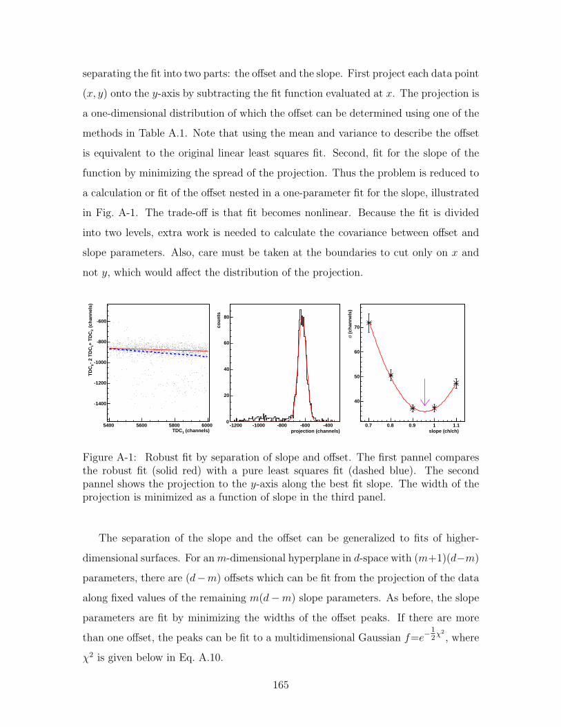
separating the fit into two parts: the offset and the slope. First project each data point

(x, y) onto the y-axis by subtracting the fit function evaluated at x. The projection is

a one-dimensional distribution of which the offset can be determined using one of the

methods in Table A.1. Note that using the mean and variance to describe the offset

is equivalent to the original linear least squares fit. Second, fit for the slope of the

function by minimizing the spread of the projection. Thus the problem is reduced to

a calculation or fit of the offset nested in a one-parameter fit for the slope, illustrated

in Fig. A-1. The trade-off is that fit becomes nonlinear. Because the fit is divided

into two levels, extra work is needed to calculate the covariance between offset and

slope parameters. Also, care must be taken at the boundaries to cut only on x and

not y, which would affect the distribution of the projection.

(channels)1TDC5400 5600 5800 6000

(ch

ann

els)

2+

TD

C1

- 2

TD

C0

TD

C

-1400

-1200

-1000

-800

-600

projection (channels)-1200 -1000 -800 -600 -400

cou

nts

0

20

40

60

80

slope (ch/ch) 0.7 0.8 0.9 1 1.1

(ch

ann

els)

σ

40

50

60

70

Figure A-1: Robust fit by separation of slope and offset. The first pannel comparesthe robust fit (solid red) with a pure least squares fit (dashed blue). The secondpannel shows the projection to the y-axis along the best fit slope. The width of theprojection is minimized as a function of slope in the third panel.

The separation of the slope and the offset can be generalized to fits of higher-

dimensional surfaces. For an m-dimensional hyperplane in d-space with (m+1)(d−m)

parameters, there are (d−m) offsets which can be fit from the projection of the data

along fixed values of the remaining m(d−m) slope parameters. As before, the slope

parameters are fit by minimizing the widths of the offset peaks. If there are more

than one offset, the peaks can be fit to a multidimensional Gaussian f=e−12

χ2

, where

χ2 is given below in Eq. A.10.

165

The slope parameters can be determined by calculating χ2 (width of the offsets

projection) for each point on a grid of the slope parameters a and fitting for the

minimum a0. Near a0, the function χ2 can be fit to the quadratic form

χ2 = aT Aa + aT b + c (A.10)

= (a− a0)T A(a− a0) + aT (b + 2Aa0) + (c− aT

0 Aa0) (A.11)

with the new parameters grouped into a symmetric matrix A, a vector b, and a scalar

c. In terms of these parameters, the minimum is

χ2min = c + 1

2bTa0 at a0 = −1

2A−1b. (A.12)

The covariance matrix for the slope parameters is C = A−1 if the width of the

projection χ2 has been normalized by ∆yi. Otherwise, the best one can do is scale

χ2min to equal (d−m), resulting in the covariance matrix C = A−1χ2

min/(d−m).

A nonlinear parametrized m-dimensional surface S can also be fit using this

method. The surface is re-parametrized to have (d − m) offsets plus the remain-

ing shape (slope) parameters by considering the intersection of S with a (d − m)

hyperplane extending out from a fixed point on the original surface. For the sur-

face of a two-dimensional function f(x, y; ai) with parameters ai, the natural offset

parameter is z = f(0, 0; ai), and the data point (x, y, z) is projected onto the z-axis

by subtracting f(x, y; ai). After adding the offset parameter z, one of the shape

parameters ai will be redundant and must be excluded from the fit.

A.1.2 Minimum χ2 from a Least Squares Fit

Returning to the linear least squares fit, we substitute in the fitted value of a to get

χ2min = (Y −XXaY )2 = Y T P⊥Y (A.13)

= Y TY − Y TX (XTX)−1XTY, (A.14)

166

where P‖ ≡ XXa = UUT = P 2‖ is the 2-dimensional projection of points yi onto the

fitted line, and P⊥ = 1 − P‖ = P 2⊥ is the (n − 2) dimensional projection onto the

residuals of yi contributing to χ2. Substituting averages for Y T Y , Y T X, and XT X,

1nχ2

min = y2 − ( yx y )

x2 − x2

(1 −x

−x x2

)(yx

y

)(A.15)

= (y2 − y2)− (yx− y x)2/(x2 − x2) (A.16)

= Var(y)− Cov(y, x)2/Var(x) (A.17)

= Var(y)(1− r2), (A.18)

where Var(x) ≡ (x− x)2 = x2 − x2 and Cov(y, x) ≡ yx − x y are the variance and

covariance respectively, and the linear correlation r is defined by

r ≡ Cov(y, x)√Var(y)Var(x)

. (A.19)

For the case n = 2, the fit is exact and χ2min = 0. For the case n = 3, using data

points (−x, y1), (0, y2), and (x, y3),

χ2min =

∑y2 − 1

n(∑

y)2 − (∑

xy)2/∑

x2 (A.20)

= (y21 + y2

2 + y23)− 1

3(y1 + y2 + y3)

2 − 12(y3 − y1)

2 (A.21)

= 16(y1 − 2y2 + y3)

2. (A.22)

Intuitively, this is the difference between the average of the two outer points and the

middle point, which would coincide for an exact fit.

We now consider the SVD to show that in general χ2min is the sum of (n − 2)

squares. It is apparent from equation A.13 that

χ2min = Y T (1− UUT )Y = (U3 · Y )2 + (U4 · Y )2 + . . . + (Un · Y )2, (A.23)

where U = (U1|U2) has only the two eigenvectors of P‖. To get the (n−2) eigenvectors

of the complement, pad X with null vectors before computing the SVD or complete

167

U to a full basis using the Gram-Schmidt process. Again, for the case n = 3, the

third eigenvector is U3 = 1√6(1,−2, 1). For the case n = 4, with regularly space points

in x, the design matrix

XT =

(−3 −1 1 3

1 1 1 1

)(A.24)

is completed with the null eigenvectors U3 = 12(1,−1,−1, 1) and U4 = 1√

20(1,−3, 3,−1)

or linear combinations thereof. Therefore,

χ2min = 1

4(y1 − y2 − y3 + y4)

2 + 120

(y1 − 3y2 + 3y3 − y4)2. (A.25)

The first term is the difference in averages between the outer and inner points, while

the second term is the difference between averages of y1, y3, and y2, y4, weighted

to meet at the center. These formulas are useful for bypassing the fit process and

directly computing how well hits in a track line up, for example. They are used in

the linear calibration of the drift chamber time-to-distance functions.

A.2 TOF Scintillator Offsets

As described in Secs. 2.3.3 and 3.1.1, there are 16 TOF scintillators (n=0–15) in each

sector (s=L,R). The TDC values from the top and bottom PMTs are labeled usn and

dsn, respectively. The two PMTs allow the measurement of both the mean time tsn

and position psn along the length of the scintillator of each hit,

tsn = 12(ds

n + usn)tch (A.26)

psn = 1

2(ds

n − usn)tchvsc, (A.27)

where vsc ≈ 14.7 cm/ns is the velocity of light in the scintillator, accounting for

the average number of reflections before being detected in the PMT, and calibrated

by matching the range of psn to thed length of the scintillator. The TDC channel

resolution tch ≈ 50 ps/ch was calibrated by adding predetermined delays to the

signals from each PMT and measuring corresponding delays in the TDC channels.

168

Each TDC has an offset which includes the intrinsic offset of TDC electronics and

delays from light propagation in the scintillator, cable, and trigger logic,

xsn = xs

n raw− xs

n offwhere x = d, u, t, p. (A.28)

The offsets dsn off

and usn off

were measured with the flasher as described in Sec. 2.3.3.

However, some flasher signals were missing due to attenuation and broken fibers,

and this was not an absolute calibration, since not all fiber optics were the same

length (due to an extra splitter box) and they were not all placed exactly in center

of detector. An absolute calibration of the offsets was accomplished using cosmic ray

coincidence events and the coplanarity the elastic ep events, described in the next

two sections.

A.2.1 Cosmic Coincidences

The mean time offset tsn offof each paddle was calibrated absolutely using cosmic rays

at low enough zenith angle Θ to pass through both a scintillator in the left sector

and one in the right sector, triggering a coincidence event. Although the cosmic

radiation is predominantly vertical and the distribution decreases as cos(Θ), the rate

of coincident events (1.4 Hz) was large enough for an accurate calibration of the

timing offsets with only a few hours of data, taken periodically during maintenance

of the SHR. The cosmic rays are predominantly high energy muons traveling near

the speed of light, so the time delay between two TOF signals only depends on the

distance between TOFs and it is reasonable to assume that left and right directions

have same velocity distribution.

The distribution tRi − tLj has two peaks, Lij and Rij, corresponding to cosmic rays

traveling to the left and right, respectively. The peaks were enhanced by correcting

for zenith angle Θ of the particle. From these two peaks we get the distance Dij

between the two scintillators, and the difference Sij between the left and right offsets,

Dij = ctch(Rij − Lij) (A.29)

169

Sij = 12(Rij + Lij). (A.30)

Let the li and ri be the offsets of each scintillator in the left and right sector, respec-

tively, then the 16× 16 equations

√Nij(Sij = ri − lj) (A.31)

overdetermine each offset up to a global offset, which is insignificant because all

timing in the BLAST detector is relative. The offsets are determined by a least

squares solution to the above system of equations (Sec. A.1), each weighted by the

number of events NR,Lij in each peak as

σ2 ∝ 1Nij

≡ 1NR

ij+ 1

NLij, (A.32)

The degeneracy of the undetermined global offset is removed by setting it to zero

with the additional equations

√NR

i (ri = SRi = 0) and

√NL

i (li = SLi = 0) (A.33)

with very low weights NL,Ri = 10−3. Following Sec. A.1, with a = (r0, . . . , r15, l0, . . . , l15)

and the rows of X and Y formed from Eqs. A.31 and A.33, we obtain from Eq. A.4

the block matrix equation (A B

C D

)(l

r

)=

(E

F

)(A.34)

with components

Aij = δij(∑

k Nik + NRi ), Bij = −Nij, Ei =

∑k NikSik + NR

i SRi ,

Dij = δij(∑

k Nkj + NLj ), Cij = −Nji, Fi =

∑k NkjSkj + NL

j SLj ,

(A.35)

which can be solved for the offsets li and ri.

This procedure was used by the ROOT macro tmt_offsets.C to calculate the

170

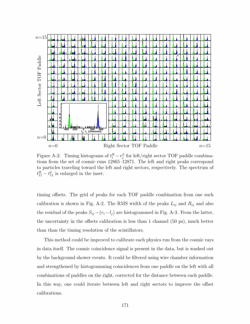
(channels) L- tR

t-400 -200 0 200 400

02468

n=15

n=0

n=0 n=15Right Sector TOF Paddle

Lef

tSec

tor

TO

FPad

dle

Figure A-2: Timing histograms of tRi − rLj for left/right sector TOF paddle combina-

tions from the set of cosmic runs 12865–12871. The left and right peaks correspondto particles traveling toward the left and right sectors, respectively. The spectrum oftR11 − tL11 is enlarged in the inset.

timing offsets. The grid of peaks for each TOF paddle combination from one such

calibration is shown in Fig. A-2. The RMS width of the peaks Lij and Rij and also

the residual of the peaks Sij−(ri− lj) are histogrammed in Fig. A-3. From the latter,

the uncertainty in the offsets calibration is less than 1 channel (50 ps), much better

than than the timing resolution of the scintillators.

This method could be improved to calibrate each physics run from the cosmic rays

in data itself. The cosmic coincidence signal is present in the data, but is washed out

by the background shower events. It could be filtered using wire chamber information

and strengthened by histogramming coincidences from one paddle on the left with all

combinations of paddles on the right, corrected for the distance between each paddle.

In this way, one could iterate between left and right sectors to improve the offset

calibrations.

171

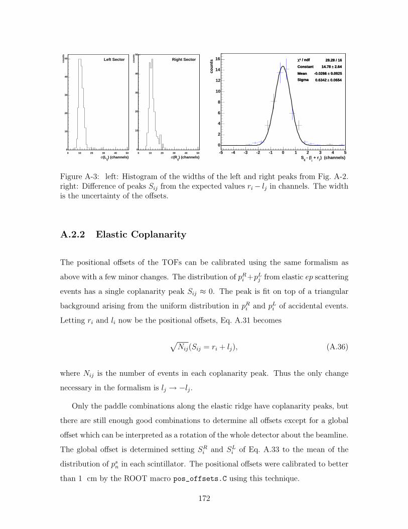
) (channels)ij

(Lσ0 10 20 30 40 50

cou

nts

0

10

20

30

40

50 Left Sector

) (channels)ij

(Rσ0 10 20 30 40 50

cou

nts

0

10

20

30

40

50

Right Sector / ndf 2χ 28.28 / 16

Constant 2.64± 14.78

Mean 0.0925± -0.0266

Sigma 0.0654± 0.6342

) (channels)j + ri

- (lijS-5 -4 -3 -2 -1 0 1 2 3 4 5

cou

nts

0

2

4

6

8

10

12

14

16 / ndf 2χ 28.28 / 16

Constant 2.64± 14.78

Mean 0.0925± -0.0266

Sigma 0.0654± 0.6342

Figure A-3: left: Histogram of the widths of the left and right peaks from Fig. A-2.right: Difference of peaks Sij from the expected values ri− lj in channels. The widthis the uncertainty of the offsets.

A.2.2 Elastic Coplanarity

The positional offsets of the TOFs can be calibrated using the same formalism as

above with a few minor changes. The distribution of pRi +pL

j from elastic ep scattering

events has a single coplanarity peak Sij ≈ 0. The peak is fit on top of a triangular

background arising from the uniform distribution in pRi and pL

i of accidental events.

Letting ri and li now be the positional offsets, Eq. A.31 becomes

√Nij(Sij = ri + lj), (A.36)

where Nij is the number of events in each coplanarity peak. Thus the only change

necessary in the formalism is lj → −lj.

Only the paddle combinations along the elastic ridge have coplanarity peaks, but

there are still enough good combinations to determine all offsets except for a global

offset which can be interpreted as a rotation of the whole detector about the beamline.

The global offset is determined setting SRi and SL

i of Eq. A.33 to the mean of the

distribution of psn in each scintillator. The positional offsets were calibrated to better

than 1 cm by the ROOT macro pos_offsets.C using this technique.

172

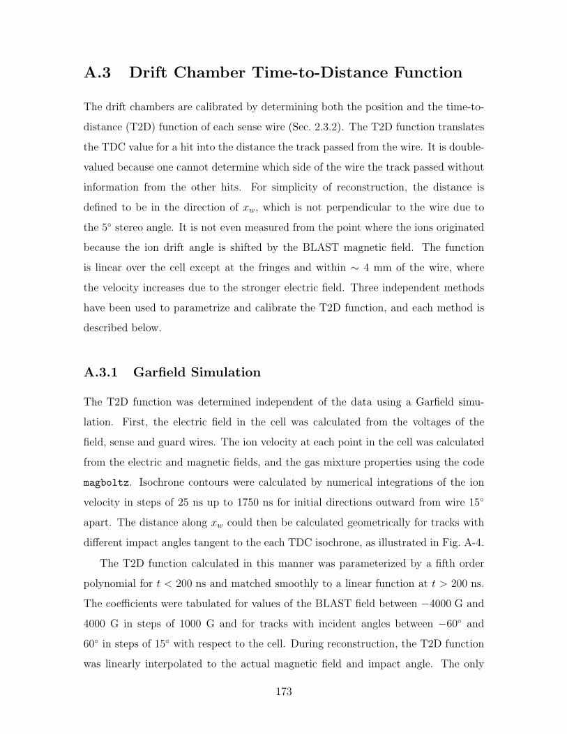
A.3 Drift Chamber Time-to-Distance Function

The drift chambers are calibrated by determining both the position and the time-to-

distance (T2D) function of each sense wire (Sec. 2.3.2). The T2D function translates

the TDC value for a hit into the distance the track passed from the wire. It is double-

valued because one cannot determine which side of the wire the track passed without

information from the other hits. For simplicity of reconstruction, the distance is

defined to be in the direction of xw, which is not perpendicular to the wire due to

the 5 stereo angle. It is not even measured from the point where the ions originated

because the ion drift angle is shifted by the BLAST magnetic field. The function

is linear over the cell except at the fringes and within ∼ 4 mm of the wire, where

the velocity increases due to the stronger electric field. Three independent methods

have been used to parametrize and calibrate the T2D function, and each method is

described below.

A.3.1 Garfield Simulation

The T2D function was determined independent of the data using a Garfield simu-

lation. First, the electric field in the cell was calculated from the voltages of the

field, sense and guard wires. The ion velocity at each point in the cell was calculated

from the electric and magnetic fields, and the gas mixture properties using the code

magboltz. Isochrone contours were calculated by numerical integrations of the ion

velocity in steps of 25 ns up to 1750 ns for initial directions outward from wire 15

apart. The distance along xw could then be calculated geometrically for tracks with

different impact angles tangent to the each TDC isochrone, as illustrated in Fig. A-4.

The T2D function calculated in this manner was parameterized by a fifth order

polynomial for t < 200 ns and matched smoothly to a linear function at t > 200 ns.

The coefficients were tabulated for values of the BLAST field between −4000 G and

4000 G in steps of 1000 G and for tracks with incident angles between −60 and

60 in steps of 15 with respect to the cell. During reconstruction, the T2D function

was linearly interpolated to the actual magnetic field and impact angle. The only

173

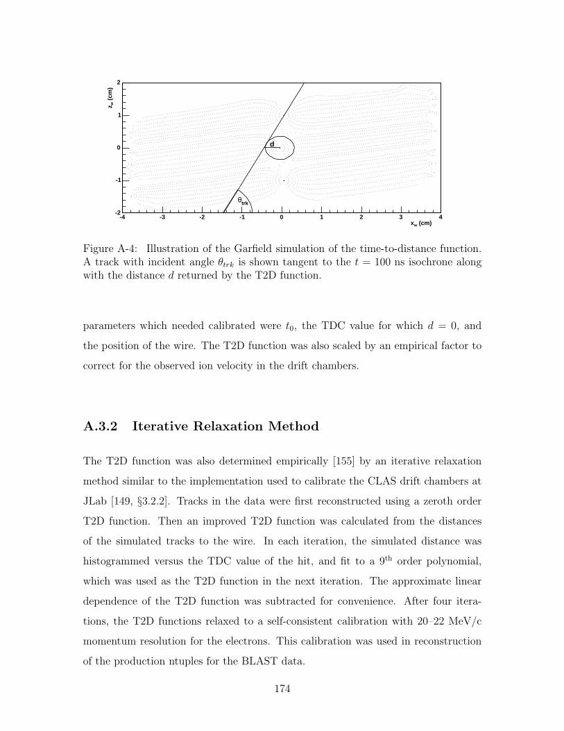
(cm) wx-4 -3 -2 -1 0 1 2 3 4

(cm

)

wz

-2

-1

0

1

2

d

trkθ

Figure A-4: Illustration of the Garfield simulation of the time-to-distance function.A track with incident angle θtrk is shown tangent to the t = 100 ns isochrone alongwith the distance d returned by the T2D function.

parameters which needed calibrated were t0, the TDC value for which d = 0, and

the position of the wire. The T2D function was also scaled by an empirical factor to

correct for the observed ion velocity in the drift chambers.

A.3.2 Iterative Relaxation Method

The T2D function was also determined empirically [155] by an iterative relaxation

method similar to the implementation used to calibrate the CLAS drift chambers at

JLab [149, §3.2.2]. Tracks in the data were first reconstructed using a zeroth order

T2D function. Then an improved T2D function was calculated from the distances

of the simulated tracks to the wire. In each iteration, the simulated distance was

histogrammed versus the TDC value of the hit, and fit to a 9th order polynomial,

which was used as the T2D function in the next iteration. The approximate linear

dependence of the T2D function was subtracted for convenience. After four itera-

tions, the T2D functions relaxed to a self-consistent calibration with 20–22 MeV/c

momentum resolution for the electrons. This calibration was used in reconstruction

of the production ntuples for the BLAST data.

174

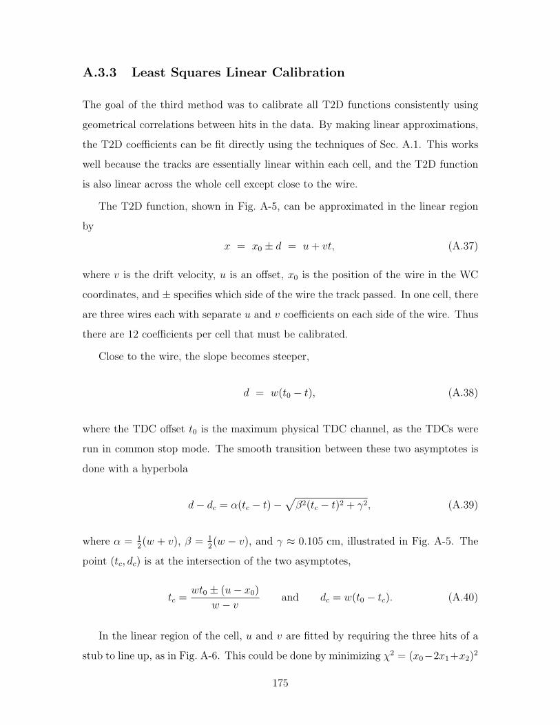
A.3.3 Least Squares Linear Calibration

The goal of the third method was to calibrate all T2D functions consistently using

geometrical correlations between hits in the data. By making linear approximations,

the T2D coefficients can be fit directly using the techniques of Sec. A.1. This works

well because the tracks are essentially linear within each cell, and the T2D function

is also linear across the whole cell except close to the wire.

The T2D function, shown in Fig. A-5, can be approximated in the linear region

by

x = x0 ± d = u + vt, (A.37)

where v is the drift velocity, u is an offset, x0 is the position of the wire in the WC

coordinates, and ± specifies which side of the wire the track passed. In one cell, there

are three wires each with separate u and v coefficients on each side of the wire. Thus

there are 12 coefficients per cell that must be calibrated.

Close to the wire, the slope becomes steeper,

d = w(t0 − t), (A.38)

where the TDC offset t0 is the maximum physical TDC channel, as the TDCs were

run in common stop mode. The smooth transition between these two asymptotes is

done with a hyperbola

d− dc = α(tc − t)−√

β2(tc − t)2 + γ2, (A.39)

where α = 12(w + v), β = 1

2(w − v), and γ ≈ 0.105 cm, illustrated in Fig. A-5. The

point (tc, dc) is at the intersection of the two asymptotes,

tc =wt0 ± (u− x0)

w − vand dc = w(t0 − tc). (A.40)

In the linear region of the cell, u and v are fitted by requiring the three hits of a

stub to line up, as in Fig. A-6. This could be done by minimizing χ2 = (x0−2x1+x2)2

175

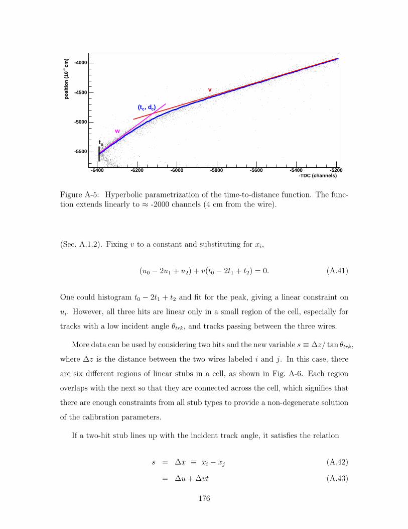
-TDC (channels) -6400 -6200 -6000 -5800 -5600 -5400 -5200

cm

)

-3

po

siti

on

(10

-5500

-5000

-4500

-4000

0t

)c, dc(t

w

v

Figure A-5: Hyperbolic parametrization of the time-to-distance function. The func-tion extends linearly to ≈ -2000 channels (4 cm from the wire).

(Sec. A.1.2). Fixing v to a constant and substituting for xi,

(u0 − 2u1 + u2) + v(t0 − 2t1 + t2) = 0. (A.41)

One could histogram t0 − 2t1 + t2 and fit for the peak, giving a linear constraint on

ui. However, all three hits are linear only in a small region of the cell, especially for

tracks with a low incident angle θtrk, and tracks passing between the three wires.

More data can be used by considering two hits and the new variable s ≡ ∆z/ tan θtrk,

where ∆z is the distance between the two wires labeled i and j. In this case, there

are six different regions of linear stubs in a cell, as shown in Fig. A-6. Each region

overlaps with the next so that they are connected across the cell, which signifies that

there are enough constraints from all stub types to provide a non-degenerate solution

of the calibration parameters.

If a two-hit stub lines up with the incident track angle, it satisfies the relation

s = ∆x ≡ xi − xj (A.42)

= ∆u + ∆vt (A.43)

176

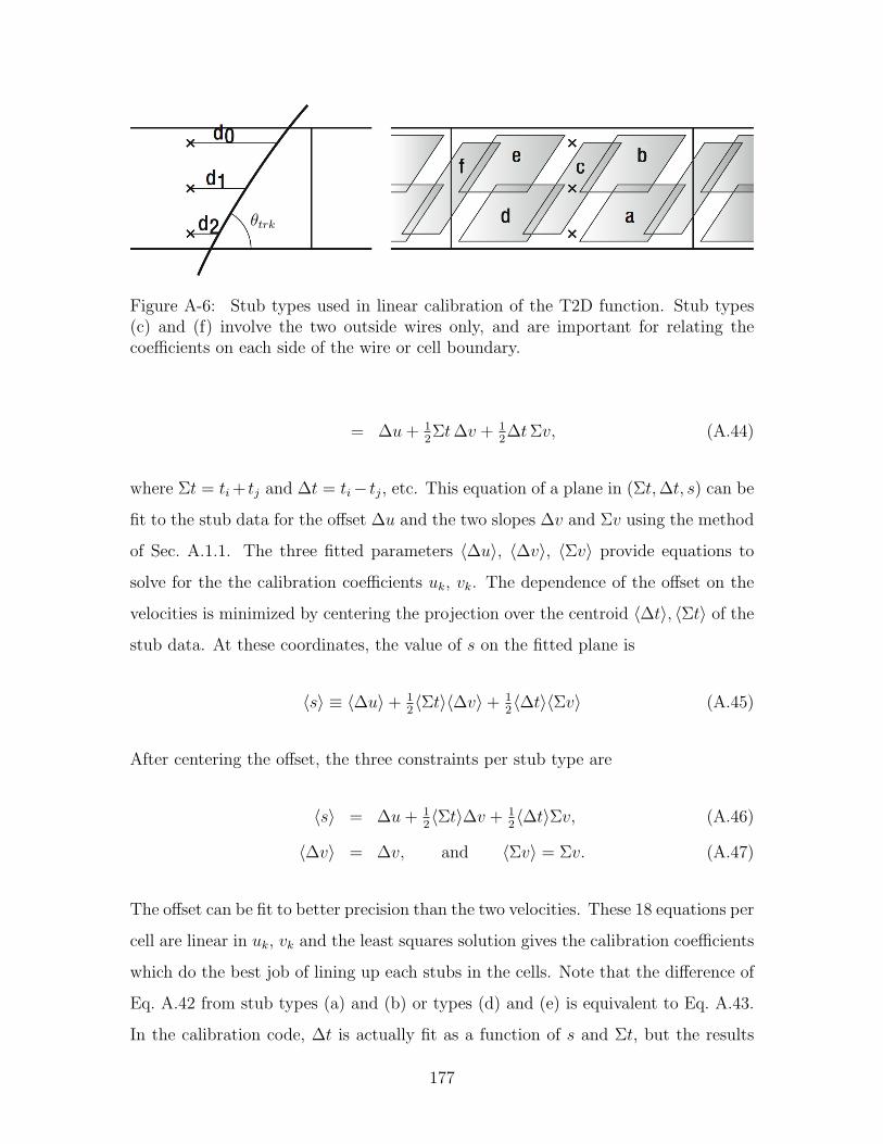
θtrk

Figure A-6: Stub types used in linear calibration of the T2D function. Stub types(c) and (f) involve the two outside wires only, and are important for relating thecoefficients on each side of the wire or cell boundary.

= ∆u + 12Σt ∆v + 1

2∆t Σv, (A.44)

where Σt = ti + tj and ∆t = ti− tj, etc. This equation of a plane in (Σt, ∆t, s) can be

fit to the stub data for the offset ∆u and the two slopes ∆v and Σv using the method

of Sec. A.1.1. The three fitted parameters 〈∆u〉, 〈∆v〉, 〈Σv〉 provide equations to

solve for the the calibration coefficients uk, vk. The dependence of the offset on the

velocities is minimized by centering the projection over the centroid 〈∆t〉, 〈Σt〉 of the

stub data. At these coordinates, the value of s on the fitted plane is

〈s〉 ≡ 〈∆u〉+ 12〈Σt〉〈∆v〉+ 1

2〈∆t〉〈Σv〉 (A.45)

After centering the offset, the three constraints per stub type are

〈s〉 = ∆u + 12〈Σt〉∆v + 1

2〈∆t〉Σv, (A.46)

〈∆v〉 = ∆v, and 〈Σv〉 = Σv. (A.47)

The offset can be fit to better precision than the two velocities. These 18 equations per

cell are linear in uk, vk and the least squares solution gives the calibration coefficients

which do the best job of lining up each stubs in the cells. Note that the difference of

Eq. A.42 from stub types (a) and (b) or types (d) and (e) is equivalent to Eq. A.43.

In the calibration code, ∆t is actually fit as a function of s and Σt, but the results

177

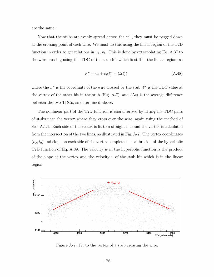
are the same.

Now that the stubs are evenly spread across the cell, they must be pegged down

at the crossing point of each wire. We must do this using the linear region of the T2D

function in order to get relations in uk, vk. This is done by extrapolating Eq. A.37 to

the wire crossing using the TDC of the stub hit which is still in the linear region, as

xwi = ui + vi(t

wj + 〈∆t〉), (A.48)

where the xw is the coordinate of the wire crossed by the stub, tw is the TDC value at

the vertex of the other hit in the stub (Fig. A-7), and 〈∆t〉 is the average difference

between the two TDCs, as determined above.

The nonlinear part of the T2D function is characterized by fitting the TDC pairs

of stubs near the vertex where they cross over the wire, again using the method of

Sec. A.1.1. Each side of the vertex is fit to a straight line and the vertex is calculated

from the intersection of the two lines, as illustrated in Fig. A-7. The vertex coordinates

(tw, t0) and slope on each side of the vertex complete the calibration of the hyperbolic

T2D function of Eq. A.39. The velocity w in the hyperbolic function is the product

of the slope at the vertex and the velocity v of the stub hit which is in the linear

region.

(channels) 0TDC4600 4800 5000 5200 5400 5600

(ch

ann

els)

1T

DC

6100

6200

6300

)0, tw(t

Figure A-7: Fit to the vertex of a stub crossing the wire.

178

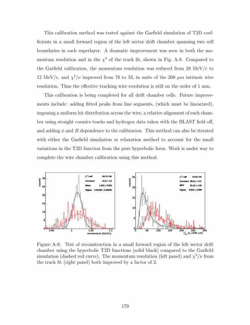
This calibration method was tested against the Garfield simulation of T2D coef-

ficients in a small forward region of the left sector drift chamber spanning two cell

boundaries in each superlayer. A dramatic improvement was seen in both the mo-

mentum resolution and in the χ2 of the track fit, shown in Fig. A-8. Compared to

the Garfield calibration, the momentum resolution was reduced from 28 MeV/c to

12 MeV/c, and χ2/ν improved from 78 to 33, in units of the 200 µm intrinsic wire

resolution. Thus the effective tracking wire resolution is still on the order of 1 mm.

This calibration is being completed for all drift chamber cells. Future improve-

ments include: adding fitted peaks from line segments, (which must be linearized),

imposing a uniform hit distribution across the wire, a relative alignment of each cham-

ber using straight cosmics tracks and hydrogen data taken with the BLAST field off,

and adding φ and B dependence to the calibration. This method can also be iterated

with either the Garfield simulation or relaxation method to account for the small

variations in the T2D function from the pure hyperbolic form. Work is under way to

complete the wire chamber calibration using this method.

/ ndf 2χ 84.74 / 66

Constant 1.9± 21.8

Mean 0.001± 1.015

Sigma 0.00080± 0.01185

momentum (GeV/c) 0.95 1 1.05 1.1

cou

nts

0

5

10

15

20

25

30 / ndf 2χ 84.74 / 66

Constant 1.9± 21.8

Mean 0.001± 1.015

Sigma 0.00080± 0.01185

/ ndf 2χ 72.64 / 84

Constant 7.07± 96.91

MPV 1.06± 33.13

Sigma 0.599± 9.643

m) µ=200 xσ (trk2χ

0 50 100 150 200 250 300

cou

nts

0

5

10

15

20

25 / ndf 2χ 72.64 / 84

Constant 7.07± 96.91

MPV 1.06± 33.13

Sigma 0.599± 9.643

Figure A-8: Test of reconstruction in a small forward region of the left sector driftchamber using the hyperbolic T2D functions (solid black) compared to the Garfieldsimulation (dashed red curve). The momentum resolution (left panel) and χ2/ν fromthe track fit (right panel) both improved by a factor of 2.

179

180

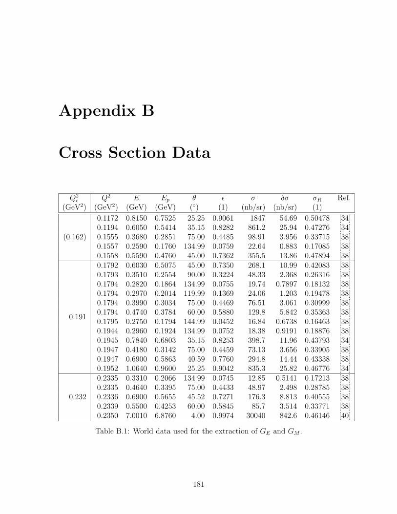
Appendix B

Cross Section Data

Q2c Q2 E Ep θ ε σ δσ σR Ref.

(GeV2) (GeV2) (GeV) (GeV) () (1) (nb/sr) (nb/sr) (1)

(0.162)

0.1172 0.8150 0.7525 25.25 0.9061 1847 54.69 0.50478 [34]0.1194 0.6050 0.5414 35.15 0.8282 861.2 25.94 0.47276 [34]0.1555 0.3680 0.2851 75.00 0.4485 98.91 3.956 0.33715 [38]0.1557 0.2590 0.1760 134.99 0.0759 22.64 0.883 0.17085 [38]0.1558 0.5590 0.4760 45.00 0.7362 355.5 13.86 0.47894 [38]

0.191

0.1792 0.6030 0.5075 45.00 0.7350 268.1 10.99 0.42083 [38]0.1793 0.3510 0.2554 90.00 0.3224 48.33 2.368 0.26316 [38]0.1794 0.2820 0.1864 134.99 0.0755 19.74 0.7897 0.18132 [38]0.1794 0.2970 0.2014 119.99 0.1369 24.06 1.203 0.19478 [38]0.1794 0.3990 0.3034 75.00 0.4469 76.51 3.061 0.30999 [38]0.1794 0.4740 0.3784 60.00 0.5880 129.8 5.842 0.35363 [38]0.1795 0.2750 0.1794 144.99 0.0452 16.84 0.6738 0.16463 [38]0.1944 0.2960 0.1924 134.99 0.0752 18.38 0.9191 0.18876 [38]0.1945 0.7840 0.6803 35.15 0.8253 398.7 11.96 0.43793 [34]0.1947 0.4180 0.3142 75.00 0.4459 73.13 3.656 0.33905 [38]0.1947 0.6900 0.5863 40.59 0.7760 294.8 14.44 0.43338 [38]0.1952 1.0640 0.9600 25.25 0.9042 835.3 25.82 0.46776 [34]

0.232

0.2335 0.3310 0.2066 134.99 0.0745 12.85 0.5141 0.17213 [38]0.2335 0.4640 0.3395 75.00 0.4433 48.97 2.498 0.28785 [38]0.2336 0.6900 0.5655 45.52 0.7271 176.3 8.813 0.40555 [38]0.2339 0.5500 0.4253 60.00 0.5845 85.7 3.514 0.33771 [38]0.2350 7.0010 6.8760 4.00 0.9974 30040 842.6 0.46146 [40]

Table B.1: World data used for the extraction of GE and GM .

181

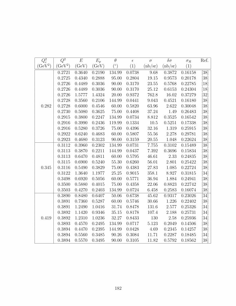
Q2c Q2 E Ep θ ε σ δσ σR Ref.

(GeV2) (GeV2) (GeV) (GeV) () (1) (nb/sr) (nb/sr) (1)

0.282

0.2721 0.3640 0.2190 134.99 0.0738 9.68 0.3872 0.16158 [38]0.2725 0.4340 0.2888 95.00 0.2804 19.15 0.9573 0.20178 [38]0.2726 0.4489 0.3036 90.00 0.3170 23.55 0.5768 0.22785 [18]0.2726 0.4489 0.3036 90.00 0.3170 25.12 0.6153 0.24304 [18]0.2726 1.5777 1.4324 20.00 0.9372 762.8 16.02 0.37279 [32]0.2728 0.3560 0.2106 144.99 0.0441 9.043 0.4521 0.16180 [38]0.2728 0.6000 0.4546 60.00 0.5820 63.96 2.622 0.30048 [38]0.2730 0.5080 0.3625 75.00 0.4408 37.24 1.49 0.26483 [38]0.2915 0.3800 0.2247 134.99 0.0734 8.812 0.3525 0.16542 [38]0.2916 0.3990 0.2436 119.99 0.1334 10.5 0.5251 0.17338 [38]0.2916 0.5280 0.3726 75.00 0.4396 32.16 1.319 0.25915 [38]0.2922 0.6240 0.4683 60.00 0.5807 55.56 2.278 0.29781 [38]0.2923 0.4680 0.3123 90.00 0.3159 20.55 1.048 0.22624 [38]

0.345

0.3112 0.3960 0.2302 134.99 0.0731 7.755 0.3102 0.15489 [38]0.3113 0.3870 0.2211 144.99 0.0437 7.392 0.3696 0.15834 [38]0.3113 0.6470 0.4811 60.00 0.5795 46.61 2.33 0.24835 [38]0.3115 0.6900 0.5240 55.30 0.6260 56.01 2.801 0.25422 [38]0.3116 0.5490 0.3829 75.00 0.4383 27.83 1.085 0.22724 [38]0.3122 1.3640 1.1977 25.25 0.9015 358.1 8.927 0.31815 [34]0.3498 0.6920 0.5056 60.00 0.5771 36.94 1.884 0.24941 [38]0.3500 0.5880 0.4015 75.00 0.4358 22.06 0.8823 0.22742 [38]0.3503 0.4270 0.2403 134.99 0.0724 6.458 0.2583 0.16074 [38]

0.419

0.3890 0.8480 0.6407 50.06 0.6738 45.62 0.9317 0.23026 [34]0.3891 0.7360 0.5287 60.00 0.5746 30.66 1.226 0.22402 [38]0.3891 1.2490 1.0416 31.74 0.8478 131.6 2.577 0.25326 [34]0.3892 1.1420 0.9346 35.15 0.8178 107.4 2.188 0.25731 [34]0.3892 1.2310 1.0236 32.27 0.8433 130 2.58 0.25936 [34]0.3893 0.4570 0.2495 134.99 0.0717 5.123 0.2049 0.14506 [38]0.3894 0.4470 0.2395 144.99 0.0428 4.69 0.2345 0.14257 [38]0.3894 0.5560 0.3485 90.26 0.3084 11.71 0.2287 0.18485 [34]0.3894 0.5570 0.3495 90.00 0.3105 11.82 0.5792 0.18562 [38]

182

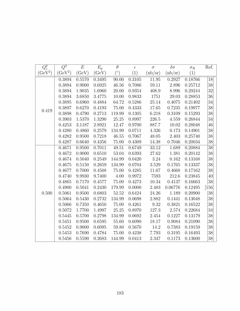
Q2c Q2 E Ep θ ε σ δσ σR Ref.

(GeV2) (GeV2) (GeV) (GeV) () (1) (nb/sr) (nb/sr) (1)

0.419

0.3894 0.5570 0.3495 90.00 0.3105 11.95 0.2927 0.18766 [18]0.3894 0.9000 0.6925 46.56 0.7086 59.11 2.896 0.25712 [38]0.3894 1.9035 1.6960 20.00 0.9354 408.9 8.996 0.29244 [32]0.3894 3.6850 3.4775 10.00 0.9833 1751 29.03 0.28853 [36]0.3895 0.6960 0.4884 64.72 0.5286 25.14 0.4075 0.21402 [34]0.3897 0.6270 0.4193 75.00 0.4333 17.65 0.7235 0.19977 [38]0.3898 0.4790 0.2713 119.99 0.1305 6.218 0.3109 0.15293 [38]0.3903 1.5370 1.3290 25.25 0.8997 226.5 4.559 0.26844 [34]0.4253 3.1187 2.8921 12.47 0.9700 887.7 10.02 0.28048 [46]0.4280 0.4860 0.2579 134.99 0.0711 4.326 0.173 0.14901 [38]0.4282 0.9500 0.7218 46.55 0.7067 48.05 2.403 0.25740 [38]0.4287 0.6640 0.4356 75.00 0.4309 14.38 0.7046 0.20034 [38]

0.500

0.4671 0.9500 0.7011 49.51 0.6749 33.12 1.689 0.20884 [38]0.4672 0.9000 0.6510 53.04 0.6393 27.62 1.381 0.20142 [38]0.4674 0.5040 0.2549 144.99 0.0420 3.24 0.162 0.13168 [38]0.4675 0.5150 0.2659 134.99 0.0704 3.529 0.1765 0.13337 [38]0.4677 0.7000 0.4508 75.00 0.4285 11.67 0.4668 0.17162 [38]0.4740 9.9930 9.7400 4.00 0.9972 7593 212.6 0.23845 [40]0.4865 0.7170 0.4577 75.00 0.4273 10.34 0.4137 0.16663 [38]0.4900 0.5041 0.2430 179.99 0.0000 2.483 0.06776 0.12495 [156]0.5061 0.9500 0.6803 52.52 0.6424 24.26 1.189 0.20900 [38]0.5064 0.5430 0.2732 134.99 0.0698 2.882 0.1441 0.13048 [38]0.5066 0.7350 0.4650 75.00 0.4261 9.32 0.3821 0.16522 [38]0.5072 1.7700 1.4997 25.25 0.8970 127.3 2.574 0.22684 [34]0.5445 0.5700 0.2798 134.99 0.0692 2.454 0.1227 0.13179 [38]0.5451 0.9500 0.6595 55.60 0.6090 18.17 0.9084 0.21090 [38]0.5452 0.9000 0.6095 59.80 0.5670 14.2 0.7383 0.19159 [38]0.5453 0.7690 0.4784 75.00 0.4238 7.793 0.3195 0.16493 [38]0.5456 0.5590 0.2683 144.99 0.0413 2.347 0.1173 0.13600 [38]

183

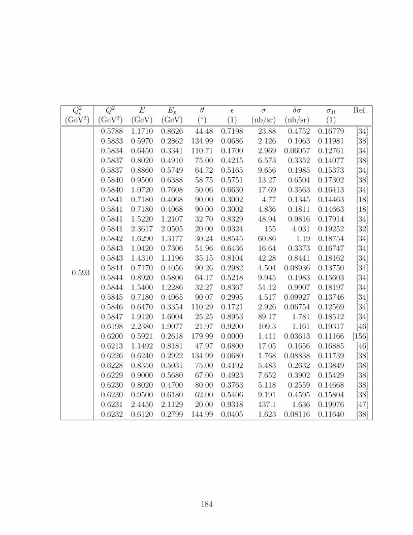
Q2c Q2 E Ep θ ε σ δσ σR Ref.

(GeV2) (GeV2) (GeV) (GeV) () (1) (nb/sr) (nb/sr) (1)

0.593

0.5788 1.1710 0.8626 44.48 0.7198 23.88 0.4752 0.16779 [34]0.5833 0.5970 0.2862 134.99 0.0686 2.126 0.1063 0.11981 [38]0.5834 0.6450 0.3341 110.71 0.1700 2.969 0.06057 0.12761 [34]0.5837 0.8020 0.4910 75.00 0.4215 6.573 0.3352 0.14077 [38]0.5837 0.8860 0.5749 64.72 0.5165 9.656 0.1985 0.15373 [34]0.5840 0.9500 0.6388 58.75 0.5751 13.27 0.6504 0.17302 [38]0.5840 1.0720 0.7608 50.06 0.6630 17.69 0.3563 0.16413 [34]0.5841 0.7180 0.4068 90.00 0.3002 4.77 0.1345 0.14463 [18]0.5841 0.7180 0.4068 90.00 0.3002 4.836 0.1811 0.14663 [18]0.5841 1.5220 1.2107 32.70 0.8329 48.94 0.9816 0.17914 [34]0.5841 2.3617 2.0505 20.00 0.9324 155 4.031 0.19252 [32]0.5842 1.6290 1.3177 30.24 0.8545 60.86 1.19 0.18754 [34]0.5843 1.0420 0.7306 51.96 0.6436 16.64 0.3373 0.16747 [34]0.5843 1.4310 1.1196 35.15 0.8104 42.28 0.8441 0.18162 [34]0.5844 0.7170 0.4056 90.26 0.2982 4.504 0.08936 0.13750 [34]0.5844 0.8920 0.5806 64.17 0.5218 9.945 0.1983 0.15603 [34]0.5844 1.5400 1.2286 32.27 0.8367 51.12 0.9907 0.18197 [34]0.5845 0.7180 0.4065 90.07 0.2995 4.517 0.09927 0.13746 [34]0.5846 0.6470 0.3354 110.29 0.1721 2.926 0.06754 0.12569 [34]0.5847 1.9120 1.6004 25.25 0.8953 89.17 1.781 0.18512 [34]0.6198 2.2380 1.9077 21.97 0.9200 109.3 1.161 0.19317 [46]0.6200 0.5921 0.2618 179.99 0.0000 1.411 0.03613 0.11166 [156]0.6213 1.1492 0.8181 47.97 0.6800 17.05 0.1656 0.16885 [46]0.6226 0.6240 0.2922 134.99 0.0680 1.768 0.08838 0.11739 [38]0.6228 0.8350 0.5031 75.00 0.4192 5.483 0.2632 0.13849 [38]0.6229 0.9000 0.5680 67.00 0.4923 7.652 0.3902 0.15429 [38]0.6230 0.8020 0.4700 80.00 0.3763 5.118 0.2559 0.14668 [38]0.6230 0.9500 0.6180 62.00 0.5406 9.191 0.4595 0.15804 [38]0.6231 2.4450 2.1129 20.00 0.9318 137.1 1.636 0.19976 [47]0.6232 0.6120 0.2799 144.99 0.0405 1.623 0.08116 0.11640 [38]

184

Bibliography

[1] S. Eidelman et al. (Particle Data Group), Phys. Lett. B592, 1 (2004).

[2] V. Punjabi and C. F. Perdrisat, preprint (2005), nucl-ex/0501018, submitted

to PRC, nucl-ex/0501018.

[3] O. Gayou et al. (Jefferson Lab Hall A), Phys. Rev. Lett. 88, 092301 (2002),

nucl-ex/0111010.

[4] A. Afanasev, I. Akushevich, and N. Merenkov, Phys. Rev. D64, 113009 (2001),

hep-ph/0102086.

[5] R. G. Sachs, Phys. Rev. 126, 2256 (1962).

[6] T. W. Donnelly and A. S. Raskin, Annals Phys. 169, 247 (1986).

[7] J. J. Kelly, Phys. Rev. C66, 065203 (2002), hep-ph/0204239.

[8] M. N. Rosenbluth, Phys. Rev. 79, 615 (1950).

[9] N. Dombey, Rev. Mod. Phys. 41, 236 (1969).

[10] A. I. Akhiezer et al., Zhurnal Eksperimental’noi i Teoreticheskoi Fiziki 33, 765

(1957).

[11] R. G. Arnold, C. E. Carlson, and F. Gross, Phys. Rev. C23, 363 (1981).

[12] G. Hohler et al., Nucl. Phys. B114, 505 (1976).

[13] O. Frisch, R.; Stern, Z. Phys. 85, 4 (1933).

185

[14] P. J. Mohr and B. N. Taylor, The 2002 CODATA Recommended Values of the

Fundamental Physical Constants, Tech. rep., National Institute of Standards

and Technology (2004), http://physics.nist.gov/constants.

[15] R. Hofstadter, Rev. Mod. Phys. 28, 214 (1956).

[16] M. Breidenbach et al., Phys. Rev. Lett. 23, 935 (1969).

[17] W. Albrecht et al., Phys. Rev. Lett. 17, 1192 (1966).

[18] L. E. Price et al., Phys. Rev. D4, 45 (1971).

[19] P. N. Kirk et al., Phys. Rev. D8, 63 (1973).

[20] H. Gao, Int. J. Mod. Phys. E12, 1 (2003), nucl-ex/0301002.

[21] L. N. Hand, D. G. Miller, and R. Wilson, Rev. Mod. Phys. 35, 335 (1963).

[22] I. J. J. Murphy, Y. M. Shin, and D. M. Skopik, Phys. Rev. C9, 2444 (1974).

[23] F. Borkowski et al., Nucl. Phys. A222, 269 (1974).

[24] F. Borkowski et al., Nucl. Phys. B93, 461 (1975).

[25] G. G. Simon et al., Nucl. Phys. A333, 381 (1980).

[26] H. Gao and J. Calarco, Precise Determination of the Proton Charge Radius,

Tech. rep., Bates Linear Acelerator Center (2004), experiment E00-02; This ex-

periment was conditionally approved, but not completed before BLAST funding

ended.

[27] P. Mergell, U. G. Meissner, and D. Drechsel, Nucl. Phys. A596, 367 (1996),

hep-ph/9506375.

[28] I. Sick, Phys. Lett. B576, 62 (2003), nucl-ex/0310008.

[29] F. Kottmann, F. Biraben, and C. A. N. C. et al., in G. Cantatore, ed., Quan-

tum Electrodynamics and Physics of the Vacuum, QED 2000 Second Workshop

Proceedings, N. Y. (2001), vol. 564, p. 13.

186

[30] R. C. Walker et al., Phys. Rev. D49, 5671 (1994).

[31] J. Arrington, Phys. Rev. C68, 034325 (2003), nucl-ex/0305009.

[32] M. Goitein et al., Phys. Rev. D1, 2449 (1970).

[33] K. M. Hanson et al., Phys. Rev. D8, 753 (1973).

[34] C. Berger et al., Phys. Lett. B35, 87 (1971).

[35] W. Bartel et al., Nucl. Phys. B58, 429 (1973).

[36] W. Bartel et al., Phys. Rev. Lett. 17, 608 (1966).

[37] W. Albrecht et al., Phys. Rev. Lett. 18, 1014 (1967).

[38] T. Janssens et al., Phys. Rev. 142, 922 (1966).

[39] J. Litt et al., Phys. Lett. B31, 40 (1970).

[40] S. Stein et al., Phys. Rev. D12, 1884 (1975).

[41] S. Rock et al., Phys. Rev. D46, 24 (1992).

[42] P. Bosted et al., Phys. Rev. C42, 38 (1990).

[43] A. F. Sill et al., Phys. Rev. D48, 29 (1993).

[44] L. Andivahis et al., Phys. Rev. D50, 5491 (1994).

[45] D. Dutta et al. (JLab E91013), Phys. Rev. C68, 064603 (2003), nucl-

ex/0303011.

[46] M. E. Christy et al. (E94110), Phys. Rev. C70, 015206 (2004), nucl-ex/0401030.

[47] M. I. Niculescu, Inclusive Resonance Electroproduction Data From Hydrogen

and Deuterium: Studies of Quark Hadron Duality, Ph.D. thesis, Hampton Uni-

versity (1999), experiment E94-110.

[48] I. A. Qattan et al., preprint (2004), nucl-ex/0410010.

187

[49] M. J. Alguard et al., Phys. Rev. Lett. 37, 1258 (1976).

[50] B. D. Milbrath et al. (Bates FPP), Phys. Rev. Lett. 80, 452 (1998), nucl-

ex/9712006.

[51] T. Pospischil et al. (A1), Eur. Phys. J. A12, 125 (2001).

[52] M. K. Jones et al. (Jefferson Lab Hall A), Phys. Rev. Lett. 84, 1398 (2000),

nucl-ex/9910005.

[53] O. Gayou et al., Phys. Rev. C64, 038202 (2001).

[54] D. Eyl et al., Z. Phys. A352, 211 (1995).

[55] S. Dieterich et al., Phys. Lett. B500, 47 (2001), nucl-ex/0011008.

[56] P. E. Bosted, Phys. Rev. C51, 409 (1995).

[57] E. J. Brash et al., Phys. Rev. C65, 051001 (2002), hep-ex/0111038.

[58] J. Arrington, Phys. Rev. C69, 022201 (2004), the world cross sec-

tion data used for fits in this paper are available on the web at

http://www.jlab.org/resdata/resdata protonff.txt, nucl-ex/0309011.

[59] J. J. Kelly, Phys. Rev. C70, 068202 (2004).

[60] J. Friedrich and T. Walcher, Eur. Phys. J. A17, 607 (2003), hep-ph/0303054.

[61] D. R. Yennie, in R. Hofstadter and L. I. Schiff, eds., Nucleon structure; proceed-

ings of the international conference at Stanford University (June 24-27 1963).

[62] L. W. Mo and Y.-S. Tsai, Rev. Mod. Phys. 41, 205 (1969).

[63] L. C. Maximon and J. A. Tjon, Phys. Rev. C62, 054320 (2000), nucl-

th/0002058.

[64] J. Arrington and I. Sick, Phys. Rev. C70, 028203 (2004), nucl-ex/0406014.

188

[65] P. A. M. Guichon and M. Vanderhaeghen, Phys. Rev. Lett. 91, 142303 (2003),

hep-ph/0306007.

[66] J. Arrington, Phys. Rev. C71, 015202 (2005), hep-ph/0408261.

[67] M. P. Rekalo and E. Tomasi-Gustafsson, preprint (2003), nucl-th/0307066.

[68] P. G. Blunden, W. Melnitchouk, and J. A. Tjon, Phys. Rev. Lett. 91, 142304

(2003), nucl-th/0306076.

[69] Y. C. Chen, A. Afanasev, S. J. Brodsky, C. E. Carlson, and M. Vanderhaeghen,

Phys. Rev. Lett. 93, 122301 (2004), hep-ph/0403058.

[70] A. Afanasev et al., in P. S. A. Radyushkin, ed., Exclusive Processes At High

Momentum Transfer: Proceedings (World Scientific, 2002), hep-ph/0208260.

[71] J. Arrington et al., A Measurement of Two-Photon Exchange in Unpolarized

Elastic Electron-Proton Scattering., Tech. rep., TJNAF (2005), experiment Pro-

posal PR-05-017.

[72] R. Gilman et al., Measurement of the Two-Photon Exchange Contribution in

ep Elastic Scattering Using Recoil Polarization, Tech. rep., TJNAF (2004), ex-

periment E-04-019.

[73] J. Arrington, Phys. Rev. C69, 032201 (2004), nucl-ex/0311019.

[74] J. Arrington et al., preprint (2004), nucl-ex/0408020.

[75] A. Afanasev et al., Beyond the Born Approximation: A Precise Comparison of

Positron-Proton and Electron-Proton Elastic Scattering in CLAS, Tech. rep.,

TJNAF (2004), experiment E-04-116.

[76] E. J. Beise, M. L. Pitt, and D. T. Spayde, Prog. Part. Nucl. Phys. 54, 289

(2005), nucl-ex/0412054.

[77] F. E. Maas et al. (A4), Phys. Rev. Lett. 93, 022002 (2004), nucl-ex/0401019.

189

[78] D. Mack et al., Measurements of Target Single-Spin Asymmetry in Elastic ep

Scattering, Tech. rep., TJNAF (2004), experiment Proposal PR-04-008.

[79] D. Mack et al., Measurement of the Born-Forbidden Recoil Proton Normal Po-

larization in Electron-Proton Elastic Scattering, Tech. rep., TJNAF (2004), ex-

periment Proposal PR-04-009.

[80] S. P. Wells et al., Measuring the Two-Photon Exchange Amplitude with Vector

Analyzing Powers in Elastic Electron-Proton Scattering, Tech. rep., TJNAF

(2004), experiment Proposal PR-04-103.

[81] J. Ashman et al. (European Muon), Phys. Lett. B206, 364 (1988).

[82] S. J. Brodsky and G. R. Farrar, Phys. Rev. D11, 1309 (1975).

[83] G. P. Lepage and S. J. Brodsky, Phys. Lett. B87, 359 (1979).

[84] A. V. Belitsky, X.-D. Ji, and F. Yuan, Phys. Rev. D69, 074014 (2004), hep-

ph/0307383.

[85] J. P. Ralston and P. Jain, Phys. Rev. D69, 053008 (2004), hep-ph/0302043.

[86] G. A. Miller, Phys. Rev. C66, 032201 (2002), nucl-th/0207007.

[87] G. A. Miller, in P. S. A. Radyushkin, ed., Exclusive Processes At High Momen-

tum Transfer: Proceedings (World Scientific, 2002), nucl-th/0206027.

[88] F. Cardarelli and S. Simula, Phys. Rev. C62, 065201 (2000), nucl-th/0006023.

[89] M. R. Frank, B. K. Jennings, and G. A. Miller, Phys. Rev. C54, 920 (1996),

nucl-th/9509030.

[90] G. Holzwarth, Z. Phys. A356, 339 (1996), hep-ph/9606336.

[91] R. F. Wagenbrunn, S. Boffi, W. Klink, W. Plessas, and M. Radici, Phys. Lett.

B511, 33 (2001), nucl-th/0010048.

[92] E. L. Lomon, Phys. Rev. C64, 035204 (2001), nucl-th/0104039.

190

[93] O. Gayou, Measurement of the proton form factor ratio µpGEp/GMp up to Q2 =

5.6 GeV2 by recoil polarimetry, PhD dissertation, Universite Blaise Pascal (Apr.

2002).

[94] P. L. Chung and F. Coester, Phys. Rev. D44, 229 (1991).

[95] F. Schlumpf, Phys. Rev. D47, 4114 (1993), hep-ph/9212250.

[96] G. A. Miller and M. R. Frank, Phys. Rev. C65, 065205 (2002), nucl-th/0201021.

[97] P. Kroll, M. Schurmann, and W. Schweiger, Z. Phys. A338, 339 (1991).

[98] B.-Q. Ma, D. Qing, and I. Schmidt, Phys. Rev. C65, 035205 (2002), hep-

ph/0202015.

[99] S. Boffi et al., Eur. Phys. J. A14, 17 (2002), hep-ph/0108271.

[100] W. H. Klink, Phys. Rev. C58, 3587 (1998).

[101] D. H. Lu, S. N. Yang, and A. W. Thomas, Nucl. Phys. A684, 296 (2001).

[102] F. Iachello, A. D. Jackson, and A. Lande, Phys. Lett. B43, 191 (1973).

[103] M. Gari and W. Krumpelmann, Z. Phys. A322, 689 (1985).

[104] M. Gari and W. Krumpelmann, Phys. Lett. B274, 159 (1992).

[105] E. L. Lomon, Phys. Rev. C66, 045501 (2002), nucl-th/0203081.

[106] H. W. Hammer, U.-G. Meissner, and D. Drechsel, Phys. Lett. B385, 343 (1996),

hep-ph/9604294.

[107] B. Kubis and U.-G. Meissner, Nucl. Phys. A679, 698 (2001), hep-ph/0007056.

[108] G. Holzwarth and J. Klomfass, Phys. Rev. D63, 025021 (2001), hep-

ph/0009061.

[109] A. Ali Khan et al. (CP-PACS), Phys. Rev. D65, 054505 (2002), hep-

lat/0105015.

191

[110] A. W. Thomas, Nucl. Phys. Proc. Suppl. 119, 50 (2003), hep-lat/0208023.

[111] M. Gockeler et al. (QCDSF), Phys. Rev. D71, 034508 (2005), hep-lat/0303019.

[112] G. V. Dunne et al., Phys. Lett. B531, 77 (2002), hep-th/0110155.

[113] J. D. Ashley et al., Eur. Phys. J. A19, 9 (2004), hep-lat/0308024.

[114] H. H. Matevosyan, G. A. Miller, and A. W. Thomas, preprint pp. nucl–

th/0501044 (2005), nucl-th/0501044.

[115] R. G. Edwards (Lattice Hadron Physics), Nucl. Phys. Proc. Suppl. 140, 290

(2005), hep-lat/0409119.

[116] D. Beck et al., G0 experiment: Forward Angle Measurements, Tech. rep., TJ-

NAF (2000), experiment E-00-006.

[117] R. Carlini et al., Qweak Experiment: A Search for Physics at the TeV Scale

via a Measurement of the Proton’s Weak Charge, Tech. rep., TJNAF (2000),

experiment E-02-020.

[118] K. A. Aniol et al. (HAPPEX), Phys. Rev. C69, 065501 (2004), nucl-ex/0402004.

[119] X. Zheng et al., Measurements of GpE/Gp

M using elastic ~p(~e, e′p) up to Q2 =

5.6 (GeV/c)2, Tech. rep., TJNAF (2004), experiment Proposal PR-04-111.

[120] M. Farkhondeh et al., in Proceedings of the SPIN-2004 Symposium (2004),

pESP-2004 Workshop.

[121] G. T. Zwart, Polarized electrons at the Bates Accelerator Center South Hall

Ring: Extracted beams and internal targets, Ph.D. thesis, Boston University

(1986).

[122] T. Zwart et al., in Y. I. Makdisi, A. U. Luccio, and W. W. MacKay, eds., 15th

International Spin Physics Symposium (AIP, 2002), vol. 675, p. 1011.

[123] W. Franklin, in Proceedings of the SPIN-2004 Symposium (2004).

192

[124] K. A. Dow, M. Farkhondeh, and J. D. Zumbro, South Hall Ring: Magnetic Mea-

surements of the Lattice Dipoles, Tech. rep., Bates Linear Accelerator Center

(1993).

[125] K. B. Unser, AIP Conf. Proc. 252, 266 (1991).

[126] M. H. Hurwitz, The Compton Polarimeter at Bates, Tech. rep., Bates Linear

Accelerator Center (2003).

[127] W. Franklin et al., in Proceedings of the SPIN-2004 Conference (2004).

[128] V. S. Morozov et al., Phys. Rev. ST Accel. Beams 4, 104002 (2001).

[129] R. V. Cadman et al., Phys. Rev. Lett. 86, 967 (2001).

[130] J. Stenger et al., Phys. Rev. Lett. 78, 4177 (1997).

[131] A. Airapetian et al., Nucl. Instrum. Methods A 540, 68 (2005).

[132] R. V. Cadman, Proton-Deuteron Elastic Scattering and Three-Nucleon Forces,

Ph.D. thesis, University of Illinois at Urbana-Champaign (2001).

[133] V. Ziskin, Measurement of the Electric Form Factor of the Neutron at low

Q2 from a Vector Polarized Deuterium Target at BLAST, Ph.D. thesis, Mas-

sachusetts Institute of Technology (2005).

[134] R. J. Holt et al., in Proceedings of the Eighth International Symposium on High-

Energy Spin Physics, Minneapolis, 1988 (American Institute of Physics, 1989),

p. 1535.

[135] H. Gao, R. J. Holt, et al., in Proc. Int. Wkshp. on Polarized Beams and Polarized

Gas Targets, Cologne, 1995 (World Scientific, 1996), p. 67.

[136] J. Stenger et al., in Proceedings of the International Workshop on polarized

beams and targets, Cologne, 1995 (World Scientific, 1997), p. 85.

[137] C. E. Jones et al., in Proc. Int. Wkshp. on Polarized Beams and Polarized Gas

Targets, Erlangen, 1999 (unpublished, 1999), p. 204.

193

[138] M. A. Miller et al., in Proc. Int. Wkshp. on Polarized Gas Targets and Polarized

Beams, Urbana, 1997 (American Institute of Physics, 1998), p. 148.

[139] C. Crawford et al., in V. Derenchuk and B. von Przewoski, eds., Proc. Int.

Wkshp. on Polarized Sources and Targets, Nashville, Indiana, 2001 (World

Scientific, 2001), p. 78.

[140] B. Clasie et al., Phys. Rev. Lett. (2005), to be submitted.

[141] T. Walker and L. W. Anderson, Nucl. Instrum. Methods. 334, 313 (1993).

[142] J. A. Fedchak et al., Nucl. Instrum. Methods A 391, 405 (1997).

[143] A. Roth, Vacuum Technology (Elsevier Science B. V., 1990).

[144] C. Baumgarten et al., Eur. Phys. J. D 18, 37 (2002).

[145] T. C. Black, Design of a transverse holding-field magnet for the MIT laser-

driven polarized H/D target, Tech. rep., Masachusetts Institute of Technology

(1999).

[146] J. Slevin and W. Stirling, Rev. Sci Instrum. 52, 1780 (1981).

[147] B. Collaboration, Bates Large Acceptance Spectrometer Toroid: Technical De-

sign Report, Tech. rep., Bates Linear Accelerator Center (1997).

[148] A. Goodhue, Analysis of Measurements of the BLAST Magnetic Field, Tech.

rep., Bates Linear Accelerator Center (2002).

[149] B. Zhang, Searching for short range correlations using (e, e′NN) reactions,

Ph.D. thesis, Massachusetts Institute of Technology (2003).

[150] W. H. Press, S. A. Teukolsky, W. T. Vetterling, and B. P. Flannery, Numerical

Recipes in C (Cambridge University Press, 1988).

[151] P. Karpius, Vector Polarization Observables of the Deuteron, Ph.D. thesis, Uni-

versity of New Hampshire (2005).

194

[152] B. Tonguc, in RICH2004 Proceedings; Nucl. Instr. and Methods A (2005).

[153] I. Passchier, The charge form factor of the neutron from double polarized

electron-deuteron scattering, Ph.D. thesis, Vrije Universiteit te Amsterdam

(2000).

[154] T. Ikeda et al., Nucl. Instrum. Meth. A401, 243 (1997).

[155] C. Zhang, Tensor Analyzing Power in Elastic Electron Deuteron Scattering

Below 1 GeV, Ph.D. thesis, Massachusetts Institute of Technology (2006).

[156] P. Bosted et al., Phys. Rev. Lett. 68, 3841 (1992).

195