1

BIRD STRIKE ANALYSIS ON AN AIRCRAFT LEADING EDGE USING

SPH BIRD MODEL

The front facing edges of an airplane, which include the wings, nose cone and

engine, are more prone to bird strikes. In this tutorial, we simulate the bird

strike at the leading edge of an airplane wing structure using smoothed

particles hydrodynamics (SPH) method. The pre-processing of the model is

done in Altair HyperMesh 2017 and is solved in RADIOSS, which is the highly

nonlinear explicit solver of Altair.

Pre-processing of the Model:

1. Launch HyperMesh 2017.

2. Choose User Profile RADIOSS 2017

From File>>Open>>Select file Aircraft_Wing.hm

2

3. Observe the model file loaded. The model has four components which are

the parts of an aircraft wing. The parts are modeled with shell elements.

Creating and Updating Materials:

1. Please notice that the unit system followed for this analysis is Tons,

mm, seconds and Newton.

2. We are using Johnson-Cook Material (/MAT/LAW2) in this model, with

card image M2_PLAS_JOHNS_ZERIL. The material parameters are provided

as shown below.

3

3. Now we will create four different shell properties for the components.

Right click on model browser > Create > Property. The property name is

renamed as skin in the entity editor. Card image is P1_Shell. The thickness

is assigned as 5mm. And also updated with other parameters as shown

below.

4. Similarly for the other three components the above property is duplicated

(right Click skin property, select duplicate and rename) with change in

thickness. That is, for ribs-3mm, spar-1mm, ribs_outer-5mm.

5. The four components are updated with the material created above and

with the respective properties created in the above step.

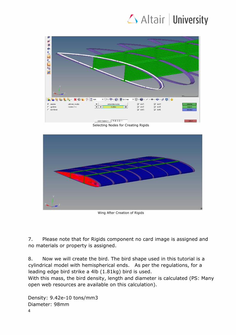
6. Now we are creating a rigid at one side of the aircraft wing, thereby we

are assuming that this end is fixed on to the aircraft fuselage. A new

component collector called Rigids is created. From 1D > Rigids > Create,

now we will create a rigid body. Multiple nodes selection is invoked and the

nodes of the ribs_outer component is selected as shown below and the rigid

is created.

4

Selecting Nodes for Creating Rigids

Wing After Creation of Rigids

7. Please note that for Rigids component no card image is assigned and

no materials or property is assigned.

8. Now we will create the bird. The bird shape used in this tutorial is a

cylindrical model with hemispherical ends. As per the regulations, for a

leading edge bird strike a 4lb (1.81kg) bird is used.

With this mass, the bird density, length and diameter is calculated (PS: Many

open web resources are available on this calculation).

Density: 9.42e-10 tons/mm3

Diameter: 98mm

5

Length: 189mm

Steps for Creating Bird:

1).Create a new component collector for Bird. The bird impact location is

selected and two nodes are created as shown for creating the cylindrical

surface.

2).The cylindrical body is created with the dimensions as below

3).Now two circles are created at the cylinder ends with 49mm radius. After

that, two spheres of 49mm radius are created at the ends of the cylinder as

shown below.

6

4). Now the sphere is trimmed (Geom>Surface edit) with the lines created

therefore hemispherical ends are created for the cylinder. The inner surface

of the sphere is deleted.

5).Now the bird geometry has been created as per the required dimensions.

7

9. With the bird component collector active, go to 1d>SPH.

Select comps from the selector and select the bird component created. The

pitch between particles provided is 5 and enter the density value and click

Create. A property collector, sph_1 is also automatically created now.

10. Now a material is created for the bird. /MAT/LAW6 material law is used

and card image is MLAW6 and the input is provided as below. Assign the

material and sph_1 property to the bird component.

8

11. The loads and boundary conditions for the model are created now.

From Utility Menu, select BCs Manager. Provide a name for the load

collector and select type as Boundary Condition. From the selector choose

nodes and select the master node of the rigid body created. Fix all the

degrees of freedom and click create.

12. From BC’s Manager choose Initial Velocity as the type. Parts selection

is activated and select the Bird component. A velocity of 130000mm/s is

assigned in X-direction. For that, the value is entered in Vx field.

9

13.From Tools> mass calc option, select the Bird component and check the

mass and it shows it is equal to 4lbs, that is 1.8kgs or 1.8 e-3 tons.

14. In the next step we will define contacts between the components.

From Analysis>Interfaces option is selected. The interface is renamed as

Inter_1 and type is selected as Type 7. From the Add option, for master,

components option is selected and ribs, ribs_outer and skin components are

selected as master. For slave, nodes option is selected and the bird particles

are selected as slave and updated. A Gapmin value of 10 is provided and

Inacti is set to 5.

10

15. From Analysis Menu > Output Block is selected, from selector comps is

selected > all the parts are selected > then click Create > Edit. For

NUM_VARIABLES option 1 is given and for Var option DEF is provided. It

means, all default outputs for this part will be provided in the time history

file.

16. Now the engine file is created which contains the run controls. We will

start with run time, /RUN. Right click in Solver browser > Create >Engine

Keywords > RUN. This specifies the run time for this model. We will

provide .005 seconds, that is 5 milliseconds.

A good practice is to create 25 - 30 animation files for the simulation. Here we will

create 25 animation files. For that, right click in Solver browser > Create >Engine

Keywords >ANIM> /ANIM/DT is selected.

11

For frequency of writing time history file TFILE is selected from solver browser and

frequency is given as .00002.

From Solver browser > Create >Engine Keywords >ANIM> ANIM/VERS is selected

and input is given as 44. When the deck includes SPH, one may use

/ANIM/VERS/44.

Output results like energy density, von mises stress, plastic strain..etc. are

requested now. As shown above, right click in Solver browser > Create >Engine

Keywords>ANIM>ANIM/ELEM is selected and required results are checked.

12

17. Now all the required output requests and engine control cards are provided.

The file can now be exported into RADIOSS file type. The model file or deck file

will be saved as xxxx_0000.rad, which is also called as starter file. If the merge

starter and engine file option is not checked a separate file xxxx_0001.rad will also

be created which is the engine file containing the engine controls and output

requests created.

RADIOSS solver is launched and the deck file is uploaded for running the

simulation. Starter out file will be generated (xxxx_0000.out) which gives the

summary of the FE model created (property, materials, parts, contacts, time

step...) and summary of load cases in the form of warnings and/or error messages.

Once the FE model runs fine, the engine file will run according to control card

parameters. The engine file will also create an engine out (xxxx_0001.out) file.

The engine out file gives the cycle summary and termination notification. The user

should continuously monitor the time step in the engine out file. Check for the

abnormal changes in time step.

13

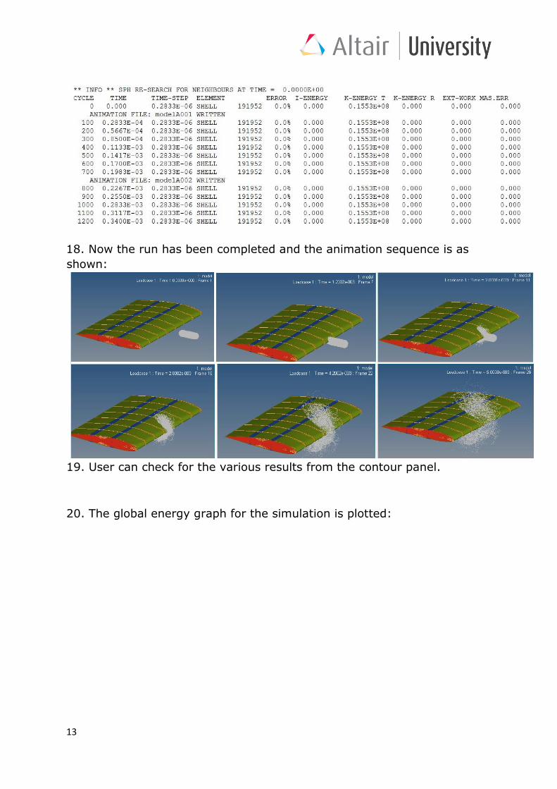
18. Now the run has been completed and the animation sequence is as

shown:

19. User can check for the various results from the contour panel.

20. The global energy graph for the simulation is plotted:

14