Pre-Dredging Sediment Assessment Burford Bank, … Sediment Assessment Burford Bank, Dublin on...
38
Pre-Dredging Sediment Assessment Burford Bank, Dublin on behalf of Dublin Port Moore Marine Services Job No: M07D01 Date: November 2008 Author: Robert Kennedy Client: Jacobs Engineering Atlantic Resource Management Solutions Caherawoneen, Kinvara, Co. Galway
Transcript of Pre-Dredging Sediment Assessment Burford Bank, … Sediment Assessment Burford Bank, Dublin on...

Pre-Dredging Sediment Assessment
Burford Bank, Dublin
on behalf of
Dublin Port
Moore Marine Services
Job No: M07D01
Date: November 2008
Author: Robert Kennedy
Client: Jacobs Engineering
Atlantic Resource Management Solutions Caherawoneen, Kinvara, Co. Galway
TABLE OF CONTENTS
1. INTRODUCTION............................................................................................. 3
1.1 Methods ................................................................................................... 3
1.2 Sediments ................................................................................................. 3
1.3 Macrofauna .............................................................................................. 3
1.4 Sediment Profile Imagery .......................................................................... 6
2. RESULTS........................................................................................................ 6
2.1 Sediments ................................................................................................. 6
2.2 Macrofauna .............................................................................................. 7
2.3 Sediment Profile Imagery .........................................................................17
3. OVERALL ASSESSMENT.................................................................................19
4. LITERATURE CITED .......................................................................................20
TABLE OF FIGURES
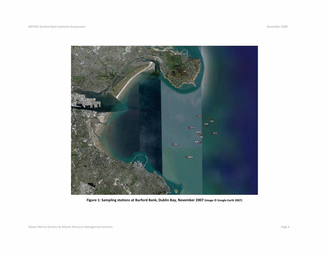
Figure 1: Sampling stations at Burford Bank, Dublin Bay, November 2007 (Image ©
Google Earth 2007)............................................................................................... 4
Figure 2: Principal components analysis (PCA) ordination of sediment data from
Burford Bank, November 2007. Data are standardised and collinear variables have
been removed. See Appendix I. ............................................................................ 7
Figure 3: Multidimensional scaling plot of replicate and mean macrofaunal data
from Burford Bank, November 2007. ...................................................................13

TABLE OF TABLES Table 1a: Results of one way Simper Analyses for species characterizing sites N1 to
N6 at Burford Bank, Dublin Bay, November 2007. ................................................10
Table 1b: Results of one way Simper Analyses for species characterizing sites B1 to
B8 at Burford Bank, Dublin Bay, November
2007……………………………………………………11
Table 2: Results of one-way ANOSIM test for significant differences between
stations. ..............................................................................................................14
Table 3: Results of BioEnv test to link macrofaunal distributions to sediment data.
...........................................................................................................................15
Table 4: Mean and standard deviations of univariate diversity indices from Burford
Bank Grab Fauna, Dublin Bay, November 2007. S=number of species, N= number of
individuals, H’(loge)= Shannon-Wiener diversity index, 1-lambda= Simpson’s index.
For further analysis see Appendix II. ....................................................................16
Table 5: Water Framework Directive Habitat Classification using the Infaunal
Quality Index (IQI). All stations are classified as having high status. .....................17
Table 6: Mean Sediment Profile Imagery results for Burford Bank, Dublin Bay,
November 2007. Penet is the mean prism penetration, aRPD is the mean apparent
redox potential discontinuity, BHQ Stage is the successional stage assigned by the
Benthic Habitat Quality Index, BHQ is the mean BHQ score, OSI is mean Organism
Sediment Index score, WFD BHQ is the Water Framework Directive classification
assigned by BHQ analysis.....................................................................................18

M07D01 Burford Bank Sediment Assessment November 2007
Moore Marine Services & Atlantic Resource Management Systems Page 3
1. Introduction This study was undertaken when Jacobs Engineering commissioned Moore Marine and Atlantic RMS
to carry out a baseline benthic ecological assessment of the dredge spoil disposal site at the Burford
Bank, Dublin Bay. Dublin Port Authority was planning to dredge the maintained navigation channel
into the Port and dispose of the spoil at the Burford Bank. The baseline assessment was carried out
before the dredging operation started. The Burford Bank site had been used in the past by Dublin
Port Authority for similar purposes, and is also used by several other smaller authorities for the ad
hoc disposal of small amounts of spoil material. The purpose of this assessment was to verify that the
site had recovered from previous disposal activities and was fit to receive the current planned spoil
disposal.
1.1 Methods
Sampling was carried out over three days in November 2007. The sample stations are shown in Figure
1. B7 and B8 are control stations that should have had no impact from any previous dumping
activities.
1.2 Sediments
Sediments were sampled at each station using a van Veen grab. Grain size distribution and organic
content were analysed using the methods outlined in Appendix I. The results of these analyses were
used to attempt to explain the distribution of the benthic communities by multivariate analyses, see
Appendix I and below for more details.
1.3 Macrofauna
Benthic macrofauna sample processing
Benthic macrofauna was sampled at each station using a van Veen grab. Five replicate grabs were
taken at each station. Samples were sieved at 1mm, fixed in 4% formaldehyde and later transferred
to 70% alcohol. All fauna was identified to species level where possible. Quality assurance was
provided by the Jacobs benthic lab in the UK who identified 20% of the samples. The remainder was
identified by Atlantic RMS using the most up to date keys available. Species nomenclature was
classified in accordance with Howson & Picton (1997).
Multivariate data analyses
The faunal data matrix was square root transformed and standardised and used to prepare a Bray-
Curtis similarity matrix using Primer 6. The similarity matrix was used to analyse the community
distribution using the following techniques (Clarke & Green 1988; Clarke & Ainsworth 1993; Clarke
1993; Clarke & Warwick 2001):
M07D01 Burford Bank Sediment Assessment November 2008
Moore Marine Services & Atlantic Resource Management Systems Page 4
Figure 1: Sampling stations at Burford Bank, Dublin Bay, November 2007 (Image © Google Earth 2007)

M07D01 Burford Bank Sediment Assessment November 2008
Moore Marine Services & Atlantic Resource Management Systems Page 5
Multi-dimensional scaling (MDS). This is an ordination technique that plots stations in two
dimensions to represent the similarity (usually the Bray Curtis similarity index is used for benthic data)
between stations. Stations that appear close together on the plot are similar to each other (Kruskal &
Wish 1978).
Anosim is an analysis involving permutative Mantel testing to investigate the significance of
differences between stations in similarity matrices. Its output is analogous to that of analysis of
variance. This technique is particularly useful for identifying station groups based on macrofaunal
distributions.
Simper is an exploratory data analysis that is useful for identifying species that characterise station
groups, and also the species that discriminate between groups. It does this by calculating and
comparing the contribution of the component species to within group similarity, and also to between
group dissimilarity. It is particularly useful for biotope classification when combined with ordination of
environmental data by principal components analysis (PCA).
Principal components analysis (PCA) is a standard parametric ordination technique that plots station
distributions in (usually) two dimensions based on linear combinations of variables. It is particularly
suited to analysis of the environmental variables in this study as there are relatively few variables (far
fewer than the likely number of species). Because of potential collinearity in these variables (for
example organic content being high correlated with grain size) some data reduction may be necessary
for this technique
BioEnv is a technique for pattern matching in environmental and biological similarity matrices. In a
similar manner to Anosim, BioEnv uses permutative Mantel testing to find the combination of
environmental variables that best explains the distribution of fauna. It is particularly useful for
explaining the change in biotopes using environmental data. BioEnv was be used to link the faunal
matrices produced in this project to the environmental parameters (Clarke & Ainsworth 1993).
Singular (i.e. unimetric) measures of community structure
The following commonly used summary measures were selected: density (N), species richness (S),
the Shannon–Wiener index (H’) and Simpson’s index. Density is expressed as individuals per
0.1m2
, and species richness as the number of species found at a station. The Shannon–Wiener (H’)
index (Shannon and Weaver, 1949) considers both species richness and the evenness component
of diversity. Simpson’s index is a more explicit measure of the latter, i.e. the proportional
numerical dominance of species in a sample (Simpson, 1949).
Combined (multimetric) univariate measures
For the AMBI index, benthic species are assigned to five ecological groups ranging from sensitive
to highly tolerant of stress. The complementary Biotic Coefficient is calculated according to the
percentage of each ecological group within a sample. Further details are described in Borja et al.
(2000). The index favoured by Ireland and the UK, IQI (Infaunal Quality index), used AMBI,
M07D01 Burford Bank Sediment Assessment November 2008
Moore Marine Services & Atlantic Resource Management Systems Page 6
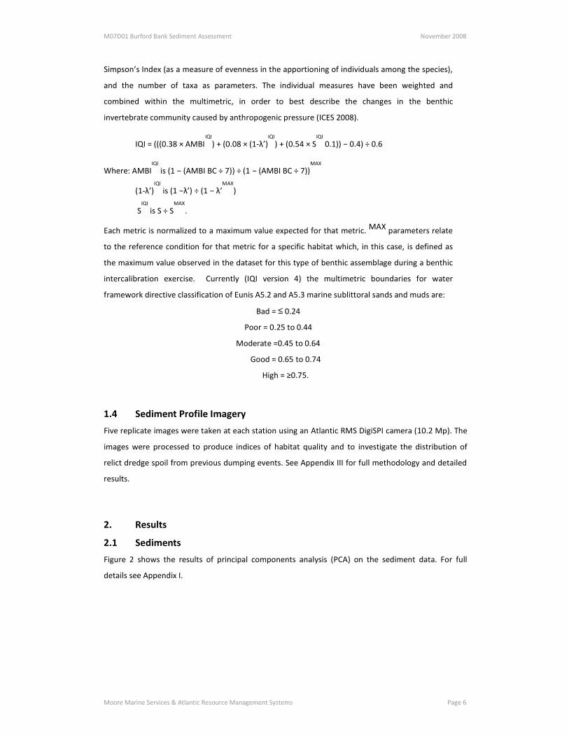
Simpson’s Index (as a measure of evenness in the apportioning of individuals among the species),
and the number of taxa as parameters. The individual measures have been weighted and
combined within the multimetric, in order to best describe the changes in the benthic
invertebrate community caused by anthropogenic pressure (ICES 2008).
IQI = (((0.38 × AMBIIQI
) + (0.08 × (1-λ’)IQI
) + (0.54 × SIQI
0.1)) − 0.4) ÷ 0.6
Where: AMBIIQI
is (1 − (AMBI BC ÷ 7)) ÷ (1 − (AMBI BC ÷ 7))MAX
(1-λ’)IQI
is (1 −λ’) ÷ (1 − λ’MAX
)
SIQI
is S ÷ SMAX
.
Each metric is normalized to a maximum value expected for that metric. MAX parameters relate
to the reference condition for that metric for a specific habitat which, in this case, is defined as
the maximum value observed in the dataset for this type of benthic assemblage during a benthic
intercalibration exercise. Currently (IQI version 4) the multimetric boundaries for water
framework directive classification of Eunis A5.2 and A5.3 marine sublittoral sands and muds are:
Bad = ≤ 0.24
Poor = 0.25 to 0.44
Moderate =0.45 to 0.64
Good = 0.65 to 0.74
High = ≥0.75.
1.4 Sediment Profile Imagery
Five replicate images were taken at each station using an Atlantic RMS DigiSPI camera (10.2 Mp). The
images were processed to produce indices of habitat quality and to investigate the distribution of
relict dredge spoil from previous dumping events. See Appendix III for full methodology and detailed
results.
2. Results
2.1 Sediments
Figure 2 shows the results of principal components analysis (PCA) on the sediment data. For full
details see Appendix I.

M07D01 Burford Bank Sediment Assessment November 2008
Moore Marine Services & Atlantic Resource Management Systems Page 7
Figure 2: Principal components analysis (PCA) ordination of sediment data from Burford Bank, November 2007. Data are standardised and collinear variables have been removed. See Appendix I. In PCA, points that are closer together on the plot are more similar. Linear combinations of the
distributions of the sediment variables were used to create the plot. The equations for PC1 and PC2
are given in Appendix II. The essential message of Figure 2 is that B5, B4, B7 and B8 have relatively
high fine sand and very fine sand content (fs) while N6, N1, N2 and N3 are higher in very coarse sand
(vcs), medium sand (ms) and fine medium sand (fms). B1 is relatively high in silt clay (sc). The raw
sediment data (Appendix I) reveals that all the stations are essentially fine sands with mud. The B
stations tend to be finer that the N stations. All stations have low organic contents (all are <3% by Loss
on Ignition). This PCA ordination accounts for 72.4% of the variation in the sediment data.
2.2 Macrofauna
Simper is an exploratory technique for determining species that characterise communities. Results of
a station by station Simper analysis are shown in Table 1. The N stations are generally characterised
by the polychaetes Nephtys hombergii, Ophelia borealis and Spiophanes bombyx. They conform to the
JNCC habitat SS.SMu.ISaMu.NhomMac Nephtys hombergii and Macoma balthica in infralittoral sandy
mud and with Circalittoral muddy sands SS6 as defined by Fossit (2000). The B stations are generally
characterized by the bivalve Thracia phaseolina, the briitle star Amphiura filiformis and the
polychaete Lagis koreni. These stations correspond with Circalittoral muds SS7 as defined by Fossit

M07D01 Burford Bank Sediment Assessment November 2008
Moore Marine Services & Atlantic Resource Management Systems Page 8
(2000) and the JNCC habitat SS.SMu.CSaMu.AfilMysAnit Amphiura filiformis, Mysella bidentata and
Abra nitida in circalittoral sandy mud. There is generally low similarity between replicates from the
same station, indicating that the sediment type is patchy on small scales or subject to frequent
perturbation.
Figure 3 shows the results of MDS analyses on the replicate and mean faunal data from each station.
The distribution of the faunal communities appears to match their spatial distribution reasonably
well. The stress value (goodness of fit) of the replicate plot is 0.18, indicating that fine scale pattern
may not be well represented. The mean plot has a good stress value at 0.03, and represents the
actual multivariate distribution of the fauna very well. Both ordinations show that B1, B4 and B5 are
similar to B7 and B8. The N samples are less similar to the B samples, N4 being the most similar to the
control sites.
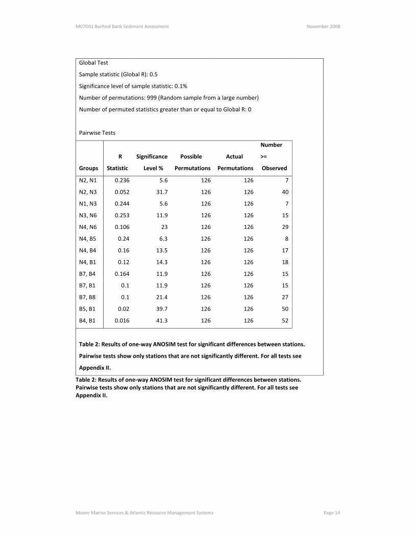
Table 2 shows the results of ANOSIM analysis to determine significant difference between the
communities at the stations. Only stations not significantly different from one another are shown. For
full results see Appendix II. Almost all stations are significantly different from one another. Those that
do show some degree of overlap tend to be the stations closest together, indicating that the
community distribution is reflecting spatially variability, most likely in sediment type. This spatial
variability is probably indicative of physical stress due to shallow water depths, currents, tides and
passing heavy shipping.
Table 3 shows the results of BioEnv analysis to link the macrofaunal and sediment distributions. It
shows that the highest correlation possible (0.802) between the macrofaunal and sediment rank
distance matrices is derived from the distribution of fine medium sand. PCA analysis shows that the N
stations have relatively higher fine medium sand. The next highest possible correlation is 0.742 for
medium sand and fine medium sand, both of which are also associated with the N stations. There is
considerable power in the sediment data to explain the distribution of the macrofauna. The
macrofauna seems to be determined by small scale variation in grain size distribution caused by
physical stress.
Table 4 shows the mean and standard deviations for each univariate diversity index calculated for the
macrofaunal data. The replicate data are shown in Appenix II Table II.2. ANOVA results from analyses
using each diversity index in turn as the response and station as the factor are shown in Appendix II,
Table II.3. There are significant differences between the stations in the case of each diversity index.
Post hoc tests (Tukeys HSD) were performed to determine which stations were significantly different
and which were the same (Appendix II, Table II.4). The results of the post hoc tests indicate that there
are significant differences in terms of number of species (S), number of individuals (N) and Shannon-
Wiener diversity (H’) between N1, N2, N3 and N6 and the reference stations B7 and B8. In the case of
all of these indices the reference stations had a higher mean value indicating better habitat quality.
In general, coarser sediments have less diverse and less populace macrobenthic communitities. We
tested the hypothesis that the lower diversity values were due to differences in grain size distribution
by Spearman’s rank correlation analysis. Results (Table II.5, Appendix II) show that S, N and H’ are

M07D01 Burford Bank Sediment Assessment November 2008
Moore Marine Services & Atlantic Resource Management Systems Page 9
highly significantly correlated with mean grain size, and the lower diversity at these stations may be
due to grain size distribution. This supports the results of the BioEnv analysis.
Table 5 shows the results of the Infaunal Quality Index (IQI) analyses for classifying the habitat quality
of each station for Water Framework Directive (WFD) purposes. All stations were classified as having
high ecological status indicating that the stations had largely recovered from previous dumping
events. IQI is largely based on AMBI. There is some recently published work indicating that,
particularly in shallow coastal water, AMBI may not be very sensitive in detecting disturbance effects
(Zettler et al 2007; Fleischer et al 2007; Ruellet and Dauvin 2007). This may reduce the power of IQI to
detect habitat quality changes, so the results of this analysis should be regarded with a certain degree
of caution. However, the results from this survey are not marginal, and indicate clearly that habitat
quality in the entire area is high.

M07D01 Burford Bank Sediment Assessment November 2008
Moore Marine Services & Atlantic Resource Management Systems Page 10
Group N2 Average similarity: 36.29 Species Av.Abund Av.Sim Sim/SD Contrib% Cum.% Nephtys hombergii 4.43 11.73 0.95 32.32 32.32 Ophelia borealis 4.09 10.82 1.14 29.81 62.13 Group N1 Average similarity: 26.75 Species Av.Abund Av.Sim Sim/SD Contrib% Cum.% Ophelia borealis 4.32 10.44 0.79 39.02 39.02 Nephtys hombergii 3.19 5.83 0.89 21.8 60.82 Group N3 Average similarity: 21.12 Species Av.Abund Av.Sim Sim/SD Contrib% Cum.% Nephtys hombergii 5.26 16.09 1.06 76.2 76.2 Group N4 Average similarity: 23.22 Species Av.Abund Av.Sim Sim/SD Contrib% Cum.% Thracia phaseolina 3.52 7.08 2.29 30.48 30.48 Nephtys hombergii 2.21 4.3 1.11 18.51 48.99 Spiophanes bombyx 2.2 3.12 0.83 13.45 62.44 Group N6 Average similarity: 12.20 Species Av.Abund Av.Sim Sim/SD Contrib% Cum.% Nephtys hombergii 1.62 2.28 0.61 18.69 18.69 NEMERTEA sp. 1.81 2.14 0.57 17.5 36.19 Spiophanes bombyx 1.67 1.71 0.62 14.06 50.25
Table 1a: Results of one way Simper Analyses for species characterizing sites N1 to N6 at Burford Bank, Dublin Bay, November 2007.

M07D01 Burford Bank Sediment Assessment November 2008
Moore Marine Services & Atlantic Resource Management Systems Page 11
Group B7 Average similarity: 36.47 Species Av.Abund Av.Sim Sim/SD Contrib% Cum.% Thracia phaseolina 2.71 4.32 3.23 11.86 11.86 Lagis koreni 2.51 3.27 1.09 8.97 20.82 Amphiura filiformis 2.62 3.08 1.11 8.46 29.28 Melinna palmata 1.79 2.5 2.59 6.84 36.13 Thyasira flexuosa 1.36 2.25 8.37 6.17 42.3 Phaxas pellucidus 1.31 2 2.43 5.49 47.79 Phloe inornata 1.31 1.99 1.15 5.45 53.24 Group B5 Average similarity: 27.31 Species Av.Abund Av.Sim Sim/SD Contrib% Cum.% Sipuncula sp 3.11 5.45 1.08 19.96 19.96 Thracia phaseolina 1.84 2.48 1.08 9.07 29.04 Abra prismatica 1.81 2.37 0.81 8.68 37.72 Spiophanes bombyx 1.87 2.23 1.02 8.17 45.89 Spio decorata 1.57 1.94 1.01 7.12 53.01 Group B4 Average similarity: 39.00 Species Av.Abund Av.Sim Sim/SD Contrib% Cum.% Amphiura filiformis 4.1 8.29 4.79 21.26 21.26 NEMERTEA sp. 2.21 4.07 1.87 10.42 31.68 Thracia phaseolina 2.84 3.6 1.08 9.24 40.92 Nucula nitidosa 1.7 2.88 2.78 7.39 48.31 Ampelisca brevicornis 1.92 2.68 1.12 6.86 55.17 Group B1 Average similarity: 23.63 Species Av.Abund Av.Sim Sim/SD Contrib% Cum.% Sipuncula sp 3.07 4.8 1.12 20.3 20.3 Thracia phaseolina 2.39 2.96 1.07 12.54 32.84 NEMERTEA sp. 1.44 1.68 1.13 7.11 39.94 Amphiura filiformis 1.96 1.5 0.62 6.36 46.31 Lumbrineris gracilis 1.56 1.48 0.82 6.25 52.56 Group B8 Average similarity: 55.78 Species Av.Abund Av.Sim Sim/SD Contrib% Cum.% Amphiura filiformis 4.87 8.71 3.89 15.62 15.62 Thracia phaseolina 3.68 6.42 4.81 11.52 27.14 Lagis koreni 3.36 5.75 3.1 10.3 37.44 Nuculoma tenuis 1.91 3.23 2.24 5.79 43.22 Thyasira flexuosa 1.59 3.04 8.87 5.44 48.66 Abra alba 1.44 2.54 5.79 4.55 53.21
Table 1b: Results of one way Simper Analyses for species characterizing sites B1 to B8 at Burford Bank, Dublin Bay, November 2007.

M07D01 Burford Bank Sediment Assessment November 2008
Moore Marine Services & Atlantic Resource Management Systems Page 12

M07D01 Burford Bank Sediment Assessment November 2008
Moore Marine Services & Atlantic Resource Management Systems Page 13
Figure 3: Multidimensional scaling plot of replicate and mean macrofaunal data from Burford Bank, November 2007.
M07D01 Burford Bank Sediment Assessment November 2008
Moore Marine Services & Atlantic Resource Management Systems Page 14
Global Test
Sample statistic (Global R): 0.5
Significance level of sample statistic: 0.1%
Number of permutations: 999 (Random sample from a large number)
Number of permuted statistics greater than or equal to Global R: 0
Pairwise Tests
R Significance Possible Actual
Number
>=
Groups Statistic Level % Permutations Permutations Observed
N2, N1 0.236 5.6 126 126 7
N2, N3 0.052 31.7 126 126 40
N1, N3 0.244 5.6 126 126 7
N3, N6 0.253 11.9 126 126 15
N4, N6 0.106 23 126 126 29
N4, B5 0.24 6.3 126 126 8
N4, B4 0.16 13.5 126 126 17
N4, B1 0.12 14.3 126 126 18
B7, B4 0.164 11.9 126 126 15
B7, B1 0.1 11.9 126 126 15
B7, B8 0.1 21.4 126 126 27
B5, B1 0.02 39.7 126 126 50
B4, B1 0.016 41.3 126 126 52
Table 2: Results of one-way ANOSIM test for significant differences between stations.
Pairwise tests show only stations that are not significantly different. For all tests see
Appendix II.
Table 2: Results of one-way ANOSIM test for significant differences between stations. Pairwise tests show only stations that are not significantly different. For all tests see Appendix II.

M07D01 Burford Bank Sediment Assessment November 2008
Moore Marine Services & Atlantic Resource Management Systems Page 15
Global Test
Sample statistic (Rho): 0.802
Significance level of sample statistic: 1%
Number of permutations: 99 (Random sample)
Number of permuted statistics greater than or equal to Rho: 0
No.Vars Corr. Selections
1 0.802 5
2 0.746 4,5
3 0.727 4,5,13
2 0.721 5,13
4 0.647 3-5,13
4 0.622 1,4,5,13
2 0.598 3,5
3 0.592 3-5
3 0.591 3,5,13
3 0.579 1,4,5
Variables 1 = vcs, 3 = mcs, 4 = ms, 5 = fms, 6 = fs, 8 = sc, 11 = Skw, 12 = Kur, 13 = OC
Table 3: Results of BioEnv test to link macrofaunal distributions to sediment data.

M07D01 Burford Bank Sediment Assessment November 2008
Moore Marine Services & Atlantic Resource Management Systems Page 16
site S N H'(loge) 1-Lambda' Mean 28 86.8 2.807 0.933 B1 Std. Deviation 13.91 59.701 0.403 0.023 Mean 25 76.2 2.725 0.918 B4 Std. Deviation 10.536 50.366 0.385 0.043 Mean 26.2 62.8 2.837 0.952 B5 Std. Deviation 18.674 59.931 0.536 0.018 Mean 34.4 179.8 2.942 0.924 B7 Std. Deviation 14.223 118.723 0.269 0.019 Mean 36 253.8 2.641 0.868 B8 Std. Deviation 11.937 119.778 0.267 0.047 Mean 8.6 25.8 1.678 0.784 N1 Std. Deviation 5.079 13.971 0.616 0.158 Mean 6.4 21.4 1.537 0.770 N2 Std. Deviation 1.949 10.991 0.407 0.142 Mean 7.4 25.4 1.353 0.662 N3 Std. Deviation 4.506 16.637 0.477 0.188 Mean 22.2 62.6 2.529 0.915 N4 Std. Deviation 14.533 63.752 0.389 0.022 Mean 14.5 33.75 2.231 0.885 N6 Std. Deviation 10.472 30.412 0.738 0.117
Table 4: Mean and standard deviations of univariate diversity indices from Burford Bank Grab Fauna, Dublin Bay, November 2007. S=number of species, N= number of individuals, H’(loge)= Shannon-Wiener diversity index, 1-lambda= Simpson’s index. For further analysis see Appendix II.

M07D01 Burford Bank Sediment Assessment November 2008
Moore Marine Services & Atlantic Resource Management Systems Page 17
Stations AMBI Diversity Richness IQI WFD Class
B1 1.24 5.45 89 0.94 High
B4 1.32 5.05 69 0.91 High
B5 1.25 5.75 86 0.94 High
B7 1.44 5.41 95 0.92 High
B8 1.59 4.38 88 0.90 High
N1 0.71 3.68 27 0.88 High
N2 0.95 2.86 18 0.83 High
N3 0.99 3.53 27 0.86 High
N4 1.15 5.27 82 0.94 High
N6 1.20 4.97 46 0.89 High
Table 5: Water Framework Directive Habitat Classification using the Infaunal Quality Index (IQI). All stations are classified as having high status.
2.3 Sediment Profile Imagery
Functioning as an inverted periscope the sediment profile camera (Rhoads & Cande 1971) slices
vertically through the surficial sediments to take an undisturbed photograph of the sediment profile
(Figure 1). The oxidation state of the surficial sediments and the visible artefacts of bioturbation are
used to calculate indices of benthic habitat quality (Rhoads & Germano 1982, 1986; Nilsson &
Rosenberg 1997), see Appendix III. In this study we also investigated whether there was visible dredge
spoil in the images, and used the system of Rosenberg et al (2004) to classify the sites in terms of
Water framework Directive criteria. Five replicate images were taken at each site, but only good
quality images with sufficient penetration (>4cm) were analysed. Replicate results are shown in
Appendix III, as are representative images from the sites. Summary mean data are shown in Table 6.
Penet
(cm)
aRPD
(cm)
BHQ
Stage BHQ OSI
WFD
BHQ Dredge Spoil
B1 2.7 2.7 2.0 3.0 7.0 poor Oxidised
B4 6.2 4.1 2.0 5.0 9.0 moderate Oxidised
B5 5.9 4.0 2.0 6.0 8.3 moderate Oxidised
B7 4.5 2.8 2.0 6.0 7.3 moderate No
B8 5.4 2.0 2.0 7.0 6.0 Good No
N1 5.1 5.0 1.5 4.5 8.5 moderate No
N2 8.7 5.3 2.0 5.0 9.0 moderate No
N3 3.4 3.4 2.0 3.8 7.6 poor No
N4 7.1 2.1 1.3 2.8 3.8 poor Reduced

M07D01 Burford Bank Sediment Assessment November 2008
Moore Marine Services & Atlantic Resource Management Systems Page 18
N6 4.7 3.4 2.0 5.0 8.0 moderate Oxidised
Table 6: Mean Sediment Profile Imagery results for Burford Bank, Dublin Bay, November 2007. Penet is the mean prism penetration, aRPD is the mean apparent redox potential discontinuity, BHQ Stage is the successional stage assigned by the Benthic Habitat Quality Index, BHQ is the mean BHQ score, OSI is mean Organism Sediment Index score, WFD BHQ is the Water Framework Directive classification assigned by BHQ analysis.
The stations at the edge of the study area, including the control stations, showed no sign of dredge
spoil. B1, B4, B5 and N6 showed signs of spoil from previous dumping, but this spoil was oxidised and
the sites had recovered well. N4 showed signs of both reduced and oxidised dredge spoil. It appeared
that there had been a small amount of recent disposal at the site.
All sites had a well developed mean aRPD (depth of oxidised sediment) at >2.5cm. The WFD
classification was Moderate for most stations, Poor for B1, N3 and N4 and Good for B8. The BHQ is
heavily dependent on seeing animal structures in the sediment profile for awarding good status to
sites. Because these sites are sandier than the fjordic environment where the BHQ was derived,
biogenic structures such as burrows and oxic voids may not as persistent in the sediment profile and
the BHQ may be underestimating habitat quality in this case.
The Organism-Sediment Index of Rhoads & Germano (1982, 1986) is less dependent on observing
particular features in the sediment profile than BHQ. In coastal waters OSI values of less than 6 are
usually taken as being indicative of disturbance. Only N4 is classified as disturbed using this measure.
This is due to the presence of fresh dredge spoil in some of the N4 images.

M07D01 Burford Bank Sediment Assessment November 2008
Moore Marine Services & Atlantic Resource Management Systems Page 19
3. Overall Assessment 1. Sediment analyses reveal that the bottom types are typical of Irish coastal waters, being
muds and muddy fine sand of low organic content. The habitats conform well to those of
Fossitt 2000.
2. The macrobenthic communities are typical of these habitat types and their distribution
appears to be accounted for by changes in grain size distribution in the area using both
multivariate and univariate methods.
3. Habitat quality assessment using the Infaunal Quality Index (IQI) indicated that all of the
stations had high ecological status with reference to water framework directive criteria.
4. Sediment profile Imagery (SPI) analyses revealed that all stations had well oxidized surficial
layers and where dredge spoil was present it was generally well oxidized indicating recovery
from previous dumping events. There was some evidence of recent small scale dumping at
station N4.
5. WFD classification of the SPI data indicated that ecological status was poor to moderate, but
this method of classification is probably over dependent on observing fauna and burrows in
the sediment profile, as it was derived for very cohesive scandanavian fjordic sediments. An
alternative index the OSI indicated that only station N4 was disturbed.
6. Overall, the dumping site appears to have recovered well from previous dredging events and
to be capable of receiving further spoil.
7. The clear mitigation measure necessary is to ensure that any spoil disposed of at the site is
spread evenly around the disposal area, and that no particular area receives too large a
volume of spoil for water currents and macrobenthos to oxidize.

M07D01 Burford Bank Sediment Assessment November 2008
Moore Marine Services & Atlantic Resource Management Systems Page 20
4. Literature cited Clarke, K.R & R.H. Green, 1988. Statistical design and analysis for a biological effects study. Mar. Ecol.
Prog. Ser. 46: 213 - 226.
Clarke, K.R. & M. Ainsworth, 1993. A method of linking multivariate community structure to
environmental variables. Mar. Ecol. Prog. Ser. 92: 205 - 219.
Clarke, K.R. & R.M. Warwick, 2001. Changes in marine communities: an approach to statistical
analysis and interpretation. Natural Environment Research Council, U.K. 2nd Edn.
Clarke, K.R., 1993. Non-parametric multivariate analyses of changes in community structure. Austral.
J. Ecol. 18: 117 - 143.
Connor, D.W, Allen, J.H., Golding, N., Howell, K.L., Lieberknecht, L.M., Northen, K.O., and Reker, J.B.
2004. The Marine Habitat Classification for Britain and Ireland Version 04.05 JNCC, Peterborough.
Fleischer D, Grémare A, Labrune C, Rumohr H, vanden Berghe E and M Zettler 2007. Performance
comparison of two biotic indices measuring the ecological status of water bodies in the Southern
Baltic and Gulf of Lions. Mar. Poll. Bull. 54 (10):1598-1606.
Folk, R.L.,1974. The petrology of sedimentary rocks: Austin, Tx, Hemphill Publishing Co., 182 p.
Fossitt, J. 2000. A Guide to the Habitats of Ireland. The Heritage Council, Ireland. Heiri O, Lotter AF and G Lemcke 2001. Loss on ignition as a method for estimating organic and
carbonate content in sediments: reproducibility and comparability of results. Journal of
Paleolimnology 25: 101–110.
Howson, C M and Picton, B E (eds) 1997. The species directory of the marine fauna and flora of the
British isles and the surrounding sea. Ulster Museum and the Marine Conservation Society, Belfast
and Ross-on-Wye.
ICES. 2008. Report of the Workshop on Benthos Related Environment Metrics (WKBEMET), 11–14 February 2008, Oostende, Belgium. ICES CM 2008/MHC:01. 53 pp.
Kramer, J.M., Brockman, U.H. and Warwick, R.M. 1994. Tidal Estuaries: Manual of Sampling and
Analytical Procedures. A.A. Balkema, Rotterdam, Bookfield.
Kruskal, J.B. & M. Wish, 1978. Multidimensional scaling. Sage Publications, Beverly Hills, California.
Nilsson, H.C. & R. Rosenberg 1997. Benthic habitat quality assessment of an oxygen stressed fjord by
surface and sediment profile images. J. mar. Syst., 11: 249-264.
Pearson, T. H. & R. Rosenberg, 1978. Macrobenthic succession in relation to organic enrichment and
pollution of the marine environment. Oceanogr. mar. Biol. annu. Rev. 16:229-311.
Rhoads, D.C. & J.D. Germano, 1982. Characterisation of organism-sediment relations using sediment
profile imaging: An efficient method of remote ecological monitoring of the seafloor (REMOTS™
system). Mar. Ecol. Prog. Ser. 8: 115 - 128.
Rhoads, D.C. & J.D. Germano, 1986. Interpreting long term changes in benthic community structure: a
new protocol. Hydrobiologia. 142: 291 - 308.

M07D01 Burford Bank Sediment Assessment November 2008
Moore Marine Services & Atlantic Resource Management Systems Page 21
Rhoads, D.C. & S. Cande, 1971. Sediment profile camera for in situ study of organism sediment
relations. Limnol. Oceanogr. 16: 110 - 114.
Ruellet T & Dauvin JC 2007. Benthic indicators: Analysis of the threshold values of ecological quality
classifications for transitional waters. Mar.Poll. Bull. 54(11):1707-1714
Rumohr H 1999. Soft bottom macrofauna: collection, treatment and quality assurance of samples.
ICES Tech Mar Environ Sci 27:1–19
Rosenberg R, Blomqvist M, Nilsson HC, Cederwall H & A Dimming 2004. Marine quality assessment by
use of benthic species-abundance distributions: a proposed new protocol within the European Union
Water Framework Directive. Mar. Poll. Bull. 49: 728-739.
Shannon, C. E., and Weaver, W. 1949. The mathematical theory of communication. University of Illinois Press, Urbana.
Simpson, E. H. 1949. Measurement of diversity. Nature, 163: 688.
Zettler M, Schiedek D, & B Bobertz 2007 Benthic biodiversity indices versus salinity gradient in the
southern Baltic Sea Mar. Poll. Bull. 55 (1-6): 258-270

M07D01 Burford Bank Sediment Assessment November 2008
Moore Marine Services & Atlantic Resource Management Systems Page 22
Appendix I: Sediment analyses and results
Sediment Grain Size Distribution
The particle sizing samples taken from the core slices were frozen (<-20 °C) in zip-lock bags
prior to laser diffraction particle size analysis. Samples were defrosted for 24 hours before analysis to
ensure that no frozen aggregates would distort the particle size distribution frequencies. Samples
were analysed using a Malvern Mastersizer X, capable of sizing in the range of 1-2,000µm. The
samples were sonicated and stirred in distilled water while being analysed. Two replicate runs of
1,000 sweeps of the samples were performed. The distribution of apparent diameters encountered by
the laser in a sample sweep was used to calculate an equivalent sphere diameter particle size
frequency distribution (in which the particles are represented as spheres with the same distribution of
diameters as those measured by the laser). A cumulative frequency plot of the particle size
distributions was constructed from a table of particle size distributions equivalent to a series of
standard sieves.
Sediment descriptive statistics
The 5, 16, 50, 84 and 95 volume percentiles were calculated from the cumulative frequency plots.
These percentiles are used to calculate the following summary statistics developed by Folk (1974) for
the surficial sediment samples.
1) Graphic Mean (Mz)
Mz =(ø16 + ø50 + ø84)
3
where ø = -log2 of particle diameter (mm) of the respective percentiles.
Mz is a measure of the average particle size of the sediment, given in ø units. Negative values
correspond to coarse sand and gravel, while positive values correspond to medium to very fine sands,
clay and silt (see Table I.1).
2) Inclusive graphic standard deviation or Sorting (δi)
δi = ø84 - ø16
4 +
ø95- ø56.6
δi defines the degree of scatter of particle sizes about Mz. A theoretical perfectly
homogeneous sediment would have a δi of 0. Values <1 imply a homogeneous, well sorted sediment,
while those >1 imply a poorly sorted sediment (see Table I.1)
3) Inclusive graphic skewness (Ski)
M07D01 Burford Bank Sediment Assessment November 2008
Moore Marine Services & Atlantic Resource Management Systems Page 23
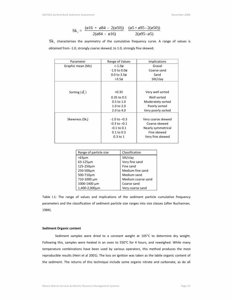
Sk i = (ø16 + ø84 - 2(ø50))
2(ø84 - ø16)+
(ø5 + ø95 - 2(ø50))2(ø95- ø5)
Sk i characterises the asymmetry of the cumulative frequency curve. A range of values is
obtained from -1.0, strongly coarse skewed, to 1.0, strongly fine skewed.
Parameter Range of Values Implications Graphic mean (Mz) <-1.0ø Gravel
-1.0 to 0.0ø Coarse sand 0.0 to 3.5ø Sand >3.5ø Silt/clay
Sorting (δi ) <0.35 Very well sorted
0.35 to 0.5 Well sorted 0.5 to 1.0 Moderately sorted 1.0 to 2.0 Poorly sorted 2.0 to 4.0 Very poorly sorted
Skewness (Ski) -1.0 to –0.3 Very coarse skewed -0.3 to –0.1 Coarse skewed -0.1 to 0.1 Nearly symmetrical 0.1 to 0.3 Fine skewed 0.3 to 1 Very fine skewed
Range of particle size Classification
<63µm Silt/clay 63-125µm Very fine sand 125-250µm Fine sand 250-500µm Medium fine sand 500-710µm 710-1000 µm 1000-1400 µm
Medium sand Medium coarse sand Coarse sand
1,400-2,000µm Very coarse sand
Table I.1: The range of values and implications of the sediment particle cumulative frequency
parameters and the classification of sediment particle size ranges into size classes (after Buchannan,
1984).
Sediment Organic content
Sediment samples were dried to a constant weight at 105°C to determine dry weight.
Following this, samples were heated in an oven to 550°C for 4 hours, and reweighed. While many
temperature combinations have been used by various operators, this method produces the most
reproducible results (Heiri et al 2001). The loss on ignition was taken as the labile organic content of
the sediment. The returns of this technique include some organic nitrate and carbonate, as do all

M07D01 Burford Bank Sediment Assessment November 2008
Moore Marine Services & Atlantic Resource Management Systems Page 24
other standard techniques including chromic acid oxidation (CAOV). For this reason it is better to refer
to this variable as organic content rather than organic carbon. Results are shown in Table I.2.
Sediments principal components analysis
The sediment data were used to make a Pearson’s correlation matrix to check for collinearity
between the sediment variables (Table I.3). Variables that were correlated to other variables in the
data set at 0.8 or above were removed (Mz and cs). The remaining variables were standardised and
normalised, and used in a correlation based principal components analysis to identify the parameters
that account for a large proportion of the variance in the original data set. The variances of the
principal components (Eigen values), the proportion and cumulative proportion of the total variance
explained by each principal component, and the coefficients for each principal component (Eigen
vectors) were calculated. A two-dimensional PCA ordination of the particle size classes and organic
content distributions was made (Figure 2).
(PCA) Principal Component Analysis Eigenvalues PC Eigenvalues %Variation Cum.%Variation 1 4.77 43.4 43.4 2 3.19 29 72.4 Eigenvectors (Coefficients in the linear combinations of variables making up PC's)
Variables PC1 PC2 vcs 0.037 0.308 mcs 0.156 -0.253 ms 0.368 0.101 fms 0.383 0.254 fs -0.358 0.331 vfs -0.44 -0.02 sc -0.044 -0.537 Srt 0.146 0.465 Skw 0.224 -0.336 Kur -0.398 0.151 OC -0.371 -0.127
Table I.3: Principal componenets Analysis (PCA) results for Burford Bank sediments, November 2007. This ordination accounts for 72.4% of the variation in the sediment data. See also Figure 2.

M07D01 Burford Bank Sediment Assessment November 2008
Moore Marine Services & Atlantic Resource Management Systems Page 25
Sample d(v,5) d(v,10) d(v,16) d(v,25) d(v,50) d(v,75) d(v,84) d(v,90) d(v,95) Mz Sort Skew Kurtosis
B4 8.91 11.06 13.95 55.82 178.16 311.28 427.88 570.52 806.64 3.29 -2.22 -0.41 1.07 B1 7.06 7.97 8.76 9.83 12.88 50.35 161.54 826.19 1102.94 5.25 -2.16 0.75 1.27 B5 12.67 38.91 101.57 130.56 190.21 274.75 342.11 446.90 692.01 2.41 -1.31 -0.19 2.20 B7 17.07 97.58 118.01 134.41 166.11 200.59 221.25 244.23 309.12 2.62 -0.86 -0.33 2.96 B8 14.10 86.73 109.67 128.71 163.02 201.46 225.91 255.60 839.72 2.65 -1.15 -0.15 3.74 N1 167.95 195.82 218.72 245.05 313.75 416.18 486.26 578.98 839.05 1.64 -0.64 0.16 1.24 N2 186.82 212.33 236.39 267.87 358.08 504.34 608.83 739.29 1036.50 1.43 -0.72 0.18 1.11 N3 185.56 204.25 221.92 245.97 301.14 374.33 415.71 456.79 512.02 1.72 -0.45 0.04 0.99 N4 32.42 119.24 140.82 162.43 216.05 300.42 364.71 454.69 654.24 2.16 -1.00 -0.08 2.00 N6 120.58 148.39 167.54 189.76 242.01 316.38 366.01 427.71 607.79 2.02 -0.64 0.10 1.30
Sample vcs cs mcs ms fms fs vfs sc LOI%
B4 1.42 1.70 3.42 5.99 20.79 32.24 9.09 25.34 1.54 B1 0.00 7.44 3.44 1.13 1.26 4.99 4.58 77.16 0.78 B5 0.18 1.57 2.99 3.72 21.87 46.69 11.86 11.12 0.69 B7 2.92 1.15 0.33 0.00 4.57 71.70 12.26 7.08 1.55 B8 1.55 2.33 1.74 0.14 5.03 66.36 14.21 8.63 0.97 N1 2.81 1.51 1.89 8.57 58.41 25.03 0.00 1.77 1.69 N2 2.98 2.34 5.69 14.47 54.73 19.78 0.00 0.00 1.47 N3 0.00 0.00 0.06 5.77 67.47 26.69 0.00 0.00 2.48 N4 1.41 0.76 2.08 4.06 28.99 51.29 5.84 5.57 1.81 N6 1.29 1.99 1.29 2.14 39.79 47.91 2.33 3.26 2.08
Table I.2: Sediment grain size and organic content analyses results for Burford Bank sediments, November 2007. d(v,5) is the 5% volume percentile, i.e. 5% of the mass of the sample is smaller than this diameter in microns. Mz is graphic mean, Sort is Sorting, Skew is skewness. vcs is very coarse sand, fs is fine sand etc . See Table I.1 for explanation of these terms. LOI% is the percentage Loss On Ignition and represents the organic content of the sediment.
M07D01 Burford Bank Sediment Assessment November 2008
Moore Marine Services & Atlantic Resource Management Systems Page 26
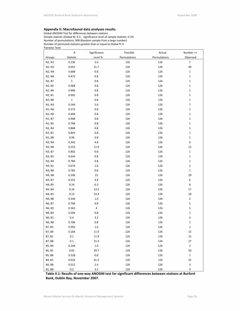
Appendix II: Macrofaunal data analyses results. Global ANOSIM Test for differences between stations Sample statistic (Global R): 0.5; Significance level of sample statistic: 0.1% Number of permutations: 999 (Random sample from a large number) Number of permuted statistics greater than or equal to Global R: 0 Pairwise Tests
R Significance Possible Actual Number >=
Groups Statistic Level % Permutations Permutations Observed
N2, N1 0.236 5.6 126 126 7
N2, N3 0.052 31.7 126 126 40
N2, N4 0.668 0.8 126 126 1
N2, N6 0.475 0.8 126 126 1
N2, B7 1 0.8 126 126 1
N2, B5 0.968 0.8 126 126 1
N2, B4 0.996 0.8 126 126 1
N2, B1 0.992 0.8 126 126 1
N2, B8 1 0.8 126 126 1
N1, N3 0.244 5.6 126 126 7
N1, N4 0.572 0.8 126 126 1
N1, N6 0.469 0.8 126 126 1
N1, B7 0.948 0.8 126 126 1
N1, B5 0.768 0.8 126 126 1
N1, B4 0.868 0.8 126 126 1
N1, B1 0.844 0.8 126 126 1
N1, B8 0.96 0.8 126 126 1
N3, N4 0.342 4.8 126 126 6
N3, N6 0.253 11.9 126 126 15
N3, B7 0.802 0.8 126 126 1
N3, B5 0.634 0.8 126 126 1
N3, B4 0.784 0.8 126 126 1
N3, B1 0.674 1.6 126 126 2
N3, B8 0.782 0.8 126 126 1
N4, N6 0.106 23 126 126 29
N4, B7 0.252 4.8 126 126 6
N4, B5 0.24 6.3 126 126 8
N4, B4 0.16 13.5 126 126 17
N4, B1 0.12 14.3 126 126 18
N4, B8 0.336 1.6 126 126 2
N6, B7 0.706 0.8 126 126 1
N6, B5 0.363 4 126 126 5
N6, B4 0.594 0.8 126 126 1
N6, B1 0.4 3.2 126 126 4
N6, B8 0.706 0.8 126 126 1
B7, B5 0.392 1.6 126 126 2
B7, B4 0.164 11.9 126 126 15
B7, B1 0.1 11.9 126 126 15
B7, B8 0.1 21.4 126 126 27
B5, B4 0.244 1.6 126 126 2
B5, B1 0.02 39.7 126 126 50
B5, B8 0.528 0.8 126 126 1
B4, B1 0.016 41.3 126 126 52
B4, B8 0.312 2.4 126 126 3
B1, B8 0.2 3.2 126 126 4
Table II.1: Results of one-way ANOSIM test for significant differences between stations at Burford Bank, Dublin Bay, November 2007.
M07D01 Burford Bank Sediment Assessment November 2008
Moore Marine Services & Atlantic Resource Management Systems Page 27
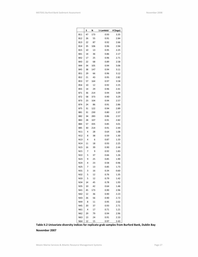
S N 1-Lambda' H'(loge)
B11 47 173 0.93 3.35
B12 26 55 0.91 2.84
B13 22 87 0.92 2.66
B14 35 106 0.96 2.94
B15 10 13 0.95 2.25
B41 14 36 0.86 2.17
B42 17 25 0.96 2.71
B43 22 68 0.89 2.58
B44 34 105 0.94 3.06
B45 38 147 0.94 3.11
B51 29 66 0.96 3.12
B52 21 43 0.95 2.82
B53 57 164 0.97 3.58
B54 10 12 0.92 2.25
B55 14 29 0.96 2.41
B71 36 214 0.94 3.09
B72 58 373 0.90 3.29
B73 23 104 0.94 2.57
B74 24 86 0.91 2.86
B75 31 122 0.94 2.89
B81 31 230 0.80 2.37
B82 34 283 0.86 2.57
B83 28 107 0.91 2.82
B84 57 435 0.85 3.01
B85 30 214 0.91 2.44
N11 4 28 0.64 1.08
N12 8 38 0.59 1.30
N13 4 6 0.87 1.33
N14 11 18 0.93 2.25
N15 16 39 0.90 2.44
N21 7 9 0.92 1.83
N22 5 37 0.66 1.26
N23 9 25 0.85 1.90
N24 4 23 0.58 0.96
N25 7 13 0.85 1.73
N31 3 16 0.34 0.60
N32 5 12 0.76 1.35
N33 5 12 0.79 1.42
N34 14 45 0.78 1.93
N35 10 42 0.64 1.46
N41 45 173 0.90 2.96
N42 12 36 0.90 2.23
N43 26 56 0.90 2.72
N44 8 11 0.95 2.02
N45 20 37 0.93 2.71
N61 4 17 0.71 1.21
N62 29 79 0.94 2.96
N63 13 24 0.91 2.33
N64 12 15 0.97 2.43
Table II.2 Univariate diversity indices for replicate grab samples from Burford Bank, Dublin Bay
November 2007

M07D01 Burford Bank Sediment Assessment November 2008
Moore Marine Services & Atlantic Resource Management Systems Page 28
Sum of Squares df Mean Square F Sig. Between Groups 5418.600 9 602.067 4.376 .001 Within Groups 5365.400 39 137.574
S
Total 10784.000 48 Between Groups 258727.544 9 28747.505 6.446 .000 Within Groups 173941.150 39 4460.029
N
Total 432668.694 48 Between Groups 15.838 9 1.760 8.273 .000 Within Groups 8.296 39 .213
H'(loge)
Total 24.134 48 Between Groups .390 9 .043 4.374 .001 Within Groups .386 39 .010
1-Lambda'
Total .776 48
Table II.3 One way ANOVA results from analyses using Univariate diversity indices as the response
and station as the factor. All results are highly significant.
M07D01 Burford Bank Sediment Assessment November 2008
Moore Marine Services & Atlantic Resource Management Systems Page 29
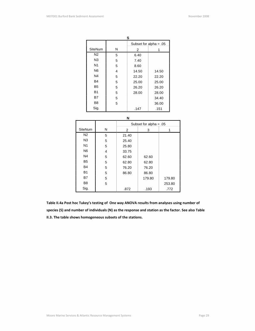
S Subset for alpha = .05
SiteNum N 2 1 N2 5 6.40 N3 5 7.40 N1 5 8.60 N6 4 14.50 14.50 N4 5 22.20 22.20 B4 5 25.00 25.00 B5 5 26.20 26.20 B1 5 28.00 28.00 B7 5 34.40 B8 5 36.00 Sig. .147 .151
N
Subset for alpha = .05 SiteNum N 2 3 1
N2 5 21.40 N3 5 25.40 N1 5 25.80 N6 4 33.75 N4 5 62.60 62.60 B5 5 62.80 62.80 B4 5 76.20 76.20 B1 5 86.80 86.80 B7 5 179.80 179.80 B8 5 253.80 Sig. .872 .193 .772
Table II.4a Post hoc Tukey’s testing of One way ANOVA results from analyses using number of
species (S) and number of individuals (N) as the response and station as the factor. See also Table
II.3. The table shows homogeneous subsets of the stations.

M07D01 Burford Bank Sediment Assessment November 2008
Moore Marine Services & Atlantic Resource Management Systems Page 30
H'(loge)
Subset for alpha = .05 SiteNum N 2 3 1
N3 5 1.35 N2 5 1.54 N1 5 1.68 1.68 N6 4 2.23 2.23 2.23 N4 5 2.53 2.53 B8 5 2.64 2.64 B4 5 2.73 B1 5 2.81 B5 5 2.84 B7 5 2.94 Sig. .121 .062 .349
. 1-Lambda'
Subset for alpha = .05 SiteNum N 2 1
N3 5 .66 N2 5 .77 .77 N1 5 .78 .78 B8 5 .87 .87 N6 4 .88 N4 5 .91 B4 5 .92 B7 5 .92 B1 5 .93 B5 5 .95 Sig. .066 .153
Table II.4b Post hoc Tukey’s testing of One way ANOVA results from analyses using Shannon-
Wiener diversity (H’(loge)) and Simpson’s Index (1-Lambda) as the response and station as the
factor. See also Table II.3. The table shows homogeneous subsets of the stations.

M07D01 Burford Bank Sediment Assessment November 2008
Moore Marine Services & Atlantic Resource Management Systems Page 31
Correlations S N J' H'(loge) 1-Lambda' Mz LOI%
Correlation Coefficient 1.000 .988(**) .248 .855(**) .685(*) .830(**) -.467 Sig. (2-tailed) . .000 .489 .002 .029 .003 .174
S
N 10 10 10 10 10 10 10 Correlation Coefficient .988(**) 1.000 .200 .830(**) .648(*) .879(**) -.455 Sig. (2-tailed) .000 . .580 .003 .043 .001 .187
N
N 10 10 10 10 10 10 10 Correlation Coefficient .855(**) .830(**) .552 1.000 .927(**) .770(**) -.564 Sig. (2-tailed) .002 .003 .098 . .000 .009 .090
H'(loge)
N 10 10 10 10 10 10 10 Correlation Coefficient .685(*) .648(*) .794(**) .927(**) 1.000 .697(*) -.503 Sig. (2-tailed) .029 .043 .006 .000 . .025 .138
1-Lambda'
N 10 10 10 10 10 10 10 Correlation Coefficient .830(**) .879(**) .309 .770(**) .697(*) 1.000 -.503 Sig. (2-tailed) .003 .001 .385 .009 .025 . .138
Mz
N 10 10 10 10 10 10 10 Correlation Coefficient -.467 -.455 -.212 -.564 -.503 -.503 1.000 Sig. (2-tailed) .174 .187 .556 .090 .138 .138 .
Spearman's rho
LOI%
N 10 10 10 10 10 10 10 ** Correlation is significant at the 0.01 level (2-tailed). * Correlation is significant at the 0.05 level (2-tailed).
Table II.5: Spearman’s rank correlation matrix showing the results of correlation analyses between sediment graphic mean (Mz), sediment organic content (LOI%) and
univariate diversity indices. Number of species (S), number of individuals (N) and Shannon Wiener diversity (H’) showed highly significant positive correlation with Mz.,
i.e. the diversity increased as the sediments became finer.
M07D01 Burford Bank Sediment Assessment November 2008
Moore Marine Services & Atlantic Resource Management Systems Page 32
Appendix III: SPI results and representative images
Sediment profile images were captured using an Atlantic RMS DigiSPI digital sediment profile
camera. Images were saved as 10.2 Mpixel 24 bit colour Raw files. Image analysis was performed
using Adobe Photoshop 9.0.2 and Image Analyst 9.0.3 (RVSI Europe Ltd., UK). Image Analyst
interrogates the image at the intensity level, or grey scale value, of individual pixel elements following
a scaling calibration. Grey scale analysis was used to determine the intensity level distribution within
the region of interest and to determine areas of similar grey scale shades. Connectivity analysis was
used to find groups of connected pixels with an intensity value above or below a user-defined
threshold value. Seventeen parameters were either measured or inferred directly from the images in
accordance with standard definitions and methods (Diaz & Schaffer 1988; Solan & Kennedy 2002). The
sediment-water interface was interpolated manually in all images.
The Organism Sediment Index (OSI; Rhoads & Germano 1982, 1986) was calculated using the
method outlined in Table III.2. The successional stage of each image (sensu Rhoads & Germano 1986)
was operator determined by comparing measured and inferred SPI parameters to the ecological
successional paradigm of Pearson & Rosenberg (1978). The Benthic Habitat Quality index (BHQ,
Nilsson & Rosenberg 1997) was calculated as shown in Table III.3. For both indices the lowest index
values are given to those bottoms that lack all surface and subsurface faunal structures and for which
the apparent redox potential discontinuity (aRPD) is either absent or very shallow. The presence of
gas bubbles in the sediment profile or other signs of hypoxia produce the lowest scores in the case of
the OSI. Similarly, the highest index values are assigned to those bottoms that show quantifiable
evidence of extensive infaunal reworking associated with a deep aRPD and the presence of burrows,
feeding voids and visble fauna in the images. The score range can vary from –10 to +11 for the OSI
and from 0 to 15 for the BHQ index.
M07D01 Burford Bank Sediment Assessment November 2008
Moore Marine Services & Atlantic Resource Management Systems Page 33
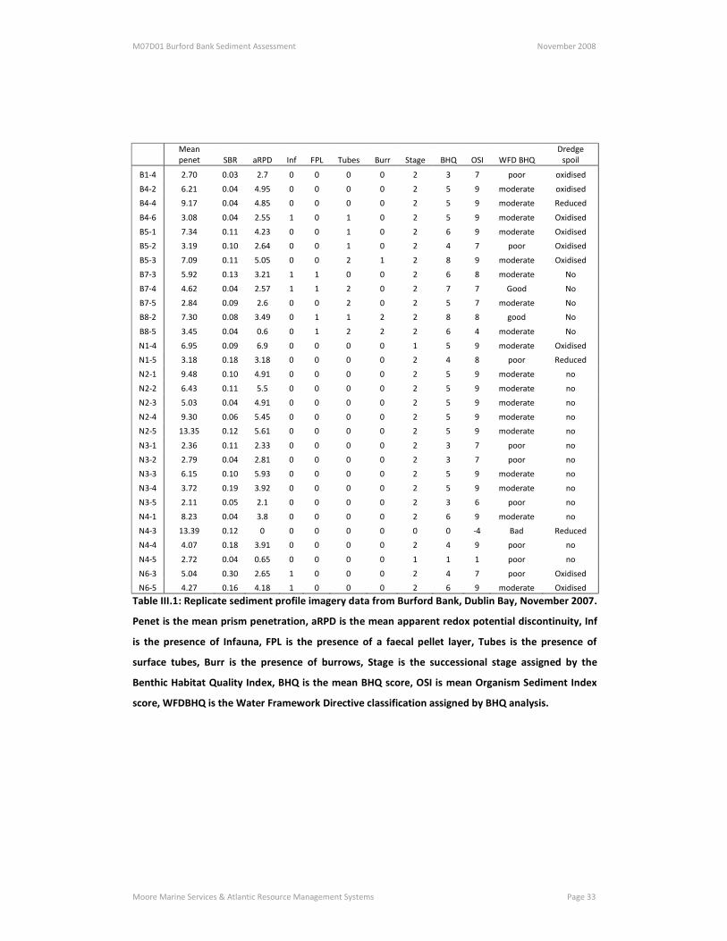
Mean penet SBR aRPD Inf FPL Tubes Burr Stage BHQ OSI WFD BHQ
Dredge spoil
B1-4 2.70 0.03 2.7 0 0 0 0 2 3 7 poor oxidised
B4-2 6.21 0.04 4.95 0 0 0 0 2 5 9 moderate oxidised
B4-4 9.17 0.04 4.85 0 0 0 0 2 5 9 moderate Reduced
B4-6 3.08 0.04 2.55 1 0 1 0 2 5 9 moderate Oxidised
B5-1 7.34 0.11 4.23 0 0 1 0 2 6 9 moderate Oxidised
B5-2 3.19 0.10 2.64 0 0 1 0 2 4 7 poor Oxidised
B5-3 7.09 0.11 5.05 0 0 2 1 2 8 9 moderate Oxidised
B7-3 5.92 0.13 3.21 1 1 0 0 2 6 8 moderate No
B7-4 4.62 0.04 2.57 1 1 2 0 2 7 7 Good No
B7-5 2.84 0.09 2.6 0 0 2 0 2 5 7 moderate No
B8-2 7.30 0.08 3.49 0 1 1 2 2 8 8 good No
B8-5 3.45 0.04 0.6 0 1 2 2 2 6 4 moderate No
N1-4 6.95 0.09 6.9 0 0 0 0 1 5 9 moderate Oxidised
N1-5 3.18 0.18 3.18 0 0 0 0 2 4 8 poor Reduced
N2-1 9.48 0.10 4.91 0 0 0 0 2 5 9 moderate no
N2-2 6.43 0.11 5.5 0 0 0 0 2 5 9 moderate no
N2-3 5.03 0.04 4.91 0 0 0 0 2 5 9 moderate no
N2-4 9.30 0.06 5.45 0 0 0 0 2 5 9 moderate no
N2-5 13.35 0.12 5.61 0 0 0 0 2 5 9 moderate no
N3-1 2.36 0.11 2.33 0 0 0 0 2 3 7 poor no
N3-2 2.79 0.04 2.81 0 0 0 0 2 3 7 poor no
N3-3 6.15 0.10 5.93 0 0 0 0 2 5 9 moderate no
N3-4 3.72 0.19 3.92 0 0 0 0 2 5 9 moderate no
N3-5 2.11 0.05 2.1 0 0 0 0 2 3 6 poor no
N4-1 8.23 0.04 3.8 0 0 0 0 2 6 9 moderate no
N4-3 13.39 0.12 0 0 0 0 0 0 0 -4 Bad Reduced
N4-4 4.07 0.18 3.91 0 0 0 0 2 4 9 poor no
N4-5 2.72 0.04 0.65 0 0 0 0 1 1 1 poor no
N6-3 5.04 0.30 2.65 1 0 0 0 2 4 7 poor Oxidised
N6-5 4.27 0.16 4.18 1 0 0 0 2 6 9 moderate Oxidised
Table III.1: Replicate sediment profile imagery data from Burford Bank, Dublin Bay, November 2007.
Penet is the mean prism penetration, aRPD is the mean apparent redox potential discontinuity, Inf
is the presence of Infauna, FPL is the presence of a faecal pellet layer, Tubes is the presence of
surface tubes, Burr is the presence of burrows, Stage is the successional stage assigned by the
Benthic Habitat Quality Index, BHQ is the mean BHQ score, OSI is mean Organism Sediment Index
score, WFDBHQ is the Water Framework Directive classification assigned by BHQ analysis.
M07D01 Burford Bank Sediment Assessment November 2008
Moore Marine Services & Atlantic Resource Management Systems Page 34
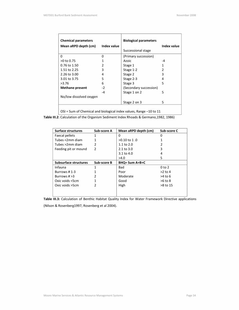
Chemical parameters Biological parameters
Mean aRPD depth (cm) Index value Successional stage
Index value
0 0 (Primary succession) >0 to 0.75 1 Azoic -4 0.76 to 1.50 2 Stage 1 1 1.51 to 2.25 3 Stage 1-2 2 2.26 to 3.00 4 Stage 2 3 3.01 to 3.75 5 Stage 2-3 4 >3.76 6 Stage 3 5 Methane present -2 (Secondary succession)
No/low dissolved oxygen -4 Stage 1 on 2 5
Stage 2 on 3 5
OSI = Sum of Chemical and biological index values, Range –10 to 11
Table III.2: Calculation of the Organism Sediment Index Rhoads & Germano,1982, 1986)
Surface structures Sub-score A Mean aRPD depth (cm) Sub-score C Faecal pellets 1 0 0 Tubes <2mm diam 1 >0.10 to 1 .0 1 Tubes >2mm diam 2 1.1 to 2.0 2 Feeding pit or mound 2 2.1 to 3.0 3 3.1 to 4.0 4 >4.0 5 Subsurface structures Sub-score B BHQ= Sum A+B+C Infauna 1 Bad 0 to 2 Burrows # 1-3 1 Poor >2 to 4 Burrows # >3 2 Moderate >4 to 6 Oxic voids <5cm Oxic voids >5cm
1 2
Good High
>6 to 8 >8 to 15
Table III.3: Calculation of Benthic Habitat Quality Index for Water Framework Directive applications
(Nilson & Rosenberg1997, Rosenberg et al 2004).

M07D01 Burford Bank Sediment Assessment November 2008
Moore Marine Services & Atlantic Resource Management Systems Page 35
Representative Images Dublin Bay, November 2007.
N1 N2 N3
§ Clean sand, no trace of dredge spoil
B5 N6
• Oxidised fine sediments underlying dredge spoil. These sediments are recovering well from
previous disposal events.
• There is extensive recolonisation by benthic animals

M07D01 Burford Bank Sediment Assessment November 2008
Moore Marine Services & Atlantic Resource Management Systems Page 36
N4 N4
• Very variable station
• Images taken within 2 minutes of each other
• The image on the left shows recent spoil disposal, perhaps on a small scale?
• The image on right is more typical of the station
B1 B4
• Hard ground with spoil overlying fine sand and clay. Large burrowing worm visible in B4
image.
• These stations have recovered following previous disposal events.
M07D01 Burford Bank Sediment Assessment November 2008
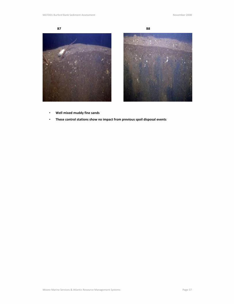
Moore Marine Services & Atlantic Resource Management Systems Page 37
B7 B8
• Well mixed muddy fine sands
• These control stations show no impact from previous spoil disposal events