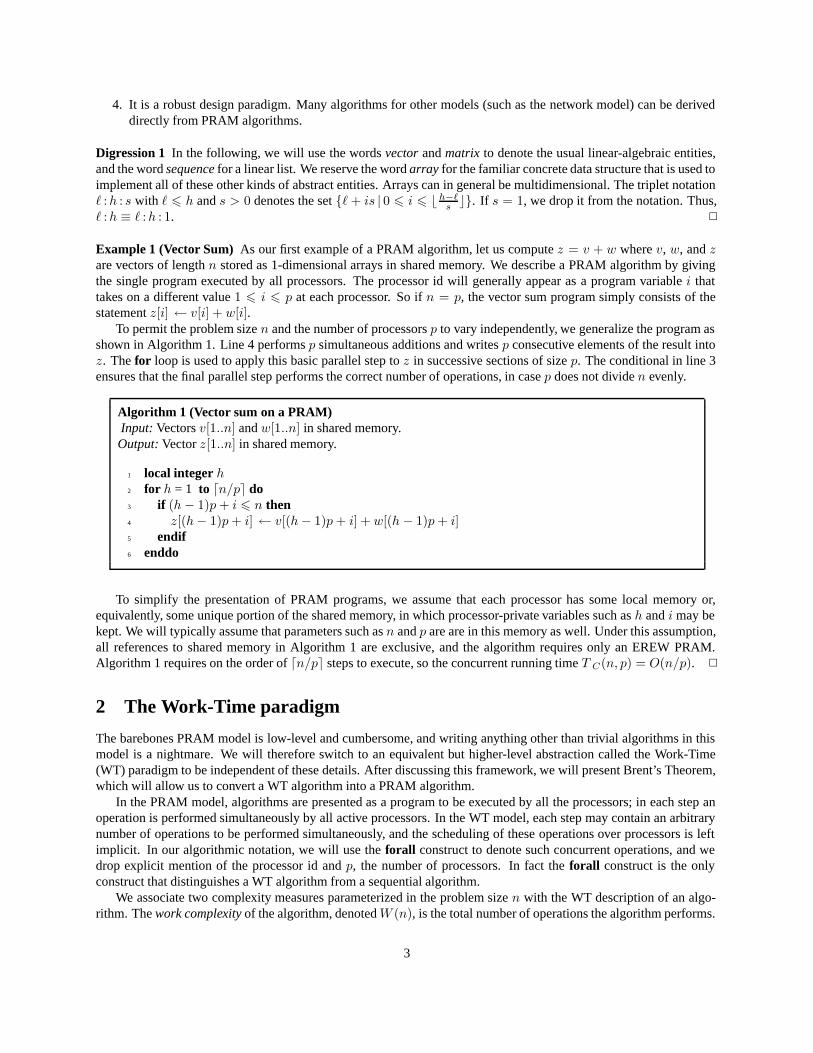
COMP 633: Parallel ComputingPRAM Algorithms

Siddhartha ChatterjeeJan Prins

Fall 2009c© Siddhartha Chatterjee, Jan Prins 2009

Contents

1 The PRAM model of computation 1

2 The Work-Time paradigm 32.1 Brent’s Theorem . . . . . . . . . . . . . . . . . . . . . . . . . . . . . . . . . . . . . . . . . . . . . 52.2 Designing good parallel algorithms . . . . . . . . . . . . . . . . . . . . . . . . . . . . . . . . . . . . 6

3 Basic PRAM algorithm design techniques 73.1 Balanced trees . . . . . . . . . . . . . . . . . . . . . . . . . . . . . . . . . . . . . . . . . . . . . . . 73.2 Pointer jumping . . . . . . . . . . . . . . . . . . . . . . . . . . . . . . . . . . . . . . . . . . . . . . 93.3 Algorithm cascading . . . . . . . . . . . . . . . . . . . . . . . . . . . . . . . . . . . . . . . . . . . 113.4 Euler tours . . . . . . . . . . . . . . . . . . . . . . . . . . . . . . . . . . . . . . . . . . . . . . . . . 123.5 Divide and conquer . . . . . . . . . . . . . . . . . . . . . . . . . . . . . . . . . . . . . . . . . . . . 143.6 Symmetry breaking . . . . . . . . . . . . . . . . . . . . . . . . . . . . . . . . . . . . . . . . . . . . 16

4 A tour of data-parallel algorithms 184.1 Basic scan-based algorithms . . . . . . . . . . . . . . . . . . . . . . . . . . . . . . . . . . . . . . . 184.2 Parallel lexical analysis . . . . . . . . . . . . . . . . . . . . . . . . . . . . . . . . . . . . . . . . . . 20

5 The relative power of PRAM models 215.1 The power of concurrent reads . . . . . . . . . . . . . . . . . . . . . . . . . . . . . . . . . . . . . . 215.2 The power of concurrent writes . . . . . . . . . . . . . . . . . . . . . . . . . . . . . . . . . . . . . . 215.3 Quantifying the power of concurrent memory accesses . . . . . . . . . . . . . . . . . . . . . . . . . 225.4 Relating the PRAM model to practical parallel computation . . . . . . . . . . . . . . . . . . . . . . . 23

1 The PRAM model of computation

In the first unit of the course, we will study parallel algorithms in the context of a model of parallel computation calledthe Parallel Random Access Machine (PRAM). As the name suggests, the PRAM model is an extension of the familiarRAM model of sequential computation that is used in algorithm analysis. We will use the synchronous PRAM whichis defined as follows.

1. There are p processors connected to a single shared memory.

2. Each processor has a unique index 1 � i � p called the processor id.

3. A single program is executed in single-instruction stream, multiple-data stream (SIMD) fashion. Each instruc-tion in the instruction stream is carried out by all processors simultaneously and requires unit time, regardlessof the number of processors.

4. Each processor has a flag that controls whether it is active in the execution of an instruction. Inactive processorsdo not participate in the execution of instructions, except for instructions that reset the flag.

The processor id can be used to distinguish processor behavior while executing the common program. For example,each processor can use its processor id to form a distinct address in the shared memory from which to read a value.A sequence of instructions can be conditionally executed by a subset of processors. The condition is evaluated by allprocessors and is used to set the processor active flags. Only active processors carry out the instructions that follow.At the end of the sequence the flags are reset so that execution is resumed by all processors.

The operation of a synchronous PRAM can result in simultaneous access by multiple processors to the samelocation in shared memory. There are several variants of our PRAM model, depending on whether such simultaneousaccess is permitted (concurrent access) or prohibited (exclusive access). As accesses can be reads or writes, we havethe following four possibilities:

1. Exclusive Read Exclusive Write (EREW): This PRAM variant does not allow any kind of simultaneous accessto a single memory location. All correct programs for such a PRAM must insure that no two processors accessa common memory location in the same time unit.

2. Concurrent Read Exclusive Write (CREW): This PRAM variant allows concurrent reads but not concurrentwrites to shared memory locations. All processors concurrently reading a common memory location obtain thesame value.

3. Exclusive Read Concurrent Write (ERCW): This PRAM variant allows concurrent writes but not concurrentreads to shared memory locations. This variant is generally not considered independently, but is subsumedwithin the next variant.

4. Concurrent Read Concurrent Write (CRCW): This PRAM variant allows both concurrent reads and concur-rent writes to shared memory locations. There are several sub-variants within this variant, depending on howconcurrent writes are resolved.

(a) Common CRCW: This model allows concurrent writes if and only if all the processors are attempting towrite the same value (which becomes the value stored).

(b) Arbitrary CRCW: In this model, a value arbitrarily chosen from the values written to the common mem-ory location is stored.

(c) Priority CRCW: In this model, the value written by the processor with the minimum processor id writingto the common memory location is stored.

(d) Combining CRCW: In this model, the value stored is a combination (usually by an associative and com-mutative operator such as + or max) of the values written.

The different models represent different constraints in algorithm design. They differ not in expressive power butin complexity-theoretic terms. We will consider this issue further in Section 5.

We study PRAM algorithms for several reasons.

1. There is a well-developed body of literature on the design of PRAM algorithms and the complexity of suchalgorithms.

2. The PRAM model focuses exclusively on concurrency issues and explicitly ignores issues of synchronizationand communication. It thus serves as a baseline model of concurrency. In other words, if you can’t get a goodparallel algorithm on the PRAM model, you’re not going to get a good parallel algorithm in the real world.

3. The model is explicit: we have to specify the operations performed at each step, and the scheduling of operationson processors.

2

4. It is a robust design paradigm. Many algorithms for other models (such as the network model) can be deriveddirectly from PRAM algorithms.

Digression 1 In the following, we will use the words vector and matrix to denote the usual linear-algebraic entities,and the word sequence for a linear list. We reserve the word array for the familiar concrete data structure that is used toimplement all of these other kinds of abstract entities. Arrays can in general be multidimensional. The triplet notation� :h : s with � � h and s > 0 denotes the set {�+ is | 0 � i � � h−�

s �}. If s = 1, we drop it from the notation. Thus,� :h ≡ � :h : 1. �

Example 1 (Vector Sum) As our first example of a PRAM algorithm, let us compute z = v + w where v, w, and zare vectors of length n stored as 1-dimensional arrays in shared memory. We describe a PRAM algorithm by givingthe single program executed by all processors. The processor id will generally appear as a program variable i thattakes on a different value 1 � i � p at each processor. So if n = p, the vector sum program simply consists of thestatement z[i] ← v[i] + w[i].

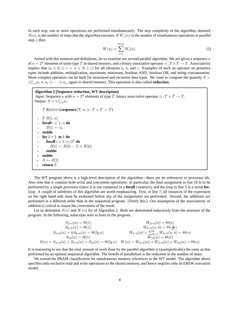
To permit the problem size n and the number of processors p to vary independently, we generalize the program asshown in Algorithm 1. Line 4 performs p simultaneous additions and writes p consecutive elements of the result intoz. The for loop is used to apply this basic parallel step to z in successive sections of size p. The conditional in line 3ensures that the final parallel step performs the correct number of operations, in case p does not divide n evenly.

Algorithm 1 (Vector sum on a PRAM)Input: Vectors v[1..n] and w[1..n] in shared memory.Output: Vector z[1..n] in shared memory.

1 local integer h2 for h = 1 to �n/p� do3 if (h− 1)p+ i � n then4 z[(h− 1)p+ i] ← v[(h− 1)p+ i] + w[(h− 1)p+ i]5 endif6 enddo

To simplify the presentation of PRAM programs, we assume that each processor has some local memory or,equivalently, some unique portion of the shared memory, in which processor-private variables such as h and i may bekept. We will typically assume that parameters such as n and p are are in this memory as well. Under this assumption,all references to shared memory in Algorithm 1 are exclusive, and the algorithm requires only an EREW PRAM.Algorithm 1 requires on the order of �n/p� steps to execute, so the concurrent running time T C(n, p) = O(n/p). �

2 The Work-Time paradigm

The barebones PRAM model is low-level and cumbersome, and writing anything other than trivial algorithms in thismodel is a nightmare. We will therefore switch to an equivalent but higher-level abstraction called the Work-Time(WT) paradigm to be independent of these details. After discussing this framework, we will present Brent’s Theorem,which will allow us to convert a WT algorithm into a PRAM algorithm.

In the PRAM model, algorithms are presented as a program to be executed by all the processors; in each step anoperation is performed simultaneously by all active processors. In the WT model, each step may contain an arbitrarynumber of operations to be performed simultaneously, and the scheduling of these operations over processors is leftimplicit. In our algorithmic notation, we will use the forall construct to denote such concurrent operations, and wedrop explicit mention of the processor id and p, the number of processors. In fact the forall construct is the onlyconstruct that distinguishes a WT algorithm from a sequential algorithm.

We associate two complexity measures parameterized in the problem size n with the WT description of an algo-rithm. The work complexity of the algorithm, denotedW (n), is the total number of operations the algorithm performs.

3

In each step, one or more operations are performed simultaneously. The step complexity of the algorithm, denotedS(n), is the number of steps that the algorithm executes. IfW i(n) is the number of simultaneous operations at parallelstep i, then

W (n) =S(n)∑i=1

Wi(n). (1)

Armed with this notation and definitions, let us examine our second parallel algorithm. We are given a sequence aof n = 2k elements of some type T in shared memory, and a binary associative operator⊕ :T ×T → T . Associativityimplies that (a ⊕ b) ⊕ c = a ⊕ (b ⊕ c) for all elements a, b, and c. Examples of such an operator on primitivetypes include addition, multiplication, maximum, minimum, boolean AND, boolean OR, and string concatenation.More complex operators can be built for structured and recursive data types. We want to compute the quantity S =⊕n

i=1ai ≡ a1 ⊕ · · · ⊕ an, again in shared memory. This operation is also called reduction.

Algorithm 2 (Sequence reduction, WT description)Input: Sequence a with n = 2k elements of type T , binary associative operator⊕ :T × T → T .Output: S = ⊕n

i=1ai.

T REDUCE(sequence〈T〉 a, ⊕ :T × T → T )

1 T B[1..n]2 forall i ∈ 1 :n do3 B[i] ← ai

4 enddo5 for h = 1 to k do6 forall i ∈ 1 :n/2h do7 B[i] ← B[2i− 1]⊕B[2i]8 enddo9 enddo

10 S ← B[1]11 return S

The WT program above is a high-level description of the algorithm—there are no references to processor ids.Also note that it contains both serial and concurrent operations. In particular, the final assignment in line 10 is to beperformed by a single processor (since it is not contained in a forall construct), and the loop in line 5 is a serial for-loop. A couple of subtleties of this algorithm are worth emphasizing. First, in line 7, all instances of the expressionon the right hand side must be evaluated before any of the assignments are performed. Second, the additions areperformed in a different order than in the sequential program. (Verify this.) Our assumption of the associativity ofaddition is critical to insure the correctness of the result.

Let us determine S(n) and W (n) for of Algorithm 2. Both are determined inductively from the structure of theprogram. In the following, subscripts refer to lines in the program.

S2–4(n) = Θ(1) W2–4(n) = Θ(n)S6–8(n) = Θ(1) W6–8(n, h) = Θ( n

2h )S5–9(n) = kS6–8(n) = Θ(lgn) W5–9(n) =

∑kh=1W6–8(n, h) = Θ(n)

S10(n) = Θ(1) W10(n) = Θ(1)S(n) = S2–4(n) + S5–9(n) + S10(n) = Θ(lg n) W (n) = W2–4(n) +W5–9(n) +W10(n) = Θ(n)

It is reassuring to see that the total amount of work done by the parallel algorithm is (asymptotically) the same as thatperformed by an optimal sequential algorithm. The benefit of parallelism is the reduction in the number of steps.

We extend the PRAM classification for simultaneous memory references to the WT model. The algorithm abovespecifies only exclusive read and write operations to the shared memory, and hence requires only an EREW executionmodel.

4

2.1 Brent’s Theorem

The following theorem, due to Brent, relates the work and time complexities of a parallel algorithm described in theWT formalism to its running time on a p-processor PRAM.

Theorem 1 (Brent 1974) A WT algorithm with step complexity S(n) and work complexity W (n) can be simulatedon a p-processor PRAM in no more than �W (n)

p �+ S(n) parallel steps.

Proof: For each time step i, for 1 � i � S(n), let Wi(n) be the number of operations in that step. We simulate eachstep of the WT algorithm on a p-processor PRAM in �Wi(n)

p � parallel steps, by scheduling the Wi(n) operations onthe p processors in groups of p operations at a time. The last group may not have p operations if p does not divideWi(n) evenly. In this case, we schedule the remaining operations among the smallest-indexed processors. Given thissimulation strategy, the time to simulate step Wi(n) of the WT algorithm will be �Wi(n)

p � and the total time for a pprocessor PRAM to simulate the algorithm is

S(n)∑i=1

�Wi(n)p� �

S(n)∑i=1

(�Wi(n)p�+ 1) � �W (n)

p�+ S(n).

There are a number of complications that our simple sketch of the simulation strategy does not address. For example,to preserve the semantics of the forall construct, we should generally not update any element of the left-hand side of aWT assignment until we have evaluated all the values of the right-hand side expression. This can be accomplished bythe introduction of a temporary result that is subsequently copied into the left hand side. �

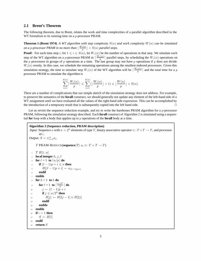
Let us revisit the sequence reduction example, and try to write the barebones PRAM algorithm for a p-processorPRAM, following the simulation strategy described. Each forall construct of Algorithm 2 is simulated using a sequen-tial for loop with a body that applies up to p operations of the forall body at a time.

Algorithm 3 (Sequence reduction, PRAM description)Input: Sequence a with n = 2k elements of type T , binary associative operator⊕ :T ×T → T , and processor

id i.Output: S = ⊕n

i=1ai.

T PRAM-REDUCE(sequence〈T〉 a, ⊕ :T × T → T )

1 T B[1..n]2 local integer h, j, �3 for � = 1 to �n/p� do4 if (�− 1)p+ i � n then5 B[(�− 1)p+ i] ← a(�−1)p+i

6 endif7 enddo8 for h = 1 to k do

9 for � = 1 to � n/2h

p � do10 j ← (�− 1)p+ i11 if j � n/2h then12 B[j] ← B[2j − 1]⊕B[2j]13 endif14 enddo15 enddo16 if i = 1 then17 S ← B[1]18 endif19 return S

5

The concurrent running time of Algorithm 3 can be analyzed by counting the number of executions of the loopbodies.

TC(n, p) = �np�Θ(1) +

k∑h=1

�n/2h

p�Θ(1) + Θ(1) = O(

n

p+ lgn)

This is the bound provided by Brent’s theorem for the simulation of Algorithm 2 with a p processor PRAM. To verifythat the bound is tight, consider the summation above in the case that p > n or the case that p is odd. With some minorassumptions, the simulation preserves the shared-memory access model, so that, for example, an EREW algorithm inthe WT framework can be simulated using an EREW PRAM.

2.2 Designing good parallel algorithms

PRAM algorithms have a time complexity in which both problem size and the number of processors are parameters.Given a PRAM algorithm with running time TC(n, p), let TS(n) be the optimal (or best known) sequential timecomplexity for the problem. We define the speedup

SP(n, p) =TS(n)TC(n, p)

(2)

as the factor of improvement in the running time due to parallel execution. The best speedup we can hope to achieve(for a deterministic algorithm) is Θ(p) when using p processors. An asymptotically greater speedup would contra-dict the assumption that our sequential time complexity was optimal, since a faster sequential algorithm could beconstructed by sequential simulation of our PRAM algorithm.

Parallel algorithms in the WT framework are characterized by the single-parameter step and work complexitymeasures. The work complexity W (n) is the most critical measure. By Brent’s Theorem, we can simulate a WTalgorithm on a p-processor PRAM in time

TC(n, p) = O(W (n)p

+ S(n)). (3)

IfW (n) asymptotically dominatesTS(n), then we can see that with a fixed number of processors p, increasing problemsize decreases the speedup, i.e.

limn→∞SP(n, p) = lim

n→∞TS(n)

�W (n)p �+ S(n)

= 0

Since scaling of p has hard limits in many real settings, we will want to construct parallel WT algorithms for whichW (n) = Θ(TS(n)). Such algorithms are called work-efficient.

The second objective is to minimize step complexity S(n). By Brent’s Theorem, we can simulate a work-efficientWT algorithm on a p-processor PRAM in time

TC(n, p) = O(TS(n)p

+ S(n)). (4)

Thus, the speedup achieved on the p-processor PRAM is

SP(n, p) = Ω(TS(n)

TS(n)p + S(n)

) = Ω(pTS(n)

TS(n) + pS(n)). (5)

Thus, SP(n, p) will be Θ(p) (asymptotically the best we can achieve) as long as

p = O(TS(n)S(n)

). (6)

Thus, among two work-efficient parallel algorithms for a problem, the one with the smaller step complexity is morescalable in that it maintains optimal speedup over a larger range of processors.

6

3 Basic PRAM algorithm design techniques

We now discuss a variety of algorithm design techniques for PRAMs. As you will see, these techniques can deal withmany different kinds of data structures, and often have counterparts in design techniques for sequential algorithms.

3.1 Balanced trees

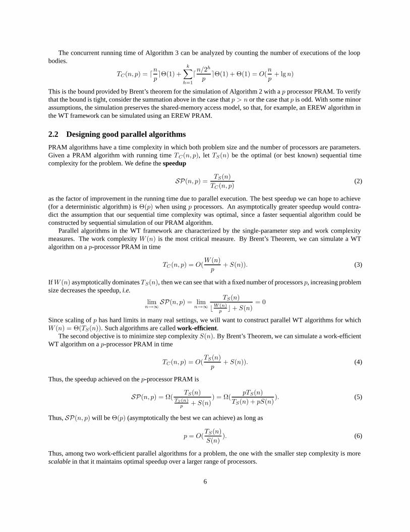
One common PRAM algorithm design technique involves building a balanced binary tree on the input data and sweep-ing this tree to and from the root. This “tree” is not an actual data structure but rather a concept in our head, oftenrealized as a recursion tree. We have already seen a use of this technique in the array summation example. Thistechnique is widely applicable. It is used to construct work-efficient parallel algorithms for problems such as prefixsum, broadcast, and array compaction. We will look at the prefix sum case.

In the prefix sum problem (also called parallel prefix or scan), we are given an input sequence x = 〈x 1, . . . , xn〉 ofelements of some type T , and a binary associative operator⊕ :T ×T → T . As output, we are to produce the sequences = 〈s1, . . . , sn〉, where for 1 � k � n, we require that sk = ⊕k

i=1xi.The sequential time complexity TS(n) of the problem is clearly Θ(n): the lower bound follows trivially from the

fact that n output elements have to be written, and the upper bound is established by the algorithm that computes s i+1

as si ⊕ xi+1. Thus, our goal is to produce a parallel algorithm with work complexity Θ(n). We will do this using thebalanced tree technique. Our WT algorithm will be different from previous ones in that it is recursive. As usual, wewill assume that n = 2k to simplify the presentation.

Algorithm 4 (Prefix sum)Input: Sequence x of n = 2k elements of type T , binary associative operator⊕ :T × T → T .Output: Sequence s of n = 2k elements of type T , with sk = ⊕k

i=1xi for 1 � k � n.

sequence〈T〉 SCAN(sequence〈T〉 x, ⊕ :T × T → T )

1 if n = 1 then2 s1 ← x1

3 return s4 endif5 forall i ∈ 1 :n/2 do6 yi ← x2i−1 ⊕ x2i

7 enddo8 〈z1, . . . , zn/2〉 ← SCAN(〈y1, . . . , yn/2〉, ⊕)9 forall i ∈ 1 :n do

10 if even(i) then11 si ← zi/2

12 elsif i = 1 then13 s1 ← x1

14 else15 si ← z(i−1)/2 ⊕ xi

16 endif17 enddo18 return s

Figure 1 illustrates the data flow of Algorithm 4.

Theorem 2 Algorithm 4 correctly computes the prefix sum of the sequence x with step complexity Θ(lg n) and workcomplexity Θ(n).

7

Y

Recursion

Z

S

X

Figure 1: Data flow in Algorithm 4 for an example input of eight elements.

Proof: The correctness of the algorithm is a simple induction on k = lg n. The base case is k = 0, which is correctby line 2. Now assume the correctness for inputs of size 2k, and consider an input of size 2k+1. By the inductionhypothesis, z = SCAN(y, ⊕) computed in line 8 is correct. Thus, z i = y1 ⊕ · · · ⊕ yi = x1 ⊕ · · · ⊕ x2i. Now considerthe three possibilities for si. If i = 2j is even (line 11), then si = zj = x1 ⊕ · · · ⊕ x2j = x1 ⊕ · · · ⊕ xi. If i = 1(line 13), then s1 = x1. Finally, if i = 2j + 1 is odd (line 15), then si = zj ⊕ xi = x1 ⊕ · · · ⊕ xi−1 ⊕ xi. These threecases are exhaustive, thus establishing the correctness of the algorithm.

To establish the resource bounds, we note that the step and work complexities satisfy the following recurrences.

S(n) = S(n/2) + Θ(1) (7)

W (n) = W (n/2) + Θ(n) (8)

These are standard recurrences that solve to S(n) = Θ(lgn) and W (n) = Θ(n). �

Thus we have a work-efficient parallel algorithm that can run on an EREW PRAM. It can maintain optimal speedupwith O( n

lg n ) processors.Why is the minimal PRAM model EREW when there appears to be a concurrent read of values in z[1 :n/2 − 1]

(as suggested by Figure 1)? It is true that each of these values must be read twice, but these reads can be serializedwithout changing the asymptotic complexity of the algorithm. In fact, since the reads occur on different branches ofthe conditional (lines 11 and 15), they will be serialized in execution under the synchronous PRAM model. In the nextsection, we will see an example where more than a constant number of processors are trying to read a common value,making the minimal PRAM model CREW.

We can define two variants of the scan operation: inclusive (as above) and exclusive. For the exclusive scan, werequire that the operator ⊕ have an identity element I . (This means that x ⊕ I = I ⊕ x = x for all elements x.)The exclusive scan is then defined as follows: if t is the output sequence, then t 1 = I and tk = x1 ⊕ · · · ⊕ xk−1 for1 < k � n. It is clear that we can obtain the inclusive scan from the exclusive scan by the relation s k = tk ⊕ xk.Going in the other direction, observe that for k > 1, tk = sk−1 and t1 = I .

8

Finally, what do we do if n �= 2k? If 2k < n < 2k+1, we can simply pad the input to size 2k+1, use Algorithm 4,and discard the extra values. Since this does not increase the problem size by more than a factor of two, we maintainthe asymptotic complexity.

3.2 Pointer jumping

The technique of pointer jumping (or pointer doubling) allows fast parallel processing of linked data structures suchas lists and trees. We will usually draw trees with edges directed from children to parents (as we do in representingdisjoint sets, for example). Recall that a rooted directed tree T is a directed graph with a special root vertex r such thatthe outdegree of the root is zero, while the outdegree of all other vertices is one, and there exists a directed path fromeach non-root vertex to the root vertex. Our example problem will be to find all the roots of a forest of directed trees,containing a total of n vertices (and at most n− 1 edges).

We will represent the forest using an array P (for “Parent”) of n integers, such that P [i] = j if and only if (i, j)is an edge in the forest. We will use self-loops to recognize roots, i.e., a vertex i is a root if and only if P [i] = i. Thedesired output is an array S, such that S[j] is the root of the tree containing vertex j, for 1 � j � n. A sequentialalgorithm using depth-first search gives TS(n) = O(n).

Algorithm 5 (Roots of a forest)Input: A forest on n vertices represented by the parent array P [1..n].Output: An array S[1..n] giving the root of the tree containing each vertex.

1 forall i ∈ 1 :n do2 S[i] ← P [i]3 while S[i] �= S[S[i]] do4 S[i] ← S[S[i]]5 endwhile6 enddo

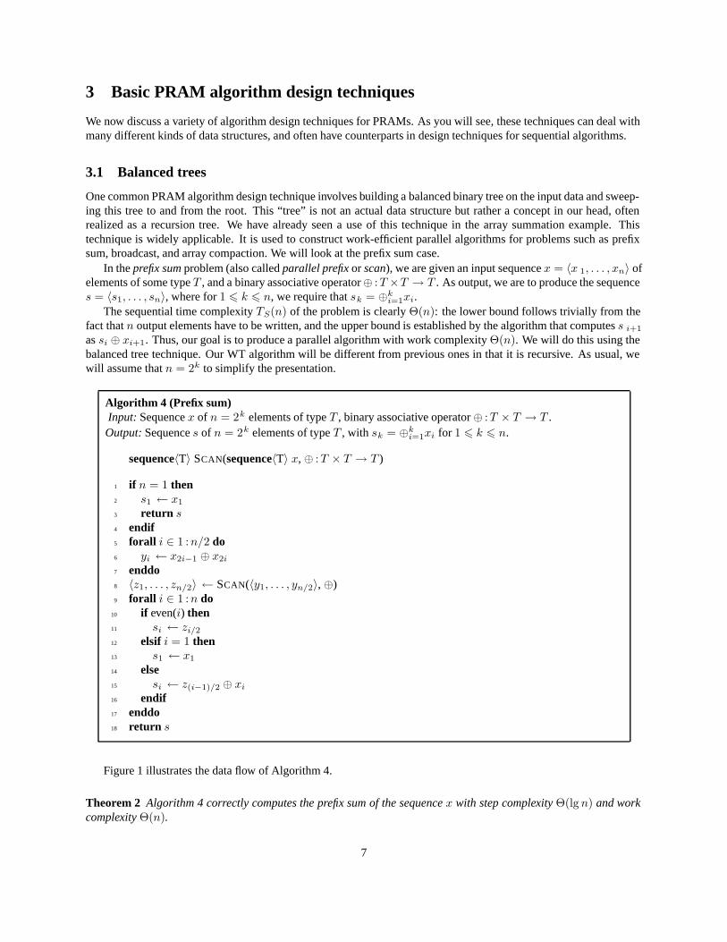
Note again that in line 4 all instances of S[S[i]] are evaluated before any of the assignments to S[i] are performed.The pointer S[i] is the current “successor” of vertex i, and is initially its parent. At each step, the tree distance betweenvertices i and S[i] doubles as long as S[S[i]] is not a root of the forest. Let h be the maximum height of a treein the forest. Then the correctness of the algorithm can be established by induction on h. The algorithm runs ona CREW PRAM. All the writes are distinct, but more than a constant number of vertices may read values from acommon vertex, as shown in Figure 2. To establish the step and work complexities of the algorithm, we note that thewhile-loop iterates Θ(lg h) times, and each iteration performs Θ(1) steps andO(n) work. Thus, S(n) = Θ(lg h), andW (n) = O(n lg h). These bounds are weak, but we cannot assert anything stronger without assuming more aboutthe input data. The algorithm is not work-efficient unless h is constant. In particular, for a linked list, the algorithmtakes Θ(lgn) steps and Θ(n lg n) work. An interesting exercise is to associate with each vertex i the distance d i toits successor measured along the path in the tree, and to modify the algorithm to correctly maintain this quantity. Ontermination, the di will be the distance of vertex i from the root of its tree.

The algorithm glosses over one important detail: how do we know when to stop iterating the while-loop? The firstidea is to use a fixed iteration count, as follows. Since the height of the tallest tree has a trivial upper bound of n, wedo not need to repeat the pointer jumping loop more than lg n times.

forall i ∈ 1 :n doS[i] ← P [i]

enddofor k = 1 to lgn do

forall i ∈ 1 :n doS[i] ← S[S[i]]

enddoenddo

9

1 2

4 5

6 7

8

9

10

11

12

13

3

1 2

4 5

6 7

8

9

10

11

12

13

3

1 2

4 5

6 7

8

9

10

11

12

13

3

Figure 2: Three iterations of line 4 in Algorithm 5 on a forest with 13 vertices and two trees.

10

This is correct but inefficient, since our forest might consist of many shallow and bushy trees. Its work complexity isΘ(n lgn) instead of O(n lg h), and its step complexity is Θ(lgn) instead of O(lg h). The second idea is an “honest”termination detection algorithm, as follows.

forall i ∈ 1 :n doS[i] ← P [i]

enddorepeat

forall i ∈ 1 :n doS[i] ← S[S[i]]M [i] ← if S[i] �= S[S[i]] then 1 else 0 endif

enddot ← REDUCE(M , +)

until t = 0

This approach has the desired work complexity of O(n lg h), but its step complexity is O(lg n lg h), since we performan O(lg n) step reduction in each of the lg h iterations.

In the design of parallel algorithms, minimizing work complexity is most important, hence we would probablyfavor the use of the honest termination detection in Algorithm 5. However, the basic algorithm, even with this mod-ification, is not fully work efficient. The algorithm can be made work efficient using the techniques presented in thenext section; details may be found in JaJa §3.1.

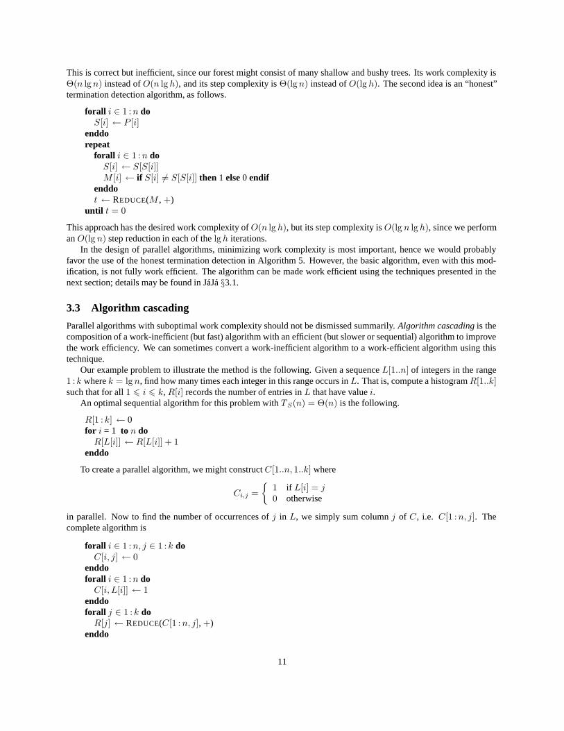
3.3 Algorithm cascading

Parallel algorithms with suboptimal work complexity should not be dismissed summarily. Algorithm cascading is thecomposition of a work-inefficient (but fast) algorithm with an efficient (but slower or sequential) algorithm to improvethe work efficiency. We can sometimes convert a work-inefficient algorithm to a work-efficient algorithm using thistechnique.

Our example problem to illustrate the method is the following. Given a sequence L[1..n] of integers in the range1 :k where k = lg n, find how many times each integer in this range occurs in L. That is, compute a histogramR[1..k]such that for all 1 � i � k, R[i] records the number of entries in L that have value i.

An optimal sequential algorithm for this problem with TS(n) = Θ(n) is the following.

R[1 :k] ← 0for i = 1 to n doR[L[i]] ← R[L[i]] + 1

enddo

To create a parallel algorithm, we might construct C[1..n, 1..k] where

Ci,j ={

1 if L[i] = j0 otherwise

in parallel. Now to find the number of occurrences of j in L, we simply sum column j of C, i.e. C[1 :n, j]. Thecomplete algorithm is

forall i ∈ 1 :n, j ∈ 1 :k doC[i, j] ← 0

enddoforall i ∈ 1 :n doC[i, L[i]] ← 1

enddoforall j ∈ 1 :k doR[j] ← REDUCE(C[1 :n, j], +)

enddo

11

The step complexity of this algorithm is Θ(lgn) as a result of the step complexity of the REDUCE operations. Thework complexity of the algorithm is Θ(nk) = Θ(n lg n) as a result of the first and last forall constructs. The algorithmis not work efficient because C is too large to initialize and too large to sum up with only O(n) work.

However, a variant of the efficient sequential algorithm given earlier can create and sum k successive rows of C inO(k) = O(lg n) (sequential) steps and work. Using m = n/ lgn parallel applications of this sequential algorithm wecan create C[1..m, 1..k] in O(k) = O(lg n) steps and performing a total of O(mk) = O(n) work. Subsequently wecan compute the column sums of C with these same complexity bounds.

Algorithm 6 (Work-efficient cascaded algorithm for label counting problem)Input: Sequence L[1..n] with values in the range 1 :kOutput: SequenceR[1..k] the occurrence counts for the values in L

1 integer C[1..m, 1..k]2 forall i ∈ 1 :m, j ∈ 1 : k do3 C[i, j] ← 04 enddo5 forall i ∈ 1 :m do6 for j = 1 to k do7 C[i, L[(i− 1)k + j]] ← C[i, L[(i− 1)k + j]] + 18 enddo9 enddo

10 forall j ∈ 1 : k do11 R[j] ← REDUCE(C[1 :m, j], +)12 enddo

The cascaded algorithm has S(n) = O(lg n) and W (n) = O(n) hence has been made work efficient without anasymptotic increase in step complexity. The algorithm runs on the EREW PRAM model.

3.4 Euler tours

The Euler tour technique is used in various parallel algorithms operating on tree-structured data. The name comesfrom Euler circuits of directed graphs. Recall that an Euler circuit of a directed graph is a directed cycle that traverseseach edge exactly once. If we take a tree T = (V,E) and produce a directed graph T ′ = (V,E′) by replacing eachedge (u, v) ∈ E with two directed edges (u, v) and (v, u) in E ′, then the graph T ′ has an Euler circuit. We call aEuler circuit of T ′ an Euler tour of T . Formally, we specify an Euler tour of T by defining a successor functions :E′ → E′, such that s(e) is the edge following edge e in the tour. By defining the successor function appropriately,we can create an Euler tour to enumerate the vertices according to an inorder, preorder or postorder traversal.

For the moment, consider rooted trees. There is a strong link between the Euler tour representation of a treeand a representation of the tree structure as a balanced parenthesis sequence. Recall that every sequence of balancedparentheses has an interpretation as a rooted tree. This representation has the key property that the subsequencerepresenting any subtree is also balanced. The following is a consequence of this property: if⊕ is a binary associativeoperator with an inverse, and we place the element e at each left parenthesis and its inverse element −e at each rightparenthesis, then the sum (with respect to ⊕) of the elements of any subtree is zero.

12

1

25 6

7 8 93 4

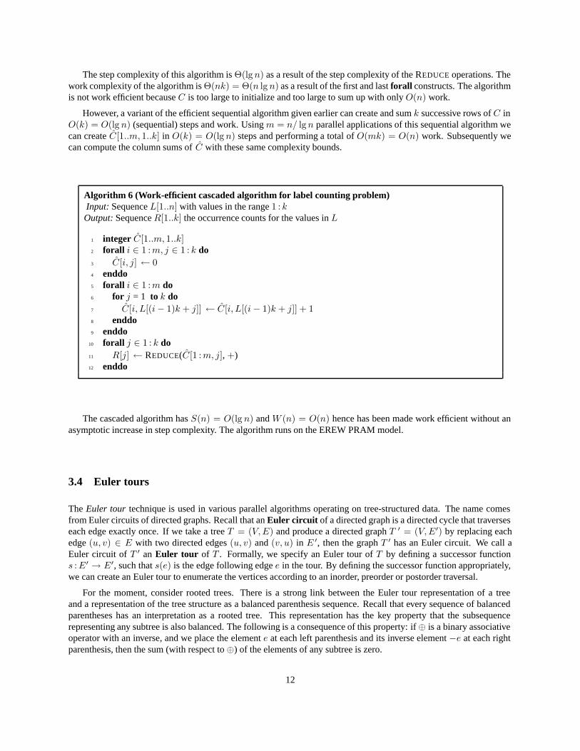
L = 1 2 3 5 8 10 11 13 15R = 18 7 4 6 9 17 12 14 16A = 1 1 1 −1 1 −1 −1 1 −1 1 1 −1 1 −1 1 −1 −1 −1B = 0 1 2 3 2 3 2 1 2 1 2 3 2 3 2 3 2 1D = 0 1 2 2 1 1 2 2 2

Figure 3: Determining the depth of the vertices of a tree.

Algorithm 7 (Depth of tree vertices)Input: A rooted tree T on n vertices in Euler tour representation using two arrays L[1..n] and R[1..n].Output: The array D[1..n] containing the depth of each vertex of T .

1 integer A[1..2n]2 forall i ∈ 1 :n do3 A[L[i]] ← 14 A[R[i]] ←−15 enddo6 B ← EXCL-SCAN(A,+)7 forall i ∈ 1 :n do8 D[i] ← B[L[i]]9 enddo

Algorithm 7 shows how to use this property to obtain the depth of each vertex in the tree. For this algorithm, the treeT with n vertices is represented as two arrays L and R of length n in shared memory (for left parentheses and rightparentheses, respectively). These arrays need to be created from an Euler tour that starts and ends at the root. L i is theearliest position in the tour in which vertex i is visited. R i is the latest position in the tour in which vertex i is visited.

Figure 3 illustrates the operation of Algorithm 7. The algorithm runs on an EREW PRAM with step complexityΘ(lgn) and work complexity Θ(n).

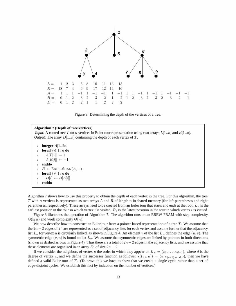
We now describe how to construct an Euler tour from a pointer-based representation of a tree T . We assume thatthe 2n− 2 edges of T ′ are represented as a set of adjacency lists for each vertex and assume further that the adjacencylist Lu for vertex u is circularly linked, as shown in Figure 4. An element v of the list L u defines the edge (u, v). Thesymmetric edge (v, u) is found on list Lv. We assume that symmetric edges are linked by pointers in both directions(shown as dashed arrows in Figure 4). Thus there are a total of 2n−2 edges in the adjacency lists, and we assume thatthese elements are organized in an array E ′ of size 2n− 2.

If we consider the neighbors of vertex u the order in which they appear on L u = (v0, . . . , vd−1), where d is thedegree of vertex u, and we define the successor function as follows: s((v i, u)) = (u, v(i+1) mod d), then we havedefined a valid Euler tour of T . (To prove this we have to show that we create a single cycle rather than a set ofedge-disjoint cycles. We establish this fact by induction on the number of vertices.)

13

2

5

4

3

1 2 2 1 1

7

8

9

6 6 6

6

1

25 6

7 8 93 4

Figure 4: Building the Euler tour representation of a tree from a pointer-based representation.

The successor function can be evaluated in parallel for each edge in E ′ by following the symmetric (dashed)pointer and then the adjacency list (solid) pointer. This requires Θ(1) steps with Θ(n) work complexity, which iswork-efficient. Furthermore, since the two pointers followed for each element in E ′ are unique, we can do this on anEREW PRAM.

Note that what we have accomplished is to link the edges of T ′ into an Euler tour. To create a representation likethe L and R array used in Algorithm 7, we must do further work.

3.5 Divide and conquer

The divide-and-conquer strategy is the familiar one from sequential computing. It has three steps: dividing the probleminto sub-problems, solving the sub-problems recursively, and combining the sub-solutions to produce the solution. Asalways, the first and third steps are critical.

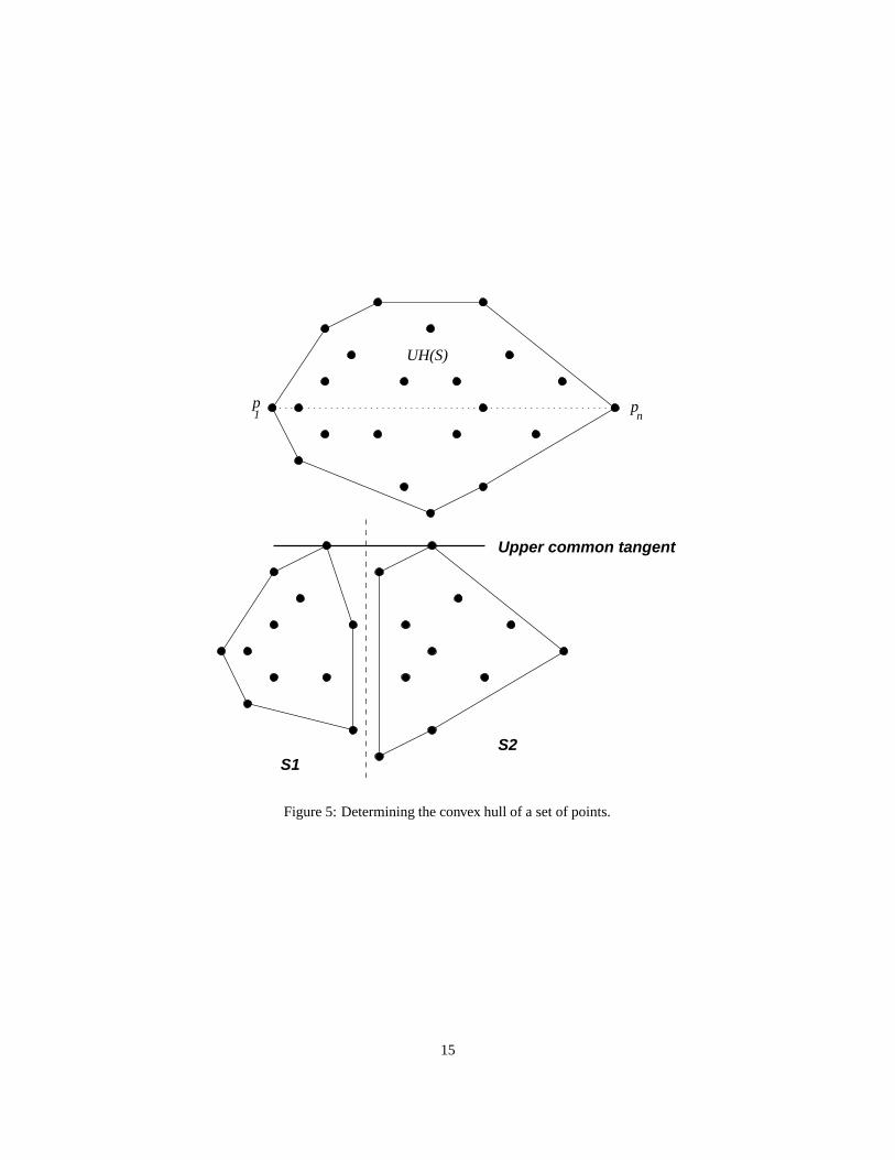
To illustrate this strategy in a parallel setting, we consider the planar convex hull problem. We are given a setS = {p1, . . . , pn} of points, where each point pi is an ordered pair of coordinates (xi, yi). We further assume thatpoints are sorted by x-coordinate. (If not, this can be done as a preprocessing step with low enough complexitybounds.) We are asked to determine the convex hull CH(S), i.e., the smallest convex polygon containing all the pointsof S, by enumerating the vertices of this polygon in clockwise order. Figure 5 shows an instance of this problem.

The sequential complexity of this problem is TS(n) = Θ(n lgn). Any of several well-known algorithms for thisproblem establishes the upper bound. A reduction from comparison-based sorting establishes the lower bound. See§35.3 of CLR for details.

We first note that p1 and pn belong to CH(S) by virtue of the sortedness of S, and they partition the convex hullinto an upper hull UH(S) and an lower hull LH(S). Without loss of generality, we will show how to compute UH(S).

The division step is simple: we partition S into S1 = {p1, . . . , pn/2} and S2 = {pn/2+1, . . . , pn}. We thenrecursively obtain UH(S1) = 〈p1 = q1, . . . , qs〉 and UH(S2) = 〈r1, . . . , rt = pn〉. Assume that for n � 4, we solve theproblem by brute force. This gives us the termination condition for the recursion.

The combination step is nontrivial. Let the upper common tangent (UCT) be the common tangent to UH(S 1)and UH(S2) such that both UH(S1) and UH(S2) are below it. Thus, this tangent consists of two points, one eachfrom UH(S1) and UH(S2). Let UCT(S1, S2) = (qi, rj). Assume the existence of an O(lg n) sequential algorithmfor determining UCT(S1, S2) (See Preparata and Shamos, Lemma 3.1). Then UH(S) = 〈q 1, . . . , qi, rj , . . . , rt〉, andcontains (i+ t− j + 1) points. Given s, t, i, and j, we can obtain UH(S) in Θ(1) steps and O(n) work as follows.

forall k ∈ 1 : i+ t− j + 1 doUH(S)k ← if k � i then qk else rk+j−i−1 endif

14

p1

pn

UH(S)

Upper common tangent

S1S2

Figure 5: Determining the convex hull of a set of points.

15

enddo

This algorithm requires a minimal model of a CREW PRAM. To analyze its complexity, we note that

S(n) = S(n/2) +O(lg n) (9)

W (n) = 2W (n/2) +O(n) (10)

giving us S(n) = O(lg2 n) and W (n) = O(n lg n).

3.6 Symmetry breaking

The technique of symmetry breaking is used in PRAM algorithms to distinguish between identical-looking elements.This can be deterministic or probabilistic. We will study a randomized algorithm (known as the random mate algo-rithm) to determine the connected components of an undirected graph as an illustration of this technique. See §30.5 ofCLR for an example of a deterministic symmetry breaking algorithm.

Let G = (V,E) be an undirected graph. We say that edge (u, v) hits vertices u and v. The degree of a vertex v isthe number of edges that hit v. A path from v1 to vk (denoted v1 � vk) is a sequence of vertices (v1, . . . , vk) suchthat (vi, vi+1) ∈ E for 1 � i < k. A connected subgraph is a subset U of V such that for all u, v ∈ U we have u� v.A connected component is a maximal connected subgraph. A supervertex is a directed rooted tree data structure usedto represent a connected subgraph. We use the standard disjoint-set conventions of edges directed from children toparents and self-loops for roots to represent supervertices.

We can find connected components optimally in a sequential model using depth-first search. Thus, T S(V,E) =O(V + E). Our parallel algorithm will actually be similar to the algorithm in §22.1 of CLR. The idea behind thealgorithm is to merge supervertices to get bigger supervertices. In the sequential case, we examine the edges in apredetermined order. For our parallel algorithm, we would like to examine multiple edges at each time step. We breaksymmetry by arbitrarily choosing the next supervertex to merge, by randomly assigning genders to supervertices. Wecall a graph edge (u, v) live if u and v belong to different supervertices, and we call a supervertex live if at least onelive edge hits some vertex of the supervertex. While we still have live edges, we will merge supervertices of oppositegender connected by a live edge. This merging includes a path compression step. When we run out of live edges, wehave the connected components.

16

u v

M F

parent[u]

parent[v]

u v

parent[v]

parent[u]

u v

parent[v]

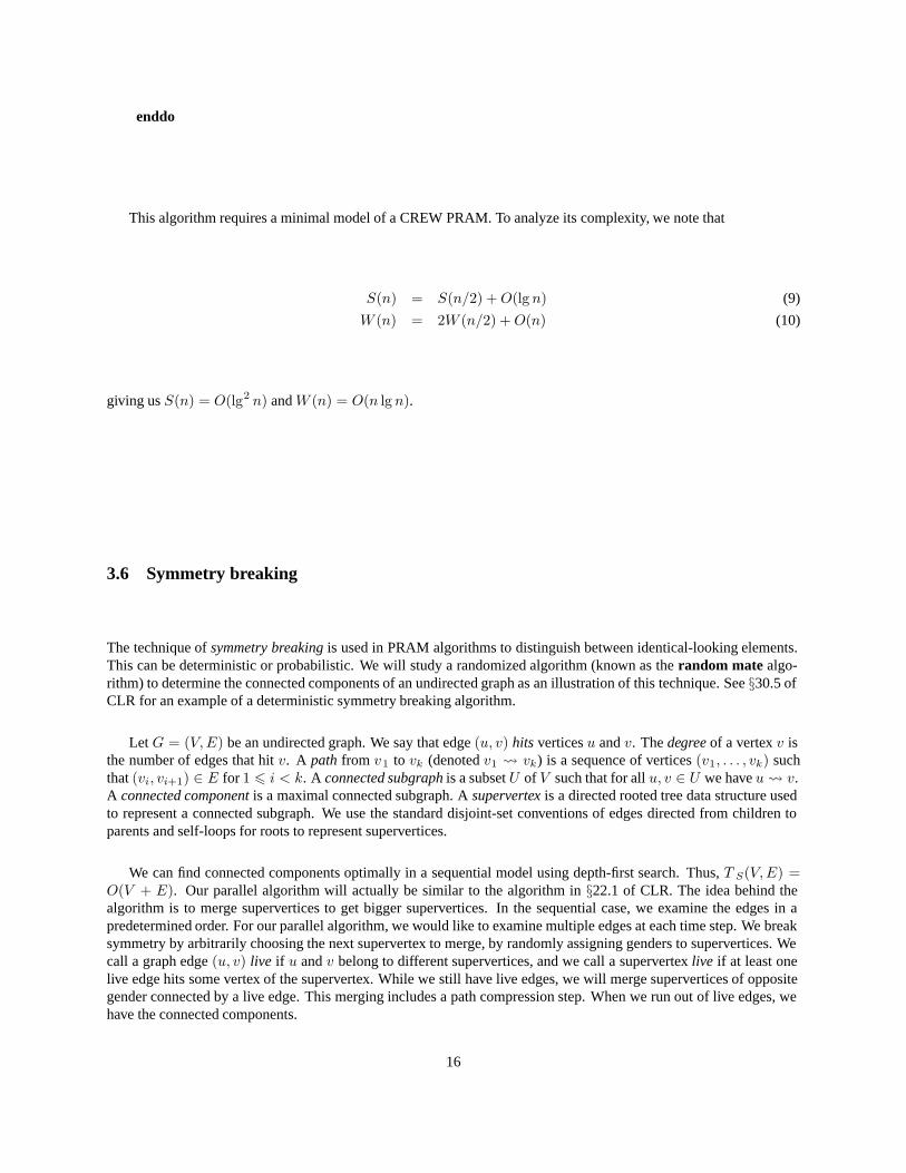
Figure 6: Details of the merging step of Algorithm 8. Graph edges are undirected and shown as dashed lines. Super-vertex edges are directed and are shown as solid lines.

Algorithm 8 (Random-mate algorithm for connected components)Input: An undirected graph G = (V,E).Output: The connected components of G, numbered in the array P [1..|V |].

1 forall v ∈ V do2 parent[v] ← v3 enddo4 while there are live edges in G do5 forall v ∈ V do6 gender[v] = rand({M, F})7 enddo8 forall (u, v) ∈ E | live(u, v) do9 if gender[parent[u]] = M and gender[parent[v]] = F then

10 parent[parent[u]] ← parent[v]11 endif12 if gender[parent[v]] = M and gender[parent[u]] = F then13 parent[parent[v]] ← parent[u]14 endif15 enddo16 forall v ∈ V do17 parent[v] ← parent[parent[v]]18 enddo19 endwhile

Figure 6 shows the details of the merging step of Algorithm 8. We establish the complexity of this algorithm byproving a succession of lemmas about its behavior.

Lemma 1 After each iteration of the outer while-loop, each supervertex is a star (a tree of height zero or one).

Proof: The proof is by induction on the number of iterations executed. Before any iterations of the loop have beenexecuted, each vertex is a supervertex with height zero by the initialization in line 2. Now assume that the claim holdsafter k iterations, and consider what happens in the (k + 1)st iteration. Refer to Figure 6. After the forall loop inline 8, the height of a supervertex can increase by one, so it is at most two. After the compression step in line 16, theheight goes back to one from two. �

Lemma 2 Each iteration of the while-loop takes Θ(1) steps and O(V + E) work.

17

Proof: This is easy. The only nonobvious part is determining live edges, which can be done in Θ(1) steps and O(E)work. Since each vertex is a star by Lemma 1, edge (u, v) is live if and only if parent[u] �= parent[v]. �

Lemma 3 The probability that at a given iteration a live supervertex is joined to another supervertex � 1/4.

Proof: A live supervertex has at least one live edge. The supervertex will get a new root if and only if its gender isM and it has a live edge to a supervertex whose gender is F. The probability of this is 1

2 · 12 = 1

4 . The probability is atleast this, since the supervertex may have more than one live edge. �

Lemma 4 The probability that a vertex is a live root after 5 lg |V | iterations of the while-loop is � 1/|V |2.

Proof: By Lemma 3, a live supervertex at iteration i has probability� 34 to remain live after iteration i+1. Therefore

the probability that it is lives after 5 lg |V | iterations is � ( 34 )5 lg |V |. The inequality follows, since lg( 3

4 )5 lg |V | =−2.075 lg |V | and lg 1

|V |2 = −2 lg |V |. �

Lemma 5 The expected number of live supervertices after 5 lg |V | iterations� 1/|V |.Proof: We compute the expected number of live supervertices by summing up the probability of each vertex to be alive root. By Lemma 4, this is � |V | · 1

|V |2 = 1|V | . �

Theorem 3 With probability at most 1/|V |, the algorithm will not have terminated after 5 lg |V | iterations.

Proof: Let pk be the probability of having k live supervertices after 5 lg |V | iterations. By the definition of expectation,

the expected number of live supervertices after 5 lg |V | iterations is∑|V |

k=0 k ·pk, and by Lemma 5, this is� 1|V | . Since

k and pk are all positive,∑|V |

k=1 pk �∑|V |

k=0 k · pk � 1|V | . Now, the algorithm terminates when the number of live

supervertices is zero. Therefore,∑|V |

k=1 pk is the probability of still having to work after 5 lg |V | steps. �

The random mate algorithm requires a CRCW PRAM model. Concurrent writes occur in the merging step (line 8),since different vertices can have a common parent.

The step complexity of the algorithm is O(lg V ) with high probability, as a consequence of Theorem 3. The workcomplexity is O((V + E) lg V ) by Theorem 3 and Lemma 2. Thus the random mate algorithm is not work-optimal.

A key factor in this algorithm is that paths in supervertices are short (in fact, Θ(1)). This allows the superverticesafter merging to be converted back to stars in a single iteration of path compression in line 16. If we used somedeterministic algorithm to break symmetry, we would not be able to guarantee short paths. We would have multiplesupervertices and long paths within supervertices, and the step complexity of such an algorithm would be O(lg 2 V ).There is a deterministic algorithm due to Shiloach and Vishkin that avoids this problem by not doing complete pathcompression at each step. Instead, it maintains a complicated set of invariants that insure that the supervertices leftwhen the algorithm terminates truly represent the connected components.

4 A tour of data-parallel algorithms

In this section, we present a medley of data-parallel algorithms for some common problems.

4.1 Basic scan-based algorithms

A number of useful building blocks can be constructed using the scan operation as a primitive. In the followingexamples, we will use both zero-based and one-based indexing of arrays. In each case, be sure to calculate step andwork complexities and the minimum PRAM model required.

18

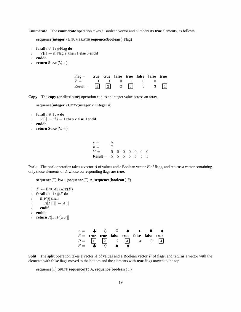
Enumerate The enumerate operation takes a Boolean vector and numbers its true elements, as follows.

sequence〈integer 〉 ENUMERATE(sequence〈boolean 〉 Flag)

1 forall i ∈ 1 : #Flag do2 V[i] ← if Flag[i] then 1 else 0 endif3 enddo4 return SCAN(V, +)

Flag = true true false true false false trueV = 1 1 0 1 0 0 1Result = 1 2 2 3 3 3 4

Copy The copy (or distribute) operation copies an integer value across an array.

sequence〈integer 〉 COPY(integer v, integer n)

1 forall i ∈ 1 :n do2 V [i] ← if i = 1 then v else 0 endif3 enddo4 return SCAN(V, +)

v = 5n = 7V = 5 0 0 0 0 0 0Result = 5 5 5 5 5 5 5

Pack The pack operation takes a vectorA of values and a Boolean vector F of flags, and returns a vector containingonly those elements of A whose corresponding flags are true.

sequence〈T〉 PACK(sequence〈T〉 A, sequence〈boolean 〉 F)

1 P ← ENUMERATE(F )2 forall i ∈ 1 : #F do3 if F [i] then4 R[P [i]] ← A[i]5 endif6 enddo7 return R[1 :P [#F ]]

A = ♣ ♦ ♥ ♠ � � �F = true true false true false false trueP = 1 2 2 3 3 3 4R = ♣ ♦ ♠ �

Split The split operation takes a vector A of values and a Boolean vector F of flags, and returns a vector with theelements with false flags moved to the bottom and the elements with true flags moved to the top.

sequence〈T〉 SPLIT(sequence〈T〉 A, sequence〈boolean 〉 F)

19

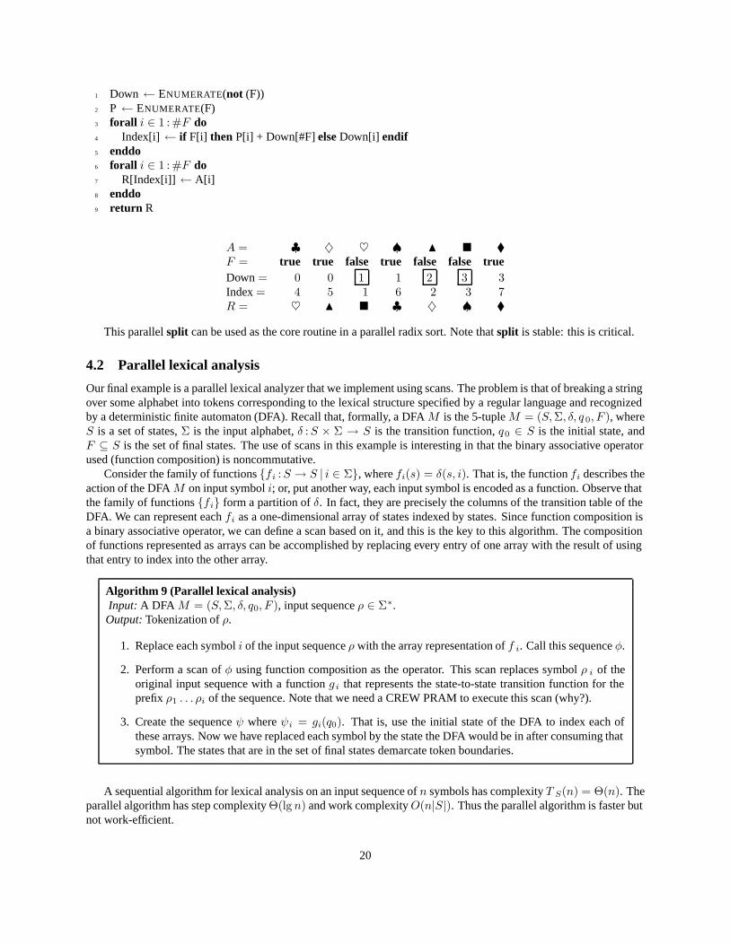
1 Down ← ENUMERATE(not (F))2 P ← ENUMERATE(F)3 forall i ∈ 1 : #F do4 Index[i] ← if F[i] then P[i] + Down[#F] else Down[i] endif5 enddo6 forall i ∈ 1 : #F do7 R[Index[i]] ← A[i]8 enddo9 return R

A = ♣ ♦ ♥ ♠ � � �F = true true false true false false trueDown = 0 0 1 1 2 3 3Index = 4 5 1 6 2 3 7R = ♥ � � ♣ ♦ ♠ �

This parallel split can be used as the core routine in a parallel radix sort. Note that split is stable: this is critical.

4.2 Parallel lexical analysis

Our final example is a parallel lexical analyzer that we implement using scans. The problem is that of breaking a stringover some alphabet into tokens corresponding to the lexical structure specified by a regular language and recognizedby a deterministic finite automaton (DFA). Recall that, formally, a DFA M is the 5-tuple M = (S,Σ, δ, q 0, F ), whereS is a set of states, Σ is the input alphabet, δ :S × Σ → S is the transition function, q0 ∈ S is the initial state, andF ⊆ S is the set of final states. The use of scans in this example is interesting in that the binary associative operatorused (function composition) is noncommutative.

Consider the family of functions {fi :S → S | i ∈ Σ}, where fi(s) = δ(s, i). That is, the function fi describes theaction of the DFA M on input symbol i; or, put another way, each input symbol is encoded as a function. Observe thatthe family of functions {fi} form a partition of δ. In fact, they are precisely the columns of the transition table of theDFA. We can represent each fi as a one-dimensional array of states indexed by states. Since function composition isa binary associative operator, we can define a scan based on it, and this is the key to this algorithm. The compositionof functions represented as arrays can be accomplished by replacing every entry of one array with the result of usingthat entry to index into the other array.

Algorithm 9 (Parallel lexical analysis)Input: A DFA M = (S,Σ, δ, q0, F ), input sequence ρ ∈ Σ∗.Output: Tokenization of ρ.

1. Replace each symbol i of the input sequence ρ with the array representation of f i. Call this sequence φ.

2. Perform a scan of φ using function composition as the operator. This scan replaces symbol ρ i of theoriginal input sequence with a function g i that represents the state-to-state transition function for theprefix ρ1 . . . ρi of the sequence. Note that we need a CREW PRAM to execute this scan (why?).

3. Create the sequence ψ where ψi = gi(q0). That is, use the initial state of the DFA to index each ofthese arrays. Now we have replaced each symbol by the state the DFA would be in after consuming thatsymbol. The states that are in the set of final states demarcate token boundaries.

A sequential algorithm for lexical analysis on an input sequence of n symbols has complexity T S(n) = Θ(n). Theparallel algorithm has step complexity Θ(lg n) and work complexityO(n|S|). Thus the parallel algorithm is faster butnot work-efficient.

20

5 The relative power of PRAM models

We say that a PRAM model P is more powerful than another PRAM model Q if an algorithm with step complexityS(n) on model Q has step complexity O(S(n)) on model P . We show that the ability to perform concurrent readsand writes allows us to solve certain problems faster, and then we quantify just how much more powerful the CREWand CRCW models are compared to the EREW model.

5.1 The power of concurrent reads

How long does it take for p processors of an EREW PRAM to read a value in shared memory? There are two possibleways for the p processors to read the shared value. First, they can serially read the value in round robin fashion inO(p) time. Second, processors can replicate the value as they read it, so that a larger number of processors can read itin the next round. If each processor makes one copy of the value as it reads it, the number of copies doubles at eachround, and O(lg p) time suffices to make the value available to the p processors.

The argument above is, however, only an upper bound proof. We now give a lower bound proof, i.e., an argumentthat Ω(lg p) steps are necessary. Suppose that as each processor reads the value, it sequentially makes k copies, wherek can be a function of p. Then the number of copies grows by a factor of k(p) at each round, but each round takesk(p) time. The number of rounds needed to replicate the value p-fold is lg p/ lg k, and the total time taken is lg p · k

lg k .

This is asymptotically greater than lg p unless klg k = Θ(1), i.e., k is a constant. This means that it is no good trying

to make more copies sequentially at each round. The best we can do is to make a constant number of copies, and thatgives us the desired Ω(lg p) bound. A replication factor of k = 2 gives us the smallest constant, but any constant valueof k will suffice for the lower bound argument.

5.2 The power of concurrent writes

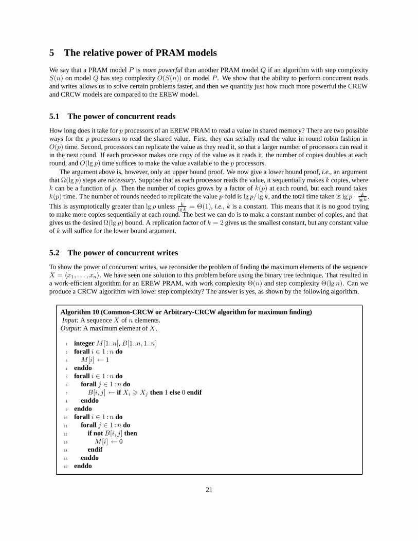
To show the power of concurrent writes, we reconsider the problem of finding the maximum elements of the sequenceX = 〈x1, . . . , xn〉. We have seen one solution to this problem before using the binary tree technique. That resulted ina work-efficient algorithm for an EREW PRAM, with work complexity Θ(n) and step complexity Θ(lg n). Can weproduce a CRCW algorithm with lower step complexity? The answer is yes, as shown by the following algorithm.

Algorithm 10 (Common-CRCW or Arbitrary-CRCW algorithm for maximum finding)Input: A sequence X of n elements.Output: A maximum element of X .

1 integer M [1..n], B[1..n, 1..n]2 forall i ∈ 1 :n do3 M [i] ← 14 enddo5 forall i ∈ 1 :n do6 forall j ∈ 1 :n do7 B[i, j] ← if Xi � Xj then 1 else 0 endif8 enddo9 enddo

10 forall i ∈ 1 :n do11 forall j ∈ 1 :n do12 if not B[i, j] then13 M [i] ← 014 endif15 enddo16 enddo

21

It is easy to verify that M [i] = 1 at the end of this computation if and only if X i is a maximum element. Analysisof this algorithm reveals that S(n) = Θ(1) but W (n) = Θ(n2). Thus the algorithm is very fast but far indeed frombeing work efficient. However, we may cascade this algorithm with the sequential maximum reduction algorithm orthe EREW PRAM maximum reduction algorithm to obtain a work efficient CRCW PRAM algorithm with S(n) =Θ(lg lg n) step complexity. This is optimal for the Common and Arbitrary CRCW model. Note that a trivial work-efficient algorithm with S(n) = Θ(1) exists for maximum value problem in the Combining-CRCW model, whichdemonstrates the additional power of this model.

The Θ(1) step complexity for maximum in CRCW models is suspicious, and points to the lack of realism in theCRCW PRAM model. Nevertheless, a bit-serial maximum reduction algorithm based on ideas like the above butemploying only single-bit concurrent writes (i.e. a wired “or” tree), has proved to be extremely fast and practical in anumber of SIMD machines. The CRCW PRAM model can easily be used to construct completely unrealistic parallelalgorithms, but it remains important because it has also led to some very practical algorithms.

5.3 Quantifying the power of concurrent memory accesses

The CRCW PRAM model assumes that any number of simultaneous memory accesses to the same location can beserved in a single timestep. A real parallel machine will clearly never be able to do that. The CRCW model maybe a powerful model for algorithm design, but it is architecturally implausible. We will try to see how long it takesan EREW PRAM to simulate the concurrent memory accesses of a CRCW PRAM. Specifically, we will deal withconcurrent writes under a priority strategy. We assume the following lemma without proof.

Lemma 6 (Cole 1988) A p-processor EREW PRAM can sort p elements in Θ(lg p) steps. �

Based on this lemma, we can prove the following theorem.

Theorem 4 A p-processor EREW PRAM can simulate a p-processor Priority CRCW PRAM with Θ(lg p) slowdown.

Proof: In fact, all we will show is a simulation that guarantees O(lg p) slowdown. The Ω(lg p) lower bound doeshold, but establishing it is beyond the scope of this course. See Chapter 10 of JaJa if you are interested.

Assume that the CRCW PRAM has p processors P1 through Pp and m memory locations M1 through Mm, andthat the EREW PRAM has the same number of processors but O(p) extra memory locations. We will show howto simulate on the EREW PRAM a CR or CW step in which processor Pi accesses memory location Mj . In oursimulation, we will use an array T to store the pairs (j, i), and an array S to record the processor that finally got theright to access a memory location.

The following code describes the simulation.

22

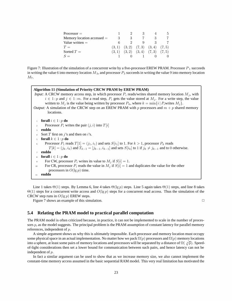
Processor = 1 2 3 4 5Memory location accessed = 3 3 7 3 7Value written = 6 2 9 3 7T = (3, 1) (3, 2) (7, 3) (3, 4) (7, 5)Sorted T = (3, 1) (3, 2) (3, 4) (7, 3) (7, 5)S = 1 0 1 0 0

Figure 7: Illustration of the simulation of a concurrent write by a five-processor EREW PRAM. Processor P 1 succeedsin writing the value 6 into memory locationM3, and processorP3 succeeds in writing the value 9 into memory locationM7.

Algorithm 11 (Simulation of Priority CRCW PRAM by EREW PRAM)Input: A CRCW memory access step, in which processor Pi reads/writes shared memory location Mj , with

i ∈ 1 : p and j ∈ 1 :m. For a read step, Pi gets the value stored at Mj . For a write step, the valuewritten to Mj is the value being written by processor Pk, where k = min{i |Piwrites Mj}.

Output: A simulation of the CRCW step on an EREW PRAM with p processors and m + p shared memorylocations.

1 forall i ∈ 1 : p do2 Processor Pi writes the pair (j, i) into T [i]3 enddo4 Sort T first on j’s and then on i’s.5 forall k ∈ 1 : p do6 Processor P1 reads T [1] = (j1, i1) and sets S[i1] to 1. For k > 1, processor Pk reads

T [k] = (jk, ik) and Tk−1 = [jk−1, ik−1] and sets S[ik] to 1 if jk �= jk−1 and to 0 otherwise.7 enddo8 forall i ∈ 1 : p do9 For CW, processor Pi writes its value to Mj if S[i] = 1.

10 For CR, processor Pi reads the value in Mj if S[i] = 1 and duplicates the value for the otherprocessors in O(lg p) time.

11 enddo

Line 1 takes Θ(1) steps. By Lemma 6, line 4 takes Θ(lg p) steps. Line 5 again takes Θ(1) steps, and line 8 takesΘ(1) steps for a concurrent write access and O(lg p) steps for a concurrent read access. Thus the simulation of theCRCW step runs in O(lg p) EREW steps.

Figure 7 shows an example of this simulation. �

5.4 Relating the PRAM model to practical parallel computation

The PRAM model is often criticized because, in practice, it can not be implemented to scale in the number of proces-sors p, as the model suggests. The principal problem is the PRAM assumption of constant latency for parallel memoryreferences, independent of p.

A simple argument shows us why this is ultimately impossible. Each processor and memory location must occupysome physical space in an actual implementation. No matter how we pack Ω(p) processors and Ω(p) memory locationsinto a sphere, at least some pairs of memory locations and processors will be separated by a distance of Ω( 3

√p). Speed-

of-light considerations then set a lower bound for communication between such pairs, and hence latency can not beindependent of p.

In fact a similar argument can be used to show that as we increase memory size, we also cannot implement theconstant-time memory access assumed in the basic sequential RAM model. This very real limitation has motivated the

23

use of cache memories and the memory hierarchy found in modern processors. And indeed with modern processors,the RAM model is an increasingly inadequate cost model for sequential algorithms as well.

A PRAM implementation suffers from these physical constraints much more than a RAM implementation becauseof the additional components required to implement a PRAM. For example, a p processor PRAM must deliver Ω(p)bandwidth between the memory system and the processors through an interconnection network that is significantlylarger than the processors themselves.

Another limitation on latency in the PRAM results from the implementation of concurrent read and write opera-tions. Current memory components permit at most a constant number of simultaneous reads and writes. As we haveseen in the previous two sections, this means there is an Ω(lg p) latency involved in the servicing of concurrent readsand writes using these memory components.

Nevertheless, a PRAM algorithm can be a valuable start for a practical parallel implementation. Any algorithmthat runs efficiently on a p processor PRAM model can be translated into an algorithm that sacrifices a factor of L inparallelism to run efficiently on a p/L-processor machine with a latency O(L) memory system, a much more realisticmachine than the PRAM. In the translated algorithm, each of the p/L processors simulates L PRAM processors. Thememory latency is “hidden” because a processor has L units of useful and independent work to perform while waitingfor each memory access to complete.

A good example of latency hiding can be found in a classical vector processor supercomputer with a high-bandwidth memory system: the interconnect and memory system are pipelined to deliver an amortized unit latencyfor a stream of L independent memory references (a vector read or write). Latency hiding is also implemented bythe increasingly advanced superscalar and multithreading capabilities incorporated in commodity processors such asimplementations of the Intel IA-32 architecture and the Sun UltraSparc architecture, although generally not anywherenear the scale that can fully amortize the latency in all cases. The memory subsystems are the rate-limiting componentin systems constructed around such processors.

Instead of running a PRAM algorithm on an expensive latency-hiding supercomputer, a PRAM algorithm maysometimes be restructured so its shared memory access requirements are better matched to shared memory multipro-cessors based on conventional processors with caches. This is the topic of the next unit in this course.

24