Praise for Principles of Neural Information...

Praise for Principles of Neural Information Theory.

This is a terrific book, which cannot fail to help any student who wantsto understand precisely how energy and information constrain neuraldesign. The tutorial approach adopted makes it more like a novel thana textbook. Consequently, both mathematically sophisticated readers andreaders who prefer verbal explanations should be able to understand thematerial. Overall, Stone has managed to weave the disparate strands ofneuroscience, psychophysics, and Shannon’s theory of communicationinto a coherent account of neural information theory. I only wish I’dhad this text as a student!Peter Sterling, Professor of Neuroscience, University of Pennsylvania,co-author of Principles of Neural Design.

This excellent book provides an accessible introduction to aninformation theoretic perspective on how the brain works, and (moreimportantly) why it works that way. Using a wide range of examples,including both structural and functional aspects of brain organisation,Stone describes how simple optimisation principles derived fromShannon’s information theory predict physiological parameters (e.g.axon diameter) with remarkable accuracy. These principles are distilledfrom original research papers, and the informal presentation stylemeans that the book can be appreciated as an overview; but fullmathematical details are also provided for dedicated readers. Stone hasintegrated results from a diverse range of experiments, and in so doinghas produced an invaluable introduction to the nascent field of neuralinformation theory.Dr Robin Ince, Institute of Neuroscience and Psychology, University ofGlasgow, UK.

Essential reading for any student of the why of neural coding: why doneurons send signals they way they do? Stone’s insightful, clear, andeminently readable synthesis of classic studies is a gateway to a rich,glorious literature on the brain. Student and professor alike will findmuch to spark their minds within. I shall be keeping this wonderful bookclose by, as a sterling reminder to ask not just how brains work, butwhy.Professor Mark Humphries, School of Psychology, University ofNottingham, UK.

Principles of Neural

Information Theory

Computational Neuroscience and

Metabolic E�ciency

James V Stone

Title: Principles of Neural Information Theory

Computational Neuroscience and Metabolic E�ciency

Author: James V Stone

c�2018 Sebtel Press

All rights reserved. No part of this book may be reproduced or

transmitted in any form without written permission from the author.

The author asserts his moral right to be identified as the author of this

work in accordance with the Copyright, Designs and Patents Act 1988.

First Edition, 2018.

Typeset in LATEX2".

First printing.

ISBN 978-0-9933679-2-2

Cover based on photograph of Purkinje cell from mouse cerebellum

injected with Lucifer Yellow. Courtesy of National Center for

Microscopy and Imaging Research, University of California.

Contents1. In the Light of Evolution 1

1.1. Introduction . . . . . . . . . . . . . . . . . . . . . . . . . 11.2. All That We See . . . . . . . . . . . . . . . . . . . . . . 21.3. In the Light of Evolution . . . . . . . . . . . . . . . . . 21.4. In Search of General Principles . . . . . . . . . . . . . . 51.5. Information Theory and Biology . . . . . . . . . . . . . 61.6. An Overview of Chapters . . . . . . . . . . . . . . . . . 7

2. Information Theory 9

2.1. Introduction . . . . . . . . . . . . . . . . . . . . . . . . . 92.2. Finding a Route, Bit by Bit . . . . . . . . . . . . . . . . 102.3. Information and Entropy . . . . . . . . . . . . . . . . . 112.4. Maximum Entropy Distributions . . . . . . . . . . . . . 152.5. Channel Capacity . . . . . . . . . . . . . . . . . . . . . . 172.6. Mutual Information . . . . . . . . . . . . . . . . . . . . 212.7. The Gaussian Channel . . . . . . . . . . . . . . . . . . . 222.8. Fourier Analysis . . . . . . . . . . . . . . . . . . . . . . 242.9. Summary . . . . . . . . . . . . . . . . . . . . . . . . . . 26

3. Measuring Neural Information 27

3.1. Introduction . . . . . . . . . . . . . . . . . . . . . . . . . 273.2. The Neuron . . . . . . . . . . . . . . . . . . . . . . . . . 273.3. Why Spikes? . . . . . . . . . . . . . . . . . . . . . . . . 303.4. Neural Information . . . . . . . . . . . . . . . . . . . . . 313.5. Gaussian Firing Rates . . . . . . . . . . . . . . . . . . . 343.6. Information About What? . . . . . . . . . . . . . . . . . 363.7. Does Timing Precision Matter? . . . . . . . . . . . . . . 393.8. Rate Codes and Timing Codes . . . . . . . . . . . . . . 403.9. Summary . . . . . . . . . . . . . . . . . . . . . . . . . . 42

4. Pricing Neural Information 43

4.1. Introduction . . . . . . . . . . . . . . . . . . . . . . . . . 434.2. The E�ciency-Rate Trade-O↵ . . . . . . . . . . . . . . . 434.3. Paying with Spikes . . . . . . . . . . . . . . . . . . . . . 454.4. Paying with Hardware . . . . . . . . . . . . . . . . . . . 464.5. Paying with Power . . . . . . . . . . . . . . . . . . . . . 484.6. Optimal Axon Diameter . . . . . . . . . . . . . . . . . . 504.7. Optimal Distribution of Axon Diameters . . . . . . . . . 534.8. Axon Diameter and Spike Speed . . . . . . . . . . . . . 554.9. Optimal Mean Firing Rate . . . . . . . . . . . . . . . . . 574.10. Optimal Distribution of Firing Rates . . . . . . . . . . . 604.11. Optimal Synaptic Conductance . . . . . . . . . . . . . . 614.12. Summary . . . . . . . . . . . . . . . . . . . . . . . . . . 62

5. Encoding Colour 63

5.1. Introduction . . . . . . . . . . . . . . . . . . . . . . . . . 635.2. The Eye . . . . . . . . . . . . . . . . . . . . . . . . . . . 645.3. How Aftere↵ects Occur . . . . . . . . . . . . . . . . . . 665.4. The Problem with Colour . . . . . . . . . . . . . . . . . 685.5. A Neural Encoding Strategy . . . . . . . . . . . . . . . . 695.6. Encoding Colour . . . . . . . . . . . . . . . . . . . . . . 705.7. Why Aftere↵ects Occur . . . . . . . . . . . . . . . . . . 725.8. Measuring Mutual Information . . . . . . . . . . . . . . 755.9. Maximising Mutual Information . . . . . . . . . . . . . 815.10. Principal Component Analysis . . . . . . . . . . . . . . 855.11. PCA and Mutual Information . . . . . . . . . . . . . . . 875.12. Evidence for E�ciency . . . . . . . . . . . . . . . . . . . 895.13. Summary . . . . . . . . . . . . . . . . . . . . . . . . . . 90

6. Encoding Time 91

6.1. Introduction . . . . . . . . . . . . . . . . . . . . . . . . . 916.2. Linear Models . . . . . . . . . . . . . . . . . . . . . . . . 916.3. Neurons and Wine Glasses . . . . . . . . . . . . . . . . . 966.4. The LNP Model . . . . . . . . . . . . . . . . . . . . . . 996.5. Estimating LNP Parameters . . . . . . . . . . . . . . . . 1026.6. The Predictive Coding Model . . . . . . . . . . . . . . . 1106.7. Estimating Predictive Coding Parameters . . . . . . . . 1136.8. Evidence for Predictive Coding . . . . . . . . . . . . . . 1156.9. Summary . . . . . . . . . . . . . . . . . . . . . . . . . . 118

7. Encoding Space 119

7.1. Introduction . . . . . . . . . . . . . . . . . . . . . . . . . 1197.2. Spatial Frequency . . . . . . . . . . . . . . . . . . . . . . 1207.3. Do Ganglion Cells Decorrelate Images? . . . . . . . . . . 1257.4. Optimal Receptive Fields: Overview . . . . . . . . . . . 1277.5. Receptive Fields and Information . . . . . . . . . . . . . 1307.6. Measuring Mutual Information . . . . . . . . . . . . . . 1337.7. Maximising Mutual Information . . . . . . . . . . . . . 1357.8. van Hateren’s Model . . . . . . . . . . . . . . . . . . . . 1377.9. Predictive Coding of Images . . . . . . . . . . . . . . . . 1417.10. Evidence for Predictive Coding . . . . . . . . . . . . . . 1467.11. Is Receptive Field Spacing Optimal? . . . . . . . . . . . 1477.12. Summary . . . . . . . . . . . . . . . . . . . . . . . . . . 148

8. Encoding Visual Contrast 149

8.1. Introduction . . . . . . . . . . . . . . . . . . . . . . . . . 1498.2. The Compound Eye . . . . . . . . . . . . . . . . . . . . 1498.3. Not Wasting Capacity . . . . . . . . . . . . . . . . . . . 1538.4. Measuring the Eye’s Response . . . . . . . . . . . . . . . 1548.5. Maximum Entropy Encoding . . . . . . . . . . . . . . . 1568.6. Evidence for Maximum Entropy Coding . . . . . . . . . 1618.7. Summary . . . . . . . . . . . . . . . . . . . . . . . . . . 162

9. The Neural Rubicon 163

9.1. Introduction . . . . . . . . . . . . . . . . . . . . . . . . . 1639.2. The Darwinian Cost of E�ciency . . . . . . . . . . . . . 1639.3. Crossing the Neural Rubicon . . . . . . . . . . . . . . . 166

Further Reading 167

Appendices

A. Glossary 169

B. Mathematical Symbols 173

C. Correlation and Independence 177

D. A Vector Matrix Tutorial 179

E. Neural Information Methods 183

F. Key Equations 189

References 191

Index 197

Preface

Who Should Read This Book? Principles of Neural Information

Theory is intended for those who wish to understand how the

fundamental ingredients of inert matter, energy, and information

have been forged by evolution to produce a particularly e�cient

computational machine: the brain. Understanding how the elements

of this triumvirate are related demands knowledge from a range

of academic disciplines but principally biology and mathematics.

Accordingly, this book should be accessible to readers with a basic

scientific education. However, it should also be comprehensible to

any reader willing to undertake some serious background reading (see

Further Reading). As Einstein said: Most of the fundamental ideas of

science are essentially simple, and may, as a rule, be expressed in a

language comprehensible to everyone.

General Principles. Some scientists consider the brain to be a

collection of heuristics or ‘hacks’ accumulated over the course of

evolution. Others think that the brain relies on a small number of

general principles that underpin the diverse systems within it. This

book provides a rigorous account of how Shannon’s mathematical

theory of information can be used to test one such principle, metabolic

e�ciency, with special reference to visual perception.

From Words to Mathematics. The methods used to explore

metabolic e�ciency lie in the realms of mathematical modelling.

Mathematical models demand a precision unattainable with purely

verbal accounts of brain function. With this precision comes an equally

precise quantitative predictive power. In contrast, the predictions of

purely verbal models can be vague, and this vagueness also makes

them virtually indestructible, because predictive failures can often be

explained away. No such luxury exists for mathematical models. In

this respect, mathematical models are easy to test, and if they are

weak models then they are easy to disprove. So, in the Darwinian

world of mathematical modelling, survivors tend to be few, but those

few tend to be supremely fit.

This is not to suggest that purely verbal models are always inferior.

Such models are a necessary first step in understanding. But

continually refining a verbal model into ever more rarefied forms is not

scientific progress. Eventually, a purely verbal model should evolve to

the point where it can be reformulated as a mathematical model, with

predictions that can be tested against measurable physical quantities.

Happily, most branches of neuroscience reached this state of scientific

maturity some time ago.

Signposts. Principles of Neural Information Theory describes the raw

science of neural information theory, unfettered by the conventions

of standard textbooks. Accordingly, key concepts are introduced

informally before being described mathematically.

Such an informal style can easily be misinterpreted as poor

scholarship, because informal writing is often sloppy writing. But the

way we write is usually only loosely related to the way we speak, when

giving a lecture, for example. A good lecture includes many asides

and hints about what is, and is not, important. In contrast, scientific

writing is usually formal, bereft of signposts about where the main

theoretical structures are to be found and how to avoid the many pitfalls

which can mislead the unwary. So, unlike most textbooks, but like the

best lectures, this book is intended to be both informal and rigorous,

with prominent signposts as to where the main insights are to be found,

and many warnings about where they are not.

Originality. The scientific evidence presented here is derived from

research papers and books. Occasionally, facts are presented without

evidence, either because they are reasonably self-evident or because

they can be found in standard texts. Consequently, the reader may

wonder if the ideas being presented were originated by the author. In

such cases, be reassured that all of the material in this book is based

on research by other scientists. Indeed, like many books, Principles

of Neural Information Theory represents a synthesis of ideas from

many sources, but the general approach is inspired principally by these

texts: Vision (1981)77 by Marr; Spikes (1997)98 by Rieke, Warland, de

Ruyter van Steveninck, and Bialek; Biophysics (2012)18 by Bialek; and

Principles of Neural Design (2015)114 by Sterling and Laughlin. Note

that the tutorial material in Chapter 2 of this book is based on the

author’s book Information Theory (2015)117.

In particular, Sterling and Laughlin pointed out that the amount of

physiological data being published each year contributes to a growing

Data Mountain, which far outstrips the ability of current theories to

make sense of those data. Accordingly, whilst this account is not

intended to be definitive, it is intended to provide another piton to

those established by Sterling and Laughlin on Data Mountain.

Figures. Most of the figures used in this book can be downloaded from

http://jim-stone.sta↵.shef.ac.uk/BookNeuralInfo/text/Figures.html

Corrections. Please email corrections to j.v.stone@she�eld.ac.uk.

A list of corrections can be found at goo.gl/SYNheX

Acknowledgments. Shashank Vatedka deserves a special mention

for checking the mathematics in a final draft of this book. Thanks to

Caroline Orr for meticulous copy-editing and proofreading. Thanks to

John de Pledge, Royston Sellman, and Steve Snow for many discussions

on the role of information in biology, to Patrick Keating for advice

on the optics of photoreceptors, to Frederic Theunissen for advice

on measuring neural information, and to Mike Land for help with

disentangling neural superposition. Thanks also to Mikko Juusola for

discussions on information rates in the fly visual system, and to Mike

DeWeese for discussions of linear decodability. To Horace Barlow,

thanks are due for lively debates on coding e�ciency and metabolic

e�ciency. For reading either individual or all chapters, I am indebted

to David Attwell, Ilona Box, Julian Budd, Matthew Crosby, Hans van

Hateren, Mark Humphries, Nikki Hunkin, Simon Laughlin, Raymond

Lister, Danielle Matthews, Pasha Parpia, Anand Ramamoorthy, Jenny

Read, Jung-Tsung Shen, Tom Sta↵ord, Peter Sterling, Eleni Vasilaki,

Paul Warren, and Stuart Wilson.

James V Stone, She�eld, England, 2018.

To understand life, one has to understand not just the flow of

energy, but also the flow of information.

William Bialek, 2012.

Chapter 1

In the Light of Evolution

When we see, we are not interpreting the pattern of light intensity

that falls on our retina; we are interpreting the pattern of spikes

that the million cells of our optic nerve send to the brain.

Rieke, Warland, de Ruyter van Steveninck, and Bialek, 1997.

1.1. Introduction

Just as a bird cannot fly without obeying the laws of physics, so a brain

cannot function without obeying the laws of information. And, just as

the shape of a bird’s wing is determined by the laws of physics, so the

structure of a neuron is determined by the laws of information.

Neurons communicate information, and that is pretty much all that

they do. But neurons are extraordinarily expensive to make, maintain,

and use67. Half of a child’s energy budget, and a fifth of an adult’s

budget, is required just to keep the brain ticking over110 (Figure 1.1).

For both children and adults, half the brain’s energy budget is used

for neuronal information processing, and the rest is used for basic

maintenance9. The high cost of using neurons accounts for the fact

that only 2–4% of them are active at any one time69. Given that

neurons are so expensive, we should be unsurprised to find that they

have evolved to process information e�ciently.

1

1 In the Light of Evolution

1.2. All That We See

All that we see begins with an image formed on the eye’s retina (Figure

1.2). Initially, this image is recorded by 126 million photoreceptors

within the retina. The outputs of these photoreceptors are then

repackaged or encoded, via a series of intermediate connections, into a

sequence of digital pulses or spikes that travel through the one million

neurons of the optic nerve which connect the eye to the brain.

The fact that we see so well suggests that the retina must be

extraordinarily accurate when it encodes the image into spikes, and

the brain must be equally accurate when it decodes those spikes into

all that we see (Figure 1.3). But the eye and brain are not only good

at translating the world into spikes, and spikes into perception: they

are also e�cient at transmitting information from the eye to the brain.

Precisely how e�cient is the subject of this book.

1.3. In the Light of Evolution

In 1973, the evolutionary biologist Dobzhansky famously wrote:

Nothing in biology makes sense except in the light of evolution. But

evolution has to operate within limits set by the laws of physics and

(as we shall see) the laws of information.

In the context of the Darwin–Wallace theory of evolution, it seems

self-evident that neurons should be e�cient. But, in order to formalise

(a) (b)

Figure 1.1. (a) The human brain weighs 1300 g, and contains 86 billionneurons. The outer surface seen here is the neocortex. (b) A neocorticalneuron. From Wikimedia Commons.

2

1.3. In the Light of Evolution

the notion of e�ciency, we need a rigorous definition of Darwinian

fitness. Even though fitness can be measured in terms of the number of

o↵spring an animal manages to raise to sexual maturity, the connection

between neural computation and fitness is di�cult to define. In the

absence of such a definition, we consider quantities which can act as a

plausible proxy for fitness. One such proxy, with a long track record in

neuroscience, involves information, which is measured in units of bits.

The amount of information an animal can gather from its

environment is related to fitness because information in the form of

sight, sound, and scent ultimately provides food, mates, and shelter.

However, information comes at a price, paid in neuronal infrastructure

and energy. So animals want information, but they want that

information at a price that will increase their fitness. This means that

animals usually want cheap information.

It is often said that there is no such thing as a free lunch, which

is as true in Nature as it is in New York. If an animal demands

that a neuron delivers information at a high rate then the laws

of information dictate that the price per bit will be high: a price

that is paid in Joules. However, sometimes information is worth

having even if it is expensive. For example, knowing how to throw a

spear at a fast-moving animal depends on high-precision sensory-motor

feedback, which requires neurons capable of processing large amounts

of information rapidly. If these neurons take full advantage of their

potential for transmitting information then they are said to have a high

coding e�ciency (even if the energy cost per bit is large). Conversely,

if a task is not time-critical then each neuron can deliver information

at a low rate. The laws of information dictate that if information rates

Re#na

Lens

Op#cNerve

Figure 1.2. Cross-section of human eye. Modified fromWikimedia Commons.

3


are low then the cost per bit can be low, so low information rates can

be achieved with high metabolic e�ciency70;114. Both coding e�ciency

and metabolic e�ciency are defined formally in Chapters 3 and 4.

The idea of coding e�ciency has been enshrined as the e�cient

coding hypothesis. This hypothesis has been interpreted in a various

ways, but, in essence, it assumes that neurons encode sensory

data to transmit as much information as possible87. The e�cient

coding hypothesis has been championed over many years by Horace

Barlow (1959)14, amongst others (e.g. Attneave, 19548; Atick, 19924),

and has had a substantial influence on computational neuroscience.

However, accumulating evidence, summarised in this text, suggests that

metabolic e�ciency rather than coding e�ciency may be the dominant

influence on the evolution of neural systems.

We should note that there are a number of di↵erent computational

models which collectively fall under the umbrella term ‘e�cient coding’.

The results of applying the methods associated with these models tend

to be similar98 even though the methods are di↵erent. These methods

include sparse coding44, principal component analysis, independent

component analysis17;115, information maximisation (infomax)71,

redundancy reduction6, and predictive coding95;112.

200 400 600 800 1000Time (ms)

200 400 600 800 1000Time (ms)

a

b Luminance

Reconstructedluminance

Encoding Decoding

Response(spikes)

Time(ms)

Figure 1.3. Encoding and decoding (schematic). A rapidly changingluminance (bold curve in b) is encoded as a spike train (a), which is decodedto estimate the luminance (thin curve in b).

4

1.4. In Search of General Principles

1.4. In Search of General Principles

The test of a theory is not just whether it explains a body of data but

also how complex the theory is in relation to the complexity of the data

being explained. Clearly, if a theory is, in some sense, more convoluted

than the phenomena it explains then it is not much of a theory. This is

why we favour theories that account for a vast range of phenomena with

the minimum of words or equations. A prime example of a parsimonious

theory is Newton’s theory of gravitation, which explains (amongst other

things) how a ball falls to Earth, how atmospheric pressure varies with

height above the Earth, and how the Earth orbits the Sun. In essence,

we favour theories which rely on a general principle to explain a diverse

range of physical phenomena.

However, even a theory based on general principles is of little use

if it is too vague to be tested rigorously. Accordingly, if we want to

understand how the brain works then we need more than a theory

which is expressed in mere words. For example, if the theory of

gravitation were stated only in words then we could say that each planet

has an approximately circular orbit, but we would have to use many

words to prove precisely why each orbit must be elliptical and to state

exactly how elliptical each orbit is. In contrast, a few equations express

these facts exactly, and without ambiguity. Thus, whereas words are

required to provide theoretical context, mathematics imposes a degree

of precision which is extremely di�cult, if not impossible, to achieve

with words alone. To quote Galileo Galilei (1564–1642):

The universe is written in this grand book, which stands continually

open to our gaze, but it cannot be understood unless one first learns

to comprehend the language in which it is written. It is written in

the language of mathematics, without which it is humanly impossible

to understand a single word of it.

In the spirit of Galileo’s recommendation, we begin with an

introduction to the mathematics of information theory in Chapter 2.

5


1.5. Information Theory and Biology

Claude Shannon’s theory of communication105 (1948) heralded a

transformation in our understanding of information. Before 1948,

information was regarded as a kind of miasmic fluid. But afterwards,

it became apparent that information is a well-defined and, above all,

measurable quantity. Since that time, it has become increasingly

apparent that information, and the energy cost of information, imposes

fundamental limits on the form and function of biological mechanisms.

Shannon’s theory provides a mathematical definition of information

and describes precisely how much information can be communicated

between di↵erent elements of a system. This may not sound like much,

but Shannon’s theory underpins our understanding of why there are

definite limits to the rate at which information can be processed within

any system, whether man-made or biological.

Information theory does not place any conditions on what type of

mechanism processes information in order to achieve a given objective.

In other words, information theory does not specify how any biological

function, such as vision, is implemented, but it does set fundamental

limits on what is achievable by any physical mechanisms within any

visual system.

The distinction between a function and the mechanism which

implements that function is a cornerstone of David Marr’s (1982)77

computational theory of vision. Marr stressed the need to consider

physiological findings in the context of computational models, and his

approach is epitomised in a single quote:

Trying to understand perception by studying only neurons is like

trying to understand bird flight by studying only feathers: It just

cannot be done.

Even though Marr did not address the role of information theory

directly, his analytic approach has served as a source of inspiration,

not only for this book, but also for much of the progress made within

computational neuroscience.

6

1.6. An Overview of Chapters

1.6. An Overview of Chapters

The following section contains technical terms which are explained fully

in the relevant chapters and in the Glossary.

To fully appreciate the importance of information theory for neural

computation, some familiarity with the basic elements of information

theory is required; these elements are presented in Chapter 2 (which

can be skipped on a first reading of the book). In Chapter 3, we use

information theory to estimate the amount of information in the output

of a spiking neuron and also to estimate how much of this information

is related to the neuron’s input (i.e. mutual information). This leads to

an analysis of the nature of the neural code: specifically, whether it is a

rate code or a spike timing code. We also consider how often a neuron

should produce a spike so that each spike conveys as much information

as possible, and we discover that the answer involves a vital property

of e�cient communication (namely, linear decodability).

In Chapter 4, we discover that one of the consequences of information

theory (specifically, Shannon’s noisy coding theorem) is that the cost

of information rises inexorably and disproportionately with information

rate. We consider empirical results which suggest that this steep rise

accounts for physiological values of axon diameter, the distribution of

axon diameters, mean firing rate, and synaptic conductance: values

which appear to be ‘tuned’ to minimise the cost of information.

In Chapter 5, we consider how the correlations between the outputs

of photoreceptors sensitive to similar colours threaten to reduce

information rates, and how this can be ameliorated by synaptic

preprocessing in the retina. This preprocessing makes e�cient use of

the available neuronal infrastructure to maximise information rates,

which explains not only how, but also why, there is a red–green

aftere↵ect but no red–blue aftere↵ect. A more formal account

involves using principal component analysis to estimate the synaptic

connections which maximise neuronal information throughput.

In Chapter 6, the lessons learned so far are applied to the problem

of encoding time-varying visual inputs. We explore how a standard

(LNP) neuron model can be used as a model of physiological neurons.

We then introduce a model based on predictive coding, which yields

7


similar results to the LNP model, and we consider how predictive

coding represents a biologically plausible model of visual processing.

In Chapter 7, we consider how information theory predicts the

receptive field structures of visually responsive neurons (e.g. retinal

ganglion cells) across a range of luminance conditions. In particular,

we explore how information theory and Fourier analysis can be used to

predict receptive field structures in the context of van Hateren’s model

of visual processing. Evidence is presented to show that, under certain

circumstances, these receptive field structures can also be obtained

using predictive coding. We also explore how the size of receptive fields

a↵ects the amount of information they transmit, and the optimal size

predicted by information theory is found to match that of physiological

receptive fields.

Once colour and temporal and spatial structure have been encoded

by a neuron, the resultant signals must pass through the neuron’s

nonlinear input/output (transfer) function. Accordingly, Chapter 8

explores the findings of a classic paper by Simon Laughlin (1981)64,

which predicts the precise form that this transfer function should adopt

in order to maximise information throughput: a form which seems to

match the transfer function found in visual neurons. In chapter 9, the

main findings are summarised in terms of information theory.

A fundamental tenet of the computational approach adopted in

this text is that, within each chapter, we explore particular neuronal

mechanisms, how they work, and (most importantly) why they work

in the way they do. Accordingly, each chapter evaluates evidence that

the design of neural mechanisms is determined largely by the need to

process information e�ciently.

8

Chapter 2

Information Theory

A basic idea in information theory is that information can be treated

very much like a physical quantity, such as mass or energy.

C Shannon, 1985.

2.1. Introduction

Every image formed on the retina and every sound that reaches the

ear is sensory data, which contains information about some aspect of

the world. The limits on an animal’s ability to capture information

from the environment depends on packaging (encoding) sensory data

e�ciently and extracting (decoding) that information. The e�ciency of

these encoding and decoding processes is dictated by a few fundamental

theorems, which represent the foundations on which information theory

is built. The theorems of information theory are so important that they

deserve to be regarded as the laws of information96;105;117.

The basic laws of information can be summarised as follows. For

any communication channel (Figure 2.1): (1) there is a definite upper

limit, the channel capacity, to the amount of information that can

be communicated through that channel; (2) this limit shrinks as the

amount of noise in the channel increases; and (3) this limit can very

nearly be reached by judicious packaging, or encoding, of data.

9

Further Reading

Bialek, W (2012)18. Biophysics. A comprehensive and rigorousaccount of the physics which underpins biological processes, includingneuroscience and morphogenesis. Bialek adopts the information-theoretic approach which was so successfully applied in his previousbook, Spikes 98. The writing style is fairly informal, but thisbook assumes a high level of mathematical competence. Highlyrecommended.

Dayan, P and Abbott, LF (2001)33. Theoretical Neuroscience. Thisclassic text is a comprehensive and rigorous account of computationalneuroscience, which demands a high level of mathematical competence.

Eliasmith, C and Anderson, CH (2004)40. Neural Engineering.Technical account which stresses the importance of linearisation usingopponent processing, and nonlinear encoding in the presence of lineardecoding.

Gerstner, W and Kistler, WM (2002)47. Spiking Neuron Models:Single Neurons, Populations, Plasticity . Excellent text on models ofthe detailed dynamics of neurons.

Land, MF and Nilsson, DE (2002)63. Animal Eyes. New York: OxfordUniversity Press. A landmark book by two of the most authoritativeexponents of the intricacies of eye design.

Marr, D (1982, republished 2010)77. Vision: A ComputationalInvestigation into the Human Representation and Processing of VisualInformation. This classic book inspired a generation of vision scientiststo explore the computational approach, succinctly summarised in thisfamous quotation: ‘Trying to understand perception by studying onlyneurons is like trying to understand bird flight by studying onlyfeathers: It just cannot be done’.

Reza, FM (1961)96. An Introduction to Information Theory.Comprehensive and mathematically rigorous, with a reasonablygeometric approach.

Rieke, F, Warland, D, de Ruyter van Steveninck, RR, and Bialek, W(1997)98. Spikes: Exploring the Neural Code. The first modern text toformulate questions about the functions of single neurons in terms ofinformation theory. Superbly written in a tutorial style, well argued,and fearless in its pursuit of solid answers to hard questions. Researchpapers by these authors are highly recommended for their clarity.

167

Further Reading

Sterling, P and Laughlin, S (2015)114. Principles of Neural Design.Comprehensive and detailed account of how information theoryconstrains the design of neural systems. Sterling and Laughlininterpret physiological findings from a wide range of organisms in termsof a single unifying framework: Shannon’s mathematical theory ofinformation. A remarkable book, highly recommended.

Zhaoping, L (2014)125. Understanding Vision: Theory, Models, andData. Contemporary account of vision based mainly on the e�cientcoding hypothesis. Even though this book is technically demanding,the introductory chapters give a good overview of the approach.

Note added in press: This is an active area of research, with newresearch papers being published on a monthly basis, such as Chalket al. (2018)28 and Liu et al. (2018)73.

Tutorial Material

Byrne, JH, Neuroscience Online, McGovern Medical School Universityof Texas. http://neuroscience.uth.tmc.edu/index.htm.

Frisby, JP and Stone, JV (2010). Seeing: The Computational Approachto Biological Vision. MIT Press.

Laughlin, SB (2006). The Hungry Eye: Energy, Information andRetinal Function.http://www.crsltd.com/guest-talks/crs-guest-lecturers/simon-laughlin.

Lay, DC (1997). Linear Algebra and its Applications. Addison-Wesley.

Pierce, JR (1980). An Introduction to Information Theory: Symbols,Signals and Noise. Dover Publications.

Riley, KF, Hobson, MP, and Bence, SJ (2006). Mathematical Methodsfor Physics and Engineering. Cambridge University Press.

Scholarpedia. This online encyclopedia includes excellent tutorials oncomputational neuroscience. www.scholarpedia.org.

Smith, S (1997). The Scientist and Engineer’s Guide to Digital SignalProcessing. Freely available at www.dspguide.com.

Stone, JV (2012). Vision and Brain: How We See the World. MITPress.

Stone, JV (2015). Information Theory: A Tutorial Introduction. SebtelPress.

168

Appendix A

Glossary

ATP Adenosine triphosphate: molecule responsible for energy transfer.autocorrelation function Given a sequence x = (x1, ... , xn), the

autocorrelation function specifies how quickly the correlationbetween nearby values xi and xi+d diminishes with distance d.

average Given a variable x, the average, mean, or expected value of asample of n values of x is x=1/n

Pnj=1xj .

bandwidth A signal with frequencies between f1Hz and f2Hz has abandwidth of W=(f2 � f1)Hz.

binary digit A binary digit can be either a 0 or a 1.bit The information required to choose between two equally probable

alternatives. Often confused with a binary digit (Section 2.2).central limit theorem As the number of samples from almost any

distribution increases, the distribution of sample means becomesincreasingly Gaussian.

channel capacity The maximum rate at which a channel cancommunicate information from its input to its output.

coding capacity The maximum amount of information that could beconveyed by a neuron with a given firing rate.

coding e�ciency The proportion ✏ of a neuron’s output entropy thatprovides information about the neuron’s input.

conditional probability The probability that the value of one randomvariable x has the value y1 given that the value of another randomvariable y has the value y1, written as p(x1|y1).

conditional entropy Given two random variables x and y, the averageuncertainty regarding the value of x when the value of y is known,H(x|y)=E[log(1/p(x|y))] bits.

convolution A filter can be used to change (blur or sharpen) a signalby convolving the signal with the filter, as defined in Section 6.4.

correlation See Appendix C for correlation and covariance.covariance matrix Given a vector variable x=(x1,...,xm)T , the m⇥m

covariance matrix is C=E[xxT ]. See page 86.

169

Glossary

cross-correlation function Given two sequences x=(x1,...,xn) and y=(y1,...,yn), the cross-correlation function specifies how quickly thecorrelation between xi and yi+d diminishes with abs(d).

cumulative distribution function The integral of (i.e. cumulative areaunder) the probability density function (pdf) of a variable.

decoding Translating neural outputs (e.g. firing rates) to inputs(e.g. stimulus values).

decorrelated See uncorrelated.

dynamic linearity If a neuron’s response to a sinusoidal input is asinusoidal output then it has dynamic linearity.

e�cient coding hypothesis Sensory data is encoded to maximiseinformation rates, subject to physiological constraints on space,time, and energy.

encoding function Maps neuronal inputs x to outputs yMAP , whereyMAP is the most probable value of y given x. Equal to thetransfer function if the distribution of noise in y is symmetric.

entropy The entropy of a variable y is a measure of its variability. Ify adopts m values with independent probabilities p(y1),...,p(m)then its entropy is H(y)=

Pmi=1p(yi)log21/p(yi) bits.

equiprobable Values that are equally probable are equiprobable.

equivariant Variables that have the same variance are equivariant.

expected value See average.

filter In signal processing, a filter di↵erentially attenuates certainfrequencies, in the spatial or temporal domain, or both.

Fourier analysis Used to represent (almost) any variable as a weightedsum of sine and cosine functions (see Sections 2.8 and 7.4).

Gaussian variable If the values of a variable x are drawn independentlyfrom a Gaussian distribution with a mean µx and variance vx thenthis is written as x⇠N (µx,vx) (Section 2.7).

identity matrix Has 1s on its diagonal elements and 0s elsewhere.

iid If a variable x has values which are sampled independently fromthe same probability distribution then the values of x are said tobe independent and identically distributed (iid).

independence If two variables x and y are independent then the valueof x provides no information about the value y, and vice versa.

information The information conveyed by a variable x which adoptsthe value x=x1 with probability p(x1) is log2(1/p(x1)) bits.

joint probability The probability that two or more variablessimultaneously adopt specified values.

Joule One Joule is the energy required to raise 100 g by 1 metre.

kernel See filter.

linear See static linearity and dynamic linearity.

170

Glossary

linear decodability If a continuous signal s, which has been encodedas a spike train y, can be reconstructed using a linear filter thenit is linearly decodable.

logarithm If y=loga(x) (i.e. using logarithms with base a) then y is thepower to which a must be raised to obtain x (i.e. x=ay).

mean See average.

metabolic e�ciency A neuron that is metabolically e�cient encodessensory data to maximise information transmitted per Joule,subject to physiological constraints on information rate, space,and time. Metabolic e�ciency is usually defined as the ratiomutual information/energy, but may also refer to entropy/energy.

mitochondrion Cell organelle responsible for generating ATP.

monotonic If y is a monotonic function of x then increasing x alwaysincreases y (e.g. y=x2), or always decreases y (e.g. y=1/x).

mutual information The reduction in uncertainty I(y,x) regarding thevalue of one variable x induced by knowing the value of anothervariable y. Mutual information is symmetric, so I(y,x)=I(x,y).

noise The random ‘jitter’ that is part of a measured quantity.

natural statistics The statistical distribution of values of a physicalparameter (e.g. contrast) observed in the natural world.

orthogonal Perpendicular.

phase The phase of a signal can be considered as its left–right position.A sine and a cosine wave have a phase di↵erence of 90 degrees.

power The rate at which energy is expended per second (Joules/s).The power required for a variable with a mean of zero isproportional to its variance.

power spectrum A graph of frequency versus the power at eachfrequency for a given signal is the power spectrum of that signal.

principal component analysis Given an elliptical cloud of n datapoints in an m-dimensional space, principal component analysisfinds the longest axis of this ellipsoid, w1, and the second longest,axis w2 (which is orthogonal to w1), and so on. Each axis isassociated with to one of m eigenvectors, and the length of eachaxis is associated with an eigenvalue.

probability distribution Given a variable x which can adopt the values{x1,...,xn}, the probability distribution is p(x)={p(x1),...,p(xn)},where p(xi) is the probability that x=xi.

probability density function (pdf) The probability density function(pdf) p(x) of a continuous random variable x defines theprobability density of each value of x. When we wish to referto a case which includes either continuous or discrete variables,we use the term probability distribution in this text.

171

Glossary

pyramidal cell Regarded as the computational engine, with variousbrain regions, in particular the neocortex. Each pyramidal cellreceives thousands of synaptic inputs and has an axon which isabout 4 cm in length.

random variable (RV) The concept of a random variable x can beunderstood from a simple example, like the throw of a die. Eachphysical outcome is a number xi, which is the value of the randomvariable, so that x=xi. The probability of each value is definedby a probability distribution p(x)={p(x1),p(x2),...}.

redundancy Natural signals (e.g. in an image or sound) are redundant,because most values can be predicted from nearby values.

signal In this book, the word signal usually refers to a noiselessvariable, whereas the word variable is used to refer to noisy andnoiseless variables.

signal-to-noise ratio Given a variable y=x+ ⌘ which is a mixture of asignal x with variance S and noise ⌘ with variance N , the signal-to-noise ratio of y is SNR=S/N .

standard deviation The square root � of the variance of a variable.static linearity If a system has a static linearity then the response to

an input value xt is proportional to xt.theorem A mathematical statement which has been proven to be true.timing precision If firing rate is measured using a timing interval of

�t=0.001 s then the timing precision is ◆=1/�t s = 1,000s�1.transfer function The sigmoidal function E[y] = g(x) which maps

neuronal inputs x to mean output values. Also known as a staticnonlinearity in signal processing. See encoding function.

tuning function Defines how firing rate changes as a function of aphysical parameter, such as luminance, contrast, or colour.

uncertainty In this text, uncertainty refers to the surprisal(i.e. log(1/p(y))) of a variable y.

uncorrelated Variables with a correlation of zero are uncorrelated. SeeAppendix C.

variable A variable is like a ‘container’, usually for a number.Continuous variables (e.g. temperature) can adopt any value,whereas discrete variables (e.g. a die) adopt certain values only.

variance The variance is of x is var(x)=E[(x � x)2] and is a measureof how ‘spread out’ the values of a variable are.

vector A vector is an ordered list of m numbers, x=(x1,...,xm).white Like white light, a signal which contains an equal proportion of

all frequencies is white, so it has a flat power spectrum. An iidGaussian variable (i.e. with uncorrelated values) is white.

Wiener kernel A spatial or temporal filter, which in this text hasdynamical linearity.

172

Appendix B

Mathematical Symbols

⌦ convolution operator. See pages 100 and 122.

� (upper case letter delta) represents a small increment.

�t small timing interval used to measure firing rate.

r (nabla, also called del), represents a vector-valued gradient.

ˆ (hat) used to indicate an estimated value. For example, vx is anestimate of the variance vx.

|x| indicates the absolute value of x (e.g. if x=�3 then |x|=3).

less than or equal to.

� greater than or equal to.

⇡ approximately equal to.

⇠ if a random variable x has a distribution p(x) then this is writtenas x⇠p(x).

/ proportional to.

A cross-sectional area of an axon. Also 2⇥ 2 rotation matrix.

E the mean or expectation of the variable x is E[x].

E power, usually measured in pJ/s.P

(capital sigma), represents summation. For example, if we representthe n=3 numbers 2, 5, and 7 as x1=2, x2=5, x3=7 then theirsum xsum is

xsum =nX

i=1

xi=x1 + x2 + x3=2 + 5 + 7.

173


The variable i is counted up from 1 to n, and for each i, the termxi adopts a new value and is added to a running total.

Q(capital pi) represents multiplication. For example, if we use the

values defined above then the product of these n=3 integers is

xprod =nY

i=1

xi (B.1)

= x1 ⇥ x2 ⇥ x3=2⇥ 5⇥ 7=70.

The variable i is counted up from 1 to n, and for each i, the termxi adopts a new value and is multiplied by a running total.

✏ (epsilon) coding e�ciency, the proportion of a neuron’s outputentropy which provides information about the neuron’s input.

" (Latin letter epsilon) metabolic e�ciency, the number of bits ofinformation (entropy) or mutual information per Joule of energy.

◆ (iota) timing precision, ◆=1/�t s�1.

� (lambda) mean and variance of Poisson distribution. Also eigenvalue.

�s (lambda) space constant used in exponential decay of membranevoltage, the distance over which voltage decays by 67%.

⌘ (eta) noise in ganglion cell output.

⇠ (ksi) noise in photoreceptor output.

µ (mu) the mean of a variable; and 1µm = 1 micron, or 10�6 m.

⇢(x,y) (rho) the correlation between x and y.

� (sigma) the standard deviation of a distribution.

corr(x,y) the estimated correlation between x and y.

cov(x,y) the estimated covariance between x and y.

C channel capacity, the maximum information that can be transmittedthrough a channel, usually measured in bits per second (bits/s).

C m⇥m covariance matrix of the output values of m cones.

Ct m⇥m temporal covariance matrix of the output values of m cones.

Cs m⇥m spatial covariance matrix of the output values of m cones.

C⌘ m⇥m covariance matrix of noise values.

174


e constant, equal to 2.7 1828 1828 . . . .

E the mean, average, or expected value of a variable x, written as E[x].

g neural encoding function, which transforms a signal s=(s1, ... ,sk)into channel inputs x=(x1,...,xn), so x=g(s).

H(x) entropy of x, which is the average Shannon information of theprobability distribution p(x) of the random variable x.

H(x|y) conditional entropy of the conditional probability distributionp(x|y). This is the average uncertainty in the value of x after thevalue of y is observed.

H(y|x) conditional entropy of the conditional probability distributionp(y|x). This is the average uncertainty in the value of y after thevalue of x is observed.

H(x,y) entropy of the joint probability distribution p(x,y).

I(x,y) mutual information between x and y, average number of bitsprovided by each value of y about the value of x, and vice versa.

Imax estimated upper bound on the mutual information I(x,y) betweenneuronal input and output.

lnx natural logarithm (log to the base e) of x.

logx logarithm of x. Logarithms use base 2 in this text, and base isindicated with a subscript if the base is unclear (e.g. log2x).

m number of di↵erent possible messages or input values.

M number of bins in a histogram.

N noise variance in Shannon’s fundamental equation for the capacityof a Gaussian channel C= 1

2 log(1 + P/N).

N If the values of a variable x are drawn independently from aGaussian distribution with mean µx and variance vx then x iswritten as x⇠N (µx,vx).

n the number of observations in a data set (e.g. coin flip outcomes).

p(x) the probability distribution of the random variable x.

p(xi) the probability that the random variable x has the value xi.

p(x,y) joint probability distribution of the random variables x and y.

p(xi|yi) the conditional probability that x=xi given that y=yi.

175


R the entropy of a spike train.

Rmin lower bound on the mutual information I(x,y) between neuronalinput and output.

Rinfo upper bound on the mutual information I(x,y) between neuronalinput and output.

Rmax neural coding capacity, the maximum entropy of a spike train ata given firing rate.

s stimulus variable, s=(s1,...,sn).

T transpose operator. See Appendix D.

�t small interval of time; usually, �t=0.001 s for neurons.

vx if x has mean µ then the variance of x is vx=�2x=E[(µ� x)2].

w vector ofm weights comprising a linear encoding kernel; w is usuallyan estimate of the optimal kernel w⇤.

x cone output variable.

x vector variable; xt is the value of the vector variable x at time t.

X vector variable x expressed as an m⇥ n data matrix.

y neuron output variable (firing rate).

y model neuron output variable (firing rate).

y mean firing rate.

y vector variable; yt is the value of the vector variable y at time t.

y⇤C mean firing rate that maximises information rate (bits/s).

y⇤M mean firing rate that maximises metabolic e�ciency (bits/pJ).

z input to ganglion cell.

z input to model ganglion cell.

z vector variable; zt is the value of the vector variable z at time t.

176

Appendix C

Correlation and Independence

Correlation and Covariance. The similarity between two variablesx and y is measured in terms of a quantity called the correlation. If xhas a value xt at time t and y has a value yt at the same time t thenthe correlation coe�cient between x and y is defined as

⇢(x,y) =1

cxyE[(xt � x)(yt � y)], (C.1)

where x is the average value of x, y is the average value of y, and cxyis a constant which ensures that the correlation has a value between�1 and +1. Given a sample of n pairs of values, the correlation isestimated as

corr(x,y) =1

ncxy

nX

t=1

(xt � x)(yt � y). (C.2)

We are not usually concerned with the value of the constant cxy, butfor completeness it is defined as cxy=

pvar(x)⇥ var(y), where var(x)

and var(y) are the variances of x and y, respectively. Variance is ameasure of the ‘spread’ in the values of a variable. For example, thevariance in x is estimated as

var(x) =1

n

nX

t=1

(xt � x)2. (C.3)

In fact, it is conventional to use the un-normalised version ofcorrelation, called the covariance, which is estimated as

cov(x,y) =1

n

nX

t=1

(xt � x)(yt � y). (C.4)

177

Correlation and Independence

Because covariance is proportional to correlation, these terms are oftenused interchangeably.

It will greatly simplify notation if we assume all variables have amean of zero. For example, this allows us to express the covariancemore succinctly as

cov(x,y) =1

n

nX

t=1

xt ⇥ yt (C.5)

= E[xtyt], (C.6)

and the correlation as corr(x,y)=cxyE[xtyt].

Decorrelation and Independence. If two variables are independentthen the value of one variable provides no information about thecorresponding value of the other variable. More precisely, if twovariables x and y are independent then their joint distribution p(x,y)is given by the product of the distributions p(x) and p(y):

p(x,y) = p(x)⇥ p(y). (C.7)

In particular, if two signals are Gaussian and they have a joint Gaussiandistribution (as in Figure C.1b) then being uncorrelated means they arealso independent.

y x

p(x,y)

(a)

y x

p(x,y)

(b)

Figure C.1. (a) Joint probability density function p(x,y) for correlatedGaussian variables x and y. The probability density p(x,y) is indicated by thedensity of points on the ground plane at (x,y). The marginal distributionsp(x) and p(y) are on the side axes. (b) Joint probability density functionp(x,y) for independent Gaussian variables, for which p(x,y)=p(x)p(y).

178

Appendix D

A Vector–Matrix Tutorial

The single key fact about vectors and matrices is that each vectorrepresents a point located in space, and a matrix moves that point toa di↵erent location. Everything else is just details.

Vectors. A number, such as 1.234, is known as a scalar, and a vectoris an ordered list of scalars. Here is an example of a vector with twocomponents a and b: w=(a,b). Note that vectors are written in boldtype. The vector w can be represented as a single point in a graph,where the location of this point is by convention a distance of a fromthe origin along the horizontal axis and a distance of b from the originalong the vertical axis.

Adding Vectors. The vector sum of two vectors is the addition oftheir corresponding elements. Consider the addition of two pairs ofscalars (x1,x2) and (a,b):

(a+ x1), (b+ x2). (D.1)

Clearly, (x1,x2) and (a,b) can be written as vectors:

z = (a+ x1),(b+ x2) (D.2)

= (x1,x2) + (a,b)

= x+w. (D.3)

Thus the sum of two vectors is another vector; it is known as theresultant of those two vectors.

Subtracting Vectors. Subtracting vectors is similarly implementedby the subtraction of corresponding elements so that

z = x�w (D.4)

= (x1 � a),(x2 � b). (D.5)

179

Vector–Matrix Tutorial

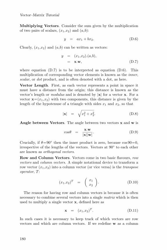
Multiplying Vectors. Consider the sum given by the multiplicationof two pairs of scalars, (x1,x2) and (a,b):

y = ax1 + bx2. (D.6)

Clearly, (x1,x2) and (a,b) can be written as vectors:

y = (x1,x2).(a,b),

= x.w, (D.7)

where equation (D.7) is to be interpreted as equation (D.6). Thismultiplication of corresponding vector elements is known as the inner,scalar, or dot product, and is often denoted with a dot, as here.

Vector Length. First, as each vector represents a point in space itmust have a distance from the origin; this distance is known as thevector’s length or modulus and is denoted by |x| for a vector x. For avector x=(x1,x2) with two components, this distance is given by thelength of the hypotenuse of a triangle with sides x1 and x2, so that

|x| =qx21 + x2

2. (D.8)

Angle between Vectors. The angle between two vectors x and w is

cos✓ =x.w

|x||w| . (D.9)

Crucially, if ✓=90� then the inner product is zero, because cos 90=0,irrespective of the lengths of the vectors. Vectors at 90� to each otherare known as orthogonal vectors.

Row and Column Vectors. Vectors come in two basic flavours, rowvectors and column vectors. A simple notational device to transform arow vector (x1,x2) into a column vector (or vice versa) is the transposeoperator, T :

(x1,x2)T =

✓x1

x2

◆. (D.10)

The reason for having row and column vectors is because it is oftennecessary to combine several vectors into a single matrix which is thenused to multiply a single vector x, defined here as

x = (x1,x2)T . (D.11)

In such cases it is necessary to keep track of which vectors are rowvectors and which are column vectors. If we redefine w as a column

180


vector, w=(a,b)T , then the inner product w.x can be written as

y = wTx (D.12)

= (a,b)

✓x1

x2

◆(D.13)

= ax1 + bx2. (D.14)

Here, each element of the row vector wT is multiplied by thecorresponding element of the column x, and the results are summed.Writing the inner product in this way allows us to specify many pairsof such products as a vector–matrix product.

If x is a vector variable such that x1 and x2 have been measured ntimes (e.g. at n time consecutive time steps) then y is a variable withn values

(y1,y2,...,yn) = (a,b)

✓x11, x12, ..., x1n

x21, x22, ..., x2n

◆. (D.15)

Here, each (single element) column y1t is given by the inner product ofthe corresponding column in x with the row vector w. This can nowbe rewritten succinctly as

y = wTx.

Vector–Matrix Multiplication. If we reset the number of times xhas been measured to N=1 for now then we can consider the simplecase of how two scalar values y1 and y2 are given by the inner products

y1 = wT1 x (D.16)

y2 = wT2 x, (D.17)

where w1=(a,b)T and w2=(c,d)T . If we consider the pair of values y1and y2 as a vector y=(y1,y2)T then we can rewrite equations (D.16)and (D.17) as

(y1,y2)T = (wT

1 x,wT2 x)

T . (D.18)

If we combine the column vectors w1 and w2 then we can define amatrix W :

W = (w1,w2)T (D.19)

=

✓a bc d

◆. (D.20)

181


We can now rewrite equation (D.18) as

(y1,y2)T =

✓a bc d

◆(x1,x2)

T . (D.21)

This can be written more succinctly as y=Wx. This defines thestandard syntax for vector–matrix multiplication. Note that thecolumn vector (x1,x2)T is multiplied by the first row in W to obtainy1 and is multiplied by the second row in W to obtain y2.

Just as the vector x represents a point on a plane, so the point yrepresents a (usually di↵erent) point on the plane. Thus the matrix Wimplements a linear geometric transformation of points from x to y.

If n>1 then the tth column (y1t,y2t)T in y is obtained as the productof the tth column (x1t,x2t)T in x with the row vectors in W :

✓y11, y12, ..., y1ny21, y22, ..., y2n

◆=

✓a bc d

◆✓x11, x12, ..., x1n

x21, x22, ..., x2n

◆

= (w1,w2)T (x1,x2)

T (D.22)

= Wx. (D.23)

Each (single element) column in y1 is a scalar value which is obtainedby taking the inner product of the corresponding column in x with thefirst row vector wT

1 in W . Similarly, each column in y2 is obtained bytaking the inner product of the corresponding column in x with thesecond row vector wT

2 in W .

Transpose of Vector–Matrix Product. It is useful to note that ify=Wx then the transpose yT of this vector–matrix product is

yT =(Wx)T =xTWT , (D.24)

where the transpose of a matrix is defined by

WT =

✓a bc d

◆T

=

✓a cb d

◆. (D.25)

Matrix Inverse. By analogy with scalar algebra, if y=Wx thenx=W�1y, where W�1 is the inverse of W . If the columns of a matrixare orthogonal then W�1=WT .

This tutorial is copied from Independent Component Analysis (2004),with permission from MIT Press.

182

Appendix E

Neural Information Methods

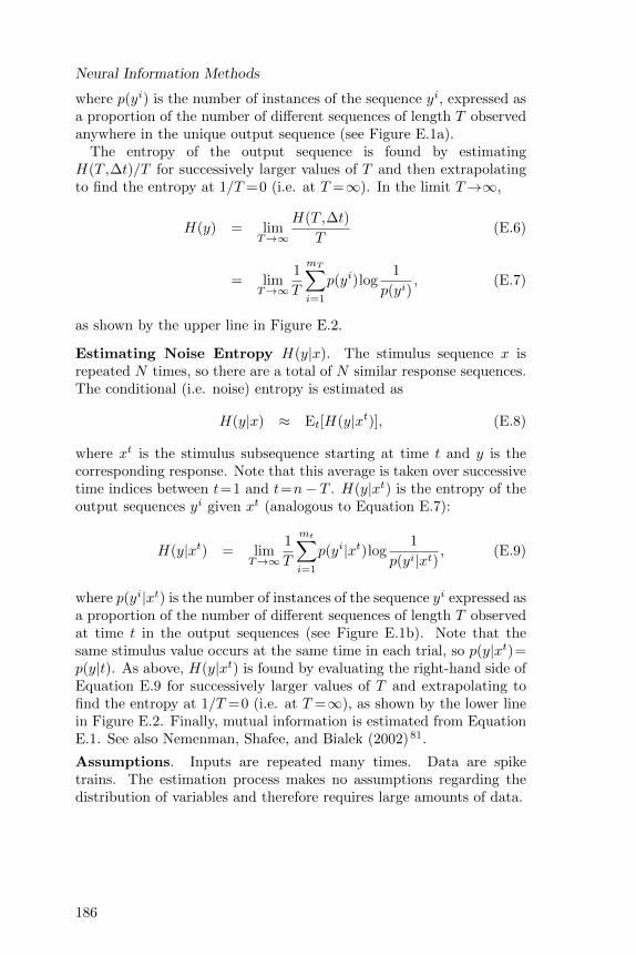
Consider a temporal sequence of stimulus values x and the resultantneuron outputs y, which can be either a sequence of continuous valuesor a sequence of spikes. The mutual information between x and y isdefined as

I(x,y) = H(y)�H(y|x) (E.1)

= H(x)�H(x|y) (E.2)

0.5 log(1 + SNR) bits, (E.3)

where SNR is the signal-to-noise ratio, with equality if each variable isindependent and Gaussian. The mutual information can be estimatedusing three broad strategies22, which provide: (1) a direct estimateusing Equation E.1, (2) an upper bound using Equation E.3, and (3) alower bound using Equation E.2. For simplicity, stimulus values (s inthe main text) are represented as x here, so that y=g(x) + ⌘, where gis a neuron transfer function and ⌘ is a noise term.

The Direct Method

The total entropy H(y) is essentially a global measure of how muchthe response sequence varies over time. In contrast, the noise entropyH(y|x) is a measure of how much variation in the response sequenceremains after the stimulus value at each point in time has been takeninto account. Therefore, the di↵erence between H(y) and H(y|x) is ameasure of the amount of variation in the response sequence that canbe attributed to the stimulus sequence.

Estimating the Entropy of a Spike Train. In physics, the entropyof a jar of gas is proportional to the volume of the jar. By analogy, wecan treat a spike train as if it were a one-dimensional jar, so that spiketrain entropy is proportional to the amount of time T over which thespike train is measured: H(T ,�t)/T , where �t defines the temporal

183


resolution used to measure spikes. Dividing H(T ,�t) by T yields theentropy rate, which converges to the entropy H(y) for large values ofT ; specifically,

H(y) = limT!1

H(T ,�t)

Tbits/s. (E.4)

Strong et al. (1998)118 use arguments from statistical mechanics toshow that a graph of H(T ,�t)/T versus 1/T should yield a straightline (see also Appendix A.8 in Bialek, 201218). The x-intercept of this

Trial SpikeTrains1 001000010111100011012 011000100011100010013 011000100011000010014 011000100001000010015 011000100001000010116 011000100001000010017 001000100001000111018 111000100001000010019 0100001010010000000110 01100010000100011001

Trial SpikeTrains 1 001000010111100011012 011000100011100010013 011000100011000010014 011000100001000010015 011000100001000010116 011000100001000010017 001000100001000111018 111000100001000010019 0100001010010000000110 01100010000100011001

(a) (b)

S:mulussequence S:mulussequence

35

Figure E.1. The direct method (schematic). The same stimulus sequence isrepeated for N=10 trials and the N response sequences are recorded; a spikeis represented as 1 and no spike as 0.(a) Total entropy H(y) is estimated from the probability of particular spiketrains within a long unique spike train sequence (which is the concatenationof 10 trials here). The probability p(y) of a particular T -element spike trainy is estimated as the number of instances of y expressed as a proportion of allT -element spike trains. For example, in the data above, there are 170 placeswhere a three-element spike train could occur, and there are 35 instances ofthe spike sequence y=[100] (marked in bold), so p(y)=35/170⇡0.206.(b) Noise entropy H(y|x) is estimated from the conditional probability ofparticular spike trains. The same stimulus value occurs at the same timein each of N=10 trials. Therefore, the conditional probability p(y|x) of theresponse y to a stimulus subsequence x which starts at time t is the numberNy of trials which contain y at time t expressed as a proportion of the numberN of spike trains that begin at time t (i.e. p(y|x)=p(y|t)). For example, thereare Ny=9 instances of the spike sequence y=[100] at t=3 (marked in bold),so the conditional probability is p(y=[100]|t=3)=9/10=0.9.

184


line is at 1/T = 0, corresponding to a y-intercept of H(T ,�t)/T atT =1, which is therefore the entropy H(y).

The direct method usually involves two types of output sequences:unique and repeated. The unique spike train is a response to a longsequence of inputs; this is used to estimate the total spike train entropy.The repeated spike train sequence consists of spike trains obtained inresponse to N repeats of a stimulus sequence; these are used to estimatethe entropy of the noise in the spike train. However, if the repeatedsequence is su�ciently long then the entire set of N response sequencescan be treated as a unique spike train, as in Figure E.1.

Estimating Total Entropy H(y). The entropy H(T ,�t) for onevalue of T is estimated from the probability p(yi) of the mT di↵erentobserved sequences y1,...,ymT of length T :

H(T ,�t) =m

TX

i=1

p(yi)log1

p(yi), (E.5)

4.3 Entropy and Information for Spike Trains 27

00

20 40 60 80 100

40

80

120

160

200

Figure 4.7: Entropy and noise entropy rates for the H1 visual neuron in the flyresponding to a randomly moving visual image. The filled circles in the uppertrace show the full spike-train entropy rate computed for different values of 1/Ts.The straight line is a linear extrapolation to 1/Ts = 0, which corresponds to Ts→∞. The lower trace shows the spike train noise entropy rate for different valuesof 1/Ts. The straight line is again an extrapolation to 1/Ts = 0. Both entropy ratesincrease as functions of 1/Ts , and the true spike-train and noise entropy rates areoverestimated at large values of 1/Ts. At 1/Ts ≈ 20/s, there is a sudden shift inthe dependence. This occurs when there is insufficient data to compute the spikesequence probabilities. The difference between the y intercepts of the two straightlines plotted is the mutual information rate. The resolution is!t= 3 ms. (Adaptedfrom Strong et al., 1998.)

stimuli in equation 4.6. The result is

hnoise = −!tT!

t

"

1Ts!

BP[B(t)] log2 P[B(t)]

#

(4.58)

where T/!t is the number of different t values being summed.

If equation 4.58 is based on finite-length spike sequences, it provides anupper bound on the noise entropy rate. The true noise entropy rate is es-timated by performing a linear extrapolation in 1/Ts to 1/Ts = 0, as wasdone for the spike-train entropy rate. This is done for the H1 data in figure4.7. The result is a noise entropy of 79 bits/s for !t = 3 ms. The infor-mation rate is obtained by taking the difference between the extrapolatedvalues for the spike-train and noise entropy rates. The result for the fly H1neuron used in figure 4.7, is an information rate of 157 - 79 = 78 bits/s or1.8 bits/spike. Values in the range 1 to 3 bits/spike are typical results ofsuch calculations for a variety of preparations.

Draft: December 17, 2000 Theoretical Neuroscience

Figure E.2. The direct method. Entropy and noise entropy rates for a visualneuron (H1 in the fly), responding to a randomly moving visual image. Thefilled circles in the upper trace show the full spike-train entropy rate fordi↵erent values of 1/T (with �t=3ms). The straight line is an extrapolationto 1/T=0 (i.e. T!1) and yields H(y). The lower trace shows the spike-trainnoise entropy rate for di↵erent values of 1/T , and the straight line is againan extrapolation to 1/T=0 and yields H(y|x). The di↵erence between theordinate intercepts of the two straight lines is H(y)�H(y|x) and is thereforethe mutual information rate (Equation E.1). Reproduced with permissionfrom Strong et al. (1998)118.

185


where p(yi) is the number of instances of the sequence yi, expressed asa proportion of the number of di↵erent sequences of length T observedanywhere in the unique output sequence (see Figure E.1a).

The entropy of the output sequence is found by estimatingH(T ,�t)/T for successively larger values of T and then extrapolatingto find the entropy at 1/T =0 (i.e. at T =1). In the limit T!1,

H(y) = limT!1

H(T ,�t)

T(E.6)

= limT!1

1

T

mTX

i=1

p(yi)log1

p(yi), (E.7)

as shown by the upper line in Figure E.2.

Estimating Noise Entropy H(y|x). The stimulus sequence x isrepeated N times, so there are a total of N similar response sequences.The conditional (i.e. noise) entropy is estimated as

H(y|x) ⇡ Et[H(y|xt)], (E.8)

where xt is the stimulus subsequence starting at time t and y is thecorresponding response. Note that this average is taken over successivetime indices between t=1 and t=n� T . H(y|xt) is the entropy of theoutput sequences yi given xt (analogous to Equation E.7):

H(y|xt) = limT!1

1

T

mtX

i=1

p(yi|xt)log1

p(yi|xt), (E.9)

where p(yi|xt) is the number of instances of the sequence yi expressed asa proportion of the number of di↵erent sequences of length T observedat time t in the output sequences (see Figure E.1b). Note that thesame stimulus value occurs at the same time in each trial, so p(y|xt)=p(y|t). As above, H(y|xt) is found by evaluating the right-hand side ofEquation E.9 for successively larger values of T and extrapolating tofind the entropy at 1/T =0 (i.e. at T =1), as shown by the lower linein Figure E.2. Finally, mutual information is estimated from EquationE.1. See also Nemenman, Shafee, and Bialek (2002)81.

Assumptions. Inputs are repeated many times. Data are spiketrains. The estimation process makes no assumptions regarding thedistribution of variables and therefore requires large amounts of data.

186


The Upper Bound Method

If the noise ⌘ in the output y has an independent Gaussian distributionthen the mutual information between x and y is maximised providedx also has an independent Gaussian distribution. Thus, if the inputx is Gaussian and independent then the estimated mutual informationprovides an upper bound. Additionally, if each variable is Gaussian(but not necessarily independent) with a bandwidth of W Hz then itsentropy is the sum of the entropies of its Fourier components. To reviewFourier analysis, see Sections 2.8 and 7.4.

In common with the direct method, input sequences need to berepeated many times, but the number N of trials (repeats) requiredhere is fewer. This is because a Gaussian distribution is defined interms of its mean and variance, so, in e↵ect, we only need to estimatea few means and variances from the data.

Estimating Output Signal Power

1. Find the average output sequence y=1/NPN

i=1yi.

2. Obtain Fourier coe�cient (a(f),b(f)) of y at each frequency f .

3. Estimate the power of each frequency f as S(f)=a(f)2 + b(f)2.

Estimating Output Noise Power

1. Estimate the noise ⌘i=yi � y in each of the N output sequences.

2. Find the Fourier coe�cient (a(f),b(f)) of ⌘i at each frequency f .

3. Estimate the power at each frequency f as N i(f)=a(f)2+ b(f)2.

4. Find the average power of each Fourier component

N (f) =1

N

NX

i=1

N i(f). (E.10)

Assuming a Nyquist sampling rate of 2W Hz, estimate the mutualinformation I(x,y) by summing over frequencies (as in Equation 2.28):

Rinfo =WX

f=0

log

✓1 +

S(f)N (f)

◆bits/s, (E.11)

where Rinfo � I(x,y), with equality if each variable is iid Gaussian.

Assumptions. The response sequences to each of N repeats of thesame stimulus sequence are continuous. Each output sequence isGaussian, but not necessarily independent (iid).

187


The Lower Bound Method

Unlike previous methods, this method does not rely on repeatedpresentations of the same stimulus, and it can be used for spikingor continuous outputs. In both cases, we can use the neuron inputsx and outputs y to estimate a linear decoding filter wd. When theoutput sequence is convolved with this filter, it provides an estimatexest=wd⌦y of the stimulus x, where ⌦ is the convolution operator. Weassume that x=xest+⇠est, so that the estimated noise in the estimatedstimulus sequence is ⇠est=x� xest (Figure 1.3).

Assuming a bandwidth of W Hz and that values are transmittedat the Nyquist rate of 2W Hz, we Fourier transform the stimulussequence x to find the signal power X (f) at each frequency f andFourier transform ⇠est to find the power in the estimated noise M(f)at each frequency. The mutual information is estimated by summingover frequencies:

Rmin = H(x)�H(⇠est) (E.12)

=X

f

logX (f)�X

f

logM(f) (E.13)

=WX

f=0

logX (f)

M(f)bits/s, (E.14)

where RminI(x,y), with equality if each variable is iid Gaussian.

Assumptions. The stimulus sequence x is Gaussian, but notnecessarily independent (iid). Outputs are spiking or continuous.

Further Reading. This account is based on Strong et al. (1998)118,Rieke et al. (1997)98, Borst and Theunissen (1999)22, Dayan and Abbot(2001)33, and Niven et al. (2007)83. Relevant developments can befound in Nemenman, Shafee, and Bialek (2002)81, Juusola et al. (2003,2016)57;58, Ince et al. (2009)53, Goldberg et al. (2009)48, Crumiller etal. (2013)31, Valiant and Valiant (2013)119, and Dettner et al. (2016)35.

188

Appendix F

Key EquationsLogarithms use base 2 unless stated otherwise.

Entropy

H(s) =mX

i=1

p(xi) log1

p(xi)bits (F.1)

H(s) =

Z

x

p(x) log1

p(x)dx bits (F.2)

Joint Entropy

H(x,y) =mX

i=1

mX

j=1

p(xi,yj) log1

p(xi,yj)bits (F.3)

H(x,y) =

Z

y

Z

x

p(x,y) log1

p(x,y)dx dy bits (F.4)

H(x,y) = I(x,y) +H(x|y) +H(y|x) bits (F.5)

Conditional Entropy

H(y|s) =mX

i=1

mX

j=1

p(xi,yj) log1

p(xi|yj)bits (F.6)

H(y|x) =mX

i=1

mX

j=1

p(xi,yj) log1

p(yj |xi)bits (F.7)

H(x|y) =

Z

y

Z

x

p(x,y) log1

p(x|y) dx dy bits (F.8)

H(y|x) =

Z

y

Z

x

p(x,y) log1

p(y|x) dx dy bits (F.9)

H(x|y) = H(x,y)�H(y) bits (F.10)

H(y|x) = H(x,y)�H(x) bits, (F.11)

189

Key Equations

from which we obtain the chain rule for entropy:

H(x,y) = H(x) +H(y|x) bits (F.12)

= H(y) +H(x|y) bits (F.13)Marginalisation

p(xi) =mX

j=1

p(xi,yj), p(yj) =mX

i=1

p(xi,yj) (F.14)

p(x) =

Z

y

p(x,y) dy, p(y) =

Z

x

p(x,y) dx (F.15)

Mutual Information

I(x,y) =mX

i=1

mX

j=1

p(xi,yj) logp(xi,yj)

p(xi)p(yj)bits (F.16)

I(x,y) =

Z

y

Z

x

p(x,y) logp(x,y)

p(x)p(y)dx dy bits (F.17)

I(x,y) = H(x) +H(y)�H(x,y) (F.18)

= H(x)�H(x|y) (F.19)

= H(y)�H(y|x) (F.20)

= H(x,y)� [H(x|y) +H(y|x)] bits (F.21)

If y=x+ ⌘, with x and y (not necessarily iid) Gaussian variables, then

I(x,y) =

Z W

f=0log

✓1 +

S(f)

N(f)

◆df bits/s, (F.22)

where W is the bandwidth, S(f)/N(f) is the signal-to-noise ratio ofthe signal and noise Fourier components at frequency f (Section 2.8),and data are transmitted at the Nyquist rate of 2W samples/s.

Channel Capacity

C = maxp(x)

I(x,y) bits per value. (F.23)

If the channel input x has variance S, the noise ⌘ has variance N , andboth x and ⌘ are iid Gaussian variables then I(x,y)=C, where

C =1

2log

✓1 +

S

N

◆bits per value, (F.24)

where the ratio of variances S/N is the signal-to-noise ratio.

190

References[1] Adelson, EH and Bergen, JR. Spatiotemporal energy models for the

perception of motion. J Optical Society of America A, 2(2):284–299,1985.

[2] Adrian, ED. The impulses produced by sensory nerve endings: Part I.J Physiology, 61:49–72, 1926.

[3] Alexander, RM. Optima for Animals. Princeton University Press, 1996.[4] Atick, JJ. Could information theory provide an ecological theory

of sensory processing? Network: Computation in Neural Systems,3(2):213–251, 1992.

[5] Atick, JJ, Li, Z, and Redlich, AN. Understanding retinal color codingfrom first principles. Neural Computation, 4(4):559–572, 1992.

[6] Atick, JJ and Redlich, AN. Towards a theory of early visual processing.Neural Computation, 2(3):308–320, 1990.

[7] Atick, JJ and Redlich, AN. What does the retina know about naturalscenes? Neural Computation, 4(2):196–210, 1992.

[8] Attneave, F. Some informational aspects of visual perception.Psychological Review, pages 183–193, 1954.

[9] Attwell, D and Laughlin, SB. An energy budget for signaling in thegrey matter of the brain. J Cerebral Blood Flow and Metabolism,21(10):1133–1145, 2001.

[10] Baddeley, R, Abbott, LF, Booth, MCA, Sengpiel, F, Freeman, T,Wakeman, EA, and Rolls, ET. Responses of neurons in primary andinferior temporal visual cortices to natural scenes. Proc Royal SocietyLondon B, 264:1775–1783, 1997.

[11] Bair, W. Analysis of Temporal Structure in Spike Trains of VisualCortical Area MT. PhD thesis, California Institute of Technology, 1996.

[12] Balasubramanian, V. Heterogeneity and e�ciency in the brain. ProcIEEE, 103(8):1346–1358, 2015.

[13] Balasubramanian, V and Sterling, P. Receptive fields and functionalarchitecture in the retina. J Physiology, 587(12):2753–2767, 2009.

[14] Barlow, HB. Sensory mechanisms, the reduction of redundancy, andintelligence. In Blake, DV and Utlley, AM, editors, Proc SympMechanisation of Thought Processes, Vol 2. HM Stationery O�ce,1959.

[15] Barlow, HB. Possible principles underlying the transformations ofsensory messages. Sensory Communication, pages 217–234, 1961.

[16] Barlow, HB, Fitzhugh, R, and Ku✏er, SW. Change of organizationin the receptive fields of the cat’s retina during dark adaptation. JPhysiology, 137:338–354, 1957.

[17] Bell, AJ and Sejnowski, TJ. An information-maximization approach toblind separation and blind deconvolution. Neural Computation, 7:1129–1159, 1995.

[18] Bialek, W. Biophysics: Searching for Principles. Princeton UniversityPress, 2012.

191

References

[19] Bialek, W, DeWeese, M, Rieke, F, and Warland, D. Bits andbrains: Information flow in the nervous system. Physica A: StatisticalMechanics and its Applications, 200(1–4):581–593, 1993.

[20] Bogacz, R. A tutorial on the free-energy framework for modellingperception and learning. J Mathematical Psychology, 2015.

[21] Borghuis, BG, Ratli↵, CP, Smith, RG, Sterling, P, and Balasubrama-nian, V. Design of a neuronal array. J Neuroscience, 28(12):3178–3189,2008.

[22] Borst, A and Theunissen, FE. Information theory and neural coding.Nature Neuroscience, 2(11):947–957, 1999.

[23] Brainard, DH, Longere, P, Delahunt, PB, Freeman, WT, Kraft, JM,and Xiao, B. Bayesian model of human color constancy. J Vision,6(11), 2006.

[24] Brendel, W, Bourdoukan, R, Vertechi, P, Machens, CK, and Deneve,S. Learning to represent signals spike by spike, 2017. arXiv:1703.03777.

[25] Brenner, N, Bialek, W, and de Ruyter van Steveninck, R. Adaptiverescaling maximizes information transmission. Neuron, 26:695–702,2000.

[26] Brenner, N, Strong, SP, Koberle, R, Bialek, W, and de Ruyter vanSteveninck, RR. Synergy in a neural code. Neural Computation,12(7):1531–1552, 2000.

[27] Buchsbaum, G and Gottschalk. Trichromacy, opponent colours codingand optimum colour information transmission in the retina. Proc RoyalSociety London B, 220(1218):89–113, 1983.

[28] Chalk, M, Marre, O, and Tkacik, G. Toward a unified theory ofe�cient, predictive, and sparse coding. Proc National Academy ofSciences USA, 115(1):186–191, 2018.

[29] Charnov, EL. Optimal foraging, the marginal value theorem.Theoretical Population Biology, 9(2):129–136, 1976.

[30] Cover, TM and Thomas, JA. Elements of Information Theory. NewYork, John Wiley and Sons, 1991.

[31] Crumiller, M, Knight, B, and Kaplan, E. The measurement ofinformation transmitted by a neural population: Promises andchallenges. Entropy, 15(9):3507–3527, 2013.

[32] Davies, NB, Krebs, JR, and West, SA. An Introduction to BehaviouralEcology. Wiley, 2012.

[33] Dayan, P and Abbott, LF. Theoretical Neuroscience. MIT Press, NewYork, NY, USA, 2001.

[34] de Ruyter van Steveninck, RR and Laughlin, SB. The rateof information transfer at graded-potential synapses. Nature,379(6566):642, 1996.

[35] Dettner, A, Munzberg, S, and Tchumatchenko, T. Temporal pairwisespike correlations fully capture single-neuron information. NatureCommunications, 7, 2016.

[36] DeWeese, MR. Optimization Principles for the Neural Code. PhDthesis, Princeton University, 1995.

[37] DeWeese, MR and Bialek, W. Information flow in sensory neurons. IlNuovo Cimento D, 17(7-8):733–741, 1995.

[38] Doi, E, Gauthier, JL, Field, GD, Shlens, J, Sher, A, Greschner,M, Machado, TA, Jepson, LH, Mathieson, K, Gunning, DE, Litke,AM, Paninski, L, Chichilnisky, EJ, and Simoncelli, EP. E�cientcoding of spatial information in the primate retina. J Neuroscience,32(46):16256–16264, 2012.

192

References

[39] Du↵y, KR and Hubel, DH. Receptive field properties of neurons in theprimary visual cortex under photopic and scotopic lighting conditions.Vision Research, 47:2569–2574, 2007.

[40] Eliasmith, C and Anderson, CH. Neural Engineering. MIT Press, 2004.[41] Fairhall, AL, Lewen, GD, Bialek, W, and de Ruyter van Steveninck,

RR. E�ciency and ambiguity in an adaptive neural code. Nature,412(6849):787–792, 2001.

[42] Faisal, AA and Laughlin, SB. Stochastic simulations on the reliabilityof action potential propagation in thin axons. PLoS Comp Biol,3(5):e79, 2007.

[43] Finelli, LA, Haney, S, Bazhenov, M, Stopfer, M, and Sejnowski, TJ.Synaptic learning rules and sparse coding in a model sensory system.PLoS Comp Biology, 4(4), 2008.

[44] Foldiak, P and Young, M. Sparse coding in the primate cortex. InArbib, MA (ed.), The Handbook of Brain Theory and Neural Networks,pages 895–898, 1995.

[45] Frisby, JP and Stone, JV. Seeing: The Computational Approach toBiological Vision. MIT Press, 2010.

[46] Gaudry, Kate S and Reinagel, Pamela. Benefits of contrastnormalization demonstrated in neurons and model cells. JNeuroscience, 27(30):8071–8079, 2007.

[47] Gerstner, W and Kistler, WM. Spiking Neuron Models: SingleNeurons, Populations, Plasticity. CUP, 2002.

[48] Goldberg, David H, Victor, Jonathan D, Gardner, Esther P, andGardner, Daniel. Spike train analysis toolkit: enabling widerapplication of information-theoretic techniques to neurophysiology.Neuroinformatics, 7(3):165–178, 2009.

[49] Guo, D, Shamai, S, and Verdu, S. Mutual information and minimummean-square error in Gaussian channels. IEEE Transactions onInformation Theory, 51(4):1261–1282, 2005.

[50] Harris, JJ, Jolivet, R, Engl, E, and Attwell, D. Energy-e�cientinformation transfer by visual pathway synapses. Current Biology,25(24):3151–3160, 2015.

[51] Hartline, HK. Visual receptors and retinal interaction, 1967. NobelLecture.

[52] Hosoya, T, Baccus, SA, and Meister, M. Dynamic predictive codingby the retina. Nature, 436(7047):71–77, 2005.

[53] Ince, RAA, Petersen, RS, Swan, DC, and Panzeri, S. Pythonfor information theoretic analysis of neural data. Frontiers inNeuroinformatics, 3, 2009.

[54] Jacobs, A L, Fridman, G, Douglas, RM, Alam, NM, Latham, PE,Prusky, GT, and Nirenberg, S. Ruling out and ruling in neural codes.Proc National Academy of Sciences USA, 106(14):5936–5941, 2009.

[55] Jarvstad, A, Rushton, SK, Warren, PA, and Hahn, U. Knowing whento move on cognitive and perceptual decisions in time. PsychologicalScience, 23(6):589–597, 2012.

[56] Johnson, EC, Jones, DL, and Ratnam, R. A minimum-error, energy-constrained neural code is an instantaneous-rate code. J ComputationalNeuroscience, 40(2):193–206, 2016.

[57] Juusola, M, Dau, A, and Lei Z, Diana R. Electrophysiologicalmethod for recording intracellular voltage responses of Drosophilaphotoreceptors and interneurons to light stimuli in vivo. JoVE, (112),2016.

[58] Juusola, M and de Polavieja, GG. The rate of information transferof naturalistic stimulation by graded potentials. J General Physiology,

193

References

122(2):191–206, 2003.[59] Koch, K, McLean, J, Berry, M, Sterling, P, Balasubramanian, V, and

Freed, MA. E�ciency of information transmission by retinal ganglioncells. Current Biology, 14(17):1523 – 1530, 2004.

[60] Koch, K, McLean, J, Segev, R, Freed, MA, Berry, MJ,Balasubramanian, V, and Sterling, P. How much the eye tells thebrain. Current Biology, 16(14):1428–1434, 07 2006.

[61] Kostal, L, Lansky, P, and Rospars, J-P. E�cient olfactory coding inthe pheromone receptor neuron of a moth. PLoS Comp Biol, 4(4),2008.

[62] Ku✏er, SW. Discharge patterns and functional organization ofmammalian retina. J Neurophysiology, 16:37–68, 1953.

[63] Land, MF and Nilsson, DE. Animal Eyes. OUP, 2002.[64] Laughlin, SB. A simple coding procedure enhances a neuron’s

information capacity. Z Naturforsch, 36c:910–912, 1981.[65] Laughlin, SB. Matching coding to scenes to enhance e�ciency. In

Braddick, OJ and Sleigh, AC (eds), Physical and Biological Processingof Images, pages 42–52. Springer, Berlin, 1983.

[66] Laughlin, SB. Form and function in retinal processing. Trends inNeurosciences, 10:478–483, 1987.

[67] Laughlin, SB, de Ruyter van Steveninck, RR, and Anderson, JC. Themetabolic cost of neural information. Nature Neuroscience, 1(1):36–41,1998.

[68] Laughlin, SB, Howard, J, and Blakeslee, B. Synaptic limitations tocontrast coding in the retina of the blowfly Calliphora. Proc RoyalSociety London B, 231(1265):437–467, 1987.

[69] Lennie, P. The cost of cortical computation. Current Biology, 13:493–497, 2003.

[70] Levy, WB and Baxter, RA. Energy e�cient neural codes. NeuralComputation, 8(3):531–543, 1996.

[71] Linsker, R. Self-organization in perceptual network. Computer, pages105–117, 1988.

[72] Liu, P and Cheng, B. Limitations of rotational manoeuvrabilityin insects and hummingbirds: evaluating the e↵ects of neuro-biomechanical delays and muscle mechanical power. J Royal SocietyInterface, 14(132):20170068, 2017.

[73] Liu, Y, Yue, Y, Yu, Y, Liu, L, and Yu, L. E↵ects of channel blockingon information transmission and energy e�ciency in squid giant axons.J Computational Neuroscience, 44(2):219–231, 2018.

[74] London, M, Roth, A, Beeren, L, Hausser, M, and Latham, PE.Sensitivity to perturbations in vivo implies high noise and suggestsrate coding in cortex. Nature, 466(7302):123, 2010.

[75] MacKay, DM and McCulloch, WS. The limiting information capacityof a neuronal link. Bull. Mathematical Biophysics, 14(2):127–135, 1952.

[76] Mainen, ZF and Sejnowski, TJ. Reliability of spike timing inneocortical neurons. Science, 268(5216):1503, 1995.

[77] Marr, D. Vision: A Computational Investigation into the HumanRepresentation and Processing of Visual Information. MIT Press, 2010.Originally published by W.H. Freeman, 1982.

[78] Mather, G. Foundations of Perception. Taylor and Francis, 2006.[79] Meister, M and Berry, MJ. The neural code of the retina. Neuron,

22:435–450, 1999.[80] Moujahid, A, D’Anjou, A, and Grana, M. Energy demands of diverse

spiking cells from the neocortex, hippocampus, and thalamus. Frontiers

194

References

in Computational Neuroscience, 8:41, 2014.[81] Nemenman, I, Shafee, F, and Bialek, W. Entropy and inference,

revisited. In Dietterich, TG, Becker, S, and Ghahramani, Z (eds),Advances in Neural Information Processing Systems 14. MIT Press,2002.

[82] Nirenberg, S, Carcieri, SM, Jacobs, AL, and Latham, PE. Retinalganglion cells act largely as independent encoders. Nature,411(6838):698–701, June 2001.

[83] Niven, JE, Anderson, JC, and Laughlin, SB. Fly photoreceptorsdemonstrate energy-information trade-o↵s in neural coding. PLoSBiology, 5(4), 03 2007.

[84] Nyquist, H. Certain topics in telegraph transmission theory. ProcIEEE, 90(2):280–305, 1928.

[85] Oja, E. Oja learning rule. Scholarpedia, 3(3):3612, 2008.[86] Pajevic, S and Basser, PJ. An optimum principle predicts the

distribution of axon diameters in white matter. PLoS ONE, 8(1), 2013.[87] Park, M and Pillow, JW. Bayesian e�cient coding, 2017.

bioRxiv:178418.[88] Perge, JA, Koch, K, Miller, R, Sterling, P, and Balasubramanian, V.

How the optic nerve allocates space, energy capacity, and information.J Neuroscience, 29(24):7917–7928, 2009.

[89] Perge, JA, Niven, JE, Mugnaini, E, Balasubramanian, V, and Sterling,P. Why do axons di↵er in caliber? J Neuroscience, 32(2):626–638,2012.

[90] Persi, E, Hansel, D, Nowak, L, Barone, P, and van Vreeswijk, C. Power-law input-output transfer functions explain the contrast-response andtuning properties of neurons in visual cortex. PLoS Comp Biol,7(2):e1001078, 02 2011.

[91] Pitkow, X and Meister, M. Decorrelation and e�cient coding by retinalganglion cells. Nature Neuroscience, 15(4):628–635, 04 2012.

[92] Plumbley, MD. E�cient information transfer and anti-Hebbian neuralnetworks. Neural Networks, 6:823–833, 1993.

[93] Plumbley, MD and Fallside, F. The e↵ect of receptor signal-to-noiselevels on optimal filtering in a sensory system. In Acoustics, Speech,and Signal Processing (ICASSP) 1991, pages 2321–2324. IEEE, 1991.

[94] Rajan, K and Bialek, W. Maximally informative ‘stimulus energies’in the analysis of neural responses to natural signals. PLoS ONE,8(11):e71959, 2013.

[95] Rao, RPN and Ballard, DH. Predictive coding in the visual cortex: afunctional interpretation of some extra-classical receptive-field e↵ects.Nature Neuroscience, 2:79–87, 1999.

[96] Reza, FM. Information Theory. New York, McGraw-Hill, 1961.[97] Rieke, F, Bodnar, DA, and Bialek, W. Naturalistic stimuli increase

the rate and e�ciency of information transmission by primary auditorya↵erents. Proc Royal Society London B, 262(1365):259–265, 1995.

[98] Rieke, F, Warland, D, de Ruyter van Steveninck, RR, and Bialek, W.Spikes: Exploring the Neural Code. MIT Press, Cambridge, MA, 1997.

[99] Riley, KF, Hobson, MP, and Bence, SJ. Mathematical Methods forPhysics and Engineering. Cambridge University Press, 2006.

[100] Ruderman DL, Cronin, TW and Chiao, C. Statistics of cone responsesto natural images: implications for visual coding. J Optical Society ofAmerica, 15:2036–2045, 1998.

[101] Saul, AB and Humphrey, AL. Spatial and temporal response propertiesof lagged and nonlagged cells in cat lateral geniculate nucleus. J

195

References

Neurophysiology, 64(1):206–224, 1990.[102] Schultz, SR. Signal-to-noise ratio in neuroscience. Scholarpedia,

2(6):2046, 2007.[103] Sengupta, B, Stemmler, MB, and Friston, KJ. Information and

e�ciency in the nervous system – a synthesis. PLoS Comp Biol, 2013.[104] Shannon, CE. A mathematical theory of communication. Bell System

Technical Journal, 27:379–423, 1948.[105] Shannon, CE and Weaver, W. The Mathematical Theory of

Communication. University of Illinois Press, 1949.[106] Sharpee, T, Rust, NC, and Bialek, W. Analyzing neural responses

to natural signals: maximally informative dimensions. NeuralComputation, 16(2):223–250, 2004.

[107] Sharpee, TO. Computational identification of receptive fields. Annualreview of neuroscience, 36:103–120, 2013.

[108] Smith, EC and Lewicki, MS. E�cient auditory coding. Nature,439(7079):978–982, 2006.

[109] Smith, S. The Scientist and Engineer’s Guide to Digital SignalProcessing. 1997. Freely available at www.dspguide.com.

[110] Sokolo↵, L. Circulation and energy metabolism of the brain. BasicNeurochemistry, 2:338–413, 1989.

[111] Solomon, SG and Lennie, P. The machinery of colour vision. NatureReviews Neuroscience, 8(4):276–286, 2007.

[112] Srinivasan, MV, Laughlin, SB, and Dubs, A. Predictive coding: afresh view of inhibition in the retina. Proc Royal Society London B,216(1205):427–459, 1982.

[113] Srinivasan, MV, Pinter, RB, and Osorio, D. Matched filtering in thevisual system. Proc Royal Society London B, 240(1298):279–293, 1990.

[114] Sterling, P and Laughlin, S. Principles of Neural Design. MIT Press,2015.

[115] Stone, JV. Independent Component Analysis: A Tutorial Introduction.MIT Press, Boston, 2004.

[116] Stone, JV. Vision and Brain. MIT Press, 2012.[117] Stone, JV. Information Theory: A Tutorial Introduction. Sebtel Press,

She�eld, England, 2015.[118] Strong, SP, Koberle, R, de Ruyter van Steveninck, RR, and Bialek,

W. Entropy and information in neural spike trains. Physical ReviewLetters, 80(1):197, 1998.

[119] Valiant, P and Valiant, G. Estimating the unseen: Improved estimatorsfor entropy and other properties. In Advances in Neural InformationProcessing Systems, pages 2157–2165, 2013.

[120] van Hateren, JH. Theoretical predictions of spatiotemporal receptivefields of fly LMCs, and experimental validation. J ComparativePhysiology A, 171(2):157–170, 1992.

[121] van Hateren, JH. A theory of maximizing sensory information.Biological Cybernetics, 68:23–29, 1992.

[122] van Hateren, JH. Processing of natural time series of intensities by thevisual system of the blowfly. Vision Research, 37(23):3407–3416, 1997.

[123] Vincent, BT and Baddeley, RJ. Synaptic energy e�ciency in retinalprocessing. Vision Research, 43(11):1285–1292, 2003.

[124] Wei, X and Stocker, AA. Mutual information, Fisher information, ande�cient coding. Neural Computation, 28(2):305–326, 2016.

[125] Zhaoping, L. Understanding Vision: Theory, Models, and Data. OUPOxford, 2014.

196

Index

action potential, 28adenosine triphosphate (ATP),

49, 169aftere↵ect, 63apposition eye, 150autocorrelation function, 106,

169automatic gain control, 155average, 169axon, 27axon diameter, 50

spike speed, 55

bandwidth, 24, 169binary

digits vs bits, 11bit, 10, 12, 169Bussgang’s theorem, 105

calculus of variations, 45, 54capacity, 17, 169, 190central limit theorem, 36, 162,

169channel capacity, 9, 17, 18chromatic aberration, 64coding capacity, 33, 43, 57, 169coding e�ciency, 3, 37, 38, 169colour aftere↵ect, 63communication channel, 9compound eye, 149conditional entropy, 21, 169conditional probability, 169conduction velocity, 28, 55cone, 64contrast, 123, 133, 154convolution operator, 100, 122

cornea, 149correlation, 169correlation coe�cient, 177correlation time, 42covariance, 73covariance matrix, 86, 107, 169Cramer-Rao bound, 95cricket, 39cross-correlation function, 105,

109, 170cumulative distribution func-

tion, 159, 161, 170

dark noise, 70data processing inequality, 22decoding, 170decorrelated, 170dendrite, 27determinant, 86die, 14di↵erence-of-Gaussian, 124di↵erential entropy, 23direct method, 37, 183dot product, 76, 100dynamic linearity, 92, 170dynamic range, 154

e�cient coding hypothesis, 4,50, 170

e�cient metabolic principle,165

encoding, 9entropy, 12, 13, 170, 189entropy rate, 35, 184entropy vs information, 15equiprobable, 170

197

Index

equivariant, 69, 170expected number, 32expected value, 170exponential decay, 29exponential distribution, 17, 57

filter, 42, 92, 170Gaussian, 124

firing rate, 28optimal, 57

fly’s eye, 149Fourier analysis, 24, 25, 120,

128, 170, 187, 190fovea, 64

Galileo, Galilei, 5ganglion cell, 65, 89, 110, 115,

122Gaussian

channel, 22distribution, 16, 36variable, 170

glial cell, 58

ideal observer model, 41identity matrix, 86, 170iid, 16, 170independence, 13, 170, 178information, 11, 14, 170information estimation, 183information theory, 6, 9information vs entropy, 15inner product, 76, 100

Joule, 43, 170

kernel, 93, 120, 170

large monopolar cell, 50, 150,153

least-squares estimate, 95linear, 170

decodability, 42, 171filter, 37, 92, 112, 142function, 97superposition, 93, 97

system, 93time invariant, 93

linear decodability, 171linearity

dynamic, 92static, 92

LMC, 50, 150, 153LNP neuron model, 99log-normal, 159logarithm, 11, 12, 171low-pass filter, 120lower bound method, 37, 188

marginal value theorem, 44marginalisation, 190Marr, David, 6matrix, 76, 181maximum entropy, 16maximum entropy e�ciency, 58maximum likelihood, 95measurement precision, 39metabolic e�ciency, 44, 53, 171Mexican hat, 123midget ganglion cell, 89mimic model, 93mitochondria, 48, 171mitochondrial volume, 51model

linear filter, 92mimic, 93predictive coding, 94

monotonic, 171mutual information, 21, 37,

171, 190Gaussian channel, 16

myelin sheath, 29, 49and spike speed, 55

natural statistics, 171neural superposition, 150, 151neuron, 2, 27noise, 6, 171noisy channel coding theorem,

21, 26

198

Index

o↵-centre cell, 123ommatidia, 149on-centre cell, 123opponent process, 67, 89, 124optic nerve, 2, 45, 47optical superposition, 150optimal foraging theory, 44orthogonal, 171

parasol ganglion cell, 89phase, 25, 171photoreceptor, 2, 64Poisson distribution, 36Poisson process, 31power, 23, 24, 171power spectrum, 25, 171predictive coding, 94, 96, 110,

141principal component analysis,

85, 171probability

density function, 16, 171distribution, 13, 171

pyramidal cell, 27, 58, 172

random variable, 12, 172rate code, 40receptive field, 65

on-centre, 123optimal size/spacing, 147

redundancy, 172redundancy reduction, 115retinal ganglion cell, 65reverse correlation, 101rhabdom, 149rhodopsin, 64rod, 64rotation matrix, 79

scalar variable, 76Shannon, Claude, 6, 9signal-to-noise ratio, 24, 172source coding theorem, 18space constant, 30spatial frequency, 120

spike, 2, 28cost, 49speed, 55timing precision, 39

spike-triggered average, 101static linearity, 92, 172synapse, 29system filter, 133

theorem, 9, 172timing code, 40timing precision, 39, 172transfer function, 29, 99, 100,

172transpose operator, 77, 180,

182tuning curve, 64tuning function, 172

uncertainty, 13, 14, 172uncorrelated, 172uniform distribution, 17, 153upper bound method, 37, 187

variable, 172scalar, 76vector, 75

vector, 75, 172, 179variable, 75

water-filling, 83, 135white spectrum, 129, 172Wiener kernel, 92, 100, 172

199

Dr James Stone is an Honorary Reader in Vision and ComputationalNeuroscience at the University of She�eld, England.

SeeingThe Computational Approach to Biological Vision

John P. Frisby and James V. Stone

second edition

Praise for Principles of Neural Information...

Documents

Transcript of Praise for Principles of Neural Information...