Pragmatic Electrical Engineering: Systems and Instruments
145
SYNTHESIS LECTURES ON DIGITAL CIRCUITS AND SYSTEMS C M & Morgan Claypool Publishers & Pragmatic Electrical Engineering Systems and Instruments William J. Eccles Mitchell Thornton, Series Editor
-
Upload
cory-fraser -
Category
Documents
-
view
128 -
download
6
description
By Morgan and Claypool
Transcript of Pragmatic Electrical Engineering: Systems and Instruments

Morgan Claypool Publishers&SYNTHESIS LECTURES ON
DIGITAL CIRCUITS AND SYSTEMSw w w . m o r g a n c l a y p o o l . c o m
MO
RG
AN
&C
LA
YP
OO
L
CM& Morgan Claypool Publishers&SYNTHESIS LECTURES ON
DIGITAL CIRCUITS AND SYSTEMS
Series Editor: Mitchell Thornton, Southern Methodist University
EC
CL
ES
PR
AG
MA
TIC
EL
EC
TR
ICA
L E
NG
INE
ER
ING
Pragmatic ElectricalEngineeringSystems and Instruments
William J. Eccles
Series ISSN: 1932-3166
Mitchell Thornton, Series Editor
About SYNTHESIsThis volume is a printed version of a work that appears in the Synthesis
Digital Library of Engineering and Computer Science. Synthesis Lectures
provide concise, original presentations of important research and development
topics, published quickly, in digital and print formats. For more information
visit www.morganclaypool.com
ISBN: 978-1-60845-671-0
9 781608 456710
90000
Pragmatic Electrical EngineeringSystems and Instruments
William J. Eccles, Rose-Hulman Institute of Technology
Pragmatic Electrical Engineering: Systems and Instruments is about some of the non-energy parts of
electrical systems, the parts that control things and measure physical parameters. The primary topics
are control systems and their characterization, instrumentation, signals, and electromagnetic
compatibility.
This text features a large number of completely worked examples to aid the reader in under-
standing how the various principles fit together.
While electric engineers may find this material useful as a review, engineers in other fields can
use this short lecture text as a modest introduction to these non-energy parts of electrical systems.
Some knowledge of basic d-c circuits and of phasors in the sinusoidal steady state is presumed.


Pragmatic Electrical Engineering:Systems and Instruments

Copyright © 2011 by Morgan & Claypool
All rights reserved. No part of this publication may be reproduced, stored in a retrieval system, or transmitted inany form or by any means—electronic, mechanical, photocopy, recording, or any other except for brief quotations inprinted reviews, without the prior permission of the publisher.
Pragmatic Electrical Engineering: Systems and Instruments
William Eccles
www.morganclaypool.com
ISBN: 9781608456710 paperbackISBN: 9781608456727 ebook
DOI 10.2200/S00353ED1V01Y201105DCS034
A Publication in the Morgan & Claypool Publishers seriesSYNTHESIS LECTURES ON DIGITAL CIRCUITS AND SYSTEMS
Lecture #34Series Editor: Mitchell A. Thornton, Southern Methodist University
Series ISSNSynthesis Lectures on Digital Circuits and SystemsPrint 1932-3166 Electronic 1932-3174

Synthesis Lectures on DigitalCircuits and Systems
EditorMitchell A. Thornton, Southern Methodist University
The Synthesis Lectures on Digital Circuits and Systems series is comprised of 50- to 100-page bookstargeted for audience members with a wide-ranging background. The Lectures include topics that areof interest to students, professionals, and researchers in the area of design and analysis of digital circuitsand systems. Each Lecture is self-contained and focuses on the background information required tounderstand the subject matter and practical case studies that illustrate applications. The format of aLecture is structured such that each will be devoted to a specific topic in digital circuits and systemsrather than a larger overview of several topics such as that found in a comprehensive handbook. TheLectures cover both well-established areas as well as newly developed or emerging material in digitalcircuits and systems design and analysis.
Pragmatic Electrical Engineering: Systems and InstrumentsWilliam Eccles2011
Microcontroller Programming and Interfacing Texas Instruments MSP430 - Part IISteven F. Barrett and Daniel J. Pack2011
Microcontroller Programming and Interfacing Texas Instruments MSP430 - Part ISteven F. Barrett and Daniel J. Pack2011
Pragmatic Electrical Engineering: FundamentalsWilliam Eccles2011
Introduction to Embedded Systems: Using ANSI C and the Arduino DevelopmentEnvironmentDavid J. Russell2010
Arduino Microcontroller: Processing for Everyone! Part IISteven F. Barrett2010

iv
Arduino Microcontroller Processing for Everyone! Part ISteven F. Barrett2010
Digital System Verification: A Combined Formal Methods and Simulation FrameworkLun Li and Mitchell A. Thornton2010
Progress in Applications of Boolean FunctionsTsutomu Sasao and Jon T. Butler2009
Embedded Systems Design with the Atmel AVR Microcontroller: Part IISteven F. Barrett2009
Embedded Systems Design with the Atmel AVR Microcontroller: Part ISteven F. Barrett2009
Embedded Systems Interfacing for Engineers using the Freescale HCS08 Microcontroller II:Digital and Analog Hardware InterfacingDouglas H. Summerville2009
Designing Asynchronous Circuits using NULL Convention Logic (NCL)Scott C. Smith and Jia Di2009
Embedded Systems Interfacing for Engineers using the Freescale HCS08 Microcontroller I:Assembly Language ProgrammingDouglas H.Summerville2009
Developing Embedded Software using DaVinci & OMAP TechnologyB.I. (Raj) Pawate2009
Mismatch and Noise in Modern IC ProcessesAndrew Marshall2009
Asynchronous Sequential Machine Design and Analysis: A Comprehensive Development ofthe Design and Analysis of Clock-Independent State Machines and SystemsRichard F. Tinder2009

v
An Introduction to Logic Circuit TestingParag K. Lala2008
Pragmatic PowerWilliam J. Eccles2008
Multiple Valued Logic: Concepts and RepresentationsD. Michael Miller and Mitchell A. Thornton2007
Finite State Machine Datapath Design, Optimization, and ImplementationJustin Davis and Robert Reese2007
Atmel AVR Microcontroller Primer: Programming and InterfacingSteven F. Barrett and Daniel J. Pack2007
Pragmatic LogicWilliam J. Eccles2007
PSpice for Filters and Transmission LinesPaul Tobin2007
PSpice for Digital Signal ProcessingPaul Tobin2007
PSpice for Analog Communications EngineeringPaul Tobin2007
PSpice for Digital Communications EngineeringPaul Tobin2007
PSpice for Circuit Theory and Electronic DevicesPaul Tobin2007
Pragmatic Circuits: DC and Time DomainWilliam J. Eccles2006

vi
Pragmatic Circuits: Frequency DomainWilliam J. Eccles2006
Pragmatic Circuits: Signals and FiltersWilliam J. Eccles2006
High-Speed Digital System DesignJustin Davis2006
Introduction to Logic Synthesis using Verilog HDLRobert B.Reese and Mitchell A.Thornton2006
Microcontrollers Fundamentals for Engineers and ScientistsSteven F. Barrett and Daniel J. Pack2006

Pragmatic Electrical Engineering:Systems and Instruments
William EcclesRose-Hulman Institute of Technology
SYNTHESIS LECTURES ON DIGITAL CIRCUITS AND SYSTEMS #34
CM& cLaypoolMorgan publishers&

ABSTRACTPragmatic Electrical Engineering: Systems and Instruments is about some of the non-energy partsof electrical systems, the parts that control things and measure physical parameters. The primarytopics are control systems and their characterization, instrumentation, signals, and electromagneticcompatibility.
This text features a large number of completely worked examples to aid the reader in under-standing how the various principles fit together.
While electric engineers may find this material useful as a review, engineers in other fields canuse this short lecture text as a modest introduction to these non-energy parts of electrical systems.Some knowledge of basic d-c circuits and of phasors in the sinusoidal steady state is presumed.
KEYWORDSelectrical engineering, control systems, characterizing systems, instrumentation, bridgecircuit, signal, filter, electromagnetic compatibility
ix
Contents
Preface . . . . . . . . . . . . . . . . . . . . . . . . . . . . . . . . . . . . . . . . . . . . . . . . . . . . . . . . . . . . . . . . . xiii
1 Closed-Loop Control Systems . . . . . . . . . . . . . . . . . . . . . . . . . . . . . . . . . . . . . . . . . . . . . .1
1.1 dB . . . . . . . . . . . . . . . . . . . . . . . . . . . . . . . . . . . . . . . . . . . . . . . . . . . . . . . . . . . . . . . . . . . . 11.1.1 Bels and decibels . . . . . . . . . . . . . . . . . . . . . . . . . . . . . . . . . . . . . . . . . . . . . . . . . 11.1.2 Example I—using dB . . . . . . . . . . . . . . . . . . . . . . . . . . . . . . . . . . . . . . . . . . . . . 31.1.3 Example II—gain from dB . . . . . . . . . . . . . . . . . . . . . . . . . . . . . . . . . . . . . . . . . 4
1.2 Bode plots . . . . . . . . . . . . . . . . . . . . . . . . . . . . . . . . . . . . . . . . . . . . . . . . . . . . . . . . . . . . . 51.2.1 Asymptotes math . . . . . . . . . . . . . . . . . . . . . . . . . . . . . . . . . . . . . . . . . . . . . . . . . 61.2.2 Putting the asymptotes together . . . . . . . . . . . . . . . . . . . . . . . . . . . . . . . . . . . . 91.2.3 Example III—Bode plot for one pole . . . . . . . . . . . . . . . . . . . . . . . . . . . . . . . 101.2.4 Example IV—Bode plot for pole and zero . . . . . . . . . . . . . . . . . . . . . . . . . . . 111.2.5 Example V—Bode plot for two poles . . . . . . . . . . . . . . . . . . . . . . . . . . . . . . . 121.2.6 Example VI—Bode plot to try . . . . . . . . . . . . . . . . . . . . . . . . . . . . . . . . . . . . . 131.2.7 What do these mean? . . . . . . . . . . . . . . . . . . . . . . . . . . . . . . . . . . . . . . . . . . . . 131.2.8 Finishing up Bode’s work . . . . . . . . . . . . . . . . . . . . . . . . . . . . . . . . . . . . . . . . . 14
1.3 Closed-loop systems . . . . . . . . . . . . . . . . . . . . . . . . . . . . . . . . . . . . . . . . . . . . . . . . . . . 151.3.1 Closing the loop . . . . . . . . . . . . . . . . . . . . . . . . . . . . . . . . . . . . . . . . . . . . . . . . . 161.3.2 Analyzing the loop . . . . . . . . . . . . . . . . . . . . . . . . . . . . . . . . . . . . . . . . . . . . . . 171.3.3 Example VII—transfer function . . . . . . . . . . . . . . . . . . . . . . . . . . . . . . . . . . . 181.3.4 Fractional error . . . . . . . . . . . . . . . . . . . . . . . . . . . . . . . . . . . . . . . . . . . . . . . . . . 191.3.5 Example VII continued . . . . . . . . . . . . . . . . . . . . . . . . . . . . . . . . . . . . . . . . . . . 191.3.6 Example VIII—motor speed control . . . . . . . . . . . . . . . . . . . . . . . . . . . . . . . 201.3.7 Example IX—linear positioner . . . . . . . . . . . . . . . . . . . . . . . . . . . . . . . . . . . . 22
1.4 Bandwidth . . . . . . . . . . . . . . . . . . . . . . . . . . . . . . . . . . . . . . . . . . . . . . . . . . . . . . . . . . . . 241.4.1 Example IX continued . . . . . . . . . . . . . . . . . . . . . . . . . . . . . . . . . . . . . . . . . . . 251.4.2 Simplifying TF(s) . . . . . . . . . . . . . . . . . . . . . . . . . . . . . . . . . . . . . . . . . . . . . . . 261.4.3 Example IX continued some more . . . . . . . . . . . . . . . . . . . . . . . . . . . . . . . . . 261.4.4 Faster response . . . . . . . . . . . . . . . . . . . . . . . . . . . . . . . . . . . . . . . . . . . . . . . . . . 271.4.5 Bode representation . . . . . . . . . . . . . . . . . . . . . . . . . . . . . . . . . . . . . . . . . . . . . . 27
1.5 Stability . . . . . . . . . . . . . . . . . . . . . . . . . . . . . . . . . . . . . . . . . . . . . . . . . . . . . . . . . . . . . . 291.6 More example . . . . . . . . . . . . . . . . . . . . . . . . . . . . . . . . . . . . . . . . . . . . . . . . . . . . . . . . . 29

x
1.6.1 Example X—really IX continued again . . . . . . . . . . . . . . . . . . . . . . . . . . . . . 291.6.2 Example XI—finding maximum gain . . . . . . . . . . . . . . . . . . . . . . . . . . . . . . . 32
1.7 Summary . . . . . . . . . . . . . . . . . . . . . . . . . . . . . . . . . . . . . . . . . . . . . . . . . . . . . . . . . . . . . 34Formulas and Equations . . . . . . . . . . . . . . . . . . . . . . . . . . . . . . . . . . . . . . . . . . . . . . . . 37
2 Characterizing a System . . . . . . . . . . . . . . . . . . . . . . . . . . . . . . . . . . . . . . . . . . . . . . . . . . 39
2.1 Time-domain responses . . . . . . . . . . . . . . . . . . . . . . . . . . . . . . . . . . . . . . . . . . . . . . . . 392.1.1 First-order systems . . . . . . . . . . . . . . . . . . . . . . . . . . . . . . . . . . . . . . . . . . . . . . 402.1.2 Second-order systems . . . . . . . . . . . . . . . . . . . . . . . . . . . . . . . . . . . . . . . . . . . . 43
2.2 Characterizing . . . . . . . . . . . . . . . . . . . . . . . . . . . . . . . . . . . . . . . . . . . . . . . . . . . . . . . . 462.2.1 Example I— 1st-order system . . . . . . . . . . . . . . . . . . . . . . . . . . . . . . . . . . . . . 462.2.2 Example II—2nd-order system . . . . . . . . . . . . . . . . . . . . . . . . . . . . . . . . . . . . 48
2.3 More example . . . . . . . . . . . . . . . . . . . . . . . . . . . . . . . . . . . . . . . . . . . . . . . . . . . . . . . . . 512.3.1 Example III—Logarithmic decrement . . . . . . . . . . . . . . . . . . . . . . . . . . . . . . 512.3.2 Example IV—Fractional overshoot . . . . . . . . . . . . . . . . . . . . . . . . . . . . . . . . . 52
2.4 Summary . . . . . . . . . . . . . . . . . . . . . . . . . . . . . . . . . . . . . . . . . . . . . . . . . . . . . . . . . . . . . 53Formulas and Equations . . . . . . . . . . . . . . . . . . . . . . . . . . . . . . . . . . . . . . . . . . . . . . . . 55
3 Instrumentation . . . . . . . . . . . . . . . . . . . . . . . . . . . . . . . . . . . . . . . . . . . . . . . . . . . . . . . . 57
3.1 Strain gauge . . . . . . . . . . . . . . . . . . . . . . . . . . . . . . . . . . . . . . . . . . . . . . . . . . . . . . . . . . 583.1.1 Voltage divider . . . . . . . . . . . . . . . . . . . . . . . . . . . . . . . . . . . . . . . . . . . . . . . . . . 603.1.2 Wheatstone bridge . . . . . . . . . . . . . . . . . . . . . . . . . . . . . . . . . . . . . . . . . . . . . . 613.1.3 Improved bridge . . . . . . . . . . . . . . . . . . . . . . . . . . . . . . . . . . . . . . . . . . . . . . . . . 633.1.4 Example I–2-arm strain-gauge bridge . . . . . . . . . . . . . . . . . . . . . . . . . . . . . . 643.1.5 Example II–4-arm strain-gauge bridge . . . . . . . . . . . . . . . . . . . . . . . . . . . . . 65
3.2 Resistance temperature detector . . . . . . . . . . . . . . . . . . . . . . . . . . . . . . . . . . . . . . . . . . 653.2.1 RTD itself . . . . . . . . . . . . . . . . . . . . . . . . . . . . . . . . . . . . . . . . . . . . . . . . . . . . . . 653.2.2 2-wire RTD bridge . . . . . . . . . . . . . . . . . . . . . . . . . . . . . . . . . . . . . . . . . . . . . . 663.2.3 3-wire RTD bridge . . . . . . . . . . . . . . . . . . . . . . . . . . . . . . . . . . . . . . . . . . . . . . 673.2.4 Comparison of two bridges . . . . . . . . . . . . . . . . . . . . . . . . . . . . . . . . . . . . . . . 683.2.5 4-wire ohmmeter . . . . . . . . . . . . . . . . . . . . . . . . . . . . . . . . . . . . . . . . . . . . . . . . 693.2.6 Employing an RTD . . . . . . . . . . . . . . . . . . . . . . . . . . . . . . . . . . . . . . . . . . . . . 703.2.7 Example III–Comparing RTD connections . . . . . . . . . . . . . . . . . . . . . . . . . 703.2.8 Example IV–RTD ohmmeter . . . . . . . . . . . . . . . . . . . . . . . . . . . . . . . . . . . . . 71
3.3 Thermocouple . . . . . . . . . . . . . . . . . . . . . . . . . . . . . . . . . . . . . . . . . . . . . . . . . . . . . . . . . 713.3.1 Seebeck effect . . . . . . . . . . . . . . . . . . . . . . . . . . . . . . . . . . . . . . . . . . . . . . . . . . . 713.3.2 Other junction arrangements . . . . . . . . . . . . . . . . . . . . . . . . . . . . . . . . . . . . . . 73

xi
3.3.3 Thermocouple types . . . . . . . . . . . . . . . . . . . . . . . . . . . . . . . . . . . . . . . . . . . . . 743.4 More example . . . . . . . . . . . . . . . . . . . . . . . . . . . . . . . . . . . . . . . . . . . . . . . . . . . . . . . . . 75
3.4.1 Example V–Broken strain-gauge bridge . . . . . . . . . . . . . . . . . . . . . . . . . . . . . 753.4.2 Example VI–RTD wiring . . . . . . . . . . . . . . . . . . . . . . . . . . . . . . . . . . . . . . . . . 76
3.5 Summary . . . . . . . . . . . . . . . . . . . . . . . . . . . . . . . . . . . . . . . . . . . . . . . . . . . . . . . . . . . . . 78Formulas and Equations . . . . . . . . . . . . . . . . . . . . . . . . . . . . . . . . . . . . . . . . . . . . . . . . 79
4 Processing Signals . . . . . . . . . . . . . . . . . . . . . . . . . . . . . . . . . . . . . . . . . . . . . . . . . . . . . . . 81
4.1 Signals . . . . . . . . . . . . . . . . . . . . . . . . . . . . . . . . . . . . . . . . . . . . . . . . . . . . . . . . . . . . . . . 814.1.1 Signals in the time domain . . . . . . . . . . . . . . . . . . . . . . . . . . . . . . . . . . . . . . . . 824.1.2 Signals in the frequency domain . . . . . . . . . . . . . . . . . . . . . . . . . . . . . . . . . . . 834.1.3 Signal conditioning . . . . . . . . . . . . . . . . . . . . . . . . . . . . . . . . . . . . . . . . . . . . . . 844.1.4 Example I—Making a signal smaller . . . . . . . . . . . . . . . . . . . . . . . . . . . . . . . 844.1.5 Example II—Amplifier with limitations . . . . . . . . . . . . . . . . . . . . . . . . . . . . 86
4.2 Filters . . . . . . . . . . . . . . . . . . . . . . . . . . . . . . . . . . . . . . . . . . . . . . . . . . . . . . . . . . . . . . . . 874.2.1 Basic filter forms . . . . . . . . . . . . . . . . . . . . . . . . . . . . . . . . . . . . . . . . . . . . . . . . 874.2.2 Break frequency and half-power . . . . . . . . . . . . . . . . . . . . . . . . . . . . . . . . . . . 884.2.3 Example III—Low-pass passive filter . . . . . . . . . . . . . . . . . . . . . . . . . . . . . . . 894.2.4 Example IV—Active low-pass filter . . . . . . . . . . . . . . . . . . . . . . . . . . . . . . . . 924.2.5 RC and break frequency . . . . . . . . . . . . . . . . . . . . . . . . . . . . . . . . . . . . . . . . . . 93
4.3 More example . . . . . . . . . . . . . . . . . . . . . . . . . . . . . . . . . . . . . . . . . . . . . . . . . . . . . . . . . 944.3.1 Example V—Low-pass active filter . . . . . . . . . . . . . . . . . . . . . . . . . . . . . . . . . 944.3.2 Example VI—High-pass active filter . . . . . . . . . . . . . . . . . . . . . . . . . . . . . . . 954.3.3 Example VII—Band-pass active filter . . . . . . . . . . . . . . . . . . . . . . . . . . . . . . 97
4.4 Summary . . . . . . . . . . . . . . . . . . . . . . . . . . . . . . . . . . . . . . . . . . . . . . . . . . . . . . . . . . . . 100Formulas and Equations . . . . . . . . . . . . . . . . . . . . . . . . . . . . . . . . . . . . . . . . . . . . . . . 103
5 Electromagnetic Compatibility . . . . . . . . . . . . . . . . . . . . . . . . . . . . . . . . . . . . . . . . . . 105
5.1 Noise . . . . . . . . . . . . . . . . . . . . . . . . . . . . . . . . . . . . . . . . . . . . . . . . . . . . . . . . . . . . . . . 1055.2 Capacitive coupling . . . . . . . . . . . . . . . . . . . . . . . . . . . . . . . . . . . . . . . . . . . . . . . . . . . 106
5.2.1 Calculating capacitive coupling . . . . . . . . . . . . . . . . . . . . . . . . . . . . . . . . . . . 1075.2.2 Reducing capacitive coupling . . . . . . . . . . . . . . . . . . . . . . . . . . . . . . . . . . . . . 1095.2.3 Example I–Benefit of ground plane . . . . . . . . . . . . . . . . . . . . . . . . . . . . . . . 110
5.3 Magnetic coupling . . . . . . . . . . . . . . . . . . . . . . . . . . . . . . . . . . . . . . . . . . . . . . . . . . . . 1125.4 Electromagnetic shielding . . . . . . . . . . . . . . . . . . . . . . . . . . . . . . . . . . . . . . . . . . . . . . 115
5.4.1 Absorption by the shield . . . . . . . . . . . . . . . . . . . . . . . . . . . . . . . . . . . . . . . . . 1165.4.2 Reflection by the shield . . . . . . . . . . . . . . . . . . . . . . . . . . . . . . . . . . . . . . . . . . 118
xii
5.4.3 A and R together . . . . . . . . . . . . . . . . . . . . . . . . . . . . . . . . . . . . . . . . . . . . . . . 1185.4.4 Example II–Shield thickness . . . . . . . . . . . . . . . . . . . . . . . . . . . . . . . . . . . . . 1185.4.5 Holes in the shield . . . . . . . . . . . . . . . . . . . . . . . . . . . . . . . . . . . . . . . . . . . . . . 1195.4.6 Building shields . . . . . . . . . . . . . . . . . . . . . . . . . . . . . . . . . . . . . . . . . . . . . . . . 120
5.5 More examples . . . . . . . . . . . . . . . . . . . . . . . . . . . . . . . . . . . . . . . . . . . . . . . . . . . . . . . 1215.5.1 Example III–Shielding a cable . . . . . . . . . . . . . . . . . . . . . . . . . . . . . . . . . . . . 1215.5.2 Example IV–Holes in a case . . . . . . . . . . . . . . . . . . . . . . . . . . . . . . . . . . . . . . 122
5.6 Summary . . . . . . . . . . . . . . . . . . . . . . . . . . . . . . . . . . . . . . . . . . . . . . . . . . . . . . . . . . . . 125Formulas and Equations . . . . . . . . . . . . . . . . . . . . . . . . . . . . . . . . . . . . . . . . . . . . . . . 127
Author’s Biography . . . . . . . . . . . . . . . . . . . . . . . . . . . . . . . . . . . . . . . . . . . . . . . . . . . . . 129

PrefaceElectrical engineering deals with “electricity” for both the movement of energy and the trans-
mission of information. Pragmatic Electrical Engineering: Systems and Instruments introduces severaltopics from this non-energy side. I have had three goals in mind as I have written this:
• Give you some basic ability to handle electrical problems you might encounter in your ownwork
• Let you determine where your limits are and when to go for outside help
• Develop enough understanding of the topic so that, when a consultant proposes something,you are prepared to ask the right questions
Four topics from the non-energy side of electrical engineering are discussed in this text.The first two chapters are about control systems, taking you only far enough to understand whatconstitutes a control system, how it functions, and why it works. This includes a development ofhow to determine the basic parameters of a system that is to be controlled.
A chapter on instrumentation uses two sensors as the basis for examples, the strain gauge andthe resistance temperature detector. These are introduced with the Wheatstone bridge as the basiccircuit, along with the reasons why this bridge is used.
The chapter on analog signals focuses primarily on filtering signals. The goal is to learn howsimple filters work, but more important, how their characteristics are represented.
Electromagnetic compatibility sounds like a very messy topic, and it really is! This chapter isabout the basic principles of how electrical noise gets into a circuit and how one prevents one circuitfrom interfering with another.
If you are not reasonably familiar with electrical circuits, both basic direct-current circuits andalso with phasors in sinusoidal steady-state circuits, you might want to study Pragmatic ElectricalEngineering: Fundamentals as an introduction. The first two chapters of that text (which is anotherin this lecture series) should get you started.
These texts have all of the meanings of the word Pragmatic that appears in all their titles.Theyare my nonidealistic, practical, opinionated look at some topics in electrical engineering. Pragmatismis a way of learning where we understand first the practical side of things.
You won’t turn into an electrical engineer through studying this text, but you might have abetter understanding of systems and instruments in the field where you work. You probably havealready discovered that you can’t completely avoid “electricity!”
Wm. J. Eccles
May 2011


1
C H A P T E R 1
Closed-Loop Control SystemsControl systems. That can mean all sorts of things, like the way a despot controls the vassals or theway a dispatcher controls trains. Let’s narrow this down some. Control systems here mean systemsthat are designed to control some kind of process.The process may be just about anything; the controlmay be electrical or just about anything else. Hmmm…did that last sentence really say anything?
Let’s start by thinking about open-loop systems. A very simple one is a doorbell. While youare controlling the doorbell, there is nothing you can do to make it louder or softer. If the bell ispositioned so it can’t be heard from the door, you can’t even be sure it is ringing. In other words,there is no feedback, no guarantee of proper operation, or even operation itself.
Now how about closed-loop control systems? Basically, some information from the processbeing controlled comes back to the controller with the aim of improving what is happening. This“improving” might take the form of a more robust system because it continues to operate properlyeven in the face of perturbations. “Improving” might mean expanding the bandwidth of the process’sresponse, making it a more responsive system to sudden changes.
You have participated in a closed-loop control system many times as you have steered yourcar. Your hands control the steering wheel, the steering wheel controls the front wheels, the frontwheels determine the direction of motion, the motion is seen by your eyes, your eyes control yourbrain, and your brain controls your hands. Most of the time, this closed-loop system functions verywell and the car goes exactly where you want it to go.
We need a couple of tools before we study control systems. While these tools are useful forother things as well, it’s in this chapter that they are really needed. These tools are the concept ofthe decibel, dB for short, and a graphical presentation called the Bode plot.
1.1 dB
Writing dB is fun because you don’t often get to write a “word” and put the capital letter at the end.The B is there to honor Alexander Graham Bell. If you don’t know who he is, it’s time to turn inyour cell phone and go back to tin cans and a string!
1.1.1 BELS AND DECIBELSWe start with a “unit”, which is unitless, called the bel, abbreviated B. This is a power ratio expressedas a base-10 logarithm:

2 1. CLOSED-LOOP CONTROL SYSTEMS
belP
Pout
in
= log10 B
Note that this is a power ratio, which means that the bel does not have any units—it’s wattsper watt, a ratio.
Somewhere early in the life of the bel, somebody decided that the bel didn’t have a decent“range.” A power ratio of 10, for example, is just 1 bel. Similarly, a power ratio of 2 is only 0.3 bel,while a ratio of 100 is just 2 bels.
That’s probably why we use the decibel, which is the bel multiplied by 10:
decibelP
Pout
in
= 10 10log dB
Sometimes we want dB to convey actual power information, not just a ratio. In these cases,we establish a reference. An example might be to set the reference to one milliwatt. Then an outputpower of 150 mW comes out as
P = =10150
121 810log . dBmW
Some common power references relate to antennas. One is a comparison between the powerthat an antenna radiates in a certain direction compared with what it would radiate uniformly arounda sphere. This is called dBi, or decibels isotropic. Another is dBd where the comparison is with adipole antenna.
Now think back to what we have done with circuits. We usually ask questions about voltagesand currents in the circuit, not power. If we do ask about power, we do this after we have found thevoltages and currents.
The dB is also a useful quantity for comparing voltages. The catch is that the dB is definedfor power, so we have to somehow relate voltage to power. We do this by establishing a referenceimpedance. This reference impedance can be any value. In some audio work, the reference is 600�, for example. But as we will see shortly, it makes no difference what we choose as far as thecalculations are concerned.
I want to use dB to compare voltages, so I would like to have a ratio of voltages. Considerthe circuit of Fig. 1.1 that shows a reference resistor Rref and an applied voltage V. Now suppose Ireference two different voltages to that resistor. Each voltage delivers a certain power to the referenceresistor:
PV
RP
V
Rref ref1
12
222
= =,
So their ratio in dB is

1.1. dB 3
Figure 1.1: Reference
dBV R
V Rref
ref
= 10 1022
12
log
But the reference resistance cancels out leaving the ratio of the squares of the voltages:
dBV
V= 10 10
22
12
log
The log of a square is two times the log:
dBV
V= 20 10
2
1
log
There! That’s the dB we use. But it isn’t the primary definition—the primary one is based onpower.
There are some standard voltage references, just as there are for power. One fairly commonone is a reference of one microvolt: dBμV. Another is for audio work: 0 dBu is the reference voltageproduced by 1 mW delivered to 600 �.
1.1.2 EXAMPLE I—USING dBHere is how decibels can be used for calculating power levels. Suppose we know the power deliveredto a feedline by a certain transmitter, the fraction of that power lost in the feedline, the fractionof the power that makes it through the balun network at the antenna, and the effective amount ofpower radiated by the antenna.
All of these quantities are “gains” in the sense that the gain is the ratio of the output to theinput power. If I have these numbers, then I multiply them to get the overall gain. In other words,overall gain = gain1 x gain2 x….
Decibels are logarithmic, so this multiplication of gains becomes addition in dB.Suppose our transmitter-antenna system has the following characteristics:
• Transmitter output power: 2.5 kW
• Feedline loss: −1.8 dB
4 1. CLOSED-LOOP CONTROL SYSTEMS
• Balun network loss: −0.4 dB
• Antenna effective gain: 21.8 dB
What is the effective radiated power (ERP) of this setup?The gain from the transmitter to the antenna output is −1.8 − 0.4 + 21.8 = 19.6 dB. I’m
dealing with power, so I use the “10” version of dB because that is for power:
19 6 10 102 510 10. log log
.dB = =
P
P
Pant
xmtr
ant
Now divide through by 10 and then raise 10 to the value on each side:
19 610 2 5
10 10
10
19 610 2 510
. log.
. log.
=
=
Pant
Pant
But 10-to-the-log 10 leaves just the argument of the log:
102 5
19 610
.
.=
Pant
Solving for Pant gives us the effective radiated power (ERP) of this transmitter-antennasystem:
Pant = × =2 5 10 22819 6
10..
kW
Don’t worry! We aren’t creating power by getting 228 kW ERP from a 2.5-kW transmitter. Ifyou were to place your receiver right in the beam of the antenna, you’d think you were seeing 228 kW.But if you got, say, straight below the antenna, you’d think the antenna was radiating almost nothing.Averaged over a sphere around the antenna, the radiated power is about 1.5 kW.
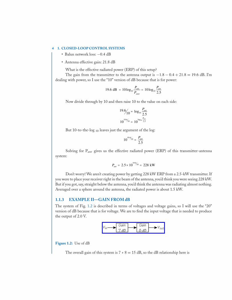
1.1.3 EXAMPLE II—GAIN FROM dBThe system of Fig. 1.2 is described in terms of voltages and voltage gains, so I will use the “20”version of dB because that is for voltage. We are to find the input voltage that is needed to producethe output of 2.0 V.
Figure 1.2: Use of dB
The overall gain of this system is 7 + 8 = 15 dB, so the dB relationship here is

1.2. BODE PLOTS 5
15 202 0
10dB = log.
Vin
Dividing by 20 and raising 10 to each side of the equation yields a result than can be solvedfor the voltage input:
10 10
2 0
10356
1520
2 0
15 20
10
=
= =
log .
.
V
in
in
V mV
1.2 BODE PLOTS
Hendrik W. Bode (1905–1982) was a pioneer in both controls and telecommunications. Unfortu-nately, he has the kind of name that has several ways of being pronounced: Bôw’dee or Bôw’dahor Bôw’duh. Mr. Bode probably used the Dutch pronunciation, which rhymes with Yoda, althoughYoda probably bears no resemblance to Mr. Bode.
Bode spent a good part of his career with the Bell Telephone Laboratories. He probably dida lot of work with signals and filters and communications lines. Doing this required him to plotthe gain of a system, both magnitude and phase, against frequency. Plots of this nature are a verycommon way of visualizing how a filter handles the various frequencies of a signal.
So of course Bode used the most powerful computer he had available. He would write outthe transfer function as a function of frequency and then have the computer plot two graphs, themagnitude of the transfer function and the phase angle of the transfer function, both against afrequency axis. He chose, like most practitioners of the day, to use a logarithmic frequency axis.
But there probably came a time when he got tired of doing all this computation. Even thoughhe probably had one of the more advanced computers of the day, the work was still time-consuming.Remember that this was in the late 1930s.
And what was Bode’s computer? Very likely a Keuffel&Esser Model 4080-3 Log-Log DuplexTrig sliderule, introduced by K&E in 1937. (You might have fun Googling it.) It was the top-of-the-line sliderule, although it was supplanted about ten years later with the Log-Log Duplex Decitrigrule that did angles in decimal degrees rather than degrees-minutes-seconds.
Bode developed the method of making the plot that carries his name to reduce the computationload on his sliderule. Today we use it mostly to display the magnitude and phase characteristics ofa transfer function, get quick estimates of how a system might behave, and help determine how toadjust system response.
Bode’s method is based on the ease by which the asymptotes of a magnitude or phase plot canbe drawn if the vertical axis is in dB or degrees and the horizontal axis is the logarithm of frequency.

6 1. CLOSED-LOOP CONTROL SYSTEMS
1.2.1 ASYMPTOTES MATHBode plots are for both magnitude and phase of transfer functions. We are going to restrict our lookto just magnitudes. In other words, we are going to plot |H(jω)| against log10 ω. We could be usinghertzian frequency just as well, but we’ll start with radians/second. For the magnitudes we will usedB.
While there are lots of possible configurations of |H|, we begin with just three:
H s s
H ss
a
H ss
a
( )
( )
( )
=
= +
=+
1
1
1
Since s = σ + jω and we are interested in just the sinusoidal steady-state response, we willrestrict the frequency to s = jω (or s = j2πf for hertz):
H j
H jj
a
H jj
a
ω ω
ω ω
ωω
( ) =
( ) = +
( ) =+
1
1
1
Our asymptotic analysis will start by finding the magnitude of H in dB (voltage dB) and thenseeing what the asymptotes look like on a graph of dB versus log ω.
From here on, I am going to omit the subscript “10” on the log symbol.Convert the first of the H forms to dB:
20 20log logH jω ω( ) =
Now we reason our way through the curve of |H| versus frequency:
• At ω = 1, |H| = 0 dB
• At ω = 10, |H| = 20 dB
• At ω = 100, |H| = 40 dB
And so on. 20 log ω defines a straight line whose slope is 20 dB for each step of 10 along thelog-ω axis. This step of 10 is a decade. Figure 1.3 shows this asymptote.
In other words, if one of the factors of H(s) is just s, this factor is plotted as a straight linepassing through (ω = 1, dB= 0) and sloping upward at 20 dB per decade. If one of the factors ofH(s) is 1/s, the line passes through (ω = 1, dB= 0) but slopes downward at 20 dB per decade.

1.2. BODE PLOTS 7
Figure 1.3: Bode plot for |H(s)| = s
Well, that wasn’t too bad. How about the second factor where H(s) contains the factor 1 +s/a? Take a look at the following manipulation of this factor, first getting its magnitude, then itsmagnitude in dB as a function of ω.
H jj
a
H ja
H ja
ω ω
ω ω
ω ω
( ) = +
( ) = +
( ) = + =
1
1
20 20 12
2
2
2
2log log
00
21
10 1
2
2
2
2
log
log
+⎛⎝⎜
⎞⎠⎟
= +⎛⎝⎜
⎞⎠⎟
ω
ω
a
adB
That looks messy, but let’s not get eaten by the alligators while we are working in the swamp.Remember that our goal is to get the asymptotes of the function, not the exact path. So we’ll lookat what happens in two regions, one when ω is much smaller than a and getting smaller, the otherwhen ω is much larger than a and getting larger.
As ω gets much smaller than a, our term becomes
lim ( ) lim logω ω
ω ω→ →⎡⎣ ⎤⎦ = +
⎛
⎝⎜
⎞
⎠⎟
⎡
⎣⎢
⎤
⎦⎥
=
0 0
2
210 1
1
H ja
00 1 0log( ) =
This says that the asymptote for small values of ω is a horizontal line at 0 dB.What does the asymptote in the other direction look like? Here’s the math:
8 1. CLOSED-LOOP CONTROL SYSTEMS
lim ( ) lim logω ω
ω ω→∞ →∞
⎡⎣ ⎤⎦ = +⎛
⎝⎜
⎞
⎠⎟
⎡
⎣⎢
⎤
⎦⎥
=
H ja
10 1
1
2
2
00 202
2log( ) log( )
ω ωa a
=
Let’s do the same thing we did with 20 log ω:
• At ω = a, |H| = 0 dB
• At ω = 10a, |H| = 20 dB
• At ω = 100a, |H| = 40 dB
This defines a straight line whose upward slope is 20 dB per decade. Hmmm, haven’t we justheard about one of those?
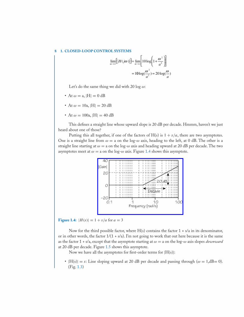
Putting this all together, if one of the factors of H(s) is 1 + s/a, there are two asymptotes.One is a straight line from ω = a on the log-ω axis, heading to the left, at 0 dB. The other is astraight line starting at ω = a on the log-ω axis and heading upward at 20 dB per decade. The twoasymptotes meet at ω = a on the log-ω axis. Figure 1.4 shows this asymptote.
Figure 1.4: |H(s)| = 1 + s/a for a = 3
Now for the third possible factor, where H(s) contains the factor 1 + s/a in its denominator,or in other words, the factor 1/(1 + s/a). I’m not going to work that out here because it is the sameas the factor 1 + s/a, except that the asymptote starting at ω = a on the log-ω axis slopes downwardat 20 dB per decade. Figure 1.5 shows this asymptote.
Now we have all the asymptotes for first-order terms for |H(s)|:• |H(s)| = s: Line sloping upward at 20 dB per decade and passing through (ω = 1,dB= 0).
(Fig. 1.3)

1.2. BODE PLOTS 9
Figure 1.5: |H(s)| = 1/(1 + s/a) for a = 3
• |H(s)| = 1 + s/a: Two lines, one starting at ω = a and going to the left at 0 dB; the otherstarting at ω = a and sloping upward to the right at 20 dB per decade. (Fig. 1.4)
• |H(s)| = 1/(1 + s/a): Two lines, one starting at ω = a and going to the left at 0 dB; the otherstarting at ω = a and sloping downward to the right at 20 dB per decade. (Fig. 1.5)
One final remark on these slopes: Only 20 dB per decade and integral multiples are possible.That means ±20 or ±40 or ±60 or ±80 and so on, but not 15 or 23.98 or anything else.
It is sometimes convenient to state these slopes in dB per octave. 20 dB per decade is the sameas 6 dB per octave, where an octave is a factor of 2.
1.2.2 PUTTING THE ASYMPTOTES TOGETHERGosh! I now know all about asymptotes and I can draw all sorts of lines that show me somethingabout factors of |H(s)|. That sounds like something I’ve always wanted to…. Um, I’m not sure that’strue. So, OK, why do I need those asymptotes?
Well, consider. Suppose I have a system, described by H(s) in one of its various forms likeH(s) or H(jω) or H(j2π f ). It’ll look something line this:
H sA constant Some factor in s
Another s te( ) = ( )( )
rrm A third one( )( )
This H(s) is a combination of factors. The first is divided by the other two. Those bottomtwo are multiplied together. Now remember what logs do for us. Multiplication becomes addition;division becomes subtraction. So this H(s), when converted to |H(jω)| and then converted to dB(logs, that is) becomes
log ( ) log( ) log
lo
H j A constant Some factor in sω = +− gg logAnother s term A third one−

10 1. CLOSED-LOOP CONTROL SYSTEMS
That says that we create the asymptotes for the individual factors, one by one, and then weadd or subtract as appropriate to get the final Bode plot. So if you were worried how this gets backto Bode and the plots, that is how it’ll appear. (OK, so you weren’t worried….)
Actually, it’s even easier. If we have the asymptotes for the various factors, we just add them onthe graph—no subtraction. Why no subtraction? Because we have already developed the asymptotesfor a factor in the denominator that includes the sign—that’s where we got the downward-at-20-db/decade slope.
The basic algorithm for generating Bode plots:
• Rearrange H(s) to put all the factors in the form of either s or 1 + s/a
• Draw the asymptote for the constant term, if any, converted to dB (a horizontal straight line)
• Draw the asymptote for the s term, if any, passing through ω = 1 at 0 dB. The line slopesupward at 20 dB per decade if the s is in the numerator, downward if it’s in the denominator
• Draw the asymptotes for any factors in the numerator by drawing a horizontal line from ω =a to the left at 0 dB and a second line with an upward slope of 20 dB per decade from ω = a.
• Do the same thing for any factors in the denominator, but sloping downward at 20 dB perdecade
• Add these asymptotes graphically
Now some examples.
1.2.3 EXAMPLE III—BODE PLOT FOR ONE POLEPlot the Bode magnitude plot for
H ss
( ) =+4000
2000
First, convert this to the 1 + s/a form by dividing through by 2,000:
H ss
( ) =+
2
12000
Now convert the numerator factor (2) to dB:
20 2 6log = dB
Draw this on the plot (Fig. 1.6, dotted line at 6 dB).Now plot the asymptotes of the denominator, which are a line to the left from ω = 2,000 at
0 dB and a line sloping down to the right, starting at ω = 2,000, with a slope of −20 dB per decade(Fig. 1.6, dotted line).

1.2. BODE PLOTS 11
Figure 1.6: Example III
Sum the asymptotes.To the left of ω = 2,000, 0 + 6 = 6 dB.To the right,move the downwardslope up by 6 dB. The result is the solid lines of Fig. 1.6.
1.2.4 EXAMPLE IV—BODE PLOT FOR POLE AND ZEROPlot the asymptotes for the magnitude of this H(s):
H ss
s( ) =
+5
500
Convert:
H ss
s( ) =
+
5500
1500
The d-c constant is 5/500 = 0.01, which in dB is −40 dB. So this asymptote is a horizontalline at −40 dB (Fig. 1.7).
The s in the numerator is a line sloping upward to the right and passing through ω = 1 and0 dB (Fig. 1.7).
The asymptotes for the denominator factor are two lines. One starts at ω = 500 and goeshorizontally to the left at 0 dB. The other starts at 500 and goes downward to the right at −20 dBper decade (Fig. 1.7).

12 1. CLOSED-LOOP CONTROL SYSTEMS
Figure 1.7: Example IV
Now add them, working from left to right to get the result shown in Fig. 1.7. Notice thatadding a slope of +20 dB per decade to a slope of −20 dB per decade yields a flat line (a slope of 0dB per decade).
1.2.5 EXAMPLE V—BODE PLOT FOR TWO POLESGiven
H ss
s s( )
.= ×+( ) +( )
7 5 10
150 2500
4
Convert to
H ss
s s( )
.=+
⎛⎝⎜
⎞⎠⎟ +⎛⎝⎜
⎞⎠⎟
0 2
1150
12500
The numerator constant is 0.2,which is −14 dB,which is a horizontal line at −14 dB. (Fig.1.8)
The numerator factor s is an upward slope of 20 dB per decade passing through ω = 1 and0 dB.
The denominator has two factors. One breaks at ω = 150 and the other at ω = 2, 500. Theirflat parts are along 0 dB. One breaks downward at −20 dB per decade at ω = 150 and the otherbreaks downward at ω = 2, 500.
The sum of these finishes the plot in Fig. 1.8.

1.2. BODE PLOTS 13
Figure 1.8: Example V
1.2.6 EXAMPLE VI—BODE PLOT TO TRYThis H(s) has an s in the denominator:
H s
s
ss
( ) =+
⎛⎝⎜
⎞⎠⎟
+⎛⎝⎜
⎞⎠⎟
18 1200
13000
It’s already converted to proper form.The constant term is 18, which is 20 log 18 = 25 dB.The numerator’s factor is level at 0 dB to the left of ω = 200 and slopes upward at 20 dB per
decade to the right of ω = 200.The s term in the denominator is a downward slope of −20 dB per decade passing through
ω = 1 and 0 dB.The denominator term breaks downward to the right at ω = 3,000.Their sum is…left as an exercise for you. It passes through (ω = 0, 25 dB) sloping downward
to ω = 200, flattens out at −21 dB, then continues the downward slope starting at ω = 3,000.
1.2.7 WHAT DO THESE MEAN?The four examples we’ve just done describe three different types of filters. While we haven’t provenit, the break frequency of a circuit is the “joint” between the asymptotes. So in Example III (Fig. 1.6),

14 1. CLOSED-LOOP CONTROL SYSTEMS
we have a low-pass filter with a break frequency of ω = 2,000 radians/second. Below that frequency,the filter passes signals with a gain of 6 dB. Above 2,000, it begins to cut off the signal.
Example IV (Fig.1.7) is a high-pass filter with a break frequency of 500 radians/second.Abovethat, it passes the signal with what the plot shows to be a 14-dB gain. Below that, it diminishes thesignal.
Example V is a band-pass filter (Fig. 1.8). It has a pass-band gain of 27 dB and breaks at 150and 2,500 radians per second.
1.2.8 FINISHING UP BODE’S WORKHendrik Bode didn’t do this just for the asymptotes, and he didn’t do it just for first-order factors.I’m leaving the higher-order factors to another course, but we do need to see how Bode constructedthe actual response curve from the asymptotes.
Part of the answer of how he did it is obvious: the curve must conform to the asymptotes. Buthe devised a scheme that enabled him to sketch in the actual curve within a precision of about halfa dB of the exact curve that he could have calculated using his Log-Log Duplex Trig sliderule.
Here are the steps, which I’ll draw on the Bode plot of Example V. (See Fig. 1.9.)
Figure 1.9: Example V complete
• Inside the corners at ω = 150 and ω = 2, 500, place a point 3 dB inside the corner.That meansdropping down 3 dB from the corner to mark the point.
• Now let’s work near the corner at ω = 150. From this corner, move to the left by a factor oftwo, which puts us at ω = 75. Place a point 1 dB inside the curve.

1.3. CLOSED-LOOP SYSTEMS 15
• Likewise, move from this corner to the right by a factor of two (i.e., ω = 300 and place a point1 dB inside the curve.
• Do the same for the other corner at ω = 2, 500, moving down to 1,250 and up to 5,000.
• Now eyeball a smooth curve following the asymptotes but passing through the six points thatyou marked.
If you have drawn carefully and then compare with results from Maple or Matlab, you shouldhave trouble telling them apart. (Figure 1.9)
That’s Bode’s genius.
1.3 CLOSED-LOOP SYSTEMSOne way to start looking at closed-loop control systems is to look at open-loop systems first. Doingthis might give us some perspective on the why of closed-loop.
The system of Fig. 1.10 is an open-loop control system. The input to the system is r(t). That
Figure 1.10: Open-loop, t domain
input is to produce a desired outcome, y(t). An example might be a system (the G block) consistingof a power amplifier and a d-c motor. A voltage r(t) drives the input of the amplifier. The amplifieramplifies this voltage to make the d-c motor run. The output y(t) is the desired rpm of the motor.
This turns out to be a not-so-hot control system! It does control the speed of the motor but notvery well. For example, suppose there is a linear relation between the input voltage and the rpm of themotor. To keep things simple, one volt at the input r(t) makes the motor output y(t) = 1,000 rpm.
Now add a load to the motor. It naturally slows down, so y(t) is less than 1,000 rpm. But r(t)is still 1 volt, so we think the motor should still be producing 1,000 rpm. Our system is not robustin that it cannot respond to changes at the output.
So far, I’m thinking in the time domain with my variables as functions of t . We won’t continuein the time domain but instead will switch to the frequency or phasor domain and consider operationjust in the sinusoidal steady state. Figure 1.11 shows our simple open-loop system in phasor domain.
Now R(s) is the reference signal and Y(s) is the output. The amplifier and the motor in ourexample are G(s). But switching to the phasor domain doesn’t do a thing to improve our system. Itis still open-loop and the input reference is not aware of any changes in the output. It is still notrobust.
It’s time to close the loop.

16 1. CLOSED-LOOP CONTROL SYSTEMS
Figure 1.11: Open-loop, s domain
1.3.1 CLOSING THE LOOPClosed-loop systems close the loop by watching the output, then feeding back that informationto the input. What comes back is compared with the reference. If they don’t match, the systemis adjusted to make them match. Now our system can be robust, because a change in the outputchanges the input to compensate for the change in the output.
Figure 1.12 shows the basic closed-loop system. Here’s what the various pieces do:
Figure 1.12: Closed-loop system
G(s) is the forward path. It is made up of the plant (like the d-c motor of my open-loopexample) and the driver for that plant (like the amplifier in my example).
H(s) is the feedback device that gets information from the output and delivers it to be comparedwith the input (like a tachometer).
R(s) is the reference signal that establishes what we are trying to do (like the input voltage inmy example).
Y (s) is the output of the system (like the rpm of the d-c motor).
E(s) is the error signal, which is the difference between the reference R(s) and the actualoutput Y(s).

1.3. CLOSED-LOOP SYSTEMS 17
The summer is the comparator, subtracting the feedback information from the reference tocreate the error signal E(s).
The two blocks in the system, G(s) and H(s) are not functions of time—they stay constant asfar as we are concerned. Yet this is not 100% true.They perhaps drift slowly with time or temperatureor voltage change. For our analysis, though, we consider them to be static, meaning not time-varying.
If anything in this system needs to be stable and predictable, it is H(s). It is important thatH(s) observes the output and reports the results to the summer in a very consistent manner. We willtake some care to be sure H(s) in the feedback path can be expected to behave.
1.3.2 ANALYZING THE LOOPThe output Y(s) depends on the error signal E(s) driving G(s):
Y s G s E s( ) ( ) ( )=
The error signal E(s) is the difference between the reference R(s) and the signal fed back fromthe output:
E s R s H s Y s( ) ( ) ( ) ( )= −
Combining these two equations yields the classic description of a feedback system:
Y sG s
G s H sR s( )
( )
( ) ( )( )=
+1
Everyone who works with closed-loop systems knows this one by heart! One way of statingit mentally is, “Forward gain over 1 plus loop gain.” The forward gain is the path from left to right,namely, G(s). The loop gain is clockwise around the loop, namely, G(s)H(s). Another common wayto say this is, “G over 1 plus GH.”
Now let’s examine the characteristics of the two big players in this equation, G(s) and H(s).We can make the following generalizations, that are usually true in a control system:
• G(s) is usually a heck of a lot bigger than 1. How “heck of a lot”? Back to my motor example.A small error voltage must drive a large motor, so the gain needed to do this is large. We canwrite something like G >>> 1.
• H(s) is generally not larger than 1. While it can be 1, meaning that the output is fed backwithout change, bigger than 1 is bad. Why? Because this implies an amplifier, which hasinaccuracies like long-term drift and change due to voltage supply changes and so on. We wantH(s) to be as perfect as possible because it is measuring how well our reference is controllingthe output. So H < 1.
Now I’m a bit stuck for notation. I’ve used R and E and G and Y and H, which is prettycommon but by no means universal. However, H is now “used up” and I can’t use it for labeling the

18 1. CLOSED-LOOP CONTROL SYSTEMS
overall transfer function as in previous chapters. I’m going to use TF for “transfer function” to meanthe overall relationship between output and input:
TF sG s
G s H s( )
( )
( ) ( )=
+1
If G >>> 1 and H < 1, look what happens to TF:
TFG
GHG H GH
TFG
GH H
=+
>>> < >>
≅ =
11 1 1
1
for and ,
In other words, the ideal, perfect system has a transfer function that is simply 1/H. But if thesystem is perfect, it can’t work! We can see this by figuring out what the error signal E(s) will beunder these perfect conditions:
E R HR
HY
HR= − = =0
1for
The error signal E(s) drives the amplifier or whatever is in the forward path. If E(s) is zero,it can’t drive anything. If nothing is driven, there is no output. So the system can’t work. How closecan we get to “perfect?” We need to look at error in the desired output Y(s).
1.3.3 EXAMPLE VII—TRANSFER FUNCTIONA certain plant requires a gain of 40 dB ± 5%, which is a gain of between 38 and 42 dB. This meansthat the reference signal R(s) is to be amplified by 40 dB to produce the output Y(s).The amplifier inthe forward path is typical of amplifiers: its gain is not “perfect” but varies from 104 to 105. (Forwardgain is often called the open-loop gain.)
First we consider the ideal situation where TF(s) = 1/H(s):
TF
H sTF s
= = =
= =
40 10 100
10 01
40 20dB
( )( )
.
Now find the system gain TF(s) at the ends of the range of amplifier gain:
1.3. CLOSED-LOOP SYSTEMS 19
for
for
G s
TF s
G s
( )
( ).
( )
=
=+ ( )( )
=
=
10
10
1 10 0 0199
1
4
4
4
00
10
1 10 0 0199 9
5
5
5TF s( )
..=
+ ( )( )=
The system gain is supposed to be 100. Depending on the actual gain of the amplifier, thesystem gain is really between 99 and 99.9. That’s an error of between 1% and 0.1%. In dB, this rangeis 39.91 to 39.99 dB, well within the 40±5% specification. The system won’t be perfect until G isinfinite!
1.3.4 FRACTIONAL ERRORThe ideal or perfect system has a transfer function of 1/H(s). But we can’t have that and insteadhave some less-than-perfect transfer function TF(s). We define the fractional error as
E H sTF s
TF s
H s
G s
G s H sG s
frac =−
=−
+
1
11
( )( )
( )
( )( )
( ) ( )( )
11
1
+
=
G s H sG s H s
( ) ( )( ) ( )
Fractional error is just 1 over the loop gain.
1.3.5 EXAMPLE VII CONTINUEDFor G = 104, the gain was 99.0, an error of 1%. The fractional error is
E frac = ( )( )=1
10 0 010 01
4 ..
which is 1%. For G = 105, the gain was 99.9, an error of 0.1%. The fractional error is
E frac = ( )( )=1
10 0 010 001
5 ..
which is 0.1%.Suppose G falls to 103. The fractional error is

20 1. CLOSED-LOOP CONTROL SYSTEMS
E frac = ( )( )=1
10 0 010 1
3 ..
which is 10%.
1.3.6 EXAMPLE VIII—MOTOR SPEED CONTROLThe d-c motor of Fig. 1.13 is to produce 2,000 rpm with a control voltage of 2 volts. The motor’s
Figure 1.13: D-c motor
response is linear, so a control voltage of 0 to 2 volts is to produce 0 to 2,000 rpm.The motor constantis km = 50 rpm/V.
If we do this job using an open-loop system, we need an amplifier with a gain of A (seeFig. 1.14):
Figure 1.14: D-c motor: open-loop control
V n
n A V
A
C m
m C
= ⇒ == ( )( )=
2 2000
50
20
V rpm
The open-loop system needs a gain of 20 to drive the motor so 2 volts input produces 2,000rpm. But what happens to the motor speed when the load on the motor increases? Very simply, thespeed just goes down. The control voltage is still 2 V, but the speed is no longer 2,000 rpm.
Well, how about the closed-loop control system in Fig. 1.15? (Note the use of units in theblocks—it’s not a bad idea to do this.)
The tachometer must “match” the output to the input. VC at 2 volts corresponds to nm =2, 000 rpm. This means the tachometer constant must be kt = 2/2000 = 0.001 V/rpm. This meetsour requirement that H(s) be no larger than 1.

1.3. CLOSED-LOOP SYSTEMS 21
Figure 1.15: D-c motor: closed-loop control
That takes care of H(s). Now how about G(s)? It’s tempting to say that we already have,because in the open-loop system in Fig 1.3-5, the amplifier and the motor together have a gainG(s) = (20)(50) = 1,000 rpm/V. That seems perfect because 2 V in gives 2,000 rpm out.
But the amplifier is no longer amplifying the input voltage Vc; it’s amplifying the error voltagefrom the summer. If we want “perfect” output, meaning exactly 2,000 rpm for 2 V in, we need theamplifier to have infinite gain. How do I get this conclusion? Look at the fractional error:
EGH G s
frac = =1 1
0 001. ( )
For the fractional error to be 0 (i.e., perfection), G(s) must be infinite. So the next questionis, how much error are you willing to accept in your system?
Let’s say we’ll accept 2% fractional error:
EG s H s
G s
A
frac = =
=( )( )
= ×
=
0 021
1
0 02 0 0015 104
.( ) ( )
( ). .
kk A
Am =
=50
1000 V/V
The actual maximum rpm for Vc = 2 V will be
nm = ( )( )+ ( )( )( )
=21000 50
1 1000 50 0 0011961
.rpm
Instead of 2,000 rpm, we get 1,961 rpm. Hmmm, maybe we want better than that. How about1% fractional error?

22 1. CLOSED-LOOP CONTROL SYSTEMS
EG s H s
G s
Ak
frac
m
= =
=( )( )
=
=
0 011
1
0 01 0 001105
.( ) ( )
( ). .
===
50
2000
A
A V/V
The outcome depends on what error you’ll accept and how much gain you are willing to payfor in the amplifier. Notice that as the gain goes up, the fractional error improves.
1.3.7 EXAMPLE IX—LINEAR POSITIONERThe linear positioner shown in Fig. 1.16 can position an object over a range of 400 mm under control
Figure 1.16: Positioner to be controlled
of a voltage ranging from 0 to 4 V. The positioner’s constant is
kp = 0 5. mm/mV
The position x is to be precise to within ±0.5 mm.Two laser range finders are available with sufficient precision. Each produces a voltage pro-
portional to distance:
#1: mV/mm
#2: mV/mm
V
Vf
f
==
2
20
Range finder #1 is less expensive, so let’s try to design with it first. The maximum outputvoltage of range finder #1 will be
Vf =⎛⎝⎜
⎞⎠⎟( ) =2 400 800
mV
mmmm mV
Hmmm, that should be OK. We can just put a gain of 5 in the feedback path to get the propercomparison with the 4-V control voltage.
No way! We must not do this! Putting gain in the feedback path means sacrificing the precisionof that path. Remember that the feedback should be as precise as possible and should be no greaterthan 1.

1.3. CLOSED-LOOP SYSTEMS 23
Let’s try again with range finder #2:
Vf =⎛⎝⎜
⎞⎠⎟( ) =20 400 8
mV
mmmm V
That’s twice as big as we need. But it’s OK to reduce that output because it can be done withpassive components. A simple voltage divider made of precision resistors will probably do the job.
The complete system is shown in Fig. 1.17. Our final job is to select the gain A of the amplifier.
Figure 1.17: Positioner controller
We do this by making the fractional error fit the original specifications, which said we wanted aprecision of no worse than ±0.5 mm.
EG s H s
A
A
frac = =
=( )( )( )( )
0 5
400
1
1
0 5 20 12
.
( ) ( )
.
mm
mm
==160
I’ll check this result at Vc and see if it produces a value of x within ±0.5 mm of 400 mm:
G s
H s
T
( ) .
( )
= ( )( ) == ( )( ) =
160 0 5 80
20 12 10
mm/mV
mV/mm
FF s( ) .=+ ( )( )
=80
1 80 100 099875 mm/mV
At the full control voltage Vc = 4.000 V:
x = ( )( ) =0 099875 4000 399 5. . mm

24 1. CLOSED-LOOP CONTROL SYSTEMS
Great! The error is exactly 0.5 mm. Also note that
G sH s
( )( )
.= =801
0 1
I’ll be adding to this example in the next section.
1.4 BANDWIDTHThe example of the positioner that I’ve just done isn’t very realistic. Aw, gee, and you thought all theexamples in textbooks were real? Sorry to disappoint you…. What’s wrong with this one?
Think about how a positioner might work.Can it move instantly from one position to another?Does it perhaps dilly-dally? How does it really respond in the world of mass and dampers and finiteforces and the like? Right! It can’t act instantly. So our model of the positioner as just a box with aconstant kp doesn’t describe the device very well.
Suppose this positioner is a first-order system. (It’s really probably second-order, but let’s keepthis fairly simple.) As a linear first-order system, its response to a step is an exponential. Figure 1.18shows a possible response. The time-domain equation for this response to a step vin(t) is
Figure 1.18: Physical system response
x t k v t ep int( ) ( )= −( )−1 τ
Take the Laplace transform of this to get
X sk V
s
k V
sk
V
s sX s
V s
k
s
p in p inp
in
in
p
( )
( )
= −+
=+
=
ττ τ
τ
1
1
1
++1

1.4. BANDWIDTH 25
Figure 1.19: Realistic system
The positioner block in our system diagram now includes this first-order characteristic. Fig-ure 1.19 is more realistic. Note that it still will have a d-c response (i.e., s = 0) of 0.5 mm/mV. Thathasn’t changed. Just the time it takes to actually move to a position has been added.
1.4.1 EXAMPLE IX CONTINUEDTo get the time response of a device, we must characterize it from physical measurements, somethingwe’ll do in Chapter 2. Figure 1.20 is an example of a graph, taken from an oscilloscope, that showshow my positioner responds to a step input.
Figure 1.20: Characterizing
Remember that the time constant is the point on the exponential where the curve has 1/e togo to reach its final value. In this graph, the total excursion is 120 mm, so 1/e yields
1120 44 1
140 44 1 95 9e
x
t
=
= − ==
.
. .
mm to go
so mm
when ττ = 32 ms
The new block diagram for the positioner is Fig. 1.21. We need the new transfer functionTF(s) for this system. But before doing this for the positioner, we need a brief excursion into a wayto simplify our algebra.

26 1. CLOSED-LOOP CONTROL SYSTEMS
Figure 1.21: Positioner controller #2
1.4.2 SIMPLIFYING TF(s)We already know that the transfer function of a closed-loop system is
TF sG s
G s H( )
( )
( )=
+1
First, note that H is generally not a function of s—it’s just a number. Now, if we split G(s)into a numerator and a denominator, things get less messy:
G sN s
D s( )
( )
( )=
The result is a simpler way to do the algebra to get TF(s):
TF s
N s
D sN s
D sH
N s
D s H N s
( )
( )( )( )( )
( )
( ) ( )
=+
=+
1
Now back to the example.
1.4.3 EXAMPLE IX CONTINUED SOME MOREFor our improved system,
G ss
H( ).
,=+
=80
0 032 110
mm/mVmV/mm
Using the simpler way of getting TF(s) yields

1.4. BANDWIDTH 27
N s D s s
TF ss
( ) , ( ) .
( ).
= = +
=+ + ( )( )
80 0 032 1
80
0 032 1 10 80
==+
80
0 032 801. s
We need to present functions like these in standard form, which means that the polynomialsin s have “1” as the coefficient of the highest-order s term. Doing that here gives us the standardform for TF(s):
TF ss
( ).
.=
+ × −
0 099875
1 39 95 10 6
mm
mV
Check this result for d-c to see if it gives the same result as before. At d-c, s = 0, so thetransfer function is
at d-c,mm
mVTF( ) .0 0 099875=
OK! It came out the same. That helps to check our work.
1.4.4 FASTER RESPONSESomething else has happened, though, that is very important to notice. The original positioner,without the closed-loop control system, has a time constant of 32 ms. That’s what we measuredwhen we characterized the positioner.
Take a look at the result of TF(s) after we have built the positioner into the closed-loop controlsystem. The time constant of the actual response is
τ = × ≅−39 95 10 406. μs
Feedback speeds up the response!
1.4.5 BODE REPRESENTATIONIt turns out to be useful to plot on a Bode diagram the functions G(s), 1/H, and TF(s). I’ll plot themas functions of s = jω in Fig. 1.22.
First let’s do G(s),
G ss
( ).
=+
80
1 0 032
• At d-c, G(0) = 80, which is 20 log10 80 = 38 dB, so the plot starts flat at 38 dB.
• The break frequency is at ωb = 1/0.032 = 31.25 radians/second, so the plot of G(s) breaksdownward at 20 dB/decade at ωb

28 1. CLOSED-LOOP CONTROL SYSTEMS
Figure 1.22: Bode diagram for positioner controller #2
Now let’s do 1/H. Wait! you say. Why 1/H and not just H? Hold on for a bit and you’llsee, but here’s a clue: recall that the “perfect” system response is 1/H if G is very very large. SinceH = 10 mV/mm, 1/H = 0.1, which is −20 dB. (Note the minus sign.) This is a straight line onthe Bode diagram.
From the Bode diagram we now have, we can deduce a few things:
• For ω < 10,000 radians/second, |G| � 1/H. We can see that on the plot, because the Gasymptote is 58 dB above 1/H. Under this condition, the actual transfer function TF(s) is veryclosely represented by just 1/H.
• For ω > 100,000 radians/second, |G| � 1/H. Again, we can see the dB difference on the plot.Under this condition, the actual transfer function TF(s) is closely represented by G(s) alone.
• The dotted line on the Bode plot of Fig. 1.21 is the result of combining the trace of 1/H belowwhere they cross and the trace of G(s) above where they cross.
• The break frequency of the complete closed-loop control system is where the two asymptotescross at 25,000 radians/second (where the actual curve is 3 dB inside the corner).
Bandwidth is the frequency from 0 to the break frequency. Look what has happened to thebandwidth of the system:
• The original G(s) breaks at 31.25 radians/second, so its open-loop bandwidth is 31.25 radiansper second.

1.5. STABILITY 29
• The closed-loop system breaks at 25,000 radians/second, so its bandwidth is increased to25,000 radians per second.
Feedback increases system bandwidth!
The new bandwidth is defined by where G crosses 1/H: ωnew = ωold(1 + GdcH).
1.5 STABILITYWe are not going to worry much about system stability in this course except to consider that systemscan be designed and built that are not stable. What does stable mean? Firm, steadfast. Hmm, weneed more than that.
A system is stable if its poles are in the left half plane. Ugh. OK, what’s that saying? The polesare the roots of the denominator of the transfer function TF(s). Those roots must be to the left ofthe imaginary axis on the complex plane.
The denominator of the example we’ve just been working through is
1 0 032+ . s
Setting that to zero gives is the position of this pole:
1 0 032 0
31 25
+ =
= −
.
.
s
s s-1
The result is a negative value, so this root is in the left half of the complex plane and lies onthe real axis at −31.25 seconds −1
If the roots happened to be complex values such as for a quadratic, the real part of each of theroots must be negative.
There is much more to stability, including questions of stable but dangerous. For example, ifyou car has bad front shocks and you hit a chuck hole with one front tire, the front end steeringand suspension may go into violent oscillation. The mechanical system is technically stable if theoscillation damps out, but the vehicle is unsafe nevertheless.
1.6 MORE EXAMPLEWe really haven’t finished Example IX yet, but I’ll cheat and finish it as Example X. Also, we haven’tlooked at how one might select a reasonable gain when designing a control system. Although wenow know that “perfect” response comes with a gain G of infinity, we know we can’t do that!
1.6.1 EXAMPLE X—REALLY IX CONTINUED AGAINWe started Example IX with a positioner that moved instantly from one position to another. Thenwe gave the positioner a first-order exponential response. We saw that the feedback control made

30 1. CLOSED-LOOP CONTROL SYSTEMS
the system respond much faster and its bandwidth was much higher. “Faster” and “higher” go hand-in-hand.
We neglected the amplifier, though, by assuming that it just amplifies. Which of course itdoes. But not instantly. It like the positioner cannot go instantly from one output to another. So let’sassume that, in its simplest form, it too follows an exponential trajectory.
I’m going to change the amplifier to one with a cutoff frequency of 100 radians/second, whichcould represent a heavily designed, elderly power amplifier. (That’s 16 Hz, which is very low!)
If the cutoff frequency is 100 radians/second, the time constant of this first-order system is
τ = =1 100 10 ms
Compare 10 ms with the 32-ms time constant of the positioner and note that the amplifier is“faster” in responding than then positioner. This might imply that the amplifier won’t be much of afactor in how our system responds.
Figure 1.23 is the new amplifier in the system.Calculations to get the transfer function produce
Figure 1.23: Positioner controller #3
a quadratic in the denominator this time:
G ss s
s s
( ).
.
.
. .
=+ +
=+ +
160
0 01 1
0 5
0 032 180
0 00032 0 042 12
TTF sN
D H N
s
G
G G
( )
.
. .
=+
=× + ×
0 099875
0 3995 10 52 43 106 2 +6 1s
Let’s see how this second-order system behaves. We’ll do this in more detail in Chapter 2.Doing this will show that the damping reatio is 0.0415, way less than 0.5. That means the systemis not only underdamped, it is close to oscillatory.

1.6. MORE EXAMPLE 31
That will yield very poor operation because the positioner’s arm will overshoot its goal andthen oscillate numerous times before settling down to where it belongs. There’s just not enoughdamping.
The Bode diagram for this system (Fig. 1.24) is instructive. The d-c value is still 80. The plot
Figure 1.24: Too much underdamping
of 1/H has not changed. There are now two break frequencies:
ω
ω
1
2
1
0 03231 25
1
100100
= =
= =
.. rad/s
rad/s
(In order to get the peak of the curve as shown, I had to calculate the actual value of |TF| atseveral points near the crossing.)
I guess we had better try a faster amplifier (Fig. 1.25):
Figure 1.25: Another amplifier

32 1. CLOSED-LOOP CONTROL SYSTEMS
τω
==
100
10 000
μs
rad/sb ,
The new Bode diagram is Fig. 1.26. Following the same analysis as before, we get a value for
Figure 1.26: Still too much underdamping
the damping ratio (0.32) that is still too small for “decent” behavior.OK, I’ll try once more with an amplifier with a cutoff frequency of 25,000 radians/second
(about 4 kHz). The time constant is 40 μs. Figure 1.27 is the block for this newest amplifier. TheBode diagram of Fig. 1.28) shows that the peak where |G| crosses 1/H is much smaller and thedamping ratio is 0.5.
Actually, this system is right on the edge of being acceptable. “Acceptability” for second-order(and higher) systems is defined here as having a damping factor between 0.5 and 1. We can use theBode diagram to get meet this requirement:
Here is a general rule for “acceptable,” said two different ways:
• The 1/H line crosses the line for |G| before the second break frequency.
• 1/H crosses |G| before the second dive.
In this example, the crossing is right at the break that starts the last dive.
1.6.2 EXAMPLE XI—FINDING MAXIMUM GAINThis is an example of how we can choose the forward gain from a Bode construction. Suppose mysystem is third-order:

1.6. MORE EXAMPLE 33
Figure 1.27: Proper amplifier
Figure 1.28: Borderline underdamping
G sk
s s s
H
( ). . .
.
=+( ) +( ) +( )
=
200
1 0 01 1 0 05 1 0 2
0 5
Our goal is to find the maximum acceptable k for proper operation. This means finding k sothe damping factor is no smaller than 0.5.
Assume the numerator 200k = 1 = 0 dB—we’ll find k later. Start plotting the asymptotes ofG(s). The break frequencies are
ω
ω
ω
1
2
3
1
0 25
1
0 0520
1
0 01100
= =
= =
= =
.
.
.
rad/s
rad/s
radd/s

34 1. CLOSED-LOOP CONTROL SYSTEMS
See Fig. 1.29. Each break increases the downward slope by another 20-dB per decade.
Figure 1.29: Determining k
Plot 1/H is in its proper place in the Bode diagram:
1 1
0 52 20 2 610
H= = → =
.log dB
We know that 1/H must cross |G| before the second dive. This second break is at 100 radi-ans/second. The question is how far can I shift upward the line for |G| to make 1/H cross at thissecond break?
I’ve marked the distance to raise |G| on the Bode plot in Fig. 1.29. The curve can be movedup as much as 18 dB.
Where I assumed the numerator is 1, we now see it can be 18 dB. So
max
.
G
k
k
=
==
18
200 10
0 0397
18 20
dB
so
That’s the largest k that doesn’t produce a damping factor less than 0.5. If we increase theoverall gain any more, we go below 0.5. We can choose a smaller gain, however, to get an even largerdamping factor and even less oscillation.
1.7 SUMMARYThis has been a packed chapter! It covers two major topics, Bode plots and feedback, with two minorones, dB and stability. But these all fit together to help us describe closed-loop control systems.

1.7. SUMMARY 35
We use dB to compare signal levels, amplifier gains, and the like because it’s a convenient yetlogarithmic value. It is basic to Bode plots.
Bode plots are a quick way to lay out the asymptotes of a gain magnitude in dB versus thelogarithm of frequency. While Bode was doing this as a way to get actual plots without a lot ofcalculation, we use this primarily for insight into system operation.
There are only three asymptotes in Bode plots as we have been using them: level, upward at20 dB per decade, or downward at the same slope. These slopes can be integer multiples of 20 aswell. Once we have the asymptotes, we can sketch the actual curve if we want to, but this isn’t usuallynecessary.
Closed-loop control systems, sometimes called feedback systems, achieve more robust opera-tion of a plant such as a motor or solenoid. By comparing the input signal with a report on the actualoutput, the system makes changes to make the output follow the input It does this even in the faceof most perturbations.
For proper operation, the device or circuit that feeds back to the input a report on the outputmust be stable and precise. For the perfect system, the transfer function from input to output is thereciprocal of the feedback device’s transfer function.
But unless the gain of the forward path is infinite, we can’t have perfection. We use fractionalerror to measure how closely we come to this ideal system. Choosing an acceptable fractional errorallows us to choose the necessary forward gain.
Controlling a plant with a closed-loop system improves two related characteristics of theplant’s operation: response time and bandwidth. Our designs must consider appropriate amounts ofunderdamping, too. This can be determined from the Bode plot of G(s) and 1/H by making surethat 1/H crosses G(s) before the second break frequency of G(s).
This discussion of closed-loop systems is very basic. It ignores most stability questions. Itignores systems with complex roots. So if you need to work extensively with such systems, do a lotmore study!
Where do the parameters of the system elements come from? Where did we get the timeconstant for the positioner, for example? By appropriate observation of the system, we can find theseparameters. That’s the topic for Chapter 2.

FORMULAS AND EQUATIONS 37
FORMULAS AND EQUATIONS1. Decibel as power and voltage ratios
decibel = =10 2010 10log logP
P
V
Vout
in
out
in
2. Asymptotes
|H(s)| = s: Upward at 20 dB per decade, passing through ω = 1, dB = 0
|H(s)| = (1 + s/a): Flat at 0 dB to left of ω = a; upward at 20 dB/decade to right
|H(s)| = 1/(1 + s/a): Flat at 0 dB to left of ω = a; downward at 20 dB/decade to right
3. Bode’s readjustments
3 dB inside corner
1 db inside at ω = half the corner frequency
1 dB inside at ω = twice the corner frequency
4. Classic closed-loop system
Y sG s
G s H sR s( )
( )
( ) ( )( )=
+1
5. Fractional error
EG s H s
frac =1
( ) ( )
6. Simplifying transfer functions
TF s
N s
D sN s
D sH
N s
D s H N s
( )
( )( )( )( )
( )
( ) ( )
=+
=+
1
7. Bandwidth where 1/H crosses |G| before second break
ω ωnew G DCG H= +( )1


39
C H A P T E R 2
Characterizing a SystemRemember Chapter 1? Yes, right, the stuff on control systems. How did we happen to know themathematical description of each device’s transfer function Out(s)/In(s)? Transfer functions don’tannounce themselves on equipment labels! We did see, in Section 1.4, how one such function camefrom a scope plot of the positioner’s step response. In this chapter we are going to look at how wecan characterize a device to find that transfer function.
Why do we need this? Well, how do you design a control system that will control your lineardevice if you don’t know its character? How do you determine the proper feedback to make thesystem do what you want it to do? How do you know the system is stable? How fast will it respondsHow robust it is in the face of varying conditions?
Here’s an example. On an aircraft are flight controls that determine the motion of the plane.The aileron is a system that is controlled by the pilot. When the pilot moves a control, the aileronresponds, altering the flight of the plane.The pilot would like some assurance that, when the controlis moved, the aileron doesn’t oscillate or start flapping but instead moves quickly and precisely to thedesired position.
This aileron must move and get into the desired position in the face of varying forces on theaileron itself, changes in the plane’s attitude, changes in temperature, changes in electrical voltage,and even changes in the pilot’s attitude. The aileron must respond correctly every time.
You can’t design the control system for this aileron without knowing something about eitherits time-domain (t) or its frequency-domain (s) characteristics.This chapter is about extracting thosecharacteristics from a system.
We are going to restrict our look at characterization to linear systems, and to just first- andsecond-order systems. This should give you a start into the process that you might have to carryfurther later on.
2.1 TIME-DOMAIN RESPONSES
What are we characterizing? A linear system like what’s shown in Fig. 2.1. This one has an inputthat is a function of time f(t) and an output x(t). These could be anything. The input could be apressure in dynes and the output could be a position in furlongs, or degrees of rotation to producecurrent in microamperes, or position in inches to produce rotation in revolutions per parsec.
We will be in the frequency (s) domain since that’s where we do much of control systemdesign. The transfer function of a system is its output divided by its input. While my kooky systemsare…well, kooky…they still can have transfer functions such as furlongs/dyne,microamperes/degree,

40 2. CHARACTERIZING A SYSTEM
Figure 2.1: Linear system
or rpp/inch. But just to keep things simple, I’m going to assume that all our systems have voltageinput and voltage output, so their transfer functions will generally be volts per volt.
2.1.1 FIRST-ORDER SYSTEMSThe time-domain response of a system is given by a differential equation that relates the output tothe input as a function of time. The differential equation for the linear first-order system of Fig. 2.1is
τ dx t
dtx t kf t
( )( ) ( )+ =
This is a linear first-order differential equation with constant coefficients. It’s about as simpleas a differential equation can be. Also, it’s in the form that “control people” like, with a “1” on thelowest-order term. (“Circuits people” tend to like having the “1” on the highest-order term.)
In this form, the d-c response is easy to get. If x is not varying with time, then x = kf wheref is constant as well.
Let’s solve this equation via the Laplace transform and then take a look at the response to aparticular input. First, transform the equation itself:
τ sX s x X s kF s( ) ( ) ( ) ( )−( ) + =0
Now set things up so that the initial value of x(t) is zero, which simplifies the equation:
τ sX s X s kF s( ) ( ) ( )+ =
which we solve to produce
X skF s
s( )
( )=
+τ 1
How does our system response to an input? We need to choose some input and see what theoutput does. But what input? There are two pretty standard inputs that we’ll use to describe how asystem responds. One, the unit impulse, gives us the impulse response of a system. The other input isthe unit step, giving us the step response of a system. Either one of these yields the same informationin the end, but I am going to stick with the step response.
So what does our example do with a step? We’ll make f(t) a unit step (Fig. 2.2), transformthat unit step via the Laplace transform, and see what happens:

2.1. TIME-DOMAIN RESPONSES 41
Figure 2.2: Unit step
f t u t
F ss
X sk
s s
( ) ( )
( )
( )( )
=
=
=+
the unit step
1
1τ
The inverse Laplace transform produces the time-domain result, which is the familiar expo-nential:
x t k e t( ) = −( )−1 τ
Figure 2.3 shows this outcome.
Figure 2.3: Exponential
There are several things to notice about this function:
• At t = 0 the output is zero. Even though the input jumped from 0 to 1, the output takes awhile to get started; response is not instant.

42 2. CHARACTERIZING A SYSTEM
• After a long time has passed, the output settles down to a steady-state value of k. So in thelong run, our system has a gain of k, meaning that the output is eventually k times the input(which was 1).
• If we set t = τ , then
x k e k k( ) . .τ τ τ= −( ) = −( ) =−1 1 0 368 0 632
This is shown in Fig. 2.4.
Figure 2.4: Exponential parameters
Note for future reference (i.e., later in this chapter) that 0.632 ≈ 0.625 = 5/8. So 5/8 is aclose (1.1% error) approximation to the point on the exponential where t = τ .
One other parameter is often used to describe this exponential, the rise time, which is alsoshown in Fig. 2.4. This is the time that it takes for the waveform to go from 10% to 90% of its finalvalue. In the figure, this appears to be about 0.44 time units.
Rise time and the time constant are closely related:
t t t
e e
t
rise
t t
= −
= =
− =
− −90 10
90
90 100 9 0 1
0 9
τ τ
τ
. , .
ln . ,, ln .
ln . ln . .
− =
= − −( ) =
t
trise
10 0 1
0 9 0 1 2 197τ
τ τ
The rise time is about 2.2 times the time constant.

2.1. TIME-DOMAIN RESPONSES 43
2.1.2 SECOND-ORDER SYSTEMSNow we’ll do the same analysis on a second-order system. The second-order differential equation is
1 22
2
2ως
ωn n
d x t
dt
dx t
dtx t kf t
( ) ( )( ) ( )+ + =
where two constants are important:
ωn is the undamped natural frequency, which is the frequency at which the system will oscillateif there is no damping. We cannot observe this frequency in the real world, though, becausedamping is almost always present.
ζ is the damping ratio that determines how quickly the oscillation damps out, and even whetherthe oscillation appears at all. (The letter is zeta.)
Transforming and solving (assuming zero initial conditions) gives us X(s):
ss X s kF s
X skF s
s
n n
n
2
2
2
2
21
2
ως
ω
ως
+ +⎛⎝⎜
⎞⎠⎟
=
=+
( ) ( )
( )( )
ωωn
s +1
The denominator of X(s) is called the characteristic polynomial. If we know the numbers for thetwo constants, we know the entire story about how the system responds. (In our first-order system,the characteristic polynomial is τ s + 1.)
The second-order system isn’t as simple as the first-order one is because…well, it’s secondorder, a quadratic. It turns out that the roots of this polynomial are important when we want todescribe the operation of our second-order system. So we need to look at these roots.
But first, let’s go back to look at the root of the characteristic polynomial of our first-ordersystem. The first-order equation is
τ s + =1 0
which has just one root:
s = −1
τ
This says that if we know the time-constant τ , we know the time response of this first-ordersystem. All we need is the d-c constant k to finish the story.
The second-order system is characterized by the quadratic

44 2. CHARACTERIZING A SYSTEM
ss
n n
2
2
21 0
ως
ω+ + =
which has two roots,
s n n1 22 1, = − ± −ςω ω ς
It’s the square root that makes this result interesting. The value of ζ determines how thesystem is going to respond, whether by oscillating like mad or only a little or not at all.
0 1
1
1
≤=
ςςς
< underdamped
critically damped
> oveerdamped
While all three of these outcomes are mathematically important, two of them aren’t of muchimportance in control systems. Systems that are overdamped are sluggish in their response and we aretherefore going to ignore ζ > 1. Systems that are critically damped are impossible to make, becauseif the value of just one component drifts slightly with, say, temperature, ζ drifts away from 1 and thesystem is then either under or overdamped.
Now we focus on underdamping, where the square root is of a negative number. Let’s use j ,the square-root of –1, to get a different version of the two roots:
s jn n1 221, = − ± −ςω ω ς
The underdamped system has an oscillation frequency that is defined by
ω ω ςd n= −1 2
It is this frequency that we actually observe in a real system. This ωd is called the dampednatural frequency.
I haven’t mentioned units of s and need to. Looking at the first-order response gives us a clue.The exponent of e must be unitless, so if t is in seconds, so is τ . Since the root of the first-ordercharacteristic is s = −1/τ , then s must have the unit of per-second. Because these are frequencieswe label them radians/second.
The homogeneous solution (the solution with f (t) = 0) to our second-order differentialequation is
x t A e A es t s t( ) = +1 21 2
If we replace s1 and s2 by their values for this underdamped system,
x t A e e A e en d n dt j t t j t( ) = +− − −1 2
ςω ω ςω ω
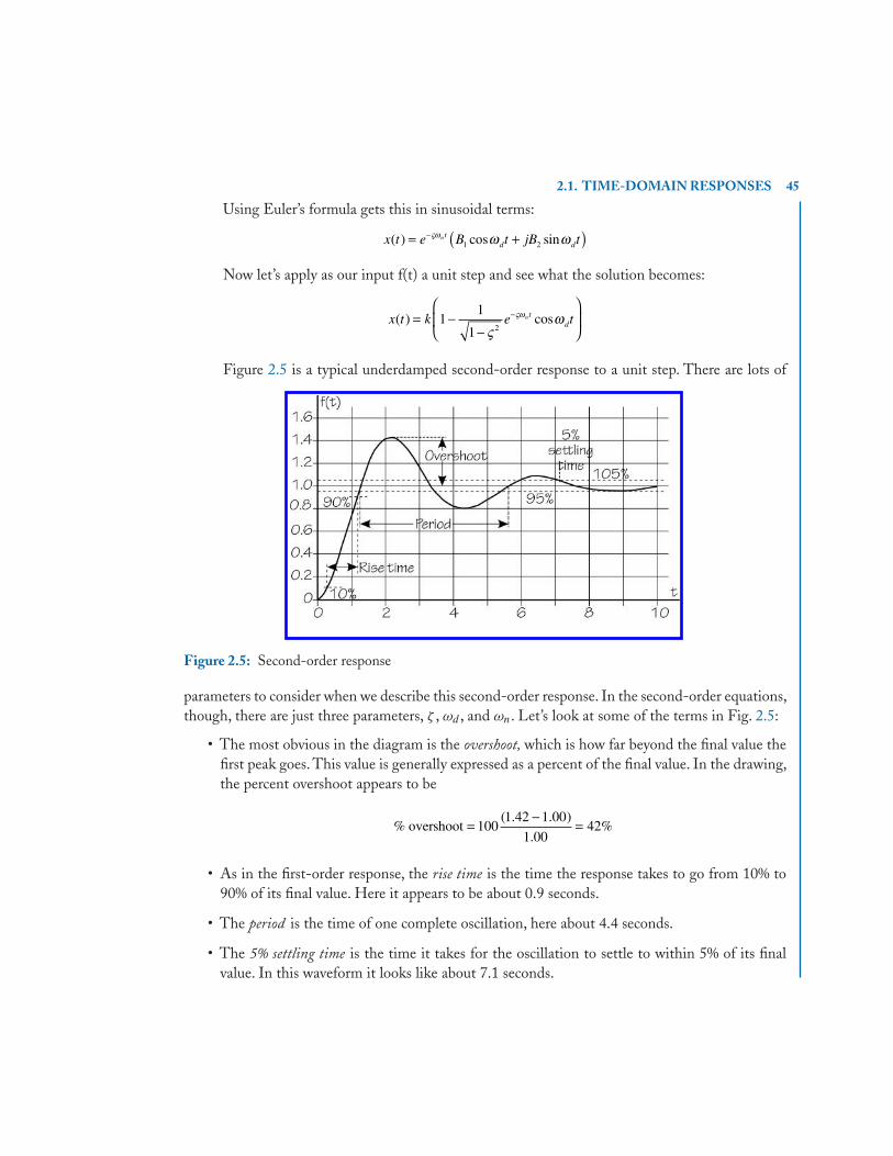
2.1. TIME-DOMAIN RESPONSES 45
Using Euler’s formula gets this in sinusoidal terms:
x t e B t jB tntd d( ) cos sin= +( )−ςω ω ω1 2
Now let’s apply as our input f(t) a unit step and see what the solution becomes:
x t k e tntd( ) cos= −
−
⎛
⎝⎜
⎞
⎠⎟−1
1
1 2ςωςω
Figure 2.5 is a typical underdamped second-order response to a unit step. There are lots of
Figure 2.5: Second-order response
parameters to consider when we describe this second-order response. In the second-order equations,though, there are just three parameters, ζ , ωd , and ωn. Let’s look at some of the terms in Fig. 2.5:
• The most obvious in the diagram is the overshoot, which is how far beyond the final value thefirst peak goes. This value is generally expressed as a percent of the final value. In the drawing,the percent overshoot appears to be
% overshoot =−
=1001 42 1 00
1 0042
( . . )
.%
• As in the first-order response, the rise time is the time the response takes to go from 10% to90% of its final value. Here it appears to be about 0.9 seconds.
• The period is the time of one complete oscillation, here about 4.4 seconds.
• The 5% settling time is the time it takes for the oscillation to settle to within 5% of its finalvalue. In this waveform it looks like about 7.1 seconds.

46 2. CHARACTERIZING A SYSTEM
We will be using these measurements from waveforms to characterize second-order systemsin the next section.
2.2 CHARACTERIZINGTime to characterize! Yes, now! Here in public! In broad daylight, no less!
Characterizing really isn’t that spectacular, and probably doesn’t even border on exciting.Whatit means is finding the parameters of the differential equation that describes the system. For a first-order system, it means finding the time constant τ . For a second-order system, the undamped naturalfrequency ωn and the damping ratio ζ
We do this by eliciting a step response of the system, which means we have to drive the systemwith a step input and see what happens. This “see” part will often be via sensors that display theoutcome on an oscilloscope.
In the examples that follow, I’m going to assume that each system is linear, that it has beenhit by a step input, and that we see the response as a trace on a carefully-adjusted scope so that theresponse fills the screen.
2.2.1 EXAMPLE I— 1st -ORDER SYSTEMWe’ve applied the step input to our system and the scope now shows the exponential response inFig. 2.6. What’s this second exponential that’s upside down? In this case, we’ve used a square wave
Figure 2.6: Example I: Scope before adjustments
to excite the system, which repeats itself—we are seeing the beginning of the second half of thatrepetition.

2.2. CHARACTERIZING 47
When making scope measurements, though, we need to pay attention to scope settings. Inorder to get the best precision, we need to use the full scope screen for our measurements, or as muchof it as we can. This means adjusting both the vertical and horizontal gains on the scope to fill thescreen with the “most measurable” trace.
Figure 2.7 is the result of this. I’ve made three adjustments:
Figure 2.7: Example I: Scope with T measurement
• The trace now begins in the lower left corner.
• The flattening exponential “lands” along the top of the scope.
• The exponential is expanded horizontally so that only part of the waveform is shown—justenough to be sure of the “landing.”
When we finish these adjustments, we read the screen calibrations: vertical 0.5V/�, horizontal10 ms/�.
We’ll calculate τ by measuring the time to the 1/e point on the trace. We learned in Sec-tion 2.1.1 that this point on a trace that is going up like this one does is at 0.632 of the full rangeand that 5/8 is a 1% approximation to that.
The trace starts in the lower left corner and fills the screen, “landing” at the top. So the tracecovers eight squares. We’ll read the time where the trace crosses the top of the fifth square. InFig. 2.7, that looks to me like 1.9 squares from the left. At 10 ms/�, that’s 19 ms, so for this system,τ = 19 ms.
The trace covers eight squares, which is 4.0 volts. The input step was a unit step (i.e., 1 volt),so the d-c gain is 4.

48 2. CHARACTERIZING A SYSTEM
The characteristic polynomial for our system is
19 10 13× +− s
and the differential equation becomes
19 10 43× + =− dx
dtx f t( )
and the transfer function is
TF sX s
F s s( )
( )
( )= =
× +−
4
19 10 13
That’s all we need to do to characterize a linear first-order system.
2.2.2 EXAMPLE II—2nd-ORDER SYSTEMThe second-order response to a unit step is more complex and so characterization is, too. We can’tget the desired parameters (ζ and ωn) directly. Also, the clarity of the “wiggles” of the second-orderresponse determines which of two methods we use. We’ll look at both here.
The scope picture in Fig. 2.8 is the result of a step of 1 volt, and the scope has been adjusted sothe picture is “good,” meaning that it fills most of the screen and there are only about two oscillationsshown. After these adjustments, the vertical calibration is 0.5 V/� and the horizontal calibration is100 ms/�.
Figure 2.8: Example II: Using log decrement

2.2. CHARACTERIZING 49
This scope trace shows two clear upward “wiggles” and we can clearly read their heights abovethe final value of the trace. Since we can read these, we’ll use the method of logarithmic decrement.(If the second one isn’t clearly readable, we have to use the second method.)
From the scope (Fig. 2.8) we collect three pieces of data:
• Height of the first peak above the final value: x1 = 2.1 squares
• Height of the second peak: x2 = 0.5 squares
• PeriodTd measured between peaks or between same-direction zero crossings:Td = 4.3 squares
That’s all the data we need to find the two parameters of this second-order system.Start by finding the logarithmic decrement. Since this is a ratio, we don’t need the actual scope
calibration, just the numbers of squares:
δ =⎛⎝⎜
⎞⎠⎟= ⎛
⎝⎜⎞⎠⎟=ln ln
.
..
x
x1
2
2 1
0 51 435
From this logarithmic decrement we get the damping ratio:
ςπδ
π=
+=
+=
1
14
1
14
1 435
0 2232
2
2
2.
.
The period that we measured is that of the damped response. The scope shows 4.3 squares at100 ms/�, so the damped period is Td = 430 ms. From this we get the damped natural frequency:
ω π πd
dT= =
×=−
2 2
430 1014 6
3. rad/s
Now we can find the undamped natural frequency:
ω ως
nd=−
=−
=1
14 6
1 0 22315 0
2 2
.
.. rad/s
Finally, we can find the d-c constant k by noting that the input is a unit step, the final valueis five squares up from the beginning. Since the scope calibration is 0.5 V/�. k = 2.5.
Remember the characteristic polynomial and the differential equation for a second-ordersystem?
ss
d x t
dt
dx t
dtx t kf
n n
n n
2
2
2
2
2
21
1 2
ως
ω
ως
ω
+ +
+ + =( ) ( )
( ) (tt)

50 2. CHARACTERIZING A SYSTEM
We have all of the numbers for these:
ss
s s
2
2
3 2 3
15 0
2 0 223
15 01
4 44 10 29 7 10.
.
.. .
+ ( ) +
= × + × +− − 11
4 44 10 29 7 10 2 532
23.
( ).
( )( ) .× + × + =− −d x t
dt
dx t
dtx t f (( )t
What happens if we can’t reliably read the height of the second peak? If there’s fairly heavydamping, this peak is often very small. Let’s use the same waveform we just worked on, but let’sassume we can’t read the second peak. This will lead to the method of fractional overshoot.
The fraction in fractional overshoot is the ratio of the height of the first peak to the distancefrom the starting point to the final value. Note: This works only for a step input.
From the graph, xo = 5 squares and xp = 2.1 squares. The fractional overshoot is
OSx
xp
o
= = =2 1
50 42
..
This yields the damping ratio
ςπ π
=+
=+
=1
1
1
10 42
0 2662
2
2
2(ln ) (ln . )
.
OS
That’s about what we got before.I’ll admit I am carrying excess precision,especially consideringthat the data from the scope are good to only about two significant digits.
Sometimes we can’t read a full period from the scope, either. In these cases, we can use thehalf period as shown in Fig. 2.9. On this trace, the half period Td/2 = 2.1 squares, which is 210 ms.The damped natural frequency becomes
ω π πd
dT= ( ) = ×
=−2 210 1015 0
3. rad/s
Again, not too bad considering that we don’t have great precision from the scope data. Thecharacteristic polynomial and the differential equation for this system are about the same as before.
One additional quantity that is often used to describe a second-order system is the settlingtime. This is the time it takes for the oscillation to settle to within a certain percentage of its finalvalue. Not uncommon are the 2% and the 1% settling times:
2% settling time
1% settling time
.
.
=
=
3 9
4 6
ςω
ςω
n
nn
For our example (using the logarithmic decrement data), these are 1.2 s and 1.2 s.
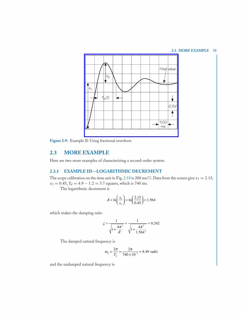
2.3. MORE EXAMPLE 51
Figure 2.9: Example II: Using fractional overshoot
2.3 MORE EXAMPLEHere are two more examples of characterizing a second-order system.
2.3.1 EXAMPLE III—LOGARITHMIC DECREMENTThe scope calibration on the time axis in Fig. 2.10 is 200 ms/�. Data from the screen give x1 = 2.15,x2 = 0.45, Td = 4.9 − 1.2 = 3.7 squares, which is 740 ms.
The logarithmic decrement is
δ =⎛⎝⎜
⎞⎠⎟= ⎛
⎝⎜⎞⎠⎟=ln ln
.
..
x
x1
2
2 15
0 451 564
which makes the damping ratio
ςπδ
π=
+=
+=
1
14
1
14
1 564
0 2422
2
2
2.
.
The damped natural frequency is
ω π πd
dT= =
×=−
2 2
740 108 49
3. rad/s
and the undamped natural frequency is

52 2. CHARACTERIZING A SYSTEM
Figure 2.10: Example III
ω ως
nd=−
=−
=1
8 49
1 0 2428 75
2 2
.
.. rad/s
The characteristic polynomial for Example I is
ss
s s
2
2
3 2 3
8 75
2 0 242
8 751
13 1 10 55 3 10.
.
.. .
+ ( ) +
= × + × +− − 11
2.3.2 EXAMPLE IV—FRACTIONAL OVERSHOOTIn Fig. 2.11, the time axis calibration is 0.5 s/�. Data from this response have to be taken forfractional overshoot because the second peak is hard to measure. The results are xo = 5, xp = 1.5,and Td/2 = 2.0 squares, which is 1.0 seconds.
Using the fractional overshoot
OSx
xp
o
= = =1 5
50 30
..
makes the damping ratio
ςπ π
=+
=+
=1
1
1
10 30
0 3582
2
2
2(ln ) (ln . )
.
OS

2.4. SUMMARY 53
Figure 2.11: Example IV
The damped natural frequency is
ω π πd
dT= ( ) = =
2 1 03 14
.. rad/s
and the undamped natural frequency is
ω ως
nd=−
=−
=1
3 14
1 0 3583 36
2 2
.
.. rad/s
2.4 SUMMARY
This chapter has been about “getting the numbers” from the response of a system. When we have areal, physical system and need to describe it mathematically, probably for designing a controller forthe system, we need some clues as to how the system responds.
We’ve done just linear first- and second-order systems. The techniques here can be expandedto higher-order systems, which gets messy, and to non-linear systems, which gets even messier. Bothof these are beyond what we are doing in this course.
I’ve chosen to use a step to excite these systems. We can also get the response by using asinusoidal input, but that, too, is beyond our scope here.
Note that the outcome is the characteristic polynomial, which in the s domain completelydescribes the response of a linear system and therefore its transfer function. Since we generally design

54 2. CHARACTERIZING A SYSTEM
closed-loop control systems in the s domain, this characteristic is just what we need for the devicewe plan to control.

FORMULAS AND EQUATIONS 55
FORMULAS AND EQUATIONS1. First-order linear system and s-domain solution.
ττ
τ
dx t
dtx t kf t X s
kF s
strise
( )( ) ( ), ( )
( )
.
+ = =+
=1
2 2
2. Second-order linear system and s-domain solution
1 22
2
2ως
ωn n
d x t
dt
dx t
dtx t kf t X s
kF( ) ( )( ) ( ), ( )
(+ + = =
ss
ss
n n
)2
2
21
ως
ω+ +
3. Second-order system roots
s n n1 22 1
0 1
1
, = − ± −≤
=
ςω ω ςςς
< underdamped
criticallly damped
> overdampedς 1
4. Underdamped second-order system roots
s jn n d n1 22 21 1, ,= − ± − = −ςω ω ς ω ω ς
5. Characterizing using logarithmic decrement
δ ςπδ
ω π ω ως
=⎛⎝⎜
⎞⎠⎟
=+
= =−
ln ,
,
x
x
Tdd
nd
1
22
2
2
1
14
2
1
6. Characterizing using fractional overshoot
OSx
x
OS
p
o
= =+
,
(ln )
ςπ
1
12
2

56 FORMULAS AND EQUATIONS
7. Settling times
2% settling time
1% settling time
.
.
=
=
3 9
4 6
ςω
ςω
n
nn
8. % Overshoot from damping ratio
%OS e=−
−100 1 2ς π
ς

57
C H A P T E R 3
InstrumentationInstrumentation—putting instruments into a system. Of course, there are all kinds of instruments,trombones, scalpels, even screwdrivers. Here, though—electrical instruments. Why electrical? Be-cause we usually want a “reading” of a physical parameter some distance away from where theparameter is actually “happening.”
A simple example of electrical instrumentation is the thermostat that controls the heat inyour house. The device uses the thermal expansion of metal to detect changes in temperature. Themovement of that metal is converted to an off-or-on electrical signal by a set of contacts. Thiselectrical signal is delivered to the furnace to control the gas valve or the heat pump.
In this chapter I’m going to stick with just a couple of different physical quantities to be“read,” strain and temperature. But before that, let’s look at how we can use electrical informationto determine the value of a physical quantity as precisely as possible.
Many instruments alter a voltage or a current associated with the parameters they sense. Thatalteration may be very small, sometimes only a few percent. So we are faced with reading a smallchange and we want to read this change as precisely as we can.
Let’s presume that our gauge, whatever it is, has to operate on 10 volts. As the physicalparameter is changed, that voltage is raised or lowered in a linear manner. Suppose the largestexpected change is 4%, which means the voltage actually ranges from 9.6 to 10.4 volts. For myexample, I’m going to read this using a digital voltmeter.
Now suppose I want to measure this parameter to a precision of one part in a thousand, 0.1%.At the maximum expected parameter value, the voltage is 10.4 V. I want to detect a 0.1% change,so I must be able to observe a change in the parameter from 4% to 4.004%. This means I need to beable to read a voltage of 10.4004 volts. To do this, I must have a voltmeter that is precise to aboutsix significant digits. Not unheard of, but expensive.
Let’s get clever and build a circuit that somehow precisely subtracts that “base voltage” of 10volts from the gauge’s signal. The circuit that does this subtraction must be precise and stable, but itturns out this is not hard to do.
After I precisely subtract 10 volts, the range of the change of voltage from the gauge is −0.4to +0.4 volts. At the +0.4 V end, 0.1% means at most 0.4004 VV, a precision of just four significantdigits. That’s not as hard to do as the original six. In the next section we’ll see how a Wheatstonebridge does this “subtracting.”

58 3. INSTRUMENTATION
3.1 STRAIN GAUGE
The resistance strain gauge is simple, precise, and inexpensive. It measures strain, usually statedin percent elongation. It works by stretching or compressing a conductor whose dimensions arecarefully controlled. Figure 3.1 shows how the conductor is laid out on the substrate. Figure 3.2shows the size of a typical gauge.
Figure 3.1: Strain gauge
Figure 3.2: Strain gauge
The electrical parameter that changes with strain is the resistance of the conductor.The changein resistance is directly proportional to the strain the gauge undergoes. To use the gauge, you glue itto the surface to be tested and run wires to the metering system. Figure 3.3 shows two gauges gluedto an aluminum bar.
Gauges are not expensive. Omega sells standard strain gauges for around $50 for a pack often, for example.
The resistance of a conductor depends on three parameters, conductivity (a property of themetal the conductor is made from), length, and cross-sectional area:
RL
A=σ

3.1. STRAIN GAUGE 59
Figure 3.3: Strain gauge attached to beam
It is the length parameter that we are most concerned with. The change in length is propor-tional to strain and the change in resistance is proportional to length. Hence, the change in resistanceis proportional to strain.
There’s another effect operating here, though, that we at least have to be aware of. As theconductor lengthens, its cross-sectional area must decrease because there is a constant volume ofmetal. Increasing the length increases the resistance,but it also decreases the area,which also increasesthe resistance.This effect is a second-order effect, though, and for many measurements we can ignoreit. A check of the manufacturer’s literature will tell you how much this decrease in area affects themeasurement.
But wait! We aren’t done with “effects” yet. The strain gauge also has what is called transversesensitivity.This is a measure of how much the gauge is affected by a strain at right angles to the desiredstrain and the “long way” position of the gauge. Note in Fig. 3.1 the little sections of conductorthat run across the gauge where the conductor turns a corner. These little sections are sensitive totransverse strain, or strain across the beam. The package in Fig. 3.2 shows a transverse sensitivity of(0.4±0.2)%, which says that the resistance of the gauge is affected by this transverse strain only toat most 0.6% of the gauge’s resistance.
For a typical strain gauge, the strain, expressed in terms of the change in resistance is
ε ≈ΔR
R
where R is the unstrained resistance of the gauge.For the gauge itself, the change in resistance is

60 3. INSTRUMENTATION
ΔR G R= ε
where G is a gauge constant, ε is the strain, and R is the gauge resistance (unstrained). Gauges arecommonly made with standard values of R: 120, 240, 350, and 1,000 ohms. A common gauge factoris about 2. Note in Fig. 3.2 that the gauge factor G is 2.090±0.5% and the gauge resistance R is120.0±0.3% �
Gauges are also affected by temperature, which should be taken into account for very precisemeasurements. Omega, for example, makes gauges whose temperature coefficient is matched eitherto steel or to aluminum.
3.1.1 VOLTAGE DIVIDERI want to get from a gauge a voltage that varies with strain. The simplest circuit I can think of is thevoltage divider (Fig. 3.4), where R2 is the gauge. I’ll choose a second resistance R1 to be 120 ohms,
Figure 3.4: Strain gauge in voltage divider
equal to R2, the gauge resistance. This makes Vo = 1/2Vs for zero strain.In fact, if I want a resistor for R1 that is as precise as the gauge resistance, why not just use a
second gauge? This “other gauge” is placed so that it will not undergo any strain and hence remain120 ohms. Moreover, this “other gauge” will be affected by temperature in the same way as theactual gauge and to some extent balance out the effect of temperature change. (Gauges are prettyinexpensive.)
Now write the equation for the voltage divider:
V VR
R Ro s=+
2
1 2
Replace the gauge resistance R2 with its total resistance that includes R:
R R R R G R R G
R R
V VR G
R R
g g g g
g
o sg
g
2
1
1
1
= + = + = +=
=+
+
Δ ε ε
ε
( )
( )
ggsG
VG
G( )1
1
2+=
++ε
εε

3.1. STRAIN GAUGE 61
Suppose that the gauge factor G is 2.00 and the supply voltage Vs = 5.0000 V. For zero strain,Vo = 2.5000. For 1% strain:
Vo1 51 0 02
2 0 022 524752=
++
=.
.. V
Suppose we want to read the strain to a precision of 0.001. If the strain is 1.001%, the voltageVo will be
V Vo1oo1 =++
=51 0 02002
2 0 020022 524777
.
..
Precision of 0.001 is a voltage difference of only 0.000025 V, which is 25 microvolts. Thevoltmeter must be precise to six digits after the point, seven digits total.
3.1.2 WHEATSTONE BRIDGEMy voltage-divider example shows that it would be very nice if we could somehow subtract outthe zero-strain voltage. In the example, the zero-strain voltage was 2.50000 V, while the voltagefor 1% strain was 2.524752 V. If we could somehow subtract 2.5 volts, the 1% strain would read0.024752 volts.We could amplify this by, say, a factor of 100 so the voltmeter would read 2.4752 volts.Now a precision of 0.001 requires only that the voltage be read ± 0.0025 volts, which is 2.5 millivolts.That requires only four digits after the point in our voltmeter.
The Wheatstone bridge was invented in 1833 by … no, not Sir Charles Wheatstone (1802–1875) but by Samuel Christie. It implements a concept sometimes called differential measurement.This circuit balances out the zero-strain voltage and gives a reading of just the voltage associatedwith the strain itself. The bridge in Fig. 3.5 has two strain gauges and two resistors in it. The twostrain gauges are in the upper arms; the two resistors are in the lower arms.
Figure 3.5: Strain-gauge bridge—two arms

62 3. INSTRUMENTATION
A clever part of this circuit is in the placement of the strain gauges on the beam being stressed.One gauge, on the upper left, is attached to the bottom of the beam; the other gauge, on the upperright, is attached to the top of the beam. If the beam is being deflected downward, the top gauge(upper right arm) sees tension and positive strain while the bottom gauge (upper left arm) seescompression and negative strain. This doubles the sensitivity of the measurement.
The two resistors in the lower arms of the bridge are precision resistors whose resistance isidentical to that of the strain gauges. If for example we use 120-� gauges, the bottom resistors willbe 120 � also.
Analysis of this bridge circuit is done using the voltage-divider relationship. But rememberthat a voltage divider is a valid method only when the divider doesn’t “leak,” meaning that there is nocurrent being drawn from the divider itself. That’s the situation here because we are going to put avoltmeter between the middle terminals of the bridge. That meter will draw only a very tiny currentfrom the terminals (microamperes) and will barely affect the voltage dividers. Moreover, we willfind that when the bridge is exactly balanced, i.e., all four resistances are exactly equal, the voltagebetween the terminals will be zero.
Let’s start the analysis. The voltages referenced to ground at the plus and the minus terminalsare
V VR
R RV V
R
R Rsgb
sgt
+ −=+
=+
1
1
1
1
,
Now apply the strain gauge equations
R R G R R R G R
R Rgb g g gt g g
g
= − = +=
ε ε,
1
The two signs account for the fact that the bottom gauge is compressed when the beam ispressed downward, while the upper gauge is stretched.
The voltmeter reads the difference:
V V V VR
R R G R
R
R R G R
V
o sg
g g g
g
g g g
s
= − =+ −
−+ +
⎡
⎣⎢⎢
⎤
⎦⎥⎥
=
+ − ε ε
11
2
1
2
2
4 2 2−−
+⎡⎣⎢
⎤⎦⎥=
−G GV
G
Gsε εεε
If the strain is no more than 0.04, then G2ε2 is no more than 0.0064 for a gauge factor G = 2.If G2ε2 � 4, the voltage formula becomes
for 12
, VVGo
s=
When the strain is zero, so is Vo. For Vs = 5.0 V, G = 2 and ε = 1%, the bridge voltageVo = 0.05 V, a voltage that within the range of any decent digital voltmeter.

3.1. STRAIN GAUGE 63
3.1.3 IMPROVED BRIDGEIn the previous example, the two gauges were in the upper arms of the bridge. One was attachedto the tension side of the beam; the other, to the compression side. We could use for the two lowerarms two more gauges but unattached to the beam. This isn’t a bad idea for several reasons: gaugesare cheap, they provide exactly the right resistance, and they give all four arms the same temperaturecoefficient.
Hmmmm, since we have two unstressed gauges, could they be attached to the beam as well?Yup! We’ll attach all four gauges to the beam, two on the top and two on the bottom (Fig. 3.6). The
Figure 3.6: Strain-gauge bridge—four arms
gauges on the same side of the beam are in diagonally opposite arms of the bridge. The photo inFig. 3.3 shows two gauges on top of a beam. The other two are not visible underneath.
The analysis of the circuit of Fig. 3.6 proceeds as before.
V VR
R R
R
R R
R R G R
o sgt
gb gt
gb
gb gt
gt g g
=+
−+
⎡
⎣⎢⎢
⎤
⎦⎥⎥
= + ε ,
( ) (
R R G R
R R R
V VR G
R
R
gb g g
gt gb g
o sg
g
g
= −+ =
=+
−−
ε
ε
2
1
2
1 GG
R
VG
V V G
g
s
o s
εε
ε
)
2 22
⎡
⎣⎢⎢
⎤
⎦⎥⎥=
=
The outcome is a measurement that is twice as sensitive as the two-arm bridge.There’s one more adjustment that we need to make, though. I have been assuming all through
this bridge stuff that the four arms of the bridge are, in their unstressed state, exactly equal. I needthis to be true so that the bridge voltage Vo is exactly zero for zero stress. But alas, that’s not always

64 3. INSTRUMENTATION
going to be 100% true, so we need a way to make a minor adjustment to the bridge. Figure 3.7 showsone way of doing this.
Figure 3.7: Bridge adjustment
The added resistance between the two left arms of the bridge is an adjustable resistor. Oncethe gauges and the bridge are set up and before any gauges are stressed, the adjustable resistance,called a “pot,” (short for potentiometer), is adjusted by moving the tap (the arrow in the drawing)up or down until the voltmeter reads exactly zero. Then the bridge is ready to read strain via thevoltmeter readings.
3.1.4 EXAMPLE I–2-ARM STRAIN-GAUGE BRIDGETwo strain gauges (R = 120�, G = 2.090) are set up in the two-arm bridge arrangement of Fig. 3.5.The bridge supply is Vs = 5.0 V. The voltmeter reads Vo = 86.213 mV. Find the strain in percent.
For the two-arm bridge, the voltage relationship is
VV
Gos=
2ε
For the data given,
86 213 105
22 0903. .× =− ε
so
ε = 1 65. %

3.2. RESISTANCE TEMPERATURE DETECTOR 65
3.1.5 EXAMPLE II–4-ARM STRAIN-GAUGE BRIDGEFour gauges (R = 120 �, G = 2.090) are set up in a four-arm bridge arrangement of Fig. 3.6. Thesupply voltage is 5.0 V and the voltmeter reads Vo = 86.213 mV. What is the indicated strain?
For the four-arm bridge,
V V Go s= ε
The result is
86 213 10 5 2 090
0 825
3. ( )( . )
. %
× ==
− εε
Note that this four-arm bridge is twice as sensitive as the two-arm bridge.
3.2 RESISTANCE TEMPERATURE DETECTORThere are lots of common ways to measure temperature, or I suppose I really should say, to sensetemperature. Different sensors have different properties:
Thermometer: Changing volume, very common, inexpensive, hard to “electrify” for a controlsystem
Thermocouple: Self-generated voltage, very inexpensive, covers wide range of temperature,small, but requires reference junction
Integrated circuit: Transistor-like element varies current, inexpensive, generally linear withtemperature, rugged, sensitive
Thermistor: Varying resistance, rather fragile, narrow range
Resistance temperature detector: Varying resistance, precision sensor, stable and accurate, expen-sive
In this section we are going to examine the resistance temperature detector because it is arugged sensor designed to be used in a variety of situations. We apply the Wheatstone bridge as wedid with strain gauges. Later we’ll look at thermocouples because they are used in a manner that isvery different from the resistance temperature detector.
3.2.1 RTD ITSELFThe RTD (one gets tired of saying the whole name!) is a standardized resistance with a very pre-dictable and repeatable temperature characteristic. One popular type is a platinum resistance with a0˚C resistance of 100 ohms. (See Fig. 3.8.) The resistor itself often has four wires connected ratherthan two.

66 3. INSTRUMENTATION
Figure 3.8: RTD
The sensor can be obtained in different “packages,” depending on the application. Fig. 3.9shows a model with the resistive element encased in a stainless steel tube. The resistance element isat the tip of the tube.
Figure 3.9: Resistance temperature detector
The resistance of the gauge Rg varies in a fairly friendly way with temperature. The actualrelationship is a power series, the first terms of which are the Callendar–VanDusen equation:
R R T T
T C
g o= + × − ×( )≤ ≤ °
− −1 3 9083 10 5 775 10
0 850
3 7 2. .
for T < 0˚C , the equation is different (different coefficients and a T3 term).We often use an “official” linear equation with a DIN-standard coefficient, now the official
International Electrotechnical Commission (IEC) standard:
R Tg = +100 1 0 00385( . ) for T in °C
The error between this linear equation and the polynomial is 0.007% at 100˚C, 0.648% at 200˚C, and 2.805% at 400˚C. We’ll use the linear standard in the examples.
3.2.2 2-WIRE RTD BRIDGEUsing the RTD in an instrumentation system is a lot like using a strain gauge. We’ll use a bridgejust as we did with the strain gauge. But there’s a major difference—the RTD is expensive ($100) sothere will be just one of them in the bridge. (Besides, think about how one might deploy four RTDslike we did strain gauges!)
Figure 3.10 is the “2-wire” bridge circuit; i.e., two wires connecting the RTD. The threeresistor arms are chosen to be exactly 100 �. We could also include a pot in the left corner just aswe did for adjusting the strain gauge bridge (Fig. 3.7), but I won’t do that here.

3.2. RESISTANCE TEMPERATURE DETECTOR 67
Figure 3.10: RTD 2-wire bridge
The complication is that the RTD’s connecting wires have resistance that cannot be ignored.For example, if the two wires add just one ohm total, their effect is to make the indicated temperatureappear to be 2.6˚C higher.
Analysis is the same as with the strain gauge. There are two voltage dividers and Vo is thedifference between the voltages of the two dividers. The wire resistance Rw is present twice in theupper right arm. The voltmeter draws essentially no current.
The two voltage divider equations are
V V V VR Ro s o s
g w+ = =
+ +1
2
100
100 2, –
Combining these and simplifying gives us the 2-wire bridge equation:
V V V VT R
T Ro o o sw
w
= − =+
+ ++ −0 385 2
400 0 77 4
.
.
To be able to make a calculation of temperature T from a reading of the voltage Vo, we needto know the wire resistance Rw, but this can generally be measured after installation of the sensor.
3.2.3 3-WIRE RTD BRIDGERemember the two extra wires on the RTD in the drawing of Fig. 3.8? Those two extra wires comein handy for both the three-wire bridge and the four-wire ohmmeter.
Figure 3.11 shows the “three-wire” bridge arrangement; i.e., three wires connecting the RTD.Notice that the Vo− terminal is connected to one of the extra wires, not to the right-hand corner ofthe bridge. Now consider why.
The voltmeter draws essentially zero current, so the current through the wire resistance of thisthird wire is zero—or very close to it. Hence, there is no voltage drop along that wire. While this

68 3. INSTRUMENTATION
Figure 3.11: RTD 3-wire bridge
sounds like it might balance out all wire resistance, it doesn’t, as the following equations show. I’mgoing to get Vo in terms of T in the same way I did it for the two-wire bridge. This time, there is anRw in both the upper and lower arms on the right.
V V V VR
R R
V V V V
o s o sw
g w
o o o s
+
+ −
= =+
+ +
= − =
1
2
100
100 2
0
, –
..
.
385
400 0 77 4
T
T Rw+ +
The difference between this and the two-wire equation doesn’t seem to be much. Here, thenumerator has no 2Rw term. This has the effect of cancelling out some but not all of the effects ofthe wire resistance.
Why didn’t we have this wire-resistance problem with strain gauges? Because in the four-armstrain-gauge bridge, all the wire resistances balance out.
3.2.4 COMPARISON OF TWO BRIDGESLet’s compare the two bridge methods for reading an RTD. For something to work with, I’ll use asupply voltage Vs = 10 V and assume the temperature T = 20 ˚C.
I’ll start with no wire resistance, so putting Rw = 0 in each of the equations gives the “perfect”result:
V20 100 385 20
400 0 77 20185 36=
+=
( . )( )
( . )( ). mV
Now make the wire resistance Rw = 0.1 �. For the two-wire bridge:
V20 100 385 20 2 0 1
400 0 77 20 4 0=
++ +
( . )( ) ( )( . )
( . )( ) ( )( .11190 00
).= mV

3.2. RESISTANCE TEMPERATURE DETECTOR 69
For the three-wire bridge:
V20 100 385 20
400 0 77 20 4 0 1185 19=
+ +=
( . )( )
( . )( ) ( )( . ). mV
The result is that the two-wire bridge gives a result 2.50% larger than the “perfect” value,while the three-wire bridge gives a result that is 0.09% less.
3.2.5 4-WIRE OHMMETERWould you believe there’s still one more configuration—and it completely eliminates the wire resis-tances? So you might just wonder why we even bothered with the bridge circuits. The reason is thatthis final method tends to be more expensive.
The circuit for the four-wire ohmmeter is Fig. 3.12. It works as follows:
Figure 3.12: RTD 4-wire ohmmeter
• The current source Is is precise, which means that its value is known and constant.
• The voltmeter is connected through the other pair of wires. It draws essentially no currentthrough those wire resistances, so the voltage it measures is the actual voltage across the gaugeresistance Rg .
• The current Is flows through the RTD. None of it goes to the voltmeter.
• Since all of the current Is flows through the gauge resistance Rg and the voltmeter trulyindicates the voltage across Rg , the result is
V I R I Tm s g s= = +( )( )( . )100 1 0 00385
From this formula we can get T directly.

70 3. INSTRUMENTATION
3.2.6 EMPLOYING AN RTDYou can’t just stick an RTD into a tank or a pipe or a duct and expect perfect performance. So whatshould you think about? Several things come to mind:
• Immersion in the fluid so that the RTD is truly “seeing” the temperature and isn’t in somekind of pocket
• Wiring that is as immune as possible from outside electrical interference (Chapter 5)
• Current through the RTD chosen so that the RTD is not self-heating, meaning that thecurrent is not heating the resistance element enough to give a false temperature reading
Consider the last one for a moment. In my comparison of the two bridge methods (Sec. 3.2.4),I chose a bridge supply voltage Vs = 10 V. In both bridge circuits (Figs. 3.10 and 3.11), this voltagedrives both voltage dividers. Ignore wire resistance for the moment.The current through each bridgearm is
iarm =+
=10
100 10050 mA
This current heats the RTD by plain ordinary i2R heating:
P iRTD arm= =100 0 252 . W
The hard question is, is this too much heat? The answer is, it depends! If the RTD is ingood thermal contact with a large thermal mass that it’s sensing, maybe this is OK. This is simplysomething that you need to watch out for.
Notice that if I had chosen a bridge supply of just one volt, the current would be one-tenthas large and the heating would be one-hundredth as large—just 2.5 mW.
3.2.7 EXAMPLE III–COMPARING RTD CONNECTIONSAn RTD is connected using two different bridge connections, one at a time. The wire resistance forboth is Rw = 0.2 �. In keeping with what I just said about self-heating, I’m setting the power supplyto Vs = 1 V. In each case, the voltage reading is 80.000 mV. What temperature is being sensed?
The equation for the two-wire bridge with the numbers filled in is
0 08 10 385 2 0 2
400 0 77 4 0 2.
. ( )( . )
. ( )( . )=
++ +
T
T
which when solved for temperature T gives
T C= °97 910.
Doing the same things with the three-wire bridge gives a slightly different result:

3.3. THERMOCOUPLE 71
0 08 10 385
400 0 77 4 0 2
99 147
..
. ( )( . )
.
=+ +
= °
T
T
T C
Which one is right? The simple answer is, Yes! Yes, they are both right; no, they aren’t. Themeter is reading a particular voltage, namely, 80 mV.The outcome is affected by the choice of bridge.
What happens when we think a little differently? Suppose the actual temperature has beencorrectly sensed by the two-wire bridge. If we change to a three-wire bridge, what voltage does ourmeter read:
V
V
o = + +1
0 385 97 910
400 0 77 97 910 4 0 2
( . )( . )
( . )( . ) ( )( . )
oo = 79 160. mV
The wiring makes a difference!
3.2.8 EXAMPLE IV–RTD OHMMETERSuppose the actual temperature is the value we just found using the two-wire bridge: T = 97.910˚C.What voltage do we get from the four-wire ohmmeter measurement?
I’m going to choose a current Is = 5 mA because that’s what the current was in both of theprevious examples (1 volt divided by 200 ohms). Here is the calculation:
V I R
Vm s g
m
= = × + ×=
−( )( )( . . )
.
5 10 100 1 0 00385 97 910
688 4
3
88 mV
This method gives a much higher voltage to observe on the voltmeter for the same amountof self-heating.
3.3 THERMOCOUPLE
Thermocouples are great! They are so-o-o-o simple. Just twist together a couple of wires made ofdifferent metals and you’ll get a voltage that is very predictably related to the temperature of thejunction. Golly, what could be neater?
But wait! If you twist together two wires of differing metals, you’ll have to join two wires ofdiffering metals somewhere else in the circuit as well. Otherwise, you won’t have a closed loop. Noloop, no circuit. Thermocouples are simple but you can’t build a single junction into a circuit.
3.3.1 SEEBECK EFFECTThomas Johann Seebeck (1770–1831) discovered the effect that bears his name. It says that if youmake a junction of two dissimilar metals and heat the junction, you’ll get a voltage. This isn’t a

72 3. INSTRUMENTATION
big voltage, typically something in the neighborhood of 40 μV/˚C, so even 1,000˚C will yield only40 mV. But there’s a voltage nevertheless.
Figure 3.13 shows this simple arrangement. The voltage produced depends on what metalsyou choose for the wires and it depends on the temperature. The relationship between voltage andtemperature isn’t linear, either. The polynomial relationships between voltage and temperatures forvarious combinations of metals are well documented.
Figure 3.13: Seebeck effect
But as I said, you can’t have a junction of two dissimilar metals without a second junction.Figure 3.14 shows one arrangement with two different metals, a voltmeter with copper terminals,and a ice-water bath for a constant 0˚C for the second junction. The strange names are specializedalloys made for thermocouples. (See Fig. 3.18.)
Figure 3.14: Thermocouple system I
The second junction J2 is called the reference junction because it provides the base temperatureto which the temperature of the junction J1 is referenced. The measured voltage is therefore causedby the difference in temperature between the heated junction and the 0˚C reference junction.
This reference could be at any fixed, stable temperature, not just 0˚C. If we choose some otherreference, then the voltage represents the temperature difference between the two. If, for example,we have a well-regulated oven at exactly 27˚C, then the voltage is related to T – 27.

3.3. THERMOCOUPLE 73
3.3.2 OTHER JUNCTION ARRANGEMENTSIce water is pretty inconvenient as a permanent feature of a temperature-measuring system, so weoften use a block of material that can be kept by some means at a constant temperature. This blockis called an isothermal block because its temperature is the same all over the block.
Figure 3.15 uses such a block to keep the two copper terminals of the voltmeter cable at thesame temperature. The purposes of this is to control any small temperature difference between thevoltmeter cable connections. The second junction J2 is still in the ice-water bath.
Figure 3.16 expands the block to include the second junction. The thinking here is that theblock is being held at a constant temperature for the cable connections, so why not use it for thereference as well.
Figure 3.15: Thermocouple system II Figure 3.16: Thermocouple system III
Figure 3.17 goes to the ultimate and just lets the voltmeter cable terminate both of the metalsof the thermocouple. In this arrangement and in the previous one, the block is providing the referencetemperature.
Figure 3.17: Thermocouple system IV
Any way you do it, you still have to maintain a second junction at a steady reference temper-ature. Now, what can go wrong with this simple arrangement? Here are a few problems:

74 3. INSTRUMENTATION
• Bad connections, which interfere with the current from the very small junction voltages
• Wrong extension cables that create extra but uncontrolled junctions (there are cables designedfor use in thermocouple circuits)
• Lead resistance, which means the meter current must be kept very low
• Junction diffusion, whereby at higher temperatures, one metal diffuses into the other, decali-brating the junction
• Noise insertion on the cable, interfering with the small junction voltages (Example III inChapter 5).
3.3.3 THERMOCOUPLE TYPESThere are many different metal combinations that can be used to build thermocouples. All of themtake two dissimilar metals and make two junctions, one to sense the temperature and the other tobe the reference. Over the years, various strange-sounding alloys have been developed for thermo-couples.
I’m going to show four fairly common types of thermocouples. The table of Fig. 3.18 lists thecharacteristics of Types E, J, K, and T. I’ve ignored those that use platinum alloys such as Types B,R, and S.
Figure 3.18: Some thermocouple types
Each of these types is described by a power series, the coefficients of which are well docu-mented. All the polynomials are of the form
ΔT a Vi si
i
n
==∑
0

3.4. MORE EXAMPLE 75
where the coefficients are those of Fig. 3.19. The voltage Vs is the observed Seebeck voltagein microvolts, and T is the temperature difference between the junctions in Celsius.
Figure 3.19: NIST thermocouple polynomial coefficients
If you need to employ thermocouples, a most important facet of your job is to pay closeattention to metals and junctions, especially unwanted or uncontrolled ones.
3.4 MORE EXAMPLE
3.4.1 EXAMPLE V–BROKEN STRAIN-GAUGE BRIDGEFour strain gauges (R = 120 �, G = 2.090) are connected in a four-arm bridge (Fig. 3.6). Thepower supply Vs = 5.0 V. The voltmeter is presently reading Vo = 0.15675 V.
The gauge in the upper right arm of the bridge fails open (see Fig. 3.20). In other words, thegauge is replaced by an open circuit. What does the voltmeter read now?
Figure 3.20: Bridge with broken arm

76 3. INSTRUMENTATION
Remember that the voltmeter draws a very small current, small enough that the current doesn’taffect the bridge. The meter’s minus lead is still connected to the right corner of the bridge. Now,though, that right corner has only one gauge connected to it, the gauge in the lower right arm. Theother gauge has become an open circuit.
The voltmeter’s current is so small that there is negligible voltage drop across that lonely gaugeon the lower right. Therefore, the voltage of the minus terminal is essentially that of the groundreference. So we can write
V− = 0
and therefore the voltmeter readsV V V Vo = − =+ − +
To finish this, we need the voltage V+, which is not VS/2 because the gauges are stressed. Toget this, we need to know the gauge resistances. To get the gauge resistances, we need the strain thatwas being experienced. For the unbroken four-arm bridge,
V V Go s= ε
which yields
0 15675 5 2 090
0 015
. ( )( . )
.
==
εε
Now we can find the values of the two gauges on the left:
R R G R R R G R
R Rgt g g gt g g
gt gb
= + = −= =
ε ε,
. ,123 76 1Ω 116 24. Ω
From these comes V+, which is the voltage divider on the left with resistances Rgt and Rgb:
VR
R Rgt
gt gb+ = +
=+
=
5 5123 76
116 24 123 76
2 5783
.
. .
. V
Because the voltage on the right, V is 0, the voltmeter must be reading Vo = 2.5783 V.
3.4.2 EXAMPLE VI–RTD WIRINGAn engineer you work with needs to know the wire resistance of the cable that ties an RTD to acontrol room display. The RTD is in a vat; its wires run in a standard instrumentation cable by someroute that no one can locate. The only thought is that it’s in a conduit somewhere.
To make this messier, the process that’s running cannot be stopped. That means that yourfriend cannot simply apply an ohmmeter to the cable to see what its resistance is. An ohmmetercannot be used when the circuit being checked is powered or is connected to something else.

3.4. MORE EXAMPLE 77
Your friend devises a scheme where he is going to measure the temperature at the RTD tipusing a simple thermocouple, then relate that temperature information to the voltage being read inthe control room. He builds a Type E thermocouple, welding the twisted wires to make sure theystay together. Then he insulates them with a thin plastic coating. The lead wires are long enough toreach out of the vat so the second junction can be in ice water and he can attach a precision voltmeterto the thermocouple wires.
He positions one junction in the vat very close to the RTD tip. He positions the other inice-water made with distilled water and carefully stirred to make sure the ice-water junction is trulyat 0˚C. He checks the ice water using a precision thermometer.
As he takes a reading of the thermocouple voltage, he asks the technician in the control roomto take a reading of the voltage at that end of the RTD cable. Here are his data:
• Thermocouple voltage VT = 2.1256 mV
• RTD voltage VR = 60.429 mV
• RTD supply voltage (three-arm bridge) Vs = 2.00 V
The solution requires three steps.The first is to determine the temperature being sensed by thethermocouple, which he’ll do using the NIST thermocouple polynomial for a Type E thermocoupleshown in the table of Fig.3.19.To avoid loss of precision,he’s going to work to the nearest thousandth.The polynomial is
ΔT= a Vn Tn
i
n
=∑
0
(VT must be in microvolts.)Using the numbers given in the table and the value of VT from the engineer’s measurement,
the result is
ΔT V VT T= × − × +− −1 7057035 10 2 3301759 10
6 543
2 7 2. .
. 55585 10 7 3562749 10
36 256 1 053
12 3 17 4× − ×= − +
− −V VT T.
. . 00 063 0 002
35 264
. .
.
−= °C
The second step is to write the equation for the voltage from the 3-wire bridge using thetemperature just measured and then equate this to the voltage VR observed at the bridge:
20 385 35 264
400 0 77 35 264 460 429 1
. .
. ..
( )( )+ ( )( ) + = ×
Rw
00 3−
Solving this for the wire resistance gives a value of Rw = 5.547 � per conductor.Odd approach? Perhaps. Can you think of a different way that might not be as hard to carry
out? Your goal is to obtain the resistance of the wires in the cable that connects the RTD through a

78 3. INSTRUMENTATION
3-wire bridge to the control room without disrupting operations. [Clue: There is a very simple waythat’ll make you wonder where the engineer went to college!]
Another question. These results are supposed to be to the nearest thousandth. By how muchis the final result changed if the ice-water junction is at 0.001˚C instead of 0?
3.5 SUMMARYOn the surface, this chapter is about three particular instruments, the strain gauge, the resistancetemperature detector, and the thermocouple. Knowing a little about how they work and how theyare employed is only part of the story, though.
A larger and more important part is how the concept of measuring change around zero isdone. The Wheatstone bridge is the key, because it effectively subtracts out of the equation the basevalue of a quantity, leaving us to observe only the changes. The bridge balances out the voltage thatresults from zero strain or from zero temperature. Then what we see are changes from that zero,sometimes called difference measurement.

FORMULAS AND EQUATIONS 79
FORMULAS AND EQUATIONS1. Change in resistance—gauge factor G, strain ε, gauge resistance R
ΔR G R= ε
2. Strain gauge two- and four-arm bridge
VV
G V V Gos
o s2 42= =ε ε,
3. Resistance temperature detector, DIN coefficient
R Tg = +100 1 0 00385( . ) for T in °C
4. Two- and three-wire RTD bridges
V VT R
T R
V VT
w sw
w
w s
2
3
0 385 2
400 0 77 4
0 385
400 0
=+
+ +
=+
.
.
.
.777 4T Rw+
5. RTD four-wire ohmmeter
V I R I Tm s g s= = +( )( )( . )100 1 0 00385
6. Thermocouple polynomial, using table of Fig. 3.19
ΔT a Vi si
i
n
==∑
0


81
C H A P T E R 4
Processing SignalsThis stuff called electricity moves around for basically two purposes, moving energy or carryinginformation. The moving-energy part is in Pragmatic Electrical Engineering: Fundamentals. Herewe’ll look at carrying information.
We talk about carrying information in terms of signals, which are electrical transmissions thatsomehow have information encoded in them.There are lots of kinds of signals: telegraph, telephone,microwave, audio, cell phone, and many more.
This chapter is “old news” in a way, because many, many signals are digital in form. They areprocessed digitally, controlled digitally, filtered digitally, and so on. So what is this “old news?” Weare going to restrict our signals visit to analog signals and analog transmission and analog filteringand analog processing. This means that we will use ordinary circuits as we have already learnedthem, circuits involving wires and voltage sources and capacitors and op-amps. Digital processing isbeyond us here.
To put some of this into perspective, when you play music on a CD, your player is reading adigital bit stream from the CD. That stream has had encoded into it the digitally-sampled music,sampled 44,100 times per second. This bit stream is processed digitally—up to a point. For example,there is some buffering of the bit stream to “keep ahead” of where you are listening. This allowssome error correction in case the CD slips.
At some point, though, that bit stream from the CD must be converted to analog form for thesimple reason that our ears cannot make musical sense out of the bit stream. Part of that digital-to-analog conversion is filtering, because the analog signal must be limited to the band of frequenciesbetween 0 and about 20 kHz. The analog signal also must be amplified to be able to drive your earbuds or speakers.
As I said, we’ll stick to the analog part from here on. In the next chapter we’ll take a look athow signals get interfered with and consider some things we can do to keep that interference to aminimum.
4.1 SIGNALS
How should we describe a signal? There are two fundamental ways. We can either state what thesignal is doing in the time domain or in the frequency domain. Both are valid and both are useful,depending on what we are trying to do. In the time domain, we state what is going on as a functionof time. In the frequency domain, we give the spectrum of the signal, information as a function offrequency. In this section we will do both.

82 4. PROCESSING SIGNALS
4.1.1 SIGNALS IN THE TIME DOMAINA really simple signal is
v t V ftm( ) cos( )= +2π φ
But is this a signal? Does it convey information? Sure, of course, it obviously does. Doesn’t it?Umm, how does it convey information? Oh, because it is either on or off and that is information,Morse code, perhaps. Pretty basic information, but information nevertheless.
Whoa! I didn’t say it could be off or on! It’s a sinusoid that is “on”—none of this on-or-offbusiness! If this signal is on all the time, it conveys no information. As soon as you start turning iton and off, you increase its bandwidth, which means it is more than just a simple sinusoid at onefrequency. For example, if you turn this sinusoid on and off in the manner of Morse code at 10 wordsper minute, the bandwidth required spreads out to something in the order of f ± 50 hertz to be ableto convey information.
Consider the square wave in Fig. 4.1. Its fundamental frequency is 1 kHz and its peak ampli-tude is 10 volts. I’ll use this instead of Morse code to keep things simple. What sort of bandwidthdoes this square wave occupy?
Figure 4.1: Square wave
Somewhere in your memory is the Fourier series. Remember that it says that any periodicsignal can be represented as a series of sinusoids. The fundamental frequency within this seriesof sinusoids is the frequency of the periodic signal. Then there are harmonics of that fundamentalfrequency, integer multiples of the fundamental.
If I apply to this square wave what Fourier said, the result is
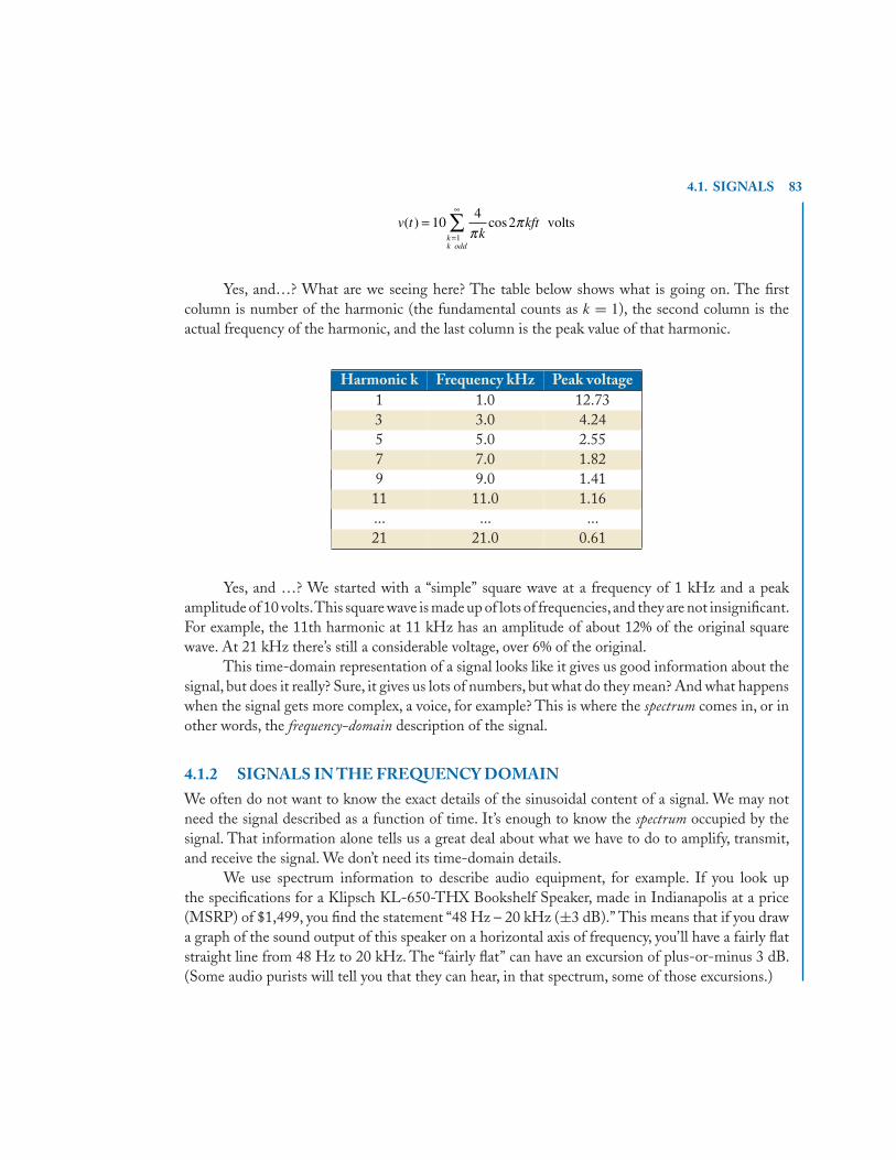
4.1. SIGNALS 83
v tk
kftkk odd
( ) cos==
∞
∑104
21 π
π volts
Yes, and…? What are we seeing here? The table below shows what is going on. The firstcolumn is number of the harmonic (the fundamental counts as k = 1), the second column is theactual frequency of the harmonic, and the last column is the peak value of that harmonic.
Harmonic k Frequency kHz Peak voltage1 1.0 12.733 3.0 4.245 5.0 2.557 7.0 1.829 9.0 1.4111 11.0 1.16... ... ...21 21.0 0.61
Yes, and …? We started with a “simple” square wave at a frequency of 1 kHz and a peakamplitude of 10 volts.This square wave is made up of lots of frequencies,and they are not insignificant.For example, the 11th harmonic at 11 kHz has an amplitude of about 12% of the original squarewave. At 21 kHz there’s still a considerable voltage, over 6% of the original.
This time-domain representation of a signal looks like it gives us good information about thesignal, but does it really? Sure, it gives us lots of numbers, but what do they mean? And what happenswhen the signal gets more complex, a voice, for example? This is where the spectrum comes in, or inother words, the frequency-domain description of the signal.
4.1.2 SIGNALS IN THE FREQUENCY DOMAINWe often do not want to know the exact details of the sinusoidal content of a signal. We may notneed the signal described as a function of time. It’s enough to know the spectrum occupied by thesignal. That information alone tells us a great deal about what we have to do to amplify, transmit,and receive the signal. We don’t need its time-domain details.
We use spectrum information to describe audio equipment, for example. If you look upthe specifications for a Klipsch KL-650-THX Bookshelf Speaker, made in Indianapolis at a price(MSRP) of $1,499, you find the statement “48 Hz – 20 kHz (±3 dB).” This means that if you drawa graph of the sound output of this speaker on a horizontal axis of frequency, you’ll have a fairly flatstraight line from 48 Hz to 20 kHz. The “fairly flat” can have an excursion of plus-or-minus 3 dB.(Some audio purists will tell you that they can hear, in that spectrum, some of those excursions.)

84 4. PROCESSING SIGNALS
Radio Shack describes their 5-Element Slimline LCR Speaker ($629.99) as “80 Hz – 21 kHz.”Any guess as to what that means? I have no idea how “flat” its curve is. (This is a plasma speaker;LCR means “left-center-right.”)
The diagram of Fig. 4.2 is the spectrum of the response of the normal human ear.The vertical
Figure 4.2: Sensitivity of human ear
unit is dB, but remember that dB requires a “zero” definition because it is always a ratio. Here,0 dB corresponds to a sound pressure of 2x10⁻⁵ pascals (I’m sure you wanted to know!). The dottedportions of the curve are the regions generally outside of normal hearing. Notice in the figure thatthe ear’s greatest sensitivity is around 3 kHz.
4.1.3 SIGNAL CONDITIONINGWhat might you want to do with a signal? The obvious choices are transmitting it and receiving it.But there are some other things we will want to do, though. One pretty clearly is to amplify it. Thesignal coming from the digital-to-analog converter in our CD player is very small but we want it todrive loudspeakers. We have to amplify that signal.
Another thing we often do to a signal is filter it. We want to change the spectrum of thesignal, altering the distribution of energy as a function of frequency. For example, the telephone hasa bandwidth of about 300 to 3,300 Hz for voice signals. If we are going to send an audio signalthrough the phone system, we will filter the signal to conform to the system’s allowed bandwidth.
4.1.4 EXAMPLE I—MAKING A SIGNAL SMALLERSuppose we want to control the level (amplitude) of a certain audio signal, a job we associate witha volume control or a fader in audio equipment. Figure 4.3 shows a device called a potentiometer, or

4.1. SIGNALS 85
Figure 4.3: Potentiometer or “pot”
more commonly, a pot. It’s set up as a voltage divider. The pot’s resistance is spread uniformly over330˚ of rotation. The slider rotates along that resistance to “pick off ” a fraction of the resistance.
The resistance of that fraction of the total of 10 k� is
Rθθ
=°
10330
k
That makes the output voltage
VR
V Vo s s= =°
θ θ10 330
This simple device makes the signal amplitude controllable from nothing to full value. Butvoltage dividers must not leak, meaning there must be no current leaving the divider junction. Sothis simple pot-based volume control can’t be connected to anything that requires current or theequation no longer applies.
Suppose this simple pot must be connected to an amplifier input that looks, to the pot, at least,like a 600-� resistor. This is a leaky voltage divider unless we isolate the divider from the amplifier’sinput. A voltage-follower op-amp circuit does this as in Fig. 4.4.
Figure 4.4: Pot with ouput isolated

86 4. PROCESSING SIGNALS
4.1.5 EXAMPLE II—AMPLIFIER WITH LIMITATIONSThe maximum output of a certain transducer is 0.8 mV. In other words, when this transducer isstressed/pushed/heated or whatever it is doing, the largest output voltage is just 0.8 mV.
This transducer feeds an instrumentation system that, for proper operation, requires an inputfrom 0 to ±0.5 V. This means we need an amplifier to take the small transducer signal and amplifyit for the instrumentation system. Because this system is dealing with fast-changing conditions, weare told that the bandwidth of the amplifier should be at least 10 kHz. We think, OK, this soundslike a job for an op-amp.
Op-amp? Why not? The op-amp circuit must have a gain of
V
Vinst
transducer
=×
=−
0 5
0 8 10625
3
.
.
Gee, that’s pretty large, but an inverting op-amp circuit could perhaps do this? Let’s see. Again of 625 would require 625 k� / 1 k�. That sounds suspicious because we have a general rulewith op-amps that resistors should be in the range of “a k-ohm to a few hundred k-ohms.” But625 k� isn’t too wild.
There is a worse problem hiding here, though—bandwidth. Amplifiers tend to have a responsethat “rolls off ” at higher frequencies. In other words, the higher the frequency, the smaller the gain.This characteristic is often expressed as the gain bandwidth product. It’s a number that says, the largerthe gain, the smaller the bandwidth.
The gain-bandwidth product for a common op-amp such as the TL072 is 3x10⁶ Hz. (Notethat gain is unitless and bandwidth is frequency.) For this gain-bandwidth product, the bandwidthfor a gain of 625 comes out
fbandwidth =×
=3 10
6254 8
6
. kHz
That’s way under 10 kHz that we require. So this amplifier arrangement doesn’t do the job.Let’s put two op-amps in cascade, each one providing part of the required gain. The gains of
amplifiers in cascade multiply if the amplifiers are truly independent. That means that connecting asecond amplifier’s input to the output of the first one doesn’t affect the output of the first one.
The required gain per stage is
Astage = =625 25
This circuit can be built with two identical stages, each with a 1-k� input resistor and a 25-k�
feedback resistor. The result is Fig. 4.5. The input of the second op-amp looks to the first one like1 k�, which is not a significant load for an op-amp’s output.

4.2. FILTERS 87
Figure 4.5: Cascade amplifiers
4.2 FILTERS
We’ve talked about signal conditioning already, or at least part of it. So far, we can make signalssmaller and larger, and we can adjust their amplitudes. There’s another major way that we conditionsignals—filtering. Signals often contain “parts” that we don’t want. An example is a signal thatcontains, in the form of interference, a significant amount of 60-Hz noise.
What’s the difference between noise and signal? Signal is the stuff we want and noise is thestuff we don’t want. What’s one person’s signal is another person’s noise. If you are listening to yourfavorite music in one room and your friend is listening to different music in another room, to eachof you, your music is your signal. But if your friend’s music is too loud and you are hearing it, that’snoise to you.
How do you eliminate that noise? How do you eliminate your friend’s music to keep it frominterfering with yours? Close the door! But does that eliminate the noise? Or just reduce it to whereit doesn’t bother you? Probably the second. That’s filtering.
We are going to keep our study of filters fairly simple. Our filters will all be one-pole filters.Thatmeans that all our filters denominators that have a single term of the form (1 + s/a). Rememberingthat if we replace s = jω, this term becomes (1 + jω/a). We’ll see how to use this shortly.
4.2.1 BASIC FILTER FORMSThere are four basic forms of one-pole filters:
Low-pass (LP): This filter passes low frequencies and attenuates high frequencies. ExampleIII (Chapter 1, Section 1.2.3) is a low-pass filter with a break frequency of 2,000 radians persecond and a pass-band gain of 6 dB.
High-pass (HP): This filter passes high frequencies and attenuates low ones. Example IV(Chapter 1, Section 1.2.4) is a high-pass filter. Its break frequency is 500 radians per second;its pass-band is gain is 14 dB.

88 4. PROCESSING SIGNALS
Band-pass (BP): This filter passes only a portion of the frequencies in the signal. Example V(Chapter 1, Section 1.2.5) is a band-pass filter. Its pass band is between 150 and 2,500 radiansper second. In its pass band, the gain is 27 dB. This is a two-pole filter, but we’ll design oursin this chapter using a high-pass filter and a low-pass filter in cascade.
Band-stop or notch: This filter stops or cuts out a portion of the frequency spectrum. A goodnotch filter is more complicated because it generally needs multiple poles. We are not goingto deal with one in this chapter.
4.2.2 BREAK FREQUENCY AND HALF-POWERThe relationship between the break frequency, the pole, and the actual filter performance is animportant one. Consider a filter whose voltage transfer function is
H sV
V
ks
a
out
in
( ) = =+1
Replace s by jω:
H sV
V
kj
a
out
in
( ) = =+1
ω
We evaluate this at ω = a, which we should remember from Bode diagrams as the breakfrequency:
H sV
V
kja
a
k
jout
in
( ) = =+
=+1 1 1
The magnitude of this result is important:
H s jak
j
kk( ) .= =
+= =
1 1 20 707
In dB, the magnitude of H at this break frequency is
H s jak
k
k dB
dB
dB
( ) log log log= = = −
= −
202
20 20 2
3
This says the actual magnitude of the filter’s response is 3 dB inside the Bode asymptotes atthe break frequency.

4.2. FILTERS 89
The magnitude at the break frequency is k/√
2. Since the transfer function H(s) is a voltageratio, this
√2 says that the voltage is smaller by a factor
√2. Because power is proportional to voltage
squared, the power passing through the filter at this break frequency must be smaller by a factor(√
2)2 = 2. In other words, the power is half as large as in the passband. This leads us to call thebreak frequency the half-power point.
In our original H(s), the frequency s = jω = ja is important:
• ω = a is the break frequency where the Bode asymptotes meet.
• At ω = a, the denominator of H(s) is 1 + j1.
• If the denominator is 1 + j1, the magnitude of the denominator is√
2.
• This√
2 is 3 dB, so the actual response curve is 3 dB inside the Bode asymptotes.
•√
2 is in the denominator, so the power (√
2)2 = 2 is half as much, which is why we call thebreak frequency the half-power point.
This will all hang together better with some examples.
4.2.3 EXAMPLE III—LOW-PASS PASSIVE FILTERThe circuit of Fig. 4.6 is a single-pole, passive, low-pass filter. We are going to be interested in the
Figure 4.6: Low-pass passive filter
filter’s transfer function H(s) = Vo/Vs and how those characteristics come about:
• There is going to be just one pole (a root of the denominator) in H(s) because there is just oneenergy-storage element, the capacitor. This will yield just one term in s
• A passive filter, or more generally, a passive circuit is one with no amplifier, no active element.It’s constructed with just R, L, and C elements. As we’ll see soon, though, we generally aregoing to want an amplifier somewhere in the circuit.
• How can we know that it is low-pass? Look at where the capacitor is in the circuit.Then recallthat the impedance of a capacitor, 1/sC, decreases in magnitude as the frequency increases. At

90 4. PROCESSING SIGNALS
d-c, the capacitor looks like an open circuit and has no effect on the voltage. As the frequencyincreases, the capacitor’s impedance decreases, which in effect begins to “short out” the outputterminals. Hence, as frequency increases, output decreases.
It’s probably easiest to find the transfer function H(s) and then the Bode diagram by usingthe voltage-divider relationship. The impedance of the capacitor is
ZsC =
× −
1
0 01 10 6.
Now write the voltage divider for H(s):
H sV
V
Z
R Z
s
s
o
s
C
C
( )
.
.
= =+
= ×
+×
=−
−
10 01 10
20001
0 01 10
1
1
6
6++ × −20 10 6 s
This needs to be in the standard form for making Bode diagrams as we did in Section 1.2.All terms involving s need to be written as 1 + s/a:
H sV
V so
s
( ) = =+
×
1
150 103
The Bode diagram has two asymptotes:
• The numerator is 1, which in dB is 20 log 1 = 0 dB, so this asymptote is a horizontal line at0 dB.
• The denominator has a break frequency of 50x103 radians/second. To the left of that break,the curve is a horizontal line at 0 dB; to the right, the curve slopes downward at 20 dB/decade.
These asymptotes are logarithms (dB), so we combine them by addition. The result is theBode diagram of Fig. 4.7. It’s flat at 0 dB up to ω = 50 krad/s. Then it slopes downward at 20 dBper decade. This diagram also includes the smooth line of the actual curve as well as the asymptotes.Notice that the smooth curve is 3 dB “inside” the asymptotes at the break frequency. (It’s inside by1 dB at half and twice the break frequency.) This half-power point or 3 dB point comes from
H s jj j
H j
= ×( ) =+ ×
×
=+
=
×(
50 101
150 1050 10
1
1 1
1
2
50 10
33
3
3 )) = = −dB
201
23log dB

4.2. FILTERS 91
Figure 4.7: Bode plot for Example III
There! A passive low-pass filter! Now what are we going to do with it? I presume we had areason for filtering the particular signal Vs , so we must have something in mind that we are planningto pass the signal to. But what?
Umm, OK, how about feeding another circuit, maybe a controller? Sure, but let’s be careful.We analyzed the filter by using the voltage-divider relationship, which requires that the divider not“leak.” There can be no current flowing to the right from the R-C node. So what circuit can weconnect to?
How about the voltage follower in Fig. 4.8? The op-amp’s input circuit draws essentially no
Figure 4.8: “Improved” low-pass filter
current, so it won’t mess up the voltage divider. Philosophically, this seems to violate the passive idea.Well, while we are at it, how about putting in an op-amp circuit with gain? This way, we not
only filter the signal but we amplify it. OK, sounds good. Let’s add a gain of 2 to see what happens.I’ll add an inverter with a 1-k� input resistor and a 2-k� feedback resistor as shown in Fig. 4.9.
NO! NO! That won’t do! The input to the inverter draws current through the 1-k� resistor.This has altered the voltage divider. The inverter won’t work.
The non-inverter will do the job as shown in Fig. 4.10. Its input terminal draws almost nocurrent, so it doesn’t affect the divider. So now we have an active low-pass filter with a pass-bandgain of 2 and a cutoff frequency of 50x103 radians per second.

92 4. PROCESSING SIGNALS
Figure 4.9: INCORRECT low-pass filter
Figure 4.10: Better low-pass filter
There’s a better way to do this, as the next example shows.
4.2.4 EXAMPLE IV—ACTIVE LOW-PASS FILTERThis time I want an active low-pass filter. Its break frequency is to be 50x103 radians/second. Itspass-band gain is to be 2. This can be done using the inverter of Fig. 4.11. Here’s how it works:
• The R and the C in the feedback path provide the filter aspect of the circuit. These are thesame values as in the previous example and provide the same break frequency.
• At very low frequencies such as d-c, the capacitor is not a factor, so this inverter has a low-frequency gain of −2 via the two resistor values.
Analysis of this circuit is most easily done by first finding the impedance of the feedback pathand then using our knowledge of the inverter to get H(s).
The impedance of the feedback path is

4.2. FILTERS 93
Figure 4.11: Even better active low-pass filter
Zs s
s
f = ×=
× +
=+
×
−−
1
0 01 102000
1
0 01 101
20002000
150
66. .
1103
Using what we know about the inverter:
H sV
V
Zs
o
s
f( ) = = − =−
+×
1000
2
150 103
The Bode diagram (Fig. 4.12) has an asymptote for the “2” at 6 dB and a break downward at50x103 radians/second.
4.2.5 RC AND BREAK FREQUENCYNotice how the product RC keeps appearing in the equations for these filters. In general, an R thatcan be “seen” by a C sets the break frequency. That frequency will be
ω
ωπ π
break
breakbreak
RC
fRC
=
= =
1
2
1
2
What does “seen” mean? If an R and a C are in parallel, C sees that R. If they are in series,likewise, C sees that R. So we can generally determine the break frequency of one-pole filters bylooking at the capacitor and noting what resistance it sees.

94 4. PROCESSING SIGNALS
Figure 4.12: Bode plot for Example IV
4.3 MORE EXAMPLEIn the examples that follow, we’ll design active filters to meet frequency and gain specifications. I’mnot going to attempt to use standard values of resistors and capacitors. If these filters are to be built,the element values will probably need to be altered to fit what is available. Resistor values presentlittle problem because the 1%-series of resistances can handle all but the most demanding precisionfor a filter. Capacitors are harder to find with precise values.
4.3.1 EXAMPLE V—LOW-PASS ACTIVE FILTERDesign a low-pass filter with the following specifications:
• Cutoff (break) frequency of 4 kHz
• Pass-band (low-frequency) gain of 8 dB
• Input resistance at least 1 k�
I’ll start by choosing the input resistor to be 1 k�.This is simple and meets the third specifica-tion.That choice leads to the choice of the feedback resistor, which will determine the low-frequencygain.
The low-frequency or pass-band gain is given in dB, so it needs to be changed to a plainnumber A:
8 20 logdB A=
Turning this around to find A:
8
2010 10
10 2 5
8 20
8 20
=
= =
= =
log
.
log
A
A
A
A

4.3. MORE EXAMPLE 95
So if the input resistor is 1 k�, the feedback resistor needs to be 2.5 k� to provide a gain of2.5. (Actually, the gain is –2, but we’ll ignore the inversion.)
The break frequency or the cutoff frequency (two names for the same thing) is determined by1/RC in radians/second, where R and C are in parallel in the feedback path. R is already set to be2.5 k�, so we need to find C, not forgetting to translate via 2π from hertz to radians/second:
12 4 10 2 5 10
1
2 5 10 2
3 3
3
R CR
C
f ff
f
= ( ) ×( ) = ×
=×( )( )
, .
. 44 101 59 10
0 016
3
8
×( )= ×.
. F
This filter is in Fig. 4.13 and its Bode diagram is Fig. 4.14.
Figure 4.13: Low-pass filter—Example V Figure 4.14: Bode plot for Example V
4.3.2 EXAMPLE VI—HIGH-PASS ACTIVE FILTERDesign a high-pass filter as follows:
• Cutoff frequency of 800 Hz
• Pass-band (high-frequency) gain of 1
This time the input resistance is not specified, so I’ll just pick one—how about 1 k�? Thatmeans…whoa! Wait a minute. What is the circuit for a high-pass filter? The filter with a parallelRC in the feedback path is low, not high.
Suppose I put a capacitor in series in the input path as shown in Fig. 4.15. Now find H(s) forthis circuit. The input impedance is
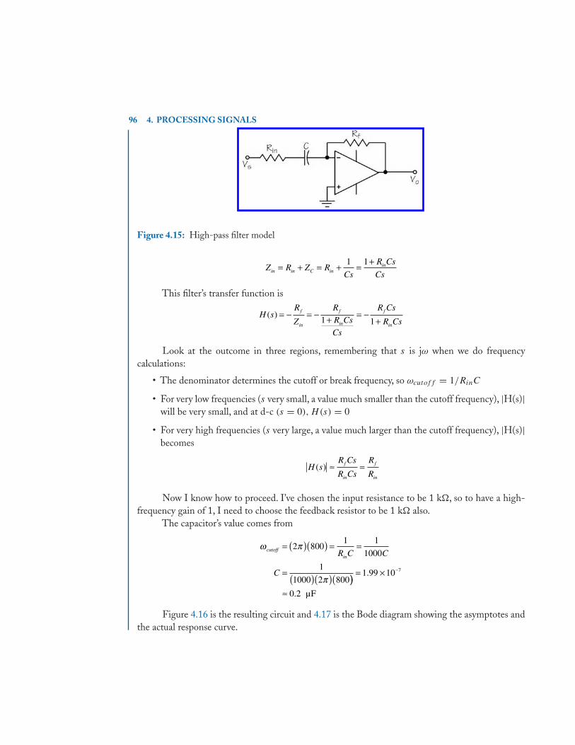
96 4. PROCESSING SIGNALS
Figure 4.15: High-pass filter model
Z R Z RCs
R Cs
Csin in C inin= + = + =
+1 1
This filter’s transfer function is
H sR
Z
RR Cs
Cs
R Cs
R Csf
in
f
in
f
in
( ) = − = − + = −+1 1
Look at the outcome in three regions, remembering that s is jω when we do frequencycalculations:
• The denominator determines the cutoff or break frequency, so ωcutoff = 1/RinC
• For very low frequencies (s very small, a value much smaller than the cutoff frequency), |H(s)|will be very small, and at d-c (s = 0), H(s) = 0
• For very high frequencies (s very large, a value much larger than the cutoff frequency), |H(s)|becomes
H sR Cs
R Cs
R
Rf
in
f
in
( ) ≈ =
Now I know how to proceed. I’ve chosen the input resistance to be 1 k�, so to have a high-frequency gain of 1, I need to choose the feedback resistor to be 1 k� also.
The capacitor’s value comes from
ω π
π
cutoffinR C C
C
= ( )( ) = =
= ( )( )(
2 8001 1
1000
1
1000 2 800)) = ×
≈
−1 99 10
0 2
7.
. μF
Figure 4.16 is the resulting circuit and 4.17 is the Bode diagram showing the asymptotes andthe actual response curve.

4.3. MORE EXAMPLE 97
Figure 4.16: High-pass filter—Example VI
Figure 4.17: Bode plot for Example VI
4.3.3 EXAMPLE VII—BAND-PASS ACTIVE FILTERDesign a band-pass filter for voice in telephone circuits:
• Lower cutoff at 300 Hz
• Upper cutoff at 3.3 kHz
• Pass-band gain of 10 dB
I think a good way to start this one is to look at the Bode diagram that meets these specifica-tions. See Fig. 4.18 and notice the following:
• There are two break frequencies, 300 and 3300 Hz
• Below 300 Hz, the slope is 20 dB/decade
• Above 3300 Hz, the slope is −20 dB/decade
• In the middle between the cutoff frequencies, the gain is 10 dB
A simple way to do this job is to consider this filter to be the combination of two that wealready know about, a low-pass filter and a high-pass filter. Perhaps surprisingly, we can do this withjust one op-amp as Fig. 4.19 shows.The series RC on the input provides the high-pass characteristic,while the parallel RC in the feedback path provides low-pass.
We need to be careful not to think backward, though! The high-pass characteristic providesthe 300-Hz break, while the low-pass characteristic provides the 3300-Hz one. It’s easy to mix highand low here. These will yield two equations:
ω
ω
lowerin in
upperf f
R C
R C
=
=
1
1

98 4. PROCESSING SIGNALS
Figure 4.18: Specifications for Example VII
Figure 4.19: Band-pass filter model
(Be careful of radians and hertz!)But this is just two equations and there are four elements. Now what? Well, consider the pass
band between the cutoffs. That part of the curve is the pass band of both the high-pass and thelow-pass filters. If we think back to those simple filters, in the pass bands their resistors dominated.In the pass band of both high-pass and low-pass filters, the input and feedback resistors set the gain.
The same is true here as long as the cutoff frequencies aren’t too close together. A decade isabout enough for “not too close.” In this region, the gain of the band-pass filter is approximately–Rf /Rin. That gives me another equation, where the “10” in the exponent is my desired pass-bandgain of 10 dB:

4.3. MORE EXAMPLE 99
R
Rf
in
= =10 3 1610 20/ .
That’s now three equations and four unknowns. What about the fourth equation? We don’thave one, so we simply have to choose a value for one of the elements and go from there.
But which one? It turns out that capacitors are often the best elements to “just pick.” I will pickthe capacitor that is likely to be the largest one in the circuit. If I look at the two cutoff equations, Inote that the lower frequency, the larger the capacitor. So I am going to choose
Cin = 0 1. μF
This value for C is about as large as practical for small-sized commercial capacitors.That gives me the value for Rin:
RCin
lower in
= =( )( ) ×( )
=1 1
2 300 0 1 105 31
6.. k
I can now calculate Rf :
R
R
R
f
in
f
=
= ( ) ×( ) =
3 16
3 16 5 31 10 16 83
.
. . . k
Finally, I get Cf :
CRf
upper f
= = ( )( ) ×( )= × =−
1 1
2 3300 16 8 10
2 88 10 0
3
9
ω π .
. .000288 μF
That does it and the result is the circuit of Fig. 4.20.But does this circuit do the job? I’m going to finish all this by calculating the frequency
response of this circuit using the actual element values and checking at least three points, namely,the values of the transfer function at the two break frequencies and at the middle of the pass band.
This calculation is most easily done by finding the impedances of the input and feedbackpaths first:
Zs s
Z
f
in
=×
× =×
+ ×
=
− −
1
2 88 1016 8 10
16 8 10
1 4 84 1093
3
5..
.
.
55 31 101
0 1 10
1 5 31 10
0 1 103
6
4
6.
.
.
.× +
×=
+ ××−
−
−s
s
s

100 4. PROCESSING SIGNALS
Figure 4.20: Band-pass filter—Example VII
Their ratio yields the overall transfer function:
H sZ
Zss
f
in
( )
...
.
= − = −
×+ ×+ ×
−
−
16 8 101 4 84 101 5 31 10
0
3
5
4
11 101 68 10
1 4 84 10 1 5 31 10
6
3
5 4
×
= −×
+ ×( ) + ×(
−
−
− −
s
s
s s
.
. . ))From the poles in the denominator, the two break frequencies turn out to be
f
f
lowerlower
uppe
= = ×( ) =− −ωπ π2
1
25 31 10 299 74 1. . Hz
rrupper= = ×( ) =− −ωπ π2
1
24 84 10 3 2885 1
. . kHz
How about the gain at the middle of the pass band? I’ll chose the middle by eye to be about1 kHz. The magnitude of the transfer function at this frequency is
H jj
j j( )
.
. .ω ω
ω ω=
×+ ×( ) + ×( )
−
− −
1 68 10
1 4 84 10 1 5 31 10
3
5 4
AAt dBω π ω= ( )( ) = =2 1000 2 900 9 25, ( . .H j
Figure 4.21 is the Bode diagram with the actual curve drawn on the desired asymptotes. Youcan judge whether this design does the job!
4.4 SUMMARYWe’ve processed a few signals, mostly by filtering, all by analog devices. We’ve done this filteringby using just two very straightforward one-pole filters, low-pass and high-pass. Each involves just

4.4. SUMMARY 101
Figure 4.21: Actual plot for Example VII
one capacitor and one resistor, but each is made more versatile by adding one op-amp to make it anactive filter. More extensive filters can be built up from these simple ones.


FORMULAS AND EQUATIONS 103
FORMULAS AND EQUATIONS1. Break frequency for single R-C pair (either series or parallel)
ω
ωπ π
break
breakbreak
RC
fRC
=
= =
1
2
1
2
2. Low-pass active filter
3. High-pass active filter
4. Band-pass active filter


105
C H A P T E R 5
Electromagnetic CompatibilityHuh? What’s this electro…something-or-other? Well, how about noise noise NOISE? Callingthis electromagnetic compatibility is just a way of stating the positive side of the problem rather thanthe negative. Instead of screaming at the kids to stop hammering on the coffee table, you arrangefor something else they can bang on.
We live in a noisy world, not just audible noise but electrical noise as well. This electricalnoise can interfere with the proper operation of electrical apparatus such as instruments, controlsystems, communications links, and computers. Compatibility implies that we design our systemsso that electrical noise does not disturb them unduly—and our systems don’t disturb others unduly,either.
Have you ever read the required statement on RF Emissions that comes with just about everypiece of electronics today? It says in part, “Operation is subject to the following two conditions: (1)This device may not cause harmful interference, and (2) This device must accept any interferencereceived, including interference that may cause undesired operation.”
This says that we have to consider how to protect our systems from electrical interference sothat they continue to operate properly in the face of that interference. In other words, let the kidskeep banging on the coffee table, ignore the din, and go about your work.
In this chapter we look at the kinds of interference that our systems must put up with, howthat interference is coupled into our systems, and how we might keep it out or at least diminish itseffects.
5.1 NOISE
Noise is pretty easy to define. It’s the same as signal but it’s signal we don’t want. What’s oneperson’s signal is another person’s noise. Electromagnetic noise is unwanted energy that is conveyedelectrically or magnetically into your system. It is a problem if it interferes with the proper operationof that system. Our job is to design our systems so that noise doesn’t bother their functioning.
Figure 5.1 looks at a system as being a source of information, a channel over which theinformation is transmitted, and a destination that uses that information. This doesn’t have to bea communications link like a telephone wire or a radio signal. It can be a memory chip that iscommunicating with a processor on the same circuit board.
Electrical noise can enter this system everywhere as the diagram shows.Noise is always present,so it’s our job either to keep it out or to reduce its effect on our system. But we cannot keep it out100%. Hence, we need to learn about how this noise gets in before we can figure out how to stop it.

106 5. ELECTROMAGNETIC COMPATIBILITY
Figure 5.1: Interference
There are two general categories of electrical noise, and we deal with them in somewhatdifferent ways:
Pulse noise: This noise, generally called an electromagnetic pulse (EMP) is sometimes mentionedin the media as the outcome of a nuclear explosion. But we see EMP quite often in the formof lightning. A lightning strike nearby produces a large pulse of energy that can couple intoour systems and destroy components. This can happen even if the strike is merely nearby, notdirect.
There are other common sources of pulse noise. Direct-current motors are a prime source,where the brushes switching from one commutator segment to another cause noise. Power-line switching transients and switching power supplies (in every computer) are also sources.
Continuous noise: An obvious source is a nearby radio transmitter, some of whose energy couplesinto our system. Any piece of 60-Hz equipment is a source of possible 60-Hz noise, even thelights in the room.
Noise gets into our systems through three mechanisms:
• Capacitive coupling is simply a capacitance that is formed between two conductors. Since acapacitor is just two metal plates separated by a dielectric, two wires near one another can bea capacitor. There’s nothing that says the metals have to be flat plates.
• Magnetic coupling comes about because a current in a wire or coil of wire creates a magneticfield that can couple into another conductor.
• Electromagnetic radiation enters “over the air” in the same way broadcast signals come fromradio stations.
Our job is to understand a bit about these three mechanisms. Our goal, of course, is to keepthe energy out, but that’s not 100% possible, so we will seek ways to diminish the unwanted effects.
5.2 CAPACITIVE COUPLINGSince capacitive coupling implies the existence of capacitance, we can model this form of interferenceby a simple circuit with a capacitor “connection.” There are two circuits in Fig. 5.2. The one on the

5.2. CAPACITIVE COUPLING 107
left is the source of the noise and is modeled as just a voltage source.The one on the right, often calledthe victim circuit, is receiving the noise. The capacitor over the top represents capacitive coupling.
Figure 5.2: Capacitive coupling
5.2.1 CALCULATING CAPACITIVE COUPLINGIn order to understand the effects of this coupling, we need to see how much of the noise voltagemakes its way into the victim circuit. If we assume that both of these circuits are linear, we can applythe principle of superposition. This principle says that we can look at the effects of just one sourceat a time while insuring that the other sources are dead.
If we apply superposition to the circuit of Fig. 5.2, we leave the noise-voltage source VN
turned on and we turn off the signal source VS . “Turning off ” means we replace the source with ashort circuit to guarantee that the voltage where it was is zero. The result is the circuit of Fig. 5.3.
Figure 5.3: Victim with VS = O
The two resistors of the victim circuit are in parallel, so I’ll reduce the circuit to the onlyelements affected by the noise voltage (Fig. 5.4): the source of the noise VN , the coupling capacitorCC , and the resistors of the victim circuit, labeled RO . (RO is RS in parallel with RL.)
The circuit is a voltage divider, so I can figure out the voltage VL coupled into the victim:

108 5. ELECTROMAGNETIC COMPATIBILITY
Figure 5.4: Noise coupling only
V VR
Rj C
R R RL NO
OC
O S L=+
=1
ω
where
This twists around to become
V V
j C R
L N
C O
=+
1
11
ω
The magnitude of the coupling is what we want to look at:
V
V
C R
L
N
C O
=+
1
11
2 2 2ω
Consider what happens at the ends of the frequency range:
V
VL
N
==→ ∞
⎧⎨⎩
⎫⎬⎭
0 0
1
ωω
OK, are you ready for an obvious statement? Coupling gets worse as the frequency goes up.So if that’s the case, what do we do to reduce this interference? It’s not hard to figure out what toattack:
• The operating frequency of our circuit is fixed by the requirements of whatever we are doing.So the frequency ω is fixed.
• The impedance of our victim circuit (here, RO) is fixed by the needs to our circuit. We perhapscould lower the impedance because making it smaller makes the denominator of |VL / VN |larger and reduces the coupling. But we might not have that choice because of the design ofour circuit.

5.2. CAPACITIVE COUPLING 109
• That leaves just the coupling capacitance CC to adjust. Reducing the coupling capacitancemakes the denominator of |VL / VN | larger and reduces the voltage coupled into our victimcircuit.
Sure, this outcome should have been obvious! If you want to reduce the capacitive coupling,reduce the coupling capacitance! By going through the calculations, though, we did see what optionsmight have been available to us.
5.2.2 REDUCING CAPACITIVE COUPLINGRather than looking at the capacitance between two wires, which is a messy equation, let’s look atthe simpler case of a parallel-plate capacitor:
CA
d=ε
This says that capacitance is proportional to the area of the plates. Since the “plates” in ourinterference problem are really wires that have been chosen for being the proper ones for whateverwe are doing, we can’t change those.
The equation also says that capacitance is inversely proportional to the distance between theplates. That’s our clue as to how to reduce capacitive coupling—separate the conductors further.(OK, if you were really expecting something more complicated, sorry!)
But surprisingly, there is another way: add capacitance to the circuit. Yes, add! But add thiscapacitance in a special way. We do this by adding a conducting ground plane near the wires thatare interfering with one another.
The drawing of Fig. 5.5 shows two wires end on. Between the two wires is the coupling
Figure 5.5: Conductors over ground
capacitance CC . From each of the wires to the ground plane is the ground capacitance CG. Eventhough this seems strange, it works. In an overly simple way, the ground plane “diverts” some of theelectric field away from coupling the two conductors.
I’ll add the noise voltage source VN and the victim’s resistance RO to the drawing (see Fig. 5.6).Then I can analyze the circuit as before. The voltage divider consists of RO in parallel with CG asone leg and the coupling capacitance CC as the other:

110 5. ELECTROMAGNETIC COMPATIBILITY
Figure 5.6: Conductors over ground in circuit
V V
j C Z
where Z Rj CL N
C O
O OG
=+
=1
11
1
ωω
The noise coupling will be reduced, meaning that will be smaller if
j C Z j C R
Z R
C O C O
O O
ω ω<
<
Adding CG in parallel with RO does yield an impedance whose magnitude is smaller thanRO , so it looks like this will work. Let’s try some numbers.
5.2.3 EXAMPLE I–BENEFIT OF GROUND PLANETwo conductors are spaced 3 mm apart (Fig. 5.7). There is no ground plane nearby. The circuits
Figure 5.7: Parallel conductors coupling
have been simplified to just the noise source, the coupling capacitor, and the resistances of the victimcircuit.
The wires are #22 American Wire Gauge (AWG), whose diameter is 0.644 mm. Both wiresare one meter long. Capacitance per meter of two wires in parallel is
Cd rC = ( )
27 78.
lnpF/m

5.2. CAPACITIVE COUPLING 111
where d is the spacing of the wires and r is the radius of the wire. Using this formula, the couplingcapacitance is
CC = ( ) =27 78
3 0 32212 4
.
ln .. pF/m
The noise source is operating at 100 MHz (in the middle of the FM broadcast band). Bothresistances RS and RL are 75 ohms, so RO = 37.5�. From the voltage divider that we developed inSection 5.2.1, the noise voltage coupled into the victim circuit is
V
Vj C R j
L
N
C O
=+
=+ ( )( ) ×( )(−
1
11
1
11
2 10 12 4 10 37 58 12ω π . . ))= ∠ °0 280 73 7. .
Now let’s see what adding the ground plane does to this. The circuit of Fig. 5.8 shows thecircuit with the capacitances to the ground plane. The conductors are each 0.2 mm from the groundplane.
Figure 5.8: Conductors with ground plane
The formula for capacitance per meter of a wire over a ground plane is
Ch rC = ( )
27 78
2
.
lnpF/m
where h is the height of the wire above the plane and r is the radius of the wire. This formula givesa ground capacitance of
CC = ( )( ) =27 78
2 0 2 0 322128 1
.
ln . .. pF/m
In the circuit of Fig. 5.8, the capacitor on the left has no effect because the voltage source isdirectly across it.The voltage divider is a resistor and capacitor for one leg and the coupling capacitorfor the other. The impedance of the vertical leg is

112 5. ELECTROMAGNETIC COMPATIBILITY
Zj
O =+ ( )( ) ×( )
= ∠ − °
−
11
37 52 10 128 1 10
11 8 71 7
8 12
..
. .
π
The noise voltage coupled into the victim circuit is now
V
Vj
L
N
=+ ( )( ) ×( ) ∠ − °( )
=
−
1
11
2 10 12 4 10 11 8 71 7
0
8 12π . . .
.00845 16 8∠ °.
Did this do any good? The added capacitance to the ground plane drops the coupling from0.280 to 0.0845. That’s 10.4 dB. That’s one reason why circuit boards for high-speed logic (likecomputers) usually include a ground plane between layers of circuit traces.
5.3 MAGNETIC COUPLINGMagnetic coupling is another mode by which energy sneaks from one circuit to another, bringingwith it unwanted energy that we call noise.
Figure 5.9 shows a conductor carrying a current, along with the resultant magnetic flux densityB. The magnitude of this flux density is
Figure 5.9: Field around conductor
B HI
r= =μ μ
π2
Coupling a voltage into another circuit depends on the total flux:
Vd
dt
d BA
dtN = = ( )ψ
If the area A is constant, this becomes
V AdB
dtN =

5.3. MAGNETIC COUPLING 113
Since the only thing changing is the current, the coupled noise voltage is
VA
r
dI
dtN =μπ2
Now suppose the current is sinusoidal:
I I to= cosω
Then the noise voltage is
V I tA
rN o= −( )⎛⎝⎜⎞⎠⎟
ω ω μπ
sin2
whose peak magnitude is
VA
rI B AN o= =
μπ
ω ω2
How do we reduce this voltage? We could change the frequency ω but that’s generally fixedby the signal requirements, so we are left with three other choices:
• Reduce the area of the victim circuit that is being presented to the magnetic flux
• Increase the distance between the noise source and the victim circuit, thereby reducing B
• Change the angular relationship between the two circuits, since magnetic coupling dependsvery much on this relationship (although we have left it out of the analysis)
The third method is one that isn’t hard to do. Consider the cable of Fig. 5.10. The output
Figure 5.10: Parallel conductors: 1 loop
voltage Vo will be the sum of the two voltage sources, signal and noise:
V V VO S N= +
Now twist the wires so there are three loops (Fig. 5.11):Two of the loops cancel each other, so let’s keep going—how about six twists (Fig. 5.12)?

114 5. ELECTROMAGNETIC COMPATIBILITY
Figure 5.11: Parallel conductors: 3 loops
Figure 5.12: Parallel conductors: 6 loops
V V V V VO S N N N= + − +3 3 3
This sounds too good to be true, and it probably is.The common practice is to use a reductionby the number of twists:
V V VO S N= + 6
Convention is that n should be limited to 1,000 twists; going beyond that yields unrealisticnumbers.
Figure 5.13 is a communications cable. This one is a Belden cable with two twisted pairs
Figure 5.13: Communications cable

5.4. ELECTROMAGNETIC SHIELDING 115
separated in foil shields. The conductors are #22 AWG. They are color-coded so that they canbe easily identified. Notice especially the aluminized Mylar shields that surround the pairs. Theseprovide ground planes and the separation between the pairs. The thin bare wire is a drain thatprovides a solid ground conductor through the cable.
Figure 5.14 is an Ethernet cable. This one is a Cat 5 cable. It has no shields, but it makes
Figure 5.14: CAT 5 cable
clever use of twists. Each of the four pairs is twisted, but the twists are different. The numbers oftwists per inch are not integral multiples of one another so the twists of one don’t stay in step withthe twists of the others.
5.4 ELECTROMAGNETIC SHIELDING
The third mode by which energy enters our circuits is electromagnetic radiation. While that soundsdangerous, this is the non-ionizing radiation that is produced intentionally by every radio transmitterand unintentionally by just about every other electronic device. In the right places, this energy isbeneficial, bringing information and music or cooking our food in the microwave oven. In our circuits,though, it is just noise.
We’ve considered how one circuit can affect another by both capacitive and inductive coupling.We’ve seen how one might separate circuits by adding ground planes or by changing orientation.Now we need to look at how we can keep this radiated energy out of our circuits. The answer isshielding.
A good example of the need for shielding is your computer.All computers generate a significantamount of electrical noise because of all the high-speed pulses in their circuits. Much of the shieldingof computers is to keep their noise inside, not letting it out to affect other circuits and electronics.The Federal Communications Commission has very strict rules on how much electrical noise canbe allowed to escape from electronic devices such as computers.
What does shielding mean? It means constructing a barrier between the noise source and therest of the world. Figure 5.15 shows two circuits separated by a shield. Circuit 1 is radiating electricalenergy. The shield is to keep that energy out of Circuit 2. Keep in mind that this energy is arrivingnot from capacitive effects and not from magnetic effects but directly by electromagnetic radiation.
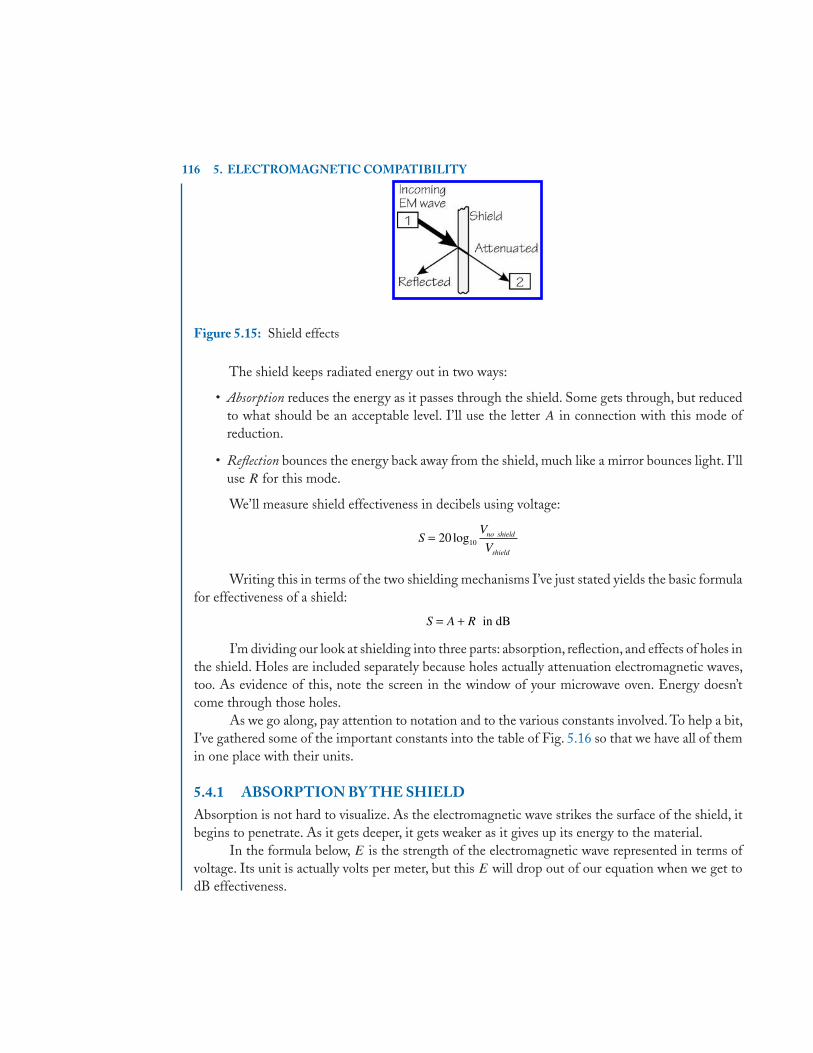
116 5. ELECTROMAGNETIC COMPATIBILITY
Figure 5.15: Shield effects
The shield keeps radiated energy out in two ways:
• Absorption reduces the energy as it passes through the shield. Some gets through, but reducedto what should be an acceptable level. I’ll use the letter A in connection with this mode ofreduction.
• Reflection bounces the energy back away from the shield, much like a mirror bounces light. I’lluse R for this mode.
We’ll measure shield effectiveness in decibels using voltage:
SV
Vno shield
shield
= 20 10log
Writing this in terms of the two shielding mechanisms I’ve just stated yields the basic formulafor effectiveness of a shield:
S A R= + in dB
I’m dividing our look at shielding into three parts: absorption, reflection, and effects of holes inthe shield. Holes are included separately because holes actually attenuation electromagnetic waves,too. As evidence of this, note the screen in the window of your microwave oven. Energy doesn’tcome through those holes.
As we go along, pay attention to notation and to the various constants involved. To help a bit,I’ve gathered some of the important constants into the table of Fig. 5.16 so that we have all of themin one place with their units.
5.4.1 ABSORPTION BY THE SHIELDAbsorption is not hard to visualize. As the electromagnetic wave strikes the surface of the shield, itbegins to penetrate. As it gets deeper, it gets weaker as it gives up its energy to the material.
In the formula below, E is the strength of the electromagnetic wave represented in terms ofvoltage. Its unit is actually volts per meter, but this E will drop out of our equation when we get todB effectiveness.

5.4. ELECTROMAGNETIC SHIELDING 117
Figure 5.16: Table of useful constants
E E eox= − δ
In this equation, Eo is the field strength at the surface of the shield material, x is the distanceinto the shield, and δ is a physical property called the attenuation constant or the skin depth.
Convert this to dB to get the effectiveness by absorption:
AE
E e
teo
ot
=⎛⎝⎜
⎞⎠⎟=−20 2010 10log logδ δ
The result is a very simple formula for absorption effectiveness, where t is the thickness of theshield:
At
= 8 69.δ
in dB
The skin depth δ depends on the frequency ω in radians per second, the permeability of thematerial μ, and the conductivity of the material σ :
δωμσ
=2
Skin depth can also tell us something about choosing conductors, which sounds a bit strange.Let’s calculate the skin depth at 60 Hz:
δπ π
= ( )( ) ×( ) ×( )=
−
2
2 60 4 10 5 96 10
8 4
7 7.
. mm
This says that the electromagnetic field is only one-third (actually, 1/e) as strong about onecentimeter into the copper conductor, so the middle of the conductor carries less current than theoutside does.The message: It isn’t economical to use very large conductors—several smaller ones areless wasteful of copper.

118 5. ELECTROMAGNETIC COMPATIBILITY
5.4.2 REFLECTION BY THE SHIELDReflection of electromagnetic energy is not intuitive, although we are certainly familiar with mirrors.Energy reflected from a shield surface reflects in much the same way as light does from the mirror.
Light reflection depends on the difference between the indices of refraction of the air and theglass (or whatever materials we are dealing with). Electromagnetic energy reflection depends on thedifference between the impedances of air and the shield. So we need these impedances.
The impedance of free space (and hence of air) is
Z00
0
377= =
The impedance of the shield material is
Zm =
where μ will be μo unless the shield is made of an iron-bearing or other magnetic material.Reflection R in dB in terms of impedances is
RZm
=⎛⎝⎜
⎞⎠⎟
20377
410log in dB
5.4.3 A AND R TOGETHERShield effectiveness S is the sum of absorption and reflection:
S A R
t Z
Zm
= +
= +⎛⎝⎜
⎞⎠⎟
8 69 20410
0. logδ
in dB
where t is the shield thickness and δ is the skin depth.
5.4.4 EXAMPLE II–SHIELD THICKNESSI want an aluminum shield that will have a shield effectiveness of 80 dB at 300 MHz. How thickshould it be?
I’ll try reflection R first because I’ve noticed it produces higher numbers unless frequenciesare extremely high (well above 300 MHz):
The surface impedance of aluminum is
Zm =( ) ×( ) ×( )
×=
2 300 10 4 10
3 78 107 92
6 7
7.. m

5.4. ELECTROMAGNETIC SHIELDING 119
That makes reflection come out to be
R = ( ) ×( )⎛
⎝⎜
⎞
⎠⎟ =−20
377
4 7 92 1081 510 3
log.
. dB
Oh, my! That comes out larger than 80 dB, so I don’t need to worry about absorption A.To show how absorption works, though, let’s increase the requirement to have a shield effec-
tiveness of 100 dB at 300 MHz. That means we need some help from absorption because
S A R A= = + = +100 81 5.
This means that absorption must provide
St
= =18 5 8 69. .δ
To find t I need the skin depth for aluminum at 300 MHz:
δπ π
= ( ) ×( ) ×( ) ×( )= ×
−
−
2
2 300 10 4 10 3 78 10
4 73 10
6 7 7
6
.
. m
Solving for t gives us a shield thickness of
t = 10 1. mμ
Note that the value is in micrometers! We can accomplish this with a plating of aluminum onMylar, something that is commonly done in cables (like the shield in Fig. 5.13).
5.4.5 HOLES IN THE SHIELDOK, how about holes? I have this circuit to shield, and I’ve figured out I need an aluminum box todo it. But I have a couple of cables that have to enter the box, so I’ll need holes. Won’t the holes “letin” electromagnetic energy and mess up my shielding?
Nope! Not as long as the holes are “too small” for much of the energy to squeeze through.Well, OK, EM waves don’t squeeze through things, but in a way, this isn’t a bad description of what’sgoing on. If the wavelength of the wave is too long, a hole of a given size attenuates the wave.
Let’s say what I just said in terms of frequency. There is a cutoff frequency associated with ahole. Below this frequency (i.e., at longer wavelengths), holes both reflect and attenuate the wave.Above it, the energy goes through.
The cutoff frequency is
fc
L Lc
c = =×/ .2 1 5 108
Hz
is the speed of ligght

120 5. ELECTROMAGNETIC COMPATIBILITY
where L is the longest dimension of the hole in meters. This says that energy whose wavelength isless than 2L goes through the hole. For example, a flashlight will shine through it.
Below the cutoff frequency, holes reflect electromagnetic energy:
Rf
ff fc
c≅⎛⎝⎜
⎞⎠⎟
<20 10log for
where f is the frequency of the incoming wave.Holes also attenuate. Here are a couple of simple formulas for round and rectangular holes:
Round: dB
Rectangle: dB
At
d
At
L
=
=
32
27 3.
where t is the shield thickness, d is the diameter of a round hole, and L is the long dimension of arectangular hole.
The shielding effectiveness of a single hole is
S A R= +
N identical holes reduce the shielding effectiveness: The shielding effectiveness of a single hole is
S S None hole= − log10 10
The holes in the screen in your microwave’s door are designed to reflect and attenuate theenergy so very little gets out.
5.4.6 BUILDING SHIELDSAll of this has given us a way to find such information as how thick a shield needs to be, how bigholes can be, and so on. How do we build a shield? Here are some considerations:
• Mechanically strong—which is sort of obvious!
• Low resistance, which means high conductivity such as aluminum or copper
• Carefully made joints, meaning high contact pressure or welds
• Clean joints without paint, oil, dirt, etc.
• Avoidance of dissimilar metals, which can lead to corrosion
• Doors and similar covers need contact fingers to bridge any gaps
A good example of how shielding is done is to look in the case enclosing your desktopcomputer. Note holes and how they are covered. Note how covers are connected by contact fingers.The shield for your computer is trying to keep electromagnetic energy inside the box to stay belowFCC maximum EM radiation limits.

5.5. MORE EXAMPLES 121
5.5 MORE EXAMPLESHere are a couple of examples to help bring all this together.
5.5.1 EXAMPLE III–SHIELDING A CABLEThe temperature of a certain vessel is being sensed by a thermocouple that is connected to the controlroom by cable. The vessel temperature is about 500 ˚C and is to be read in the control room to aprecision of ± 0.1 ˚C. The designers want the level of any interference on the cable to be no largerthan one-tenth of the desired precision. How do we do this?
First, we need to know how much of a voltage difference one-tenth of 0.1 ˚C is. The thermo-couple used is a Type E thermocouple, which is one of the more sensitive alloy combinations. Datafrom a table of voltages for this thermocouple give us the voltage we are dealing with:
At 500 °C, mV
At 501 °C, mV
V
VE
E
==
37 005
37 086
.
.
Hence, the voltage difference for a precision of 0.1 ˚C will be
Δ =−
=V37 086 37 005
108 1
. .. Vμ
Therefore, the noise-voltage limit becomes
VN = =8 1
100 81
.. Vμ
Now we need to know something about the cable and the environment around the cable. Welearn that the cable is 40 feet long, the two wires are spaced 0.05 inches, and there are two twistsper inch. Measurements and estimates tell us that the primary noise interference is from 60-Hzequipment and the magnetic flux density B is at most 2x10⁻⁶ webers per square meter at 60 Hz.
Remember that the voltage coupled into a loop by a B field is
V BAm = ω
If we ignore the twists, the voltage coupled into the cable (after converting dimensions tometric) is
Vm = ( )( ) ×( ) ×2 60 2 10 400 122 54
1000 05
2 54
16 .
..
000
116 8 0 81= . .V V
Now let’s count twists
N = × × =40 12 2 960 turns

122 5. ELECTROMAGNETIC COMPATIBILITY
The interfering voltage is now just
Vm = =116 8
9600 122 0 81
.. .V< Vμ μ
and that’s well under our limit. The twisted-pair cable will do the job without further shielding.However, good practice recognizes that there is probably other interference, so a shielded cable (likeFig. 5.13) will be chosen.
5.5.2 EXAMPLE IV–HOLES IN A CASEA equipment case is shown in Fig. 5.17. It is built from aluminum 1/16” thick. Dimensions are as
Figure 5.17: Shielded box with openings
shown. There are two holes 1/2” in diameter on the front and a rectangular hole 2 × 1-1/2” on thefront.
This box is being used in an area of relatively high EM radiation. The radiation comes from atransmitter in the building that is operating on 50 MHz. The magnetic field intensity H in the areaof the shielded box is near the maximum permitted by the FCC for long-term human exposure at50 MHz, namely 0.073 A/m.
Under these conditions, what is the magnetic flux density B inside the box? Assume worstcase everywhere, meaning that the EM wave arrives normal to any surface in question.
Let’s start with absorption A:
At
= 8 69.δ
The skin depth for aluminum at 50 MHz is
επ π
= ( ) ×( ) ×( ) ×( )= ×
−
−
2
2 50 10 4 10 5 96 10
9 22 10
6 7 7
6
.
. m
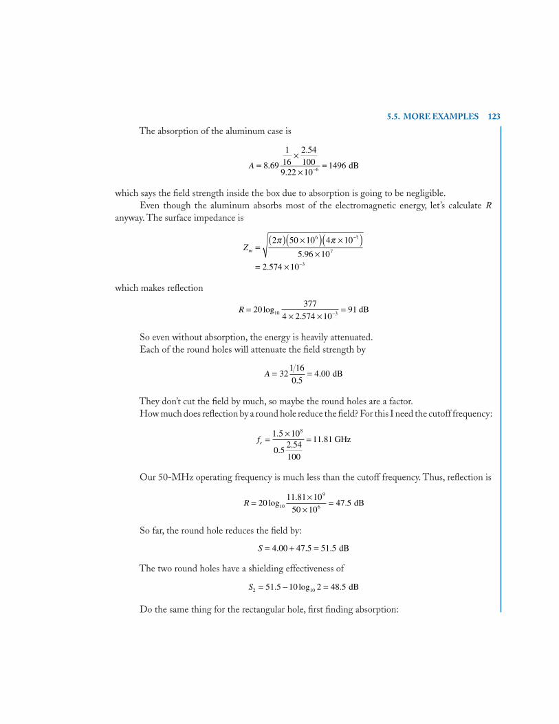
5.5. MORE EXAMPLES 123
The absorption of the aluminum case is
A =×
×=−8 69
116
2 54100
9 22 101496
6.
.
.dB
which says the field strength inside the box due to absorption is going to be negligible.Even though the aluminum absorbs most of the electromagnetic energy, let’s calculate R
anyway. The surface impedance is
Zm =( ) ×( ) ×( )
×= ×
−
−
2 50 10 4 10
5 96 10
2 574 10
6 7
7
3
π π.
.
which makes reflection
R =× ×
=−20377
4 2 574 109110 3
log.
dB
So even without absorption, the energy is heavily attenuated.Each of the round holes will attenuate the field strength by
A = =321 16
0 54 00
.. dB
They don’t cut the field by much, so maybe the round holes are a factor.How much does reflection by a round hole reduce the field? For this I need the cutoff frequency:
fc =×
=1 5 10
0 52 54100
11 818.
..
. GHz
Our 50-MHz operating frequency is much less than the cutoff frequency. Thus, reflection is
R =×
×=20
11 81 10
50 1047 510
9
6log
.. dB
So far, the round hole reduces the field by:
S = + =4 00 47 5 51 5. . . dB
The two round holes have a shielding effectiveness of
S2 1051 5 10 2 48 5= − =. log . dB
Do the same thing for the rectangular hole, first finding absorption:

124 5. ELECTROMAGNETIC COMPATIBILITY
A = =27 31 16
20 85. . dB
Better check reflection, too. The cutoff frequency is
fc =×
=1 5 10
22 54100
2 958.
.. GHz
Again, our operating frequency is well below the cutoff frequency, so reflection at the rectan-gular hole is
R =××
=202 95 10
50 1035 410
9
6log
.. dB
The rectangular hole is worse than the round ones, which should be no surprise, since it’s somuch bigger:
S = + =0 85 35 4 36 3. . . dB
The shielding effectiveness of the rectangular hole is the poorest. Let’s blame that hole forthe entire field inside the box. Then the magnetic flux density inside as determined from the fluxdensity out is
H
B Houtside o
max
max
.
.
==
= ×( )( ) =−
0 073
4 10 0 0737
A/m
μ
π 99 17 10 8. × − Wb/m2
S for the rectangular hole is a decrease in flux density, so the dB relationship is
SB
BdB
B
B
outside
inside
outside
inside
= =20 36 310log .
== =10 65 336 3 20. .
The flux density B inside the box, which is mostly due to the large rectangular hole, is
BB
insideoutside= = × −
65 31 40 10 9
.. Wb/m2
Keep in mind that we’ve used a number of approximations, including some of the formulasthemselves. But these combine to give us an estimate of the field inside. Once we know this, we canjudge whether that is acceptable. If this isn’t enough, we need to improve the shielding to reach ourgoal. A pretty obvious place to start with be somehow screening the large rectangular hole.

5.6. SUMMARY 125
5.6 SUMMARYUnwanted energy is coupled into circuits through capacitive, magnetic, and radiation modes, but nomatter how it gets there, we don’t want it. Our primary methods for keeping this energy out are tochange spacing or orientation, add ground planes, or build shields.
Keeping electromagnetic radiation out makes use of both absorption and reflection. Absorp-tion depends on the thickness of the shielding conductor. Reflection depends on the ratio of thesurface impedance of the shield to that of free space. Holes, which we need for cables and ventilation,also absorb and reflect energy as long as the frequency of the energy is less than the critical frequency.
Note that the work in this chapter is not a rigorous analysis. Our goal is insight into how tokeep interference out.


FORMULAS AND EQUATIONS 127
FORMULAS AND EQUATIONS1. Peak voltage by magnetic-field coupling
VA
rI B AN o= =
μπ
ω ω2
2. Effects of twisting conductors (max. n = 1000)
V V V nO S N= +
3. Shield effectiveness
SV
Vno shield
shield
= 20 10log
4. Effectiveness is sum (in dB) of absorption and reflection
S A R= + in dB
5. Physical constants
6. Absorption with skin depth—t thickness in meter
At
= =8 692
.δ
δωμσ
in dB, skin depth
7. Reflection by shield
RZ
ZZ
mm=
⎛⎝⎜
⎞⎠⎟
= =204
377100
0log ,(dB), Z Ωωμσ
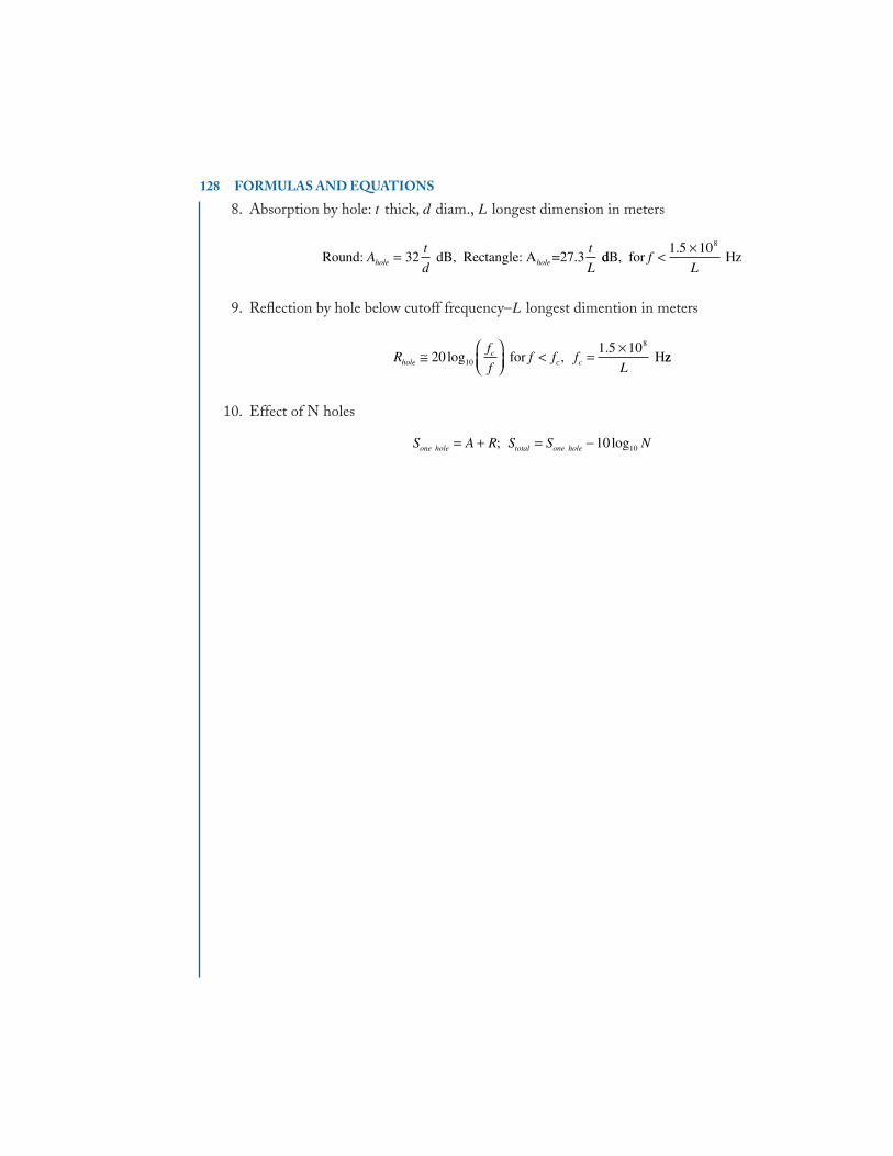
128 FORMULAS AND EQUATIONS
8. Absorption by hole: t thick, d diam., L longest dimension in meters
Round: dB, Rectangle: A =27.3At
d
t
Lhole hole= 32 ddB, for HzfL
<×1 5 108.
9. Reflection by hole below cutoff frequency–L longest dimention in meters
Rf
ff f f
Lholec
c c≅⎛⎝⎜
⎞⎠⎟
< =×
201 5 10
10
8
log ,.
for Hzz
10. Effect of N holes
S A R S S None hole total one hole; log= + = −10 10

129
Author’s Biography
WILLIAM ECCLESBill Eccles has been Professor of Electrical and Computer Engineering at Rose-Hulman Instituteof Technology since 1990 (except for one year at Oklahoma State). He retired in 1990 as Distin-guished Professor Emeritus after 25 years at the University of South Carolina. He founded theDepartment of Computer Science at that university, and served at one time or another as head offour different departments, Computer Science, Mathematics and Computer Science, and Electricaland Computer Engineering, all at South Carolina, and Electrical and Computer Engineering atRose-Hulman. Most of his teaching has been in circuits and in microprocessor systems. He haspublished Microprocessor Systems: A 16-Bit Approach (Addison-Wesley, 1985) and numerous mono-graphs on circuits, systems, microprocessor programming, and digital logic design. In this SynthesisLectures in Digital Circuits and Systems series, Bill has published several texts in this Pragmaticseries, all to introduce electrical topics to non-electrical engineers.
Bill and his wife Trish have two children and four grandchildren. Bill is also a conductor (ap-propriate for an electrical engineer) on the Whitewater Valley Railroad, a tourist line in Connersville,Indiana.
He is a Registered Professional Engineer and an amateur radio operator.


![3.1 - Electrical System, Instruments [OCR]](https://static.fdocuments.us/doc/165x107/577cc3b21a28aba71196e387/31-electrical-system-instruments-ocr.jpg)