PRACTICAL METHODS FOR ASSESSING THE QUALITY OF SUBJECTIVE SELECTION PROCESSES

Laura J. Kornish

Leeds School of Business University of Colorado Boulder

kornish@colorado.edu

Karl T. Ulrich The Wharton School

University of Pennsylvania ulrich@wharton.upenn.edu

June 2016

ABSTRACT

Selection processes are everywhere in business and society: new product development, college

admissions, hiring, and even academic journal submissions. Information on candidates is

typically combined in a subjective or holistic manner, making assessment of the quality of the

process challenging. In this paper, we address the question, “how can we determine the

effectiveness of a selection process?” We show that even if selection is subjective, we can

evaluate the process by measuring an additional audit variable that is at least somewhat

predictive of performance. This approach can be used either with or without observing eventual

performance. We illustrate our methods with data from two commercial settings in which new

product opportunities are selected.

Keywords: selection, selection quality, innovation, new product development, tournaments, idea

evaluation

Acknowledgment: The Mack Center for Technological Innovation at Wharton and the Deming

Center for Entrepreneurship at Leeds provided financial support for this research. We are

grateful for helpful comments on this work from Gerard Cachon, John Lynch, Mike Palazzolo,

Nick Reinholtz, Linda Zhao, and participants at the 11th Annual Product and Service Innovation

Conference.

2

Selection processes are everywhere in business and society. Selections happen in new

product development, college admissions, hiring, and even academic journal submissions. A

selection process is any situation in which there are many candidates and a decision maker is

attempting to select the best ones.

Rarely do organizations know the quality of their selection process. Even if the ideas that

are developed, or the people hired, are tremendously successful, it could be that the remaining

candidates would have been similarly successful, and running controlled experiments investing

in randomly selected candidates would be prohibitively expensive. Assessing the quality of a

selection process is inherently a difficult question. The very information that would be needed

about candidates to determine the quality of the process—how well each one will perform—is

exactly the information that the decision maker is already trying to tap in making the selection.

There is a long stream of literature documenting the superior performance of

“mechanical” (algorithmic or formulaic) over “clinical” (subjective or holistic) decisions (Meehl

1957, Dawes, Faust, and Meehl 1989; Grove and Meehl 1996). Kuncel et al. (2013) performed a

meta-analysis comparing mechanical and clinical approaches in hiring and academic admission

selection decisions. Consistent with previous literature, they find that the mechanical decisions

have much better predictive power. However, holistic decision approaches are entrenched, in

spite of much research showing that they are inferior. Recent research shows that people will

choose a human over an algorithm even when they see the algorithm outperform the human

(Dietvorst, Simmons, and Massey 2015).

The percentage of candidates selected—the nominal selectivity—expresses the intended

exclusivity of the process: selecting 1% of the candidates is of course “more selective” than

selecting 10% of them. However, that nominal selection percentage ignores the uncertainty about

3

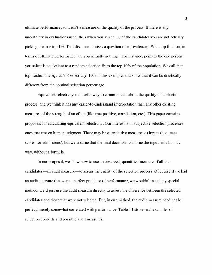
ultimate performance, so it isn’t a measure of the quality of the process. If there is any

uncertainty in evaluations used, then when you select 1% of the candidates you are not actually

picking the true top 1%. That disconnect raises a question of equivalence, “What top fraction, in

terms of ultimate performance, are you actually getting?” For instance, perhaps the one percent

you select is equivalent to a random selection from the top 10% of the population. We call that

top fraction the equivalent selectivity, 10% in this example, and show that it can be drastically

different from the nominal selection percentage.

Equivalent selectivity is a useful way to communicate about the quality of a selection

process, and we think it has any easier-to-understand interpretation than any other existing

measures of the strength of an effect (like true positive, correlation, etc.). This paper contains

proposals for calculating equivalent selectivity. Our interest is in subjective selection processes,

ones that rest on human judgment. There may be quantitative measures as inputs (e.g., tests

scores for admissions), but we assume that the final decisions combine the inputs in a holistic

way, without a formula.

In our proposal, we show how to use an observed, quantified measure of all the

candidates—an audit measure—to assess the quality of the selection process. Of course if we had

an audit measure that were a perfect predictor of performance, we wouldn’t need any special

method, we’d just use the audit measure directly to assess the difference between the selected

candidates and those that were not selected. But, in our method, the audit measure need not be

perfect, merely somewhat correlated with performance. Table 1 lists several examples of

selection contexts and possible audit measures.

4

TABLE 1: EXAMPLES OF SELECTION CONTEXTS

Context Likely Implicit Inputs to Actual Subjective Selection Process

Potential Audit Measures

Product concept selection Judgments about technical feasibility and market attractiveness

Purchase intent survey results from consumers

Collaborator community votes on concepts

Independent evaluation by experts

Primary school teacher hiring Years and nature of training and experience, letters from references, interviews

Results from standardized tests (e.g., Gallup’s TeacherInsight)

Independent review of files by an audit panel

Ratings of classroom observation videos

School admissions Grades, test scores, extracurricular activities, letters from references

Formulaic combination of quantified attributes (e.g., grades, scores, number of leadership positions, years of participation in activities)

Independent review of files by an audit panel

Ratings from multiple alumni interviews

Academic journal submissions Review team and editor assessments of contribution, correctness, and clarity

Assessments from a larger pool of reviewers reading an extended abstract

Independent review of files by an audit review team

Number of downloads of working paper

Our recommendations for the audit measure and its use vary based on the other available

information. First, we consider the case where performance measures (e.g., profit, employee

productivity, student success, paper citations) are available for selected candidates and where the

audit measure mimics the information and process of the original selection (e.g., review of

candidates by similarly qualified people using similar information). Second, we consider the case

where performance measures are available, but the audit measure is not assumed to mimic

closely the original process. In that case, we show how two different audit measures identify

selection quality. Third, we consider the most restrictive case, in which performance measures

are not available. In that case, we require an assumption that the original process and the audit

5

measure have similar predictive power for performance. In each of these three cases, we derive a

specialized formula for translating the available information to an estimate of selection quality,

which we then express as the equivalent selectivity.

Many selection processes have multiple stages, like a tournament (Terwiesch and Ulrich

2009) or a funnel (Chao, Lichtendahl, Grushka-Cockayne 2014). Knowing the quality of a

selection process is essential to making intelligent decisions about the shape of a funnel. The

worse the initial selection process, the more ideas one should advance to the next stage. Knowing

the quality of a selection process is also helpful in tracking the results of interventions designed

to improve that quality (Krishnan and Loch 2005, Bendoly, Rosenzweig, Stratman 2007).

We aspire to a practical method. Our emphasis is on what can realistically be measured to

answer the question of how good a selection process is, given the inherent data limitations. The

next section reviews the related literature. The subsequent section explains equivalent selectivity

and its computation. After that, we present stages of a model with progressive assumptions about

what can be observed and provide methods for estimating the quality of the selection process

from each set of available information. We apply the methods to product concept selection at

Quirky.com and design selection at Threadless.com. The final section concludes.

RELATED LITERATURE

Selection is a key decision in innovation. In a typical product development funnel, ideas

are selected to advance to the next stage for further investment. Scholars have proposed and

validated approaches for evaluating idea quality: Goldenberg, Mazursky, and Solomon 1999,

Goldenberg, Lehmann, and Mazursky 2001, Åstebro and Elhedhli 2006, and Kornish and Ulrich

2014. These studies measure how good the proposed approach is at predicting success of ideas

6

using data on market performance. Our focus in this paper is different: we devise a framework

for evaluating any selection process, even ones lacking a formal model for evaluating the

candidates or a process for measuring the ultimate performance of selected candidates.

The central question in this paper is how to tell how good a selection process is. This

question is closely related to a different question that has received a lot of attention in

psychology and economics: how to measure the relationship between two variables in a sample

shaped by selection. For example, how well does the LSAT predict grades in law school? Or

how well do interviews predict on-the-job performance? The challenge in that question about the

relationship between two variables is that grades and performance are only observed for a non-

random sample of the population. In other words, you only see what the selected candidates, but

not the rejected candidates, achieve.

If the LSAT or the interview were the only basis for admission or hiring, then the

question of measuring the relationship in a systematically selected sample is the same question

we study. However, real selection processes are usually not so mechanical. As Linn (1968)

writes, “the true explicit selection variables are either unknown or unmeasurable.” Sackett and

Yang (2000) concur and say that “[s]election may be on the basis of an unquantified subjective

judgment.”

Many authors have focused on the specific challenge of how to measure the relationships

among variables when the selection variable is relevant to those variables but unmeasured.

Sackett and Yang (2000) reference the work of Olson and Becker (1983) and Gross and

McGanney (1987) for approaches to this challenge. In those works, the key recommendation is

to use the technique from econometrics proposed by Heckman (1979).

7

The Heckman selection model has been shown to be a useful approach for measuring the

relationship between variables when the sample is formed based on information about one or

more of those variables. Heckman (1979) shows that the selection effect acts like an omitted

variable in biasing the results and proposes a method for correcting that bias.

Heckman’s approach was designed to help measure the relationship between an outcome

and a predictor (e.g., wages and years of education). It could also be helpful in estimating the

quality of a selection process, our central question. However, to be useful, we would need to

have a measured variable that predicts selection but that does not also predict outcomes. In

Heckman’s original study, the selection equation models women’s workforce participation and

the outcome equation models wages. Women who would tend to have lower wages are less

likely to be in the workforce, but there are other variables, such as the number of young children

in the home, that predict selection but don’t impact the relationship between wages and

education. The number of young children can serve as that extra variable that identifies the

model.

Strictly speaking, Heckman’s model could separately identify the selection effect from

the overall relationship between the outcome and the focal variable, even without an extra

variable in the selection equation. Without extra variables, the identification relies on the non-

linearity of the residual. However, in practice, the residual is close to linear over much of the

relevant range. The high correlation between the predictor variable and the residual make it

practically impossible to separately identify the two effects (Little, 1985).

Heckman’s original application was not a centralized selection processes with a decision

maker deliberately trying to select the women with the highest wage potential to participate in

the workforce. However, his technique could potentially be relevant to deliberate selection

8

processes, that is, those in which there is a concerted effort to pick the best candidates.

Unfortunately, in a deliberate selection process, it is likely impossible to have an extra variable

that predicts selection but does not predict performance. The decision maker is trying to select

the candidates with the best predicted performance, so if there is an available variable that

predicts performance, the decision maker should already be using it. With no extra variable to

include in the model of selection, it is not practical to use the Heckman selection model. That

conundrum, about the difficulty of identifying variables to use the Heckman model, is our

motivation for proposing methods to assess the quality of subjective selection processes.

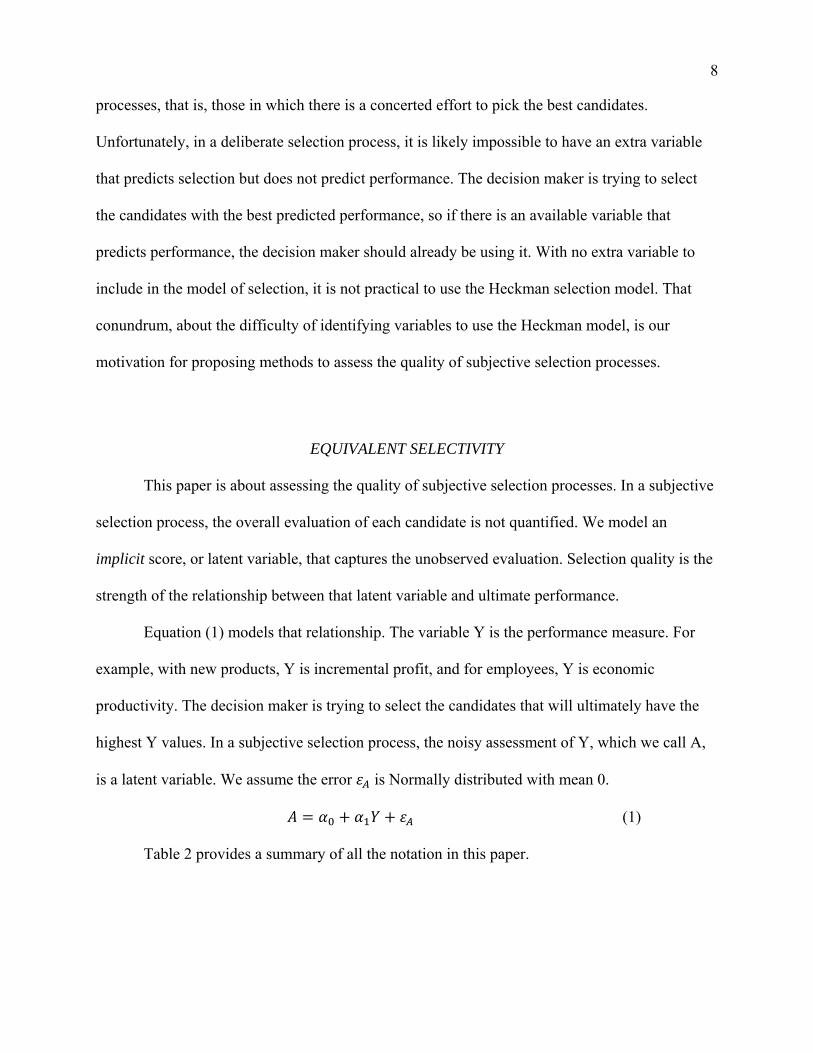
EQUIVALENT SELECTIVITY

This paper is about assessing the quality of subjective selection processes. In a subjective

selection process, the overall evaluation of each candidate is not quantified. We model an

implicit score, or latent variable, that captures the unobserved evaluation. Selection quality is the

strength of the relationship between that latent variable and ultimate performance.

Equation (1) models that relationship. The variable Y is the performance measure. For

example, with new products, Y is incremental profit, and for employees, Y is economic

productivity. The decision maker is trying to select the candidates that will ultimately have the

highest Y values. In a subjective selection process, the noisy assessment of Y, which we call A,

is a latent variable. We assume the error is Normally distributed with mean 0.

(1)

Table 2 provides a summary of all the notation in this paper.

9

TABLE 2: NOTATION

Notation Meaning

Y Candidate ultimate performance (e.g., profit, productivity)

A Implicit score or latent variable that captures the unobserved evaluation used in the selection decision

and Intercept and slope of the relationship between A and Y

Error in the relationship between A and Y

B An audit measure: an observed measure taken on all candidates

and Intercept and slope of the relationship between B and Y

Error in the relationship between B and Y

and SB The mean value of B across all candidates and the standard deviation of B across all candidates

and sB The mean value of B across selected candidates and the standard deviation of B across selected candidates

d Standardized mean difference between B for selected candidates and for all candidates

and Correlation between A and Y, and the correlation between B and Y. More generally represents the correlation between the (possibly unobserved) variables in the subscript

Correlation in the observed samples of B and Y. More generally, r represents the correlation between the observed variables in the subscript

C A second audit measure: an observed measure taken on all candidates

and Intercept and slope of the relationship between C and Y

Error in the relationship between C and Y

k Relative marginal contribution to agreement of shared error compared to shared truth

The correlation between the A and Y, , gives a quantitative measure of how good the

selection process is. A higher means a better, more accurate selection process. But the

correlation alone doesn’t have a natural interpretation for selection. We propose a different

metric, what we call the equivalent selectivity, with a more meaningful interpretation. The

equivalent selectivity answers the question: the mean of what top fraction of performance is

equal to the predicted average performance of candidates actually selected? In Appendix A1, we

compare how equivalent selectivity is related to other, existing measures of classification

accuracy.

10

Figure 1 shows how selection quality (on the horizontal axis) and nominal selection

percentage (each curve in the figure) combine to generate the equivalent selectivity. For

example, with a of 0.3 and a nominal selection percentage of 10% (selecting the perceived

top 10% of the candidates), you are getting performance equivalent to randomly selecting from

the top 67% of candidates. In other words, instead of actually getting the top 10% of candidates,

the mean performance of the selected candidates is equal to the mean of the top two-thirds of the

population of candidates.

The curves in Figure 1 are generated via simulation of candidate values A = Y + ,

where Y are true performance values and are errors, using Normal distributions. By varying

the standard deviation of the error term, we simulate different values of . In each simulation,

the candidates with the highest A values form the selected set, with the exact quantity in the set

determined by the nominal selection percentage. We numerically solve for the percentile of the

Y distribution that equates the mean of the upper tail of that distribution and the mean of the Y

values in the selected set. The equivalent selectivity is the complement of that percentile.

The equivalent selectivity is considerably less selective than the nominal selection

percentage due to a winner’s curse: the top-rated ideas tend to be the ones whose values were

most overoptimistically estimated. The top-rated ideas do tend to have higher performance than

lower-rated ones, but the errors are systemically higher, too. That systematic bias makes the

nominal selection percentage overstate the actual, or equivalent, selectivity, sometimes

dramatically.

11

FIGURE 1: EQUIVALENT SELECTIVITY

This figure shows the equivalent selectivity for a selection process of a certain validity (the horizontal axis, ) and for different nominal selection percentages, ranging from 1% to 50%. The lighter dashed lines illustrate a finding from a personnel selection context: Schmidt and Hunter (1998) report that a measure of general mental ability combined with an evaluation of a work sample has a validity of 0.63. If 10% of candidates are selected, the mean performance of the selected candidates is equal to the top third of the population of candidates.

MODEL

In selection, many candidates are considered and only the best ones are chosen. We

consider the situation where selection is ultimately made based on subjective judgment. We

model that judgment with a latent variable, i.e., one that is implicit and unobserved, as

12

introduced in Equation (1). There may be elements of the selection process that are quantified

and observed (e.g., standardized test scores in admissions or concept testing outcomes in new

product funnels), but we allow for the typical practice of reliance on unquantified human

judgment (Kuncel et al., 2013) in combining those elements. Although we don’t observe ratings

of candidates, we do observe which candidates are selected and which ones are not.

Clearly the observation of what was selected and what was not does not provide enough

information to evaluate how well selections are being made. Therefore, our proposal includes

collecting an audit measure—a measured variable thought to be related to performance, and

therefore selection, for all candidates. The audit measure can be already available and recorded,

captured as part of the candidate consideration process, or it can be obtained after the fact, as part

of the investigation to find out how good the selection process is. Table 1 contains examples of

such audit measures.

We call the audit measure B. Similar to Equation (1), B is a noisy measure of Y

(performance), linearly related to Y, with Normally distributed and mean-zero error .

(2)

The question we address in this work is how we can get a good estimate of the relationship

between A and Y ( ) given that we don’t observe A at all and at best we only observe Y for

candidates with the highest A.

A linchpin in this analysis is a relationship among four correlations, as shown in the

result below.

Result 1. For the model in Equations (1) and (2), the relationship among the predictive validity

of A, ; the predictive validity of B, ; the correlation between the errors, ; and the

correlation between A and B, , is

13

1 1 (3)

We derived this equation from the definition of correlation and the formulas for the coefficients

and . See Appendix A2 for the derivation.

Equation (3) shows the key challenge in understanding how good a latent selection

variable is by using a related observed audit measure. On the one hand, the latent variable and

the audit measure may agree because they are both good predictors of future success of

candidates, i.e., and are both positive. On the other hand, the two measures may agree

because they are relying on the same limited set of information and drawing the same incorrect

conclusions, i.e., and may be zero, but is positive.

How can we make the most informed estimate of ? If we knew the other three

correlations in Equation (3), we could find the value of , but we do not know them. Our

contribution in this paper is to explain how we can combine reasonable assumptions with

observations to learn about , the variable we ultimately care about.

First consider . This is a measure of the agreement of the latent selection variable and the

observed audit measure. We do observe something that is useful for estimating . To measure

agreement between A and B, we can calculate how different B is, on average, between the

selected group and the whole population. We use the normalized difference between two groups

(like Cohen’s d):

,

where is the mean value of B in the selected group, is the estimate of the mean value

of B in the whole population, and is an estimate of the standard deviation of B for the whole

population. Appendix A3 shows the exact formula to infer from d if we assume that A and B

are Bivariate Normal; is the biserial correlation (Thorndike 1949). We use that relationship

14

in this paper. For more generality, one could simulate to derive the correspondence between d

and for other distributional forms.

In considering and , first, we examine the case in which Y is observed, and then

we turn to the most restrictive case, in which Y is not observed.

PROPOSED METHODS AND APPLICATION: OBSERVED PERFORMANCE

In many cases, the measure of performance Y will be observed for the selected

candidates. In this section, we show how to make use of that information to improve our estimate

of . We present two different approaches: one in which the audit measure B mimics the

original latent selection variable A, and one in which we do not require that.

Observed Audit Measure B Mimics Original Selection Process

The first way to use Y to estimate is to develop an audit measure B that has similar

predictive power to A. One way to achieve this matching is to use a B that mimics A. Although

A may not have been quantified or documented, some details about the information used and the

process used for selection may be known. Using the same information and to the extent possible,

the same process, quantify B. Then use that variable to estimate , which serves as an estimate

of .

Consulting Table 1, the examples of audit measures that involve independent reviews of

the information in files by separate (and presumably equally, or nearly equally, qualified) people

would meet the equal-predictive-power criterion.

Note that we do not require that A and B agree (high ), simply that they have similar

predictive power. If they are both noisy signals, then we can have but low .

15

If we do observe B and Y in the selected sample, how do we get an estimate of ?

Sackett and Yang (2000) review the approaches for correcting an observed correlation in a

selected sample to estimate the correlation over the entire population of the two variables,

referencing Thorndike (1949), and in turn Pearson (1903). As Sackett and Yang (2000) note, the

Thorndike Case 2 correction is considered the standard correction. We show it in Equation (4),

where is the correlation between B and Y in the observed sample, is the standard

deviation of B in the whole population, and is the standard deviation of B in the selected

sample.

⁄ (4)

Unfortunately, Equation (4) is not an exact correction for our purposes because B is not

the selection variable (and A, which is, is not observed). Even though the conditions for Case 2

are not strictly met, our simulations reveal that the estimates are very good across all parts of the

parameter space. Appendix A4 shows the results of the simulations: the simulated estimate of

is very close to the true value across the whole parameter space.

In summary, we can obtain an estimate of if we can mimic the information and

process implicit in A, but in the imitation, quantify and document it and create an audit measure

B. Once we have done that, we measure the correlation of B and Y in the selected sample ( )

and use Equation (4) to infer the correlation of B and Y ( ) in the full population. The value of

serves as our estimate of .

Selection Process is Too Opaque to be Properly Mimicked

In the previous subsection, we show how to estimate the quality of a selection process

( ) if B mimics A. More generally, though, there are selection processes that rely heavily on

16

tacit subjective judgment, undocumented and opaque. It may be unclear what information was

used in the selection process, or how it was applied. In those cases, it would be hard to create an

audit measure B to mimic A, therefore, we would not want to assume that . Dropping

that assumption, we need an additional source of information, namely something to help us

estimate .

We still rely on an audit measure B, as in Equation (2). Unlike the previous approach,

though, instead of attempting to have B be a replication of A, it should be the best attempt of a

predictor of Y. The audit measure B, compared to A, may be a better or worse predictor of Y. In

addition to B, we also need a second observed variable in the selected sample, which we call C:

(5)

As in Equations (1) and (2), we assume that is Normal with mean zero. In Table 1, we show

multiple possible audit measures for each context. From each list, the one that is thought to be

the best predictor of Y should serve as B, and the one that most closely replicates the original

selection process should serve as C. For example, in new product concept selection, purchase

intent survey results from consumers—which have been shown to be predictive of market

behaviors (Kornish and Ulrich 2014)—are a good source for B. Many companies rely on a small

group of insiders to screen the initial large set of ideas (dozens or hundreds) down to a much

smaller set (Magnusson et al. 2016), so evaluations by a new set of experts are a good source for

C.

The role of the second audit measure C is to provide information about error correlation.

Observing B, C, and Y in the selected sample, we calculate the correlation between and in

that sample (which we call ). We are not relying on C being an exact reproduction of the

original latent selection variable A, because we are not basing our estimate of directly on our

17

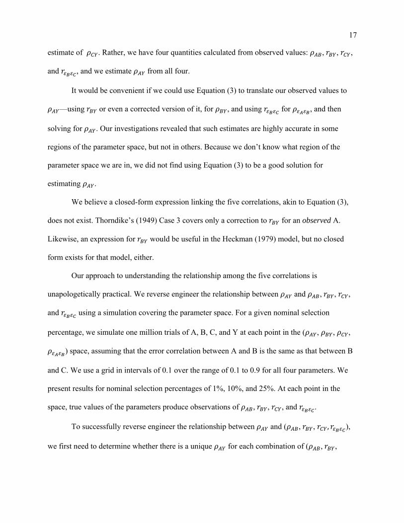
estimate of . Rather, we have four quantities calculated from observed values: , , ,

and , and we estimate from all four.

It would be convenient if we could use Equation (3) to translate our observed values to

—using or even a corrected version of it, for , and using for , and then

solving for . Our investigations revealed that such estimates are highly accurate in some

regions of the parameter space, but not in others. Because we don’t know what region of the

parameter space we are in, we did not find using Equation (3) to be a good solution for

estimating .

We believe a closed-form expression linking the five correlations, akin to Equation (3),

does not exist. Thorndike’s (1949) Case 3 covers only a correction to for an observed A.

Likewise, an expression for would be useful in the Heckman (1979) model, but no closed

form exists for that model, either.

Our approach to understanding the relationship among the five correlations is

unapologetically practical. We reverse engineer the relationship between and , , ,

and using a simulation covering the parameter space. For a given nominal selection

percentage, we simulate one million trials of A, B, C, and Y at each point in the ( , , ,

) space, assuming that the error correlation between A and B is the same as that between B

and C. We use a grid in intervals of 0.1 over the range of 0.1 to 0.9 for all four parameters. We

present results for nominal selection percentages of 1%, 10%, and 25%. At each point in the

space, true values of the parameters produce observations of , , , and .

To successfully reverse engineer the relationship between and ( , , , ),

we first need to determine whether there is a unique for each combination of ( , ,

18

, ). Regrettably, there is not a unique relationship. Appendix A5 illustrates a

counterexample.

Because there is not a one-to-one mapping from the other four parameters to , there

can’t be an unambiguous relationship linking the observed quantities to . However, for much

of the parameter space, there is a unique relationship between the four other parameters and .

In other words, the iso- surfaces do not intersect. In addition, the surfaces, while not linear,

appear to be monotonic, suggesting that approximations based on simple functional forms may

be reasonable. The intersections happen in one corner of the space: low and high . We

therefore study the relationship excluding that corner. Those restrictions make sense intuitively.

We can’t expect to use B (the audit measure) to calibrate A (the latent variable representing the

original selection process) if B itself has essentially no predictive power for performance. And

we can’t expect to use B to calibrate A if the high error correlation makes the two measures

indistinguishable. In the analysis below, we restricted the range based on observed values

0.25 and 0.5. We chose these cut-offs recognizing that the tighter the restriction, the

better the model will fit, but the lower the chance that we can use it. (The results are not highly

sensitive to the exact cut-offs.)

To find the relationship between and , , , and in the restricted range,

we regress the simulated on the other terms and their two-way interactions. Table 3 shows

the regression coefficients for three nominal selection percentages. The R2s are very high, above

90% in all three cases.

19

TABLE 3: REGRESSION RESULTS FOR PREDICTING WITH OBSERVED B, C, and Y

Select Top 1%

Select Top 10%

Select Top 25%

Variable

Coefficients (Standard Error)

Constant 0.291*** (0.015)

0.263*** (0.015)

0.240*** (0.013)

2.295*** (0.032)

2.565*** (0.032)

2.714*** (0.030)

-0.239*** (0.021)

-0.216*** (0.021)

-0.160*** (0.019)

-0.002 (0.017)

-0.002 (0.017)

-0.028* (0.015)

-4.149*** (0.061)

-4.342*** (0.057)

-4.403*** (0.050)

-1.609*** (0.045)

-1.940*** (0.044)

-2.194*** (0.040)

0.023 (0.027)

0.013 (0.027)

0.024 (0.025)

1.009*** (0.057)

1.075*** (0.056)

1.302*** (0.051)

0.084*** (0.020)

0.086*** (0.019)

0.076*** (0.018)

3.379*** (0.065)

3.658*** (0.060)

3.660*** (0.054)

-0.288*** (0.042)

-0.269*** (0.039)

-0.151*** (0.036)

N 2844 2751 2679

R2 0.93 0.94 0.95

Adj. R2 0.93 0.94 0.95

*** p < 0.01, ** p < 0.05, * p<0.1

Notes: Regression results for translating observed values of ( , , , ), when the restrictions are met ( 0.25 and 0.5), into an estimate of , for a given nominal selection percentage.

From these results, we notice that the largest simple effects come from , with a strong

positive effect on ; and , with a strong negative effect on . Of the six interaction

terms, the largest effects are from (negative) and (positive). All the terms

including are either not significant or show relatively weak impact compared to other terms

20

in the estimation. The variable C (the second audit measure) was introduced to provide some

basis for estimating , and we do see strong effects of , as we would expect from

Equation (3), but the doesn’t provide much information directly about .

In summary, we can obtain an estimate of if we have an audit measure B with non-

negligible predictive power for Y greater than 0.25, or so) and a second audit measure C

with substantial independent information from B ( less than 0.5, or so). With those

variables, we obtain estimates of the agreement of B with the original selection ( ), and

measure correlations , ,and . We plug those measurements into the appropriate model

from Table 3, based on the nominal selection percentage, to calculate the estimate of . We

can translate the correlation into an equivalent selectivity—a top fraction of the distribution

on performance—using the relationships expressed in Figure 1.

Application

We apply this method to data from the product-development company Quirky.com.

Quirky had a website at which community members submitted ideas for household products, and

some of the products were selected, developed, and sold in the online store. The Quirky products

are used in different rooms of the house, for example kitchen appliances, bathroom organizers,

and office gadgets. Our question is, “how good is Quirky at selecting concepts?”

The key elements of the data set are as follows.

A random sample of 100 “raw ideas” submitted to the idea contests from the site. Raw

ideas comprise short text descriptions, and in some cases, visual depictions.

A set of 149 raw ideas that were selected to be developed into products. This set

comprises every product Quirky selected for commercialization as of February 2013.

21

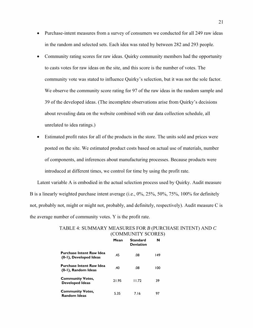
Purchase-intent measures from a survey of consumers we conducted for all 249 raw ideas

in the random and selected sets. Each idea was rated by between 282 and 293 people.

Community rating scores for raw ideas. Quirky community members had the opportunity

to casts votes for raw ideas on the site, and this score is the number of votes. The

community vote was stated to influence Quirky’s selection, but it was not the sole factor.

We observe the community score rating for 97 of the raw ideas in the random sample and

39 of the developed ideas. (The incomplete observations arise from Quirky’s decisions

about revealing data on the website combined with our data collection schedule, all

unrelated to idea ratings.)

Estimated profit rates for all of the products in the store. The units sold and prices were

posted on the site. We estimated product costs based on actual use of materials, number

of components, and inferences about manufacturing processes. Because products were

introduced at different times, we control for time by using the profit rate.

Latent variable A is embodied in the actual selection process used by Quirky. Audit measure

B is a linearly weighted purchase intent average (i.e., 0%, 25%, 50%, 75%, 100% for definitely

not, probably not, might or might not, probably, and definitely, respectively). Audit measure C is

the average number of community votes. Y is the profit rate.

TABLE 4: SUMMARY MEASURES FOR B (PURCHASE INTENT) AND C (COMMUNITY SCORES)

Mean Standard Deviation

N

Purchase Intent Raw Idea (0-1), Developed Ideas

.45 .08 149

Purchase Intent Raw Idea (0-1), Random Ideas

.40 .08 100

Community Votes, Developed Ideas

21.95 11.72 39

Community Votes, Random Ideas 5.35 7.16 97

22

From Table 4, we derive the standardized mean difference between the selected group

and the population, d = (.45-.40)/.08 = .63. Quirky selected about 1% of the products submitted,

so the implied is 0.24 (using the biserial correlation formula in Appendix A3). Using the

performance measure (Y) as the natural log of the profit rate, we find the correlation between

purchase intent score (B) and logged profit rate (Y) to be 0.27 in the observed sample.

With the community scores as the second audit measure C, is 0.06 in the observed

sample. We use C to help get an estimate of the error correlation between A and B; therefore, a

good C is one that is strongly related to A in some way. With that criterion, the community

scores are a good choice. Although not part of the model we are estimating, we observed that

using C, the d (standardized mean difference between the selected group and the population) is

2.32. That d implies a of 0.87 for a selection rate of 1% (using the biserial correlation

formula in Appendix A3). Table 4 shows that that the standard deviation of the community

scores for the selected ideas is higher than the standard deviation of the population. This supports

the thought that the community score is not the explicit selection criterion; if it were, the

standard deviation in the set of random ideas would most likely be bigger than the standard

deviation in the set of developed ideas. However, the d of 2.32 tells us the community scores are

an important part of the selection.

Finally, the error correlation—the correlation between residuals from Equation (5) and

those from Equation (2)— in the observed sample is 0.23.

Using the model estimated for the nominal selection percentage of 1%, as shown in Table

3, we estimate as -0.02, essentially zero. In other words, it is as if Quirky were randomly

selecting ideas from its pool of submissions. Of course, this value of is a point estimate.

Using the standard error of the regression (0.064), the 95% confidence interval for is (-0.14,

23

0.11). Consulting Figure 1, the equivalent selectivity is at least 90%. The selection process is at

best weakly predictive of success.

Many of the ideas that Quirky developed were very successful. However, our analysis

cautions us from attributing that success to their selection process. The low value of the

correlation between community scores and performance that we observed ( 0.06) didn’t

automatically dictate that Quirky’s selection process was weak. In fact, if the selection process

were highly accurate, then there could be severe attenuation of the relationship between C and Y

due to restriction of range (Sackett and Yang 2000). However, we conclude that that severe

attenuation is not at play here: instead, the low value of accurately reflects a selection process

that is not highly predictive of profit performance.

PROPOSED METHOD AND APPLICATION: UNOBSERVED PERFORMANCE

In some cases, performance Y is not observed, even for the selected candidates. Why

would Y be unobserved? In studies of the validity of admissions testing, the performance

variable is often first-year GPA. Is this really the ultimate performance measure that one is

hoping to maximize in a highly tuned admissions process? Probably not. Ultimate performance

criteria like “student success” are hard to define and measure. In the case of product concept

selection, profits associated with each new product would be a pretty good measure of

performance. However, even in that straightforward case, true performance would be long-term

incremental profit in the product portfolio. The ideal long-term time frame makes measurement

hard and the idea of incremental profit makes it even harder.

Admittedly, this minimal-data scenario is a very restrictive case. Our task in this setting is

to make a reasonable estimate of having an observation-derived estimate of . We have

24

three unknowns ( , , and ) and only one equation, Equation (3), relating them.

Clearly there isn’t a single solution to the equation. Our estimation proposal relies more on

assumptions about the relative sizes of effects than the previous proposal with observed Y.

Method

To estimate , we want to use an audit measure B that is reasonable to assume has the

same predictive power as A, . We discussed that assumption earlier, in the first case

we presented. With equal predictive power, we simply need an assumption about the relative

contribution to the observed agreement of shared error vs. shared truth.

We examine the family of assumptions that the marginal contribution of shared error is k

> 0 times that of shared truth. Solving for as a function of gives the following result

(proven in Appendix A6).

Result 2. For the model in Equations (1) and (2), if and ∗

, then

1 1 (6)

Figure 2 shows the relationship in Equation (6) for three different values of k. The middle

solid line shows the relationship for k = 1, when the two contributions are equal. The top solid

line in Figure 2 shows when the effect of shared error is half that of shared truth, and the bottom

solid line shows the opposite, the effect of shared error is twice that of shared truth.

The next step is to develop a reasonable range for k. Shared error comes from common

elements of A and B that are unrelated to Y. Common elements can be response formats,

misconceptions or surprises, or biases related to the way the information is presented. For

25

example, if a sketch of an idea from Quirky looks professional, that may bias the evaluation

upward, compared to one that looks amateurish, in both the Quirky process and our consumer

surveys.

FIGURE 2: INFERRING FROM AGREEMENT BETWEEN A AND B WHEN Y IS

UNOBSERVED

Estimates of as a function of the observed agreement between A and B (expressed as the correlation ), assuming . The constant k captures the relative marginal contribution of shared error compared to shared truth.

Starting with Campbell and Fiske (1959), many studies in marketing, management, and

psychology quantify the magnitude of the “common methods bias.” Bagozzi and Yi (1991)

examine methods for measuring it. More recently, Podsakoff et al. (2012) summarize the

findings about the size of the bias. Their Table 1 shows the estimated percentage of variance

explained by methods, “traits” (or truth, in our framework), and random error in five meta-

26

analyses. The k values for the five studies cited in Podsakoff et al. (2012) range from 0.86 (for

the Lance et al. 2010 paper, the one that is most skeptical about the severity of common method

bias) to 1.33 (for Doty and Glick, 1998). Based on these studies, we conclude that 1 is a

reasonable point estimate for k: the marginal effects of shared error and shared truth have been

shown to carry approximately equal weight in generating agreement.

In summary, we can obtain an estimate of if we can mimic the information and

process implicit in A, but in the imitation, quantify and document it and create an audit measure

B. For examples of such audit measures, see Table 1, where we show examples of measures that

involve independent reviews of information by separate and similarly qualified people. We

estimate the correlation between A and B from the standardized mean B difference between the

selected candidates and the whole population. We use an estimate or a range to represent the

relative marginal contribution (k) of shared error and shared truth and solve for from

Equation (6).

Application

To illustrate the use of this proposed method, we collected data from the company

Threadless.com. Threadless has a website at which community members submit designs, then

some of the designs are selected, printed on t-shirts and other products such as cell-phone cases,

and sold in the online store. Threadless runs regular, themed competitions for the designs, for

example Greek and Roman Mythology, Original Comics, and Landscapes. King and Lakhani

(2013) cite Threadless as an example of success of open innovation, in which the crowd

generates the designs and also provides input on selection.

27

Our question is, “how good is Threadless at selecting designs?” by which we mean how

effectively does the company select those designs that would have the highest sales if sold in

their online store? As outsiders evaluating their process, we don’t observe their sales, thus this is

an instance of an application in which Y is not observed.

The key elements of the data set are as follows.

For each of 10 separate, themed contests or batches, we observe the complete set of

winning designs, i.e., the ones selected to be printed on products and sold. Each contest

had 1-3 winning designs.

We draw a random sample of 70 designs that were not selected as winners from each of

the 10 contests. Each contests attracted between 160 and 575 submissions. The designs

are all visual depictions.

We gather ratings, independent from the Threadless platform, from over 100 people for

each of the 718 designs (the winning ones plus the random samples). These ratings use a

scale of 1 to 3: unattractive, neither unattractive nor attractive, and attractive. We used

Amazon’s Mechanical Turk platform to collect these ratings.

The latent variable A represents the actual selection process used by Threadless. The audit

measure B is our independent ratings of each design, obtained from a panel of potential

consumers. In making our estimate, we are assuming that our process has about the same

predictive power as Threadless’ process, . Threadless uses some combination of

community input and managerial judgment to select their designs. On the one hand, they have

more knowledge about their market than we use in our B (suggesting ), but on the

other hand, our B uses similar data but with a mechanical approach, which has been shown to be

superior to a subjective decision (suggesting ).

28

Table 5 shows the summary metrics for the ratings for each contest. Across the 18 winning

designs, the mean rating is 2.18. Across all 3069 designs (winners and the entire population of

non-winners, not just our sample of 718), we estimate the mean rating as 1.99 and the standard

deviation as 0.284, resulting in a d (standardized mean difference between the selected and

whole populations) of 0.67. With the overall selectivity of 18/3069, or 0.59%, a d of 0.67 implies

a of 0.236 (Appendix A3).

TABLE 5: RESULTS FROM 10 THREADLESS CONTESTS

Contest Theme N

Entries N

Winners

Mean Rating of

Winner(s)

Mean Rating of 70 Non-Winners

1. Mythology 229 2 2.09 1.95

2. Massive Design 424 1 1.99 1.97

3. Power Rangers 246 1 2.05 2.02

4. Original Comics 214 1 2.11 1.96

5. Landscapes 244 3 2.46 2.09

6. Doodles 529 2 2.12 1.96

7. B&W Photography 575 1 2.38 2.00

8. Crests 216 3 2.17 2.02

9. Original Cartoons 232 3 2.02 1.95

10. Conspiracy Theories 160 1 2.36 1.96

With an observed value of 0.236, the maximum possible value of k (relative

marginal contribution of shared error and shared truth) is 1.31: at that value of k, the estimate of

is 0. Using a range of k from 1 to that maximum, our estimated range for is 0 to 0.355.

To put that in context, even though Threadless is selecting less than 1% of the designs, the

winning designs are as good, on average, as if they had been randomly selected from at best the

top 40% (and at worst totally at random). That range is the range of equivalent selectivity. See

29

Figure 1. Given the uncertainty, the decision process is dramatically less selective than the

nominal selection percentage of 0.59%.

Although we do not have market results on the winning designs in this Threadless

application, such information would be available to an insider. We use this application as an

example of how to estimate selection quality when performance is unobserved for any reason.

That reason may be that true performance is hard to define or measure, or that it plays out over a

long time horizon. Industry analysts, investors, or competitors all may be interested in the quality

of a selection process, and would naturally be unable to observe performance measures.

We cover this most restrictive case of unobserved Y to show that even in this case, there

is a reasonable process to follow to assess the quality of the selection process.

CONCLUSIONS

Estimating the quality of a selection process is an inherently challenging task. The

decision maker is already exerting his best effort to evaluate the candidates. If he knew exactly

how well he was doing, he could do the job perfectly. In this paper, we have proposed methods

to use information outside of the original selection process to calibrate how well the process

works. Table 6 summarizes those methods.

Knowing the quality of a selection process is especially important when the selection is a

first stage of a multi-stage funnel (Gross 1972, Bateson et al. 2014) or tournament (Dahan and

Mendelson 2001, Terwiesch and Ulrich 2009), where a large set of candidates is winnowed

down. In such settings, knowing the accuracy of the first stage dictates the optimal number of

candidates to advance for further consideration. The optimal number of candidates to advance

can be drastically different depending on the accuracy of the first stage. In Appendix A7, we

30

describe a scenario for which the optimal number of candidates to advance to the second stage

drops from 28 when .02 to 19 when .24 to 12 when .45.

TABLE 6: SUMMARY OF PROPOSED APPROACHES What is observed? What is assumed? What to do?

Which candidates are selected Audit measure B on all candidates Performance Y for selected candidates

Calculate and use use traditional restriction of range correction, Equation (4).

Which candidates are selected Audit measure B on all candidates Audit measure C and performance Y for

selected candidates

Calculate , , , and use coefficients for appropriate model from Table 3.

Which candidates are selected Audit measure B on all candidates

estimate of k (relative marginal

contribution to agreement of error vs. truth)

Calculate and use Equation (6).

As Van den Ende et al. (2015) note, “the quality of selection suffers because good ideas

need attention and consideration, which becomes virtually impossible [with] high numbers” (p

482). It is important to acknowledge the winner’s curse—that the candidates deemed best have

the biggest overestimates—and not narrow the funnel too quickly.

Our proposals progress from more observed data to less, with a trade-off between

assumptions and data requirements. At each step, the methods are pragmatic about what data are

available or can be collected. Studies like that of Dahan et al. (2010) and Dahan et al. (2011),

that demonstrate the predictive power of new ways of forecasting the value of new product

concepts, are a complement to our inquiry.

Our approach is intended to be practical in its simplicity, but of course there are caveats

in its application. The first caveat is that there may be omitted variables from Equations (1) and

(2). This is particularly problematic if A and B both measure something related to performance Y

but are orthogonal to each other. If Y is unobserved, our analysis will incorrectly show that A is

31

uncorrelated with performance. One would hope that a process (implicitly) governed by A

doesn’t have a conspicuous and impactful omission. But if it does, then B should not be focused

on that omission. Such a B would not be useful for assessing the quality of the selection process.

A second caveat is that we have made specific distributional and functional assumptions.

In particular, our analysis uses assumptions about normality and linearity. The central intuition

that agreement between A and B comprises shared truth and shared error survives relaxation of

the distributional assumptions, but the actual decomposition will be different for different

assumptions.

Finally, we note that our approaches are most relevant in contexts like innovation where

there is no concern of “yield,” i.e., offers being accepted. In selection processes involving

people, such hiring and admissions, selection might take on more of a matching perspective and

less of the identify-the-best perspective that we analyze here.

32

REFERENCES

Åstebro, Thomas and Samir Elhedhli. (2006) “The Effectiveness of Simple Decision Heuristics:

Forecasting Commercial Success for Early-Stage Ventures,” Management Science, 52 (3), 395-

409.

Bagozzi, Richard P. and Youjae Yi. (1991) “Multitrait-Multimethod Matrices in Consumer

Research,” Journal of Consumer Research, 17 (4), 426-439.

Bateson, John E.G., Jochen Wirtz, Eugene Burke, and Carly Vaughan. (2014)"Psychometric

sifting to efficiently select the right service employees," Managing Service Quality, 24 (5) 418 –

433.

Bendoly, Bendoly, Eve D. Rosenzweig, and Jeff K. Stratman. (2007) “Performance Metric

Portfolios: A Framework and Empirical Analysis,” Production and Operations Management, 16

(2), 257-276.

Campbell, Donald T. and Donald W. Fiske. (1959) “Convergent and Discriminant Validation by

the Multitrait-Multimethod Matrix,” Psychological Bulletin, 56 (2), 81-105.

Chao, Raul O., Kenneth C. Lichtendahl Jr., Yael Grushka-Cockayne. (2014) “Incentives in a

Stage-Gate Process,” Production and Operations Management, 23 (8), 1286–1298.

Dahan, Ely, Adlar J. Kim, Andrew W. Lo, Tomaso Poggio, and Nicholas Chan. (2011)

“Securities Trading of Concepts (STOC),” Journal of Marketing Research, 48 (3), 497-517.

——— and Haim Mendelson. (2001) “An Extreme Value Model of Concept Testing,”

Management Science, 47 (1), 102-116.

33

——— , Arina Soukhoroukova, and Martin Spann. (2010) “New Product Development 2.0:

Preference Markets—How Scalable Securities Markets Identify Winning Product Concepts and

Attributes,” Journal of Product Innovation Management, 27, 937–954.

Dawes, Robyn M. (1979) “The Robust Beauty of Improper Linear Models in Decision Making,”

American Psychologist, 34 (7), 571-582.

———, David Faust, and Paul E. Meehl. (1989) “Clinical Versus Actuarial Judgment,” Science,

243, 1668-1674.

Dietvorst, Berkeley, Joseph Simmons, and Cade Massey. (2015) “Algorithm Aversion: People

Erroneously Avoid Algorithms After Seeing Them Err,” Journal of Experimental Psychology:

General, 144 (1), 114-126.

Doty, D. H. and W. H. Glick. (1998) “Common methods bias: Does common methods variance

really bias results?” Organizational Research Methods, 1, 374–406.

Goldenberg, Jacob, Donald R. Lehmann, and David Mazursky. (2001) “The Idea Itself and the

Circumstances of Its Emergence as Predictors of New Product Success,” Management Science,

47 (1), 69-84.

———, David Mazursky, and Sorin Solomon. (1999) “Toward Identifying the Inventive

Templates of New Products: A Channeled Ideation Approach,” Journal of Marketing Research,

36 (2), 200-210.

Gross, Alan L. and Mary Lou McGanney (1987) “The Restriction of Range Problem and

Nonignorable Selection Processes,” Journal of Applied Psychology, 72 (4), 604-610.

Gross, Irwin. (1972) “The Creative Aspects of Advertising,” Sloan Management Review, 14 (1),

83-109.

34

Grove, William M. and Paul E. Meehl. (1996) “Comparative Efficiency of Informal (Subjective,

Impressionistic) and Formal (Mechanical, Algorithmic) Prediction Procedures: The Clinical–

Statistical Controversy,” Psychology, Public Policy, and Law, 2, 293–323.

Hand, David J. (2012) “Assessing the Performance of Classification Methods,” International

Statistical Review, 80 (3), 400-414.

Heckman, James J. (1979) “Sample Selection Bias as a Specification Error,” Econometrica, 47

(1), 153-161.

King, Andrew and Karim R. Lakhani. (2013) “Using Open Innovation to Identify the Best Ideas”

Sloan Management Review, 55 (1), 41-48.

Kornish, Laura J. and Karl T. Ulrich. (2014) “The Importance of the Raw Idea in Innovation:

Testing the Sow’s Ear Hypothesis,” Journal of Marketing Research, 51 (1), 14-26.

Krishnan, V. and Christoph H. Loch. (2005) “A Retrospective Look at Production and

Operations Management Articles on New Product Development,” Production and Operations

Management, 14 (4), 433-441.

Kuncel, Nathan R., David M. Klieger, Brian S. Connelly, and Deniz S. Ones. (2013)

“Mechanical Versus Clinical Data Combination in Selection and Admissions Decisions: A Meta-

Analysis,” Journal of Applied Psychology, 98(6), 1060–1072.

Lance, Charles E., Bryan Dawson, David Birkelbach, and Brian J. Hoffman. (2010) “Method

Effects, Measurement Error, and Substantive Conclusions,” Organizational Research Methods,

13 (3), 435-455.

Linn, Robert L. (1968) “Range Restriction Problems in the Use of Self-Selected Groups for Test

Validation,” Psychological Bulletin, 69 (1), 69-73.

35

Little, Roderick J. A. (1985) “A Note About Models for Selectivity Bias,” Econometrica, 53 (6),

1469-1474.

Magnusson, Peter R., Erik Wästlund, and Johan Netz. (2016) “Exploring Users’ Appropriateness

as a Proxy for Experts When Screening New Product/Service Ideas,” Journal of Product

Innovation Management, 33 (1), 4–18.

Meehl, Paul E. (1957) “When Shall We Use Our Heads Instead of the Formula?” Journal of

Counseling Psychology, 4 (4), 268-273.

Olson, C. A., and B. E. Becker. (1983). “A proposed technique for the treatment of restriction of

range in selection validation,” Psychological Bulletin, 93, 137-148.

Pearson, K. (1903) “Mathematical contributions to the theory of evolution—XI. On the influence

of natural selection on the variability and correlation of organs,” Philosophical Transactions,

CC.-A 321, 1-66.

Podsakoff, Philip M., Scott B. MacKenzie, and Nathan P. Podsakoff. (2012). “Sources of

Method Bias in Social Science Research and Recommendations on How to Control It,” Annual

Review of Psychology. 63, 539–69.

Sackett, Paul R. and Hyuckseung Yang (2000). Correction for Range Restriction: An Expanded

Typology Journal of Applied Psychology. 85 (1), 112-118.

Schmidt, Frank L. and John E. Hunter. (1998) “The Validity and Utility of Selection Methods in

Personnel Psychology: Practical and Theoretical Implications of 85 Years of Research Findings,”

Psychological Bulletin, 124(2), 262-274.

Terwiesch, Christian and Karl T. Ulrich. (2009) Innovation Tournaments: Creating and

Selecting Exceptional Opportunities. Boston: Harvard Business Press.

36

Thorndike, Robert L. (1949) Personnel selection: Test and measurement techniques. New York:

Wiley.

Van den Ende, Jan, Lars Frederiksen, and Andrea Prencipe. (2015) “The Front End of

Innovation: Organizing Search for Ideas,” Journal of Product Innovation Management, 32 (4),

482–487.

37

APPENDICES

A1: Comparing Equivalent Selectivity to Other Measures of Classification Accuracy

Comparing equivalent selectivity to other measures of classification accuracy (Hand

2012), we conclude that the correlation dictates not just equivalent selectivity, but also the

overall correct classification rate and the true positive rate. Given those relationships, it follows

that there exist mappings between overall correct classification rate and equivalent selectivity

and between true positive rate and equivalent selectivity. The overall correct classification rate,

however, is not a useful way to express the quality of a selection process when the nominal

selection percentage is low. With a low nominal selection percentage, like 1%, the correct

classification rate is close to 100% no matter how high or low the correlation is: almost every

candidate is correctly classified as not among the best. The true positive rate is more

discriminating, especially when the nominal selection percentage is low. However, we believe

our proposed measure, the equivalent selectivity, has an easier interpretation than the true

positive rate. The equivalent selectivity is a percentage of the whole candidate pool, making it

comparable to the nominal selection percentage itself. In contrast, the true positive rate is a

percentage of only the selected candidates.

A2: Derivation of Equation (3) in Result 1

Using the model in Equations (1) and (2) we derive the correlation of and , .

,

,

, ,

The formulas for the coefficients and are given below.

, ⁄ ⁄ ⁄ .

38

, ⁄ ⁄

Plugging those in, 2 1 2 2 1 2 1 2 1 2

A3: Relationship between Standardized Mean Difference d and Biserial Correlation

If A and B are Bivariate Normal, the relationship between d and is

∗ ,

where q is the nominal selection percentage (i.e., the top q% are selected), φ is the density

function of the standard Normal distribution, and Q* is the z-score (the number of standard

deviations from the mean) for the qth [and, equivalently, the (1-q)th] percentile.

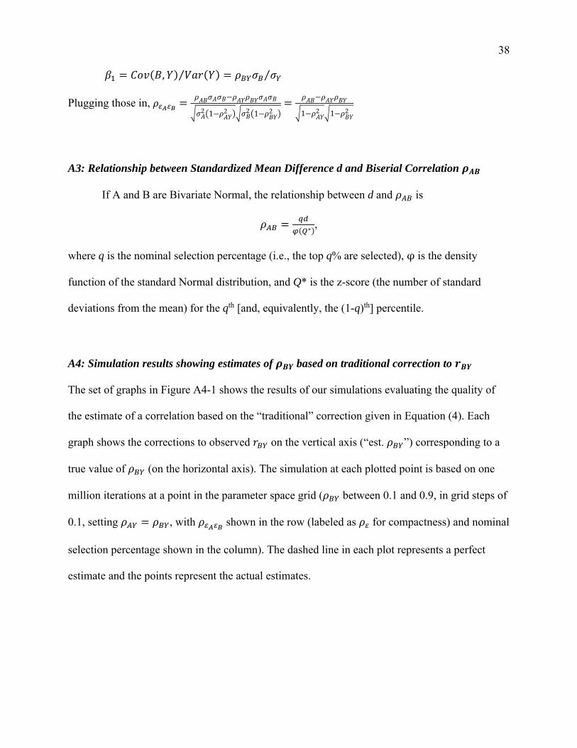
A4: Simulation results showing estimates of based on traditional correction to

The set of graphs in Figure A4-1 shows the results of our simulations evaluating the quality of

the estimate of a correlation based on the “traditional” correction given in Equation (4). Each

graph shows the corrections to observed on the vertical axis (“est. ”) corresponding to a

true value of (on the horizontal axis). The simulation at each plotted point is based on one

million iterations at a point in the parameter space grid ( between 0.1 and 0.9, in grid steps of

0.1, setting , with shown in the row (labeled as for compactness) and nominal

selection percentage shown in the column). The dashed line in each plot represents a perfect

estimate and the points represent the actual estimates.

39

FIGURE A4-1

A5: Non-uniqueness from observed quantities ( , , , )

We present a graphic demonstration that there is not a unique from a set of observed

quantities of ( , , , ). Figure A5-1 shows two iso- surfaces, one for 0.3

and one for 0.9 , for observed values of ( , , ) with a nominal selection

percentage of 10%. (For this counterexample, we set so we can show the surfaces in

three dimensions.) The two surfaces intersect, implying that the same pattern of observed

( , , ) can support different values of . The intersection appears as the ragged line

where the 0.3 surface disappears into the 0.9 surface.

The results are based on one million simulations at each point in the grid of true ( , ,

) space, at intervals of 0.1.

40

FIGURE A5-1

A6: Derivation of Equation (6) in Result 2

We define

≡ ∗ (A6-1)

Using the assumption that and substituting Equation (A6-1) into Equation (3) yields

1 . A6‐2

The marginal contributions of shared error and shared truth to agreement are

1 and 1 . Assuming that the marginal contribution of shared error is

k > 0 times that of shared truth, , we can then solve Equation (A6-2) for as a

function of , resulting in 1 1 .

41

A7: Details of Two-Stage Selection Scenario

The scenario is based on a simulation with the following structure and parameters. In the first

round, 100 candidates are evaluated. Consistent with earlier notation, we denote the correlation

between the latent selection variable and performance as . A subset of the candidates advance

to the second round, where they are evaluated again, and the one deemed best is selected. In the

scenario reported in the text, in the second stage, the correlation between the latent selection

variable and performance is 0.71 (an R2 of 0.5). Finally, the cost of second-stage evaluation is

1% of the standard deviation of Y (performance). A rough estimate of the standard deviation of

Y comes from subtracting the value of a terrible candidate (bottom 5%) from the value of a great

candidate (top 5%) and dividing by 3.29 (two times 1.645, the 95th percentile of a Normal

distribution). All of the initial candidates are evaluated, so the first-round evaluation cost is

fixed, and therefore it does not affect the optimal number of candidates to advance.